Embed Size (px)
Citation preview
Chemical kinetics modelling ofcombustion processes in SI engines
by
Ahmed Faraz KhanB.Sc., M.S.
Submitted in accordance with the requirements for the degree ofDoctor of Philosophy
The University of Leeds
School of Mechanical Engineering
May 2014
The candidate confirms that the work submitted is his own, except where workwhich has formed part of jointly authored publications has been included. Thecontribution of the candidate and the other authors to this work has been ex-plicitly indicated below. The candidate confirms that appropriate credit has beengiven within the thesis where reference has been made to the work of others.
The Figure 2.5 in Chapter 2 has been published in a jointly authored publication:
A.F.Khan and A.A.Burluka. An Investigation of Various Chemical Kinetic Modelsfor the Prediction of Autoignition in HCCI Engine. ASME 2012 Internal CombustionEngine Division Fall Technical Conference, Vancouver, BC, Canada, September 23– 26, 2012. Paper No. ICEF2012-92057, pp. 737-745; doi:10.1115/ICEF2012-92057
The content taken from the above publication for use in this thesis was solelygenerated by the author. The co-author is credited to technical discussion on theresults produced in the publication.
This copy has been supplied on the understanding that it is copyright materialand that no quotation from the thesis may be published without proper acknowl-edgement. The right of Ahmed Faraz Khan to be identified as Author of this workhas been asserted by him in accordance with the Copyright, Designs and PatentsAct 1988.
c© 2014 The University of Leeds and Ahmed Faraz Khan
i
Acknowledgements
The completion of this work owes a lot to the contribution and supportof so many people in my professional and personal life. This is where Ishow my gratitude and acknowledge their support which is certainlyimmeasurable in words.
First and foremost, my supervisor Dr Alexey Burluka, my utmostthanks for the guidance all through the years – you have always beenthere. In addition to all-things-combustion, conversations on worldpolitics were indeed enlightening. I also enjoyed the crash courseon how to appreciate opera while driving down to Northampton –I have seen a couple of them after that with tremendous enjoyment.But above all, many thanks for giving me the opportunity to do thisPhD.
Unfortunately, I did not have much interaction with Prof Chris Shep-pard due to his retirement but his spirit was certainly present in theform of a plethora of SAE papers and titbits from Alex.
My utmost gratitude to a bunch of brilliant engineers and fantastichuman beings at Mahle Powertrain. Without any exaggeration, work-ing with you guys was one of the most enjoyable aspects of my PhD.I have to name some names here: Jens Neumeister, Dave Oudenijew-eme and Paul Freeland, many many thanks for helping me on so manythings. I certainly learned a lot from you guys. Thanks for keeping meon track too, those weekly teleconferences were very useful, not sureabout the Gantt charts though. A special thanks must also go to JohnMitcalf for taking the time out for all the CFD work, thanks to DavidGurney and Andre Bisordi for tips on GT-Power.
I must acknowledge Prof Jeffrey Cash at Imperial College London forthe numerical library MEBDFI, Prof Valeri Golovitchev at ChalmersInstitute of Technology for kindly providing the gasoline mechanism

and Dr Youngchul Ra at University of Wisconsin-Madison for the Re-itz/MultiChem mechanism. Due thanks to Dr Phil Roberts for thepermission to use LUPOE2-D experimental data.
Colleagues in combustion group at Leeds University, who are (in noparticular order) Tawfiq, Navanshu, Ahmed, Dominic, Zhengyang,Nini, Daniel, it was a great pleasure working with you all – my bestwishes for your future. I must pay a special tribute to Dr Graham Con-way who always took the time out to attend to my questions, manythanks for all those discussions on LUSIE and other things in general.Your presence made things a lot easier for me in the early days.
Thanks to the IT staff at the School, in particular, John Hodrien, whosehelp always came with words of wisdom on all-things-LINUX.
My housemates over the years who became my BFFs, Sabina, Lubka,Eva, Danny, Julian, Sandra and Beta, I could not have asked for betterfriends – thank you! BTW I wouldn’t have to do a PhD if I had a pennyfor every time you asked me, “when do you finish?”.
Lastly, because it’s the most important one, my family. I have nowords to thank you with for the limitless love and support you havegiven me over the years. Ami, Abu, Khurram, Ambreen, Babar, Aleezah,thank you all!
Abstract
The need for improving the efficiency and reducing emissions is aconstant challenge in combustion engine design. For spark ignitionengines, these challenges have been targeted in the past decade orso, through ‘engine downsizing’ which refers to a reduction in enginedisplacement accompanied by turbocharging. Besides the benefits ofthis, it is expected to aggravate the already serious issue of engineknock owing to increased cylinder pressure. Engine knock which isa consequence of an abnormal mode of combustion in SI engines, isa performance limiting phenomenon and potentially damaging to theengine parts. It is therefore of great interest to develop capability topredict autoignition which leads to engine knock. Traditionally, ratherrudimentary skeletal chemical kinetics models have been used for au-toignition modelling, however, they either produce incorrect predic-tions or are only limited to certain fuels. In this work, realistic chemi-cal kinetics of gasoline surrogate oxidation has been employed to ad-dress these issues.
A holistic modelling approach has been employed to predict com-bustion, cyclic variability, end gas autoignition and knock propen-sity of a turbocharged SI engine. This was achieved by first devel-oping a Fortran code for chemical kinetics calculations which wasthen coupled with a quasi-dimensional thermodynamic combustionmodelling code called LUSIE and the commercial package, GT-Power.The resulting code allowed fast and appreciably accurate predictionsof the effects of operating condition on autoignition. Modelling wasvalidated through comparisons with engine experimental data at allstages.
Constant volume chemical kinetics modelling of the autoignition ofvarious gasoline surrogate components, i.e. iso-octane, n-heptane,toluene and ethanol, by using three reduced mechanisms revealedhow the conversion rate of relatively less reactive blend components,
toluene and ethanol, is accelerated as they scavenge active radicalformed during the oxidation of n-heptane and iso-octane. Autoigni-tion modelling in engines offered an insight into the fuel-engine inter-actions and that how the composition of a gasoline surrogate shouldbe selected. The simulations also demonstrated the reduced relevanceof research and motor octane numbers to the determination of gaso-line surrogates and that it is crucial for a gasoline surrogate to reflectthe composition of the target gasoline and that optimising its physic-ochemical properties and octane numbers to match those of the gaso-line does not guarantee that the surrogate will mimic the autoignitionbehaviour of gasoline.
During combustion modelling, possible deficiencies in in-cylinder tur-bulence predictions and possible inaccuracies in turbulent entrain-ment velocity model required an optimisation of the turbulent lengthscale in the eddy burn-up model to achieve the correct combustionrate. After the prediction of a correct mean cycle at a certain enginespeed, effects of variation in intake air temperature and spark timingwere studied without the need for any model adjustment. Autoigni-tion predictions at various conditions of a downsized, turbochargedengine agreed remarkably well with experimental values. When cou-pled with a simple cyclic variability model, the autoignition predic-tions for the full spectrum of cylinder pressures allowed determina-tion of a percentage of the severely autoigniting cycles at any givenspark timing or intake temperature. Based on that, a knock-limitedspark advance was predicted within an accuracy of 2◦ of crank angle.
Contents
Contents v
List of Figures ix
List of Tables xvii
Nomenclature xix
1 Introduction to topic and terminologies 11.1 Introduction and motivation . . . . . . . . . . . . . . . . . . . . . . . 11.2 Scope of this work . . . . . . . . . . . . . . . . . . . . . . . . . . . . . 31.3 Thesis organisation . . . . . . . . . . . . . . . . . . . . . . . . . . . . 41.4 Autoignition and knock . . . . . . . . . . . . . . . . . . . . . . . . . 5
1.4.1 Factors affecting engine knock . . . . . . . . . . . . . . . . . 61.4.1.1 Engine design and operating conditions . . . . . . 61.4.1.2 Fuel effects . . . . . . . . . . . . . . . . . . . . . . . 8
1.5 Ignition delay time measurements . . . . . . . . . . . . . . . . . . . 101.6 Autoignition modelling . . . . . . . . . . . . . . . . . . . . . . . . . 12
2 Principles and modelling of chemical kinetics 152.1 Introduction . . . . . . . . . . . . . . . . . . . . . . . . . . . . . . . . 152.2 Chemical kinetics fundamentals . . . . . . . . . . . . . . . . . . . . . 16
2.2.1 Rate of formation or depletion of species . . . . . . . . . . . 182.2.1.1 Three-body collision reactions . . . . . . . . . . . . 19
2.2.2 Pressure dependant or fall-off reactions . . . . . . . . . . . . 202.2.3 Thermodynamic properties . . . . . . . . . . . . . . . . . . . 22
2.3 Numerical integration . . . . . . . . . . . . . . . . . . . . . . . . . . 232.4 Code development . . . . . . . . . . . . . . . . . . . . . . . . . . . . 232.5 Chemical kinetics mechanisms . . . . . . . . . . . . . . . . . . . . . 25
v
CONTENTS
2.5.1 Andrae model . . . . . . . . . . . . . . . . . . . . . . . . . . . 282.5.2 Golovitchev model . . . . . . . . . . . . . . . . . . . . . . . . 292.5.3 Reitz model . . . . . . . . . . . . . . . . . . . . . . . . . . . . 30
2.6 Code validation . . . . . . . . . . . . . . . . . . . . . . . . . . . . . . 302.7 Autoignition simulation results . . . . . . . . . . . . . . . . . . . . . 332.8 Practical gasoline surrogates . . . . . . . . . . . . . . . . . . . . . . . 362.9 Gasoline surrogate formulation . . . . . . . . . . . . . . . . . . . . . 422.10 Summary . . . . . . . . . . . . . . . . . . . . . . . . . . . . . . . . . . 44
3 Hydrocarbon oxidation chemistry 463.1 Introduction . . . . . . . . . . . . . . . . . . . . . . . . . . . . . . . . 463.2 General features of hydrocarbon oxidation . . . . . . . . . . . . . . 49
3.2.1 Low temperature oxidation . . . . . . . . . . . . . . . . . . . 493.2.2 High temperature oxidation . . . . . . . . . . . . . . . . . . . 53
3.3 Numerical predictions of oxidation pathways . . . . . . . . . . . . . 543.3.1 Iso-octane . . . . . . . . . . . . . . . . . . . . . . . . . . . . . 543.3.2 N-heptane . . . . . . . . . . . . . . . . . . . . . . . . . . . . . 573.3.3 Toluene . . . . . . . . . . . . . . . . . . . . . . . . . . . . . . 60
3.3.3.1 Effect of doping on toluene oxidation . . . . . . . . 643.3.3.2 Effects of binary blending on toluene ignition de-
lay time . . . . . . . . . . . . . . . . . . . . . . . . . 663.3.4 Ethanol . . . . . . . . . . . . . . . . . . . . . . . . . . . . . . . 673.3.5 Effect of toluene on PRF oxidation . . . . . . . . . . . . . . . 693.3.6 Effect of ethanol on PRF oxidation . . . . . . . . . . . . . . . 763.3.7 Discussion of chemical kinetics modelling . . . . . . . . . . 77
4 Description of SI engine combustion processes 814.1 Introduction . . . . . . . . . . . . . . . . . . . . . . . . . . . . . . . . 814.2 Turbulence . . . . . . . . . . . . . . . . . . . . . . . . . . . . . . . . . 81
4.2.1 Statistical quantification of turbulence . . . . . . . . . . . . . 824.2.1.1 Turbulent velocity and turbulence intensity . . . . 824.2.1.2 Turbulent length scales . . . . . . . . . . . . . . . . 83
4.3 Background to combustion and flames . . . . . . . . . . . . . . . . . 864.3.1 Laminar premixed flames . . . . . . . . . . . . . . . . . . . . 87
4.3.1.1 Instabilities in laminar premixed flames . . . . . . 894.3.2 Turbulent premixed flames . . . . . . . . . . . . . . . . . . . 90
4.3.2.1 Regimes of premixed combustion . . . . . . . . . . 91
vi
CONTENTS
4.4 Modelling of combustion in SI engines . . . . . . . . . . . . . . . . . 934.5 Zero/multi-zone thermodynamic modelling . . . . . . . . . . . . . 94
4.5.1 Zero dimensional thermodynamic modelling . . . . . . . . . 944.5.2 Two-zone thermodynamic modelling . . . . . . . . . . . . . 944.5.3 Three-zone thermodynamic modelling . . . . . . . . . . . . 954.5.4 Turbulent burning velocity . . . . . . . . . . . . . . . . . . . 96
4.6 Introduction to LUSIE . . . . . . . . . . . . . . . . . . . . . . . . . . 1014.6.1 Motoring simulation . . . . . . . . . . . . . . . . . . . . . . . 1014.6.2 Heat transfer . . . . . . . . . . . . . . . . . . . . . . . . . . . 1014.6.3 Blowby . . . . . . . . . . . . . . . . . . . . . . . . . . . . . . . 1024.6.4 Laminar burning velocity . . . . . . . . . . . . . . . . . . . . 1024.6.5 Autoignition modelling . . . . . . . . . . . . . . . . . . . . . 103
4.6.5.1 Species translation between LUSIE/GT-LU and chem-ical kinetics mechanisms . . . . . . . . . . . . . . . 104
4.6.5.2 Autoignition criteria . . . . . . . . . . . . . . . . . . 1054.6.6 Cyclic variability . . . . . . . . . . . . . . . . . . . . . . . . . 106
4.7 Introduction to GT-Power . . . . . . . . . . . . . . . . . . . . . . . . 1074.7.1 In-cylinder flow models . . . . . . . . . . . . . . . . . . . . . 108
4.7.1.1 Swirl, radial and axial velocities . . . . . . . . . . . 1104.7.1.2 Turbulence model . . . . . . . . . . . . . . . . . . . 111
4.8 Introduction to GT-LU . . . . . . . . . . . . . . . . . . . . . . . . . . 1124.9 CFD modelling of turbulence . . . . . . . . . . . . . . . . . . . . . . 1134.10 Description of the test cases . . . . . . . . . . . . . . . . . . . . . . . 115
4.10.1 LUPOE2-D . . . . . . . . . . . . . . . . . . . . . . . . . . . . . 1154.10.2 Mahle Di3 engine . . . . . . . . . . . . . . . . . . . . . . . . . 119
5 Autoignition in LUPOE2-D 1225.1 Introduction . . . . . . . . . . . . . . . . . . . . . . . . . . . . . . . . 1225.2 Supporting experiments . . . . . . . . . . . . . . . . . . . . . . . . . 123
5.2.1 Normal burning rates and cyclic variability . . . . . . . . . . 1235.2.2 Fuel effects on knock onset and its statistical variation . . . 124
5.3 LUPOE2-D modelling . . . . . . . . . . . . . . . . . . . . . . . . . . 1265.4 Results and discussion . . . . . . . . . . . . . . . . . . . . . . . . . . 127
6 Combustion and autoignition modelling in a turbocharged SI engine 1336.1 Introduction . . . . . . . . . . . . . . . . . . . . . . . . . . . . . . . . 1336.2 Di3 engine operating conditions . . . . . . . . . . . . . . . . . . . . 135
vii
CONTENTS
6.3 GT-Power model validation . . . . . . . . . . . . . . . . . . . . . . . 1366.4 In-cylinder turbulence . . . . . . . . . . . . . . . . . . . . . . . . . . 1376.5 Combustion modelling results . . . . . . . . . . . . . . . . . . . . . . 139
6.5.1 Spark timing and charge temperature sweeps . . . . . . . . 1486.6 Cyclic variability modelling results . . . . . . . . . . . . . . . . . . . 1486.7 Autoignition modelling results . . . . . . . . . . . . . . . . . . . . . 154
6.7.1 Gasoline surrogates . . . . . . . . . . . . . . . . . . . . . . . 1556.7.2 Knock in Di3 engine . . . . . . . . . . . . . . . . . . . . . . . 1566.7.3 Autoignition modelling for the mean cycles . . . . . . . . . . 1606.7.4 Cyclic variability and autoignition . . . . . . . . . . . . . . . 164
6.8 Fuel-engine interaction . . . . . . . . . . . . . . . . . . . . . . . . . . 1696.9 General discussion and conclusions . . . . . . . . . . . . . . . . . . 170
7 Conclusions and future recommendations 1747.1 Introduction . . . . . . . . . . . . . . . . . . . . . . . . . . . . . . . . 1747.2 Conclusions . . . . . . . . . . . . . . . . . . . . . . . . . . . . . . . . 1757.3 Future recommendations . . . . . . . . . . . . . . . . . . . . . . . . . 177
Appendix A 179A.1 User guide (GT-LU v7.3) . . . . . . . . . . . . . . . . . . . . . . . . . 179
A.1.1 Migrating from a non-predictive GT-Power model to a pre-dictive GT-LU model . . . . . . . . . . . . . . . . . . . . . . . 179A.1.1.1 Burn rate . . . . . . . . . . . . . . . . . . . . . . . . 180A.1.1.2 UserModel for turbulent flame speed . . . . . . . . 181A.1.1.3 UserModel for autoignition . . . . . . . . . . . . . 181A.1.1.4 Flow object (EngCylFlow) . . . . . . . . . . . . . . 181
A.1.2 External turbulence file format . . . . . . . . . . . . . . . . . 183A.1.3 Chemical kinetic mechanisms . . . . . . . . . . . . . . . . . . 183A.1.4 Cyclic variability in GT-LU . . . . . . . . . . . . . . . . . . . 184
A.1.4.1 Setting cyclic variability in a GT-LU model . . . . . 184A.1.4.2 Convergence control and number of cycle to be ran 185
A.1.5 GT-LU outputs . . . . . . . . . . . . . . . . . . . . . . . . . . 185
References 186
viii
List of Figures
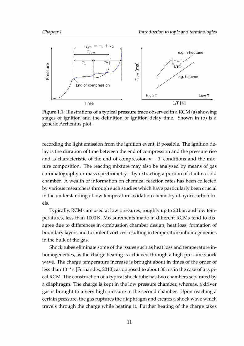
1.1 Illustrations of a typical pressure trace observed in a RCM (a) show-ing stages of ignition and the definition of ignition delay time.Shown in (b) is a generic Arrhenius plot. . . . . . . . . . . . . . . . . 11
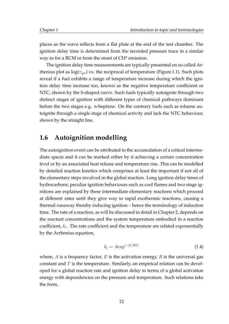
1.2 Autoignition prediction using the D&E model and Livengood-Wuintegral for the in-cylinder pressure of the Di3 engine (see Sec-tion 4.10.2) recorded at 2000 rpm. . . . . . . . . . . . . . . . . . . . . 14
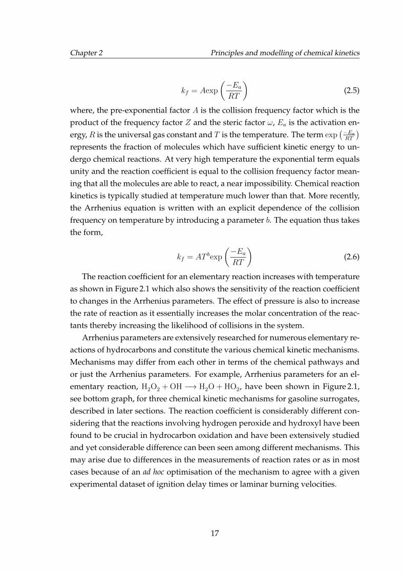
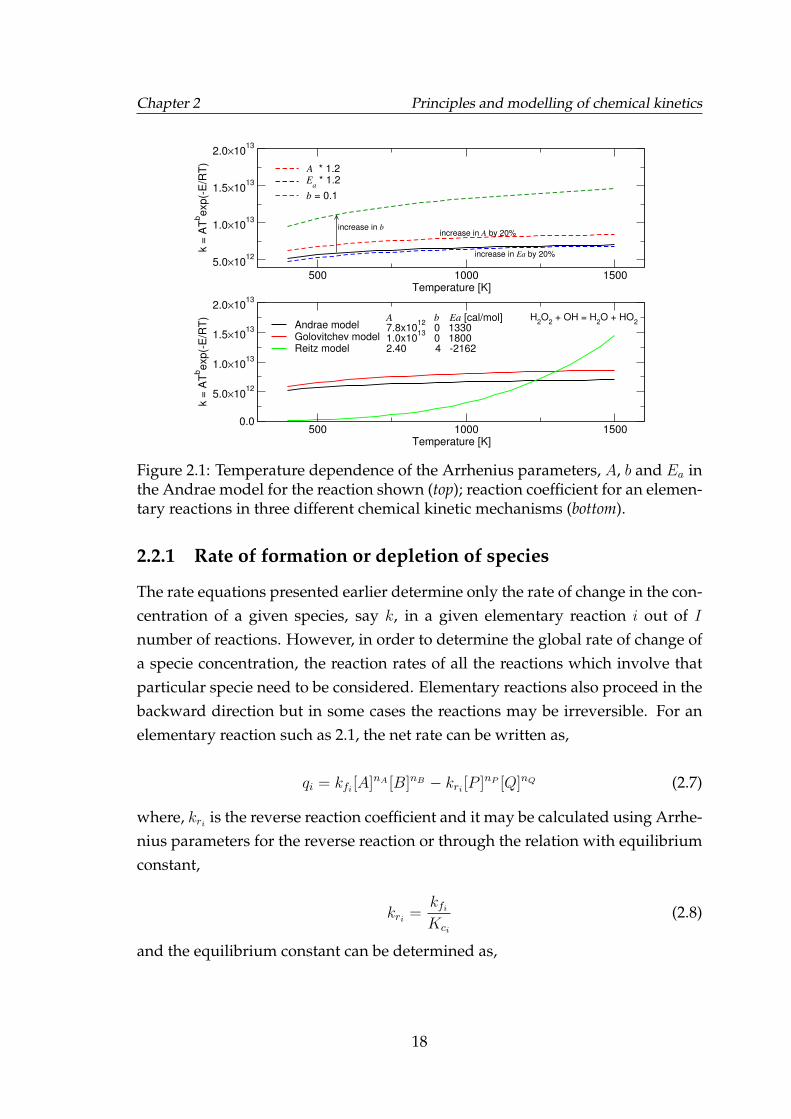
2.1 Temperature dependence of the Arrhenius parameters, A, b and Eain the Andrae model for the reaction shown (top); reaction coeffi-cient for an elementary reactions in three different chemical kineticmechanisms (bottom). . . . . . . . . . . . . . . . . . . . . . . . . . . . 18
2.2 Block diagram showing various routines which comprise the chem-ical kinetics solver. The routines developed in this work are kin-reader.f and KineticModule.f. . . . . . . . . . . . . . . . . . . . . . . 24
2.3 Block diagram showing parts of the chemical kinetics code wherevarious calculations are done. . . . . . . . . . . . . . . . . . . . . . . 24
2.4 Plot showing relative sizes of various mechanisms from the litera-ture in terms of their number of species and elementary reactions,some of these mechanisms have been studied in this work. . . . . . 25
2.5 Ignition delay time predictions of 9 different mechanisms of dif-ferent orders of complexity. Simulations for detailed and semi-detailed mechanisms were done in Cosilab, whereas, reduced andskeletal models were implemented in Fortran. . . . . . . . . . . . . 27
2.6 Comparison of ignition delay predictions made by the Leeds Chem-istry Solver and Chemkin II for n-heptane and iso-octane using theReitz model. . . . . . . . . . . . . . . . . . . . . . . . . . . . . . . . . 31
ix
LIST OF FIGURES
2.7 Comparison of ignition delay predictions made by the Leeds Chem-istry Solver, Cosilab and Chemkin II for iso-octane using the An-drae model. . . . . . . . . . . . . . . . . . . . . . . . . . . . . . . . . 31
2.8 Comparison of ignition delay predictions made by the Leeds Chem-istry Solver and Chemkin II for toluene using the Golovitchev model. 32
2.9 Effect of the integration time step on ignition delay time and com-putational time. . . . . . . . . . . . . . . . . . . . . . . . . . . . . . . 32
2.10 Low pressure ignition delay time predictions (lines) made by thethree reduced chemical kinetic mechanisms for four key gasolinesurrogate components. Symbols represent shock tube measure-ments; (a) [Fieweger et al., 1997] (b) [Silke et al., 2005] (c) [Shenet al., 2009] (d) [Cancino et al., 2010]. . . . . . . . . . . . . . . . . . . 34
2.11 High pressure ignition delay times predictions (lines) made by thethree reduced chemical kinetic mechanisms for four key gasolinesurrogate components. Symbols represent shock tube measure-ments; (a) [Fieweger et al., 1997] (b) [Fieweger et al., 1997; Hart-mann et al., 2011] (c) [Davidson et al., 2005] (d) [Cancino et al., 2011]. 35
2.12 Comparisons of ignition delay time measurements by Fiewegeret al. [1997] and predictions by using the Andrae model (a), Golovitchevmodel (b) and Reitz model (c). . . . . . . . . . . . . . . . . . . . . . . 37
2.13 Comparison of predicted Ignition delay times of the Gauthier-ATRF and a gasoline surrogate by Fikri et al. [2008] to the shock tubeand RCM measurements. . . . . . . . . . . . . . . . . . . . . . . . . 40
2.14 Comparison of predicted ignition delay times of the stoichiometricair mixture of surrogate comprising iso-octane 37.8%/n-heptane10.2%/toluene 12%/ethanol 40% by volume, with its measurementsby Cancino et al. [2009] at initial pressures of 10 bar (a), 30 bar (b)and 50 bar (c). . . . . . . . . . . . . . . . . . . . . . . . . . . . . . . . 41
3.1 A generic illustration of the low, intermediate and high tempera-ture pathway regimes for alkanes. Adapted from [Miller et al., 2005]. 48
3.2 Predicted carbon fraction of the key intermediate species produced.See Table 3.1 for grouped species. . . . . . . . . . . . . . . . . . . . . 56
3.3 Predicted carbon fraction of the key intermediate species produced. 563.4 Predicted carbon fraction of the key intermediate species produced. 57
x
LIST OF FIGURES
3.5 Carbon fraction of carbon containing key intermediates (left axis).Molar concentration of OH, hydrogen peroxide and water (rightaxis). . . . . . . . . . . . . . . . . . . . . . . . . . . . . . . . . . . . . 58
3.6 Carbon fraction of carbon containing key intermediates. . . . . . . 593.7 Carbon fraction of carbon containing key intermediates. . . . . . . 593.8 Molar concentration of the key intermediates formed during the
pre-ignition reactions of toluene as predicted by the Andrae model. 623.9 Molar concentration of the key intermediates formed during the
pre-ignition reactions of toluene as predicted by the GolovitchevModel. . . . . . . . . . . . . . . . . . . . . . . . . . . . . . . . . . . . 63
3.10 Molar concentration of the key intermediates formed during thepre-ignition reactions of toluene as predicted by the Reitz Model. . 63
3.11 Effect of hydrogen peroxide doping on induction time of tolueneas predicted by the Andrae model. . . . . . . . . . . . . . . . . . . . 65
3.12 Ignition delay times of binary blends of toluene with benzene, iso-octane and n-heptane for stoichiometric mixtures with air. . . . . . 66
3.13 Molar concentration of the key intermediates formed during thepre-ignition reactions of ethanol as predicted by the Andrae model. 68
3.14 Molar concentration of the key intermediates formed during thepre-ignition reactions of ethanol as predicted by the Reitz Model. . 69
3.15 Ignition delay times of various blends of PRF90 and toluene. . . . . 703.16 Temperature profiles of neat iso-octane, n-heptane, PRF90, PRF90
+ 25% toluene and 50% toluene by moles as predicted by Andraemodel (a), Golovitchev model (b) and Reitz model (c). . . . . . . . . 71
3.17 Variation in the concentration profiles of the key species and activecentres of PRF90 due to the presence of an increasing molar contentof toluene as predicted by the Andrae model. . . . . . . . . . . . . . 72
3.18 Carbon fractions of iso-octane and intermediates specific to it forfour fuels; pure iso-octane (black lines), PRF90 (red lines) and PRF90+ 25% by mole toluene (blue lines) and PRF90 + 25% by moleethanol (green lines). . . . . . . . . . . . . . . . . . . . . . . . . . . . 74
3.19 Predicted benzaldehyde carbon fraction of toluene (a) and acetalde-hyde carbon fraction of ethanol (b) when in pure form and whenblended with PRF90 by 25% by moles. . . . . . . . . . . . . . . . . . 75
xi
LIST OF FIGURES
3.20 Carbon fractions of n-heptane and its ketohydroperoxide as pre-dicted for four fuels; pure n-heptane (black lines), PRF90 (red lines)and PRF90 + 25% by mole toluene (blue lines) and PRF90 + 25% bymole ethanol (green lines). . . . . . . . . . . . . . . . . . . . . . . . . 75
3.21 Temperature profiles of iso-octane, n-heptane, PRF90 and its blendswith ethanol by molar percentages of 5%, 25% and 50% as pre-dicted by the Andrae model (a), Golovitchev model (b) and theReitz model (c) at 40 bar and 700 K. . . . . . . . . . . . . . . . . . . . 78
3.22 Experimentally measured ignition delay times from the literaturefor neat iso-octane, toluene and ethanol with air (φ=1) at similarpressures. . . . . . . . . . . . . . . . . . . . . . . . . . . . . . . . . . . 79
4.1 (a) An illustration of velocity fluctuations at a fixed point in a steadyturbulent flow-field. (b) A typical autocorrelation function and thedefinition of the integral (L) and Taylor (λ) length scales. . . . . . . 83
4.2 Schematic showing temperature and concentration profiles associ-ated with a 1−D premixed adiabatic flame; adapted from Griffithsand Barnard [1995]. . . . . . . . . . . . . . . . . . . . . . . . . . . . . 88
4.3 Schematic showing a 1−D planar flame and its associated burningspeeds. . . . . . . . . . . . . . . . . . . . . . . . . . . . . . . . . . . . 89
4.4 Schematics showing (a) the Darrieus-Landau hydrodynamic insta-bility and (b) thermo-diffusive effects in a wrinkled laminar pre-mixed flame. . . . . . . . . . . . . . . . . . . . . . . . . . . . . . . . . 90
4.5 Borghi diagram . . . . . . . . . . . . . . . . . . . . . . . . . . . . . . 924.6 Typical behaviour of various Zimont-Lipatnikov model quantities.
Calculations made for Di3 engine, see Section 4.10.2 for engine de-tails, at 2000 rpm, 20 bar bmep. The ul is determined for a stoichio-metric mixture of indolene and air. . . . . . . . . . . . . . . . . . . . 99
4.7 Flow of data and sequence of operations carried out in autoignitionmodelling. AI stands for autoignition. . . . . . . . . . . . . . . . . . 104
4.8 Graphical schematic of the LUPOE2-D GT-Power model employedin this work for GT-LU modelling studies of combustion, cyclicvariability and autoignition. . . . . . . . . . . . . . . . . . . . . . . . 109
4.9 Illustration showing the combustion chamber divided in four re-gions for each of which a pair of turbulent kinetic energy and dis-sipation rate equations are solved. . . . . . . . . . . . . . . . . . . . 110
4.10 Flow of data and sequence of operations carried out by GT-LU . . . 114
xii
LIST OF FIGURES
4.11 An annotated cross-section view of LUPOE2-D [Abdi Aghdam,2003]. . . . . . . . . . . . . . . . . . . . . . . . . . . . . . . . . . . . . 117
4.12 An annotated CAD drawing of LUPOE2-D and its auxiliaries. Alsoshown is the top and side optical access and laser positioning forLDV and PIV experiments [Ling, 2011]. . . . . . . . . . . . . . . . . 118
4.13 A CAD generated view of the Mahle Di3 engine. . . . . . . . . . . . 1204.14 Views of the cylinder head (left) and the piston crown (right) of the
Mahle Di3 engine. . . . . . . . . . . . . . . . . . . . . . . . . . . . . . 121
5.1 A set of 100 fired cycles for ULG90 shown by grey lines. Black lineshows the ensemble average of smoothed firing cycles. . . . . . . . 124
5.2 Statistical variation of experimental knock onsets for the four testedfuels. Squares: mean knock onset, diamonds: earlier and latestknock onsets, box: 25/75 percentile, whiskers: 5/95 percentile. . . . 125
5.3 Knocking experimental cycles of the four fuels with similar pres-sures to that of the pre-knock pressure of the mean ULG90 cycle. . 126
5.4 Comparison of the predicted and experimental autoignition onsetsfor PRF90, TRF90 and iso-octane. . . . . . . . . . . . . . . . . . . . . 127
5.5 The τign contour map of PRF90 as predicted by the Andrae modelsuperimposed with the unburned zone p−T history of LUPOE2-Dand typical RON/MON tests. . . . . . . . . . . . . . . . . . . . . . . 128
5.6 The τign contour map of TRF90 as predicted by the Andrae modelsuperimposed by the unburned zone p − T history of LUPOE2-Dand typical RON/MON tests. . . . . . . . . . . . . . . . . . . . . . . 129
5.7 Unburned zone p−T history of LUPOE2-D and typical RON/MONtests superimposed on the τign contour map of iso-octane as pre-dicted by the Andrae Model. . . . . . . . . . . . . . . . . . . . . . . 129
6.1 Peak bmep curve of the Di3 engine, showing the operating pointsstudied in this Chapter. . . . . . . . . . . . . . . . . . . . . . . . . . . 135
6.2 log-log charts showing the in-cylinder pressure and volume at theconditions studied. Black dashed line represents the engine testmeasurements. Solid red lines represent simulation results usingnon-predictive combustion model. . . . . . . . . . . . . . . . . . . . 137
6.3 CFD modelling results showing u′ and L for the five operating con-ditions. c & d show the close up for crank angles around TDCF. . . 138
xiii
LIST OF FIGURES
6.4 Comparison of u′ and L obtained by CFD modelling and the GT-Power’s k − ε model during the time of flame propagation. Blacklines: k − ε model in GT-Power; red lines: CFD modelling. . . . . . 139
6.5 Effect of Taylor microscale variation in the eddy burn-up model,on cylinder pressure. Grey lines show simulated cyclic variation. . 140
6.6 Comparison of the simulated mean cycles, using as an input, theturbulence from CFD modelling (blue lines) and the k− ε model inGT-Power (red lines). Black dashed lines represent engine test data. 142
6.7 Effect of variation in engine speed and load (boost pressure) on (a)kinematic viscosity, ν, (b) unburned charge density, ρ, (c) Reynoldsnumber, Re, and (d) Thermal diffusivity. . . . . . . . . . . . . . . . . 143
6.8 Effect of variation in engine speed and load (boost pressure) onvarious turbulent length scales and the laminar flame thickness. . . 144
6.9 Effect of load (boost pressure) and speed variation on the flameregime on a Borghi diagram. See Table 6.1 and Figure 6.1 for detailson the operating points. . . . . . . . . . . . . . . . . . . . . . . . . . 145
6.10 10%, 50% and 90% fuel mass fraction burned (MFB) points forspark timing and inlet charge temperature sweeps for Di3 engineoperating conditions: (a) I, (b) II, (c) III, (d) IV as in Table 6.1. Sim-ulations are represented by lines. Spark timing for charge temper-ature sweeps have also been shown. . . . . . . . . . . . . . . . . . . 149
6.11 144 perturbed cycles of rms velocity according to a Gaussian dis-tribution. The black line represents the mean rms velocity. . . . . . 150
6.12 Quantile-quantile plots comparing the generated (expected) Gaus-sian multipliers for (top) φ and (bottom) u′, to a reference Gaussiandistribution. . . . . . . . . . . . . . . . . . . . . . . . . . . . . . . . . 151
6.13 Comparison of simulated and actual peak cylinder pressure at cor-responding crank angle. The mean peak pressure, Pmax, and pres-sures at ±2σ have also been indicated. . . . . . . . . . . . . . . . . . 152
6.14 Comparison of simulated and actual peak cylinder pressure at cor-responding crank angle. The mean peak pressure, Pmax, and pres-sures at ±2σ have also been indicated. . . . . . . . . . . . . . . . . . 153
6.15 Comparison of simulated and actual Pmax frequency. Correspond-ing normal distribution curves scaled to the maximum have alsobeen shown. . . . . . . . . . . . . . . . . . . . . . . . . . . . . . . . . 154
xiv
LIST OF FIGURES
6.16 Comparison of simulated and actual θPmax frequency. Correspond-ing normal distribution curves scaled to the maximum have alsobeen shown. . . . . . . . . . . . . . . . . . . . . . . . . . . . . . . . . 155
6.17 Examples of a normal (non-knocking) cycle and a knocking cycle atlow engine speed with corresponding filtered pressure oscillationsindicating the knock onset. . . . . . . . . . . . . . . . . . . . . . . . . 158
6.18 Examples of a normal (non-knocking) cycle and a knocking cycleat high engine speed with corresponding filtered pressure oscilla-tions indicating the knock onset in dashed red lines. . . . . . . . . . 158
6.19 Maximum amplitude of pressure oscillations vs. correspondingknock onset for the six charge temperatures at 5000 rpm, shown assymbols. Red lines: linear best fit; green lines: average knock onset. 159
6.20 Top: simulated burned gas residuals as percentage by mass of thetotal charge at cycle start; bottom: molar concentration of burnedresidual species. . . . . . . . . . . . . . . . . . . . . . . . . . . . . . . 160
6.21 Selected middle cycles which are within 1.5% of the mean cycleupto 15◦ aTDC. Mean knock onsets for all cycles and selected meancycles have also been shown. . . . . . . . . . . . . . . . . . . . . . . 161
6.22 Comparison of predicted autoignition onsets to mean knock onsetsfor all the cycles and those of the selected middle cycles. . . . . . . 162
6.23 Autoignition onsets predicted for various fuels of different compo-sitions at the same unburned p−T conditions using three chemicalmechanisms. . . . . . . . . . . . . . . . . . . . . . . . . . . . . . . . . 163
6.24 Comparison of predicted autoignition onsets to mean knock onsetsfor all the cycles and those of the selected middle cycles. . . . . . . 164
6.25 Variation in Knock Index, KI, for typical range of values of Tunb.,mb and engine speed. . . . . . . . . . . . . . . . . . . . . . . . . . . . 166
6.26 Effect of charge heating and spark advance on knock intensity,∆Pai/P , at different speed and load conditions of the Di3 enginetests. . . . . . . . . . . . . . . . . . . . . . . . . . . . . . . . . . . . . 167
6.27 Plots showing Pai/P vs. corresponding predicted autoignition on-set for full range cycles at various spark timings. . . . . . . . . . . . 168
6.28 Comparison of computed knock frequencies based on various knockindices to the experimental knock frequency shown as symbols. . . 169
xv
LIST OF FIGURES
6.29 The τign contour map of the RON 95 properties based surrogate ofcomposition, iso-octane 28.42%/n-heptane 16.33%/toluene 33.07%/ethanol5.35%/iso-butene 16.84% by volume, computed using the Andraemodel. The cylinder pressure and unburned zone temperature his-tories of Di3 engine have been superimposed. . . . . . . . . . . . . . 171
6.30 Autoignition onsets predicted using the properties based surro-gate with Andrae model and the skeletal Keck model at Di3 enginespeeds of 2000, 3500 and 5000 rpm. . . . . . . . . . . . . . . . . . . . 172
1 Details of the GT-Power user templates which have been used toincorporate various LUSIE submodels. . . . . . . . . . . . . . . . . . 180
2 Inputs to the UserModel for turbulent flame speed model. . . . . . 1813 Inputs to the UserModel for autoignition subroutines. . . . . . . . . 1824 Inputs to the UserModel induce fluctuations in air to fuel ratio or
equivalence ratio. . . . . . . . . . . . . . . . . . . . . . . . . . . . . . 185
xvi
List of Tables
2.1 Volumetric composition of various gasoline surrogate blends foundin the literature for which extensive shock tube and RCM measure-ments have been made. . . . . . . . . . . . . . . . . . . . . . . . . . . 38
3.1 Key intermediate species for iso-octane oxidation identified in thethree reduced mechanisms during the low/intermediate tempera-ture regimes. . . . . . . . . . . . . . . . . . . . . . . . . . . . . . . . . 54
4.1 Design specifications of the LUPOE2-D as used in experiments byRoberts [2010]. . . . . . . . . . . . . . . . . . . . . . . . . . . . . . . . 116
4.2 Main cylinder and cranktrain design specifications of the MahleDi3 turbocharged downsized engine. . . . . . . . . . . . . . . . . . . 120
5.1 LUPOE2-D operating conditions at which ULG90, PRF90, TRF90and iso-octane were tested. . . . . . . . . . . . . . . . . . . . . . . . 123
5.2 Key properties and volumetric composition of ULG90 and its sur-rogates. Predicted surrogate autoignition onsets for the ULG90p− T condition of Fig. 5.3 have also been tabulated. . . . . . . . . . 131
6.1 Five Di3 operating conditions studied in this work. These con-ditions are referred here onwards to by the corresponding romannumeral. . . . . . . . . . . . . . . . . . . . . . . . . . . . . . . . . . . 136
6.2 Specifications of the two fuels used in Di3 engine tests. . . . . . . . 1366.3 Taylor microscale multiplier, Cλ, used in this work to predict the
mean cycles of the four engine load-speed points. . . . . . . . . . . 1416.4 Key properties and volumetric composition of E5-95/85 fuel and
its surrogates. A, G, and R indicate the Andrae, Golovitchev andReitz models. . . . . . . . . . . . . . . . . . . . . . . . . . . . . . . . 156
xvii

LIST OF TABLES
6.5 Key properties and volumetric composition of 102RON fuel andits surrogate. The surrogate is a composition based surrogate con-taining high octane components; diisobutylene and ethanol whichreplaces MTBE. . . . . . . . . . . . . . . . . . . . . . . . . . . . . . . 157
xviii
Nomenclature
Roman and Greek Symbols
Symbol Units DescriptionA m2, AreaCz – Zimont burning velocity model constanta m/sec Speed of sound in a gasα 1/sec Stretch rateB m Engine boreCλ - Taylor microscale multiplierδl m Laminar flame thicknessD m2/sec Mass diffusivityDa – Damkholer numberKa – Karlovitz numberk m 2/s2 Turbulent kinetic energyκ m 2/s Thermal diffusivityLe – Lewis numberL m Turbulent integral length scaleλ m Turbulent Taylor microscaleη m Turbulent Kolmogorov length scalep Pa Pressureφ – Equivalence Ratiom kg Massm kg/sec Mass flow rateρ kg / m3 Densityr m RadiusRe - Reynolds NumberT K Temperaturet sec Timeτign ms Ignition delay time
xix
NOMENCLATURE
u m/sec Burning Velocityu′ m/sec Rms turbulent velocity
Abbreviations
aTDC After top dead centrebTDC Before top dead centreoCA Degrees of crank angle rotationCR Compression ratioDNS Direct numerical simulationECU Electronic control unitEGR Exhaust gas recirculationEPC/EVC Exhaust port closure / exhaust valve closureHCCI Homogeneous charge compression ignitionIMEP Indicated mean effective pressureIPC/IVC Intake port closure / intake valve closureK Kalghatgi octane index correction factorLDV Laser doppler velocimetryLES Large eddy simulationLUPOE1/2-D Leeds university ported optical engine (Mk I/II) disc
configurationLUSIE Leeds university spark ignition engine (simulation soft-
ware)LUSIEDA Leeds university spark ignition engine data analysisMATLAB Matrix LaboratoryMBT Maximum Brake TorqueMON Motor octane numberNTC Negative temperature coefficientOI Octane indexON Octane NumberPIV Particle image velocimetryPRF Primary reference fuelrms Root mean squarerpm Revolutions per minuteRON Research octane numberS Fuel sensitivity
xx
NOMENCLATURE
SI Spark ignitionTDC Top dead centreTDCF Firing, top dead centreTKE Turbulent kinetic energyVVT Variable valve timingVVL Variable vale liftWOT Wide open throttle
Subscripts
b Burnedi Intakel Laminart Turbulentr Reaction (burnt)u Unburned
xxi
Chapter 1
Introduction to topic andterminologies
1.1 Introduction and motivation
Combustion engines had a tremendous impact on society at the time of their firstuse and to this day are one of the most important energy conversion devices andsee wide usage in transport sector and electric power generation. Internal com-bustion engines, or ICEs, have come a long way since their inception and modernday spark ignition (SI) engines are able to reach thermal efficiency around 35%and compression ignition (CI) engines reaching slightly higher figures. The mostimportant factors in the development of new engine technologies are the emis-sion legislation, fuel efficiency and viability of renewable fuels for engine use.
Taylor [2008] in his ICE technology review predicted an improvement in fuelefficiency of about 6 to 15 ±2% for gasoline and compressed natural gas enginesusing port fuel injection and direct injection; and an improvement of 7% for CIengines reaching efficiency levels of 52%, owing to pressure charging, reducedfrictional losses and improved combustion control. SI engine development in thepast decade or so has already incorporated ideas such as direct injection, heavyturbocharging and ’downsizing’ which is brought about by a reduction in enginedisplacement. This is achieved by either cylinder deactivation which is popularin USA or reduction in number of cylinders and/or reduction in cylinder ca-pacity, an approach taken by both American and European car makers. Engine
Chapter 1 Introduction to topic and terminologies
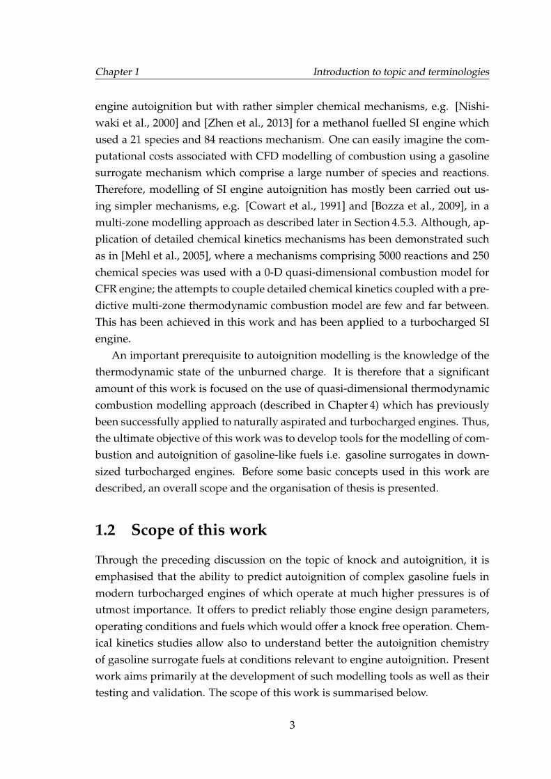
downsizing thus exploits the advantages of reduced frictional losses, no pumpinglosses due to turbocharging which improves part-load performance while main-taining peak performance. Some examples of downsizing report considerableimprovements of drive cycle fuel consumption in comparison to the baseline en-gine while maintaining similar level of performance, e.g. 25-30% fuel consump-tion improvement for a 50% downsized engine [Lumsden et al., 2009], 20% for a60% downsized engine [Attard et al., 2010] and 17% for a 40% downsized engine[Han et al., 2007]. Fuel efficiency advantages also reflect in lower CO2 emissionsper mile, however, the usual challenges of controlling other regulated emissionsremain.
One of the key challenges faced in engine downsizing is of the increased like-lihood of engine knock caused by the higher in-cylinder pressures associatedwith turbocharging. Knock is caused by the autoignition of the unburned air-fuel mixture or the so-called ‘end gas’ resulting in oscillating pressure waves inthe combustion chamber. These high energy pressure waves when resonate withthe metallic components in the engine, set them to vibrate resulting in a signa-ture noise known as knock. Engine knock, where severely undermines engineperformance and emissions may also cause serious damage to the engine partsand therefore is unwanted [Heywood, 1988]. The effects of high pressures on thenature of ‘pre-autoignition’ reactions of gasoline in the end gas leading up to itsautoignition are not properly understood ([Kalghatgi, 2014], p. 149). This is be-cause of the lack of information on reaction rates and ignition delay times at highpressures for gasoline-like fuels. As a result the chemical kinetics mechanismsavailable, have an inherent uncertainty when applied to such engine conditions.Some of the earlier explanations of the chemical origins of engine autoignitionwere presented in the classical works of Halstead et al. [1977], Leppard [1990]and Westbrook et al. [1991], among others.
Application of chemical kinetics to investigate autoignition in engines is notnew, however, most of the recent chemistry based investigations into the gasolineautoignition have been in HCCI1 engine framework which have undoubtedlyhelped better understand autoignition in the end gas of a SI engine. Couplingof detailed chemical kinetics with 3-D computational fluid dynamics (CFD) hasalso been demonstrated for autoignition prediction in HCCI engines, e.g. [Liuand Karim, 2008] and [Bedoya et al., 2012]. Same has been demonstrated for SI
1HCCI stands for homogeneous charge compression ignition. The combustion in such en-gines is spatially distributed without a propagating flame, and its start is controlled by the fuelreactivity rather than an external spark as in a SI engine.
2
Chapter 1 Introduction to topic and terminologies
engine autoignition but with rather simpler chemical mechanisms, e.g. [Nishi-waki et al., 2000] and [Zhen et al., 2013] for a methanol fuelled SI engine whichused a 21 species and 84 reactions mechanism. One can easily imagine the com-putational costs associated with CFD modelling of combustion using a gasolinesurrogate mechanism which comprise a large number of species and reactions.Therefore, modelling of SI engine autoignition has mostly been carried out us-ing simpler mechanisms, e.g. [Cowart et al., 1991] and [Bozza et al., 2009], in amulti-zone modelling approach as described later in Section 4.5.3. Although, ap-plication of detailed chemical kinetics mechanisms has been demonstrated suchas in [Mehl et al., 2005], where a mechanisms comprising 5000 reactions and 250chemical species was used with a 0-D quasi-dimensional combustion model forCFR engine; the attempts to couple detailed chemical kinetics coupled with a pre-dictive multi-zone thermodynamic combustion model are few and far between.This has been achieved in this work and has been applied to a turbocharged SIengine.
An important prerequisite to autoignition modelling is the knowledge of thethermodynamic state of the unburned charge. It is therefore that a significantamount of this work is focused on the use of quasi-dimensional thermodynamiccombustion modelling approach (described in Chapter 4) which has previouslybeen successfully applied to naturally aspirated and turbocharged engines. Thus,the ultimate objective of this work was to develop tools for the modelling of com-bustion and autoignition of gasoline-like fuels i.e. gasoline surrogates in down-sized turbocharged engines. Before some basic concepts used in this work aredescribed, an overall scope and the organisation of thesis is presented.
1.2 Scope of this work
Through the preceding discussion on the topic of knock and autoignition, it isemphasised that the ability to predict autoignition of complex gasoline fuels inmodern turbocharged engines of which operate at much higher pressures is ofutmost importance. It offers to predict reliably those engine design parameters,operating conditions and fuels which would offer a knock free operation. Chem-ical kinetics studies allow also to understand better the autoignition chemistryof gasoline surrogate fuels at conditions relevant to engine autoignition. Presentwork aims primarily at the development of such modelling tools as well as theirtesting and validation. The scope of this work is summarised below.
3
Chapter 1 Introduction to topic and terminologies
• Development of a computer code for chemical kinetics calculations.
• Assessment of various chemical kinetics mechanisms for PRFs (iso-octaneand n-heptane) and other gasoline surrogates through ignition delay timecalculations and comparisons with shock tube and RCM measurements.
• Testing of the existing well developed legacy code, LUSIE (Leeds UniversitySpark Ignition Engine [Code]) at conditions of a turbocharged engine.
• Application of selected chemical kinetics mechanisms to autoignition mod-elling in SI engines.
• Study of the autoignition behaviour of gasoline surrogate fuels.
1.3 Thesis organisation
The thesis is organised into seven chapters, a brief introduction to their content isgiven below.
• Chapter 2 This chapter covers fundamentals of chemical reaction kinetics,knowledge of which was mandatory for the development of the chemicalkinetics solver. The structure of the Fortran code is discussed highlight-ing how computational efficiency was achieved by structuring the code inmodules and subroutines. The third-party solver for stiff type ordinary dif-ferential equations, MEBDFI has also been introduced. Various types ofchemical kinetics mechanisms are discussed followed by the three mecha-nisms which have been used in this work and reasons for their use.
• Chapter 3 This chapter starts with a discussion of the established oxida-tion pathways of major gasoline surrogate fuels i.e. iso-octane, n-heptane,ethanol and toluene followed by chemical kinetics modelling of oxidationreactions using the three selected mechanisms. The purpose of this work isto assess the fidelity of reduced chemical kinetics mechanisms to the estab-lished understanding. Simulations are also presented on the basis of whichthe interactions of different surrogate components are studied.
• Chapter 4 This chapter covers the fundamentals of SI combustion and tur-bulence in engines. A description of the combustion modelling code (LUSIE)is presented and also its coupling with the commercial engine modelling
4
Chapter 1 Introduction to topic and terminologies
software GT-Power which done by the author. The two engines studied inthis work are also described in this chapter.
• Chapter 5 This chapter exclusively deals with autoignition modelling ina bespoke Leeds University research engine using the chemical kineticssolver described in Chapter 2. The chapter deals with the study of fuel en-gine interaction i.e. how the autoignition characteristics of a fuel, its RONand MON relate to the thermodynamic state of the end gas and also howrelevant these quantities are in deciding a surrogate for gasoline.
• Chapter 6 This chapter deals with combined combustion and autoignitionmodelling in a downsized turbocharged engine and is the culmination ofthe modelling tools developed and tested during the course of this work.Simulations in this chapter deal with the study of effect of pressure charg-ing and engine speed on the flame structure; relationship of engine cyclicvariability and knock and its modelling. Predictions of the knock limitedspark advance have also been made.
• Chapter 7 This chapter concludes this work by summarising various infer-ences which can be made as well as recommendations for the future workwhich will attempt to broaden the scope of this work.
1.4 Autoignition and knock
End gas autoignition and knock phenomena, although related, are different suchthat the autoignition is determined by the thermodynamic state of the end gasi.e. the temperature and pressure, and its composition. Whereas, knock dependson the detonability of the end gas i.e. likelihood of the superposition of a highpressure wave and a reaction front which turns into a detonation wave causing avery high rate of heat release characteristic of knock [Dahnz and Spicher, 2010].Modelling of knock phenomenon itself warrants a dedicated study, however, ow-ing to its complexity, the current work has only been limited to the prediction ofautoignition and empirical knock indices have rather been employed to gaugethe severity of predicted autoignition.
In this work, the term autoignition is used to imply the ignition which isknown to take place due to a low temperature chemical activity causing self-heating, added to it by compression due to an oncoming flame which eventually
5
Chapter 1 Introduction to topic and terminologies
causes a thermal runaway. This precludes surface ignition which is caused byan overheated surface or due to the presence of a glowing deposit on the cham-ber surface. Such abnormalities can be eliminated by better engine design, e.g.adequate cooling of valves and spark plug, deposit control additives, such as de-tergents in fuel which prevent deposit formation by maintaining a thin layer ofhydrocarbon on the chamber surfaces; and dispersants in lubricant which reactwith the deposits to prevent deposition, (see [Kalghatgi, 2014] for details on de-posits).
1.4.1 Factors affecting engine knock
Some fuels have a greater innate propensity to autoignite at a given pressure andtemperature (p − T ) than other fuels owing to the molecular size and structure;this will be discussed further in Chapter 3. However, for a given fuel, an engineoperating condition which results in a higher end gas pressure and temperaturewould in most cases cause an earlier knock onset. Such fuel and engine relatedfactor which affect knock are discussed below.
1.4.1.1 Engine design and operating conditions
Engine knock is performance limiting even during the design phase as it restrictsthe compression ratio to lower values thereby limiting the thermal efficiency ofthe engine. A higher compression ratio would result in higher in-cylinder pres-sure and temperature increasing the knock propensity. Reliable autoignition pre-dictions can therefore help in deciding the basic geometry of the engine duringthe development phase for which the engine performance will not be knock lim-ited.
Knock is more likely to occur and with greater intensity when the spark tim-ing is advanced. An advanced (sooner) timing will initiate combustion earlierwhen piston is closer to the top dead center (TDC). The resulting pressure is muchhigher as compared to when the spark is retarded (delayed) for which combus-tion for most part occurs during the expansion stroke. The spark timing at whichknock becomes considerable is known as the knock limited spark advance orKLSA for short. This relationship between knock tendency and spark timing hasimplications on the maximum brake torque (MBT) which can be achieved at thatspeed. The spark timing needed for such combustion phasing with respect tothe piston movement which produces the maximum brake torque at those condi-
6
Chapter 1 Introduction to topic and terminologies
tions is called MBT timing. If MBT timing is sooner than KLSA then the engineis said to be knock limited as it cannot achieve the best possible performance dueto knock. Most engines are knock limited at some parts of their operating map; itis generally the low speed and high load conditions.
An increased intake air temperature increases knocking tendency by accel-erating the autoignition reactions, however, the air temperature is typically con-trolled to prevent volumetric efficiency losses and it is therefore not a major factorin knock occurrence. However, exhaust gas recirculation (EGR) which is a strat-egy to control NOx emissions as well as knock, affects the end gas temperatureand its reactivity in a complex way. It is well established that EGR decreases theflame temperature and burning rate [Stone, 1999], which substantially decreasesthe NOx formation. Moreover, a reduced burning rate also has an equivalent ef-fect of spark retard i.e. the peak pressure decreases, consequentially the knocktendency decreases as well. With EGR, an earlier KLSA can be achieved or inother words the range of knock free spark advance is expanded. In additionto this combustion phasing effect of EGR, it also decreases the peak unburnedgas temperature and its reactivity as it ”increases the extent of quenching reactions”[Hoepke et al., 2012].
For near stoichiometric operation, generally the composition of EGR is sim-plistically thought to be of the complete combustion products i.e. CO2, H2O, N2
and occasionally minute amounts of O2. However, combustion is almost invari-ably incomplete and even in lean HCCI operation, the EGR has been found to becomposed of CO, NO, NO2, O2 and unburned hydrocarbons (HC) such as alde-hydes, ketones and polycyclic aromatic hydrocarbons (PAH), concentrations ofwhich change along the EGR pipe [Piperel et al., 2007]. Major constituents ofEGR do not dissociate at the temperatures which the end gas is typically sub-jected to (less than 900 K) and therefore are inert. Their effect on the autoigni-tion is mainly through their heat capacity. However, contradictory findings havebeen reported on the effects of NO on engine knock, (see [Roberts and Sheppard,2013] and references therein), as in it may suppress or promote knock. Some clar-ity has been reached through the aforementioned works and through [Burlukaet al., 2004] which show that the effect of NO on knock is of promoting it whenpresent in low concentrations (about 500 ppm) and of delaying it when increasedto higher values (about 1400 ppm) [Stenls et al., 2002]; where this switch in NOeffect at specific concentration levels is also temperature dependant. Roberts andSheppard [2013] assert that the role of NO is influenced by the ignition behaviour
7
Chapter 1 Introduction to topic and terminologies
of the fuel i.e. whether it ignites through a single stage or exhibits a negativetemperature coefficient (NTC) phase of reduced reactivity. However, they mostlyobserved experimentally, the knock promoting effect of NO for fuels such as iso-octane, primary and toluene reference fuels and a commercial unleaded gasoline(ULG). In the present work, internal burned gas residuals are accounted for inthe initial composition of the air-fuel charge and their effect on the autoignition ispredicted by the elementary reactions in the chemical kinetic mechanisms used;no dedicated NO formation mechanism has been used.
1.4.1.2 Fuel effects
Oxidation behaviour of a fuel tremendously affects its knocking tendency. Fuelswhich are more reactive exhibit shorter ignition delays and are more likely toautoignite in an engine. In the field of engines, the so called octane number ofa fuel which signifies its resistance to autoignition is quantified by two standardtests carried out on a single cylinder variable compression ratio engine calledCooperative Fuel Research (CFR) engine. The Research octane number or RON1
test was devised first in 1930 and the Motor octane number or MON2 test wasproposed later and these are still in use. In these tests the knock intensity ofa given fuel is compared to the knock intensity of a number of reference fuelswhich are blends of n-heptane and iso-octane, arbitrarily given octane numbers of0 and 100 respectively. The octane number of the fuel is then taken to be equal tothe volumetric proportion of iso-octane in that blend which had the same knockintensity at the same compression ratio and test conditions of the CFR engine.
The octane quality of a gasoline is dependant on its constituents i.e. varioushydrocarbon compounds which are blended to make it. Gasoline is producedfrom light fraction of the crude oil known as naphtha with a boiling range ofroughly 20 - 160◦C. Typically, 70% by weight of a gasoline is made up of 20 orso compounds and the rest is composed of more than a hundred different com-pounds which are less than 1% by weight each [Kalghatgi, 2014]. Further pro-cessing of naphtha and blending with other production streams of the refinery isdone to improve various properties of gasoline, in particular the octane quality.The antiknock quality of gasoline has its origins in the molecular size and struc-ture of its constituents, which in turn determines the nature of oxidation reactions
1RON test is standardised as ASTM D-2699. The operating conditions are: engine speed600 rpm, intake temperature 52◦C, spark advance 13◦ bTDC.
2MON test is standardised as ASTM D-2700. The operating conditions are: engine speed900 rpm, intake temperature 149◦C, spark advance 19-26◦ bTDC.
8
Chapter 1 Introduction to topic and terminologies
which the fuel undergoes. These will be discussed in Chapter 3 in more detail forrepresentative hydrocarbon compounds.
During oxidation process, the conversion of fuel molecules into intermedi-ate species depends on the bond energies involved. Typically, the oxidation of along chained hydrocarbon initiates much more easily than a more compact shortbranched hydrocarbon with the same number of hydrogen and carbon atoms. Astraight chained molecule has more secondary carbon-hydrogen bonds which of-fer a lower bond energy barrier as compared to primary bonds1 whose numberincreases as the degree of branching increases. For most of hydrocarbons, a corre-lation can be seen between their RON and MON and the number of branches. Forexample, n-heptane has a RON of 0 whereas, 2,2,3-trimethylbutane has a RON of112.1 albeit a formula of C7H16, (see Westbrook et al. [1991] for more examples).
Primary reference fuels have the same RON and MON by definition. On thecontrary, gasoline and other non-PRF pure compounds do not necessarily havesame RON and MON because their autoignition behaviour can be different froma PRF and therefore two different PRFs would match their autoignition character-istics at the two RON and MON tests. Since the operating conditions of the MONtest are more vigorous than the RON test, a PRF of lower octane number wouldmatch the gasoline, therefore, the MON for non-PRFs tends to be lower than theRON. The difference of RON and MON represents the extent to which the octanequality of a fuel depreciates as the end gas temperature increases; this differenceis referred to as the sensitivity, S, of the fuel. The sensitivity of the fuel purelyarises from its varying reactivity at different p − T conditions. When the engineoperating conditions are such that the end gas p− T conditions are neither of theRON or MON tests, the autoignition characteristics of the fuel may not matchthose of RON-PRF or MON-PRF. An effective octane index, OI , can therefore bedefined which represents the octane quality of a fuel at a given operating condi-tion. This notion has been extensively researched by G.T.Kalghatgi who showedthat the effective octane index of a fuel embodies not only its sensitivity but dif-ference of the end gas p − T conditions from those of the RON and MON testsgiven as,
1A primary site is the bonding site on a carbon atom which is bonded to only one other carbonatom. A secondary site is the site at a carbon atom which is bonded to two other carbon atomsand similarly the bonding site available on a carbon atom which is bonded to three other carbonatoms is a tertiary site. The energy barrier for the removal of a H atom from a secondary bondingsite is lower than the primary site and so forth for the tertiary site.
9
Chapter 1 Introduction to topic and terminologies
OI = (1−K)RON + KMON (1.1)
since RON−MON = S, Equation 1.1 can be written as,
OI = RON−KS (1.2)
where, K is shown to be an engine dependant factor, see [Kalghatgi, 2001] fordetails. It follows from the definition that the K-value is 1 for the MON test and0 for the RON test. Kalghatgi has shown that the K-value is dependant on theunburned zone temperature and based on numerous experiments has been cor-related to the unburned zone temperature at 15 bar for stoichiometric mixturesand is given as,
K = 0.00497 · Tcomp15 − 3.67 (1.3)
Modern engines operate with unburned gas temperatures lower than the RONtest at same pressures which yields from Equation 1.3 that the K-value is negativefor such engines. This has an effect of enhancing the effective octane rating (OI)of gasoline as compared to their rated RON and MON. This has implications onthe relevance of RON and MON to modern fuels and engines. This notion isfurther discussed in Chapters 5 and 6.
1.5 Ignition delay time measurements
A more fundamental property of a fuel which quantifies its ease of ignition issimply the duration of time to ignition taken by a mixture of fuel and an oxi-diser, usually air, at a specific pressure, temperature and composition. This time,commonly known as ignition delay or induction time, τign, is determined using arapid compression machine (RCM) or a shock tube (ST); such experiments are acornerstone of the science of autoignition and chemical reaction kinetics.
A RCM is a piston cylinder arrangement which is mostly pneumatically driven.Some designs may have two horizontally opposing pistons. In all variationsof RCMs, a cushioning mechanism is incorporated to suddenly stop the pistonachieving a constant volume at the end of the compression. The working prin-ciple is to adiabatically compress an air fuel mixture to a small near constantvolume and allow it to autoignite. The ignition event is observed as a suddenincrease in pressure as illustrated in Figure 1.1, which may be accompanies by
10
Chapter 1 Introduction to topic and terminologies
End of compression
Time
Pre
ssure
1/T [K]
[ms]
NTC
e.g. toluene
e.g. n-heptane
High T Low T
Figure 1.1: Illustrations of a typical pressure trace observed in a RCM (a) showingstages of ignition and the definition of ignition delay time. Shown in (b) is ageneric Arrhenius plot.
recording the light emission from the ignition event, if possible. The ignition de-lay is the duration of time between the end of compression and the pressure riseand is characteristic of the end of compression p − T conditions and the mix-ture composition. The reacting mixture may also be analysed by means of gaschromatography or mass spectrometry – by extracting a portion of it into a coldchamber. A wealth of information on chemical reaction rates has been collectedby various researchers through such studies which have particularly been crucialin the understanding of low temperature oxidation chemistry of hydrocarbon fu-els.
Typically, RCMs are used at low pressures, roughly up to 20 bar, and low tem-peratures, less than 1000 K. Measurements made in different RCMs tend to dis-agree due to differences in combustion chamber design, heat loss, formation ofboundary layers and turbulent vortices resulting in temperature inhomogeneitiesin the bulk of the gas.
Shock tubes eliminate some of the issues such as heat loss and temperature in-homogeneities, as the charge heating is achieved through a high pressure shockwave. The charge temperature increase is brought about in times of the order ofless than 10−7 s [Fernandes, 2010]; as opposed to about 30 ms in the case of a typi-cal RCM. The construction of a typical shock tube has two chambers separated bya diaphragm. The charge is kept in the low pressure chamber, whereas, a drivergas is brought to a very high pressure in the second chamber. Upon reaching acertain pressure, the gas ruptures the diaphragm and creates a shock wave whichtravels through the charge while heating it. Further heating of the charge takes
11
Chapter 1 Introduction to topic and terminologies
places as the wave reflects from a flat plate at the end of the test chamber. Theignition delay time is determined from the recorded pressure trace in a similarway as for a RCM or from the onset of CH* emission.
The ignition delay time measurements are typically presented on so called Ar-rhenius plot as log(τign) vs. the reciprocal of temperature (Figure 1.1). Such plotsreveal if a fuel exhibits a range of temperature increase during which the igni-tion delay time increase too, known as the negative temperature coefficient orNTC, shown by the S-shaped curve. Such fuels typically autoignite through twodistinct stages of ignition with different types of chemical pathways dominantbefore the two stages e.g. n-heptane. On the contrary fuels such as toluene au-toignite through a single stage of chemical activity and lack the NTC behaviour,shown by the straight line.
1.6 Autoignition modelling
The autoignition event can be attributed to the accumulation of a critical interme-diate specie and it can be marked either by it achieving a certain concentrationlevel or by an associated heat release and temperature rise. This can be modelledby detailed reaction kinetics which comprises at least the important if not all ofthe elementary steps involved in the global reaction. Long ignition delay times ofhydrocarbons, peculiar ignition behaviours such as cool flames and two stage ig-nitions are explained by these intermediate elementary reactions which proceedat different rates until they give way to rapid exothermic reactions, causing athermal runaway thereby inducing ignition – hence the terminology of inductiontime. The rate of a reaction, as will be discussed in detail in Chapter 2, depends onthe reactant concentrations and the system temperature embodied in a reactioncoefficient, kr. The rate coefficient and the temperature are related exponentiallyby the Arrhenius equation,
kr = Aexp(−E/RT ) (1.4)
where, A is a frequency factor, E is the activation energy, R is the universal gasconstant and T is the temperature. Similarly, an empirical relation can be devel-oped for a global reaction rate and ignition delay in terms of a global activationenergy with dependencies on the pressure and temperature. Such relations takethe form,
12
Chapter 1 Introduction to topic and terminologies
τign = Ap−nexp(B/T ) (1.5)
where, n, A and B are determined by means of regression analyses of measuredinduction times, such relations are fuel specific and limited to narrow pressureand temperature ranges. However, such models offer computational advantageand accuracy when fitted to a set of conditions. Perhaps one of the most impor-tant of such models is of Douaud and Eyzat [1978], given as,
τign = 17.68
(ON
100
)3.402
p−1.7exp(3800/T ) (1.6)
The Douaud and Eyzat model, or simply the D&E model, has been widelyused, tested and modified to fit different experimental datasets. It offers a de-pendency on not only on the state of the charge but its octane number, how-ever, the original model was developed for PRFs and since their autoignition be-haviour differs from gasoline at conditions other than those of RON and MONtests, the D&E model is expected to make incorrect engine autoignition predic-tions. Previously at Leeds University, D&E model has been used with some suc-cess for autoignition predictions mostly with the optimisation of the model con-stants [Roberts, 2010]. Severe discrepancies in model results have been reportedin [Conway, 2013], where the D&E model mostly wrongly predicted autoignitionfor boosted engines running on gasoline, when no autoignition was observedin experiments and it generally did not predict autoignition for naturally aspi-rated engines which ran on PRFs. When autoignition was predicted as well asobserved in experiments, the errors was of the order of 10◦ of crank angle for aboosted engine and about 2◦ of crank angle for a naturally aspirated engine.
Equation 1.6 calculates induction time at a given p − T condition, however,the unburned gas pressure and temperature continuously changes with time andtherefore the individual induction times have to be converted to an aggregate in-duction time for the changing p−T history. Livengood and Wu [1955] postulatedthat the extent of chemical activity required for a thermal ignition at constantlychanging pressure and temperature is achieved when the integral, I , of the in-verse of induction times reach unity. Their integral is given as,
I =
∫ ti
0
1
τ(p, T )dt (1.7)
where, ti is the elapsed time. Autoignition is said to have occurred when the
13
Chapter 1 Introduction to topic and terminologies
-50 -25 0 25 50 75 1000
20
40
60
80
100
Pre
ssure
[bar]
-50 -25 0 25 50 75 1000.1
1
10
100
1000
10000
τig
n [m
s]
-50 0 50 100Crank Angle [deg aTDC]
0
0.5
1
1.5
2
Inte
gra
l
D&E model (ON=95)
Figure 1.2: Autoignition prediction using the D&E model and Livengood-Wuintegral for the in-cylinder pressure of the Di3 engine (see Section 4.10.2) recordedat 2000 rpm.
integral reaches unity as shown in Figure 1.2 which also illustrates that it is theshorter ignition delay times obtained at hight p − T conditions which contributethe most to the integral. This implies that the autoignition onset prediction byLivengood-Wu integral is relatively insensitive to the ignition delays of low p−Tconditions. However, this may not be true when detailed reaction kinetics is usedto predict autoignition; this will be explored in the later chapters.
As demonstrated, the D&E model and the Livengood-Wu integral offer a fastand powerful means of predicting engine autoignition and are widely used inthe automotive industry, however, they suffer from an inflexibility of applicationto gasoline with much different autoigniton behaviour than PRFs and are notfully predictive in nature. Chemical kinetics modelling offers to eliminate theseproblems and therefore has been employed in this work.
14
Chapter 2
Principles and modelling of chemicalkinetics
2.1 Introduction
As outlined in the scope of this work in Chapter 1, one of the main tasks wasthe development of a Fortran code to model the gas phase chemical kinetics ofthe autoignition of hydrocarbon fuels. Chemical kinetics deals with the calcu-lation of elementary1 reaction rates and since the reaction rate is dependant onthe reactant concentration and the thermodynamic state of the reacting system,an accurate chemical kinetic mechanism can predict the autoignition event in anengine at a wide range of pressure - temperature (p−T ) conditions and any com-position of the fuel blend, equivalence ratio and burned residual fraction withoutthe need for any beforehand optimisation of autoignition model. The chemicalkinetic mechanisms in the so called Chemkin format were employed in this workas most of the mechanisms in the literature are available in such a format. Thischapter deals with the principles of the gas phase chemical kinetics which havebeen implemented in the development of the chemical kinetics code.
1An elementary reaction is a reaction which involves only one or two molecules and only oneactivated complex, effectively it is a transformation event related to a single event of molecular oratomic collision.
Chapter 2 Principles and modelling of chemical kinetics
2.2 Chemical kinetics fundamentals
The rate of an elementary reaction is as H.E.Avery [1974] states, the change intime of a measurable quantity related to the reaction system. The concentrationof any of the reactants or the products can be monitored in time to determinethe rate of reaction. Consider for example, a bimolecular reaction i.e. a reactionwhich involves the collision of two reactant molecules, A and B,
nAA + nBB←→ nPP + nQQ (2.1)
the rate of reaction in terms of the specie concentrations can be given as,
rate =−1
nA
d[A]
dt=−1
nB
d[B]
dt=
1
nP
d[P ]
dt=
1
nQ
d[Q]
dt(2.2)
The rate of a reaction is empirically found to be proportional to the concentra-tion of its reactants, this is unsurprising as the collision theory dictates a higherrate of reaction when the likelihood of collisions between particles is greater. Thiseven holds for unimolecular reactions which need to be activated through colli-sion before undergoing a dissociation or isomerisation. We may therefore write,
rate ∝ [A]i[B]j (2.3)
where, i and j are constants which indicate that the reaction is of the order i withrespect to A and of the order j with respect to B and the overall order of thereaction is i + j. The order of reaction can only be determined experimentallyand for some reactions, it may be different at different pressures as for Fall-offreactions discussed later; its value may be fractional but typically in gas phasereactions these values are equal to the stoichiometric coefficients. A constant ofproportionality known as reaction coefficient can be introduced in the above re-lation which embodies the effects of temperature and collision frequency on thereaction rate. The reaction rate equation can therefore be written as,
−1
nA
d[A]
dt= kf [A]nA [B]nB (2.4)
Based on the van’t Hoff’s isochore equation which relates the equilibrium con-stant with the temperature, Arrhenius showed that the rate of a reaction is relatedto the temperature as,
16
Chapter 2 Principles and modelling of chemical kinetics
kf = Aexp
(−EaRT
)(2.5)
where, the pre-exponential factor A is the collision frequency factor which is theproduct of the frequency factor Z and the steric factor ω, Ea is the activation en-ergy,R is the universal gas constant and T is the temperature. The term exp
(−EaRT
)represents the fraction of molecules which have sufficient kinetic energy to un-dergo chemical reactions. At very high temperature the exponential term equalsunity and the reaction coefficient is equal to the collision frequency factor mean-ing that all the molecules are able to react, a near impossibility. Chemical reactionkinetics is typically studied at temperature much lower than that. More recently,the Arrhenius equation is written with an explicit dependence of the collisionfrequency on temperature by introducing a parameter b. The equation thus takesthe form,
kf = AT bexp
(−EaRT
)(2.6)
The reaction coefficient for an elementary reaction increases with temperatureas shown in Figure 2.1 which also shows the sensitivity of the reaction coefficientto changes in the Arrhenius parameters. The effect of pressure is also to increasethe rate of reaction as it essentially increases the molar concentration of the reac-tants thereby increasing the likelihood of collisions in the system.
Arrhenius parameters are extensively researched for numerous elementary re-actions of hydrocarbons and constitute the various chemical kinetic mechanisms.Mechanisms may differ from each other in terms of the chemical pathways andor just the Arrhenius parameters. For example, Arrhenius parameters for an el-ementary reaction, H2O2 + OH −→ H2O + HO2, have been shown in Figure 2.1,see bottom graph, for three chemical kinetic mechanisms for gasoline surrogates,described in later sections. The reaction coefficient is considerably different con-sidering that the reactions involving hydrogen peroxide and hydroxyl have beenfound to be crucial in hydrocarbon oxidation and have been extensively studiedand yet considerable difference can been seen among different mechanisms. Thismay arise due to differences in the measurements of reaction rates or as in mostcases because of an ad hoc optimisation of the mechanism to agree with a givenexperimental dataset of ignition delay times or laminar burning velocities.
17
Chapter 2 Principles and modelling of chemical kinetics
500 1000 1500Temperature [K]
5.0×10¹²
1.0×10¹³
1.5×10¹³
2.0×10¹³
k =
AT
be
xp
(-E
/RT
)
A * 1.2E
a * 1.2
b = 0.1
500 1000 1500Temperature [K]
0.0
5.0×10¹²
1.0×10¹³
1.5×10¹³
2.0×10¹³
k =
AT
be
xp
(-E
/RT
)
Andrae modelGolovitchev modelReitz model
H2O
2 + OH = H
2O + HO
2A b Ea [cal/mol]7.8x10
12 0 1330
1.0x10¹³
0 18002.40 4 -2162
increase in bincrease in A by 20%
increase in Ea by 20%
Figure 2.1: Temperature dependence of the Arrhenius parameters, A, b and Ea inthe Andrae model for the reaction shown (top); reaction coefficient for an elemen-tary reactions in three different chemical kinetic mechanisms (bottom).
2.2.1 Rate of formation or depletion of species
The rate equations presented earlier determine only the rate of change in the con-centration of a given species, say k, in a given elementary reaction i out of Inumber of reactions. However, in order to determine the global rate of change ofa specie concentration, the reaction rates of all the reactions which involve thatparticular specie need to be considered. Elementary reactions also proceed in thebackward direction but in some cases the reactions may be irreversible. For anelementary reaction such as 2.1, the net rate can be written as,
qi = kfi [A]nA [B]nB − kri [P ]nP [Q]nQ (2.7)
where, kri is the reverse reaction coefficient and it may be calculated using Arrhe-nius parameters for the reverse reaction or through the relation with equilibriumconstant,
kri =kfiKci
(2.8)
and the equilibrium constant can be determined as,
18
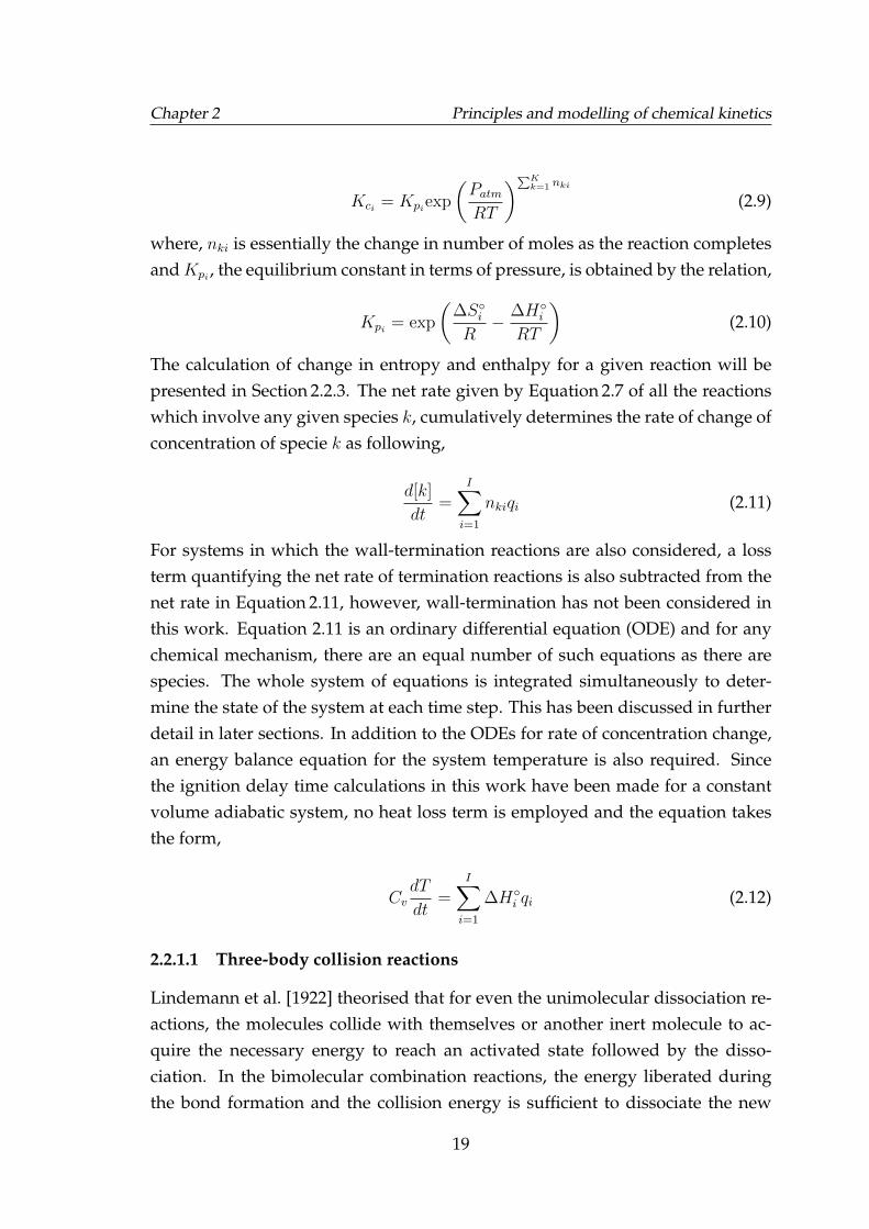
Chapter 2 Principles and modelling of chemical kinetics
Kci = Kpiexp
(PatmRT
)∑Kk=1 nki
(2.9)
where, nki is essentially the change in number of moles as the reaction completesandKpi , the equilibrium constant in terms of pressure, is obtained by the relation,
Kpi = exp
(∆S◦iR− ∆H◦i
RT
)(2.10)
The calculation of change in entropy and enthalpy for a given reaction will bepresented in Section 2.2.3. The net rate given by Equation 2.7 of all the reactionswhich involve any given species k, cumulatively determines the rate of change ofconcentration of specie k as following,
d[k]
dt=
I∑i=1
nkiqi (2.11)
For systems in which the wall-termination reactions are also considered, a lossterm quantifying the net rate of termination reactions is also subtracted from thenet rate in Equation 2.11, however, wall-termination has not been considered inthis work. Equation 2.11 is an ordinary differential equation (ODE) and for anychemical mechanism, there are an equal number of such equations as there arespecies. The whole system of equations is integrated simultaneously to deter-mine the state of the system at each time step. This has been discussed in furtherdetail in later sections. In addition to the ODEs for rate of concentration change,an energy balance equation for the system temperature is also required. Sincethe ignition delay time calculations in this work have been made for a constantvolume adiabatic system, no heat loss term is employed and the equation takesthe form,
CvdT
dt=
I∑i=1
∆H◦i qi (2.12)
2.2.1.1 Three-body collision reactions
Lindemann et al. [1922] theorised that for even the unimolecular dissociation re-actions, the molecules collide with themselves or another inert molecule to ac-quire the necessary energy to reach an activated state followed by the disso-ciation. In the bimolecular combination reactions, the energy liberated duringthe bond formation and the collision energy is sufficient to dissociate the new
19
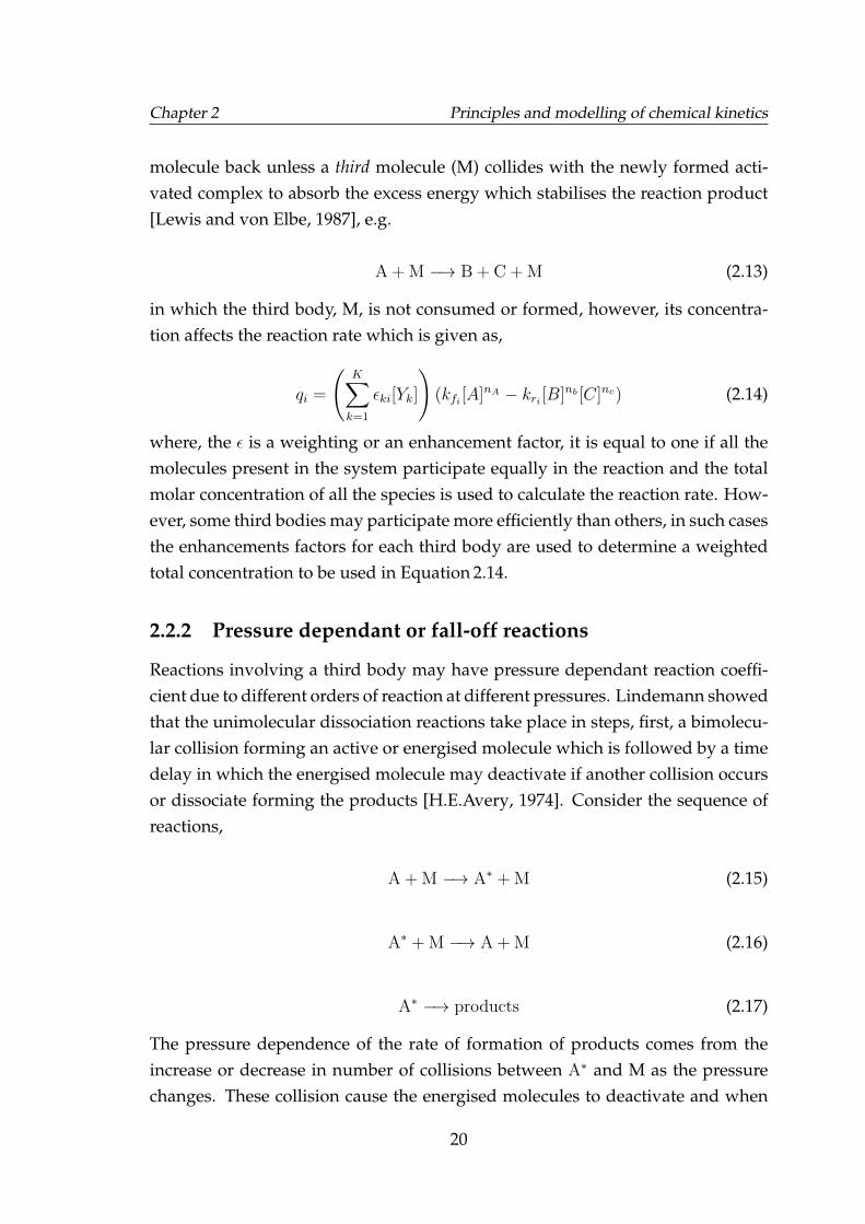
Chapter 2 Principles and modelling of chemical kinetics
molecule back unless a third molecule (M) collides with the newly formed acti-vated complex to absorb the excess energy which stabilises the reaction product[Lewis and von Elbe, 1987], e.g.
A + M −→ B + C + M (2.13)
in which the third body, M, is not consumed or formed, however, its concentra-tion affects the reaction rate which is given as,
qi =
(K∑k=1
εki[Yk]
)(kfi [A]nA − kri [B]nb [C]nc) (2.14)
where, the ε is a weighting or an enhancement factor, it is equal to one if all themolecules present in the system participate equally in the reaction and the totalmolar concentration of all the species is used to calculate the reaction rate. How-ever, some third bodies may participate more efficiently than others, in such casesthe enhancements factors for each third body are used to determine a weightedtotal concentration to be used in Equation 2.14.
2.2.2 Pressure dependant or fall-off reactions
Reactions involving a third body may have pressure dependant reaction coeffi-cient due to different orders of reaction at different pressures. Lindemann showedthat the unimolecular dissociation reactions take place in steps, first, a bimolecu-lar collision forming an active or energised molecule which is followed by a timedelay in which the energised molecule may deactivate if another collision occursor dissociate forming the products [H.E.Avery, 1974]. Consider the sequence ofreactions,
A + M −→ A∗ + M (2.15)
A∗ + M −→ A + M (2.16)
A∗ −→ products (2.17)
The pressure dependence of the rate of formation of products comes from theincrease or decrease in number of collisions between A∗ and M as the pressurechanges. These collision cause the energised molecules to deactivate and when
20
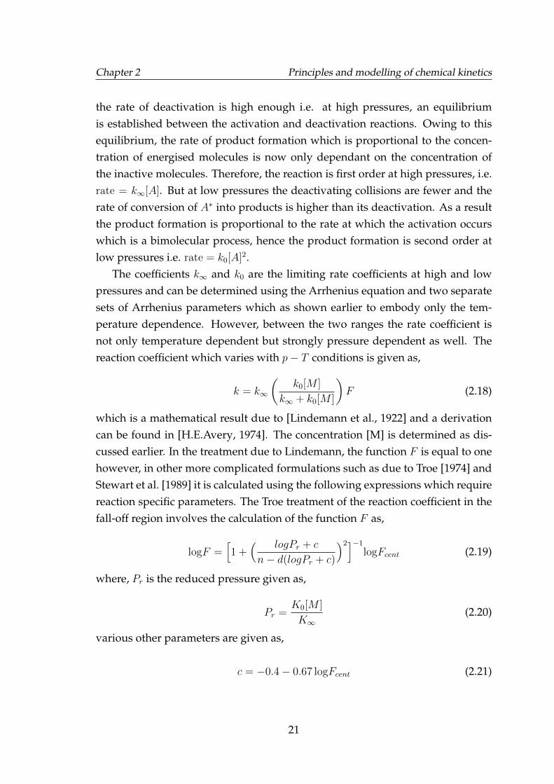
Chapter 2 Principles and modelling of chemical kinetics
the rate of deactivation is high enough i.e. at high pressures, an equilibriumis established between the activation and deactivation reactions. Owing to thisequilibrium, the rate of product formation which is proportional to the concen-tration of energised molecules is now only dependant on the concentration ofthe inactive molecules. Therefore, the reaction is first order at high pressures, i.e.rate = k∞[A]. But at low pressures the deactivating collisions are fewer and therate of conversion of A∗ into products is higher than its deactivation. As a resultthe product formation is proportional to the rate at which the activation occurswhich is a bimolecular process, hence the product formation is second order atlow pressures i.e. rate = k0[A]2.
The coefficients k∞ and k0 are the limiting rate coefficients at high and lowpressures and can be determined using the Arrhenius equation and two separatesets of Arrhenius parameters which as shown earlier to embody only the tem-perature dependence. However, between the two ranges the rate coefficient isnot only temperature dependent but strongly pressure dependent as well. Thereaction coefficient which varies with p− T conditions is given as,
k = k∞
(k0[M ]
k∞ + k0[M ]
)F (2.18)
which is a mathematical result due to [Lindemann et al., 1922] and a derivationcan be found in [H.E.Avery, 1974]. The concentration [M] is determined as dis-cussed earlier. In the treatment due to Lindemann, the function F is equal to onehowever, in other more complicated formulations such as due to Troe [1974] andStewart et al. [1989] it is calculated using the following expressions which requirereaction specific parameters. The Troe treatment of the reaction coefficient in thefall-off region involves the calculation of the function F as,
logF =[1 +
( logPr + c
n− d(logPr + c)
)2]−1
logFcent (2.19)
where, Pr is the reduced pressure given as,
Pr =K0[M ]
K∞(2.20)
various other parameters are given as,
c = −0.4− 0.67 logFcent (2.21)
21
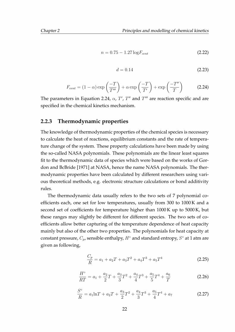
Chapter 2 Principles and modelling of chemical kinetics
n = 0.75− 1.27 logFcent (2.22)
d = 0.14 (2.23)
Fcent = (1− α) exp
(−TT ′′′
)+ α exp
(−TT ′
)+ exp
(−T ′′
T
)(2.24)
The parameters in Equation 2.24, α, T ′, T ′′ and T ′′′ are reaction specific and arespecified in the chemical kinetics mechanism.
2.2.3 Thermodynamic properties
The knowledge of thermodynamic properties of the chemical species is necessaryto calculate the heat of reactions, equilibrium constants and the rate of tempera-ture change of the system. These property calculations have been made by usingthe so-called NASA polynomials. These polynomials are the linear least squaresfit to the thermodynamic data of species which were based on the works of Gor-don and BcBride [1971] at NASA, hence the name NASA polynomials. The ther-modynamic properties have been calculated by different researchers using vari-ous theoretical methods, e.g. electronic structure calculations or bond additivityrules.
The thermodynamic data usually refers to the two sets of 7 polynomial co-efficients each, one set for low temperatures, usually from 300 to 1000 K and asecond set of coefficients for temperature higher than 1000 K up to 5000 K, butthese ranges may slightly be different for different species. The two sets of co-efficients allow better capturing of the temperature dependence of heat capacitymainly but also of the other two properties. The polynomials for heat capacity atconstant pressure, Cp, sensible enthalpy, H◦ and standard entropy, S◦ at 1 atm aregiven as following,
CpR
= a1 + a2T + a3T2 + a4T
3 + a5T4 (2.25)
H◦
RT= a1 +
a2
2T +
a3
3T 2 +
a4
4T 3 +
a5
5T 4 +
a6
T(2.26)
S◦
R= a1lnT + a2T +
a3
2T 2 +
a4
3T 3 +
a5
4T 4 + a7 (2.27)
22
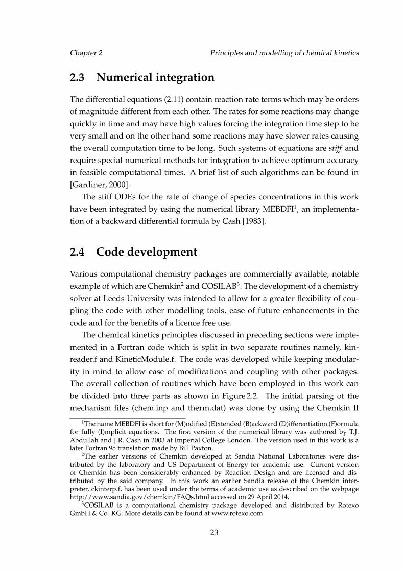
Chapter 2 Principles and modelling of chemical kinetics
2.3 Numerical integration
The differential equations (2.11) contain reaction rate terms which may be ordersof magnitude different from each other. The rates for some reactions may changequickly in time and may have high values forcing the integration time step to bevery small and on the other hand some reactions may have slower rates causingthe overall computation time to be long. Such systems of equations are stiff andrequire special numerical methods for integration to achieve optimum accuracyin feasible computational times. A brief list of such algorithms can be found in[Gardiner, 2000].
The stiff ODEs for the rate of change of species concentrations in this workhave been integrated by using the numerical library MEBDFI1, an implementa-tion of a backward differential formula by Cash [1983].
2.4 Code development
Various computational chemistry packages are commercially available, notableexample of which are Chemkin2 and COSILAB3. The development of a chemistrysolver at Leeds University was intended to allow for a greater flexibility of cou-pling the code with other modelling tools, ease of future enhancements in thecode and for the benefits of a licence free use.
The chemical kinetics principles discussed in preceding sections were imple-mented in a Fortran code which is split in two separate routines namely, kin-reader.f and KineticModule.f. The code was developed while keeping modular-ity in mind to allow ease of modifications and coupling with other packages.The overall collection of routines which have been employed in this work canbe divided into three parts as shown in Figure 2.2. The initial parsing of themechanism files (chem.inp and therm.dat) was done by using the Chemkin II
1The name MEBDFI is short for (M)odified (E)xtended (B)ackward (D)ifferentiation (F)ormulafor fully (I)mplicit equations. The first version of the numerical library was authored by T.J.Abdullah and J.R. Cash in 2003 at Imperial College London. The version used in this work is alater Fortran 95 translation made by Bill Paxton.
2The earlier versions of Chemkin developed at Sandia National Laboratories were dis-tributed by the laboratory and US Department of Energy for academic use. Current versionof Chemkin has been considerably enhanced by Reaction Design and are licensed and dis-tributed by the said company. In this work an earlier Sandia release of the Chemkin inter-preter, ckinterp.f, has been used under the terms of academic use as described on the webpagehttp://www.sandia.gov/chemkin/FAQs.html accessed on 29 April 2014.
3COSILAB is a computational chemistry package developed and distributed by RotexoGmbH & Co. KG. More details can be found at www.rotexo.com
23
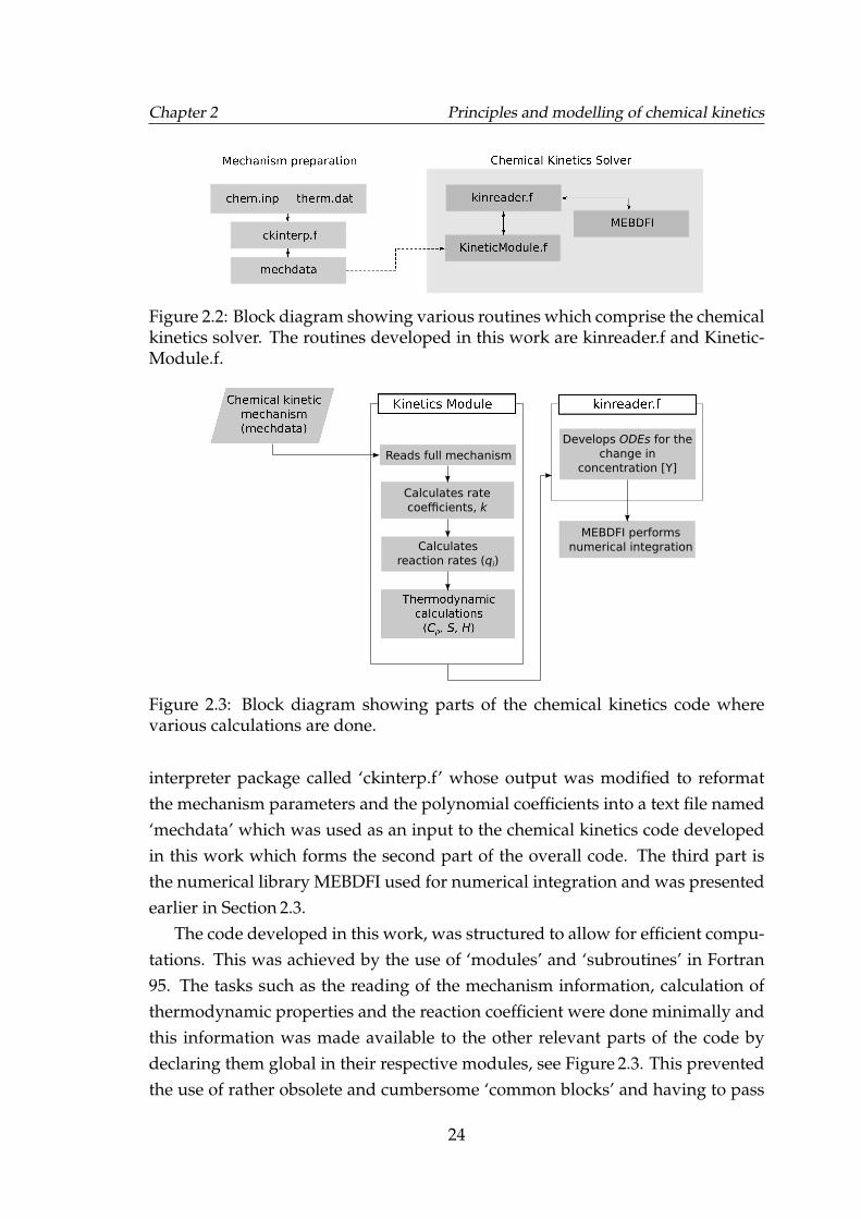
Chapter 2 Principles and modelling of chemical kinetics
ckinterp.f
chem.inp therm.dat
Figure 2.2: Block diagram showing various routines which comprise the chemicalkinetics solver. The routines developed in this work are kinreader.f and Kinetic-Module.f.
Reads full mechanism
Calculates rate
coefficients, k
Develops ODEs for the
change in
concentration [Y]
Calculates
reaction rates (qi)
MEBDFI performs
numerical integration
Chemical kinetic
mechanism
(mechdata)
Figure 2.3: Block diagram showing parts of the chemical kinetics code wherevarious calculations are done.
interpreter package called ‘ckinterp.f’ whose output was modified to reformatthe mechanism parameters and the polynomial coefficients into a text file named‘mechdata’ which was used as an input to the chemical kinetics code developedin this work which forms the second part of the overall code. The third part isthe numerical library MEBDFI used for numerical integration and was presentedearlier in Section 2.3.
The code developed in this work, was structured to allow for efficient compu-tations. This was achieved by the use of ‘modules’ and ‘subroutines’ in Fortran95. The tasks such as the reading of the mechanism information, calculation ofthermodynamic properties and the reaction coefficient were done minimally andthis information was made available to the other relevant parts of the code bydeclaring them global in their respective modules, see Figure 2.3. This preventedthe use of rather obsolete and cumbersome ‘common blocks’ and having to pass
24
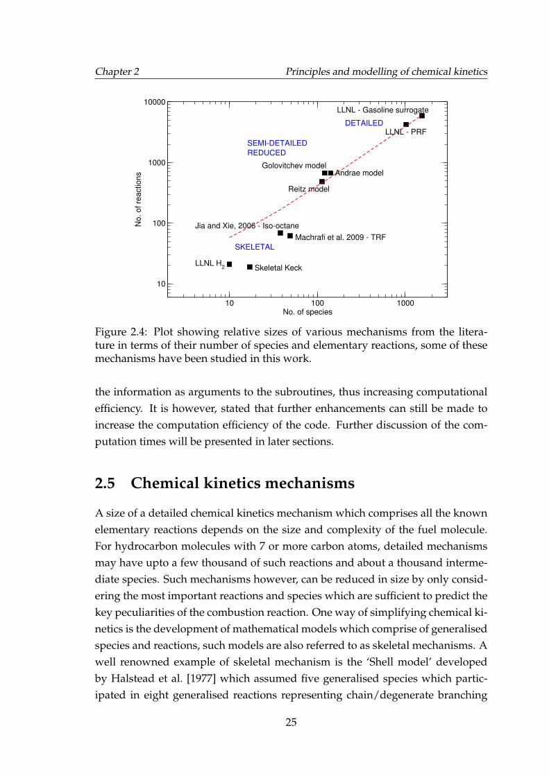
Chapter 2 Principles and modelling of chemical kinetics
10 100 1000No. of species
10
100
1000
10000
No. of re
actions
LLNL H2 Skeletal Keck
Machrafi et al. 2009 - TRF
Jia and Xie, 2006 - Iso-octane
Reitz model
Andrae modelGolovitchev model
LLNL - PRF
LLNL - Gasoline surrogate
DETAILED
SEMI-DETAILED
REDUCED
SKELETAL
Figure 2.4: Plot showing relative sizes of various mechanisms from the litera-ture in terms of their number of species and elementary reactions, some of thesemechanisms have been studied in this work.
the information as arguments to the subroutines, thus increasing computationalefficiency. It is however, stated that further enhancements can still be made toincrease the computation efficiency of the code. Further discussion of the com-putation times will be presented in later sections.
2.5 Chemical kinetics mechanisms
A size of a detailed chemical kinetics mechanism which comprises all the knownelementary reactions depends on the size and complexity of the fuel molecule.For hydrocarbon molecules with 7 or more carbon atoms, detailed mechanismsmay have upto a few thousand of such reactions and about a thousand interme-diate species. Such mechanisms however, can be reduced in size by only consid-ering the most important reactions and species which are sufficient to predict thekey peculiarities of the combustion reaction. One way of simplifying chemical ki-netics is the development of mathematical models which comprise of generalisedspecies and reactions, such models are also referred to as skeletal mechanisms. Awell renowned example of skeletal mechanism is the ‘Shell model’ developedby Halstead et al. [1977] which assumed five generalised species which partic-ipated in eight generalised reactions representing chain/degenerate branching
25
Chapter 2 Principles and modelling of chemical kinetics
and termination reactions. Separate sets of fitted Arrhenius parameters for PRFsof RON 70, 90 and 100, TRFs of RON 89.5 and 99.6 and 2-methyl-2hex-2-ene wereprovided. This mechanism formed the foundation for numerous important skele-tal mechanisms for alkanes. One of the important work on skeletal hydrocarbonmechanisms is of Cox and Cole [1985] who developed on the earlier works ofKnox [1967] and also the Shell model and proposed an alkane mechanism with15 reactions and 10 species. This model was further extended by Hu and Keck[1987] specifically for iso-octane, comprising of 18 reactions for low to high tem-perature chemistry in temperature range of 700 - 1300 K. Later extensions of Huand Keck model have long been used at Leeds University for autoignition pre-diction and are referred to as Skeletal Keck models. These extensions of the Keckmodel are [Chun et al., 1989], [Cowart et al., 1991] and [Nishiwaki et al., 2000].Examples of various mechanisms from the literature have been presented in Fig-ure 2.4 which shows a relative comparison of the complexity of these mechanismswhich can be arbitrarily grouped as detailed, semi-detailed or reduced and skele-tal mechanisms.
A comparison of the autoignition delay times predicted using these mecha-nisms is presented in Figure 2.5. It should be noted that these preliminary simu-lations in Figure 2.5 were done using Cosilab for the detailed and semi-detailedmechanisms; earlier Fortran implementations of the Skeletal Keck models wereused and the models [Machrafi et al., 2009] and [Jia and Xie, 2006] were explic-itly implemented in a Fortran code. The ignition delays for iso-octane shown inthe figure indicate that simpler skeletal and heavily reduced mechanisms deviatesubstantially from the shock tube measurements. The Skeletal Keck mechanismsare only reasonable in predicting at the lowest temperatures which are more rel-evant to engine autoignition, however, model inaccuracies have been found toresult in unreliable autoignition predictions as demonstrated in Chapter 6. More-over, such skeletal mechanisms are optimised for a specific fuel and it is not pos-sible to account for different RON and MON of the fuels. The most detailedmechanism in this comparison, the PRF mechanism proposed in [Curran et al.,1998b] and named as LLNL - PRF in Figure 2.4 performs well but no better thanthe three reduced mechanisms. These are the Andrae [Andrae and Head, 2009]model which comprises 144 species and 673 reactions, the Golovitchev [Huanget al., 2010] model comprising 121 species and 681 reactions and the Reitz [Raand Reitz, 2011] model also known as MultiChem model which comprises 113species and 487 reactions.
26
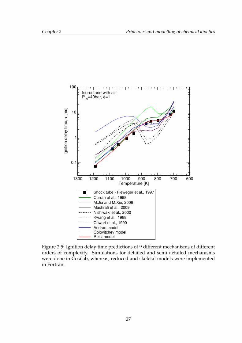
Chapter 2 Principles and modelling of chemical kinetics
6007008009001000110012001300Temperature [K]
0.1
1
10
100
Ign
itio
n d
ela
y t
ime
, τ
[ms]
Shock tube - Fieweger et al., 1997
Curran et al., 1998
M.Jia and M.Xie, 2006
Machrafi et al., 2009
Nishiwaki et al., 2000
Kwang et al., 1988
Cowart et al., 1990
Andrae modelGolovitchev modelReitz model
Iso-octane with airP
ini=40bar, φ=1
Figure 2.5: Ignition delay time predictions of 9 different mechanisms of differentorders of complexity. Simulations for detailed and semi-detailed mechanismswere done in Cosilab, whereas, reduced and skeletal models were implementedin Fortran.
27
Chapter 2 Principles and modelling of chemical kinetics
It was found that the three reduced mechanisms are a better choice over moredetailed or simpler Skeletal mechanisms because they comprise pathways for keygasoline surrogate components which can be used as representatives of the ma-jor constituent hydrocarbon families of the gasoline. These mechanisms are alsoappropriately sized which results in feasible computational times. Most impor-tantly, these mechanisms are able to predict ignition delay times with appreciableaccuracy for a variety of operating conditions and equivalence ratios, as will bedemonstrated through comparisons with experimental measurements from theliterature in later sections. A brief introduction of these mechanisms is givenhere.
2.5.1 Andrae model
The mechanism used in this work can be obtained as supplementary materialto the paper [Andrae and Head, 2009]. Andrae and partners developed theirgasoline surrogate mechanism by extending an earlier tri-component TRF mech-anism, [Andrae et al., 2007]; the resulting multi-component mechanism was firstintroduced in [Andrae, 2008]. Andrae’s TRF mechanism was essentially a cou-pling of highly reduced PRF submechanisms with a relatively detailed toluenemechanism and expectedly, his extension work to produce the gasoline surro-gate mechanism involved further addition to the toluene mechanism of the keyreactions of phenyl (C6H5) whose participant species were observed at lean condi-tions in shock tube experiments, see [Andrae, 2008] and references therein. Thisallowed improvements in lean combustion predictions demonstrated by HCCIpredictions. Andrae considered diisobutylene1 (DIB) to be an important olefinand a suitable surrogate component and included its reaction pathways and ratedata from the work of Metcalfe et al. [2007] who studied DIB as a candidate fordiesel surrogate. DIB was given importance because of its similar structure tothat of iso-octane which means it can be an important intermediary to iso-octaneoxidation. It was therefore, proposed to be formed in the reaction,
C8H17 + O2 ←→ C8H16 + HO2 (2.28)
and decomposed irreversibly to form iso-butene (IC4H8), an important olefin. Thesubmechanism for ethanol was based on the works of Marinov [1999] as do most
1Diisobutylene is a mixture of two conjugate olefins of iso-octane, which are 2,4,4-trimethyl-1-(and-2)-pentene with a molecular formula of C8H16.
28
Chapter 2 Principles and modelling of chemical kinetics
of the ethanol mechanisms as limited reaction rate data is available for its oxida-tion.
Although various works report good agreement predictions of autoignitiondelays of DIB and its blends, however, one drawback for choosing DIB as anolefin representative for gasoline is its high molecular weight. Majority of olefincontent in gasoline is composed of smaller molecules and as a result surrogateformulation becomes challenging if matching the hydrogen to carbon ratio (H/C)and molecular weights of the surrogate and gasoline is desired. Moreover, theoctane numbers of DIB are:
2,4,4-trimethyl-1-pentene 106 RON 86.5 MON2,4,4-trimethyl-2-pentene 103.5 RON 86.2 MON
which are considerably high compared to smaller olefins. This notion will be fur-ther explored in sections covering gasoline surrogate formulation. But it is worthmentioning it here because, even though Andrae model performs well and it hasacted as basis for a number of recent reduced gasoline surrogates with similarconstituents, e.g. [Wang et al., 2013] and [Zhong and Zheng, 2014], it appearsthat original thinking on prioritising olefins for specifically gasoline surrogates,is lacking.
2.5.2 Golovitchev model
The Golovitchev mechanism is also a multicomponent gasoline surrogate mech-anism which was developed hierarchically by building on submechanisms forH2, CH3, CH2O, CH3CHO, CO, larger alkanes, alkenes and finally incorporatingpathways for toluene. That resulting mechanism was without ethanol and it wasextensively validated for the autoigniton predictions of the submechanisms ontheir own as well as for blends of the main components i.e. the gasoline sur-rogates at different conditions which can be found in [Ogink and Golovitchev,2002] and [Ogink, 2004]. The mechanism was further extended by the additionof ethanol pathways which also consisted of reactions for dimethyl-ether (DME)and revalidated against a large set of ignition delay time data and laminar burn-ing velocities as well [Huang et al., 2010].
29
Chapter 2 Principles and modelling of chemical kinetics
2.5.3 Reitz model
The Reitz model otherwise known as MultiChem is a reduced multicomponentmechanism which has submechanisms for a number of species which qualify asboth gasoline and diesel surrogates, e.g. dimethyl-ether, methyl butanoate andn-tetradecane which are present in addition to the usual components. The mech-anism development rather seems to follow a top-down reduction approach frommore detailed mechanisms, resulting in a small mechanism of 113 species and487 reactions, smaller than the Andrae and the Golovitchev models.
MultiChem evolved from their earlier PRF mechanism [Ra and Reitz, 2008]which was reduced from the detailed works of [Curran et al., 1998a] and [Curranet al., 2002]. The mechanism was reported to perform remarkably well for PRFsfor their 0-D autoignition delays and CFD modelling of HCCI and this also beenseen in this work that the PRF predictions of the Reitz model are superior withsome exceptions. The pathways for PRF oxidation are not greatly different for thethree mechanisms, the difference is mostly in the reaction coefficients which areoptimised in each mechanism, however, more so in Reitz model than others. Themechanism for toluene in the Reitz model is based on the works of [Bounaceuret al., 2005] and [Andrae et al., 2007]. The ethanol mechanism is based on the de-tailed mechanism of Marinov [1999] which was reduced through sensitivity andflux analyses. Ra and Reitz [2011] also included submechanism for cyclo-hexane,an important naphthene component of gasoline, although not as abundant ascyclo-pentane [Pera and Knop, 2012].
2.6 Code validation
The chemistry solver developed as part of this work was first compared to twoother packages, Chemkin II and Cosilab. Some of the comparisons of ignitiondelay times of iso-octane, n-heptane and toluene obtained by the three reducedmechanisms have been presented in Figures 2.6 to 2.8 which show that the igni-tion delay times calculated using the Leeds Chemistry Solver are very close tothe calculations of other two packages. Minute differences can be seen which canbe attributed to the different numerical schemes used by these packages, round-ing of the digits and possibly interpolation of thermodynamic data instead of re-calculation at each time-step by Chemkin II and Cosilab which was not done inLeeds Chemistry Solver as it did not offer any perceptible computational benefit.
30
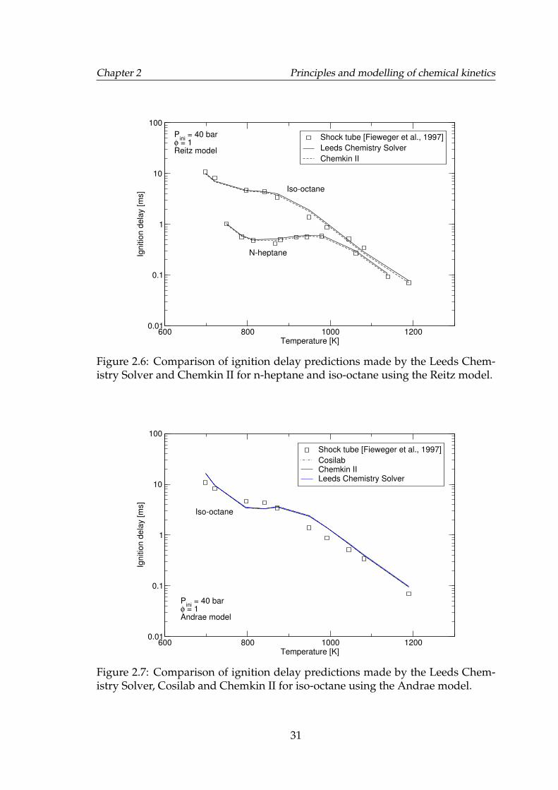
Chapter 2 Principles and modelling of chemical kinetics
600 800 1000 1200Temperature [K]
0.01
0.1
1
10
100
Ignitio
n d
ela
y [m
s]
Shock tube [Fieweger et al., 1997]
Leeds Chemistry Solver
Chemkin II
Pini
= 40 barφ = 1Reitz model
Iso-octane
N-heptane
Figure 2.6: Comparison of ignition delay predictions made by the Leeds Chem-istry Solver and Chemkin II for n-heptane and iso-octane using the Reitz model.
600 800 1000 1200Temperature [K]
0.01
0.1
1
10
100
Ignitio
n d
ela
y [m
s]
Shock tube [Fieweger et al., 1997]
CosilabChemkin IILeeds Chemistry Solver
Pini
= 40 barφ = 1Andrae model
Iso-octane
Figure 2.7: Comparison of ignition delay predictions made by the Leeds Chem-istry Solver, Cosilab and Chemkin II for iso-octane using the Andrae model.
31
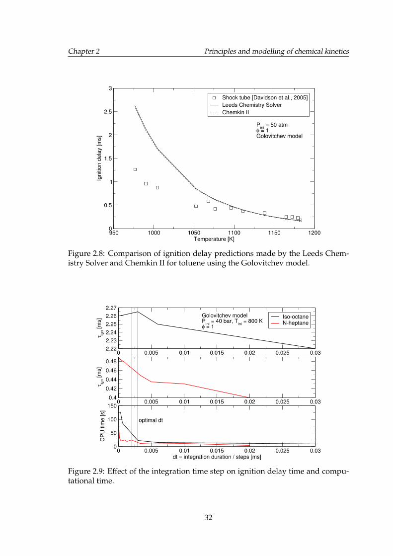
Chapter 2 Principles and modelling of chemical kinetics
950 1000 1050 1100 1150 1200Temperature [K]
0
0.5
1
1.5
2
2.5
3
Ign
itio
n d
ela
y [
ms]
Shock tube [Davidson et al., 2005]
Leeds Chemistry Solver
Chemkin II
Pini
= 50 atmφ = 1Golovitchev model
Figure 2.8: Comparison of ignition delay predictions made by the Leeds Chem-istry Solver and Chemkin II for toluene using the Golovitchev model.
0 0.005 0.01 0.015 0.02 0.025 0.032.22
2.23
2.24
2.25
2.26
2.27
τ ign [m
s]
0 0.005 0.01 0.015 0.02 0.025 0.030.4
0.42
0.44
0.46
0.48
τ ign [m
s]
0 0.005 0.01 0.015 0.02 0.025 0.03dt = integration duration / steps [ms]
0
50
100
150
CP
U tim
e [s]
Iso-octaneN-heptane
Golovitchev modelP
ini = 40 bar, T
ini = 800 K
φ = 1
optimal dt
Figure 2.9: Effect of the integration time step on ignition delay time and compu-tational time.
32
Chapter 2 Principles and modelling of chemical kinetics
The time duration of a simulation was found to be dependant on the integra-tion time step and also the stiffness of the mechanism. The numerical library,MEBDFI, uses an internal dynamic time step, however, the duration of integra-tion and the integration interval or the step size must be specified. A smallertime step, dt, increases the computational time and a too coarse a time step causeslarger truncation errors. A compromise must therefore be reached between accu-racy and computational time. The stiffness of the mechanism plays a role whenall or a large number of reactions have a non-zero net reaction rate which forcesthe internal dynamic stepping to be refined which increases the computationaltime. Simulations of blends are therefore expected to be longer than neat fuels aspresence of difference species right from the beginning would initiate reactionsearlier on increasing stiffness. Figure 2.9 shows ignition delay times, τign, for iso-octane and n-heptane at same initial p − T condition but the time step has beenchanged. As the time step is decreased, τign starts to stabilise, see iso-octane curvespecifically, however, correspondingly the computation time increases manifolds.A time step of roughly 0.025 ms appears to be a feasible value at which the com-putational times are between 20 to 30 s acceptable for a single constant volumeautoignition simulation. When coupled with engine modelling, the computa-tional time will also depend on engine speed and in this work is found to be ofthe order of 1 minute per cycle.
2.7 Autoignition simulation results
It was of an obvious interest to first study the autoignition predictions of the threereduced mechanisms. Constant volume, 0-D, autoignition simulations were car-ried out by using the Leeds Chemistry Solver for the four main gasoline surro-gate components, iso-octane, n-heptane, toluene and ethanol. Simulations donefor a range of temperatures, were compared to shock tube measurements at lowpressures (10 - 13 bar) and high pressures (40 - 50 bar) for stoichiometric air-fuelmixtures as these are of relevance to SI engines. The low pressure comparisonshave been presented in Figure 2.10 and high pressure comparisons in Figure 2.11.For SI engine autoignition, the temperatures upto about 850 K or 1000/T > 1.15
are important. The model accuracy at these temperatures is indeed of great sig-nificance, however, accurate predictions at higher temperatures are crucial too asblending may cause the otherwise high temperature channels for certain compo-nents to become active at lower temperatures, e.g. for toluene and ethanol when
33
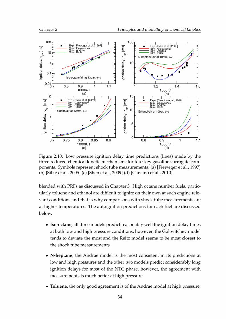
Chapter 2 Principles and modelling of chemical kinetics
0.7 0.8 0.9 1 1.11000K/T (a)
0.01
0.1
1
10
100Ig
nitio
n d
ela
y,
τ ign [
ms] Exp - Fieweger et al. [1997]
Sim - GolovitchevSim - AndraeSim - Reitz
1 1.2 1.4 1.61000K/T (b)
1
10
100
Ign
itio
n d
ela
y,
τ ign [
ms] Exp - Silke at al. [2005]
Sim - GolovitchevSim - AndraeSim - Reitz
0.7 0.75 0.8 0.85 0.91000K/T (c)
1
2
Ign
itio
n d
ela
y,
τ ign [
ms] Exp - Shen et al. [2009]
Sim - GolovitchevSim - AndraeSim - Reitz
0.8 0.9 1 1.11000K/T (d)
0
5
10
15
Ign
itio
n d
ela
y,
τ ign [
ms]
Exp - [Cancino et al., 2010]Sim - GolovitchevSim - AndraeSim - Reitz
Toluene/air at 12atm, φ=1
Iso-octane/air at 13bar, φ=1
N-heptane/air at 10atm, φ=1
Ethanol/air at 10bar, φ=1
Figure 2.10: Low pressure ignition delay time predictions (lines) made by thethree reduced chemical kinetic mechanisms for four key gasoline surrogate com-ponents. Symbols represent shock tube measurements; (a) [Fieweger et al., 1997](b) [Silke et al., 2005] (c) [Shen et al., 2009] (d) [Cancino et al., 2010].
blended with PRFs as discussed in Chapter 3. High octane number fuels, partic-ularly toluene and ethanol are difficult to ignite on their own at such engine rele-vant conditions and that is why comparisons with shock tube measurements areat higher temperatures. The autoignition predictions for each fuel are discussedbelow.
• Iso-octane, all three models predict reasonably well the ignition delay timesat both low and high pressure conditions, however, the Golovitchev modeltends to deviate the most and the Reitz model seems to be most closest tothe shock tube measurements.
• N-heptane, the Andrae model is the most consistent in its predictions atlow and high pressures and the other two models predict considerably longignition delays for most of the NTC phase, however, the agreement withmeasurements is much better at high pressure.
• Toluene, the only good agreement is of the Andrae model at high pressure.
34
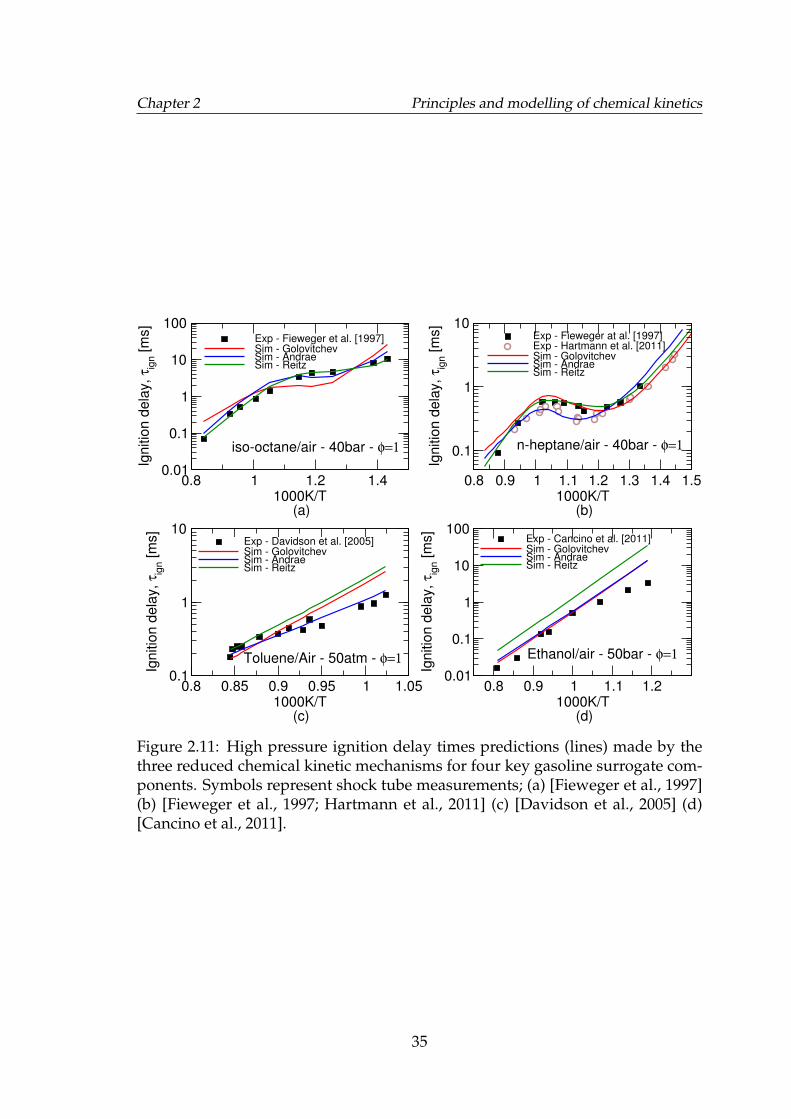
Chapter 2 Principles and modelling of chemical kinetics
0.8 1 1.2 1.41000K/T (a)
0.01
0.1
1
10
100
Ignitio
n d
ela
y,
τ ign [m
s]
Exp - Fieweger et al. [1997]Sim - GolovitchevSim - AndraeSim - Reitz
0.8 0.9 1 1.1 1.2 1.3 1.4 1.51000K/T (b)
0.1
1
10
Ignitio
n d
ela
y,
τ ign [m
s]
Exp - Fieweger at al. [1997]Exp - Hartmann et al. [2011]Sim - GolovitchevSim - AndraeSim - Reitz
0.8 0.85 0.9 0.95 1 1.051000K/T (c)
0.1
1
10
Ignitio
n d
ela
y,
τ ign [m
s]
Exp - Davidson et al. [2005]Sim - GolovitchevSim - AndraeSim - Reitz
0.8 0.9 1 1.1 1.21000K/T (d)
0.01
0.1
1
10
100
Ignitio
n d
ela
y,
τ ign [m
s]
Exp - Cancino et al. [2011]Sim - GolovitchevSim - AndraeSim - Reitz
Toluene/Air - 50atm - φ=1
iso-octane/air - 40bar - φ=1 n-heptane/air - 40bar - φ=1
Ethanol/air - 50bar - φ=1
Figure 2.11: High pressure ignition delay times predictions (lines) made by thethree reduced chemical kinetic mechanisms for four key gasoline surrogate com-ponents. Symbols represent shock tube measurements; (a) [Fieweger et al., 1997](b) [Fieweger et al., 1997; Hartmann et al., 2011] (c) [Davidson et al., 2005] (d)[Cancino et al., 2011].
35
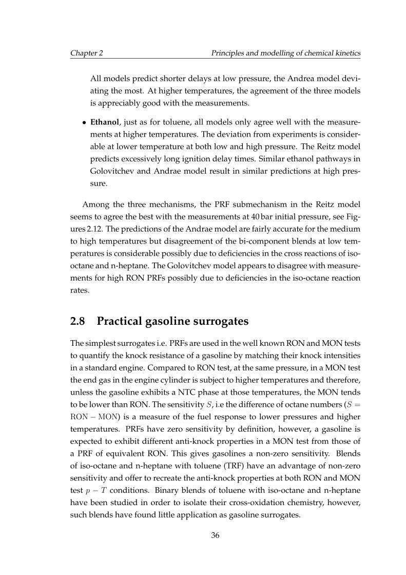
Chapter 2 Principles and modelling of chemical kinetics
All models predict shorter delays at low pressure, the Andrea model devi-ating the most. At higher temperatures, the agreement of the three modelsis appreciably good with the measurements.
• Ethanol, just as for toluene, all models only agree well with the measure-ments at higher temperatures. The deviation from experiments is consider-able at lower temperature at both low and high pressure. The Reitz modelpredicts excessively long ignition delay times. Similar ethanol pathways inGolovitchev and Andrae model result in similar predictions at high pres-sure.
Among the three mechanisms, the PRF submechanism in the Reitz modelseems to agree the best with the measurements at 40 bar initial pressure, see Fig-ures 2.12. The predictions of the Andrae model are fairly accurate for the mediumto high temperatures but disagreement of the bi-component blends at low tem-peratures is considerable possibly due to deficiencies in the cross reactions of iso-octane and n-heptane. The Golovitchev model appears to disagree with measure-ments for high RON PRFs possibly due to deficiencies in the iso-octane reactionrates.
2.8 Practical gasoline surrogates
The simplest surrogates i.e. PRFs are used in the well known RON and MON teststo quantify the knock resistance of a gasoline by matching their knock intensitiesin a standard engine. Compared to RON test, at the same pressure, in a MON testthe end gas in the engine cylinder is subject to higher temperatures and therefore,unless the gasoline exhibits a NTC phase at those temperatures, the MON tendsto be lower than RON. The sensitivity S, i.e the difference of octane numbers (S =
RON−MON) is a measure of the fuel response to lower pressures and highertemperatures. PRFs have zero sensitivity by definition, however, a gasoline isexpected to exhibit different anti-knock properties in a MON test from those ofa PRF of equivalent RON. This gives gasolines a non-zero sensitivity. Blendsof iso-octane and n-heptane with toluene (TRF) have an advantage of non-zerosensitivity and offer to recreate the anti-knock properties at both RON and MONtest p − T conditions. Binary blends of toluene with iso-octane and n-heptanehave been studied in order to isolate their cross-oxidation chemistry, however,such blends have found little application as gasoline surrogates.
36
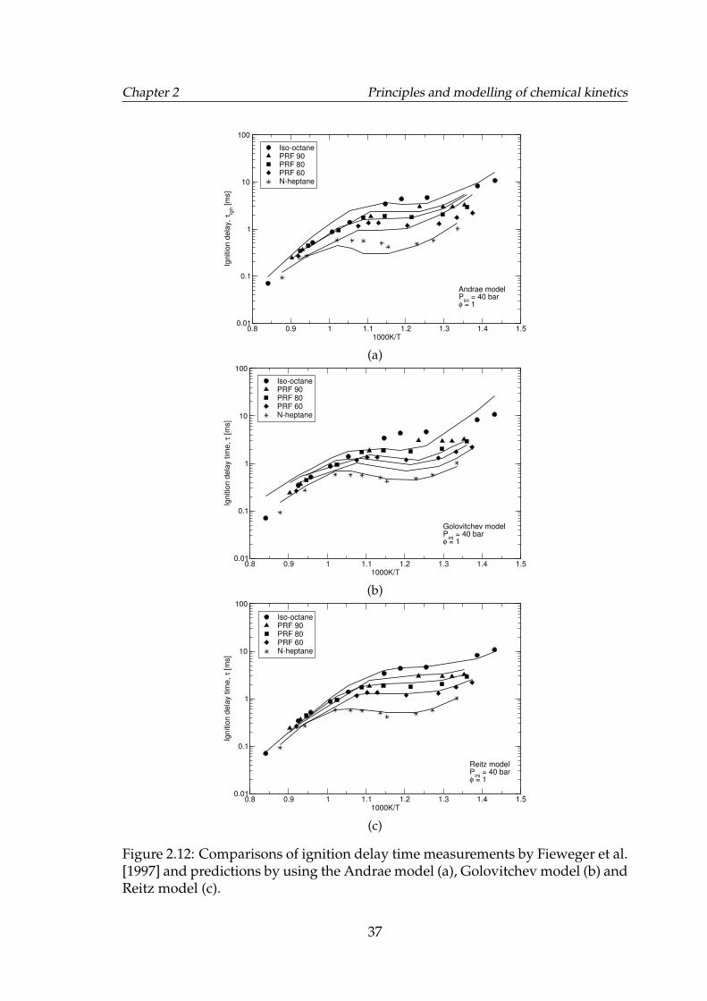
Chapter 2 Principles and modelling of chemical kinetics
0.8 0.9 1 1.1 1.2 1.3 1.4 1.51000K/T
0.01
0.1
1
10
100
Ignitio
n d
ela
y,
τ ign [m
s]
Iso-octanePRF 90PRF 80PRF 60N-heptane
Andrae modelP
ini = 40 bar
φ = 1
(a)
0.8 0.9 1 1.1 1.2 1.3 1.4 1.51000K/T
0.01
0.1
1
10
100
Ign
itio
n d
ela
y t
ime
, τ
[ms]
Iso-octanePRF 90PRF 80PRF 60N-heptane
Golovitchev modelP
ini = 40 bar
φ = 1
(b)
0.8 0.9 1 1.1 1.2 1.3 1.4 1.51000K/T
0.01
0.1
1
10
100
Ign
itio
n d
ela
y t
ime
, τ
[ms]
Iso-octanePRF 90PRF 80PRF 60N-heptane
Reitz modelP
ini = 40 bar
φ = 1
(c)
Figure 2.12: Comparisons of ignition delay time measurements by Fieweger et al.[1997] and predictions by using the Andrae model (a), Golovitchev model (b) andReitz model (c).
37
Chapter 2 Principles and modelling of chemical kinetics
Iso-octane n-heptane Toluene Ethanol Olefin RON/MON Reference% by volume
63 17 20 - - 86.6/84.2* Gauthier et al. [2004]69 17 14 - - 85.7/84.6* Gauthier et al. [2004]62 18 - 20 - 95.1/89.5 Fikri et al. [2008]25 20 45.0 - 10 (DIB**) 94.6/85 Fikri et al. [2008]
37.8 10.2 12 40 - 98.75§ Cancino et al. [2009]30 22 25 10 13 (DIB) - Cancino et al. [2009]57 16 23 - 4 (C5H10−2) 91/83est. Mehl et al. [2011]
* determined by Knop et al. [2014]** diisobutylene (C8H16)est. estimated values§ estimated value, see Cancino et al. [2009]
Table 2.1: Volumetric composition of various gasoline surrogate blends found inthe literature for which extensive shock tube and RCM measurements have beenmade.
Use of iso-octane and n-heptane as components of a surrogate is hardly avoid-able as they represent linear and branched alkanes which are major gasoline com-ponents. Besides, the chemistry leading to their auto-ignition is relatively wellunderstood. However, gasoline does not consists only of alkanes. Thus, EN228,the European standard for gasoline specifies aromatic content of up to 35% byvolume, it also allows 5% ethanol by volume. Therefore, it seems natural to seekgasoline surrogates going beyond PRFs and TRFs which contain compounds ap-proximating various families of hydrocarbons present in the gasoline.
Various surrogates, TRFs as well as blends containing olefins and oxygenates,particularly ethanol, have been studied for their autoigntion properties in rapidcompression machines, shock tubes and HCCI engines and list of such surrogatesis presented in Table 2.1. Gauthier et al. [2004] performed a fairly comprehensiveshock tube study of two TRFs for p−T conditions of 12 - 25 atm and 45 - 60 atm at850 - 1280 K temperatures. The two TRFs were proposed to approximate a stan-dard research gasoline, RD387; with an anti knock index (AKI = RON+MON
2) of 87.
The measurements demonstrated similarities between the autoignition character-istics of the surrogates and their gasoline. Kukkadapu et al. [2013] further inves-tigated one of the TRF formulation proposed in [Gauthier et al., 2004]; this sur-rogate is referred to as Gauthier TRF-A (iso-octane 63%, n-heptane 17%, toluene20% by volume). Using Mehl et al. [2011] approach (described in subsequentparagraph) they also over-estimated the sensitivity of the Gauthier-A TRF to be6 points with RON/MON of 89.5/83.5. However, the RON and MON of the twoGauthier TRFs were later determined by Knop et al. [2014] and the AKI of the sur-rogates were found to be lower than 87, see Table 2.1. But, even more importantly,the sensitivity S of the two TRFs was found to be much lower than the usual gaso-
38
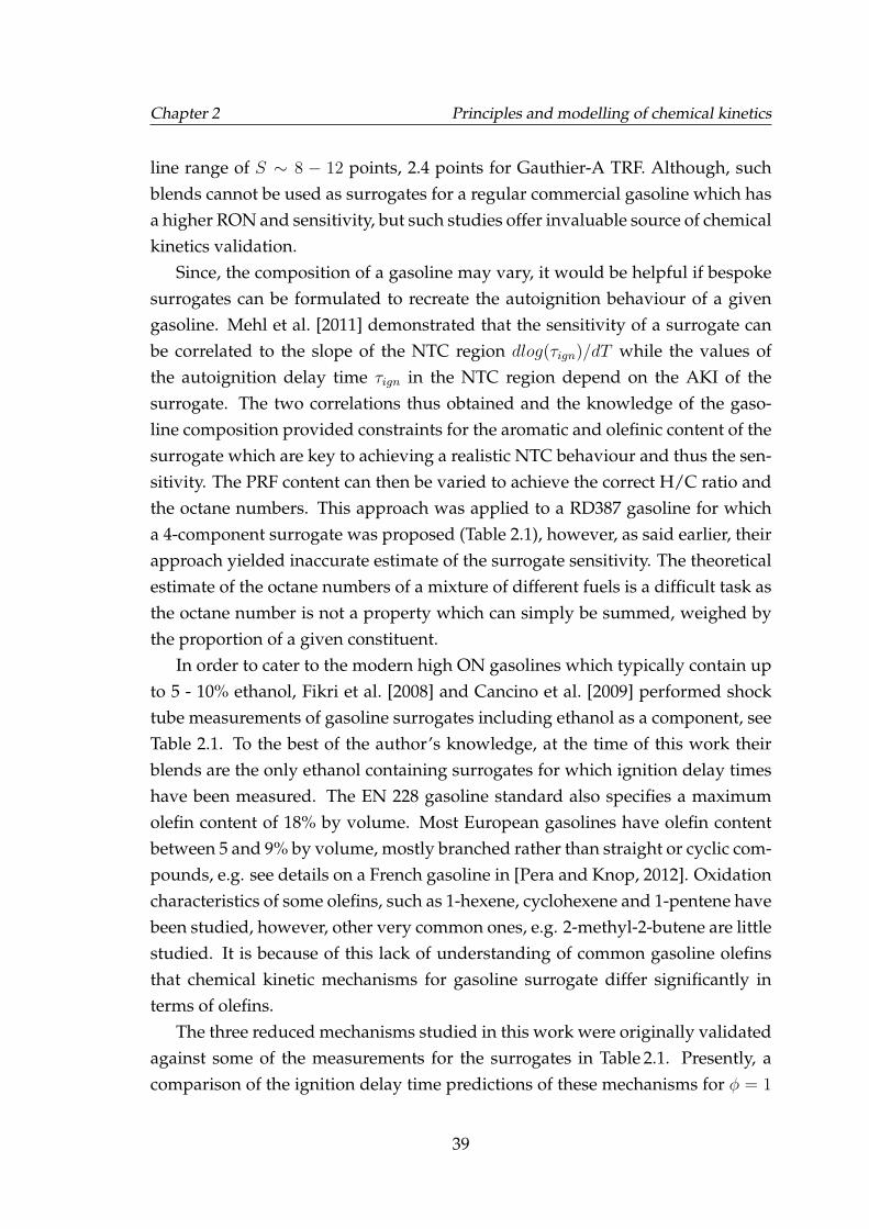
Chapter 2 Principles and modelling of chemical kinetics
line range of S ∼ 8 − 12 points, 2.4 points for Gauthier-A TRF. Although, suchblends cannot be used as surrogates for a regular commercial gasoline which hasa higher RON and sensitivity, but such studies offer invaluable source of chemicalkinetics validation.
Since, the composition of a gasoline may vary, it would be helpful if bespokesurrogates can be formulated to recreate the autoignition behaviour of a givengasoline. Mehl et al. [2011] demonstrated that the sensitivity of a surrogate canbe correlated to the slope of the NTC region dlog(τign)/dT while the values ofthe autoignition delay time τign in the NTC region depend on the AKI of thesurrogate. The two correlations thus obtained and the knowledge of the gaso-line composition provided constraints for the aromatic and olefinic content of thesurrogate which are key to achieving a realistic NTC behaviour and thus the sen-sitivity. The PRF content can then be varied to achieve the correct H/C ratio andthe octane numbers. This approach was applied to a RD387 gasoline for whicha 4-component surrogate was proposed (Table 2.1), however, as said earlier, theirapproach yielded inaccurate estimate of the surrogate sensitivity. The theoreticalestimate of the octane numbers of a mixture of different fuels is a difficult task asthe octane number is not a property which can simply be summed, weighed bythe proportion of a given constituent.
In order to cater to the modern high ON gasolines which typically contain upto 5 - 10% ethanol, Fikri et al. [2008] and Cancino et al. [2009] performed shocktube measurements of gasoline surrogates including ethanol as a component, seeTable 2.1. To the best of the author’s knowledge, at the time of this work theirblends are the only ethanol containing surrogates for which ignition delay timeshave been measured. The EN 228 gasoline standard also specifies a maximumolefin content of 18% by volume. Most European gasolines have olefin contentbetween 5 and 9% by volume, mostly branched rather than straight or cyclic com-pounds, e.g. see details on a French gasoline in [Pera and Knop, 2012]. Oxidationcharacteristics of some olefins, such as 1-hexene, cyclohexene and 1-pentene havebeen studied, however, other very common ones, e.g. 2-methyl-2-butene are littlestudied. It is because of this lack of understanding of common gasoline olefinsthat chemical kinetic mechanisms for gasoline surrogate differ significantly interms of olefins.
The three reduced mechanisms studied in this work were originally validatedagainst some of the measurements for the surrogates in Table 2.1. Presently, acomparison of the ignition delay time predictions of these mechanisms for φ = 1
39
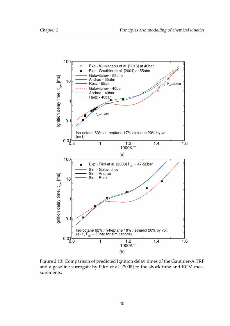
Chapter 2 Principles and modelling of chemical kinetics
0.8 1 1.2 1.4 1.61000K/T
0.01
0.1
1
10
100Ig
nitio
n d
ela
y t
ime
, τ ig
n [
ms]
Exp - Kukkadapu et al. [2013] at 40bar
Exp - Gauthier et al. [2004] at 55atm
Golovitchev - 55atmAndrae - 55atmReitz - 55atm
Iso-octane 63% / n-heptane 17% / toluene 20% by vol.(φ=1)
Pini
=40bar
Pini
=55atm
Golovitchev - 40barAndrae - 40barReitz - 40bar
(a)
0.8 1 1.2 1.4 1.61000K/T
0.01
0.1
1
10
100
Ign
itio
n d
ela
y t
ime
, τ ig
n [
ms]
Exp - Fikri et al. [2008] Pini
= 47-52bar
Sim - GolovitchevSim - AndraeSim - Reitz
Iso-octane 62% / n-heptane 18% / ethanol 20% by vol.(φ=1, P
ini = 50bar for simulations)
(b)
Figure 2.13: Comparison of predicted Ignition delay times of the Gauthier-A TRFand a gasoline surrogate by Fikri et al. [2008] to the shock tube and RCM mea-surements.
40
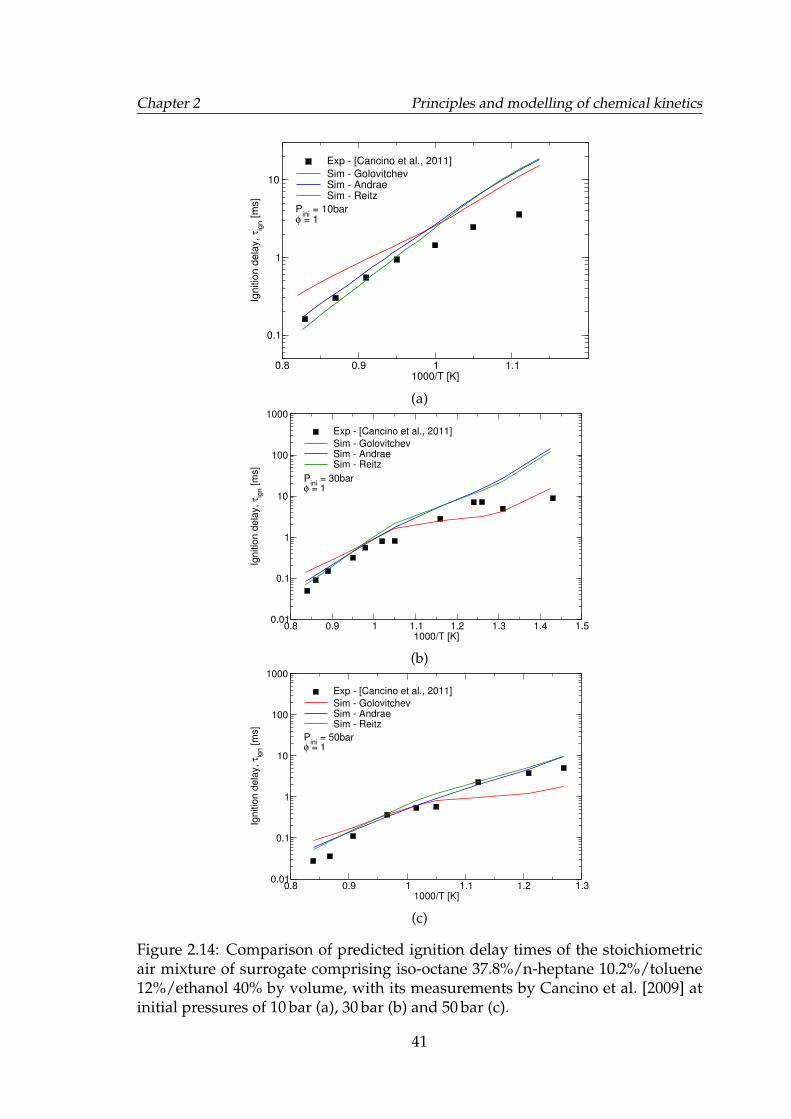
Chapter 2 Principles and modelling of chemical kinetics
0.8 0.9 1 1.11000/T [K]
0.1
1
10
Ignitio
n d
ela
y,
τ ign [m
s]
Exp - [Cancino et al., 2011]
Sim - GolovitchevSim - AndraeSim - Reitz
Pini
= 10barφ = 1
(a)
0.8 0.9 1 1.1 1.2 1.3 1.4 1.51000/T [K]
0.01
0.1
1
10
100
1000
Ignitio
n d
ela
y,
τ ign [m
s]
Exp - [Cancino et al., 2011]
Sim - GolovitchevSim - AndraeSim - Reitz
Pini
= 30barφ = 1
(b)
0.8 0.9 1 1.1 1.2 1.31000/T [K]
0.01
0.1
1
10
100
1000
Ignitio
n d
ela
y,
τ ign [m
s]
Exp - [Cancino et al., 2011]
Sim - GolovitchevSim - AndraeSim - Reitz
Pini
= 50barφ = 1
(c)
Figure 2.14: Comparison of predicted ignition delay times of the stoichiometricair mixture of surrogate comprising iso-octane 37.8%/n-heptane 10.2%/toluene12%/ethanol 40% by volume, with its measurements by Cancino et al. [2009] atinitial pressures of 10 bar (a), 30 bar (b) and 50 bar (c).
41
Chapter 2 Principles and modelling of chemical kinetics
at high pressure has been done. Simulations of the surrogates made up of dif-ferent components and compositions have been made and the results have beenpresented in Figures 2.13 and 2.14.
2.9 Gasoline surrogate formulation
The approach to surrogate formulation depends on its modelling application. Anumber of physical and chemical properties of the target fuel can be reproducedin the surrogate such as the distillation curve, RON, MON, stoichiometric air tofuel ratio, molecular weight, thermal conductivity and laminar burning velocity.At the same time, the number of components in gasoline surrogate is limited bythe availability of chemical kinetic mechanisms. Since gasoline constituents cannormally be classified into five or so classes, it seems natural to seek a surrogatewith the same number of components. One mathematical constraint which mustalways be met while determining the composition of a surrogate is that the sumof the mole or volume fractions of its constituents must be one. This is shownmathematically for mole fractions as following:
n∑i=1
xi = 1 (2.29)
This means that for a n component surrogate, n-1 properties can be used asconstraints to optimise the surrogate composition. For most practical applica-tions at least 4 properties of the target gasoline can be replicated in the surrogateand it is hoped that this will result in the simulation of various complex physico-chemical behaviours which depend on these properties. For a correct predictionof the cumulative heat release the stoichiometric air to fuel ratio (AFRs) and thecalorific value of the surrogate must also be matched. The correct atomic propor-tions as well as the molar mass, M, will produce the desired AFRs. In a quasi-dimensional combustion modelling approach for SI engines such as in this work,where the combustion rate is dependent on laminar burning velocity which isderived using empirical expressions, the surrogate oxidation in the end gas forautoignition prediction has no implications on the main combustion event. Insuch situations the surrogate calorific value in the vicinity of that of the gasolineshould suffice and which is achieved by merely taking the atomic proportions asan optimisation constraint. However, the accurate reproduction of these proper-ties as well as the laminar flame speed must be achieved when chemistry cou-
42
Chapter 2 Principles and modelling of chemical kinetics
pled CFD modelling of the flame propagation is of interest. More demandingmodelling applications such as spray combustion will require additional prop-erties to be matched such as the distillation curve. For the quasi-dimensionalcombustion modelling in SI engine coupled with chemical kinetic modelling ofsurrogate autoignition in the end gas, the H/C and O/C ratios are crucial for asatisfactory translation of unburned species of the main combustion event (indo-lene, air and EGR) to the species in the chemical kinetic mechanism. Thereforethese constraints are used in the determination of the surrogate composition andare mathematically given as: ∑n
i=1 xiHi∑ni=1 xiCi
= H/C (2.30)
∑ni=1 xiOi∑ni=1 xiCi
= O/C (2.31)
Reproducing the correct autoignition behaviour in the surrogate is perhapsthe biggest challenge in surrogate formulation. The realism of the surrogate inmimicking the autoignition characteristics of a gasoline is only partly dependanton the infallibility of the theoretical octane number model being used. A true sur-rogate for gasoline autoignition will show the same ignition delay as the gasolineat all conditions. It will show the emergence of similar ignition precursors at sim-ilar rates to that of the gasoline and therefore it will have, not only the same RONand MON as the gasoline but similar octane index (see Equation 1.2) no matterwhich engine the two are compared in. Matching just the RON and MON ofthe surrogate with that of the gasoline does not guarantee that the surrogate willreproduce the autoignition behaviour of the gasoline universally in all engines.To make matters worse, the empirical/theoretical octane number models are farfrom perfect. Detailed composition-based octane models such as [Ghosh et al.,2006], exist which account for the non-linear blending interactions of surrogateconstituents. The Ghosh et al. [2006] model accounts for the paraffin-olefin andparaffin-naphthene interactions. The non-linear octane blending between ethanoland other gasoline constituents as shown by Foong et al. [2014] is a subject of on-going research but no tried and tested octane number model exists at the time ofthe present work. Pera and Knop [2012] proposed a surrogate formulation ap-proach which is purely based on matching the chemical and physical propertiesof surrogate to those of the target gasoline. However the approach suffers fromweaknesses in the empirical octane number blending rules. Pera and others such
43
Chapter 2 Principles and modelling of chemical kinetics
as Anderson et al. [2010] advocated the use of a linear by moles additivity rulefor the TRF blends which was shown to perform better than the non-linear modelof Morgan et al. [2010] and the composition-based octane model of Ghosh et al.[2006]. They proposed an improvement to the linear by moles expression forTRFs by suggesting blend octane numbers for toluene (RON 116 / MON 101.8)and demonstrated that their expression yielded the lowest absolute errors in com-parison to 7 other octane number models [Knop et al., 2014]. Their approach hasbeen found to produce appreciable octane numbers in the present work and dueto its accuracy and simplicity, it has been adopted in the calculation of TRF octanenumbers as well as blends containing olefins and ethanol.
n∑i=1
ONixi = ON (2.32)
Equations 2.29 to 2.32 provide five constraints for the determination of a socalled properties-based surrogate. As opposed to this; a composition-based sur-rogate can also be formulated by simply translating the composition of the majorconstituents of gasoline to a representative surrogate of that particular family.The resulting surrogate will be expected to have different properties from that ofthe target gasoline as the surrogate components do not correctly represent all ofthe molecules in that family. It will be shown in this work that a surrogate whosecomposition is faithful to the proportions of the actual gasoline may perform bet-ter in replicating the autoignition behaviour than a purely properties-based sur-rogate containing unrealistic amounts of aromatics and oxygenates.
2.10 Summary
• Chemical Kinetics Solver, a Fortran code for the chemical kinetics calcula-tions was successfully developed and validated against simulations of well-known commercial packages.
• Chemical kinetic mechanisms, after a literature survey of mechanisms ofvarious sizes, it was concluded through numerical simulations that reducedand semi-detailed mechanisms of the order of about 600 reactions and 100species offer pathways for key gasoline components, appreciable autoigni-tion predictions and computational feasibility. Hence, three such mecha-nisms, Andrae, Golovitchev and the Reitz (MultiChem) models were se-lected to be used in this work.
44
Chapter 2 Principles and modelling of chemical kinetics
• Autoignition predictions, the three models generally tend to perform bet-ter at high p − T conditions than at low conditions. The Andrae model ap-pears to predict autoignitions consistently with appreciable accuracy, how-ever, the Reitz model appears to have a more accurate PRF mechanism.
• Gasoline surrogate formulations, the gasoline surrogates typically studiedin the literature are either TRFs or multi-component blends whose composi-tions do not comply with the EN-228 specifications. It is therefore that gaso-line specific surrogates are to be formulated which are composed of suchcompounds which represent the major constituents of the gasoline. Thesurrogate composition can either be determined by optimising the blendproperties to match those of the target gasoline, an approach referred toas the properties-based approach, or if the composition of the gasoline isknown than it can be assigned to the representative surrogate compounds,an approach named here as composition-based approach. Both of these ap-proaches will be used in the subsequent chapters.
45
Chapter 3
Hydrocarbon oxidation chemistry
3.1 Introduction
During combustion process, hydrocarbon compounds undergo a particular se-quence of interdependent elementary chemical reactions until their constituentcarbon and hydrogen are fully oxidized. This sequence of intermediate chemicalreactions, lays down the mechanism of oxidation for that particular hydrocar-bon at those conditions. Different types of hydrocarbons have different oxida-tion mechanisms due to differences in the molecule size, geometry, constituentelements and nature of chemical bonds. Some compounds exhibit similar mech-anisms and involve similar intermediate reactions. For example, the higher alka-nes tend to decompose into lower olefins, e.g. C2H4, at high temperatures andtherefore the subsequent reactions are similar to those of the olefin oxidation.Hence, a general understanding of hydrocarbon oxidation has been developedover the years; this may be applied to ignition/combustion of different hydrocar-bon fuel molecules. Such mechanisms will be discussed in the following para-graphs.
Some of the hydrocarbon fuels have been the focus of research studies morethan the others because of their significance and some times for their simplermolecular structure. For example, very widely studied is methane, which isthe simplest hydrocarbon of great significance because of its use as a domesticfuel. Other examples are the primary reference fuels (PRF) i.e. iso-octane andn-heptane, which are used to characterise the knock resistance of gasoline in SI
Chapter 3 Hydrocarbon oxidation chemistry
engines.It is primarily the temperature and the fuel to oxidiser ratio and to some ex-
tent the pressure which determine that which elementary reactions will domi-nate the others. The type of reactions at different temperatures may differ greatlyand therefore different phases of oxidation chemistry can be defined for differ-ent temperature intervals. Historically, these temperature regimes have been di-vided into three; low, less than 800 K, intermediate, 800 - 1100 K and high, greaterthan 1100 K. A generic illustration of these distinct oxidation pathway regimes isshown in Figure 3.1, which has been adapted from [Miller et al., 2005]. This de-marcation of temperature ranges is pressure dependent and by no means rigid.A change in temperature from one range to the other does not imply that thereactions of the first range completely cease to occur. Miller et al. [2005] statethat the boundary between the intermediate and high temperature regimes isthe loci of points at which the reaction (H + O2) is neutral. At higher temper-atures i.e. above the line, the branching reaction, (H + O2 −→ OH + O), domi-nates, whereas, at low temperatures i.e. below the line, the termination reaction,(H + O2 + M −→ HO2 + M), is dominant. The boundary between the two regimesis marked by the balance between the two types of reactions. The intermediatetemperature regime is typically characterised by the so-called negative tempera-ture coefficient (NTC) phase which manifests as the degenerate chain branchingreactions start to dominate the chain branching reactions of the low temperatureregime. The boundary between the low and the intermediate regimes can thus beattributed to the neutrality of the peroxy radical chemistry (to be explained later).
Based on the temperature and pressure conditions, a fuel-air mixture may ex-hibit four types of distinct combustion behaviours. Below 473 K the oxidationof hydrocarbon occurs through very slow reactions and it is considered irrele-vant to internal combustion engines. Between 500 K and 700 K a small amountof fuel undergoes partial oxidation and a minute heat release occurs leading toa temperature rise of only tens of degrees [Heywood, 1988]. At higher temper-atures, a single or a two-stage ignition may be observed. The accumulation ofactive radicals to critical concentrations leads to a thermal runaway at which ac-celerated exothermic reactions cause a substantial heat release. This process isespecially expedited if there is a further increase in the temperature and pressurethrough compression such as in the unburned zone of a SI engine. Such an igni-tion behaviour in which a mild ignition is followed by a hot flame is called twostage ignition. At significantly high temperatures only a single-stage ignition is
47
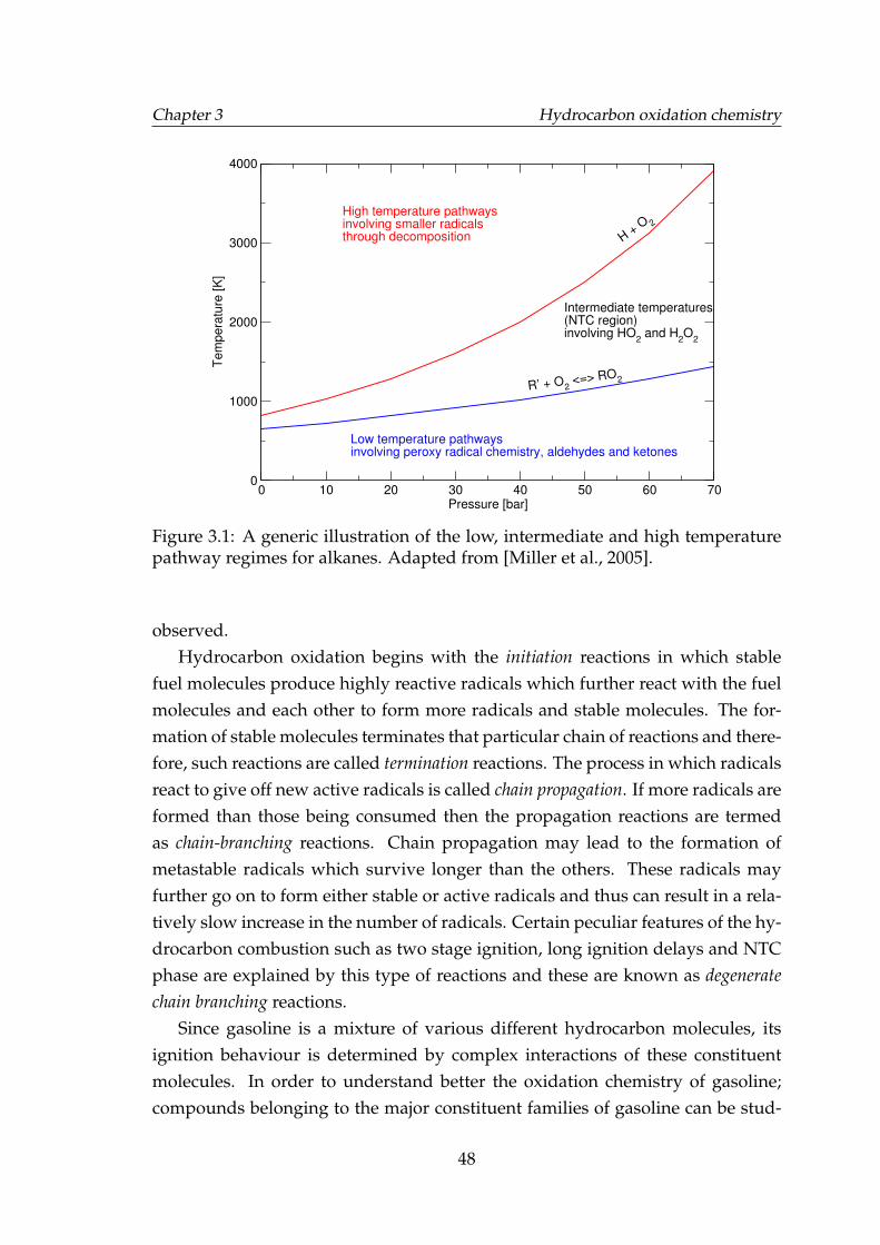
Chapter 3 Hydrocarbon oxidation chemistry
0 10 20 30 40 50 60 70Pressure [bar]
0
1000
2000
3000
4000
Tem
pera
ture
[K
]
Low temperature pathwaysinvolving peroxy radical chemistry, aldehydes and ketones
Intermediate temperatures(NTC region)involving HO
2 and H
2O
2
High temperature pathwaysinvolving smaller radicalsthrough decomposition H +
O 2
R’ + O2 <=> RO2
Figure 3.1: A generic illustration of the low, intermediate and high temperaturepathway regimes for alkanes. Adapted from [Miller et al., 2005].
observed.Hydrocarbon oxidation begins with the initiation reactions in which stable
fuel molecules produce highly reactive radicals which further react with the fuelmolecules and each other to form more radicals and stable molecules. The for-mation of stable molecules terminates that particular chain of reactions and there-fore, such reactions are called termination reactions. The process in which radicalsreact to give off new active radicals is called chain propagation. If more radicals areformed than those being consumed then the propagation reactions are termedas chain-branching reactions. Chain propagation may lead to the formation ofmetastable radicals which survive longer than the others. These radicals mayfurther go on to form either stable or active radicals and thus can result in a rela-tively slow increase in the number of radicals. Certain peculiar features of the hy-drocarbon combustion such as two stage ignition, long ignition delays and NTCphase are explained by this type of reactions and these are known as degeneratechain branching reactions.
Since gasoline is a mixture of various different hydrocarbon molecules, itsignition behaviour is determined by complex interactions of these constituentmolecules. In order to understand better the oxidation chemistry of gasoline;compounds belonging to the major constituent families of gasoline can be stud-
48
Chapter 3 Hydrocarbon oxidation chemistry
ied. The blends of these compounds can then be used as surrogates for gasoline.In this work some of the key established features of hydrocarbon oxidation
are presented and then the three reduced chemical kinetic schemes for gasolinesurrogates presented in Section 2.5 are studied. The objectives of this study are
• to identify the key mechanisms employed in these models to determine ifthey are in accord with the established understanding of hydrocarbon oxi-dation
• to investigate the interactions of intermediate radicals formed during theoxidation of gasoline surrogates, in particular the effect of toluene and ethanoladdition on the ignition precursors
• to investigate the reactivity exhibited by a gasoline surrogate in engine con-ditions and how they may lead to autoignition
3.2 General features of hydrocarbon oxidation
3.2.1 Low temperature oxidation
One of the main differences attributed to the low and high temperature oxida-tion pathways is the way the original carbon chain is broken down. At lowtemperatures the carbon chain is attacked by oxygen and various other activeradicals, most important of which are H, O, OH and HO2. The resulting radicalsundergo scission reactions which progressively shortens the carbon chain suchas C4 −→ C3 −→ C2 −→ C1. However, at higher temperatures the decompositionoccurs through the breakage of the weakest bonds (typically the tertiary bonds)resulting in a shortening of the carbon chain such as C4 −→ 2 C2 [Griffiths, 1995].Therefore, the differences in the carbon chain length of different alkanes haveperceptible differences in the low temperature oxidation chemistry. However,at high temperatures, alkanes of different lengths quickly breakdown to similarsmaller fragments and therefore size effects on the type of reaction pathways arenegligible.
The selectivity of the initiation reactions is dependent on the oxygen concen-tration and the temperature. Consider the following two possibilities of initiationreactions:
RH + O2 −→ R· + HO2 (3.1)
49
Chapter 3 Hydrocarbon oxidation chemistry
and
RH −→ R1 + R2 (3.2)
For typical alkanes, at temperatures higher than 1000 K, the reaction rate forthe H atom abstraction reaction (3.1) is 1/1000th of the decomposition initiationreaction (3.2). Therefore at temperatures higher than 1000 K, decomposition isthe more significant pathway. Whereas at temperatures below 1000 K, the pre-dominant initiation reaction is abstraction of H atom from the fuel molecule (3.1).At temperatures higher than 1400 K, decomposition is the sole initiation reaction[Griffiths and Barnard, 1995]. What follows at low temperatures from reaction(3.1) is the different ways in which its products react with its original reactants.One of the most important of these reactions is the alkyl/alkylperoxy radicalequilibrium,
R· + O2 ←→ RO2 (3.3)
The direction of reaction (3.3) has important implications on the reactions tofollow. The activation energy for the forward reaction is negligible therefore atlow temperatures more and more alkylperoxy radicals (RO2) are formed. Theactivation energy for the reverse reaction is considerable, about 30 kcal/mole foralkanes, therefore, the reverse reaction becomes dominant at high temperatures.This shift in equilibrium can be regarded as the transition from the low to in-termediate temperature range. In addition to this, a temperature increase to thebenefit of olefin formation through reaction (3.11) causes a reduction of the globalreaction rate. This results in the manifestation of the NTC behaviour typical ofmost alkanes.
After the H atom abstraction reactions, the key radicals present in the systemare R·, HO2, OH and RO2. HO2 is inactive at low temperatures and therefore con-tributes little to the chain branching. From common initiation and initial propa-gation reactions, three types of degenerate branching involving alkyl peroxy mayensue [Sokolik, 1960]. At temperature less than 650 K, the chain is mainly propa-gated through a radical attack on the fuel molecules such as:
RO2 + RH −→ R· + ROOH (3.4)
However, as the temperature increases the role of acyl hydroperoxides (see re-action 3.10) increases and finally, pathways involving formaldehyde become sig-
50
Chapter 3 Hydrocarbon oxidation chemistry
nificant. These pathways are given as follows.
RO2 −→ R·CH2CH2OO −→ R·O + CH3CHO (3.5)
RO2 −→ R”CH2O· −→ R” + CH2O (3.6)
Reactions such as (3.7) which cause the build-up of alkyl hydroperoxide rad-icals are crucial to the early stages of heat release as the weak O−O bond easilybreaks resulting in the formation of two active radicals:
ROOH −→ RO + OH (3.7)
The sudden accumulation of OH radicals results in further oxidation of thesmaller fuel fragments and partially oxidized species through exothermic reac-tions signifying a first stage mild ignition. Sokolik [1960] cites Semenov on the as-sertion that decomposition of a peroxide radical can only occur once it has under-gone internal isomerisation. This isomerisation of RO2 radicals occurs throughthe abstraction of an internal H atom from a location for which the ring-strain en-ergy and the energy for H atom abstraction is the lowest [Westbrook et al., 1991].Such a reaction can be depicted as:
RO2 −→ QOOH (3.8)
The hydroperoxyalkyl radicals (QOOH) contain a vacant bond on one of thecarbon atoms as well as the weak O−O bond as a result of which QOOH has astrong potential for undergoing four different chain branching reactions depend-ing on the temperature. Its dissociation in low and intermediate temperatureregime forms another important pathway as it produces smaller olefins and oxy-genated species such as aldehydes. Aldehydes undergo oxidation much quickerdue to the weak aldehydic C−H bond. They also have the potential to carry onchain branching and produce ROOH radicals as following; [Kolaitis and Founti,2010].
RCHO/CH2O + RO2 −→ RC·O/CHO + ROOH (3.9)
Reaction (3.9) not only contributes to the ROOH chain branching route butforms acyl radicals (RC·O), upon further oxidation of which, acyl hydroperoxyradicals, (RCO(OO·)), are formed. These radicals are more stable than alkylper-
51
Chapter 3 Hydrocarbon oxidation chemistry
oxy radicals and therefore may become important as the rate determining path-way [Koert et al., 1994]. An H atom abstraction as shown in the following reac-tion, produces acyl hydroperoxide or peracid.
RCO(OO·) + RH −→ RCO(OOH) + R· (3.10)
Koert et al. [1994] reports that although the formation and decomposition ofacyl hydroperoxide provides a low temperature pathway, it is generally regardedunimportant, possibly because acyl hydroperxide is formed through addition ofmolecular oxygen to an acyl radical, this oxygen is only abundantly availablefor fuel lean conditions and since the reactions has a high activation energy, thispathway is only important for fuel lean and high temperature conditions.
Further addition of oxygen to QOOH can also occur forming hydroperox-yalkylperoxy radicals (O2QOOH). This pathway contributes substantially to theradical pool as O2QOOH isomerises and subsequently dissociates to form keto-hydroperoxy (OQ
′OOH) and OH radicals. Further decomposition results in dike-
tone (OQ′O·) as well as OH. At relatively higher temperatures QOOH may form
through different reactions: cyclic ethers, ketones, HO2 and OH [Kolaitis andFounti, 2010].
This pathway, the isomerisation of ROO, followed by double O2 addition,has been found to be crucial in producing the NTC phase observed in alkanesand particularly the straight chained alkanes in which case the isomerisation isfavoured for reasons described in later sections. Due to this significance of theso-called peroxy radical isomerisation and decomposition (PRID) pathway, it iscentral to almost all of the PRF mechanisms. Further details on this pathway andits reaction rate parameters can be found in [Curran et al., 1998a].
As the temperature increases, the reversibility of the reaction (3.3) starts toplay its key role. The decomposition of RO2 causes a scarcity of this radical andthis in turn starves the formation of peroxide radicals. This process intensifies asthe temperature increases and more and more RO2 radicals vanish. This slow-ing down of the degenerate chain branching gives way to the non-branching re-actions which cause a decrease in the global reaction rate. As the temperatureincreases beyond the low/intermediate temperature regime, the H atom abstrac-tion reaction is not the only initiation channel. The fuel molecules undergo py-rolytic decomposition and form molecules of smaller molecular weights, includ-ing alkanes and olefins. But this is not the only source of smaller fuel molecules.From the reverse of reaction (3.3), more and more R· radicals are available to in-
52
Chapter 3 Hydrocarbon oxidation chemistry
teract with oxygen for further H atom abstraction,
R· + O2 −→ olefin + HO2 (3.11)
also, HO2 radicals are active at high temperatures in reactions such as:
RH + HO2 −→ R· + HOOH (3.12)
These alternate reactions start to compensate for the NTC phase reduction ofRO2 radicals. HO2 radicals formed in reaction (3.11) establish a H2O2 formationchannel through reaction (3.12). At higher temperatures H2O2 is unstable and fur-ther decomposes to form two OH radicals. At intermediate to high temperaturesHO2 and H2O2 functionally replace RO2 and ROOH.
3.2.2 High temperature oxidation
At high temperatures, the chain initiation reactions are predominantly the de-composition reactions in addition to the H atom abstraction reactions. Hydrocar-bon fragments thus formed are short lived and undergo α or β scission, or poly-merisation. β scission is thermodynamically favoured over α scission and it isthe dominant reaction. In β scission reactions, the bond at a distance of two fromthe free radical breaks forming an ethene. Curran et al. [1998a] classified elemen-tary reactions for n-heptane and iso-octane into 25 major classes encompassingthe whole low to high temperature regimes. They demonstrated that high tem-perature oxidation can be simulated by means of 9 classes of reactions. Thosereaction classes are not discussed here in detail, however, it is summarised thatthe decomposition of not only fuel molecules but the alkyl, alkenyl and olefins isa major branching mechanism. Internal H atom isomerisation carries on at hightemperatures. Other smaller oxygenated species such as CH2O and CO alongwith olefins and smaller alkanes take over as the main participants of the subse-quent oxidation reactions. H atom and CO oxidation is therefore central to anychemical kinetic mechanism. Participation of HO2 radicals is increased due totheir higher reactivity at these temperatures.
53
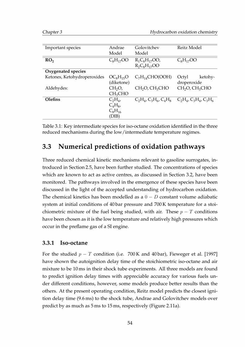
Chapter 3 Hydrocarbon oxidation chemistry
Important species AndraeModel
GolovitchevModel
Reitz Model
RO2 C8H17OO R1C8H17OO,R2C8H17OO
C8H17OO
Oxygenated speciesKetones, Ketohydroperoxides OC8H15O
(diketone)C7H14CHO(OOH) Octyl ketohy-
droperoxideAldehydes: CH2O,
CH3CHOCH2O, CH3CHO CH2O, CH3CHO
Olefins C2H4,C4H8,C8H16(DIB)
C2H4, C3H6, C4H8 C2H4, C3H4, C3H6
Table 3.1: Key intermediate species for iso-octane oxidation identified in the threereduced mechanisms during the low/intermediate temperature regimes.
3.3 Numerical predictions of oxidation pathways
Three reduced chemical kinetic mechanisms relevant to gasoline surrogates, in-troduced in Section 2.5, have been further studied. The concentrations of specieswhich are known to act as active centres, as discussed in Section 3.2, have beenmonitored. The pathways involved in the emergence of these species have beendiscussed in the light of the accepted understanding of hydrocarbon oxidation.The chemical kinetics has been modelled as a 0 − D constant volume adiabaticsystem at initial conditions of 40 bar pressure and 700 K temperature for a stoi-chiometric mixture of the fuel being studied, with air. These p − T conditionshave been chosen as it is the low temperature and relatively high pressures whichoccur in the preflame gas of a SI engine.
3.3.1 Iso-octane
For the studied p − T condition (i.e. 700 K and 40 bar), Fieweger et al. [1997]have shown the autoignition delay time of the stoichiometric iso-octane and airmixture to be 10 ms in their shock tube experiments. All three models are foundto predict ignition delay times with appreciable accuracy for various fuels un-der different conditions, however, some models produce better results than theothers. At the present operating condition, Reitz model predicts the closest igni-tion delay time (9.6 ms) to the shock tube, Andrae and Golovitchev models overpredict by as much as 5 ms to 15 ms, respectively (Figure 2.11a).
54
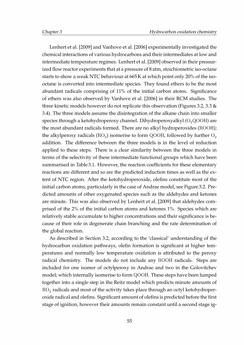
Chapter 3 Hydrocarbon oxidation chemistry
Lenhert et al. [2009] and Vanhove et al. [2006] experimentally investigated thechemical interactions of various hydrocarbons and their intermediates at low andintermediate temperature regimes. Lenhert et al. [2009] observed in their pressur-ized flow reactor experiments that at a pressure of 8 atm, stoichiometric iso-octanestarts to show a weak NTC behaviour at 665 K at which point only 20% of the iso-octane is converted into intermediate species. They found ethers to be the mostabundant radicals comprising of 11% of the initial carbon atoms. Significanceof ethers was also observed by Vanhove et al. [2006] in their RCM studies. Thethree kinetic models however do not replicate this observation (Figures 3.2, 3.3 &3.4). The three models assume the disintegration of the alkane chain into smallerspecies through a ketohydroperoxy channel. Dihydroperoxyalkyl (O2QOOH) arethe most abundant radicals formed. There are no alkyl hydroperoxides (ROOH);the alkylperoxy radicals (RO2) isomerise to form QOOH, followed by further O2
addition. The difference between the three models is in the level of reductionapplied to these steps. There is a clear similarity between the three models interms of the selectivity of these intermediate functional groups which have beensummarised in Table 3.1. However, the reaction coefficients for these elementaryreactions are different and so are the predicted induction times as well as the ex-tent of NTC region. After the ketohydroperoxide, olefins constitute most of theinitial carbon atoms, particularly in the case of Andrae model, see Figure 3.2. Pre-dicted amounts of other oxygenated species such as the aldehydes and ketonesare minute. This was also observed by Lenhert et al. [2009] that aldehydes com-prised of the 2% of the initial carbon atoms and ketones 1%. Species which arerelatively stable accumulate to higher concentrations and their significance is be-cause of their role in degenerate chain branching and the rate determination ofthe global reaction.
As described in Section 3.2, according to the ‘classical’ understanding of thehydrocarbon oxidation pathways, olefin formation is significant at higher tem-peratures and normally low temperature oxidation is attributed to the peroxyradical chemistry. The models do not include any ROOH radicals. Steps areincluded for one isomer of octylperoxy in Andrae and two in the Golovitchevmodel; which internally isomerise to form QOOH. These steps have been lumpedtogether into a single step in the Reitz model which predicts minute amounts ofRO2 radicals and most of the activity takes place through an octyl ketohydroper-oxide radical and olefins. Significant amount of olefins is predicted before the firststage of ignition, however their amounts remain constant until a second stage ig-
55
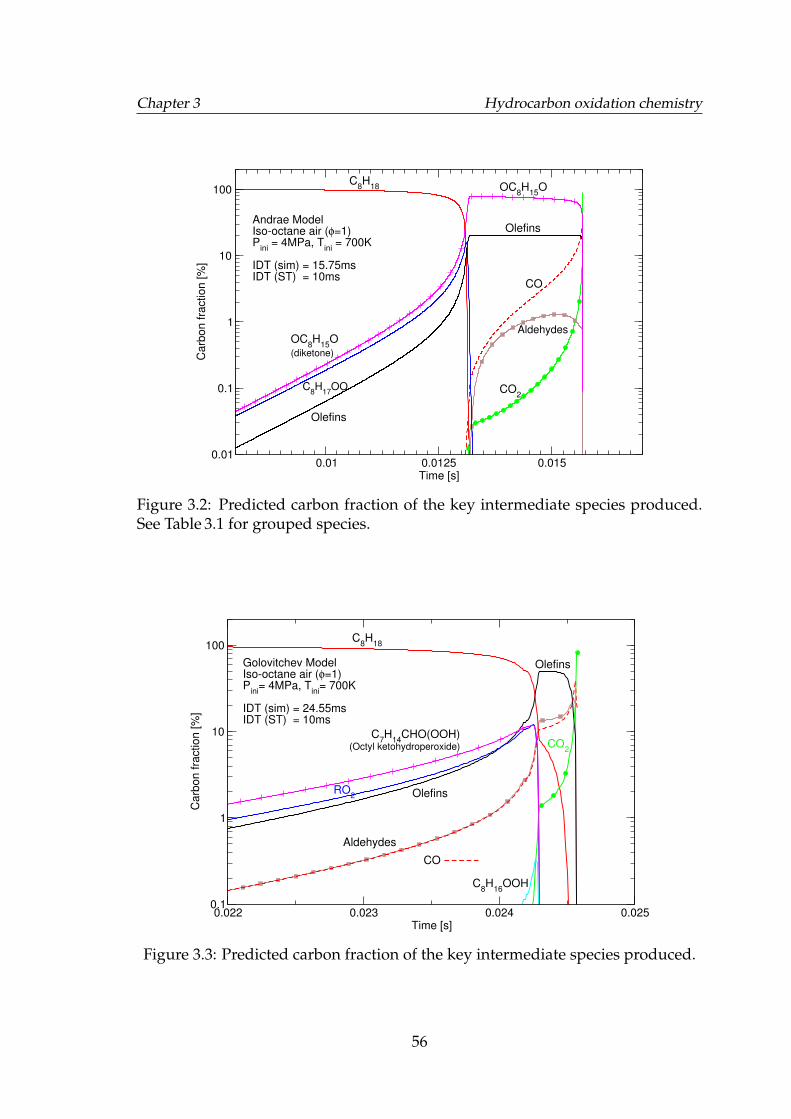
Chapter 3 Hydrocarbon oxidation chemistry
0.01 0.0125 0.015Time [s]
0.01
0.1
1
10
100C
arb
on fra
ction [%
]
C8H
18 OC8H
15O
Olefins
CO
CO2
Aldehydes
C8H
17OO
Olefins
OC8H
15O
Andrae ModelIso-octane air (φ=1)P
ini = 4MPa, T
ini = 700K
IDT (sim) = 15.75msIDT (ST) = 10ms
(diketone)
Figure 3.2: Predicted carbon fraction of the key intermediate species produced.See Table 3.1 for grouped species.
0.022 0.023 0.024 0.025Time [s]
0.1
1
10
100
Carb
on fra
ction [%
]
C8H
18
Olefins
Aldehydes
CO
CO2
C7H
14CHO(OOH)
OlefinsRO2
C8H
16OOH
Golovitchev ModelIso-octane air (φ=1)P
ini= 4MPa, T
ini= 700K
IDT (sim) = 24.55msIDT (ST) = 10ms
(Octyl ketohydroperoxide)
Figure 3.3: Predicted carbon fraction of the key intermediate species produced.
56
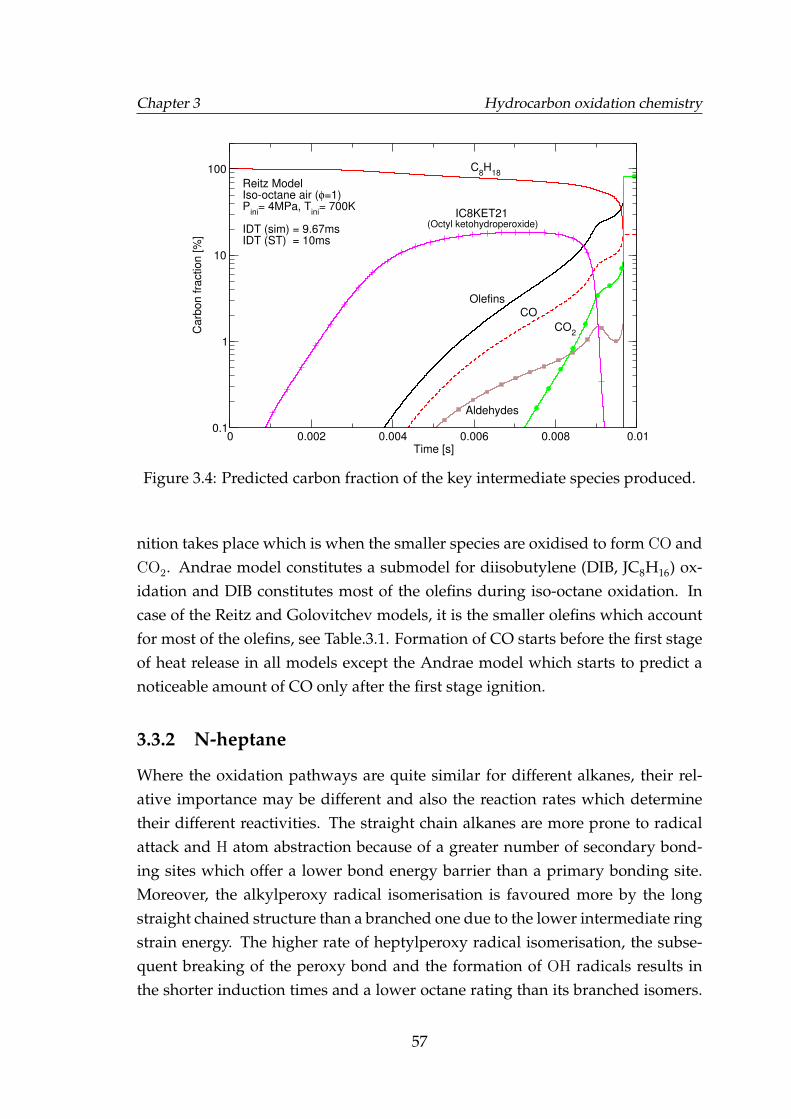
Chapter 3 Hydrocarbon oxidation chemistry
0 0.002 0.004 0.006 0.008 0.01Time [s]
0.1
1
10
100
Carb
on fra
ction [%
]
(Octyl ketohydroperoxide)
C8H
18
Olefins
Aldehydes
CO2
CO
Reitz ModelIso-octane air (φ=1)P
ini= 4MPa, T
ini= 700K
IDT (sim) = 9.67msIDT (ST) = 10ms
IC8KET21
Figure 3.4: Predicted carbon fraction of the key intermediate species produced.
nition takes place which is when the smaller species are oxidised to form CO andCO2. Andrae model constitutes a submodel for diisobutylene (DIB, JC8H16) ox-idation and DIB constitutes most of the olefins during iso-octane oxidation. Incase of the Reitz and Golovitchev models, it is the smaller olefins which accountfor most of the olefins, see Table.3.1. Formation of CO starts before the first stageof heat release in all models except the Andrae model which starts to predict anoticeable amount of CO only after the first stage ignition.
3.3.2 N-heptane
Where the oxidation pathways are quite similar for different alkanes, their rel-ative importance may be different and also the reaction rates which determinetheir different reactivities. The straight chain alkanes are more prone to radicalattack and H atom abstraction because of a greater number of secondary bond-ing sites which offer a lower bond energy barrier than a primary bonding site.Moreover, the alkylperoxy radical isomerisation is favoured more by the longstraight chained structure than a branched one due to the lower intermediate ringstrain energy. The higher rate of heptylperoxy radical isomerisation, the subse-quent breaking of the peroxy bond and the formation of OH radicals results inthe shorter induction times and a lower octane rating than its branched isomers.
57
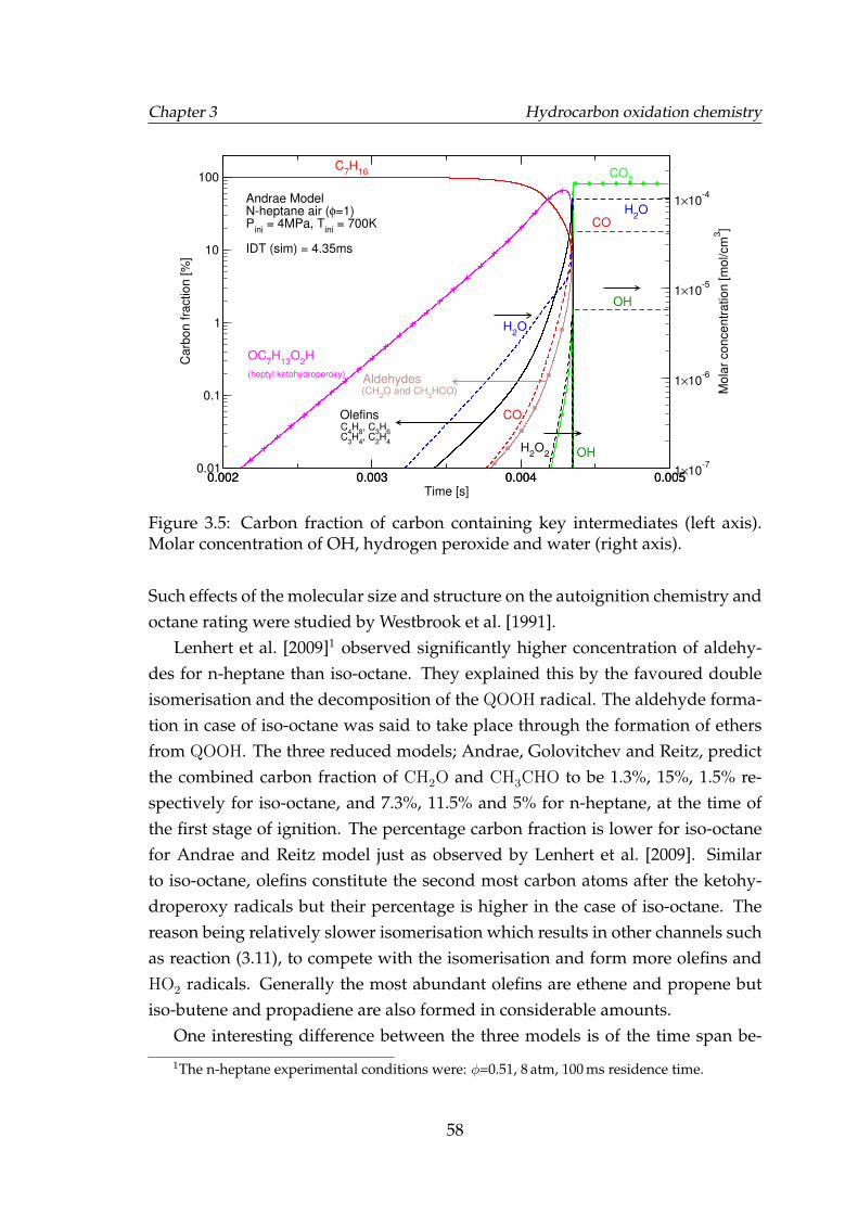
Chapter 3 Hydrocarbon oxidation chemistry
0.002 0.003 0.004 0.005Time [s]
0.01
0.1
1
10
100C
arb
on fra
ction [%
]
0.002 0.003 0.004 0.0051×10
-7
1×10⁻⁶
1×10⁻⁵
1×10⁻⁴
Mola
r concentr
ation [m
ol/cm
3]
C7H
16
OC7H
13O
2H
(heptyl ketohydroperoxy)
CO
CO2
H2O
OlefinsC
4H
8, C
3H
6C
3H
4, C
2H
4
Aldehydes(CH
2O and CH
3HCO)
H2O
2
OH
OH
Andrae ModelN-heptane air (φ=1)P
ini = 4MPa, T
ini = 700K
IDT (sim) = 4.35ms
CO
H2O
Figure 3.5: Carbon fraction of carbon containing key intermediates (left axis).Molar concentration of OH, hydrogen peroxide and water (right axis).
Such effects of the molecular size and structure on the autoignition chemistry andoctane rating were studied by Westbrook et al. [1991].
Lenhert et al. [2009]1 observed significantly higher concentration of aldehy-des for n-heptane than iso-octane. They explained this by the favoured doubleisomerisation and the decomposition of the QOOH radical. The aldehyde forma-tion in case of iso-octane was said to take place through the formation of ethersfrom QOOH. The three reduced models; Andrae, Golovitchev and Reitz, predictthe combined carbon fraction of CH2O and CH3CHO to be 1.3%, 15%, 1.5% re-spectively for iso-octane, and 7.3%, 11.5% and 5% for n-heptane, at the time ofthe first stage of ignition. The percentage carbon fraction is lower for iso-octanefor Andrae and Reitz model just as observed by Lenhert et al. [2009]. Similarto iso-octane, olefins constitute the second most carbon atoms after the ketohy-droperoxy radicals but their percentage is higher in the case of iso-octane. Thereason being relatively slower isomerisation which results in other channels suchas reaction (3.11), to compete with the isomerisation and form more olefins andHO2 radicals. Generally the most abundant olefins are ethene and propene butiso-butene and propadiene are also formed in considerable amounts.
One interesting difference between the three models is of the time span be-
1The n-heptane experimental conditions were: φ=0.51, 8 atm, 100 ms residence time.
58
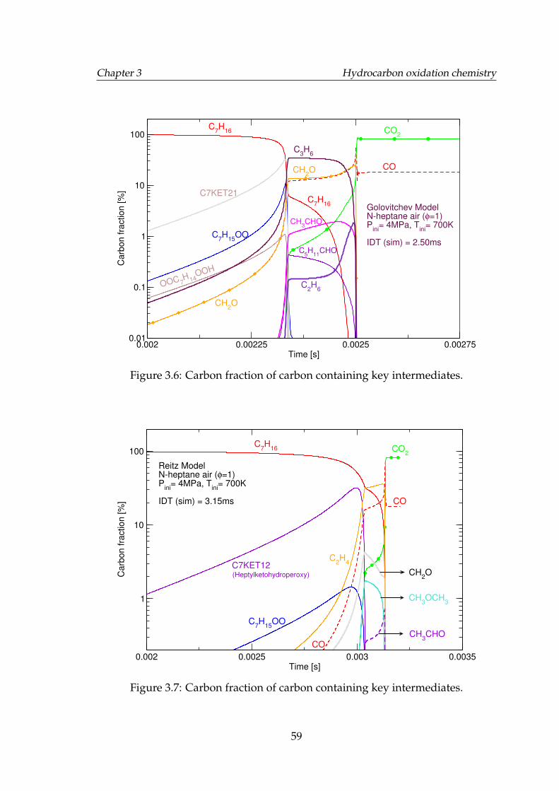
Chapter 3 Hydrocarbon oxidation chemistry
0.002 0.00225 0.0025 0.00275Time [s]
0.01
0.1
1
10
100
Ca
rbo
n f
ractio
n [
%]
C7H
16
CO
CO2
C7H
15OO
OOC 7H14
OOH
C7KET21
C5H
11CHO
CH3CHO
CH2O
C2H
6
C7H
16
CH2O
C3H
6
Golovitchev ModelN-heptane air (φ=1)P
ini= 4MPa, T
ini= 700K
IDT (sim) = 2.50ms
Figure 3.6: Carbon fraction of carbon containing key intermediates.
0.002 0.0025 0.003 0.0035Time [s]
1
10
100
Ca
rbo
n f
ractio
n [
%]
C7H
16
CO
CO2
C7H
15OO
C7KET12
CH3CHO
CH2O
C2H
4
CH3OCH
3
Reitz ModelN-heptane air (φ=1)P
ini= 4MPa, T
ini= 700K
IDT (sim) = 3.15ms
(Heptylketohydroperoxy)
CO
Figure 3.7: Carbon fraction of carbon containing key intermediates.
59
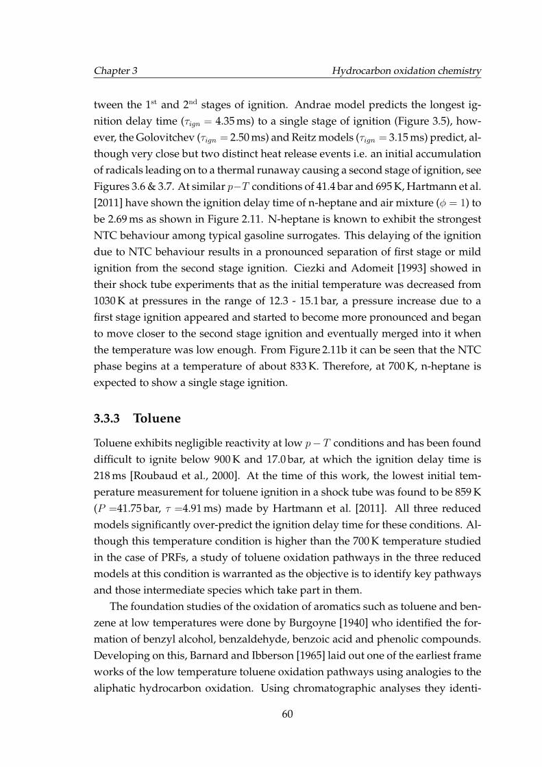
Chapter 3 Hydrocarbon oxidation chemistry
tween the 1st and 2nd stages of ignition. Andrae model predicts the longest ig-nition delay time (τign = 4.35 ms) to a single stage of ignition (Figure 3.5), how-ever, the Golovitchev (τign = 2.50 ms) and Reitz models (τign = 3.15 ms) predict, al-though very close but two distinct heat release events i.e. an initial accumulationof radicals leading on to a thermal runaway causing a second stage of ignition, seeFigures 3.6 & 3.7. At similar p−T conditions of 41.4 bar and 695 K, Hartmann et al.[2011] have shown the ignition delay time of n-heptane and air mixture (φ = 1) tobe 2.69 ms as shown in Figure 2.11. N-heptane is known to exhibit the strongestNTC behaviour among typical gasoline surrogates. This delaying of the ignitiondue to NTC behaviour results in a pronounced separation of first stage or mildignition from the second stage ignition. Ciezki and Adomeit [1993] showed intheir shock tube experiments that as the initial temperature was decreased from1030 K at pressures in the range of 12.3 - 15.1 bar, a pressure increase due to afirst stage ignition appeared and started to become more pronounced and beganto move closer to the second stage ignition and eventually merged into it whenthe temperature was low enough. From Figure 2.11b it can be seen that the NTCphase begins at a temperature of about 833 K. Therefore, at 700 K, n-heptane isexpected to show a single stage ignition.
3.3.3 Toluene
Toluene exhibits negligible reactivity at low p− T conditions and has been founddifficult to ignite below 900 K and 17.0 bar, at which the ignition delay time is218 ms [Roubaud et al., 2000]. At the time of this work, the lowest initial tem-perature measurement for toluene ignition in a shock tube was found to be 859 K(P =41.75 bar, τ =4.91 ms) made by Hartmann et al. [2011]. All three reducedmodels significantly over-predict the ignition delay time for these conditions. Al-though this temperature condition is higher than the 700 K temperature studiedin the case of PRFs, a study of toluene oxidation pathways in the three reducedmodels at this condition is warranted as the objective is to identify key pathwaysand those intermediate species which take part in them.
The foundation studies of the oxidation of aromatics such as toluene and ben-zene at low temperatures were done by Burgoyne [1940] who identified the for-mation of benzyl alcohol, benzaldehyde, benzoic acid and phenolic compounds.Developing on this, Barnard and Ibberson [1965] laid out one of the earliest frameworks of the low temperature toluene oxidation pathways using analogies to thealiphatic hydrocarbon oxidation. Using chromatographic analyses they identi-
60
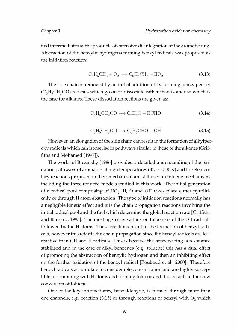
Chapter 3 Hydrocarbon oxidation chemistry
fied intermediates as the products of extensive disintegration of the aromatic ring.Abstraction of the benzylic hydrogens forming benzyl radicals was proposed asthe initiation reaction:
C6H5CH3 + O2 −→ C6H5CH2 + HO2 (3.13)
The side chain is removed by an initial addition of O2 forming benzylperoxy(C6H5CH2OO) radicals which go on to dissociate rather than isomerise which isthe case for alkanes. These dissociation rections are given as:
C6H5CH2OO −→ C6H5O + HCHO (3.14)
C6H5CH2OO −→ C6H5CHO + OH (3.15)
However, an elongation of the side chain can result in the formation of alkylper-oxy radicals which can isomerise in pathways similar to those of the alkanes (Grif-fiths and Mohamed [1997]).
The works of Brezinsky [1986] provided a detailed understanding of the oxi-dation pathways of aromatics at high temperatures (875 - 1500 K) and the elemen-tary reactions proposed in their mechanism are still used in toluene mechanismsincluding the three reduced models studied in this work. The initial generationof a radical pool comprising of HO2, H, O and OH takes place either pyroliti-cally or through H atom abstraction. The type of initiation reactions normally hasa negligible kinetic effect and it is the chain propagation reactions involving theinitial radical pool and the fuel which determine the global reaction rate [Griffithsand Barnard, 1995]. The most aggressive attack on toluene is of the OH radicalsfollowed by the H atoms. These reactions result in the formation of benzyl radi-cals, however this retards the chain propagation since the benzyl radicals are lessreactive than OH and H radicals. This is because the benzene ring is resonancestabilised and in the case of alkyl benzenes (e.g. toluene) this has a dual effectof promoting the abstraction of benzylic hydrogen and then an inhibiting effecton the further oxidation of the benzyl radical [Roubaud et al., 2000]. Thereforebenzyl radicals accumulate to considerable concentration and are highly suscep-tible to combining with H atoms and forming toluene and thus results in the slowconversion of toluene.
One of the key intermediates, benzaldehyde, is formed through more thanone channels, e.g. reaction (3.15) or through reactions of benzyl with O2 which
61
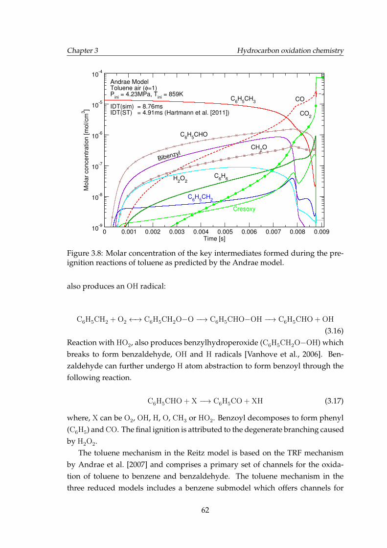
Chapter 3 Hydrocarbon oxidation chemistry
0 0.001 0.002 0.003 0.004 0.005 0.006 0.007 0.008 0.009Time [s]
10-9
10-8
10-7
10-6
10-5
10-4
Mola
r concentr
ation [m
ol/cm
3]
C6H
5CH
3
C6H
5CH
2
Cresoxy
C6H
5CHO
Bibenzyl
CO
CO2
C6H
6
CH2O
Andrae ModelToluene air (φ=1)P
ini = 4.23MPa, T
ini = 859K
IDT(sim) = 8.76msIDT(ST) = 4.91ms (Hartmann et al. [2011])
H2O
2
Figure 3.8: Molar concentration of the key intermediates formed during the pre-ignition reactions of toluene as predicted by the Andrae model.
also produces an OH radical:
C6H5CH2 + O2 ←→ C6H5CH2O−O −→ C6H5CHO−OH −→ C6H5CHO + OH
(3.16)Reaction with HO2, also produces benzylhydroperoxide (C6H5CH2O−OH) whichbreaks to form benzaldehyde, OH and H radicals [Vanhove et al., 2006]. Ben-zaldehyde can further undergo H atom abstraction to form benzoyl through thefollowing reaction.
C6H5CHO + X −→ C6H5CO + XH (3.17)
where, X can be O2, OH, H, O, CH3 or HO2. Benzoyl decomposes to form phenyl(C6H5) and CO. The final ignition is attributed to the degenerate branching causedby H2O2.
The toluene mechanism in the Reitz model is based on the TRF mechanismby Andrae et al. [2007] and comprises a primary set of channels for the oxida-tion of toluene to benzene and benzaldehyde. The toluene mechanism in thethree reduced models includes a benzene submodel which offers channels for
62
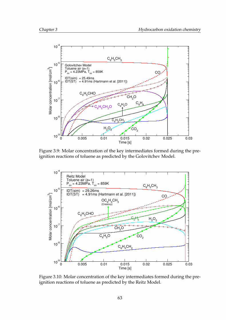
Chapter 3 Hydrocarbon oxidation chemistry
0 0.005 0.01 0.015 0.02 0.025 0.03Time [s]
10-9
10-8
10-7
10-6
10-5
10-4
Mo
lar
co
nce
ntr
atio
n [
mo
l/cm
3]
C6H
5CH
3
C6H
5CH
2
C6H
5CHO
CO
CO2
H2O
2
CH2O
C6H
5CH
2O
C6H
6
Golovitchev ModelToluene air (φ=1)P
ini = 4.23MPa, T
ini = 859K
IDT(sim) = 25.49msIDT(ST) = 4.91ms (Hartmann et al. [2011])
C6H
5O
Figure 3.9: Molar concentration of the key intermediates formed during the pre-ignition reactions of toluene as predicted by the Golovitchev Model.
0 0.005 0.01 0.015 0.02 0.025 0.03Time [s]
10-9
10-8
10-7
10-6
10-5
10-4
Mo
lar
co
nce
ntr
atio
n [
mo
l/cm
3]
C6H
5CH
3
OC6H
4CH
3(Cresoxy)
C6H
5CHO
C6H
6
C6H
5O
CO
CO2
H2O
2
CH2O
Reitz ModelToluene air (φ=1)P
ini = 4.23MPa, T
ini = 859K
IDT(sim) = 29.26msIDT(ST) = 4.91ms (Hartmann et al. [2011])
C6H
5CH
2
Figure 3.10: Molar concentration of the key intermediates formed during the pre-ignition reactions of toluene as predicted by the Reitz Model.
63
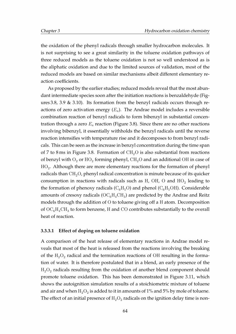
Chapter 3 Hydrocarbon oxidation chemistry
the oxidation of the phenyl radicals through smaller hydrocarbon molecules. Itis not surprising to see a great similarity in the toluene oxidation pathways ofthree reduced models as the toluene oxidation is not so well understood as isthe aliphatic oxidation and due to the limited sources of validation, most of thereduced models are based on similar mechanisms albeit different elementary re-action coefficients.
As proposed by the earlier studies; reduced models reveal that the most abun-dant intermediate species soon after the initiation reactions is benzaldehyde (Fig-ures 3.8, 3.9 & 3.10). Its formation from the benzyl radicals occurs through re-actions of zero activation energy (Ea). The Andrae model includes a reversiblecombination reaction of benzyl radicals to form bibenzyl in substantial concen-tration through a zero Ea reaction (Figure 3.8). Since there are no other reactionsinvolving bibenzyl, it essentially withholds the benzyl radicals until the reversereaction intensifies with temperature rise and it decomposes to from benzyl radi-cals. This can be seen as the increase in benzyl concentration during the time spanof 7 to 8 ms in Figure 3.8. Formation of CH2O is also substantial from reactionsof benzyl with O2 or HO2 forming phenyl, CH2O and an additional OH in case ofHO2. Although there are more elementary reactions for the formation of phenylradicals than CH2O, phenyl radical concentration is minute because of its quickerconsumption in reactions with radicals such as H, OH, O and HO2 leading tothe formation of phenoxy radicals (C6H5O) and phenol (C6H5OH). Considerableamounts of cresoxy radicals (OC6H4CH3) are predicted by the Andrae and Reitzmodels through the addition of O to toluene giving off a H atom. Decompositionof OC6H4CH3 to form benzene, H and CO contributes substantially to the overallheat of reaction.
3.3.3.1 Effect of doping on toluene oxidation
A comparison of the heat release of elementary reactions in Andrae model re-veals that most of the heat is released from the reactions involving the breakingof the H2O2 radical and the termination reactions of OH resulting in the forma-tion of water. It is therefore postulated that in a blend, an early presence of theH2O2 radicals resulting from the oxidation of another blend component shouldpromote toluene oxidation. This has been demonstrated in Figure 3.11, whichshows the autoignition simulation results of a stoichiometric mixture of tolueneand air and when H2O2 is added to it in amounts of 1% and 5% by mole of toluene.The effect of an initial presence of H2O2 radicals on the ignition delay time is non-
64
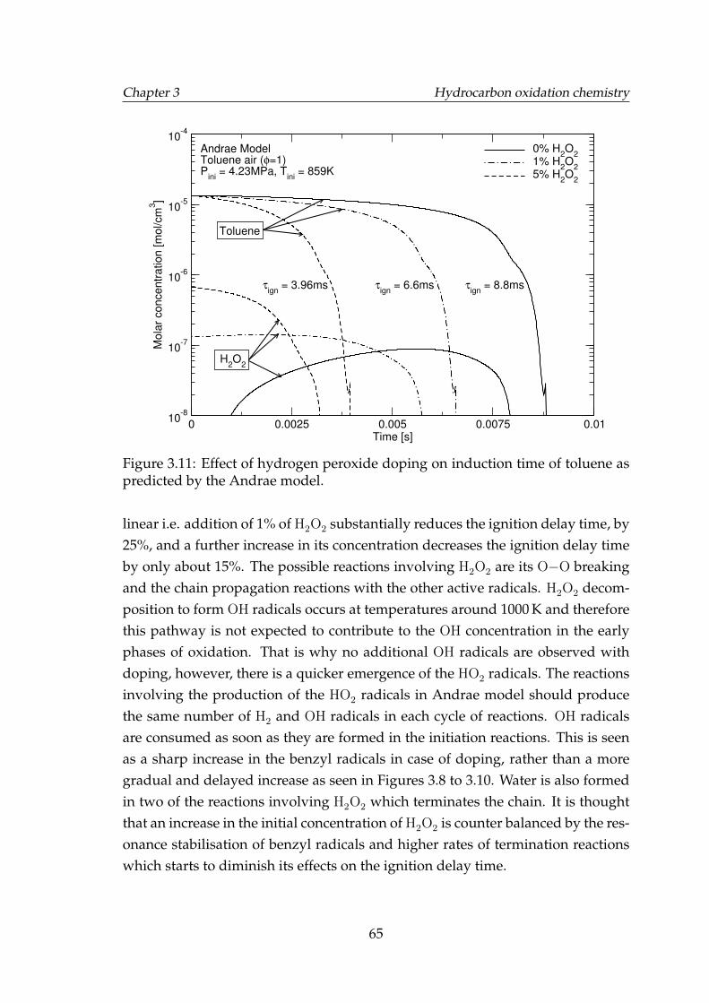
Chapter 3 Hydrocarbon oxidation chemistry
0 0.0025 0.005 0.0075 0.01Time [s]
10-8
10-7
10-6
10-5
10-4
Mola
r concentr
ation [m
ol/cm
3]
0% H2O
21% H
2O
25% H
2O
2
Andrae ModelToluene air (φ=1)P
ini = 4.23MPa, T
ini = 859K
τign
= 8.8msτign
= 6.6msτign
= 3.96ms
Toluene
H2O
2
Figure 3.11: Effect of hydrogen peroxide doping on induction time of toluene aspredicted by the Andrae model.
linear i.e. addition of 1% of H2O2 substantially reduces the ignition delay time, by25%, and a further increase in its concentration decreases the ignition delay timeby only about 15%. The possible reactions involving H2O2 are its O−O breakingand the chain propagation reactions with the other active radicals. H2O2 decom-position to form OH radicals occurs at temperatures around 1000 K and thereforethis pathway is not expected to contribute to the OH concentration in the earlyphases of oxidation. That is why no additional OH radicals are observed withdoping, however, there is a quicker emergence of the HO2 radicals. The reactionsinvolving the production of the HO2 radicals in Andrae model should producethe same number of H2 and OH radicals in each cycle of reactions. OH radicalsare consumed as soon as they are formed in the initiation reactions. This is seenas a sharp increase in the benzyl radicals in case of doping, rather than a moregradual and delayed increase as seen in Figures 3.8 to 3.10. Water is also formedin two of the reactions involving H2O2 which terminates the chain. It is thoughtthat an increase in the initial concentration of H2O2 is counter balanced by the res-onance stabilisation of benzyl radicals and higher rates of termination reactionswhich starts to diminish its effects on the ignition delay time.
65
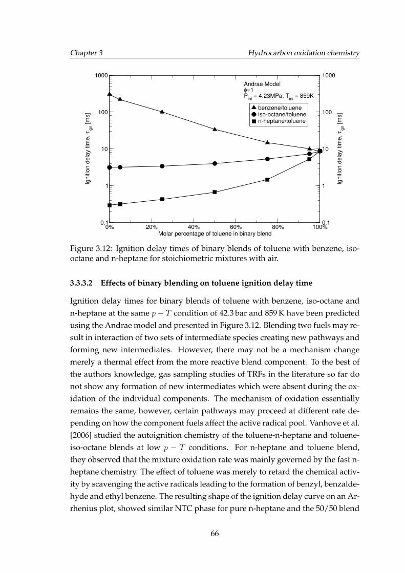
Chapter 3 Hydrocarbon oxidation chemistry
0% 20% 40% 60% 80% 100%Molar percentage of toluene in binary blend
0.1 0.1
1 1
10 10
100 100
1000 1000
Ign
itio
n d
ela
y t
ime
, τ ig
n [
ms]
Ign
itio
n d
ela
y t
ime
, τ ig
n [
ms]
benzene/tolueneiso-octane/toluenen-heptane/toluene
Andrae Modelφ=1P
ini = 4.23MPa, T
ini = 859K
Figure 3.12: Ignition delay times of binary blends of toluene with benzene, iso-octane and n-heptane for stoichiometric mixtures with air.
3.3.3.2 Effects of binary blending on toluene ignition delay time
Ignition delay times for binary blends of toluene with benzene, iso-octane andn-heptane at the same p− T condition of 42.3 bar and 859 K have been predictedusing the Andrae model and presented in Figure 3.12. Blending two fuels may re-sult in interaction of two sets of intermediate species creating new pathways andforming new intermediates. However, there may not be a mechanism changemerely a thermal effect from the more reactive blend component. To the best ofthe authors knowledge, gas sampling studies of TRFs in the literature so far donot show any formation of new intermediates which were absent during the ox-idation of the individual components. The mechanism of oxidation essentiallyremains the same, however, certain pathways may proceed at different rate de-pending on how the component fuels affect the active radical pool. Vanhove et al.[2006] studied the autoignition chemistry of the toluene-n-heptane and toluene-iso-octane blends at low p − T conditions. For n-heptane and toluene blend,they observed that the mixture oxidation rate was mainly governed by the fast n-heptane chemistry. The effect of toluene was merely to retard the chemical activ-ity by scavenging the active radicals leading to the formation of benzyl, benzalde-hyde and ethyl benzene. The resulting shape of the ignition delay curve on an Ar-rhenius plot, showed similar NTC phase for pure n-heptane and the 50/50 blend
66
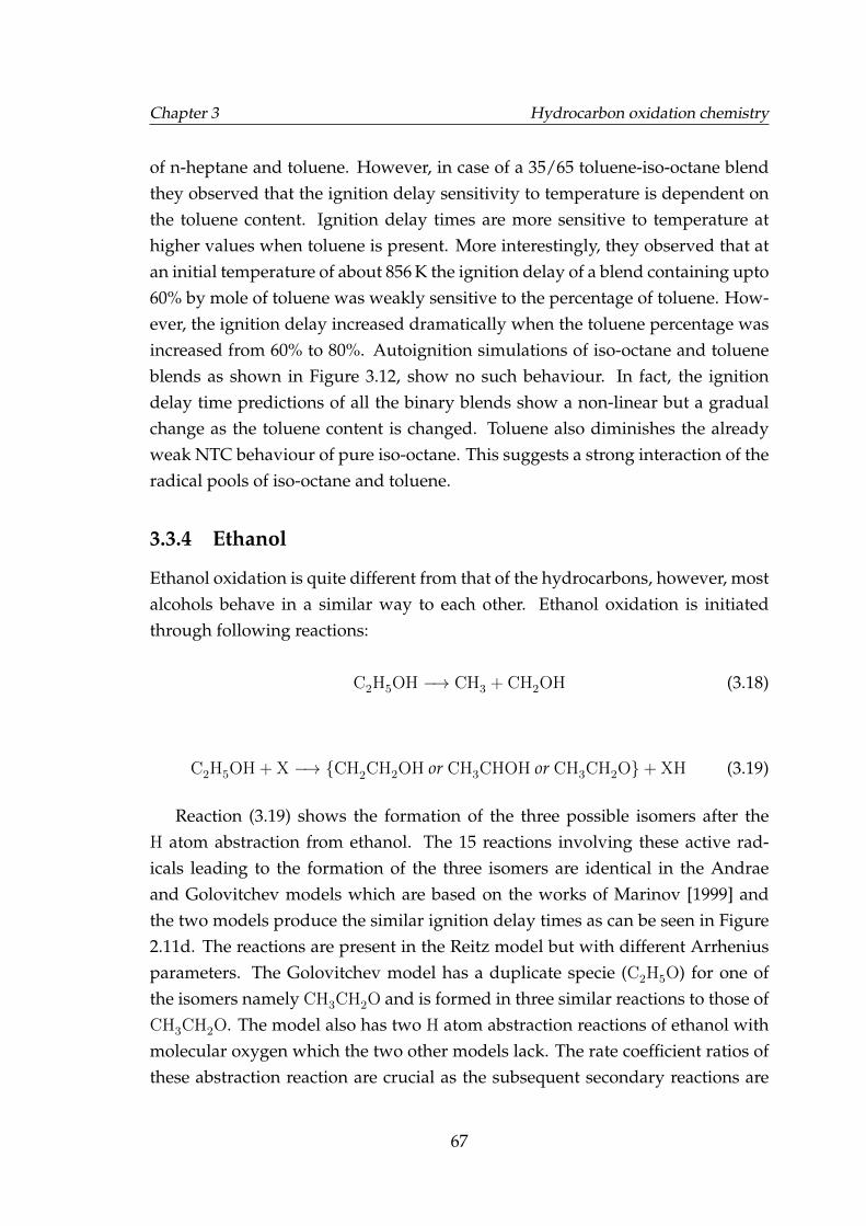
Chapter 3 Hydrocarbon oxidation chemistry
of n-heptane and toluene. However, in case of a 35/65 toluene-iso-octane blendthey observed that the ignition delay sensitivity to temperature is dependent onthe toluene content. Ignition delay times are more sensitive to temperature athigher values when toluene is present. More interestingly, they observed that atan initial temperature of about 856 K the ignition delay of a blend containing upto60% by mole of toluene was weakly sensitive to the percentage of toluene. How-ever, the ignition delay increased dramatically when the toluene percentage wasincreased from 60% to 80%. Autoignition simulations of iso-octane and tolueneblends as shown in Figure 3.12, show no such behaviour. In fact, the ignitiondelay time predictions of all the binary blends show a non-linear but a gradualchange as the toluene content is changed. Toluene also diminishes the alreadyweak NTC behaviour of pure iso-octane. This suggests a strong interaction of theradical pools of iso-octane and toluene.
3.3.4 Ethanol
Ethanol oxidation is quite different from that of the hydrocarbons, however, mostalcohols behave in a similar way to each other. Ethanol oxidation is initiatedthrough following reactions:
C2H5OH −→ CH3 + CH2OH (3.18)
C2H5OH + X −→ {CH2CH2OH or CH3CHOH or CH3CH2O}+ XH (3.19)
Reaction (3.19) shows the formation of the three possible isomers after theH atom abstraction from ethanol. The 15 reactions involving these active rad-icals leading to the formation of the three isomers are identical in the Andraeand Golovitchev models which are based on the works of Marinov [1999] andthe two models produce the similar ignition delay times as can be seen in Figure2.11d. The reactions are present in the Reitz model but with different Arrheniusparameters. The Golovitchev model has a duplicate specie (C2H5O) for one ofthe isomers namely CH3CH2O and is formed in three similar reactions to those ofCH3CH2O. The model also has two H atom abstraction reactions of ethanol withmolecular oxygen which the two other models lack. The rate coefficient ratios ofthese abstraction reaction are crucial as the subsequent secondary reactions are
67
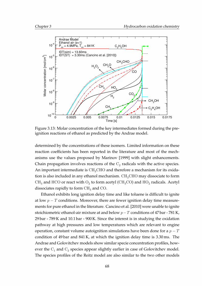
Chapter 3 Hydrocarbon oxidation chemistry
0 0.0025 0.005 0.0075 0.01 0.0125 0.015 0.0175Time [s]
10-10
10-9
10-8
10-7
10-6
10-5
10-4
Mola
r concentr
ation [m
ol/cm
3]
C2H
5OH
CH3CHO
CH2OH
2O
2
CH4
CO
HO2
H2
CH3
CO2
CH3OH
C2H
4OH
Andrae ModelEthanol air (φ=1)P
ini = 4.9MPa, T
ini = 841K
IDT(sim) = 13.60msIDT(ST) = 3.30ms (Cancino et al. [2010])
Figure 3.13: Molar concentration of the key intermediates formed during the pre-ignition reactions of ethanol as predicted by the Andrae model.
determined by the concentrations of these isomers. Limited information on thesereaction coefficients has been reported in the literature and most of the mech-anisms use the values proposed by Marinov [1999] with slight enhancements.Chain propagation involves reactions of the C2 radicals with the active species.An important intermediate is CH3CHO and therefore a mechanism for its oxida-tion is also included in any ethanol mechanism. CH3CHO may dissociate to formCH3 and HCO or react with O2 to form acetyl (CH3CO) and HO2 radicals. Acetyldissociates rapidly to form CH3 and CO.
Ethanol exhibits long ignition delay time and like toluene is difficult to igniteat low p − T conditions. Moreover, there are fewer ignition delay time measure-ments for pure ethanol in the literature. Cancino et al. [2010] were unable to ignitestoichiometric ethanol-air mixture at and below p−T conditions of 47 bar - 781 K,29 bar - 789 K and 10.1 bar - 900 K. Since the interest is in studying the oxidationpathway at high pressures and low temperatures which are relevant to engineoperation, constant volume autoignition simulations have been done for a p − Tcondition of 49 bar and 841 K, at which the ignition delay time is 3.30 ms. TheAndrae and Golovitchev models show similar specie concentration profiles, how-ever the C1 and C2 species appear slightly earlier in case of Golovitchev model.The species profiles of the Reitz model are also similar to the two other models
68
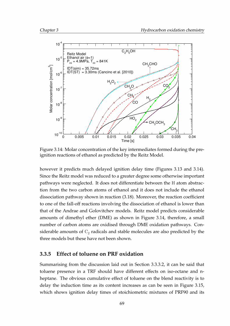
Chapter 3 Hydrocarbon oxidation chemistry
0 0.005 0.01 0.015 0.02 0.025 0.03 0.035 0.04Time [s]
10-10
10-9
10-8
10-7
10-6
10-5
10-4
Mola
r concentr
ation [m
ol/cm
3]
Reitz ModelEthanol air (φ=1)P
ini = 4.9MPa, T
ini = 841K
IDT(sim) = 35.72msIDT(ST) = 3.30ms (Cancino et al. [2010])
C2H
5OH
CH2O
CH3CHO
H2O
2
CO
CH4 H
2
HO2
CO2
CH3OCH
3
CH3
Figure 3.14: Molar concentration of the key intermediates formed during the pre-ignition reactions of ethanol as predicted by the Reitz Model.
however it predicts much delayed ignition delay time (Figures 3.13 and 3.14).Since the Reitz model was reduced to a greater degree some otherwise importantpathways were neglected. It does not differentiate between the H atom abstrac-tion from the two carbon atoms of ethanol and it does not include the ethanoldissociation pathway shown in reaction (3.18). Moreover, the reaction coefficientto one of the fall-off reactions involving the dissociation of ethanol is lower thanthat of the Andrae and Golovitchev models. Reitz model predicts considerableamounts of dimethyl ether (DME) as shown in Figure 3.14, therefore, a smallnumber of carbon atoms are oxidised through DME oxidation pathways. Con-siderable amounts of C2 radicals and stable molecules are also predicted by thethree models but these have not been shown.
3.3.5 Effect of toluene on PRF oxidation
Summarising from the discussion laid out in Section 3.3.3.2, it can be said thattoluene presence in a TRF should have different effects on iso-octane and n-heptane. The obvious cumulative effect of toluene on the blend reactivity is todelay the induction time as its content increases as can be seen in Figure 3.15,which shows ignition delay times of stoichiometric mixtures of PRF90 and its
69
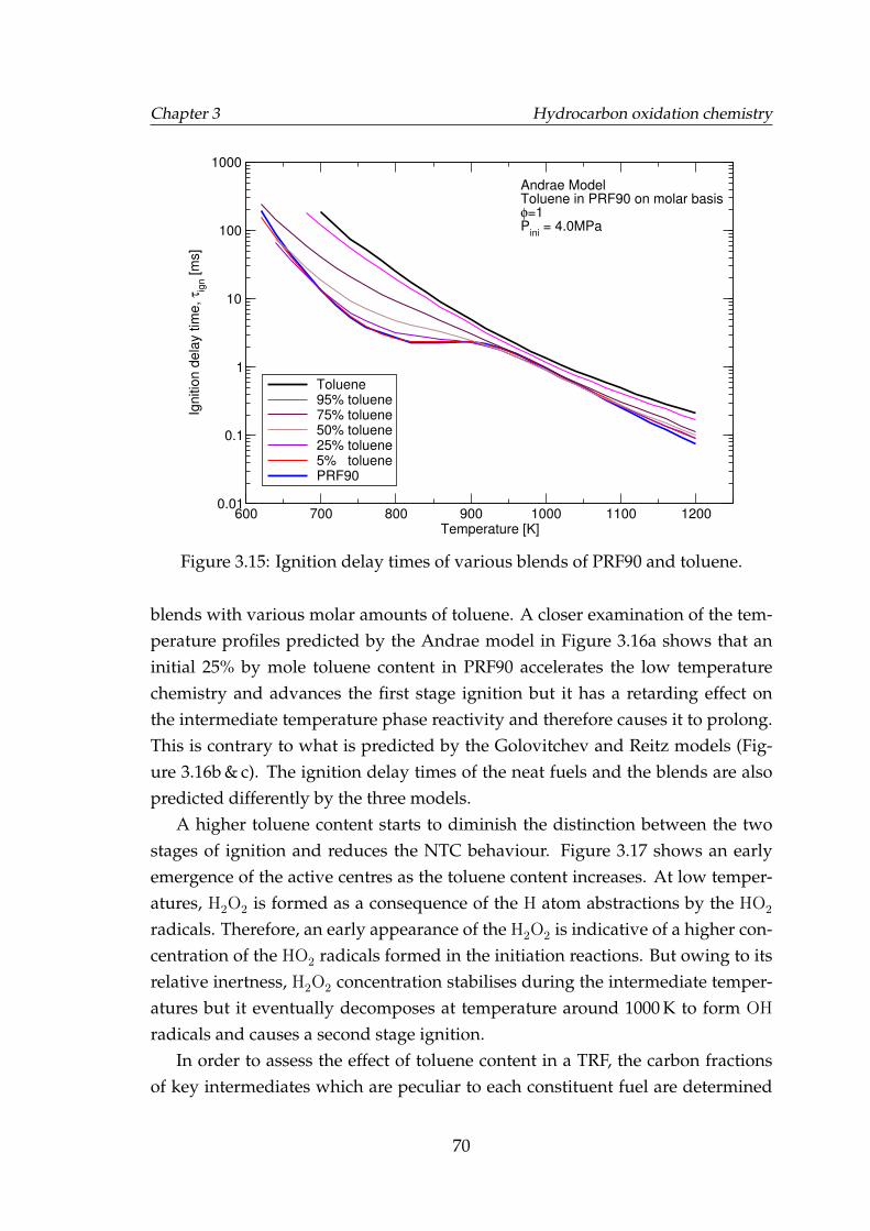
Chapter 3 Hydrocarbon oxidation chemistry
600 700 800 900 1000 1100 1200Temperature [K]
0.01
0.1
1
10
100
1000
Ign
itio
n d
ela
y t
ime
, τ ig
n [
ms]
Toluene95% toluene 75% toluene 50% toluene 25% toluene 5% toluene PRF90
Andrae ModelToluene in PRF90 on molar basisφ=1P
ini = 4.0MPa
Figure 3.15: Ignition delay times of various blends of PRF90 and toluene.
blends with various molar amounts of toluene. A closer examination of the tem-perature profiles predicted by the Andrae model in Figure 3.16a shows that aninitial 25% by mole toluene content in PRF90 accelerates the low temperaturechemistry and advances the first stage ignition but it has a retarding effect onthe intermediate temperature phase reactivity and therefore causes it to prolong.This is contrary to what is predicted by the Golovitchev and Reitz models (Fig-ure 3.16b & c). The ignition delay times of the neat fuels and the blends are alsopredicted differently by the three models.
A higher toluene content starts to diminish the distinction between the twostages of ignition and reduces the NTC behaviour. Figure 3.17 shows an earlyemergence of the active centres as the toluene content increases. At low temper-atures, H2O2 is formed as a consequence of the H atom abstractions by the HO2
radicals. Therefore, an early appearance of the H2O2 is indicative of a higher con-centration of the HO2 radicals formed in the initiation reactions. But owing to itsrelative inertness, H2O2 concentration stabilises during the intermediate temper-atures but it eventually decomposes at temperature around 1000 K to form OH
radicals and causes a second stage ignition.In order to assess the effect of toluene content in a TRF, the carbon fractions
of key intermediates which are peculiar to each constituent fuel are determined
70
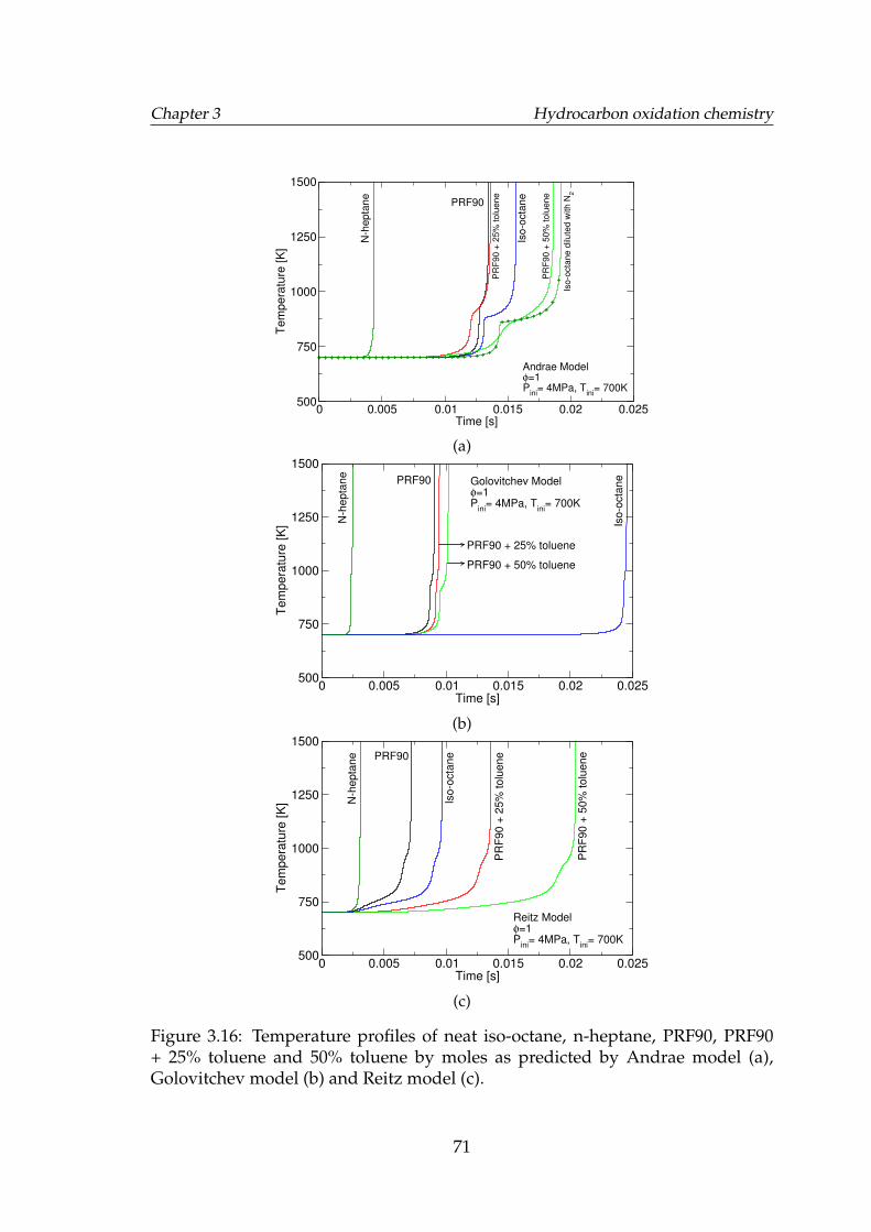
Chapter 3 Hydrocarbon oxidation chemistry
0 0.005 0.01 0.015 0.02 0.025Time [s]
500
750
1000
1250
1500
Te
mp
era
ture
[K
]
Andrae Modelφ=1P
ini= 4MPa, T
ini= 700K
N-h
epta
ne
Iso-o
cta
ne
PRF90
PR
F90 +
50%
tolu
ene
PR
F90 +
25%
tolu
ene
Iso-o
cta
ne d
ilute
d w
ith N
2
(a)
0 0.005 0.01 0.015 0.02 0.025Time [s]
500
750
1000
1250
1500
Te
mp
era
ture
[K
]
Golovitchev Modelφ=1P
ini= 4MPa, T
ini= 700K
PRF90
Iso-o
cta
ne
N-h
epta
ne
PRF90 + 25% toluene
PRF90 + 50% toluene
(b)
0 0.005 0.01 0.015 0.02 0.025Time [s]
500
750
1000
1250
1500
Te
mp
era
ture
[K
]
Reitz Modelφ=1P
ini= 4MPa, T
ini= 700K
PRF90
Iso-o
cta
ne
N-h
epta
ne
PR
F90 +
25%
tolu
ene
PR
F90 +
50%
tolu
ene
(c)
Figure 3.16: Temperature profiles of neat iso-octane, n-heptane, PRF90, PRF90+ 25% toluene and 50% toluene by moles as predicted by Andrae model (a),Golovitchev model (b) and Reitz model (c).
71
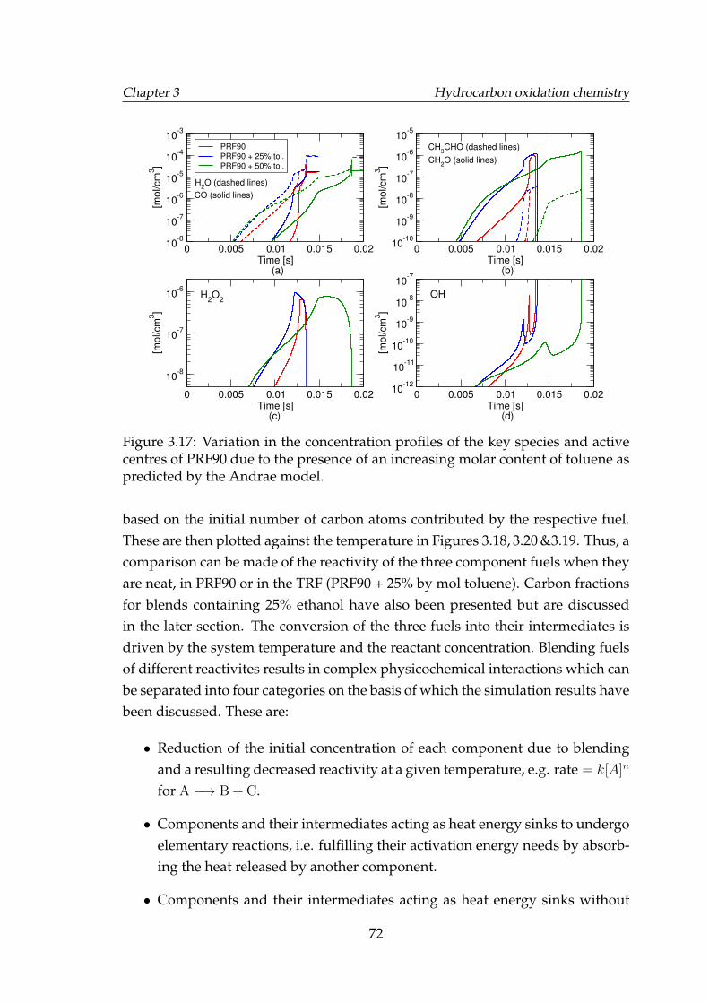
Chapter 3 Hydrocarbon oxidation chemistry
0 0.005 0.01 0.015 0.02Time [s] (a)
10-8
10-7
10-6
10-5
10-4
10-3
[mol/cm
3]
PRF90
PRF90 + 25% tol.
PRF90 + 50% tol.
0 0.005 0.01 0.015 0.02Time [s] (b)
10-10
10-9
10-8
10-7
10-6
10-5
[mol/cm
3]
0 0.005 0.01 0.015 0.02Time [s] (c)
10-8
10-7
10-6
[mol/cm
3]
0 0.005 0.01 0.015 0.02Time [s] (d)
10-12
10-11
10-10
10-9
10-8
10-7
[mol/cm
3]
H2O
2
CH2O (solid lines)
CH3CHO (dashed lines)
OH
CO (solid lines)
H2O (dashed lines)
Figure 3.17: Variation in the concentration profiles of the key species and activecentres of PRF90 due to the presence of an increasing molar content of toluene aspredicted by the Andrae model.
based on the initial number of carbon atoms contributed by the respective fuel.These are then plotted against the temperature in Figures 3.18, 3.20 &3.19. Thus, acomparison can be made of the reactivity of the three component fuels when theyare neat, in PRF90 or in the TRF (PRF90 + 25% by mol toluene). Carbon fractionsfor blends containing 25% ethanol have also been presented but are discussedin the later section. The conversion of the three fuels into their intermediates isdriven by the system temperature and the reactant concentration. Blending fuelsof different reactivites results in complex physicochemical interactions which canbe separated into four categories on the basis of which the simulation results havebeen discussed. These are:
• Reduction of the initial concentration of each component due to blendingand a resulting decreased reactivity at a given temperature, e.g. rate = k[A]n
for A −→ B + C.
• Components and their intermediates acting as heat energy sinks to undergoelementary reactions, i.e. fulfilling their activation energy needs by absorb-ing the heat released by another component.
• Components and their intermediates acting as heat energy sinks without
72
Chapter 3 Hydrocarbon oxidation chemistry
undergoing any reactions. This is the role played by a diluent such as N2.
• Chemical interaction of blend components and their intermediates openingup new pathways and also activating or deactivating the radical pool.
The almost instantaneous increase in the temperature in Figures 3.16 marksthe moment of ignition which is also coincident with the complete conversionof the fuel molecules into intermediate species. Therefore, the advanced ignitionfor PRF90 and PRF90 + 25% toluene from that of neat iso-octane is synonymousto an earlier conversion of iso-octane (not shown here), however, the percentageof iso-octane when blended is correspondingly higher than neat iso-octane at agiven temperature, see Figure 3.18a. This means that although iso-octane con-verts quicker in time but its reactivity is reduced at any given temperature. Thereason for this may seem to be a decrease in the concentration of iso-octane due toblending and its faster conversion is simply brought about due to an earlier heatrelease from the oxidation of more reactive component of the blend i.e. n-heptanein this case. However, the reduced reaction rate due to reduced concentration isnot the sole consequence of blending. Interactions between the blend compo-nents also occur and may affect the reactivity of individual components. E.g. inAndrae model, heptyl radicals abstract H atoms from iso-octane and toluene toform n-heptane (thus explaining the decrease in n-heptane’s reactivity) but theseH atom abstractions from iso-octane are not enough to compensate for its reducedreactivity. The effect of reduced concentration of iso-octane due to blending canbe separated from the presence of other reactive components by replacing themwith N2. Simulation has been done for a stoichiometric iso-octane air mixture di-luted with N2 such that the total number of moles are the same as in the case ofPRF90 + 25% by mole toluene. Therefore, the same initial concentration of iso-octane is achieved as in the case of PRF90 + 25% toluene. The resulting carbonfraction of iso-octane is presented in Figure 3.18a and its temperature profile ispresented in Figure 3.16a. It can be seen that although due to dilution the ignitionis further delayed but the conversion rate of iso-octane at any given temperatureis the highest when it is diluted, even more so than the stoichiometric mixture ofneat iso-octane and air. This indicates that the reduced reactivity of iso-octane inblended form is not caused by a reduction in its concentration but mainly due toa scarcity of the active radicals because of a higher demand for them from var-ious fuel fragments resulting in lower reaction rates. These fuel fragments thusformed scavenge the active radicals bringing the whole system to a bottle neck
73
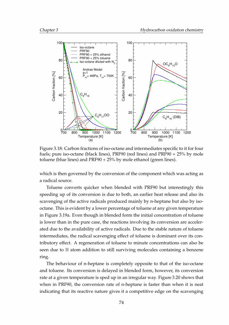
Chapter 3 Hydrocarbon oxidation chemistry
700 800 900 1000 1100 1200Temperature [K] (a)
0
20
40
60
80
100
Carb
on fra
ction [%
]
Iso-octanePRF90PRF90 + 25% ethanolPRF90 + 25% tolueneIso-octane diluted with N
2
700 800 900 1000 1100 1200Temperature [K] (b)
0
20
40
60
80
100
Carb
on fra
ction [%
]
Andrae Modelφ=1P
ini= 4MPa, T
ini= 700K
C8H
18
C8H
17OO
OC8H
15O
C8H
16 (DIB)
Figure 3.18: Carbon fractions of iso-octane and intermediates specific to it for fourfuels; pure iso-octane (black lines), PRF90 (red lines) and PRF90 + 25% by moletoluene (blue lines) and PRF90 + 25% by mole ethanol (green lines).
which is then governed by the conversion of the component which was acting asa radical source.
Toluene converts quicker when blended with PRF90 but interestingly thisspeeding up of its conversion is due to both, an earlier heat release and also itsscavenging of the active radicals produced mainly by n-heptane but also by iso-octane. This is evident by a lower percentage of toluene at any given temperaturein Figure 3.19a. Even though in blended form the initial concentration of tolueneis lower than in the pure case, the reactions involving its conversion are acceler-ated due to the availability of active radicals. Due to the stable nature of tolueneintermediates, the radical scavenging effect of toluene is dominant over its con-tributory effect. A regeneration of toluene to minute concentrations can also beseen due to H atom addition to still surviving molecules containing a benzenering.
The behaviour of n-heptane is completely opposite to that of the iso-octaneand toluene. Its conversion is delayed in blended form, however, its conversionrate at a given temperature is sped up in an irregular way. Figure 3.20 shows thatwhen in PRF90, the conversion rate of n-heptane is faster than when it is neatindicating that its reactive nature gives it a competitive edge on the scavenging
74
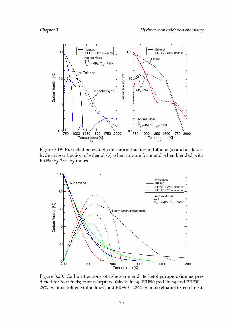
Chapter 3 Hydrocarbon oxidation chemistry
750 1000 1250 1500 1750 2000Temperature [K] (a)
0.1
1
10
100C
arb
on fra
ction [%
]ToluenePRF90 + 25% toluene
750 1000 1250 1500 1750 2000Temperature [K] (b)
0.1
1
10
100
Carb
on fra
ction [%
]
EthanolPRF90 + 25% ethanol
Toluene
Benzaldehyde
Ethanol
CH3CHO
Andrae Modelφ=1P
ini= 4MPa, T
ini= 700K
Andrae Modelφ=1P
ini= 4MPa, T
ini= 700K
Figure 3.19: Predicted benzaldehyde carbon fraction of toluene (a) and acetalde-hyde carbon fraction of ethanol (b) when in pure form and when blended withPRF90 by 25% by moles.
700 800 900 1000 1100 1200Temperature [K]
0
20
40
60
80
100
Carb
on fra
ction [%
]
N-heptane
PRF90PRF90 + 25% ethanol
PRF90 + 25% toluene
Andrae Modelφ=1P
ini= 4MPa, T
ini= 700K
N-heptane
Heptyl ketohydroperoxide
Figure 3.20: Carbon fractions of n-heptane and its ketohydroperoxide as pre-dicted for four fuels; pure n-heptane (black lines), PRF90 (red lines) and PRF90 +25% by mole toluene (blue lines) and PRF90 + 25% by mole ethanol (green lines).
75
Chapter 3 Hydrocarbon oxidation chemistry
of the active radicals produced by itself as well as iso-octane. The relationshipbetween n-heptane and iso-octane is of n-heptane acting primarily as a source ofradicals for initiation reactions and activation energy and iso-octane, primarily asource of radicals for the chain propagation of n-heptane. It appears that in a TRF,the reactivity of n-heptane is initially slowed down upto a temperature of about830 K indicating the greater radical scavenging effect of toluene. At higher tem-peratures the conversion of n-heptane is quicker possibly due to the contributionof otherwise stable components to the active radical pool. From these observa-tions, it can be hypothesised that in a TRF blend, n-heptane owing to its reactivenature acts as a source of activation energy and an initial radical pool for the lessreactive fuels which then breakdown and become a source of active radicals to bescavenged by more reactive fuel fragments of n-heptane and toluene.
3.3.6 Effect of ethanol on PRF oxidation
In order to identify the effect of ethanol presence in a PRF, constant volume adia-batic simulations have been performed for mixtures of 5%, 25% and 50% by molesethanol in PRF90 using the three reduced mechanisms. The temperature profilesfor each blend and the neat fuels show the global reactivity and also the possiblepresence of a first stage mild ignition as shown in Figure 3.21. As previously seenin the case of toluene presence in PRF90, the three mechanisms simulate the effectof ethanol addition differently. The ignition delay time predictions of the threemodels for a blend containing 40% ethanol by moles in PRF77 (Fuel-B in Fikriet al. [2008]) show that the models predict poorly at low temperatures i.e. <833 K(Figure 2.13b). At higher temperatures Andrae and Reitz models predictions areappreciably accurate. The inaccuracies at low temperatures and the lack of ex-perimental data for ethanol-PRF blends makes it difficult to state which modelpredicts the correct blending effect. Experimental ignition delay times in Fig-ure 3.22 show that neat ethanol ignites at very similar times to that of iso-octane.Measurements in [Cancino et al., 2011] also show that the ignition delay times ofa 25% ethanol and 75% iso-octane by volume blend are comparable to those ofiso-octane. This suggests that ethanol addition in iso-octane does not increase theignition delay time drastically. This is also reinforced by the RON/MON tests ofFoong et al. [2014] which show that about 30% by moles ethanol in PRF90 willbring the RON of the resulting blend to 100 i.e. equal to iso-octane. However,these observations do not lend any credence to the simulated blending effects.Some similarity is observed between the Andrae and the Reitz models in that the
76
Chapter 3 Hydrocarbon oxidation chemistry
ignition occurs for 25% and 50% by mole addition of ethanol later than iso-octaneand roughly at similar times.
Carbon fractions of iso-octane, n-heptane and ethanol during their oxidationin their pure form, in PRF90 and in a PRF90 + 25% by mole ethanol blend are alsopresented in Figures 3.18, 3.20 &3.19. The effect of ethanol presence on the reac-tivity of all three components are similar to those of toluene but more pronouncedindicating a stronger radical scavenging effect of ethanol.
3.3.7 Discussion of chemical kinetics modelling
The 0 − D ignition delay time predictions of the four major gasoline surrogatecomponents; iso-octane, n-heptane, toluene and ethanol, show an appreciablegeneral agreement with the experimental measurements. However, the modelstend to deviate from measurements at lower temperatures and during the NTCphase of the fuels. The difficulty in validation of mechanisms at low tempera-tures arises from both the chemical complexities at these regimes as well as theshortcomings of the experimental apparatuses. It has been well known that thelow/intermediate temperature chemistry is more complicated than the high tem-perature chemistry. The effects of molecular size and geometry on the pathwaysis much more pronounced at low/intermediate temperatures. Moreover, isomersof one compound may exhibit differing reaction coefficients and preference forpathways. This renders the generalisation of the chemical kinetics of one par-ticular compound for others, difficult. One of the main objectives of mechanismreduction is therefore to find the right balance between generalisation and ac-curacy. This is much more difficult to achieve in multi-component mechanismswhich comprise of pathways for the interaction of intermediate species of differ-ent fuel molecules. The reduced mechanisms studied presently, produce goodpredictions for iso-octane and n-heptane with the Reitz model having the mostaccurate PRF submodel but it is only the Andrae model which predicts well fortoluene and ethanol at high pressure (Figure 2.11). The models predict acceptableignition delay times for a TRF blend (Figure 2.13a), however, the low temperaturepredictions for an ethanol-PRF blend (Figure 2.13b) are poor.
The uncertainty of experimental measurements cannot be ignored, particu-larly at low temperatures where the ignition delay times are much longer andthe effects of heat loss and charge non-homogeneity are pronounced. Since shocktube is a wave reactor, it is more suitable for measurements at high temperatureswhen the ignition delay times are shorter. The temperature increase is achieved
77
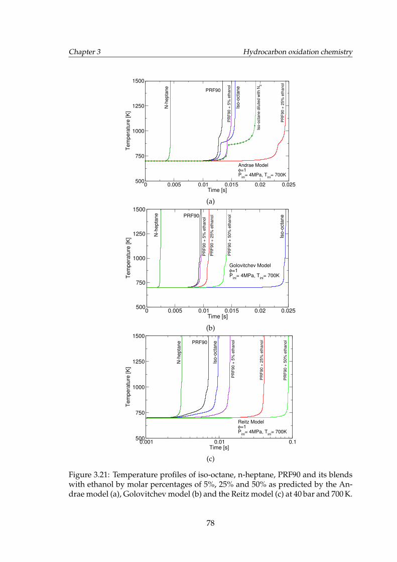
Chapter 3 Hydrocarbon oxidation chemistry
0 0.005 0.01 0.015 0.02 0.025Time [s]
500
750
1000
1250
1500
Te
mp
era
ture
[K
]
Andrae Modelφ=1P
ini= 4MPa, T
ini= 700K
N-h
epta
ne
Iso-o
cta
ne
PRF90
PR
F90 +
5%
eth
anol
PR
F90 +
25%
eth
anol
Iso-o
cta
ne d
ilute
d w
ith N
2
(a)
0 0.005 0.01 0.015 0.02 0.025Time [s]
500
750
1000
1250
1500
Te
mp
era
ture
[K
]
Golovitchev Modelφ=1P
ini= 4MPa, T
ini= 700K
PRF90
Iso-o
cta
ne
N-h
epta
ne
PR
F9
0 +
25
% e
tha
no
l
PR
F9
0 +
50
% e
tha
no
l
PR
F9
0 +
5%
eth
an
ol
(b)
0.001 0.01 0.1Time [s]
500
750
1000
1250
1500
Te
mp
era
ture
[K
]
Iso
-octa
ne
N-h
ep
tan
e PRF90
PR
F9
0 +
5%
eth
an
ol
PR
F9
0 +
25
% e
tha
no
l
PR
F9
0 +
50
% e
tha
no
l
Reitz Modelφ=1P
ini= 4MPa, T
ini= 700K
(c)
Figure 3.21: Temperature profiles of iso-octane, n-heptane, PRF90 and its blendswith ethanol by molar percentages of 5%, 25% and 50% as predicted by the An-drae model (a), Golovitchev model (b) and the Reitz model (c) at 40 bar and 700 K.
78
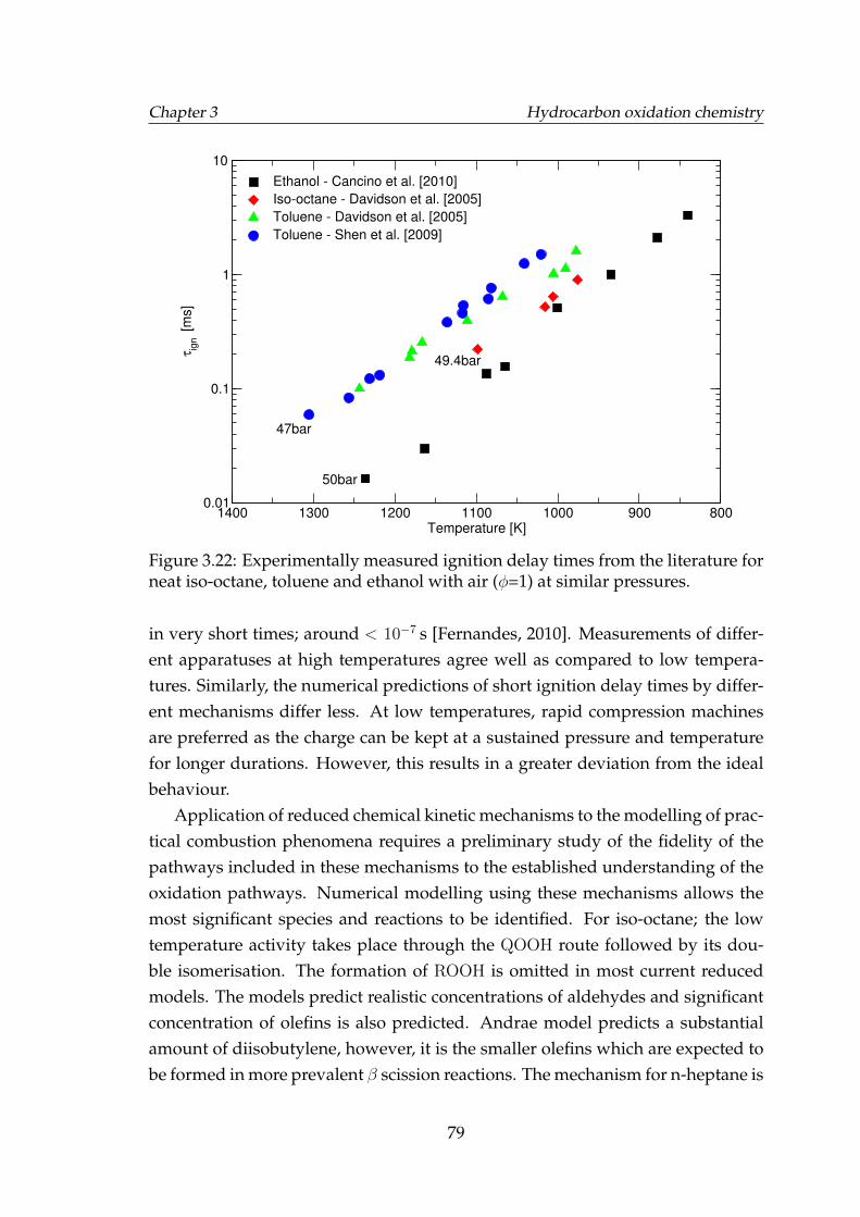
Chapter 3 Hydrocarbon oxidation chemistry
80090010001100120013001400Temperature [K]
0.01
0.1
1
10
τig
n [
ms]
Ethanol - Cancino et al. [2010]
Iso-octane - Davidson et al. [2005]
Toluene - Davidson et al. [2005]
Toluene - Shen et al. [2009]
47bar
50bar
49.4bar
Figure 3.22: Experimentally measured ignition delay times from the literature forneat iso-octane, toluene and ethanol with air (φ=1) at similar pressures.
in very short times; around < 10−7 s [Fernandes, 2010]. Measurements of differ-ent apparatuses at high temperatures agree well as compared to low tempera-tures. Similarly, the numerical predictions of short ignition delay times by differ-ent mechanisms differ less. At low temperatures, rapid compression machinesare preferred as the charge can be kept at a sustained pressure and temperaturefor longer durations. However, this results in a greater deviation from the idealbehaviour.
Application of reduced chemical kinetic mechanisms to the modelling of prac-tical combustion phenomena requires a preliminary study of the fidelity of thepathways included in these mechanisms to the established understanding of theoxidation pathways. Numerical modelling using these mechanisms allows themost significant species and reactions to be identified. For iso-octane; the lowtemperature activity takes place through the QOOH route followed by its dou-ble isomerisation. The formation of ROOH is omitted in most current reducedmodels. The models predict realistic concentrations of aldehydes and significantconcentration of olefins is also predicted. Andrae model predicts a substantialamount of diisobutylene, however, it is the smaller olefins which are expected tobe formed in more prevalent β scission reactions. The mechanism for n-heptane is
79
Chapter 3 Hydrocarbon oxidation chemistry
similar to iso-octane and the higher propensity for n-heptane to undergo doubleisomerisation after an initial H atom abstraction is correctly predicted. The mostsignificant intermediate during toluene oxidation is predicted to be benzalde-hyde as observed is experiments. The models do not differ greatly in ethanolpathways and predict acetaldehyde and formaldehyde to be the most significantspecies. The interaction of the intermediate species of different components oc-curs mainly in the secondary channels involving the smaller intermediates. Fewreactions have been included in the primary channels in which relatively largerintermediates interact with each other.
Chemical kinetic modelling of the blends of toluene and ethanol in a PRF us-ing the Andrae mechanism, reveals the mutual effects on the reactivity of eachblend component. Toluene and ethanol reactivity is enhanced as they consumethe active radicals produced by the more reactive blend components, mainly n-heptane but iso-octane as well. Ethanol has a stronger scavenging effect thantoluene. Due to an earlier breakdown of n-heptane, an active radical pool isformed along with a heat release which helps in the breakdown of iso-octane.The radicals thus formed are more favourably consumed by n-heptane, tolueneor ethanol intermediates starving the iso-octane conversion pathways.
80
Chapter 4
Description of SI engine combustionprocesses
4.1 Introduction
Combustion and its manifestation as flames is a complex phenomenon which pri-marily depends on the initial state of the fuel-oxidiser mixture; i.e. temperature,pressure and composition and also on the flow characteristics and the geometryof the system. All the above factors affect the nature of the flame and can be usedto classify them in different categories. The principal mode of combustion in anSI engine is a propagating turbulent flame. In this chapter, the fundamentals ofturbulence and combustion have first been presented followed by various enginerelated models used in this work.
4.2 Turbulence
Most flows encountered in nature are turbulent and combustion flows are no ex-ception. In fact, combustion characteristics are highly dependent on the nature ofthe flow-field. An understanding of turbulence in engines and its quantificationis crucial to understanding engine combustion.
Defining turbulence precisely is not straight-forward, however, it can be at-tempted by describing the statistical characteristics of a turbulent flow [Tennekes
Chapter 4 Description of SI engine combustion processes
and Lumley, 1972]. It manifests itself as three-dimensional random fluctuationsof velocity and pressure when the inertial forces are orders of magnitude largerthan the viscous forces, i.e. for large Reynolds numbers. The resulting flow pat-tern comprises vortices of varying sizes which are dissipative as the viscous shearstresses damp their kinetic energy by converting it into internal energy. Since tur-bulent fluctuations occur both in space and time, precise quantification at eachpoint and at all times is rather cumbersome. Therefore, simpler analyses are sta-tistical in nature. However, special cases of turbulence can be studied theoreti-cally by assuming the fluctuations to be statistically steady and independent ofsome of the spatial dimensions. This allows for a simpler mathematical analysisof turbulence. Such assumptions have also been made during the course of thiswork; the in-cylinder turbulence is considered to be isotropic and homogeneous,i.e. independent of spatial coordinates and without any preferential direction.
4.2.1 Statistical quantification of turbulence
Some way of averaging the velocities of mean flow and the vortices and the size ofthe latter should be devised to quantify turbulence as simply as possible. The twokey quantities are the turbulent velocity and a length scale. These are discussedbelow.
4.2.1.1 Turbulent velocity and turbulence intensity
Velocity fluctuations can be represented by the Reynolds decomposition of theinstantaneous velocity as follows. Consider, for example, a case of steady turbu-lent flow where the instantaneous velocity measured at a fixed location is U(t).The flow is statistically steady i.e. although the instantaneous velocity fluctuates,it does so about a time-independent mean value (Figure 4.1a) which is given asfollows:
u = limT→∞
1
T
∫ T
0
U(t)dt (4.1)
The fluctuating component of the turbulent velocity can therefore be obtained as:
u(t) = U(t)− u (4.2)
Magnitude of turbulent fluctuations is best represented by the root-mean-square(rms) of the fluctuating component.
82
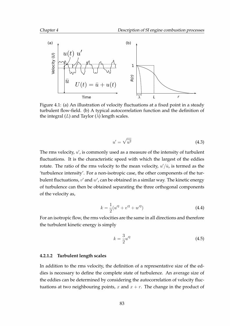
Chapter 4 Description of SI engine combustion processes
Time
Velo
cit
y (U
)
(a) (b)
R(r)
L r
1
Figure 4.1: (a) An illustration of velocity fluctuations at a fixed point in a steadyturbulent flow-field. (b) A typical autocorrelation function and the definition ofthe integral (L) and Taylor (λ) length scales.
u′ =√u2 (4.3)
The rms velocity, u′, is commonly used as a measure of the intensity of turbulentfluctuations. It is the characteristic speed with which the largest of the eddiesrotate. The ratio of the rms velocity to the mean velocity, u′/u, is termed as the‘turbulence intensity’. For a non-isotropic case, the other components of the tur-bulent fluctuations, v′ andw′, can be obtained in a similar way. The kinetic energyof turbulence can then be obtained separating the three orthogonal componentsof the velocity as,
k =1
2(u′2 + v′2 + w′2) (4.4)
For an isotropic flow, the rms velocities are the same in all directions and thereforethe turbulent kinetic energy is simply
k =3
2u′2 (4.5)
4.2.1.2 Turbulent length scales
In addition to the rms velocity, the definition of a representative size of the ed-dies is necessary to define the complete state of turbulence. An average size ofthe eddies can be determined by considering the autocorrelation of velocity fluc-tuations at two neighbouring points, x and x + r. The change in the product of
83
Chapter 4 Description of SI engine combustion processes
velocities at these two points, u(x)u(x+ r), as the distance r is increased gives anindication of the correlation between the local velocity fluctuations. The maxi-mum distance, upto which the two velocities are well correlated, gives a measureof the size of the largest eddies. A normalised spatial autocorrelation functionR(r) can be defined as:
R(r) =u(x)u(x+ r)
u′2(4.6)
The area under the autocorrelation function is given by the following inte-gral and gives a quantitative measure of the largest eddies and is known as theintegral length scale, L [Tennekes and Lumley, 1972]. It is equal to the widthof a rectangle of the same size as the area under the autocorrelation curve; seeFigure 4.1b.
L =
∫ ∞0
R(r)dr (4.7)
Determining the integral length scale by making a series of two simultaneousvelocity measurements at increasing distances by using methods such as the two-point LDV is rather difficult. A related quantity, the integral time scale, τL, canbe determined in a similar manner by making measurements at a single point atdifferent times if the Taylor hypothesis of frozen turbulence applies1. Thus anautocorrelation function in terms of time can be obtained as,
R(t) =u(t0)u(t0 + t)
u′2(4.8)
and the associated time scale known as the integral time scale can obtained as,
τL =
∫ ∞0
R(t)dt (4.9)
The integral time scale is the time taken by an eddy of size L to completeone rotation. Dimensional analysis provides the following relationship betweenintegral length scale and the integral time scale.
τL ∼L
u′(4.10)
1According to Taylor’s hypothesis, when the turbulence intensity (u′/u) is very small in asteady flow, multiple simultaneous measurements at various locations are equivalent to measure-ments taken at a single location at different times as the eddy advects through the probe alongthe flow.
84
Chapter 4 Description of SI engine combustion processes
As stated earlier, one of the definitive characteristics of turbulence is that it isdissipative due to viscous shear stresses. However, viscous forces play their roleat small scales across which the velocity gradients are large [Lipatnikov, 2013].Large vortices, of scale L, carry most of the kinetic energy and are largely unaf-fected by these viscous effects. They eventually break down to smaller eddies inwhich kinetic energy is dissipated to heat through viscous action at a rate givenby
ε ∼ u′3
L(4.11)
The length of these smaller eddies is given by the following expression due toKolmogorov [1941] and is known as the Kolmogorov microscale.
η = Cη
(ν3
ε
)1/4
(4.12)
where, Cη is a constant, of the order of unity [Borghi and Destriau, 1998] andν is the kinematic viscosity. Substituting for ε from equation (4.11) in the aboveequation, the expression can be written in terms of the Reynolds number as:
η = CηL
Re3/4(4.13)
and
Re =u′L
ν(4.14)
A length scale between the integral length scale and the Kolmogorov scale canbe defined by expanding the autocorrelation function, R(r), into a Taylor seriesand neglecting the higher order terms in the expansion. The remaining seriesgives a parabolic approximation of R as shown in Figure 4.1b and the distanceat which the parabola intersects the abscissa gives a characteristic length scaleknown as the Taylor microscale, [Taylor, 1915]. The Taylor microscale is given bythe expression:
λ = CλL
Re1/2(4.15)
Where,Cλ is a dimensionless constant whose value is suggested to be√
40.4 [R. G.Abdel-Gayed and Bradley, 1984].
From the discussion so far, it can be seen that the integral length scale and the
85
Chapter 4 Description of SI engine combustion processes
rms velocity provide a great deal of information about the state of turbulence.Therefore, a number of mathematical models have been proposed over the yearsfor their calculation. One such model is the k − ε model which is widely usedfor modelling turbulence in a variety of flows. It has also been employed in thiswork and is discussed in some detail in Section 4.7.1.
4.3 Background to combustion and flames
Combustion is an exothermic ensemble of reactions of a fuel and an oxidiser. Aflame is the region to which the combustion reactions are confined; often but notalways, the flame is luminous and in a premixed gaseous fuel-oxidiser mixture,it is self-propagating. This self sustained propagation of a flame usually occursat speeds much lower than the local sonic speed, such a flame is termed as a de-flagration wave. A flame which propagates at supersonic speeds is a detonation.Deflagration occurs through a gradual thermal and mass diffusion, whereas adetonation is a shock wave which is sustained by the energy liberated from com-bustion at a location through which the shock wave had passed.
The fuel-oxidiser contact necessary for the reactions to occur may take placebefore or after the ignition. If the fuel and oxidiser are premixed as in an SI engine,then the flame propagation is governed by the equilibrium between the chemicalreactions and molecular transport. If no mixing of the fuel and oxidiser occursbefore the ignition then the flame is anchored to the boundary between the fueland oxidiser and the heat release is governed by rate of mixing. Such flamesare referred to as diffusion flames and are relevant to diesel engines. The fueland oxidiser may also be partially premixed – diffusion and partially premixedflames have not been considered as they are out of the scope of this work.
The nature of the flame is greatly affected by interactions of flow-field and thereaction zone. The flame may be laminar or turbulent depending on the state ofturbulence. Turbulent flames are found in most of the practical applications suchas combustion engines, gas turbines, furnaces etc. Laminar flames have very lim-ited practical application, however, they are extensively studied for the insight itoffers into the burning characteristics of various fuels. In practical combustiondevices where turbulent flow conditions exist, the flame is distorted due to itsinteraction with the various turbulent eddies resulting in a propagation velocitywhich is not only a function of the laminar burning velocity, but the turbulencecharacteristics as well. Study of laminar premixed flames is therefore a prerequi-
86
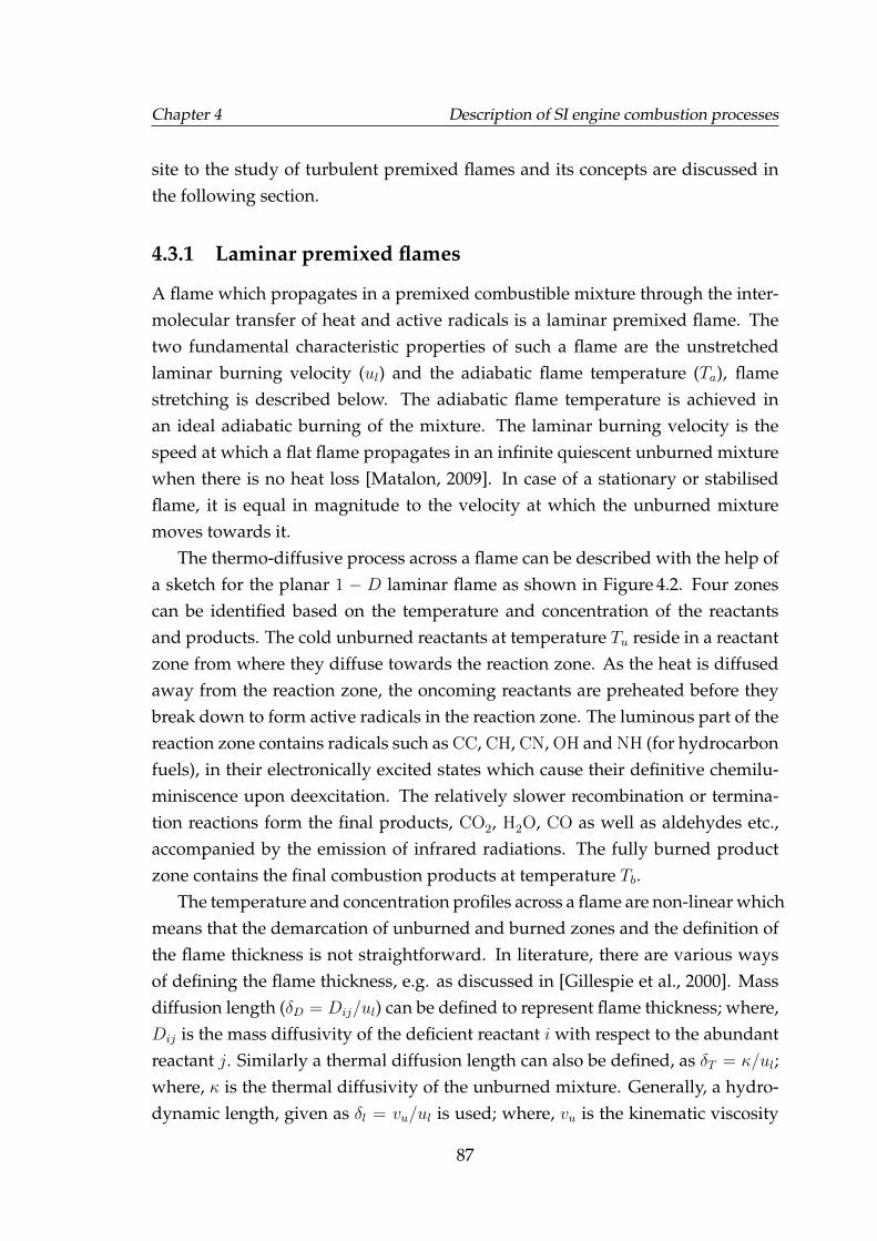
Chapter 4 Description of SI engine combustion processes
site to the study of turbulent premixed flames and its concepts are discussed inthe following section.
4.3.1 Laminar premixed flames
A flame which propagates in a premixed combustible mixture through the inter-molecular transfer of heat and active radicals is a laminar premixed flame. Thetwo fundamental characteristic properties of such a flame are the unstretchedlaminar burning velocity (ul) and the adiabatic flame temperature (Ta), flamestretching is described below. The adiabatic flame temperature is achieved inan ideal adiabatic burning of the mixture. The laminar burning velocity is thespeed at which a flat flame propagates in an infinite quiescent unburned mixturewhen there is no heat loss [Matalon, 2009]. In case of a stationary or stabilisedflame, it is equal in magnitude to the velocity at which the unburned mixturemoves towards it.
The thermo-diffusive process across a flame can be described with the help ofa sketch for the planar 1 − D laminar flame as shown in Figure 4.2. Four zonescan be identified based on the temperature and concentration of the reactantsand products. The cold unburned reactants at temperature Tu reside in a reactantzone from where they diffuse towards the reaction zone. As the heat is diffusedaway from the reaction zone, the oncoming reactants are preheated before theybreak down to form active radicals in the reaction zone. The luminous part of thereaction zone contains radicals such as CC, CH, CN, OH and NH (for hydrocarbonfuels), in their electronically excited states which cause their definitive chemilu-miniscence upon deexcitation. The relatively slower recombination or termina-tion reactions form the final products, CO2, H2O, CO as well as aldehydes etc.,accompanied by the emission of infrared radiations. The fully burned productzone contains the final combustion products at temperature Tb.
The temperature and concentration profiles across a flame are non-linear whichmeans that the demarcation of unburned and burned zones and the definition ofthe flame thickness is not straightforward. In literature, there are various waysof defining the flame thickness, e.g. as discussed in [Gillespie et al., 2000]. Massdiffusion length (δD = Dij/ul) can be defined to represent flame thickness; where,Dij is the mass diffusivity of the deficient reactant i with respect to the abundantreactant j. Similarly a thermal diffusion length can also be defined, as δT = κ/ul;where, κ is the thermal diffusivity of the unburned mixture. Generally, a hydro-dynamic length, given as δl = vu/ul is used; where, vu is the kinematic viscosity
87
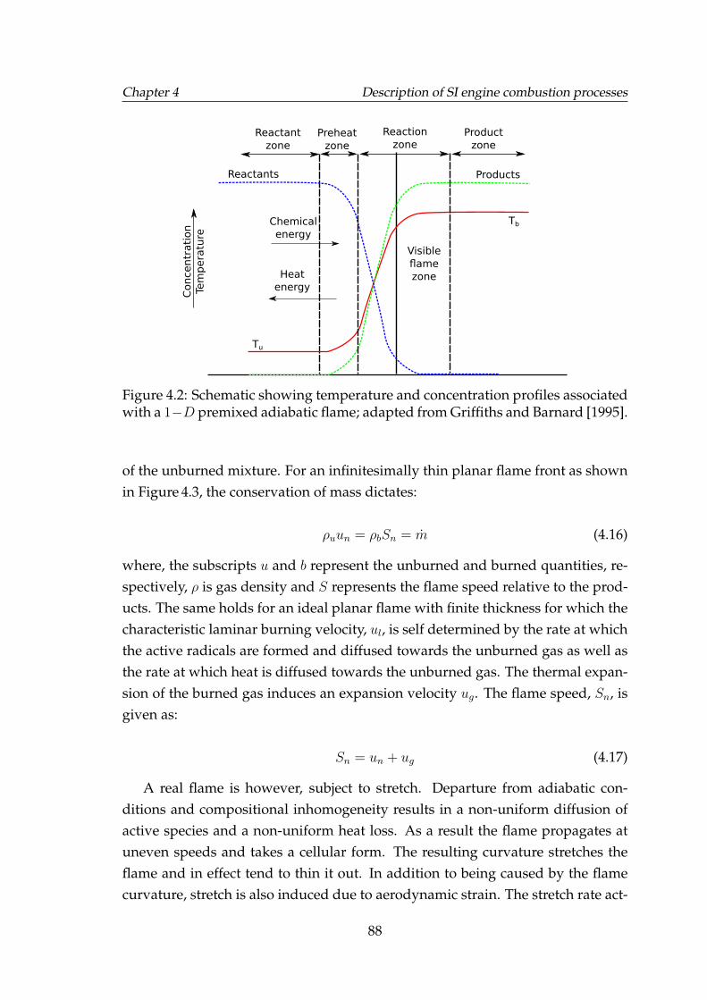
Chapter 4 Description of SI engine combustion processes
Tb
Tu
Reactants Products
Reactant
zone
Preheat
zone
Reaction
zoneProduct
zone
Concentr
ati
on
Tem
pera
ture
Chemical
energy
Heat
energy
Visible
flame
zone
Figure 4.2: Schematic showing temperature and concentration profiles associatedwith a 1−D premixed adiabatic flame; adapted from Griffiths and Barnard [1995].
of the unburned mixture. For an infinitesimally thin planar flame front as shownin Figure 4.3, the conservation of mass dictates:
ρuun = ρbSn = m (4.16)
where, the subscripts u and b represent the unburned and burned quantities, re-spectively, ρ is gas density and S represents the flame speed relative to the prod-ucts. The same holds for an ideal planar flame with finite thickness for which thecharacteristic laminar burning velocity, ul, is self determined by the rate at whichthe active radicals are formed and diffused towards the unburned gas as well asthe rate at which heat is diffused towards the unburned gas. The thermal expan-sion of the burned gas induces an expansion velocity ug. The flame speed, Sn, isgiven as:
Sn = un + ug (4.17)
A real flame is however, subject to stretch. Departure from adiabatic con-ditions and compositional inhomogeneity results in a non-uniform diffusion ofactive species and a non-uniform heat loss. As a result the flame propagates atuneven speeds and takes a cellular form. The resulting curvature stretches theflame and in effect tend to thin it out. In addition to being caused by the flamecurvature, stretch is also induced due to aerodynamic strain. The stretch rate act-
88
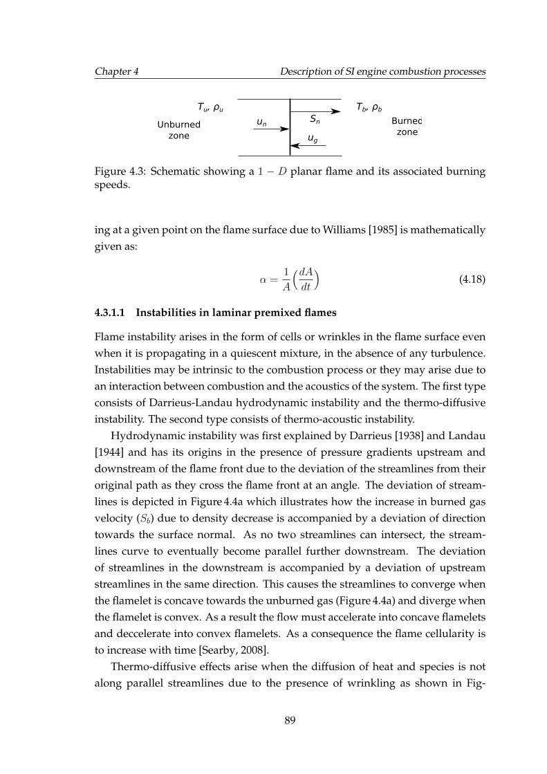
Chapter 4 Description of SI engine combustion processes
unSn
ug
Burned
zoneUnburned
zone
Tu, ρu Tb, ρb
Figure 4.3: Schematic showing a 1 − D planar flame and its associated burningspeeds.
ing at a given point on the flame surface due to Williams [1985] is mathematicallygiven as:
α =1
A
(dAdt
)(4.18)
4.3.1.1 Instabilities in laminar premixed flames
Flame instability arises in the form of cells or wrinkles in the flame surface evenwhen it is propagating in a quiescent mixture, in the absence of any turbulence.Instabilities may be intrinsic to the combustion process or they may arise due toan interaction between combustion and the acoustics of the system. The first typeconsists of Darrieus-Landau hydrodynamic instability and the thermo-diffusiveinstability. The second type consists of thermo-acoustic instability.
Hydrodynamic instability was first explained by Darrieus [1938] and Landau[1944] and has its origins in the presence of pressure gradients upstream anddownstream of the flame front due to the deviation of the streamlines from theiroriginal path as they cross the flame front at an angle. The deviation of stream-lines is depicted in Figure 4.4a which illustrates how the increase in burned gasvelocity (Sb) due to density decrease is accompanied by a deviation of directiontowards the surface normal. As no two streamlines can intersect, the stream-lines curve to eventually become parallel further downstream. The deviationof streamlines in the downstream is accompanied by a deviation of upstreamstreamlines in the same direction. This causes the streamlines to converge whenthe flamelet is concave towards the unburned gas (Figure 4.4a) and diverge whenthe flamelet is convex. As a result the flow must accelerate into concave flameletsand deccelerate into convex flamelets. As a consequence the flame cellularity isto increase with time [Searby, 2008].
Thermo-diffusive effects arise when the diffusion of heat and species is notalong parallel streamlines due to the presence of wrinkling as shown in Fig-
89
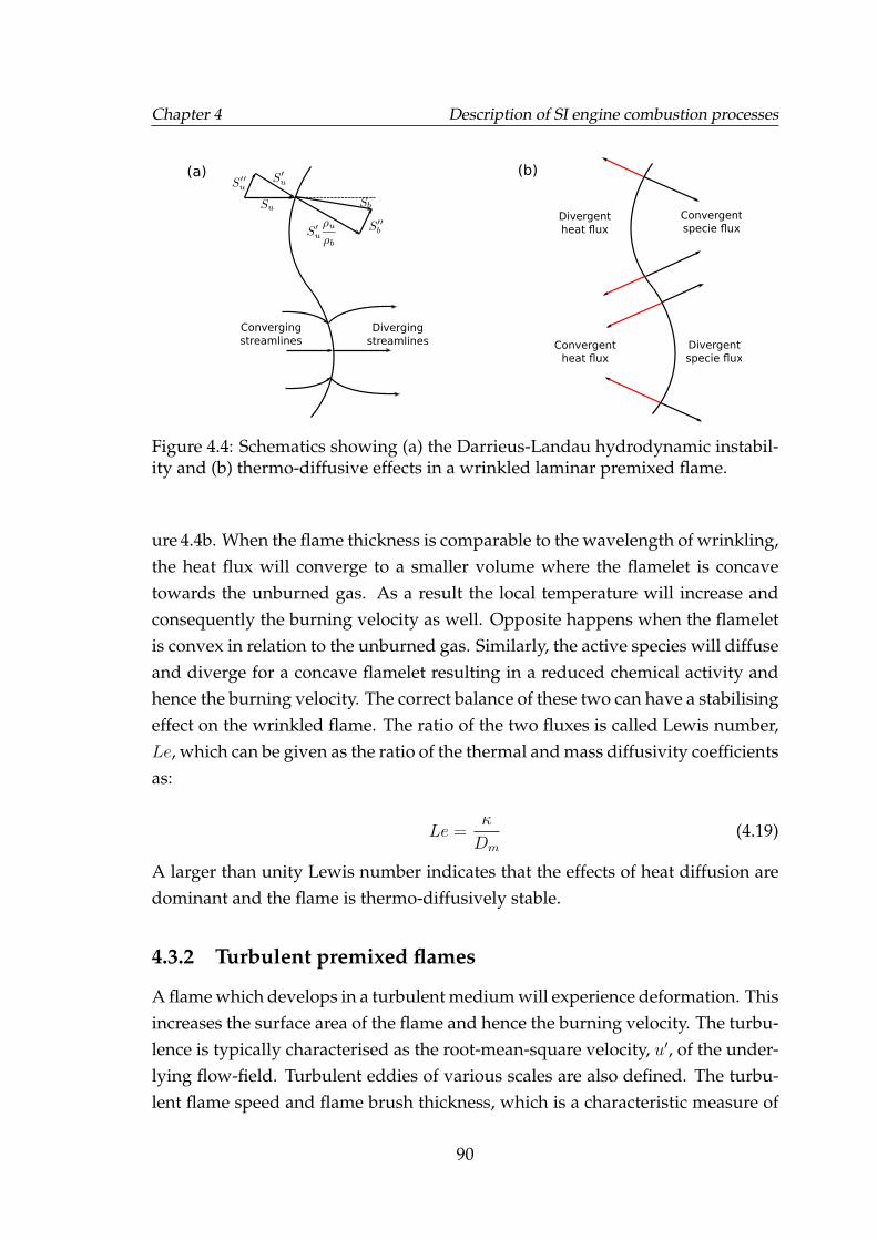
Chapter 4 Description of SI engine combustion processes
Converging
streamlines
Diverging
streamlines
Divergent
heat flux
Convergent
heat flux
Convergent
specie flux
Divergent
specie flux
(a) (b)
Figure 4.4: Schematics showing (a) the Darrieus-Landau hydrodynamic instabil-ity and (b) thermo-diffusive effects in a wrinkled laminar premixed flame.
ure 4.4b. When the flame thickness is comparable to the wavelength of wrinkling,the heat flux will converge to a smaller volume where the flamelet is concavetowards the unburned gas. As a result the local temperature will increase andconsequently the burning velocity as well. Opposite happens when the flameletis convex in relation to the unburned gas. Similarly, the active species will diffuseand diverge for a concave flamelet resulting in a reduced chemical activity andhence the burning velocity. The correct balance of these two can have a stabilisingeffect on the wrinkled flame. The ratio of the two fluxes is called Lewis number,Le, which can be given as the ratio of the thermal and mass diffusivity coefficientsas:
Le =κ
Dm
(4.19)
A larger than unity Lewis number indicates that the effects of heat diffusion aredominant and the flame is thermo-diffusively stable.
4.3.2 Turbulent premixed flames
A flame which develops in a turbulent medium will experience deformation. Thisincreases the surface area of the flame and hence the burning velocity. The turbu-lence is typically characterised as the root-mean-square velocity, u′, of the under-lying flow-field. Turbulent eddies of various scales are also defined. The turbu-lent flame speed and flame brush thickness, which is a characteristic measure of
90
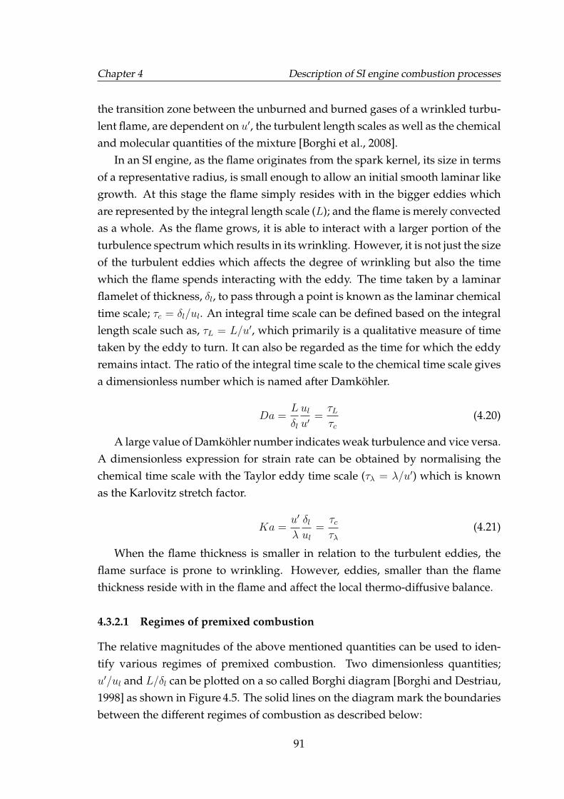
Chapter 4 Description of SI engine combustion processes
the transition zone between the unburned and burned gases of a wrinkled turbu-lent flame, are dependent on u′, the turbulent length scales as well as the chemicaland molecular quantities of the mixture [Borghi et al., 2008].
In an SI engine, as the flame originates from the spark kernel, its size in termsof a representative radius, is small enough to allow an initial smooth laminar likegrowth. At this stage the flame simply resides with in the bigger eddies whichare represented by the integral length scale (L); and the flame is merely convectedas a whole. As the flame grows, it is able to interact with a larger portion of theturbulence spectrum which results in its wrinkling. However, it is not just the sizeof the turbulent eddies which affects the degree of wrinkling but also the timewhich the flame spends interacting with the eddy. The time taken by a laminarflamelet of thickness, δl, to pass through a point is known as the laminar chemicaltime scale; τc = δl/ul. An integral time scale can be defined based on the integrallength scale such as, τL = L/u′, which primarily is a qualitative measure of timetaken by the eddy to turn. It can also be regarded as the time for which the eddyremains intact. The ratio of the integral time scale to the chemical time scale givesa dimensionless number which is named after Damkohler.
Da =L
δl
ulu′
=τLτc
(4.20)
A large value of Damkohler number indicates weak turbulence and vice versa.A dimensionless expression for strain rate can be obtained by normalising thechemical time scale with the Taylor eddy time scale (τλ = λ/u′) which is knownas the Karlovitz stretch factor.
Ka =u′
λ
δlul
=τcτλ
(4.21)
When the flame thickness is smaller in relation to the turbulent eddies, theflame surface is prone to wrinkling. However, eddies, smaller than the flamethickness reside with in the flame and affect the local thermo-diffusive balance.
4.3.2.1 Regimes of premixed combustion
The relative magnitudes of the above mentioned quantities can be used to iden-tify various regimes of premixed combustion. Two dimensionless quantities;u′/ul and L/δl can be plotted on a so called Borghi diagram [Borghi and Destriau,1998] as shown in Figure 4.5. The solid lines on the diagram mark the boundariesbetween the different regimes of combustion as described below:
91
Chapter 4 Description of SI engine combustion processes
0.1 1 10 100 1000L/δ
l
0.1
1
10
100
u’/u
l
Laminar flames
Well-stirred reactor(thick flame with distributed combustion) Distributed reaction zone
(thickened, wrinkled flamewith possible extinction)
Corrugated flamelets(wrinkled flame with pockets)
Wrinkled flamelets
Re = 1
τ c = τ λ
or Ka = 1
τc < τ
λ
τL > τ
c > τ
λ
τc > τ
L
τ c =
τ L o
r Da
= 1Da < 1
Ka < 1
Figure 4.5: Borghi diagram
• Laminar flames (Re < 1): The flame is laminar as the turbulence is weakand the size of eddies is smaller than the flame thickness and therefore doesnot cause any wrinkling of the flame.
• Wrinkled flamelet regime (Re > 1, Ka < 1, u′ < ul): These conditionspertain to a wrinkled flamelet regime. The integral length scale, L, is largerthan the flame thickness and causes the flame to wrinkle. However, theturbulence is not strong enough to cause any folding or stretching of theflame surface. The chemical time scale is shorter than the Taylor eddy timescale which means that the smaller eddies are able to burn before they breakdown. As a result each flamelet or cell burns in a similar way as a laminarflame. It has also been widely argued that a turbulent flame can be treatedas an array of laminar flamelets within which no turbulence structures exist[Bradley, 1992] and considerable experimental evidence in support of thisview has been produced, see [Warnatz et al., 2001, p. 204] but this holdstrue for conditions when the Damkohler number is large as in this wrin-kled flamelet regime. This clearly is irrelevant to combustion in SI engineswhere a simplification assumption like that of the laminar flamelets willnot explain the flame perturbations caused by the smaller turbulent lengthscales.
92
Chapter 4 Description of SI engine combustion processes
• Corrugated flamelet regime (Re > 1, Ka < 1, u′ > ul): Turbulence intensityis higher in comparison to the local laminar flame speed. As a result theflame is not only wrinkled but folded on itself resulting in the formation ofpockets of unburned mixture on the burned side and vice versa. Flames inSI engines tend to be in this wrinkled-corrugated regime.
• Distributed reaction zone (Re > 1, Ka > 1, Da > 1): As τc > τλ, there isinsufficient time for the eddies to burn. This results in a greater stretchingand breaking up of the flame resulting in distributed reaction zones. Theresultant flame is also much thickened.
• Thickened flames, well-stirred reactor (Re > 1, Ka > 1, Da < 1): Thechemical life time is longer than the life time of even the biggest eddies.The flame is continuously stretched and broken up resulting in localisedextinctions.
4.4 Modelling of combustion in SI engines
The prime objective of engine combustion modelling is to be able to predict themass burning rate of the air-fuel charge on which the engine performance calcula-tions rely. Several approaches exist for the simulation of the combustion processand are generally classified as zero, multi-zone and multi-dimensional. Burluka[2010] presented an overview of the thermodynamic modelling approach whichis the approach taken in the present work and forms the basis for The Univer-sity of Leeds engine modelling code ‘Leeds University Spark Ignition Engine’ orLUSIE for short. Zero dimensional representation of the combustion process ne-glects the spatial details and therefore the thermodynamic state of the in-cylindergases is only a function of time. Multi-zone approach builds on the same prin-ciple but differentiates between a burned and an unburned zone by defining athin reaction zone or a flame front separating the two zones each characterizedby its own thermodynamic state and composition. Multi-dimensional modelsaccount for the detailed fluid dynamics and its interaction with the combustionchemistry and therefore the governing equations are a function of space and timemaking the solution computationally expensive. Where the importance of multi-dimensional modelling is incontestable, the development of models for the multi-zone approach is of considerable importance as it allows a fast analysis of theeffects of various engine design parameters on engine performance.
93
Chapter 4 Description of SI engine combustion processes
4.5 Zero/multi-zone thermodynamic modelling
Over the years, thermodynamic models governing various SI engine phenom-ena have been implemented in a Fortran code at The University of Leeds as alibrary referred to as LUSIE, the groundwork for which was laid out in [Hynes,1986]. Models comprised in LUSIE are described in detail later in Section 4.6; fora brief history of LUSIE development, the interested reader is directed to [Con-way, 2013]. Hattrell [2007] combined the combustion routines of LUSIE which isa closed cycle code with GT-Power which offers versatile capabilities of 1-D mod-elling of the gas exchange process. The resulting hybrid modelling environmentis referred to as GT-LU. The present work is the continuation of the developmentof predictive modelling tools for engine design, particular emphasis here is onmodelling autoignition in the end gas with realistic hydrocarbon oxidation re-action kinetics. The significant contribution of the present work to LUSIE andGT-LU is the development of subroutines for the chemical reaction kinetics.
4.5.1 Zero dimensional thermodynamic modelling
The zero dimensional approach assumes the conversion of the air-fuel charge tofinal combustion products in a single step. The reaction rate is given by an empir-ical expression often containing adjustable parameters. The so-called Wiebe func-tion, i.e. a zero-dimensional model proposed by Ivan Wiebe in 1954 was basedon the assumption that the detailed chemical reaction kinetics can be reduced toa generic macroscopic reaction rate expression for engineering applications. TheWiebe function is still very often used in engine modelling as it offers unrivalledconvergence and computational speed. But the same nature which makes its useadvantageous is the cause of its inherent weakness. The Wiebe function is anempirical one which is defined for one particular engine condition and its extrap-olation to other conditions is difficult. A review on the subject has been presentedby Ghojel [2010]. Multi-zone thermodynamic modelling of the SI engines may of-fer a better accuracy of burn rate predictions at feasible computational speeds.
4.5.2 Two-zone thermodynamic modelling
Two-zone modelling is the simplest of the zonal modelling approaches as it as-sumes the in-cylinder charge to have been divided into a burned and an un-burned zone. This implies that the zonal boundary is an infinitesimally thin
94
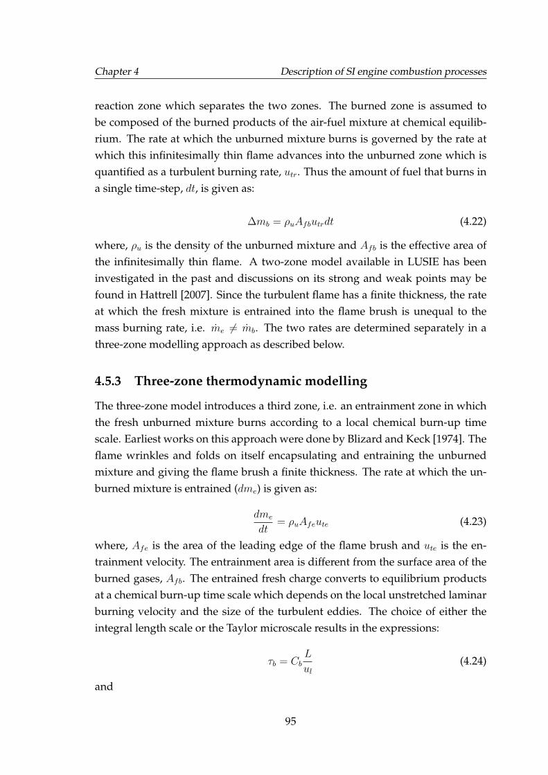
Chapter 4 Description of SI engine combustion processes
reaction zone which separates the two zones. The burned zone is assumed tobe composed of the burned products of the air-fuel mixture at chemical equilib-rium. The rate at which the unburned mixture burns is governed by the rate atwhich this infinitesimally thin flame advances into the unburned zone which isquantified as a turbulent burning rate, utr. Thus the amount of fuel that burns ina single time-step, dt, is given as:
∆mb = ρuAfbutrdt (4.22)
where, ρu is the density of the unburned mixture and Afb is the effective area ofthe infinitesimally thin flame. A two-zone model available in LUSIE has beeninvestigated in the past and discussions on its strong and weak points may befound in Hattrell [2007]. Since the turbulent flame has a finite thickness, the rateat which the fresh mixture is entrained into the flame brush is unequal to themass burning rate, i.e. me 6= mb. The two rates are determined separately in athree-zone modelling approach as described below.
4.5.3 Three-zone thermodynamic modelling
The three-zone model introduces a third zone, i.e. an entrainment zone in whichthe fresh unburned mixture burns according to a local chemical burn-up timescale. Earliest works on this approach were done by Blizard and Keck [1974]. Theflame wrinkles and folds on itself encapsulating and entraining the unburnedmixture and giving the flame brush a finite thickness. The rate at which the un-burned mixture is entrained (dme) is given as:
dme
dt= ρuAfeute (4.23)
where, Afe is the area of the leading edge of the flame brush and ute is the en-trainment velocity. The entrainment area is different from the surface area of theburned gases, Afb. The entrained fresh charge converts to equilibrium productsat a chemical burn-up time scale which depends on the local unstretched laminarburning velocity and the size of the turbulent eddies. The choice of either theintegral length scale or the Taylor microscale results in the expressions:
τb = CbL
ul(4.24)
and
95
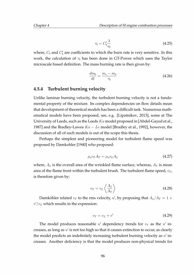
Chapter 4 Description of SI engine combustion processes
τb = C ′bλ
ul(4.25)
where, Cb and C ′b are coefficients to which the burn rate is very sensitive. In thiswork, the calculation of τb has been done in GT-Power which uses the Taylormicroscale based definition. The mass burning rate is then given by:
dmb
dt=me −mb
τb(4.26)
4.5.4 Turbulent burning velocity
Unlike laminar burning velocity, the turbulent burning velocity is not a funda-mental property of the mixture. Its complex dependencies on flow details meanthat development of theoretical models has been a difficult task. Numerous math-ematical models have been proposed, see, e.g. [Lipatnikov, 2013], some at TheUniversity of Leeds, such as the LeedsKamodel proposed in [Abdel-Gayed et al.,1987] and the Bradley-Lawes Ka − Le model [Bradley et al., 1992], however, thediscussion of all of such models is out of the scope this thesis.
Perhaps the simplest and pioneering model for turbulent flame speed wasproposed by Damkohler [1940] who proposed:
ρuvTAT = ρuvLAL (4.27)
where, AL is the overall area of the wrinkled flame surface, whereas, AT is meanarea of the flame front within the turbulent brush. The turbulent flame speed, vT ,is therefore given by:
vT = vL
⟨ALAT
⟩(4.28)
Damkohler related vT to the rms velocity, u′, by proposing that AL/AT = 1 +
v′/vL which results in the expression:
vT = vL + v′ (4.29)
The model produces reasonable u′ dependency trends for vT as the u′ in-creases, as long as u′ is not too high so that it causes extinction to occur, as clearlythe model predicts an indefinitely increasing turbulent burning velocity as u′ in-creases. Another deficiency is that the model produces non-physical trends for
96
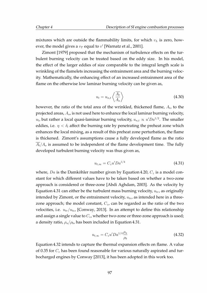
Chapter 4 Description of SI engine combustion processes
mixtures which are outside the flammability limits, for which vL is zero, how-ever, the model gives a vT equal to v′ [Warnatz et al., 2001].
Zimont [1979] proposed that the mechanism of turbulence effects on the tur-bulent burning velocity can be treated based on the eddy size. In his model,the effect of the larger eddies of size comparable to the integral length scale iswrinkling of the flamelets increasing the entrainment area and the burning veloc-ity. Mathematically, the enhancing effect of an increased entrainment area of theflame on the otherwise low laminar burning velocity can be given as,
ut = un,t
⟨AtAo
⟩(4.30)
however, the ratio of the total area of the wrinkled, thickened flame, At, to theprojected areas,Ao, is not used here to enhance the local laminar burning velocity,ul, but rather a local quasi-laminar burning velocity, un,t ∝ u′Da1/2. The smallereddies, i.e. η < δl affect the burning rate by penetrating the preheat zone whichenhances the local mixing, as a result of this preheat zone perturbation, the flameis thickened. Zimont’s assumptions cause a fully developed flame as the ratioAt/Ao is assumed to be independent of the flame development time. The fullydeveloped turbulent burning velocity was thus given as,
ut,∞ = Czu′Da1/4 (4.31)
where, Da is the Damkohler number given by Equation 4.20, Cz is a model con-stant for which different values have to be taken based on whether a two-zoneapproach is considered or three-zone [Abdi Aghdam, 2003]. As the velocity byEquation 4.31 can either be the turbulent mass burning velocity, utr, as originallyintended by Zimont, or the entrainment velocity, ute, as intended here in a three-zone approach; the model constant, Cz, can be regarded as the ratio of the twovelocities, i.e. utr/ute, [Conway, 2013]. In an attempt to define this relationshipand assign a single value toCz, whether two-zone or three-zone approach is used;a density ratio, ρu/ρb, has been included in Equation 4.31.
ut,∞ = Czu′Da1/4ρu
ρb(4.32)
Equation 4.32 intends to capture the thermal expansion effects on flame. A valueof 0.35 for Cz has been found reasonable for various naturally aspirated and tur-bocharged engines by Conway [2013], it has been adopted in this work too.
97
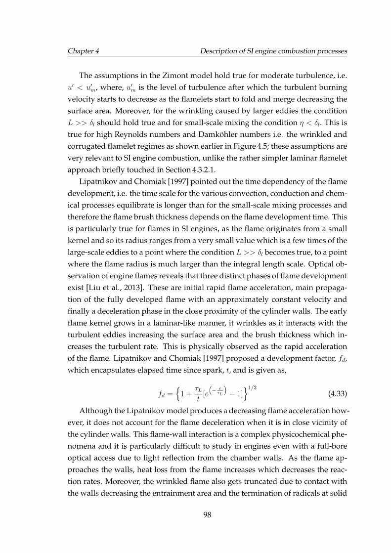
Chapter 4 Description of SI engine combustion processes
The assumptions in the Zimont model hold true for moderate turbulence, i.e.u′ < u′m, where, u′m is the level of turbulence after which the turbulent burningvelocity starts to decrease as the flamelets start to fold and merge decreasing thesurface area. Moreover, for the wrinkling caused by larger eddies the conditionL >> δl should hold true and for small-scale mixing the condition η < δl. This istrue for high Reynolds numbers and Damkohler numbers i.e. the wrinkled andcorrugated flamelet regimes as shown earlier in Figure 4.5; these assumptions arevery relevant to SI engine combustion, unlike the rather simpler laminar flameletapproach briefly touched in Section 4.3.2.1.
Lipatnikov and Chomiak [1997] pointed out the time dependency of the flamedevelopment, i.e. the time scale for the various convection, conduction and chem-ical processes equilibrate is longer than for the small-scale mixing processes andtherefore the flame brush thickness depends on the flame development time. Thisis particularly true for flames in SI engines, as the flame originates from a smallkernel and so its radius ranges from a very small value which is a few times of thelarge-scale eddies to a point where the condition L >> δl becomes true, to a pointwhere the flame radius is much larger than the integral length scale. Optical ob-servation of engine flames reveals that three distinct phases of flame developmentexist [Liu et al., 2013]. These are initial rapid flame acceleration, main propaga-tion of the fully developed flame with an approximately constant velocity andfinally a deceleration phase in the close proximity of the cylinder walls. The earlyflame kernel grows in a laminar-like manner, it wrinkles as it interacts with theturbulent eddies increasing the surface area and the brush thickness which in-creases the turbulent rate. This is physically observed as the rapid accelerationof the flame. Lipatnikov and Chomiak [1997] proposed a development factor, fd,which encapsulates elapsed time since spark, t, and is given as,
fd ={
1 +τLt
[e
(− tτL
)− 1]
}1/2
(4.33)
Although the Lipatnikov model produces a decreasing flame acceleration how-ever, it does not account for the flame deceleration when it is in close vicinity ofthe cylinder walls. This flame-wall interaction is a complex physicochemical phe-nomena and it is particularly difficult to study in engines even with a full-boreoptical access due to light reflection from the chamber walls. As the flame ap-proaches the walls, heat loss from the flame increases which decreases the reac-tion rates. Moreover, the wrinkled flame also gets truncated due to contact withthe walls decreasing the entrainment area and the termination of radicals at solid
98
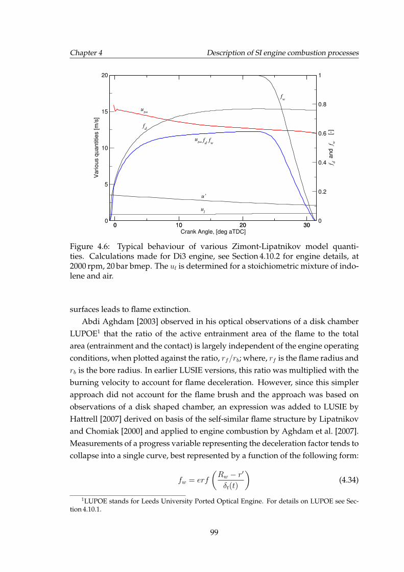
Chapter 4 Description of SI engine combustion processes
0 10 20 30Crank Angle, [deg aTDC]
0
5
10
15
20
Various q
uantities [m
/s]
0 10 20 300
0.2
0.4
0.6
0.8
1
f dand f w
[-
]
ut∞
fw
fd
ut∞
u’
ul
fdfw
Figure 4.6: Typical behaviour of various Zimont-Lipatnikov model quanti-ties. Calculations made for Di3 engine, see Section 4.10.2 for engine details, at2000 rpm, 20 bar bmep. The ul is determined for a stoichiometric mixture of indo-lene and air.
surfaces leads to flame extinction.Abdi Aghdam [2003] observed in his optical observations of a disk chamber
LUPOE1 that the ratio of the active entrainment area of the flame to the totalarea (entrainment and the contact) is largely independent of the engine operatingconditions, when plotted against the ratio, rf/rb; where, rf is the flame radius andrb is the bore radius. In earlier LUSIE versions, this ratio was multiplied with theburning velocity to account for flame deceleration. However, since this simplerapproach did not account for the flame brush and the approach was based onobservations of a disk shaped chamber, an expression was added to LUSIE byHattrell [2007] derived on basis of the self-similar flame structure by Lipatnikovand Chomiak [2000] and applied to engine combustion by Aghdam et al. [2007].Measurements of a progress variable representing the deceleration factor tends tocollapse into a single curve, best represented by a function of the following form:
fw = erf
(Rw − r′
δt(t)
)(4.34)
1LUPOE stands for Leeds University Ported Optical Engine. For details on LUPOE see Sec-tion 4.10.1.
99
Chapter 4 Description of SI engine combustion processes
Where Rw is the bore radius and r′ is the current flame radius. The flame brushthickness, δt, is governed by turbulent diffusion and is given by Lipatnikov andChomiak [2000] as:
δt(t) = u′τL
{2t′[1− 1
t′(1− e−t′)
]}1/2
(4.35)
Where t′ is a dimensionless time given by t/τL.The entrainment velocity, ute, required for the mass entrainment rate in equa-
tion (4.23) is given by the expression:
ute = (ul + ut,∞fd)fw (4.36)
Figure 4.6 shows graphically various quantities which have been discussed sofar. Since the flame which has a characteristic laminar burning velocity, ul, is sub-jected to turbulence of intensity, u′, consequentially its fully developed turbulentburning velocity, ut0, is much higher than ul and is shown by the red line. How-ever, in an engine, this equilibrium velocity is not achieved instantaneously atthe inception of the flame. The initial flame acceleration is accounted for by thedevelopment factor, fd, and the final deceleration due to wall proximity by, fw.These factors when multiplied to ut0 produce the expected three stages of flamepropagation, shown in blue.
The Zimont-Lipatnikov model has been extensively studied in Lipatnikov andChomiak [2002] as well as Abdi Aghdam [2003] who made a comparison withthe Leeds Ka and KaLe models and found that the models performed similarlywell, however, the Zimont-Lipatnikov model performed better at different com-pression ratios, equivalence ratios and speeds of the naturally aspirated LUPOE.The model has previously been found to perform well for a variety of enginesand operating conditions and it has been adopted in this work as well. However,most of the previous applications of this model have been to naturally aspiratedengines and it must be pointed out that with extreme pressure charging of en-gines, there is a need for an investigation into the validity of the Zimont model tosuch modern turbocharged engines. In this work the model has been applied toa turbocharged SI engine.
100
Chapter 4 Description of SI engine combustion processes
4.6 Introduction to LUSIE
LUSIE is a collection of models which simulate the closed part of the engine cycleincluding the compression and expansion by modelling its various physicochem-ical processes in a sequential manner. This is done by dividing the whole durationof the firing cycle in small discrete time steps. For every incremental change inthe time the piston movement is calculated and the corresponding volume andresulting pressure changes as well. Specialized routines calculate the flow char-acteristics, combustion rate, chemical equilibrium composition, heat transfer andblowby etc. An excellent description of the LUSIE models and its way of opera-tion has been presented by Hattrell [2007] and Conway [2013]. A brief overviewof these routines/models is presented in the following sections leading up to adescription of GT-LU which is the main research tool used in the present work.
4.6.1 Motoring simulation
Each LUSIE simulation run begins by first performing a motoring simulation ofthe cycle. This is done by simply calculating the polytropic compression pressureand temperature as the combustion chamber volume changes because of the pis-ton motion. The in-cylinder composition is assumed to be frozen. The heat lossto the walls is calculated and the mass lost due to blowby as well.
4.6.2 Heat transfer
The dominant mode of heat transfer between the combustion gases and the en-gine chamber walls in SI engines is convection. Heat flux varies from surface tosurface and may reach values of 10 MW/m2 at the interface of the burned gas andthe chamber walls, known as the wetted area, [Heywood, 1988]. Numerous for-mulas exist for instantaneous convective heat transfer coefficient which originatefrom the Nusselt-Reynolds relationships for turbulent flows in pipes. Correla-tions of Annand [1963] and Woschni [1967] are used in LUSIE as in many otherengine simulation packages. Details on the implementation of these correlationsin LUSIE can be seen in [Abdi Aghdam, 2003], [Liu, 2004], [Hattrell, 2007] and[Conway, 2013].
101
Chapter 4 Description of SI engine combustion processes
4.6.3 Blowby
Pressure in the crank case remains much lower than the compression and com-bustion pressures in the cylinder. The in-cylinder gases tend to leak through thegap between the piston and the liner. This flow is minimised by machining thepiston and the liner to very close tolerances to achieve the tightest possible fit.Additional sealing is provided by installing a set of rings on the piston whichprovide even tighter seal without excessive friction and a dedicated oil scrap-per ring also helps in maintaining a film of lubricant. Modern production en-gines have low levels of blowby and therefore a good prediction of the cylinderpressures can be achieved even in the absence of a blowby model. LUPOE2-D,see Section 4.10.1 for details on the engine, however, has considerable amount ofblowby (about 10% from previous studies on LUPOE1 [Abdi Aghdam, 2003]) andtherefore blowby is modelled for LUPOE2-D simulations only.
LUSIE includes a blowby model which simulates the leakage of in-cylindergases by an expression for compressible isentropic flow of gas though an orifice.The derivation of the expression can be seen in Appendix C of [Heywood, 1988]and details on its implementation in LUSIE can be found in [Abdi Aghdam, 2003]and [Hattrell, 2007]. In LUSIE a distinction is made between the part of blowbymass which permanently escapes the combustion chamber and a portion whichre-enters the combustion chamber during the late stages of combustion duringthe expansion stroke.
4.6.4 Laminar burning velocity
For SI engine modelling, the laminar burning velocity can be most accuratelydetermined by using empirical correlations derived from experimental measure-ments in a spherical vessel of the flame radius and associated pressure rise asa laminar flame propagates radially outwards from a central spark [Heywood,1988]. Measurements can be found in the literature for laminar burning veloc-ities of methane, propane, iso-octane, gasoline and methanol, at various enginerelevant pressures, temperature and compositions. A power law expression byMetghalchi and Keck [1982] has been used in LUSIE as well as GT-Power and isgiven as,
ul =(Bm +Bφ(φ− φm)2
)(TuT0
)α
(p
p0
)β(1− 2.06(Dilution)0.77) (4.37)
102
Chapter 4 Description of SI engine combustion processes
where, Bm is the maximum velocity at an equivalence ratio φm. The in-cylinderequivalence ratio is φ, Tu is the unburned gas temperature and T0 and p0 arestandard temperature and pressure, 300 K and 1 atm respectively. Dilution refersto the mass fraction of the residuals in the unburned zone. The temperature andpressure exponents, α and β, and the other model constants for gasoline whichare used in this work are based on the works of Takashi and Kimitoshi [2006] andare given as:
Bm [m/s] Bφ [m/s] φm α β0.350 -0.549 1.1 2.4 - 0.271 φ3.51 -0.357 + 0.14 φ2.77
4.6.5 Autoignition modelling
Autoignition modelling is key to the prediction of knock occurrence during thedevelopment phase of an engine design and this is one of the main objectives ofthis work. As discussed in Chapter 2, chemical reaction kinetics has been em-ployed to predict the end gas autoignition. Prior to the use of detailed chemicalkinetic mechanisms, an empirical expression and skeletal mechanisms have longbeen used in LUSIE and GT-LU. A widely used empirical model is by Douaudand Eyzat [1978], commonly known as the D&E model and it has been intro-duced earlier in Section 1.6. Among the skeletal models are the renowned ‘Shell’model by Halstead et al. [1977] as well as the model by Chun et al. [1989] andits refinements, e.g. [Cowart et al., 1991] and [Nishiwaki et al., 2000], were pre-viously used for autoignition with reasonable success. These mechanisms havebeen discussed in Chapter 2, discussion here is reserved only for the coupling ofchemistry solver with LUSIE and GT-LU.
The autoignition modelling approach in this work involves modelling of theoxidation chemistry of the air-fuel mixture in the end gas by using the chemistrysolver discussed earlier in Section 2.4. The chemistry calculations are performedat each time step (or the crank degree increment) of the main engine cycle sim-ulation. The inputs required for the chemistry modelling are the pressure, tem-perature, volume and initial composition of the end gas. On every call to theautoignition subroutine, the change in concentration of each species and the newend gas temperature is determined. The new unburned zone temperature is fedback to the main cycle simulation and the species concentrations are saved for thenext iteration, see Figure 4.7. Same procedure is carried out for subsequent timesteps, however, the saved specie concentrations from the previous time step are
103
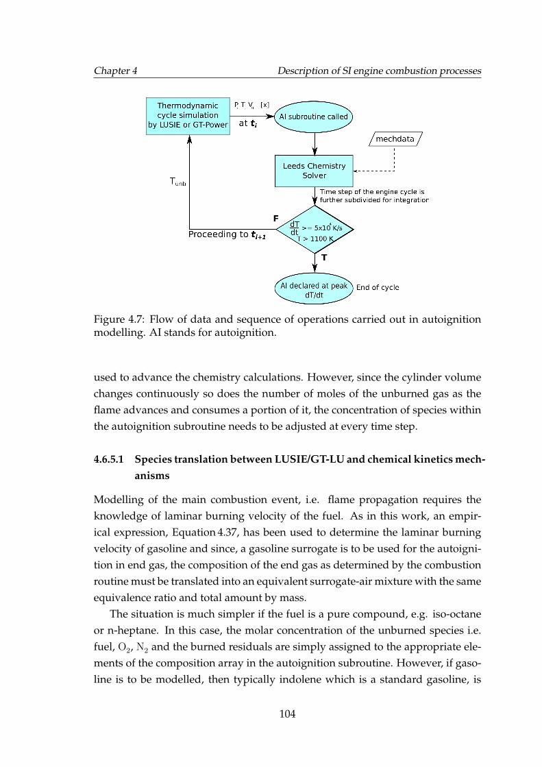
Chapter 4 Description of SI engine combustion processes
AI subroutine called
Leeds Chemistry
Solver
dT>= 5x10 K/s
dt
4
T > 1100 K
[x]Tu
Pu
Vu
T
F
End of cycle AI declared at peak
dT/dt
Figure 4.7: Flow of data and sequence of operations carried out in autoignitionmodelling. AI stands for autoignition.
used to advance the chemistry calculations. However, since the cylinder volumechanges continuously so does the number of moles of the unburned gas as theflame advances and consumes a portion of it, the concentration of species withinthe autoignition subroutine needs to be adjusted at every time step.
4.6.5.1 Species translation between LUSIE/GT-LU and chemical kinetics mech-anisms
Modelling of the main combustion event, i.e. flame propagation requires theknowledge of laminar burning velocity of the fuel. As in this work, an empir-ical expression, Equation 4.37, has been used to determine the laminar burningvelocity of gasoline and since, a gasoline surrogate is to be used for the autoigni-tion in end gas, the composition of the end gas as determined by the combustionroutine must be translated into an equivalent surrogate-air mixture with the sameequivalence ratio and total amount by mass.
The situation is much simpler if the fuel is a pure compound, e.g. iso-octaneor n-heptane. In this case, the molar concentration of the unburned species i.e.fuel, O2, N2 and the burned residuals are simply assigned to the appropriate ele-ments of the composition array in the autoignition subroutine. However, if gaso-line is to be modelled, then typically indolene which is a standard gasoline, is
104
Chapter 4 Description of SI engine combustion processes
used to simulate the flame propagation event. It is common practice to adjust thecalorific value and the stoichiometric air-to-fuel ratio of indolene to match that ofthe target gasoline. Translating the unburned gas composition, indolene, air andresiduals, to the species in autoignition subroutine is not that straightforward.
Since we are simulating the autoignition behaviour of gasoline by means of asurrogate, the underlying assumption is that the surrogate must replace gasolineat the same equivalence ratio. Splitting the concentration or moles of gasolinein the unburned gas into the surrogate components based on its molar compo-sition will only be acceptable if the C/H/O atomic proportion of indolene is thesame as that of the surrogate. Or in other words, the surrogate has the same sto-ichiometric air-to-fuel ratio, A/Fst, as the target gasoline. It is for this reason thatmatching of A/Fst was emphasised in Section 2.9. However, it may not always bepossible to formulate a surrogate with the same stoichiometric air-to-fuel ratio asthe target gasoline. The best approach, and the one which is used in this work, isto recalculate the surrogate-air composition according to the prevailing equiva-lence ratio regardless of whether the A/Fst was matched or not while conservingthe total mass of unburned charge.
4.6.5.2 Autoignition criteria
The instant at which autoignition is said to have occurred is when there is a sharpincrease of temperature. Halstead et al. [1977] used an arbitrary threshold valueof 107 K/s for the rate of temperature rise or the temperature value of 1100 K. Asimilar criteria of two conditions has long been used in LUSIE. A temperaturerise up to 1100 K at a rate of 105 K/s has been used and this criteria has been keptfor all skeletal models in the present version of LUSIE. However, it was observedthat the same criteria did not produce sensible autoignition onset timings whendetailed chemical kinetics was used.
A temperature threshold as low as 1100 K was attained at fairly similar timesby different mechanisms as well as different surrogates resulting in a decreasedsensitivity of the autoignition onset to different mechanisms or surrogates. Forexample, when PRFs of RON ranging from 0 to 100 were subjected to the sameunburned zone p− T conditions, the autoignition onset varied by only a few de-grees. A more sensible autoignition criteria is the peak of the rate of temperaturerise as this is the criteria used in the constant volume predictions of autoignition.Therefore, in detailed chemical kinetics modelling, the autoignition onset is takento be the time at which the highest peak of the rate of temperature rise is achieved
105
Chapter 4 Description of SI engine combustion processes
and it is at least over 50000 K/s and the unburned temperature is at least 1100 K.
4.6.6 Cyclic variability
Engine processes are transient in nature even when the engine is operating atsteady operating conditions, i.e. load and speed. A manifestation of this is thatthe cylinder pressure varies substantially between individual cycles, as much as20 %. This variation is reflected in associated performance parameters, e.g. themean effective pressure. The cyclic variability worsens the operating range of theengine as well as its performance. It has been previously claimed that as muchas 10 % increase in the power can be achieved with same fuel consumption inthe absence of cyclic variability [Ozdor et al., 1994]. Besides, at knock limitedspark timing, it is the fastest burning cycles with high pressures which are moreprone to knocking; they therefore determine the maximum compression ratio andthe octane requirement of the engine. Another problem associated with cyclicvariability is the emissions which may arise if the variability is likely to lead to amissfire.
In order to quantify cycle to cycle variability (ccv) normally a coefficient ofvariation or standard deviation of a fluctuating quantity is determined. Thisquantity may be the imep, combustion duration or the in-cylinder pressure, ei-ther its maximum value or one at a certain crank angle. The origins of cyclicvariability may arise from a number of factors discussed in detail by Matekunas[1983] and Ozdor et al. [1994]. Some of the key factors which may cause cyclicvariability have been summarised below.
• Variation in flow-field i.e. turbulence. This is marked by a fluctuation ofrms velocity at a given angle from one cycle to another.
• Variation in overall equivalence ratio from one cycle to another owing tovariation in injection characteristics or evaporation in case of port fuel in-jected or carburetted engines.
• The amount of burned gas residuals or recirculated exhaust gas.
• Spatial variation in equivalence ratio in the combustion chamber caused byimperfect mixing of fuel-air and residuals causing inhomogeneities.
• Variation in spark discharge characteristics which may affect the initial flamekernel growth.
106
Chapter 4 Description of SI engine combustion processes
Aghdam et al. [2007] suggest that the factors arising from the spark plug typeand the orientation of the spark gap may affect the extent of cyclic variability butas they do not vary from one cycle to another they are not the primary cause ofvariability. Effects of spark discharge are minimal as well, as long as the sparkenergy exceeds the activation energy which is mostly the case. Hinze and Miles[1999] found that the spatial variation of the burned residuals decreases to lessthan 1 % of the rms value around the spark plug region towards the end of thecompression stroke rendering it insignificant. Various studies suggest that vari-ability in turbulence intensity and the charge composition (charge dilution) arethe most significant causes of cyclic variability, see [Burluka et al., 2012; Johans-son, 1996; Lipatnikov and Chomiak, 1998; Shen et al., 1996].
Various modelling approaches have been adopted to investigate cyclic vari-ability in engines. These range from simpler phenomenological models up toDirect Numerical Simulations (for pros and cons of CFD modelling, interestedreader is referred to Chapter 3 in [Conway, 2013]). If the objective of cyclic vari-ability modelling is to study its effect on engine performance and knocking ten-dency, then a simpler phenomenological approach is preferred. Aghdam et al.[2007] successfully simulated cyclic variability by varying φ and u′ in LUSIE. Thisapproach was applied to naturally aspirated and heavily turbocharged enginesby Conway [2013] and good agreement was found with the experiments. Sameapproach has been implemented in GT-LU by the author. Variation in φ and u′
was made according to a Gaussian distribution of a mean value, µ, and standarddeviation, σ. A variation in standard deviation of 5 % and 12.5 % for φ and u′ wasmade in this work based on the works of Aghdam et al. [2007].
4.7 Introduction to GT-Power
GT-Power1 is a versatile multiphysics package for engine performance modelling.It combines various models, most of which were primarily developed by ThomasMorel along with other researchers. Central to GT-Power is the 1-D wave dynam-ics of the complete intake and exhaust system. This is modelled by dividing theintake and exhaust systems into subvolumes to which the conservation of massand energy is applied and the flow between subvolumes is calculated by usingthe momentum equation and the solution of such a system of equations is ob-tained on a “staggered mesh” [Morel et al., 1990; Sapsford et al., 1992]. Since
1Gamma Technologies, Inc. www.gtisoft.com
107
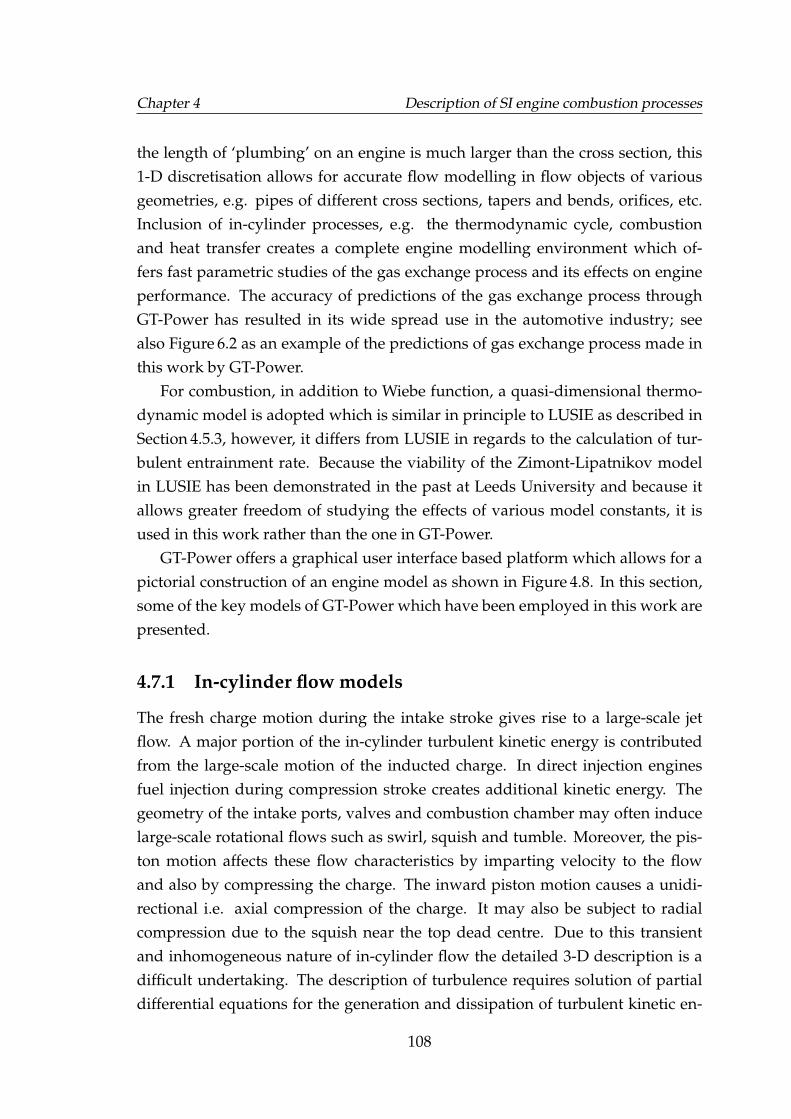
Chapter 4 Description of SI engine combustion processes
the length of ‘plumbing’ on an engine is much larger than the cross section, this1-D discretisation allows for accurate flow modelling in flow objects of variousgeometries, e.g. pipes of different cross sections, tapers and bends, orifices, etc.Inclusion of in-cylinder processes, e.g. the thermodynamic cycle, combustionand heat transfer creates a complete engine modelling environment which of-fers fast parametric studies of the gas exchange process and its effects on engineperformance. The accuracy of predictions of the gas exchange process throughGT-Power has resulted in its wide spread use in the automotive industry; seealso Figure 6.2 as an example of the predictions of gas exchange process made inthis work by GT-Power.
For combustion, in addition to Wiebe function, a quasi-dimensional thermo-dynamic model is adopted which is similar in principle to LUSIE as described inSection 4.5.3, however, it differs from LUSIE in regards to the calculation of tur-bulent entrainment rate. Because the viability of the Zimont-Lipatnikov modelin LUSIE has been demonstrated in the past at Leeds University and because itallows greater freedom of studying the effects of various model constants, it isused in this work rather than the one in GT-Power.
GT-Power offers a graphical user interface based platform which allows for apictorial construction of an engine model as shown in Figure 4.8. In this section,some of the key models of GT-Power which have been employed in this work arepresented.
4.7.1 In-cylinder flow models
The fresh charge motion during the intake stroke gives rise to a large-scale jetflow. A major portion of the in-cylinder turbulent kinetic energy is contributedfrom the large-scale motion of the inducted charge. In direct injection enginesfuel injection during compression stroke creates additional kinetic energy. Thegeometry of the intake ports, valves and combustion chamber may often inducelarge-scale rotational flows such as swirl, squish and tumble. Moreover, the pis-ton motion affects these flow characteristics by imparting velocity to the flowand also by compressing the charge. The inward piston motion causes a unidi-rectional i.e. axial compression of the charge. It may also be subject to radialcompression due to the squish near the top dead centre. Due to this transientand inhomogeneous nature of in-cylinder flow the detailed 3-D description is adifficult undertaking. The description of turbulence requires solution of partialdifferential equations for the generation and dissipation of turbulent kinetic en-
108
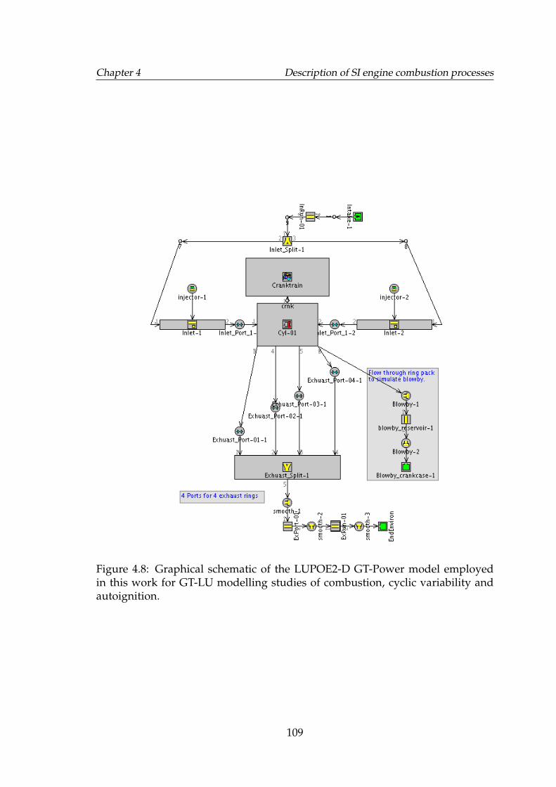
Chapter 4 Description of SI engine combustion processes
Figure 4.8: Graphical schematic of the LUPOE2-D GT-Power model employedin this work for GT-LU modelling studies of combustion, cyclic variability andautoignition.
109
Chapter 4 Description of SI engine combustion processes
IV
I II
III
I
Piston
Head
Cylinder
wall
Figure 4.9: Illustration showing the combustion chamber divided in four regionsfor each of which a pair of turbulent kinetic energy and dissipation rate equationsare solved.
ergy, e.g. as the widely used k − ε model. In computational fluid dynamics, thenumerical solution of the 3-D Navier-Stokes equations and turbulence equationsdiscretised over the whole cylinder volume is carried out. Such simulations aretime consuming and computationally expensive.
A much simpler alternative to CFD is a zonal approach as proposed by Moreland Mansour [1982] by means of which the state of turbulence is determined inrelatively larger regions or zones of the flow-field. In GT-Power, the combustionchamber is divided into four subvolumes as shown in Figure 4.9, in which theturbulence is assumed to be homogeneous and isotropic. The flow in each sub-volume is defined by the calculation of radial and axial velocities, swirl, squish,turbulence kinetic energy and a turbulent length scale. Details on this subvolumeapproach to the application of k − ε model in engines can be found in Morel andMansour [1982] and Morel and Keribar [1985].
4.7.1.1 Swirl, radial and axial velocities
The axial velocity component is determined from the piston kinematics which isthe velocity of the piston relative to the liner. The radial velocity is due to squishand the reverse squish between subvolume I and II (Figure 4.9). Squish occursas the piston reaches near the TDC and the subvolume I above the piston lipsqueezes out the charge mass radially inwards in the form of a turbulent jet. Theeffects of squish on turbulence depends on the geometry of the piston bowl andthe head but are generally weak. Squish intensifies the swirl but this happensfor only a short span of time and has negligible effect on the burn rate [Lumley,1999], however, it is accounted for in the model for swirl.
110
Chapter 4 Description of SI engine combustion processes
Swirl is determined by a model proposed in [Morel and Keribar, 1985] whichassumes that the flow in each subvolume revolves with a constant angular veloc-ity, magnitude of which is intensified as more mass enters the region either fromthe intake or a neighbouring region or it is reduced as the mass leaves. The angu-lar velocity of the swirl gradually decreases due to the viscous friction acting onthe surrounding walls.
4.7.1.2 Turbulence model
Morel and Mansour [1982] extended the standard k− ε model for engines follow-ing the proposition made by Reynolds [1980] on the limitations of the standardenergy dissipation equation to capture the behaviour of homogeneous turbulencein engines. Morel pointed out that in addition to Reynolds proposition of a spher-ical compression in engines, the compression is axial as well as radial. Use of orig-inal model was found to produce an unrealistic increase in the turbulent lengthscale as the charge was compressed. This problem was eliminated by modifyingthe kinetic energy production term by defining the local strain-rate tensor for thethree types of compressions i.e. pure spherical, axial and radial. The resultingtransport equations are presented here for reference. For kinetic energy:
(mjkj)′ =∑
mijkij +∑
ρUdiff (ki − kj)A+mjSk + mintk∗int − mexhk
∗exh
+minjk∗∗inj + msqk
∗∗sq
(4.38)
and for energy dissipation:
(mjεj)′ =∑
mijεij +∑
ρUdiff (εi − εj)A+mjSε + mintε∗int − mexhε
∗exh
+minjε∗∗inj + msqε
∗∗sq +
k2j
L2j
(4.39)
Where the superscript * indicates that the terms be applied to region I and IVand ** applies to region II, III and IV only. The subscript j refers to the regionunder consideration, i refers to the adjacent region. Subscript ij refers to thesituations where the subscript can either be i or j depending on the direction offlow between the two regions. Various kinetic energy source terms are: kint, dueto the charge inducted through the intake; kexh, due to the mass leaving to theexhaust; kinj , due to the fuel injection; ksq, due to squish. Further details on those
111
Chapter 4 Description of SI engine combustion processes
can be found in [Morel and Mansour, 1982].The two k − ε coupled partial differential equations are solved for all four
regions along with the equations for swirl and squish. The quasi-dimensionalmodelling of combustion results in a division of the charge in two zones, a burnedand an unburned zone. An assumption of a spherical flame which is truncatedby the chamber walls and the knowledge of the amount of mass burned helpsin determining the size and shape of the burned zone. The solution of the k − εmodel for all four regions results in the knowledge of total kinetic energy of eachregion which can then be used to determine specific kinetic energy of the burnedand unburned zone.
4.8 Introduction to GT-LU
GT-LU, which is formed by the coupling of GT-Power and LUSIE was first de-veloped by Hattrell [2007]. The description of the earlier version can be foundin [Hattrell et al., 2006]. For the current version of GT-LU, the relevant modelsof LUSIE were migrated to the newer user-templates of GT-Power v 7.2 and v 7.3with necessary restructuring of the subroutines to allow efficient simulation ofmultiple cases for multicylinder engines with cyclic variability and autoignitionmodelling. Some of the new modifications to GT-LU are listed below:
• In the older version, an empirical expression for the determination of u′ wasincorporated which correlated u′ to the mean piston speed. In the currentversion, for the in-cylinder flow description, provision has been made toeither employ the models available in GT-Power for swirl, tumble and thek − ε model for turbulence or to input spatially averaged u′ and L obtainedby CFD modelling of cold flow i.e. without combustion.
• The autoignition subroutine comprising of the previous empirical and skele-tal models of LUSIE have been retained while the newly developed chemi-cal kinetics solver has been added to GT-LU.
• Subroutines to model cyclic variability in combustion by using the approachoutlined in Section 4.6.6 were retained with appropriate restructuring in thecurrent version of GT-LU.
The operation of GT-LU is such that GT-Power controls the overall executionof the code and provides the user with the graphical user interface. The engine
112
Chapter 4 Description of SI engine combustion processes
model is constructed by the selection of appropriate submodels for engine geom-etry, fluid flow, heat transfer, combustion etc; an example of which is presentedin Figure 4.8. Figure 4.10 shows a flowchart of sequence of operations carried outby GT-LU. Details on the use of GT-LU can be found in AppendixA.1.
4.9 CFD modelling of turbulence
The multi-zone approach to combustion modelling abandons the geometric de-tails of the flow-field i.e. it assumes homogeneous and isotropic turbulence. Toaccompany this approach the nature of in-cylinder flow is simplified and de-scribed by quantities such as u′ and L obtained after averaging. Intensive anddetailed CFD modelling approaches such as Direct Numerical Simulation (DNS)and even the relatively simplified approaches such as Large Eddy Simulation(LES) and the solution of Reynolds Averaged Navier-Stokes (RANS) equationsare not justifiable when a multi-zone combustion model is to be used as the su-perfluity of 3-D details of the flow are to be eventually averaged into a single rep-resentative quantity for the whole volume. Moreover, the computational powerand time required for such simulations are of the order of a few days to weeks.The k − ε turbulence model makes an a priori assumption that the turbulence isisotropic and therefore the turbulence intensity and length scales can be taken asscalars. This major simplification of the k − ε model results in its ease of use anddue to which it is widely popular. Its implementation in a simpler domain (sub-volume approach as discussed in Section 4.7.1.2) has also seen great use. How-ever, typically during the engine development process, CFD modelling of theflow from the intake runners, through the ports and into the cylinder is carriedout to optimise geometries for better bulk flow characteristics such as swirl andtumble. Normally, revised k−εmodels are used such as the RNG k−εmodel; i.e.obtained by using the Re-Normalisation Group methods. This model was used insupport of this work. From such simulations, the mass averaged kinetic energyof the charge can be obtained as well as an integral length scale and can be usedfor multi-zone combustion modelling. It is of interest to compare the turbulencecalculations of the subvolume approach to the k − ε model in GT-Power and theCFD modelling results from a RNG k− ε model. This comparison is presented inChapter 6.
The CFD modelling in support of this work was carried out with the package,Star-CD, at Mahle Powetrain Ltd. The kinetic energy averaged over the whole
113
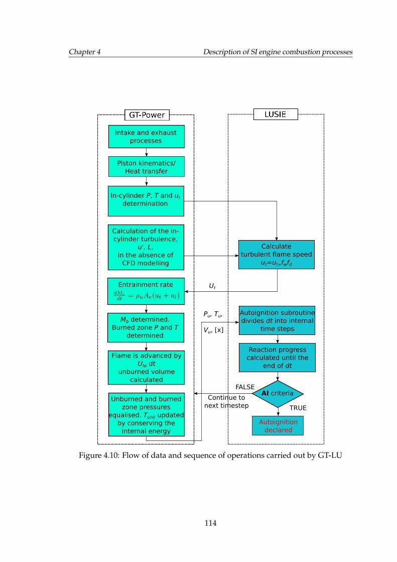
Chapter 4 Description of SI engine combustion processes
Intake and exhaust
processes
Piston kinematics/
Heat transfer
In-cylinder P, T and ul
determination
Calculate
turbulent flame speed
ut=ut∞fwfd
Calculation of the in-
cylinder turbulence,
u', L,
in the absence of
CFD modelling
Entrainment rate
Mb determined.
Burned zone P and T
determined
Flame is advanced by
Ute dt
unburned volume
calculated
Unburned and burned
zone pressures
equalised. Tunb updated
by conserving the
internal energy
Autoignition subroutine
divides dt into internal
time steps
Reaction progress
calculated until the
end of dt
AI criteria
TRUE
FALSE
Autoignition
declared
Pu, Tu,
Vu, [x]
Continue to
next timestep
Ut
Figure 4.10: Flow of data and sequence of operations carried out by GT-LU
114
Chapter 4 Description of SI engine combustion processes
cylinder charge for cold flow, i.e. without combustion, and is used as an inputto the entrainment model. This makes the turbulence generated from CFD dif-ferent from the subvolume approach in which only the unburned mass is usedin the averaging. The subvolume approach tends to over predict the turbulenceintensity because of large sized subvolumes on which the transport equations areapplied. Mass transfer between these subvolumes is accounted for in the bulkflow whereas the motion of the mass which stays with in one region constitutesturbulence.
4.10 Description of the test cases
No experimental work was undertaken by the author, however, the modellingwork has been supported by measurements from two research engines. One,LUPOE2-D which is a bespoke optical research engine at the University of Leedsand the second engine, a 3-cylinder downsized, technology demonstrator enginedesigned and built at Mahle Powertrain Ltd. It is referred here as the Mahle Di3engine. The description of these engines is given in following sections.
4.10.1 LUPOE2-D
LUPOE is the acronym for Leeds University Ported Optical Engine constructedon top of a single cylinder agricultural diesel engine made by Lister-Petter whichdonated the crank assembly on which bespoke piston, head and liner were in-stalled. Modifications were also made to the intake and exhaust system. Thename LUPOE is followed by a number indicating the generation and an alphabetwhich indicates the combustion chamber or head geometry; such as LUPOE2-D, which has a disk shaped combustion chamber i.e. a flat head and piston.LUPOE2-D experiments performed by Roberts [2010] have been analysed in thiswork and used in support of the combustion and autoignition modelling. The ex-perimental setup is shown in Figure 4.12 and the design specifications of LUPOE2-D are presented in Table 4.1.
Modifications to the intake and exhaust system were made with the inten-tion to reduce large-scale mean flow as much as possible. This was attemptedby orienting the two diametrically opposed intake ports at a certain angle to thecylinder axis that minimal bulk flow motion is achieved in the cylinder (see Fig-ure 4.11). The liner was designed to have four staggered rings of exhaust ports as
115
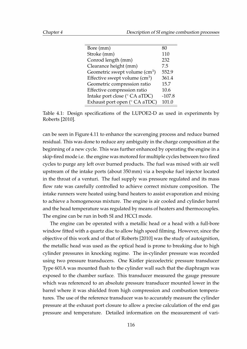
Chapter 4 Description of SI engine combustion processes
Bore (mm) 80Stroke (mm) 110Conrod length (mm) 232Clearance height (mm) 7.5Geometric swept volume (cm3) 552.9Effective swept volume (cm3) 361.4Geometric compression ratio 15.7Effective compression ratio 10.6Intake port close (◦ CA aTDC) -107.8Exhaust port open (◦ CA aTDC) 101.0
Table 4.1: Design specifications of the LUPOE2-D as used in experiments byRoberts [2010].
can be seen in Figure 4.11 to enhance the scavenging process and reduce burnedresidual. This was done to reduce any ambiguity in the charge composition at thebeginning of a new cycle. This was further enhanced by operating the engine in askip-fired mode i.e. the engine was motored for multiple cycles between two firedcycles to purge any left over burned products. The fuel was mixed with air wellupstream of the intake ports (about 350 mm) via a bespoke fuel injector locatedin the throat of a venturi. The fuel supply was pressure regulated and its massflow rate was carefully controlled to achieve correct mixture composition. Theintake runners were heated using band heaters to assist evaporation and mixingto achieve a homogeneous mixture. The engine is air cooled and cylinder barreland the head temperature was regulated by means of heaters and thermocouples.The engine can be run in both SI and HCCI mode.
The engine can be operated with a metallic head or a head with a full-borewindow fitted with a quartz disc to allow high speed filming. However, since theobjective of this work and of that of Roberts [2010] was the study of autoignition,the metallic head was used as the optical head is prone to breaking due to highcylinder pressures in knocking regime. The in-cylinder pressure was recordedusing two pressure transducers. One Kistler piezoelectric pressure transducerType 601A was mounted flush to the cylinder wall such that the diaphragm wasexposed to the chamber surface. This transducer measured the gauge pressurewhich was referenced to an absolute pressure transducer mounted lower in thebarrel where it was shielded from high compression and combustion tempera-tures. The use of the reference transducer was to accurately measure the cylinderpressure at the exhaust port closure to allow a precise calculation of the end gaspressure and temperature. Detailed information on the measurement of vari-
116
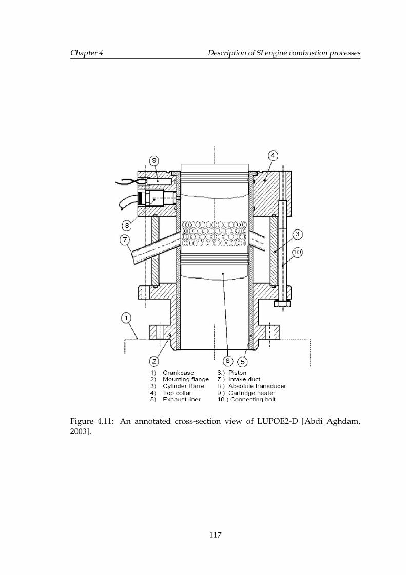
Chapter 4 Description of SI engine combustion processes
Figure 4.11: An annotated cross-section view of LUPOE2-D [Abdi Aghdam,2003].
117
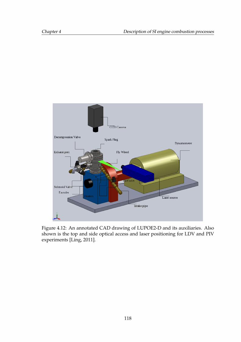
Chapter 4 Description of SI engine combustion processes
Figure 4.12: An annotated CAD drawing of LUPOE2-D and its auxiliaries. Alsoshown is the top and side optical access and laser positioning for LDV and PIVexperiments [Ling, 2011].
118
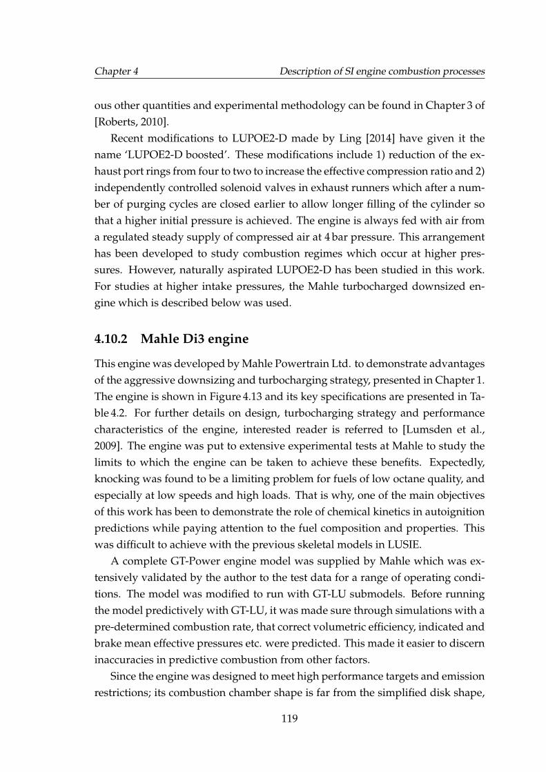
Chapter 4 Description of SI engine combustion processes
ous other quantities and experimental methodology can be found in Chapter 3 of[Roberts, 2010].
Recent modifications to LUPOE2-D made by Ling [2014] have given it thename ‘LUPOE2-D boosted’. These modifications include 1) reduction of the ex-haust port rings from four to two to increase the effective compression ratio and 2)independently controlled solenoid valves in exhaust runners which after a num-ber of purging cycles are closed earlier to allow longer filling of the cylinder sothat a higher initial pressure is achieved. The engine is always fed with air froma regulated steady supply of compressed air at 4 bar pressure. This arrangementhas been developed to study combustion regimes which occur at higher pres-sures. However, naturally aspirated LUPOE2-D has been studied in this work.For studies at higher intake pressures, the Mahle turbocharged downsized en-gine which is described below was used.
4.10.2 Mahle Di3 engine
This engine was developed by Mahle Powertrain Ltd. to demonstrate advantagesof the aggressive downsizing and turbocharging strategy, presented in Chapter 1.The engine is shown in Figure 4.13 and its key specifications are presented in Ta-ble 4.2. For further details on design, turbocharging strategy and performancecharacteristics of the engine, interested reader is referred to [Lumsden et al.,2009]. The engine was put to extensive experimental tests at Mahle to study thelimits to which the engine can be taken to achieve these benefits. Expectedly,knocking was found to be a limiting problem for fuels of low octane quality, andespecially at low speeds and high loads. That is why, one of the main objectivesof this work has been to demonstrate the role of chemical kinetics in autoignitionpredictions while paying attention to the fuel composition and properties. Thiswas difficult to achieve with the previous skeletal models in LUSIE.
A complete GT-Power engine model was supplied by Mahle which was ex-tensively validated by the author to the test data for a range of operating condi-tions. The model was modified to run with GT-LU submodels. Before runningthe model predictively with GT-LU, it was made sure through simulations with apre-determined combustion rate, that correct volumetric efficiency, indicated andbrake mean effective pressures etc. were predicted. This made it easier to discerninaccuracies in predictive combustion from other factors.
Since the engine was designed to meet high performance targets and emissionrestrictions; its combustion chamber shape is far from the simplified disk shape,
119
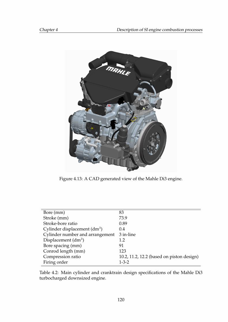
Chapter 4 Description of SI engine combustion processes
Figure 4.13: A CAD generated view of the Mahle Di3 engine.
Bore (mm) 83Stroke (mm) 73.9Stroke-bore ratio 0.89Cylinder displacement (dm3) 0.4Cylinder number and arrangement 3 in-lineDisplacement (dm3) 1.2Bore spacing (mm) 91Conrod length (mm) 123Compression ratio 10.2, 11.2, 12.2 (based on piston design)Firing order 1-3-2
Table 4.2: Main cylinder and cranktrain design specifications of the Mahle Di3turbocharged downsized engine.
120
Chapter 4 Description of SI engine combustion processes
Figure 4.14: Views of the cylinder head (left) and the piston crown (right) of theMahle Di3 engine.
it is shown in Figure 4.14. Owing to the complex shape of the head and more soof the piston crown, determining the recess volumes to be used for turbulencecalculations in GT-Power was not so straightforward. However, volumes weredetermined by means of a CAD software (SolidWorks) and necessary approxi-mations were made where determining subvolumes directly was not possible.
121
Chapter 5
Autoignition in LUPOE2-D
5.1 Introduction
Numerous studies have demonstrated that autoignition in HCCI and controlledautoignition (CAI) engines can be reliably predicted using multi-component gaso-line surrogate mechanisms, e.g. [Andrae and Head, 2009; Knop et al., 2013].However, autoignition occurs in HCCI and CAI engines at in-cylinder pressuresand temperatures typically much lower than in an SI engine, especially if thelatter is supercharged. Furthermore, as stated earlier, chemical kinetic mecha-nisms are routinely validated against shock tube and rapid compression machinemeasurements of the ignition delay times, τign, of various gasoline surrogate fu-els. The conditions for these laboratory measurements are similar to those whichprevail before ignition in an HCCI or CAI engine, and the recent kinetic mech-anisms, e.g. Andrae and Head [2009]; Huang et al. [2010]; Ra and Reitz [2011],perform remarkably well at these regimes as shown in various Arrhenius plotsin Chapter 2, e.g. Figures 2.10 and 2.11. Yet, in an SI engine the propagating pre-mixed flame induces higher end gas pressure and temperature and the questionarises of whether the reduced chemical mechanism will perform equally well.This Chapter covers the application of the three reduced chemical kinetic mecha-nisms studied in Chapters 2 & 3, to the prediction of autoignition in LUPOE2-D.
A review of practical gasoline surrogates was presented in Section 2.8 and theapproaches to gasoline surrogate selection were presented in Section 2.9. In thisChapter these approaches have been employed to formulate surrogates to model
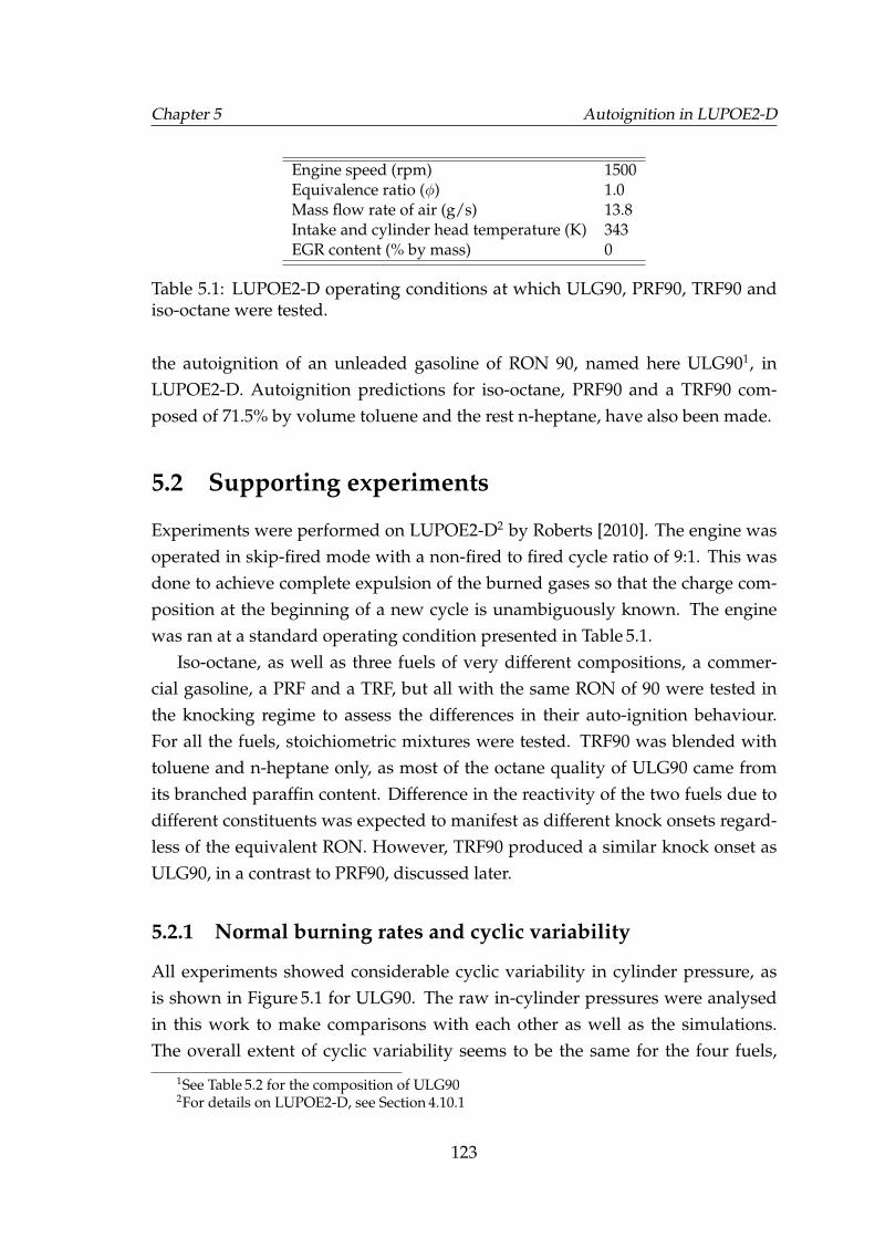
Chapter 5 Autoignition in LUPOE2-D
Engine speed (rpm) 1500Equivalence ratio (φ) 1.0Mass flow rate of air (g/s) 13.8Intake and cylinder head temperature (K) 343EGR content (% by mass) 0
Table 5.1: LUPOE2-D operating conditions at which ULG90, PRF90, TRF90 andiso-octane were tested.
the autoignition of an unleaded gasoline of RON 90, named here ULG901, inLUPOE2-D. Autoignition predictions for iso-octane, PRF90 and a TRF90 com-posed of 71.5% by volume toluene and the rest n-heptane, have also been made.
5.2 Supporting experiments
Experiments were performed on LUPOE2-D2 by Roberts [2010]. The engine wasoperated in skip-fired mode with a non-fired to fired cycle ratio of 9:1. This wasdone to achieve complete expulsion of the burned gases so that the charge com-position at the beginning of a new cycle is unambiguously known. The enginewas ran at a standard operating condition presented in Table 5.1.
Iso-octane, as well as three fuels of very different compositions, a commer-cial gasoline, a PRF and a TRF, but all with the same RON of 90 were tested inthe knocking regime to assess the differences in their auto-ignition behaviour.For all the fuels, stoichiometric mixtures were tested. TRF90 was blended withtoluene and n-heptane only, as most of the octane quality of ULG90 came fromits branched paraffin content. Difference in the reactivity of the two fuels due todifferent constituents was expected to manifest as different knock onsets regard-less of the equivalent RON. However, TRF90 produced a similar knock onset asULG90, in a contrast to PRF90, discussed later.
5.2.1 Normal burning rates and cyclic variability
All experiments showed considerable cyclic variability in cylinder pressure, asis shown in Figure 5.1 for ULG90. The raw in-cylinder pressures were analysedin this work to make comparisons with each other as well as the simulations.The overall extent of cyclic variability seems to be the same for the four fuels,
1See Table 5.2 for the composition of ULG902For details on LUPOE2-D, see Section 4.10.1
123
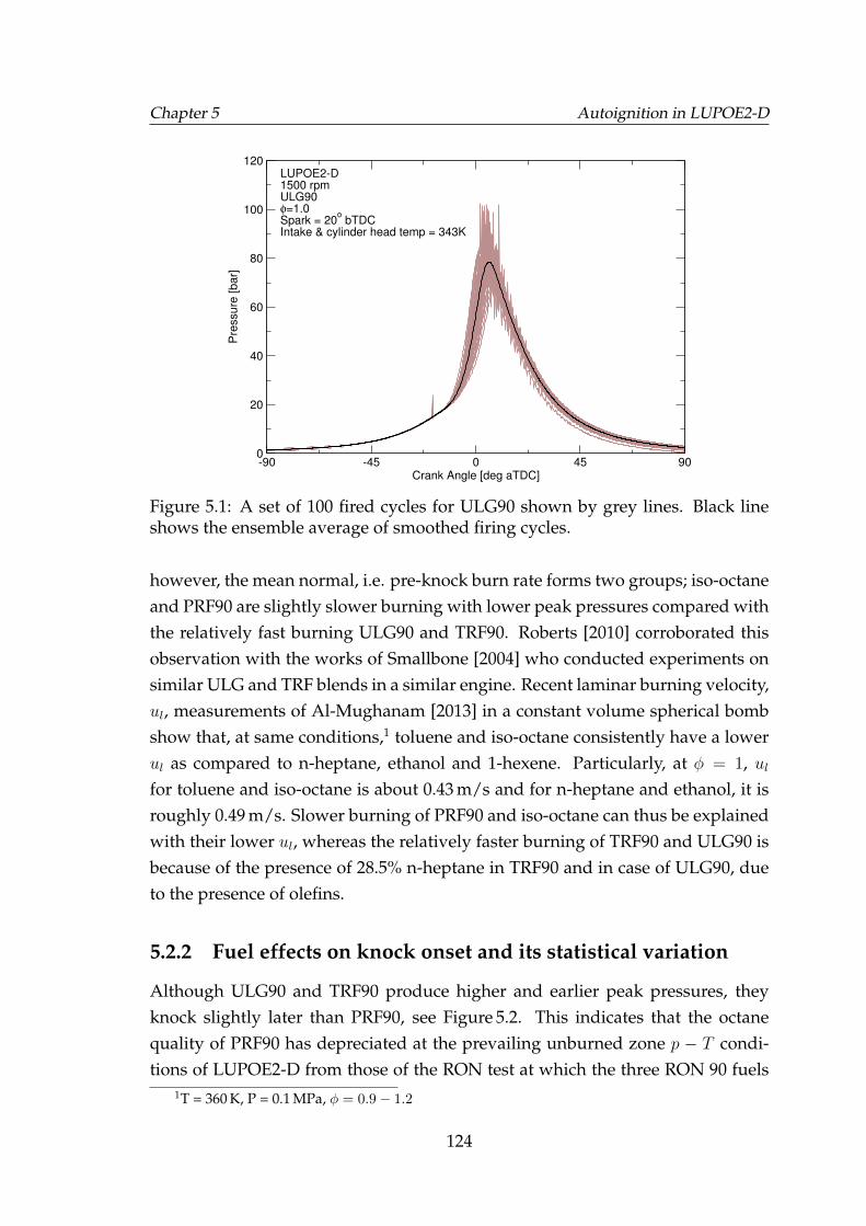
Chapter 5 Autoignition in LUPOE2-D
-90 -45 0 45 90Crank Angle [deg aTDC]
0
20
40
60
80
100
120
Pre
ssu
re [
ba
r]
LUPOE2-D1500 rpmULG90φ=1.0Spark = 20
o bTDC
Intake & cylinder head temp = 343K
Figure 5.1: A set of 100 fired cycles for ULG90 shown by grey lines. Black lineshows the ensemble average of smoothed firing cycles.
however, the mean normal, i.e. pre-knock burn rate forms two groups; iso-octaneand PRF90 are slightly slower burning with lower peak pressures compared withthe relatively fast burning ULG90 and TRF90. Roberts [2010] corroborated thisobservation with the works of Smallbone [2004] who conducted experiments onsimilar ULG and TRF blends in a similar engine. Recent laminar burning velocity,ul, measurements of Al-Mughanam [2013] in a constant volume spherical bombshow that, at same conditions,1 toluene and iso-octane consistently have a lowerul as compared to n-heptane, ethanol and 1-hexene. Particularly, at φ = 1, ulfor toluene and iso-octane is about 0.43 m/s and for n-heptane and ethanol, it isroughly 0.49 m/s. Slower burning of PRF90 and iso-octane can thus be explainedwith their lower ul, whereas the relatively faster burning of TRF90 and ULG90 isbecause of the presence of 28.5% n-heptane in TRF90 and in case of ULG90, dueto the presence of olefins.
5.2.2 Fuel effects on knock onset and its statistical variation
Although ULG90 and TRF90 produce higher and earlier peak pressures, theyknock slightly later than PRF90, see Figure 5.2. This indicates that the octanequality of PRF90 has depreciated at the prevailing unburned zone p − T condi-tions of LUPOE2-D from those of the RON test at which the three RON 90 fuels
1T = 360 K, P = 0.1 MPa, φ = 0.9− 1.2
124
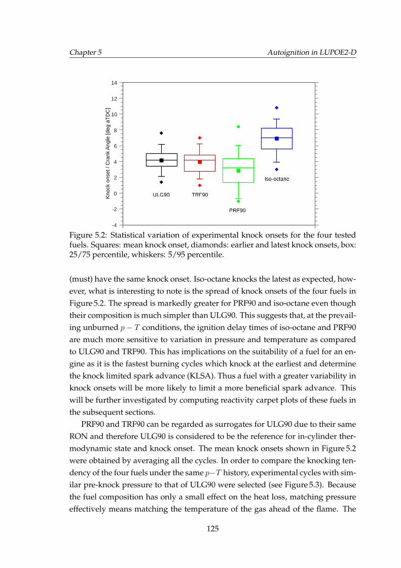
Chapter 5 Autoignition in LUPOE2-D
Knock o
nset / Cra
nk A
ngle
[deg a
TDC]
4
2
0
2
4
6
8
10
12
14
Figure 5.2: Statistical variation of experimental knock onsets for the four testedfuels. Squares: mean knock onset, diamonds: earlier and latest knock onsets, box:25/75 percentile, whiskers: 5/95 percentile.
(must) have the same knock onset. Iso-octane knocks the latest as expected, how-ever, what is interesting to note is the spread of knock onsets of the four fuels inFigure 5.2. The spread is markedly greater for PRF90 and iso-octane even thoughtheir composition is much simpler than ULG90. This suggests that, at the prevail-ing unburned p− T conditions, the ignition delay times of iso-octane and PRF90are much more sensitive to variation in pressure and temperature as comparedto ULG90 and TRF90. This has implications on the suitability of a fuel for an en-gine as it is the fastest burning cycles which knock at the earliest and determinethe knock limited spark advance (KLSA). Thus a fuel with a greater variability inknock onsets will be more likely to limit a more beneficial spark advance. Thiswill be further investigated by computing reactivity carpet plots of these fuels inthe subsequent sections.
PRF90 and TRF90 can be regarded as surrogates for ULG90 due to their sameRON and therefore ULG90 is considered to be the reference for in-cylinder ther-modynamic state and knock onset. The mean knock onsets shown in Figure 5.2were obtained by averaging all the cycles. In order to compare the knocking ten-dency of the four fuels under the same p−T history, experimental cycles with sim-ilar pre-knock pressure to that of ULG90 were selected (see Figure 5.3). Becausethe fuel composition has only a small effect on the heat loss, matching pressureeffectively means matching the temperature of the gas ahead of the flame. The
125
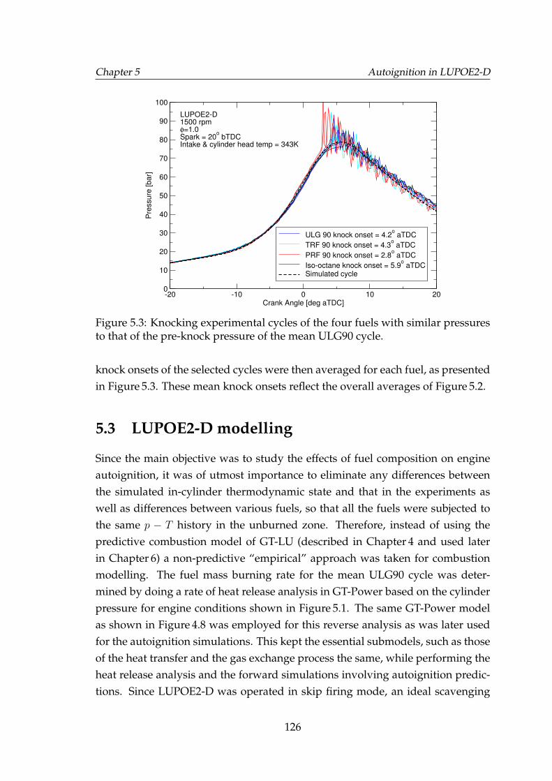
Chapter 5 Autoignition in LUPOE2-D
-20 -10 0 10 20Crank Angle [deg aTDC]
0
10
20
30
40
50
60
70
80
90
100
Pre
ssu
re [
ba
r]
ULG 90 knock onset = 4.2o aTDC
TRF 90 knock onset = 4.3o aTDC
PRF 90 knock onset = 2.8o aTDC
Iso-octane knock onset = 5.9o aTDC
Simulated cycle
LUPOE2-D1500 rpmφ=1.0Spark = 20
o bTDC
Intake & cylinder head temp = 343K
Figure 5.3: Knocking experimental cycles of the four fuels with similar pressuresto that of the pre-knock pressure of the mean ULG90 cycle.
knock onsets of the selected cycles were then averaged for each fuel, as presentedin Figure 5.3. These mean knock onsets reflect the overall averages of Figure 5.2.
5.3 LUPOE2-D modelling
Since the main objective was to study the effects of fuel composition on engineautoignition, it was of utmost importance to eliminate any differences betweenthe simulated in-cylinder thermodynamic state and that in the experiments aswell as differences between various fuels, so that all the fuels were subjected tothe same p − T history in the unburned zone. Therefore, instead of using thepredictive combustion model of GT-LU (described in Chapter 4 and used laterin Chapter 6) a non-predictive “empirical” approach was taken for combustionmodelling. The fuel mass burning rate for the mean ULG90 cycle was deter-mined by doing a rate of heat release analysis in GT-Power based on the cylinderpressure for engine conditions shown in Figure 5.1. The same GT-Power modelas shown in Figure 4.8 was employed for this reverse analysis as was later usedfor the autoignition simulations. This kept the essential submodels, such as thoseof the heat transfer and the gas exchange process the same, while performing theheat release analysis and the forward simulations involving autoignition predic-tions. Since LUPOE2-D was operated in skip firing mode, an ideal scavenging
126
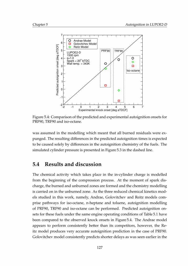
Chapter 5 Autoignition in LUPOE2-D
-2 -1 0 1 2 3 4 5 6 7Experimental knock onset [deg aTDCF]
-2
-1
0
1
2
3
4
5
6
7
Pre
dic
ted a
uto
ignitio
n o
nset [d
eg a
TD
CF
]
Andrae ModelGolovitchev ModelReitz Model
PRF90 TRF90
Iso-octane
LUPOE2-D1500 rpmφ=1.0Spark = 20
o bTDC
Wall temp. = 343K
Figure 5.4: Comparison of the predicted and experimental autoignition onsets forPRF90, TRF90 and iso-octane.
was assumed in the modelling which meant that all burned residuals were ex-punged. The resulting differences in the predicted autoignition times is expectedto be caused solely by differences in the autoignition chemistry of the fuels. Thesimulated cylinder pressure is presented in Figure 5.3 in the dashed line.
5.4 Results and discussion
The chemical activity which takes place in the in-cylinder charge is modelledfrom the beginning of the compression process. At the moment of spark dis-charge, the burned and unburned zones are formed and the chemistry modellingis carried on in the unburned zone. As the three reduced chemical kinetics mod-els studied in this work, namely, Andrae, Golovitchev and Reitz models com-prise pathways for iso-octane, n-heptane and toluene, autoignition modellingof PRF90, TRF90 and iso-octane can be performed. Predicted autoignition on-sets for these fuels under the same engine operating conditions of Table 5.1 havebeen compared to the observed knock onsets in Figure 5.4. The Andrae modelappears to perform consistently better than its competitors, however, the Re-itz model produces very accurate autoignition prediction in the case of PRF90.Golovitchev model consistently predicts shorter delays as was seen earlier in the
127
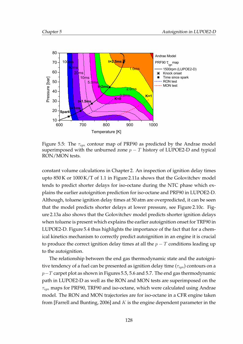
Chapter 5 Autoignition in LUPOE2-D
100ms50ms
20ms10ms
5.0ms
3.0ms
2.0ms
1.0ms
600 700 800 900 100010
20
30
40
50
60
70
80
t=1ms
K=1K=0
t=2.5ms
t=2ms
1500rpm (LUPOE2-D) Knock onset Time since spark RON test MON test
Temperature [K]
Pres
sure
[bar
]
Andrae Model
PRF90ign
map
Spark
t=1.5ms
Figure 5.5: The τign contour map of PRF90 as predicted by the Andrae modelsuperimposed with the unburned zone p − T history of LUPOE2-D and typicalRON/MON tests.
constant volume calculations in Chapter 2. An inspection of ignition delay timesupto 850 K or 1000 K/T of 1.1 in Figure 2.11a shows that the Golovitchev modeltends to predict shorter delays for iso-octane during the NTC phase which ex-plains the earlier autoignition prediction for iso-octane and PRF90 in LUPOE2-D.Although, toluene ignition delay times at 50 atm are overpredicted, it can be seenthat the model predicts shorter delays at lower pressure, see Figure 2.10c. Fig-ure 2.13a also shows that the Golovitchev model predicts shorter ignition delayswhen toluene is present which explains the earlier autoignition onset for TRF90 inLUPOE2-D. Figure 5.4 thus highlights the importance of the fact that for a chem-ical kinetics mechanism to correctly predict autoignition in an engine it is crucialto produce the correct ignition delay times at all the p− T conditions leading upto the autoignition.
The relationship between the end gas thermodynamic state and the autoigni-tive tendency of a fuel can be presented as ignition delay time (τign) contours on ap−T carpet plot as shown in Figures 5.5, 5.6 and 5.7. The end gas thermodynamicpath in LUPOE2-D as well as the RON and MON tests are superimposed on theτign maps for PRF90, TRF90 and iso-octane, which were calculated using Andraemodel. The RON and MON trajectories are for iso-octane in a CFR engine takenfrom [Farrell and Bunting, 2006] and K is the engine dependent parameter in the
128
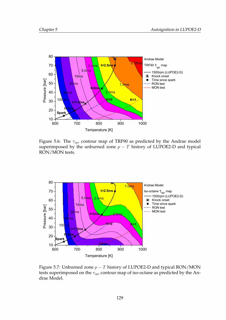
Chapter 5 Autoignition in LUPOE2-D
100ms
50ms
20ms
10ms5.0ms
3.0ms
2.0ms
1.0ms
0.50ms
600 700 800 900 100010
20
30
40
50
60
70
80
t=1.5msK=0 K=1
t=2.5ms
t=2ms
t=1ms
1500rpm (LUPOE2-D) Knock onset Time since spark RON test MON test
Temperature [K]
Pres
sure
[bar
]
Andrae Model
TRF90 ign
map
Spark
Figure 5.6: The τign contour map of TRF90 as predicted by the Andrae modelsuperimposed by the unburned zone p − T history of LUPOE2-D and typicalRON/MON tests.
100ms
50ms
20ms
10ms
5.0ms
3.0ms
2.0ms
1.0ms
50ms600 700 800 900 1000
10
20
30
40
50
60
70
80
t=1.5msK=1K=0
t=2.5ms
t=2ms
t=1ms
1500rpm (LUPOE2-D) Knock onset Time since spark RON test MON test
Temperature [K]
Pres
sure
[bar
]
Spark
Andrae Model
Iso-octane ign map
Figure 5.7: Unburned zone p − T history of LUPOE2-D and typical RON/MONtests superimposed on the τign contour map of iso-octane as predicted by the An-drae Model.
129
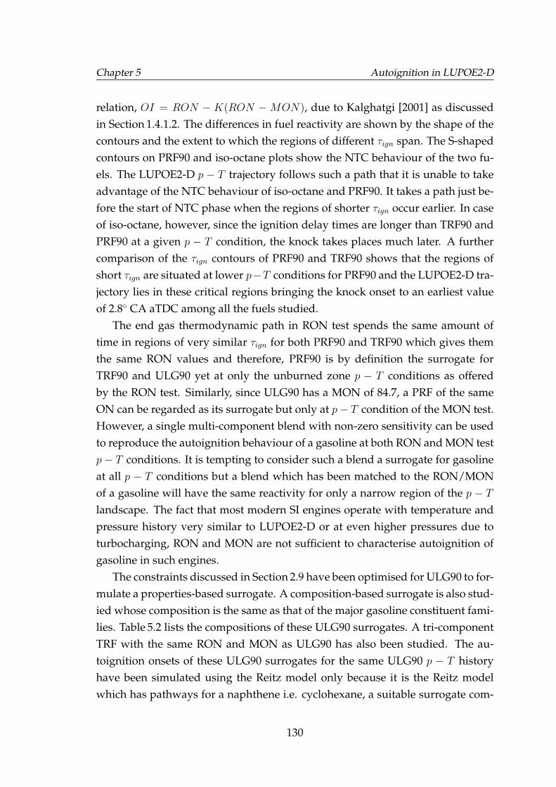
Chapter 5 Autoignition in LUPOE2-D
relation, OI = RON − K(RON −MON), due to Kalghatgi [2001] as discussedin Section 1.4.1.2. The differences in fuel reactivity are shown by the shape of thecontours and the extent to which the regions of different τign span. The S-shapedcontours on PRF90 and iso-octane plots show the NTC behaviour of the two fu-els. The LUPOE2-D p − T trajectory follows such a path that it is unable to takeadvantage of the NTC behaviour of iso-octane and PRF90. It takes a path just be-fore the start of NTC phase when the regions of shorter τign occur earlier. In caseof iso-octane, however, since the ignition delay times are longer than TRF90 andPRF90 at a given p − T condition, the knock takes places much later. A furthercomparison of the τign contours of PRF90 and TRF90 shows that the regions ofshort τign are situated at lower p−T conditions for PRF90 and the LUPOE2-D tra-jectory lies in these critical regions bringing the knock onset to an earliest valueof 2.8◦ CA aTDC among all the fuels studied.
The end gas thermodynamic path in RON test spends the same amount oftime in regions of very similar τign for both PRF90 and TRF90 which gives themthe same RON values and therefore, PRF90 is by definition the surrogate forTRF90 and ULG90 yet at only the unburned zone p − T conditions as offeredby the RON test. Similarly, since ULG90 has a MON of 84.7, a PRF of the sameON can be regarded as its surrogate but only at p− T condition of the MON test.However, a single multi-component blend with non-zero sensitivity can be usedto reproduce the autoignition behaviour of a gasoline at both RON and MON testp− T conditions. It is tempting to consider such a blend a surrogate for gasolineat all p − T conditions but a blend which has been matched to the RON/MONof a gasoline will have the same reactivity for only a narrow region of the p − Tlandscape. The fact that most modern SI engines operate with temperature andpressure history very similar to LUPOE2-D or at even higher pressures due toturbocharging, RON and MON are not sufficient to characterise autoignition ofgasoline in such engines.
The constraints discussed in Section 2.9 have been optimised for ULG90 to for-mulate a properties-based surrogate. A composition-based surrogate is also stud-ied whose composition is the same as that of the major gasoline constituent fami-lies. Table 5.2 lists the compositions of these ULG90 surrogates. A tri-componentTRF with the same RON and MON as ULG90 has also been studied. The au-toignition onsets of these ULG90 surrogates for the same ULG90 p − T historyhave been simulated using the Reitz model only because it is the Reitz modelwhich has pathways for a naphthene i.e. cyclohexane, a suitable surrogate com-
130
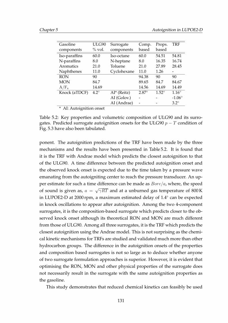
Chapter 5 Autoignition in LUPOE2-D
Gasoline ULG90 Surrogate Comp. Props. TRFcomponents % vol. components based basedIso-paraffins 60.0 Iso-octane 60.0 54.51 54.81N-paraffins 8.0 N-heptane 8.0 16.35 16.74Aromatics 21.0 Toluene 21.0 27.89 28.45Naphthenes 11.0 Cyclohexane 11.0 1.26 -RON 90 94.38 90 90MON 84.7 89.65 84.7 84.67A/Fs 14.69 14.56 14.69 14.49Knock (aTDCF) 4.2◦ AI* (Reitz) 2.87◦ 1.52◦ 1.16◦
AI (Golov.) - - -1.06◦
AI (Andrae) - - 3.2◦
* AI: Autoignition onset
Table 5.2: Key properties and volumetric composition of ULG90 and its surro-gates. Predicted surrogate autoignition onsets for the ULG90 p − T condition ofFig. 5.3 have also been tabulated.
ponent. The autoignition predictions of the TRF have been made by the threemechanisms and the results have been presented in Table 5.2. It is found thatit is the TRF with Andrae model which predicts the closest autoignition to thatof the ULG90. A time difference between the predicted autoignition onset andthe observed knock onset is expected due to the time taken by a pressure waveemanating from the autoigniting center to reach the pressure transducer. An up-per estimate for such a time difference can be made as Bore/a, where, the speedof sound is given as, a =
√γRT and at a unburned gas temperature of 800 K
in LUPOE2-D at 2000 rpm, a maximum estimated delay of 1.4◦ can be expectedin knock oscillations to appear after autoignition. Among the two 4-componentsurrogates, it is the composition-based surrogate which predicts closer to the ob-served knock onset although its theoretical RON and MON are much differentfrom those of ULG90. Among all three surrogates, it is the TRF which predicts theclosest autoignition using the Andrae model. This is not surprising as the chemi-cal kinetic mechanisms for TRFs are studied and validated much more than otherhydrocarbon groups. The difference in the autoignition onsets of the propertiesand composition based surrogates is not so large as to deduce whether anyoneof two surrogate formulation approaches is superior. However, it is evident thatoptimising the RON, MON and other physical properties of the surrogate doesnot necessarily result in the surrogate with the same autoignition properties asthe gasoline.
This study demonstrates that reduced chemical kinetics can feasibly be used
131
Chapter 5 Autoignition in LUPOE2-D
in the prediction of gasoline autoignition in an SI engine by approximating itsproperties by a surrogate. The choice of the mechanism and the surrogate af-fect greatly the prediction accuracy. The choice of the surrogate components ishowever limited by the availability of mechanisms for their oxidation. Surrogatecomposition may ideally be optimised by using target properties as constraints,however, weaknesses in the available empirical octane number models make thisapproach unreliable. Although the prediction of octane numbers is important inthe formulation of a surrogate but matching of the RON and MON does not guar-antee the correct reproduction of gasoline ignition behaviour in the surrogate asthe modern SI engines operate at conditions much different form the RON andMON tests. Moreover, a compositional fidelity of the surrogate to that of thegasoline is also important in producing the correct autoignition behaviour in thesurrogate.
The mechanisms generally over-predict the ignition delay time at low temper-atures and pressure of about 40 bar. However, earlier autoignition onsets in an en-gine have been predicted by the three models; in particular the Golovitchev andReitz models, indicating shorter ignition delay time predictions at lower pres-sures.
132
Chapter 6
Combustion and autoignitionmodelling in a turbocharged SIengine
6.1 Introduction
As the main objective of this project was to develop combustion and autoignitionmodelling tools and test their viability for a highly turbocharged downsized SIengine, the combustion, cyclic variability and chemical kinetics models discussedin Chapters 2 & 4 were used to model the Di31 engine at various operating con-ditions. Recent notable application of the LUSIE/GT-LU to engine modelling hasbeen done by Conway [2013] and Hattrell [2007]. Conway [2013] found throughhis modelling of six engines, both naturally aspirated and turbocharged, that thecombustion models were not capable of predicting combustion accurately for dif-ferent intake pressures. An adjustment of the turbulent length scale had to bemade through a multiplier in Equation 4.15 for the after-burning2 expressions inorder to achieve a good agreement with the experiments, however, this adjust-ment was kept to a minimum. It has been observed during the course of thiswork as well, that there is no single universal set of model constants for differentengines and different load and speed points of a given engine. Previously, mod-
1See Section 4.10.2 for the engine details.2See Section 4.5.3 for details on after-burning in a three-zone combustion model.
Chapter 6 Combustion and autoignition modelling in a turbocharged SI engine
elling studies of LUPOE with both disc-shaped and pent-roof combustion cham-bers, [Hattrell, 2007], were done with appreciable accuracy with a fixed set ofconstants mostly optimised from constant volume bomb experiments (e.g. [R. G.Abdel-Gayed and Bradley, 1984]) and LUPOE itself. But LUPOE has been lim-ited to low crankshaft speeds (up to 1500 rpm) and it has only recently been up-graded to operate at boosted pressures (up to 2 bar). At these conditions the com-bustion model in LUSIE/GT-LU performs fairly well, however, model predic-tions deviate from measurements for high load, high speed conditions of produc-tion engines; in many cases the latter use special intake arrangements to inducevery high turbulence, highly directional mean flow patterns and heavy pressurecharging. Effects of pressure charging on pre-mixed turbulent combustion is anon-going research interest and has also been studied in this work. Modelling ofcyclic variability in conjunction with chemical kinetics modelling of autoignitionhas been carried out to determine if this approach predicts a reasonable percent-age of knocking cycles and if this can be used to predict the knock limited sparkadvance (KLSA). The aims of studies presented in this Chapter are summarisedin the following:
• Assess combustion modelling for a variety of load-speed points.
• Compare the in-cylinder turbulence calculations of CFD modelling and thek − ε model of GT-Power for Di3 engine.
• Study the effect of load and speed variation on the turbulent flame struc-ture.
• Assess the viability of the simple cyclic variability model for prediction ofin-cylinder pressure variation at high boost pressures.
• Assess the accuracy of autoignition predictions in relation of the mean knockonsets at various operating points.
• Simulate knocking frequency by modelling the effect of cyclic variability onautoignition.
• Simulate knocking frequency for a range of spark timings, to determine aknock limited spark advance.
134
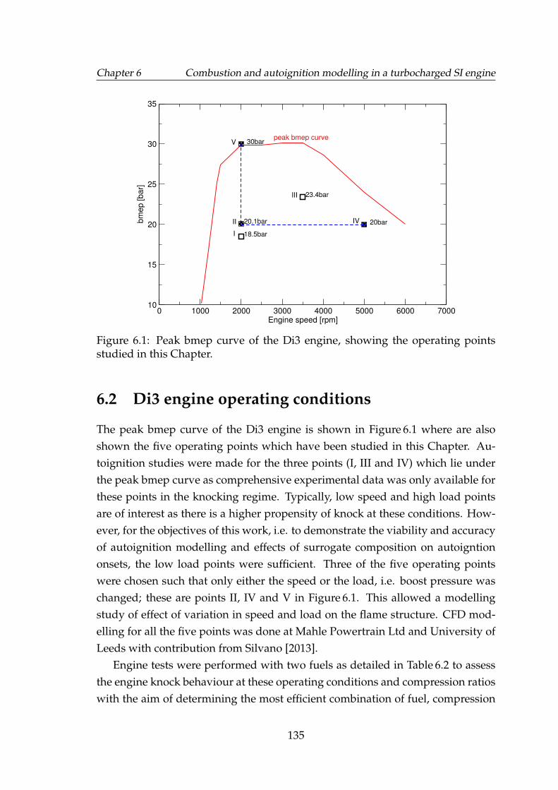
Chapter 6 Combustion and autoignition modelling in a turbocharged SI engine
20.1bar
30bar
20bar
18.5bar
23.4bar
0 1000 2000 3000 4000 5000 6000 7000Engine speed [rpm]
10
15
20
25
30
35
bm
ep [bar]
peak bmep curve
I
II
III
IV
V
Figure 6.1: Peak bmep curve of the Di3 engine, showing the operating pointsstudied in this Chapter.
6.2 Di3 engine operating conditions
The peak bmep curve of the Di3 engine is shown in Figure 6.1 where are alsoshown the five operating points which have been studied in this Chapter. Au-toignition studies were made for the three points (I, III and IV) which lie underthe peak bmep curve as comprehensive experimental data was only available forthese points in the knocking regime. Typically, low speed and high load pointsare of interest as there is a higher propensity of knock at these conditions. How-ever, for the objectives of this work, i.e. to demonstrate the viability and accuracyof autoignition modelling and effects of surrogate composition on autoigntiononsets, the low load points were sufficient. Three of the five operating pointswere chosen such that only either the speed or the load, i.e. boost pressure waschanged; these are points II, IV and V in Figure 6.1. This allowed a modellingstudy of effect of variation in speed and load on the flame structure. CFD mod-elling for all the five points was done at Mahle Powertrain Ltd and University ofLeeds with contribution from Silvano [2013].
Engine tests were performed with two fuels as detailed in Table 6.2 to assessthe engine knock behaviour at these operating conditions and compression ratioswith the aim of determining the most efficient combination of fuel, compression
135
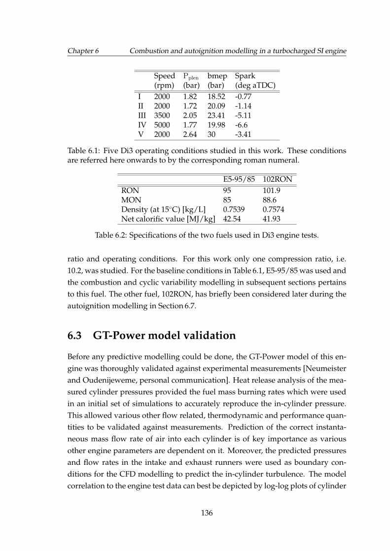
Chapter 6 Combustion and autoignition modelling in a turbocharged SI engine
Speed Pplen bmep Spark(rpm) (bar) (bar) (deg aTDC)
I 2000 1.82 18.52 -0.77II 2000 1.72 20.09 -1.14III 3500 2.05 23.41 -5.11IV 5000 1.77 19.98 -6.6V 2000 2.64 30 -3.41
Table 6.1: Five Di3 operating conditions studied in this work. These conditionsare referred here onwards to by the corresponding roman numeral.
E5-95/85 102RONRON 95 101.9MON 85 88.6Density (at 15◦C) [kg/L] 0.7539 0.7574Net calorific value [MJ/kg] 42.54 41.93
Table 6.2: Specifications of the two fuels used in Di3 engine tests.
ratio and operating conditions. For this work only one compression ratio, i.e.10.2, was studied. For the baseline conditions in Table 6.1, E5-95/85 was used andthe combustion and cyclic variability modelling in subsequent sections pertainsto this fuel. The other fuel, 102RON, has briefly been considered later during theautoignition modelling in Section 6.7.
6.3 GT-Power model validation
Before any predictive modelling could be done, the GT-Power model of this en-gine was thoroughly validated against experimental measurements [Neumeisterand Oudenijeweme, personal communication]. Heat release analysis of the mea-sured cylinder pressures provided the fuel mass burning rates which were usedin an initial set of simulations to accurately reproduce the in-cylinder pressure.This allowed various other flow related, thermodynamic and performance quan-tities to be validated against measurements. Prediction of the correct instanta-neous mass flow rate of air into each cylinder is of key importance as variousother engine parameters are dependent on it. Moreover, the predicted pressuresand flow rates in the intake and exhaust runners were used as boundary con-ditions for the CFD modelling to predict the in-cylinder turbulence. The modelcorrelation to the engine test data can best be depicted by log-log plots of cylinder
136
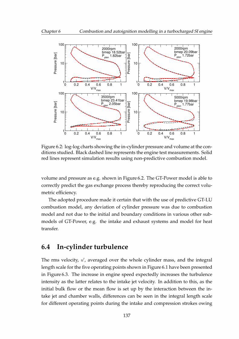
Chapter 6 Combustion and autoignition modelling in a turbocharged SI engine
0 0.2 0.4 0.6 0.8 1V/V
max
1
10
100
Pre
ssure
[bar]
0 0.2 0.4 0.6 0.8 1V/V
max
1
10
100
Pre
ssure
[bar]
0 0.2 0.4 0.6 0.8 1V/V
max
1
10
100
Pre
ssure
[bar]
0 0.2 0.4 0.6 0.8 1V/V
max
1
10
100
Pre
ssure
[bar]
2000rpmbmep 18.52barP
plen 1.82bar
2000rpmbmep 20.09barP
plen 1.72bar
5000rpmbmep 19.98barP
plen 1.77bar
3500rpmbmep 23.41barP
plen 2.05bar
Figure 6.2: log-log charts showing the in-cylinder pressure and volume at the con-ditions studied. Black dashed line represents the engine test measurements. Solidred lines represent simulation results using non-predictive combustion model.
volume and pressure as e.g. shown in Figure 6.2. The GT-Power model is able tocorrectly predict the gas exchange process thereby reproducing the correct volu-metric efficiency.
The adopted procedure made it certain that with the use of predictive GT-LUcombustion model, any deviation of cylinder pressure was due to combustionmodel and not due to the initial and boundary conditions in various other sub-models of GT-Power, e.g. the intake and exhaust systems and model for heattransfer.
6.4 In-cylinder turbulence
The rms velocity, u′, averaged over the whole cylinder mass, and the integrallength scale for the five operating points shown in Figure 6.1 have been presentedin Figure 6.3. The increase in engine speed expectedly increases the turbulenceintensity as the latter relates to the intake jet velocity. In addition to this, as theinitial bulk flow or the mean flow is set up by the interaction between the in-take jet and chamber walls, differences can be seen in the integral length scalefor different operating points during the intake and compression strokes owing
137
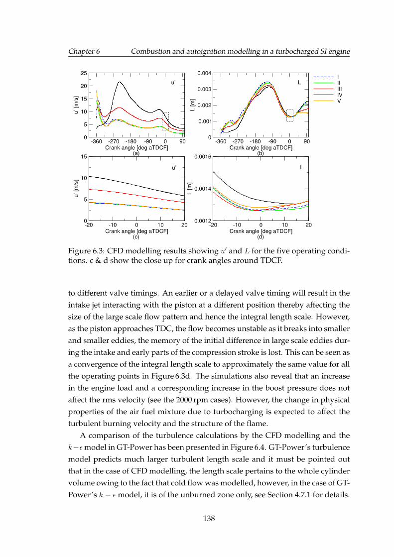
Chapter 6 Combustion and autoignition modelling in a turbocharged SI engine
-360 -270 -180 -90 0 90Crank angle [deg aTDCF] (a)
0
5
10
15
20
25u
’ [m
/s]
I II IIIIV V
-360 -270 -180 -90 0 90Crank angle [deg aTDCF] (b)
0
0.001
0.002
0.003
0.004
L [
m]
-20 -10 0 10 20Crank angle [deg aTDCF] (c)
0
5
10
15
u’ [m
/s]
-20 -10 0 10 20Crank angle [deg aTDCF] (d)
0.0012
0.0014
0.0016
L [
m]
u’
u’ L
L
Figure 6.3: CFD modelling results showing u′ and L for the five operating condi-tions. c & d show the close up for crank angles around TDCF.
to different valve timings. An earlier or a delayed valve timing will result in theintake jet interacting with the piston at a different position thereby affecting thesize of the large scale flow pattern and hence the integral length scale. However,as the piston approaches TDC, the flow becomes unstable as it breaks into smallerand smaller eddies, the memory of the initial difference in large scale eddies dur-ing the intake and early parts of the compression stroke is lost. This can be seen asa convergence of the integral length scale to approximately the same value for allthe operating points in Figure 6.3d. The simulations also reveal that an increasein the engine load and a corresponding increase in the boost pressure does notaffect the rms velocity (see the 2000 rpm cases). However, the change in physicalproperties of the air fuel mixture due to turbocharging is expected to affect theturbulent burning velocity and the structure of the flame.
A comparison of the turbulence calculations by the CFD modelling and thek−εmodel in GT-Power has been presented in Figure 6.4. GT-Power’s turbulencemodel predicts much larger turbulent length scale and it must be pointed outthat in the case of CFD modelling, the length scale pertains to the whole cylindervolume owing to the fact that cold flow was modelled, however, in the case of GT-Power’s k − ε model, it is of the unburned zone only, see Section 4.7.1 for details.
138
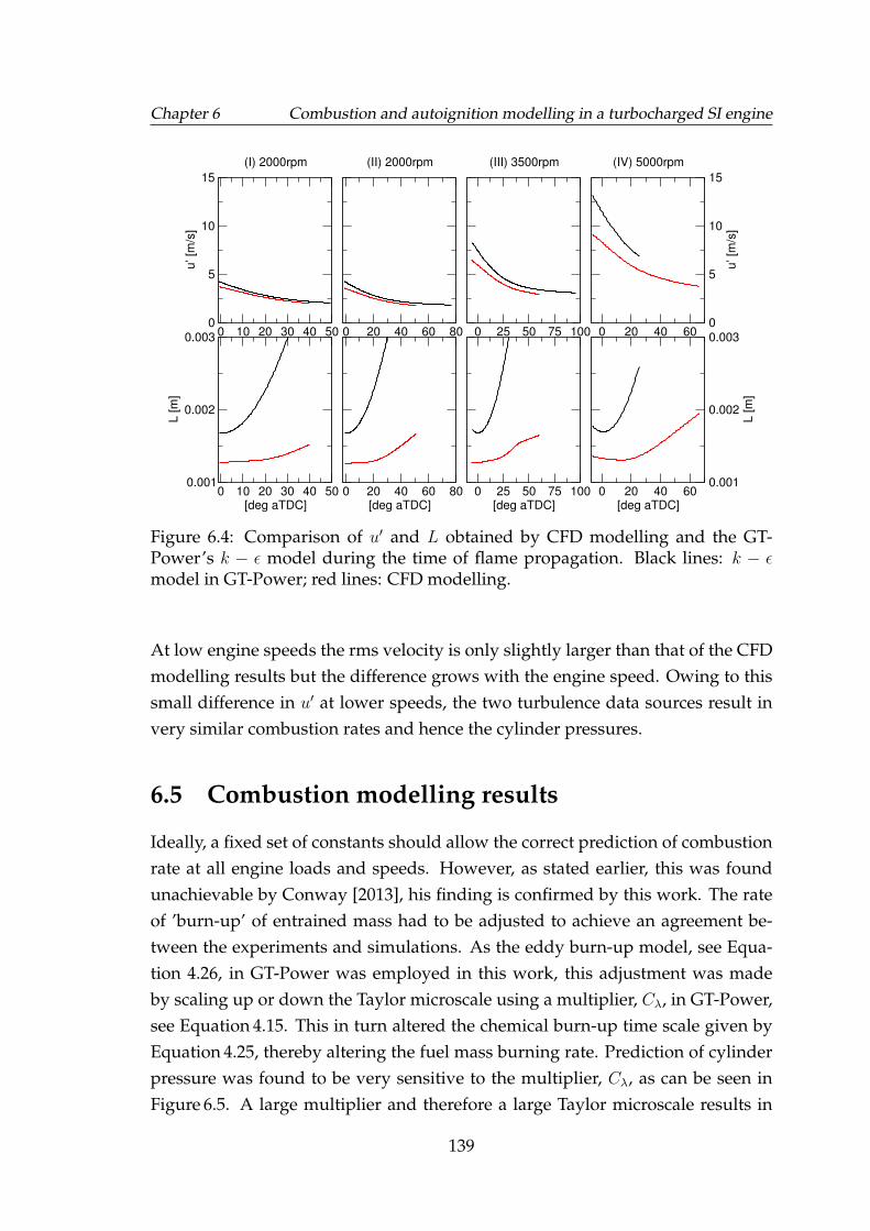
Chapter 6 Combustion and autoignition modelling in a turbocharged SI engine
0 10 20 30 40 500
5
10
15u
’ [m
/s]
(I) 2000rpm
0 10 20 30 40 50[deg aTDC]
0.001
0.002
0.003
L [
m]
0 20 40 60 80
(II) 2000rpm
0 20 40 60 80[deg aTDC]
0 25 50 75 100
(III) 3500rpm
0 25 50 75 100[deg aTDC]
0 20 40 600
5
10
15
u’ [m
/s]
(IV) 5000rpm
0 20 40 60[deg aTDC]
0.001
0.002
0.003
L [
m]
Figure 6.4: Comparison of u′ and L obtained by CFD modelling and the GT-Power’s k − ε model during the time of flame propagation. Black lines: k − εmodel in GT-Power; red lines: CFD modelling.
At low engine speeds the rms velocity is only slightly larger than that of the CFDmodelling results but the difference grows with the engine speed. Owing to thissmall difference in u′ at lower speeds, the two turbulence data sources result invery similar combustion rates and hence the cylinder pressures.
6.5 Combustion modelling results
Ideally, a fixed set of constants should allow the correct prediction of combustionrate at all engine loads and speeds. However, as stated earlier, this was foundunachievable by Conway [2013], his finding is confirmed by this work. The rateof ’burn-up’ of entrained mass had to be adjusted to achieve an agreement be-tween the experiments and simulations. As the eddy burn-up model, see Equa-tion 4.26, in GT-Power was employed in this work, this adjustment was madeby scaling up or down the Taylor microscale using a multiplier, Cλ, in GT-Power,see Equation 4.15. This in turn altered the chemical burn-up time scale given byEquation 4.25, thereby altering the fuel mass burning rate. Prediction of cylinderpressure was found to be very sensitive to the multiplier, Cλ, as can be seen inFigure 6.5. A large multiplier and therefore a large Taylor microscale results in
139
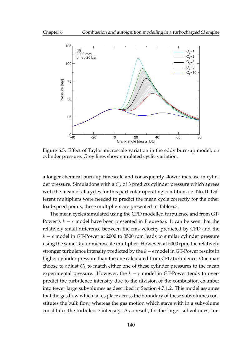
Chapter 6 Combustion and autoignition modelling in a turbocharged SI engine
-40 -20 0 20 40 60 80Crank angle [deg aTDC]
0
25
50
75
100
125
Pre
ssure
[bar]
Cλ=1
Cλ=2
Cλ=3
Cλ=5
Cλ=10
(II)2000 rpmbmep 20 bar
Figure 6.5: Effect of Taylor microscale variation in the eddy burn-up model, oncylinder pressure. Grey lines show simulated cyclic variation.
a longer chemical burn-up timescale and consequently slower increase in cylin-der pressure. Simulations with a Cλ of 3 predicts cylinder pressure which agreeswith the mean of all cycles for this particular operating condition, i.e. No. II. Dif-ferent multipliers were needed to predict the mean cycle correctly for the otherload-speed points, these multipliers are presented in Table 6.3.
The mean cycles simulated using the CFD modelled turbulence and from GT-Power’s k − ε model have been presented in Figure 6.6. It can be seen that therelatively small difference between the rms velocity predicted by CFD and thek − ε model in GT-Power at 2000 to 3500 rpm leads to similar cylinder pressureusing the same Taylor microscale multiplier. However, at 5000 rpm, the relativelystronger turbulence intensity predicted by the k− ε model in GT-Power results inhigher cylinder pressure than the one calculated from CFD turbulence. One maychoose to adjust Cλ to match either one of these cylinder pressures to the meanexperimental pressure. However, the k − ε model in GT-Power tends to over-predict the turbulence intensity due to the division of the combustion chamberinto fewer large subvolumes as described in Section 4.7.1.2. This model assumesthat the gas flow which takes place across the boundary of these subvolumes con-stitutes the bulk flow, whereas the gas motion which stays with in a subvolumeconstitutes the turbulence intensity. As a result, for the larger subvolumes, tur-
140
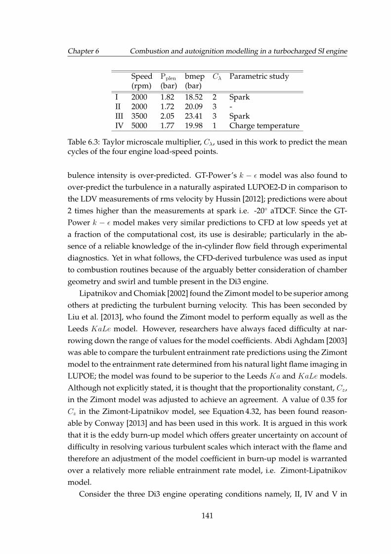
Chapter 6 Combustion and autoignition modelling in a turbocharged SI engine
Speed Pplen bmep Cλ Parametric study(rpm) (bar) (bar)
I 2000 1.82 18.52 2 SparkII 2000 1.72 20.09 3 -III 3500 2.05 23.41 3 SparkIV 5000 1.77 19.98 1 Charge temperature
Table 6.3: Taylor microscale multiplier, Cλ, used in this work to predict the meancycles of the four engine load-speed points.
bulence intensity is over-predicted. GT-Power’s k − ε model was also found toover-predict the turbulence in a naturally aspirated LUPOE2-D in comparison tothe LDV measurements of rms velocity by Hussin [2012]; predictions were about2 times higher than the measurements at spark i.e. -20◦ aTDCF. Since the GT-Power k − ε model makes very similar predictions to CFD at low speeds yet ata fraction of the computational cost, its use is desirable; particularly in the ab-sence of a reliable knowledge of the in-cylinder flow field through experimentaldiagnostics. Yet in what follows, the CFD-derived turbulence was used as inputto combustion routines because of the arguably better consideration of chambergeometry and swirl and tumble present in the Di3 engine.
Lipatnikov and Chomiak [2002] found the Zimont model to be superior amongothers at predicting the turbulent burning velocity. This has been seconded byLiu et al. [2013], who found the Zimont model to perform equally as well as theLeeds KaLe model. However, researchers have always faced difficulty at nar-rowing down the range of values for the model coefficients. Abdi Aghdam [2003]was able to compare the turbulent entrainment rate predictions using the Zimontmodel to the entrainment rate determined from his natural light flame imaging inLUPOE; the model was found to be superior to the Leeds Ka and KaLe models.Although not explicitly stated, it is thought that the proportionality constant, Cz,in the Zimont model was adjusted to achieve an agreement. A value of 0.35 forCz in the Zimont-Lipatnikov model, see Equation 4.32, has been found reason-able by Conway [2013] and has been used in this work. It is argued in this workthat it is the eddy burn-up model which offers greater uncertainty on account ofdifficulty in resolving various turbulent scales which interact with the flame andtherefore an adjustment of the model coefficient in burn-up model is warrantedover a relatively more reliable entrainment rate model, i.e. Zimont-Lipatnikovmodel.
Consider the three Di3 engine operating conditions namely, II, IV and V in
141
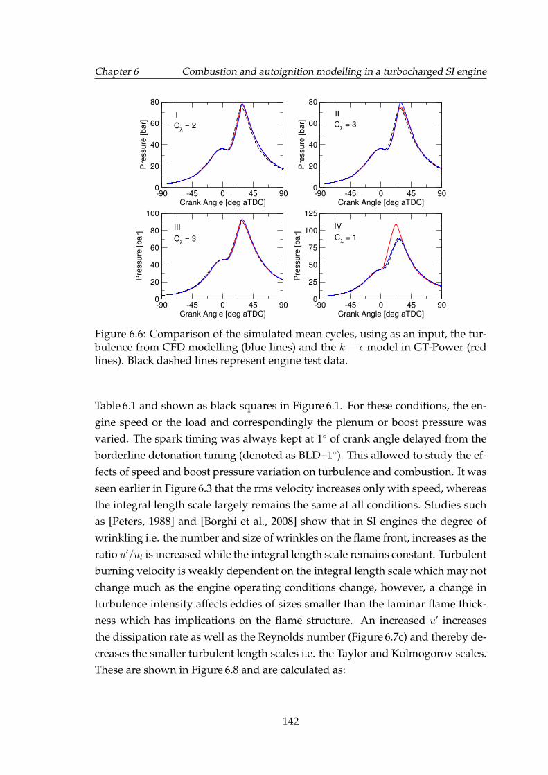
Chapter 6 Combustion and autoignition modelling in a turbocharged SI engine
-90 -45 0 45 90Crank Angle [deg aTDC]
0
20
40
60
80
Pre
ssure
[bar]
-90 -45 0 45 90Crank Angle [deg aTDC]
0
20
40
60
80
Pre
ssure
[bar]
-90 -45 0 45 90Crank Angle [deg aTDC]
0
20
40
60
80
100
Pre
ssure
[bar]
-90 -45 0 45 90Crank Angle [deg aTDC]
0
25
50
75
100
125
Pre
ssure
[bar]
I II
III IV
Cλ = 2 C
λ = 3
Cλ = 3 C
λ = 1
Figure 6.6: Comparison of the simulated mean cycles, using as an input, the tur-bulence from CFD modelling (blue lines) and the k − ε model in GT-Power (redlines). Black dashed lines represent engine test data.
Table 6.1 and shown as black squares in Figure 6.1. For these conditions, the en-gine speed or the load and correspondingly the plenum or boost pressure wasvaried. The spark timing was always kept at 1◦ of crank angle delayed from theborderline detonation timing (denoted as BLD+1◦). This allowed to study the ef-fects of speed and boost pressure variation on turbulence and combustion. It wasseen earlier in Figure 6.3 that the rms velocity increases only with speed, whereasthe integral length scale largely remains the same at all conditions. Studies suchas [Peters, 1988] and [Borghi et al., 2008] show that in SI engines the degree ofwrinkling i.e. the number and size of wrinkles on the flame front, increases as theratio u′/ul is increased while the integral length scale remains constant. Turbulentburning velocity is weakly dependent on the integral length scale which may notchange much as the engine operating conditions change, however, a change inturbulence intensity affects eddies of sizes smaller than the laminar flame thick-ness which has implications on the flame structure. An increased u′ increasesthe dissipation rate as well as the Reynolds number (Figure 6.7c) and thereby de-creases the smaller turbulent length scales i.e. the Taylor and Kolmogorov scales.These are shown in Figure 6.8 and are calculated as:
142
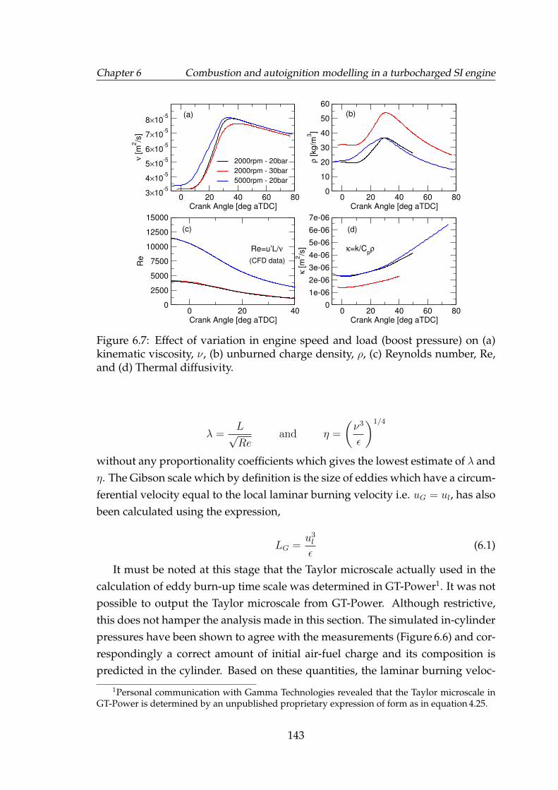
Chapter 6 Combustion and autoignition modelling in a turbocharged SI engine
0 20 40 60 80Crank Angle [deg aTDC]
3×10⁻⁵
4×10⁻⁵
5×10⁻⁵
6×10⁻⁵
7×10⁻⁵
8×10⁻⁵
ν [m
2/s
]
2000rpm - 20bar
2000rpm - 30bar
5000rpm - 20bar
0 20 40 60 80Crank Angle [deg aTDC]
0
10
20
30
40
50
60
ρ [kg/m
3]
0 20 40Crank Angle [deg aTDC]
0
2500
5000
7500
10000
12500
15000
Re
0 20 40 60 80Crank Angle [deg aTDC]
0
1e-06
2e-06
3e-06
4e-06
5e-06
6e-06
7e-06
κ [m
2/s
] κ=k/CpρRe=u’L/ν
(a) (b)
(c) (d)
(CFD data)
Figure 6.7: Effect of variation in engine speed and load (boost pressure) on (a)kinematic viscosity, ν, (b) unburned charge density, ρ, (c) Reynolds number, Re,and (d) Thermal diffusivity.
λ =L√Re
and η =
(ν3
ε
)1/4
without any proportionality coefficients which gives the lowest estimate of λ andη. The Gibson scale which by definition is the size of eddies which have a circum-ferential velocity equal to the local laminar burning velocity i.e. uG = ul, has alsobeen calculated using the expression,
LG =u3l
ε(6.1)
It must be noted at this stage that the Taylor microscale actually used in thecalculation of eddy burn-up time scale was determined in GT-Power1. It was notpossible to output the Taylor microscale from GT-Power. Although restrictive,this does not hamper the analysis made in this section. The simulated in-cylinderpressures have been shown to agree with the measurements (Figure 6.6) and cor-respondingly a correct amount of initial air-fuel charge and its composition ispredicted in the cylinder. Based on these quantities, the laminar burning veloc-
1Personal communication with Gamma Technologies revealed that the Taylor microscale inGT-Power is determined by an unpublished proprietary expression of form as in equation 4.25.
143
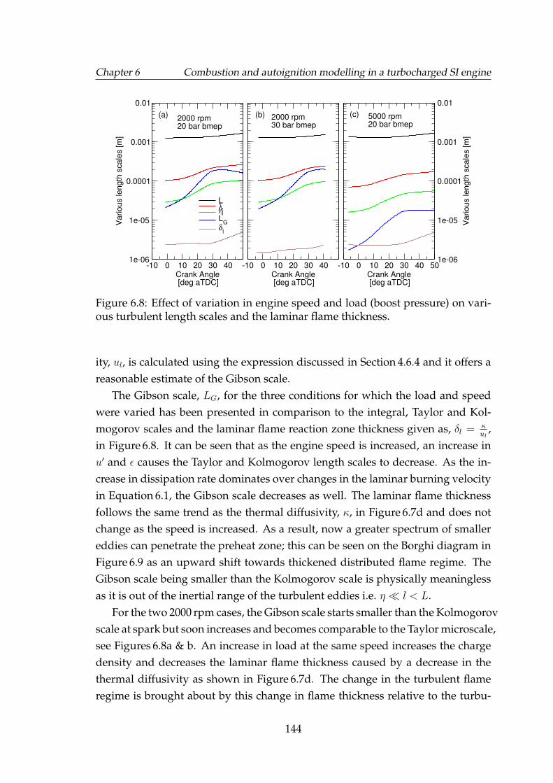
Chapter 6 Combustion and autoignition modelling in a turbocharged SI engine
-10 0 10 20 30 40Crank Angle [deg aTDC]
1e-06
1e-05
0.0001
0.001
0.01
Various length
scale
s [m
]
LληL
Gδ
l
-10 0 10 20 30 40Crank Angle [deg aTDC]
-10 0 10 20 30 40 50Crank Angle [deg aTDC]
1e-06
1e-05
0.0001
0.001
0.01
Various length
scale
s [m
]
2000 rpm20 bar bmep
2000 rpm30 bar bmep
5000 rpm20 bar bmep
(a) (b) (c)
Figure 6.8: Effect of variation in engine speed and load (boost pressure) on vari-ous turbulent length scales and the laminar flame thickness.
ity, ul, is calculated using the expression discussed in Section 4.6.4 and it offers areasonable estimate of the Gibson scale.
The Gibson scale, LG, for the three conditions for which the load and speedwere varied has been presented in comparison to the integral, Taylor and Kol-mogorov scales and the laminar flame reaction zone thickness given as, δl = κ
ul,
in Figure 6.8. It can be seen that as the engine speed is increased, an increase inu′ and ε causes the Taylor and Kolmogorov length scales to decrease. As the in-crease in dissipation rate dominates over changes in the laminar burning velocityin Equation 6.1, the Gibson scale decreases as well. The laminar flame thicknessfollows the same trend as the thermal diffusivity, κ, in Figure 6.7d and does notchange as the speed is increased. As a result, now a greater spectrum of smallereddies can penetrate the preheat zone; this can be seen on the Borghi diagram inFigure 6.9 as an upward shift towards thickened distributed flame regime. TheGibson scale being smaller than the Kolmogorov scale is physically meaninglessas it is out of the inertial range of the turbulent eddies i.e. η � l < L.
For the two 2000 rpm cases, the Gibson scale starts smaller than the Kolmogorovscale at spark but soon increases and becomes comparable to the Taylor microscale,see Figures 6.8a & b. An increase in load at the same speed increases the chargedensity and decreases the laminar flame thickness caused by a decrease in thethermal diffusivity as shown in Figure 6.7d. The change in the turbulent flameregime is brought about by this change in flame thickness relative to the turbu-
144
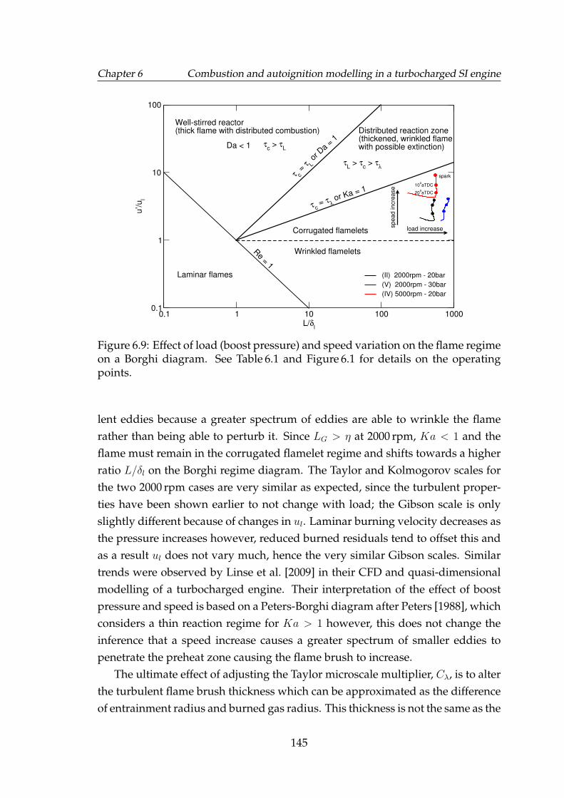
Chapter 6 Combustion and autoignition modelling in a turbocharged SI engine
0.1 1 10 100 1000L/δ
l
0.1
1
10
100
u’/u
l
(II) 2000rpm - 20bar
(V) 2000rpm - 30bar
(IV) 5000rpm - 20bar
Laminar flames
Well-stirred reactor(thick flame with distributed combustion) Distributed reaction zone
(thickened, wrinkled flamewith possible extinction)
Corrugated flamelets
Wrinkled flameletsRe = 1
τ c = τ λ
or Ka = 1
load increase
τL > τ
c > τ
λ
τc > τ
L
τ c =
τ L o
r Da
= 1Da < 1
spead incre
ase
spark
10oaTDC
20oaTDC
Figure 6.9: Effect of load (boost pressure) and speed variation on the flame regimeon a Borghi diagram. See Table 6.1 and Figure 6.1 for details on the operatingpoints.
lent eddies because a greater spectrum of eddies are able to wrinkle the flamerather than being able to perturb it. Since LG > η at 2000 rpm, Ka < 1 and theflame must remain in the corrugated flamelet regime and shifts towards a higherratio L/δl on the Borghi regime diagram. The Taylor and Kolmogorov scales forthe two 2000 rpm cases are very similar as expected, since the turbulent proper-ties have been shown earlier to not change with load; the Gibson scale is onlyslightly different because of changes in ul. Laminar burning velocity decreases asthe pressure increases however, reduced burned residuals tend to offset this andas a result ul does not vary much, hence the very similar Gibson scales. Similartrends were observed by Linse et al. [2009] in their CFD and quasi-dimensionalmodelling of a turbocharged engine. Their interpretation of the effect of boostpressure and speed is based on a Peters-Borghi diagram after Peters [1988], whichconsiders a thin reaction regime for Ka > 1 however, this does not change theinference that a speed increase causes a greater spectrum of smaller eddies topenetrate the preheat zone causing the flame brush to increase.
The ultimate effect of adjusting the Taylor microscale multiplier, Cλ, is to alterthe turbulent flame brush thickness which can be approximated as the differenceof entrainment radius and burned gas radius. This thickness is not the same as the
145
Chapter 6 Combustion and autoignition modelling in a turbocharged SI engine
one given by Equation 4.35 which is dependent only on the large scale turbulenceand mathematically independent of any modification of the Taylor microscale. Alarger multiplier results in a thicker flame brush. The simulations show that asthe engine speed is decreased and/or the load is increased, there is a requirementfor the Taylor multiplier to be increased i.e. the flame brush should be thicker.This seems contradictory to the flame regime analysis in preceding paragraphs.The requirement for Taylor microscale adjustment in the burn-up model in anapparently contradictory manner to the expected changes in flame structure canbe caused by a number of reasons. The experimentally determined quantities arethought to be reliable and an unlikely source of model disagreement as widelyused tried and tested techniques are employed in measuring such quantities. Theother possible sources can be, the CFD data, u′ and L, the smaller scales of tur-bulence which are determined using expressions presented in Section 4.2.1.2 anda similar proprietary expression in GT-Power, an inaccurate estimate of the lam-inar burning velocity, or the entrainment model itself. The CFD data, althoughpossibly inaccurate, cannot cause this as in such a case a single Taylor microscalemultiplier will be expected to work for all the engine conditions i.e. if the CFDpredictions are wrong by the same magnitude for all the conditions.
The expression for ul, Equation 4.37, as presented in Section 4.6.4 has beenshown by Sileghem et al. [2013] to use a higher value of the power exponent fortemperature dependence than observed in their experiments for a commercialgasoline. Also, it is likely that the combustion instability behaviour of the E5-95/85 gasoline in this work is different from the gasoline for which the expressionfor laminar burning velocity, Equation 4.37, was derived. Moreover, the effects offlame stretch and thermo-diffusive instability are carefully avoided during mea-surements of laminar flame speed, on basis of which the empirical expressions forul are then determined. So any flame instability which may actually be presentin the engine is neglected in the analysis presented above introducing uncertain-ties. Any inaccuracies in ul will have significant effect on the after-burning as thechemical eddy burn-up time is calculated as τb = λ/ul. Validation of the burningvelocity expressions at high p− T conditions of engines such as the Di3 engine isnot possible owing to insufficient ul measurements and particularly the onset ofinstabilities at those conditions.
The calculation of Taylor microscale in GT-Power and the entrainment modelmay also be significant sources of inaccuracies. The Zimont model treats the tur-bulent eddies of size smaller than the laminar flame thickness to affect the local
146
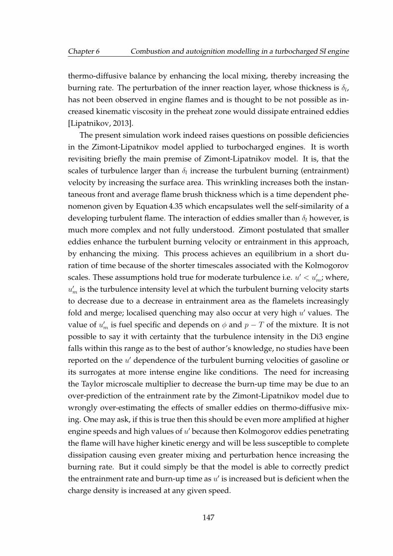
Chapter 6 Combustion and autoignition modelling in a turbocharged SI engine
thermo-diffusive balance by enhancing the local mixing, thereby increasing theburning rate. The perturbation of the inner reaction layer, whose thickness is δl,has not been observed in engine flames and is thought to be not possible as in-creased kinematic viscosity in the preheat zone would dissipate entrained eddies[Lipatnikov, 2013].
The present simulation work indeed raises questions on possible deficienciesin the Zimont-Lipatnikov model applied to turbocharged engines. It is worthrevisiting briefly the main premise of Zimont-Lipatnikov model. It is, that thescales of turbulence larger than δl increase the turbulent burning (entrainment)velocity by increasing the surface area. This wrinkling increases both the instan-taneous front and average flame brush thickness which is a time dependent phe-nomenon given by Equation 4.35 which encapsulates well the self-similarity of adeveloping turbulent flame. The interaction of eddies smaller than δl however, ismuch more complex and not fully understood. Zimont postulated that smallereddies enhance the turbulent burning velocity or entrainment in this approach,by enhancing the mixing. This process achieves an equilibrium in a short du-ration of time because of the shorter timescales associated with the Kolmogorovscales. These assumptions hold true for moderate turbulence i.e. u′ < u′m; where,u′m is the turbulence intensity level at which the turbulent burning velocity startsto decrease due to a decrease in entrainment area as the flamelets increasinglyfold and merge; localised quenching may also occur at very high u′ values. Thevalue of u′m is fuel specific and depends on φ and p − T of the mixture. It is notpossible to say it with certainty that the turbulence intensity in the Di3 enginefalls within this range as to the best of author’s knowledge, no studies have beenreported on the u′ dependence of the turbulent burning velocities of gasoline orits surrogates at more intense engine like conditions. The need for increasingthe Taylor microscale multiplier to decrease the burn-up time may be due to anover-prediction of the entrainment rate by the Zimont-Lipatnikov model due towrongly over-estimating the effects of smaller eddies on thermo-diffusive mix-ing. One may ask, if this is true then this should be even more amplified at higherengine speeds and high values of u′ because then Kolmogorov eddies penetratingthe flame will have higher kinetic energy and will be less susceptible to completedissipation causing even greater mixing and perturbation hence increasing theburning rate. But it could simply be that the model is able to correctly predictthe entrainment rate and burn-up time as u′ is increased but is deficient when thecharge density is increased at any given speed.
147
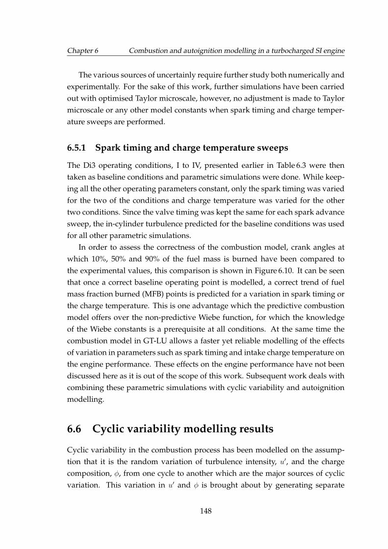
Chapter 6 Combustion and autoignition modelling in a turbocharged SI engine
The various sources of uncertainly require further study both numerically andexperimentally. For the sake of this work, further simulations have been carriedout with optimised Taylor microscale, however, no adjustment is made to Taylormicroscale or any other model constants when spark timing and charge temper-ature sweeps are performed.
6.5.1 Spark timing and charge temperature sweeps
The Di3 operating conditions, I to IV, presented earlier in Table 6.3 were thentaken as baseline conditions and parametric simulations were done. While keep-ing all the other operating parameters constant, only the spark timing was variedfor the two of the conditions and charge temperature was varied for the othertwo conditions. Since the valve timing was kept the same for each spark advancesweep, the in-cylinder turbulence predicted for the baseline conditions was usedfor all other parametric simulations.
In order to assess the correctness of the combustion model, crank angles atwhich 10%, 50% and 90% of the fuel mass is burned have been compared tothe experimental values, this comparison is shown in Figure 6.10. It can be seenthat once a correct baseline operating point is modelled, a correct trend of fuelmass fraction burned (MFB) points is predicted for a variation in spark timing orthe charge temperature. This is one advantage which the predictive combustionmodel offers over the non-predictive Wiebe function, for which the knowledgeof the Wiebe constants is a prerequisite at all conditions. At the same time thecombustion model in GT-LU allows a faster yet reliable modelling of the effectsof variation in parameters such as spark timing and intake charge temperature onthe engine performance. These effects on the engine performance have not beendiscussed here as it is out of the scope of this work. Subsequent work deals withcombining these parametric simulations with cyclic variability and autoignitionmodelling.
6.6 Cyclic variability modelling results
Cyclic variability in the combustion process has been modelled on the assump-tion that it is the random variation of turbulence intensity, u′, and the chargecomposition, φ, from one cycle to another which are the major sources of cyclicvariation. This variation in u′ and φ is brought about by generating separate
148
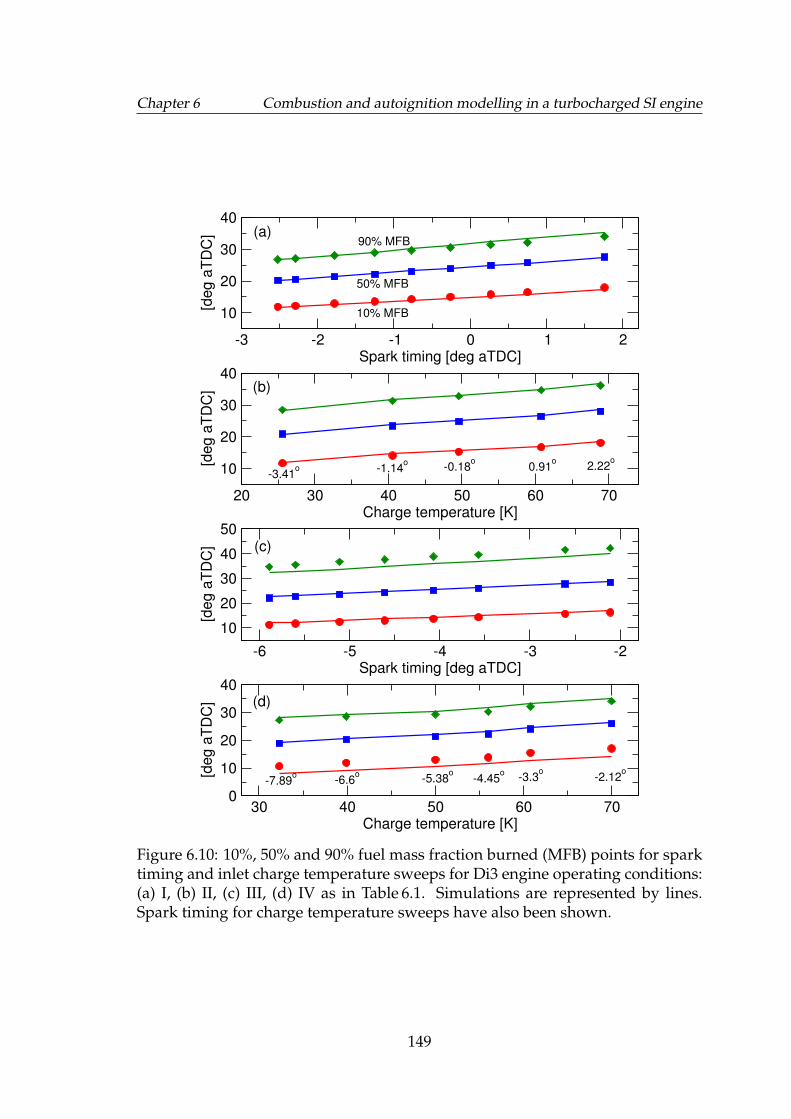
Chapter 6 Combustion and autoignition modelling in a turbocharged SI engine
-3 -2 -1 0 1 2Spark timing [deg aTDC]
10
20
30
40[d
eg a
TD
C]
20 30 40 50 60 70Charge temperature [K]
10
20
30
40
[deg a
TD
C]
-6 -5 -4 -3 -2Spark timing [deg aTDC]
10
20
30
40
50
[deg a
TD
C]
30 40 50 60 70Charge temperature [K]
0
10
20
30
40
[deg a
TD
C]
2.22o
0.91o
-0.18o
-1.14o
-3.41o
-2.12o
-3.3o
-4.45o
-5.38o
-6.6o
-7.89o
10% MFB
50% MFB
90% MFB(a)
(b)
(c)
(d)
Figure 6.10: 10%, 50% and 90% fuel mass fraction burned (MFB) points for sparktiming and inlet charge temperature sweeps for Di3 engine operating conditions:(a) I, (b) II, (c) III, (d) IV as in Table 6.1. Simulations are represented by lines.Spark timing for charge temperature sweeps have also been shown.
149
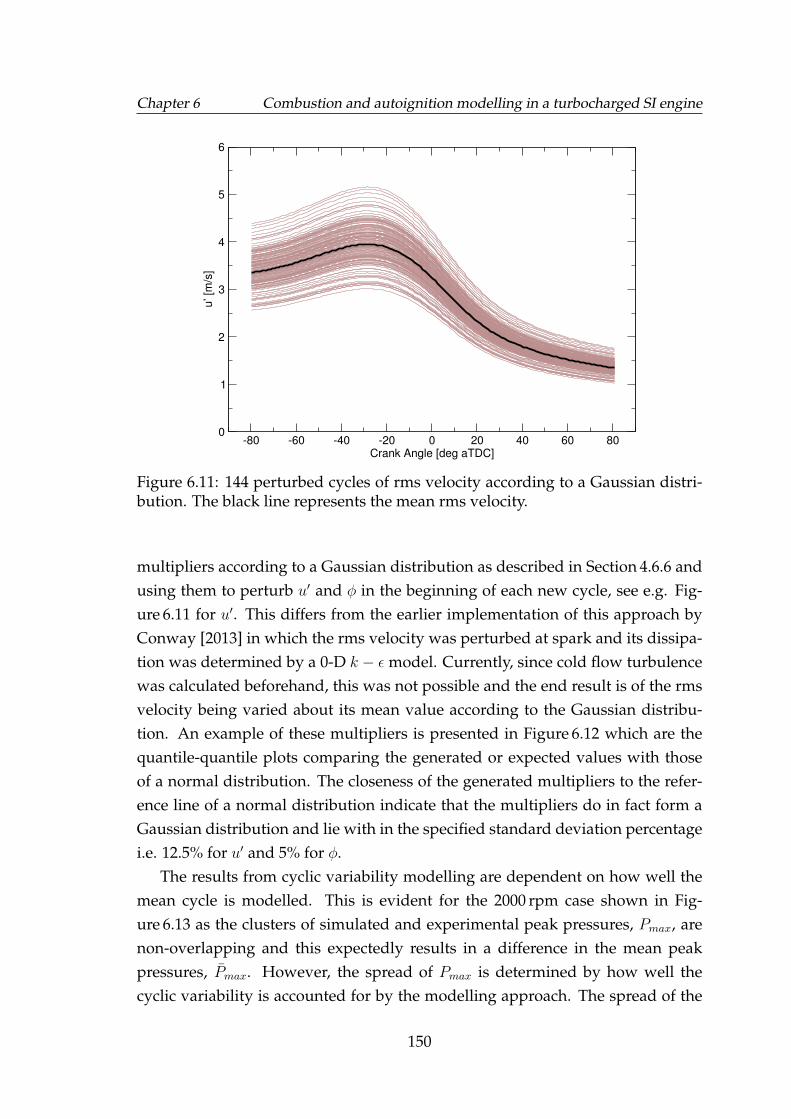
Chapter 6 Combustion and autoignition modelling in a turbocharged SI engine
-80 -60 -40 -20 0 20 40 60 80Crank Angle [deg aTDC]
0
1
2
3
4
5
6
u’ [m
/s]
Figure 6.11: 144 perturbed cycles of rms velocity according to a Gaussian distri-bution. The black line represents the mean rms velocity.
multipliers according to a Gaussian distribution as described in Section 4.6.6 andusing them to perturb u′ and φ in the beginning of each new cycle, see e.g. Fig-ure 6.11 for u′. This differs from the earlier implementation of this approach byConway [2013] in which the rms velocity was perturbed at spark and its dissipa-tion was determined by a 0-D k − ε model. Currently, since cold flow turbulencewas calculated beforehand, this was not possible and the end result is of the rmsvelocity being varied about its mean value according to the Gaussian distribu-tion. An example of these multipliers is presented in Figure 6.12 which are thequantile-quantile plots comparing the generated or expected values with thoseof a normal distribution. The closeness of the generated multipliers to the refer-ence line of a normal distribution indicate that the multipliers do in fact form aGaussian distribution and lie with in the specified standard deviation percentagei.e. 12.5% for u′ and 5% for φ.
The results from cyclic variability modelling are dependent on how well themean cycle is modelled. This is evident for the 2000 rpm case shown in Fig-ure 6.13 as the clusters of simulated and experimental peak pressures, Pmax, arenon-overlapping and this expectedly results in a difference in the mean peakpressures, Pmax. However, the spread of Pmax is determined by how well thecyclic variability is accounted for by the modelling approach. The spread of the
150
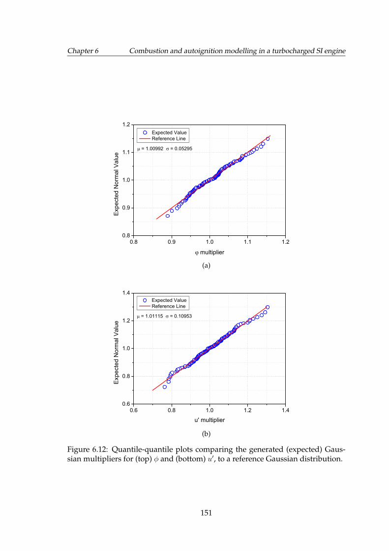
Chapter 6 Combustion and autoignition modelling in a turbocharged SI engine
0.8 0.9 1.0 1.1 1.20.8
0.9
1.0
1.1
1.2
= 1.00992 = 0.05295
Exp
ecte
d N
orm
al V
alue
multiplier
Expected Value Reference Line
(a)
0.6 0.8 1.0 1.2 1.40.6
0.8
1.0
1.2
1.4
= 1.01115 = 0.10953
Exp
ecte
d N
orm
al V
alue
u' multiplier
Expected Value Reference Line
(b)
Figure 6.12: Quantile-quantile plots comparing the generated (expected) Gaus-sian multipliers for (top) φ and (bottom) u′, to a reference Gaussian distribution.
151
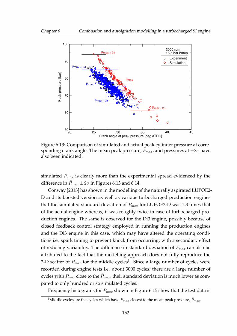
Chapter 6 Combustion and autoignition modelling in a turbocharged SI engine
20 25 30 35 40 45Crank angle at peak pressure [deg aTDC]
50
60
70
80
90
100
Peak p
ressure
[bar]
Experiment
Simulation
2000 rpm18.5 bar bmep
Pmax + 2σ
Pmax
Pmax - 2σ
Pmax
Pmax + 2σ
Pmax - 2σ
Figure 6.13: Comparison of simulated and actual peak cylinder pressure at corre-sponding crank angle. The mean peak pressure, Pmax, and pressures at ±2σ havealso been indicated.
simulated Pmax is clearly more than the experimental spread evidenced by thedifference in Pmax ± 2σ in Figures 6.13 and 6.14.
Conway [2013] has shown in the modelling of the naturally aspirated LUPOE2-D and its boosted version as well as various turbocharged production enginesthat the simulated standard deviation of Pmax for LUPOE2-D was 1.3 times thatof the actual engine whereas, it was roughly twice in case of turbocharged pro-duction engines. The same is observed for the Di3 engine, possibly because ofclosed feedback control strategy employed in running the production enginesand the Di3 engine in this case, which may have altered the operating condi-tions i.e. spark timing to prevent knock from occurring; with a secondary effectof reducing variability. The difference in standard deviation of Pmax can also beattributed to the fact that the modelling approach does not fully reproduce the2-D scatter of Pmax for the middle cycles1. Since a large number of cycles wererecorded during engine tests i.e. about 3000 cycles; there are a large number ofcycles with Pmax close to the Pmax, their standard deviation is much lower as com-pared to only hundred or so simulated cycles.
Frequency histograms for Pmax shown in Figure 6.15 show that the test data is
1Middle cycles are the cycles which have Pmax closest to the mean peak pressure, Pmax.
152
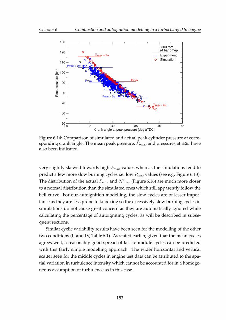
Chapter 6 Combustion and autoignition modelling in a turbocharged SI engine
20 25 30 35 40 45Crank angle at peak pressure [deg aTDC]
50
60
70
80
90
100
110
120
130
Peak p
ressure
[bar]
Experiment
Simulation
3500 rpm24 bar bmep
Pmax + 2σ
Pmax - 2σ
Pmax
Pmax + 2σ
Pmax
Pmax - 2σ
Figure 6.14: Comparison of simulated and actual peak cylinder pressure at corre-sponding crank angle. The mean peak pressure, Pmax, and pressures at ±2σ havealso been indicated.
very slightly skewed towards high Pmax values whereas the simulations tend topredict a few more slow burning cycles i.e. low Pmax values (see e.g. Figure 6.13).The distribution of the actual Pmax and θPmax (Figure 6.16) are much more closerto a normal distribution than the simulated ones which still apparently follow thebell curve. For our autoignition modelling, the slow cycles are of lesser impor-tance as they are less prone to knocking so the excessively slow burning cycles insimulations do not cause great concern as they are automatically ignored whilecalculating the percentage of autoigniting cycles, as will be described in subse-quent sections.
Similar cyclic variability results have been seen for the modelling of the othertwo conditions (II and IV, Table 6.1). As stated earlier, given that the mean cyclesagrees well, a reasonably good spread of fast to middle cycles can be predictedwith this fairly simple modelling approach. The wider horizontal and verticalscatter seen for the middle cycles in engine test data can be attributed to the spa-tial variation in turbulence intensity which cannot be accounted for in a homoge-neous assumption of turbulence as in this case.
153
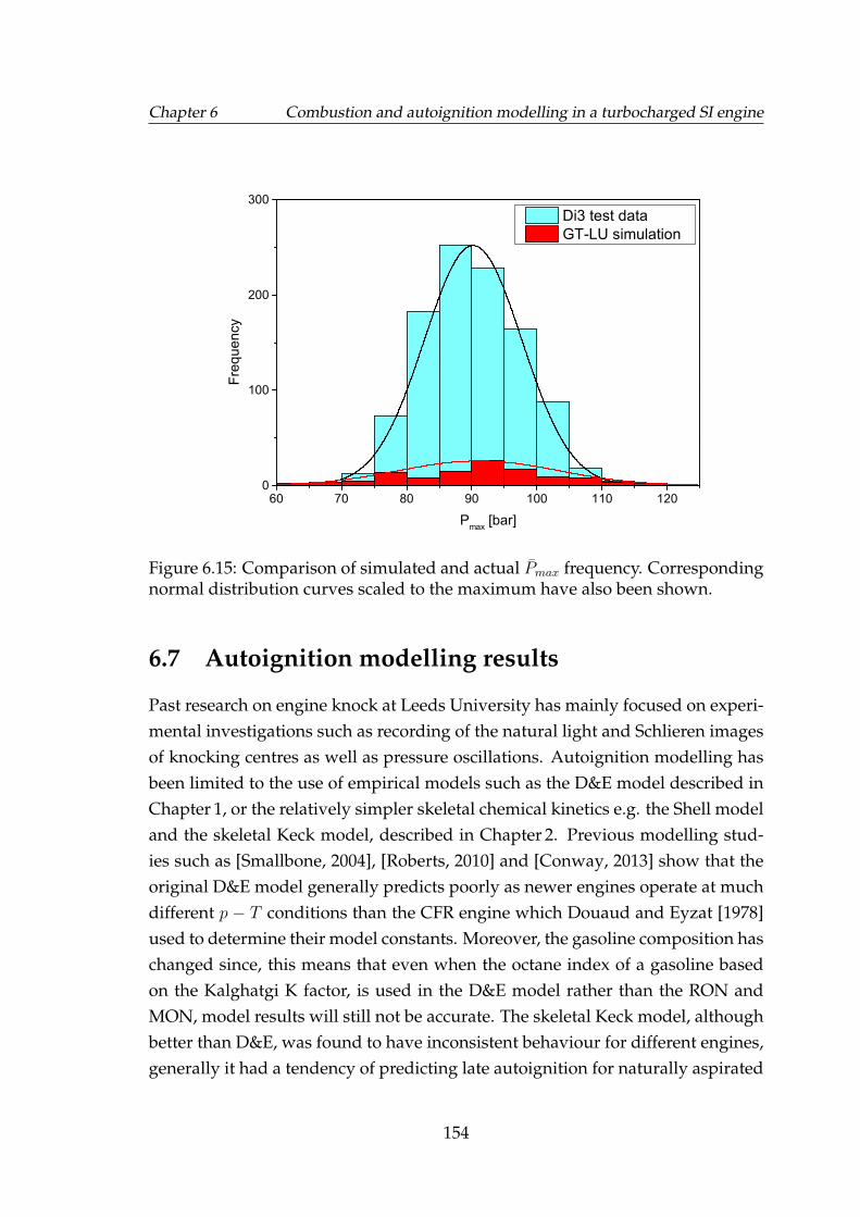
Chapter 6 Combustion and autoignition modelling in a turbocharged SI engine
60 70 80 90 100 110 1200
100
200
300
Freq
uenc
y
Pmax [bar]
Di3 test data GT-LU simulation
Figure 6.15: Comparison of simulated and actual Pmax frequency. Correspondingnormal distribution curves scaled to the maximum have also been shown.
6.7 Autoignition modelling results
Past research on engine knock at Leeds University has mainly focused on experi-mental investigations such as recording of the natural light and Schlieren imagesof knocking centres as well as pressure oscillations. Autoignition modelling hasbeen limited to the use of empirical models such as the D&E model described inChapter 1, or the relatively simpler skeletal chemical kinetics e.g. the Shell modeland the skeletal Keck model, described in Chapter 2. Previous modelling stud-ies such as [Smallbone, 2004], [Roberts, 2010] and [Conway, 2013] show that theoriginal D&E model generally predicts poorly as newer engines operate at muchdifferent p − T conditions than the CFR engine which Douaud and Eyzat [1978]used to determine their model constants. Moreover, the gasoline composition haschanged since, this means that even when the octane index of a gasoline basedon the Kalghatgi K factor, is used in the D&E model rather than the RON andMON, model results will still not be accurate. The skeletal Keck model, althoughbetter than D&E, was found to have inconsistent behaviour for different engines,generally it had a tendency of predicting late autoignition for naturally aspirated
154
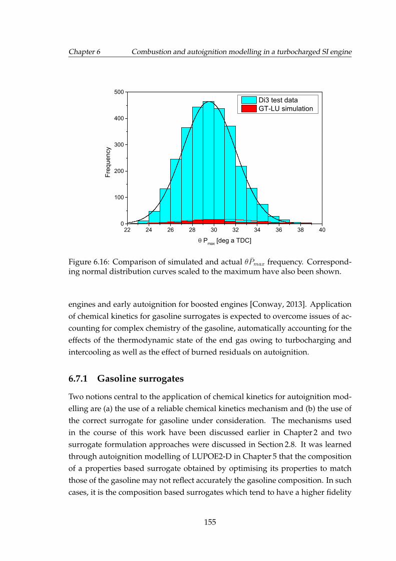
Chapter 6 Combustion and autoignition modelling in a turbocharged SI engine
22 24 26 28 30 32 34 36 38 400
100
200
300
400
500
Freq
uenc
y
Pmax [deg a TDC]
Di3 test data GT-LU simulation
Figure 6.16: Comparison of simulated and actual θPmax frequency. Correspond-ing normal distribution curves scaled to the maximum have also been shown.
engines and early autoignition for boosted engines [Conway, 2013]. Applicationof chemical kinetics for gasoline surrogates is expected to overcome issues of ac-counting for complex chemistry of the gasoline, automatically accounting for theeffects of the thermodynamic state of the end gas owing to turbocharging andintercooling as well as the effect of burned residuals on autoignition.
6.7.1 Gasoline surrogates
Two notions central to the application of chemical kinetics for autoignition mod-elling are (a) the use of a reliable chemical kinetics mechanism and (b) the use ofthe correct surrogate for gasoline under consideration. The mechanisms usedin the course of this work have been discussed earlier in Chapter 2 and twosurrogate formulation approaches were discussed in Section 2.8. It was learnedthrough autoignition modelling of LUPOE2-D in Chapter 5 that the compositionof a properties based surrogate obtained by optimising its properties to matchthose of the gasoline may not reflect accurately the gasoline composition. In suchcases, it is the composition based surrogates which tend to have a higher fidelity
155
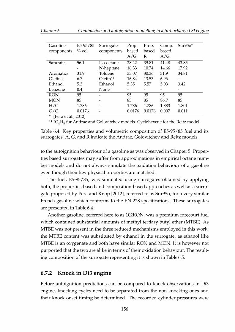
Chapter 6 Combustion and autoignition modelling in a turbocharged SI engine
Gasoline E5-95/85 Surrogate Prop. Prop. Comp. Sur95o*components % vol. components based based based
A/G R A/GSaturates 56.1 Iso-octane 28.42 39.81 41.48 43.85
- N-heptane 16.33 10.74 14.66 17.92Aromatics 31.9 Toluene 33.07 30.36 31.9 34.81Olefins 6.7 Olefin** 16.84 13.53 6.96 -Ethanol 5.3 Ethanol 5.35 5.57 5.03 3.42Benzene 0.4 None - - - -RON 95 - 95 95 95 95MON 85 - 85 85 86.7 85H/C 1.786 - 1.786 1.786 1.883 1.801O/C 0.0176 - 0.0176 0.0176 0.007 0.011* [Pera et al., 2012]** IC4H8 for Andrae and Golovitchev models. Cyclohexene for the Reitz model.
Table 6.4: Key properties and volumetric composition of E5-95/85 fuel and itssurrogates. A, G, and R indicate the Andrae, Golovitchev and Reitz models.
to the autoignition behaviour of a gasoline as was observed in Chapter 5. Proper-ties based surrogates may suffer from approximations in empirical octane num-ber models and do not always simulate the oxidation behaviour of a gasolineeven though their key physical properties are matched.
The fuel, E5-95/85, was simulated using surrogates obtained by applyingboth, the properties-based and composition-based approaches as well as a surro-gate proposed by Pera and Knop [2012], referred to as Sur95o, for a very similarFrench gasoline which conforms to the EN 228 specifications. These surrogatesare presented in Table 6.4.
Another gasoline, referred here to as 102RON, was a premium forecourt fuelwhich contained substantial amounts of methyl tertiary butyl ether (MTBE). AsMTBE was not present in the three reduced mechanisms employed in this work,the MTBE content was substituted by ethanol in the surrogate, as ethanol likeMTBE is an oxygenate and both have similar RON and MON. It is however notpurported that the two are alike in terms of their oxidation behaviour. The result-ing composition of the surrogate representing it is shown in Table 6.5.
6.7.2 Knock in Di3 engine
Before autoignition predictions can be compared to knock observations in Di3engine, knocking cycles need to be separated from the non-knocking ones andtheir knock onset timing be determined. The recorded cylinder pressures were
156
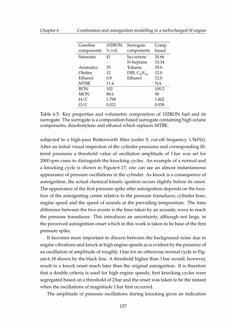
Chapter 6 Combustion and autoignition modelling in a turbocharged SI engine
Gasoline 102RON Surrogate Comp.components % vol. components basedSaturates 41 Iso-octane 30.66
- N-heptane 10.34Aromatics 35 Toluene 35.0Olefins 12 DIB, C8H16 12.0Ethanol 0.8 Ethanol 12.0MTBE 11.4 NARON 102 100.2MON 88.6 90H/C 1.798 1.802O/C 0.021 0.038
Table 6.5: Key properties and volumetric composition of 102RON fuel and itssurrogate. The surrogate is a composition based surrogate containing high octanecomponents; diisobutylene and ethanol which replaces MTBE.
subjected to a high-pass Butterworth filter (order 9, cut-off frequency 1.5kHz).After an initial visual inspection of the cylinder pressures and corresponding fil-tered pressures a threshold value of oscillation amplitude of 1 bar was set for2000 rpm cases to distinguish the knocking cycles. An example of a normal anda knocking cycle is shown in Figure 6.17; one can see an almost instantaneousappearance of pressure oscillations in the cylinder. As knock is a consequence ofautoignition, the actual chemical kinetic ignition occurs slightly before its onset.The appearance of the first pressure spike after autoignition depends on the loca-tion of the autoigniting centre relative to the pressure transducer, cylinder bore,engine speed and the speed of sounds at the prevailing temperature. The timedifference between the two events is the time taken by an acoustic wave to reachthe pressure transducer. This introduces an uncertainty, although not large, inthe perceived autoignition onset which in this work is taken to be base of the firstpressure spike.
It becomes more important to discern between the background noise due toengine vibrations and knock at high engine speeds as is evident by the presence ofan oscillation of amplitude of roughly 1 bar for an otherwise normal cycle in Fig-ure 6.18 shown by the black line. A threshold higher than 1 bar would, however,result in a knock onset much later than the original autoignition. It is thereforethat a double criteria is used for high engine speeds; first knocking cycles weresegregated based on a threshold of 2 bar and the onset was taken to be the instantwhen the oscillations of magnitude 1 bar first occurred.
The amplitude of pressure oscillations during knocking gives an indication
157
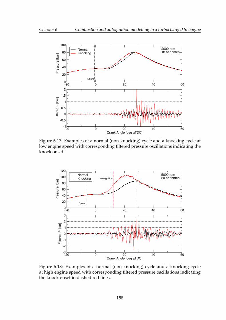
Chapter 6 Combustion and autoignition modelling in a turbocharged SI engine
-20 0 20 40 600
20
40
60
80
100
Pre
ssure
[bar]
NormalKnocking
-20 0 20 40 60Crank Angle [deg aTDC]
-1
-0.5
0
0.5
1
1.5
2
Filt
ere
d P
[bar]
2000 rpm18 bar bmep
Spark
Figure 6.17: Examples of a normal (non-knocking) cycle and a knocking cycle atlow engine speed with corresponding filtered pressure oscillations indicating theknock onset.
-20 0 20 40 600
20
40
60
80
100
120
Pre
ssure
[bar]
NormalKnocking
-20 0 20 40 60Crank Angle [deg aTDC]
-3
-2
-1
0
1
2
3
Filt
ere
d P
[bar]
5000 rpm20 bar bmep
Spark
autoignition
Figure 6.18: Examples of a normal (non-knocking) cycle and a knocking cycleat high engine speed with corresponding filtered pressure oscillations indicatingthe knock onset in dashed red lines.
158
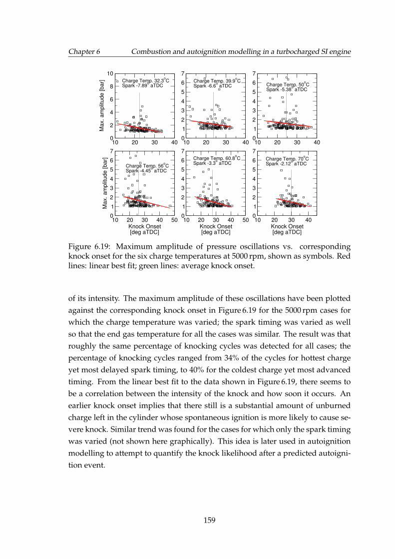
Chapter 6 Combustion and autoignition modelling in a turbocharged SI engine
10 20 30 400
2
4
6
8
10
Max. am
plit
ude [bar]
10 20 30 400
1
2
3
4
5
6
7
10 20 30 400
1
2
3
4
5
6
7
10 20 30 40 50Knock Onset [deg aTDC]
0
1
2
3
4
5
6
7
Max. am
plit
ude [bar]
10 20 30 40 50Knock Onset [deg aTDC]
0
1
2
3
4
5
6
7
10 20 30 40Knock Onset [deg aTDC]
0
1
2
3
4
5
6
7
Charge Temp. 32.3oC
Spark -7.89o aTDC
Charge Temp. 39.9oC
Spark -6.6o aTDC Charge Temp. 50
oC
Spark -5.38o aTDC
Charge Temp. 56oC
Spark -4.45o aTDC
Charge Temp. 60.8oC
Spark -3.3o aTDC
Charge Temp. 70oC
Spark -2.12o aTDC
Figure 6.19: Maximum amplitude of pressure oscillations vs. correspondingknock onset for the six charge temperatures at 5000 rpm, shown as symbols. Redlines: linear best fit; green lines: average knock onset.
of its intensity. The maximum amplitude of these oscillations have been plottedagainst the corresponding knock onset in Figure 6.19 for the 5000 rpm cases forwhich the charge temperature was varied; the spark timing was varied as wellso that the end gas temperature for all the cases was similar. The result was thatroughly the same percentage of knocking cycles was detected for all cases; thepercentage of knocking cycles ranged from 34% of the cycles for hottest chargeyet most delayed spark timing, to 40% for the coldest charge yet most advancedtiming. From the linear best fit to the data shown in Figure 6.19, there seems tobe a correlation between the intensity of the knock and how soon it occurs. Anearlier knock onset implies that there still is a substantial amount of unburnedcharge left in the cylinder whose spontaneous ignition is more likely to cause se-vere knock. Similar trend was found for the cases for which only the spark timingwas varied (not shown here graphically). This idea is later used in autoignitionmodelling to attempt to quantify the knock likelihood after a predicted autoigni-tion event.
159
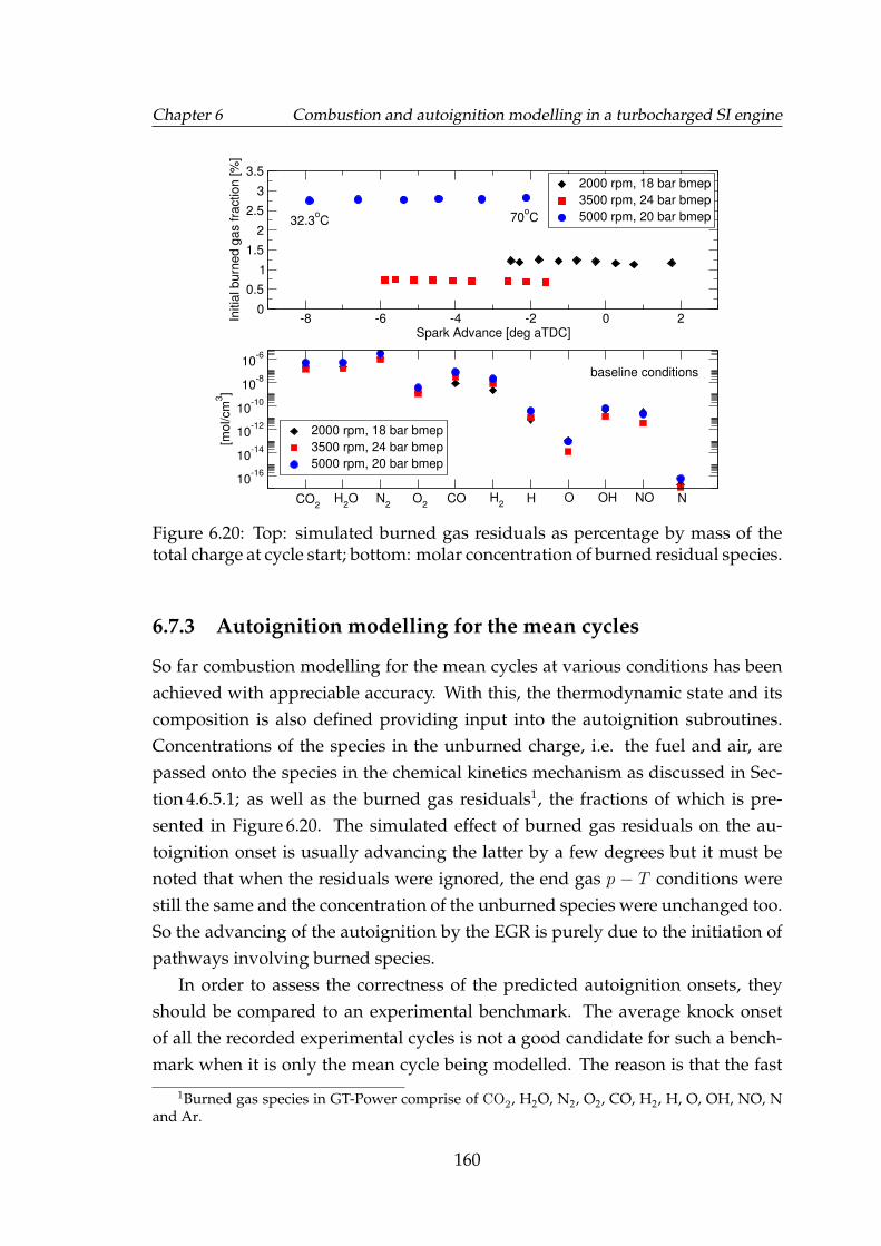
Chapter 6 Combustion and autoignition modelling in a turbocharged SI engine
-8 -6 -4 -2 0 2Spark Advance [deg aTDC]
0
0.5
1
1.5
2
2.5
3
3.5
Initia
l burn
ed g
as fra
ction [%
]
2000 rpm, 18 bar bmep
3500 rpm, 24 bar bmep
5000 rpm, 20 bar bmep
10-16
10-14
10-12
10-10
10-8
10-6
[mol/cm
3]
2000 rpm, 18 bar bmep
3500 rpm, 24 bar bmep
5000 rpm, 20 bar bmep
CO2
H2O
32.3oC 70
oC
N2
O2
CO H2
H O OH NO N
baseline conditions
Figure 6.20: Top: simulated burned gas residuals as percentage by mass of thetotal charge at cycle start; bottom: molar concentration of burned residual species.
6.7.3 Autoignition modelling for the mean cycles
So far combustion modelling for the mean cycles at various conditions has beenachieved with appreciable accuracy. With this, the thermodynamic state and itscomposition is also defined providing input into the autoignition subroutines.Concentrations of the species in the unburned charge, i.e. the fuel and air, arepassed onto the species in the chemical kinetics mechanism as discussed in Sec-tion 4.6.5.1; as well as the burned gas residuals1, the fractions of which is pre-sented in Figure 6.20. The simulated effect of burned gas residuals on the au-toignition onset is usually advancing the latter by a few degrees but it must benoted that when the residuals were ignored, the end gas p − T conditions werestill the same and the concentration of the unburned species were unchanged too.So the advancing of the autoignition by the EGR is purely due to the initiation ofpathways involving burned species.
In order to assess the correctness of the predicted autoignition onsets, theyshould be compared to an experimental benchmark. The average knock onsetof all the recorded experimental cycles is not a good candidate for such a bench-mark when it is only the mean cycle being modelled. The reason is that the fast
1Burned gas species in GT-Power comprise of CO2, H2O, N2, O2, CO, H2, H, O, OH, NO, Nand Ar.
160
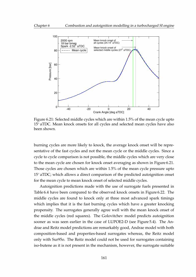
Chapter 6 Combustion and autoignition modelling in a turbocharged SI engine
-40 -20 0 20 40Crank Angle [deg aTDC]
0
20
40
60
80
100
Pre
ssure
[bar]
Mean cycle
2000 rpm18 bar bmepSpark -2.52
o aTDC
Mean knock onset of all cycles (24.14
o aTDC)
Mean knock onset ofselected middle cycles (27
o aTDC)
Figure 6.21: Selected middle cycles which are within 1.5% of the mean cycle upto15◦ aTDC. Mean knock onsets for all cycles and selected mean cycles have alsobeen shown.
burning cycles are more likely to knock, the average knock onset will be repre-sentative of the fast cycles and not the mean cycle or the middle cycles. Since acycle to cycle comparison is not possible, the middle cycles which are very closeto the mean cycle are chosen for knock onset averaging as shown in Figure 6.21.Those cycles are chosen which are within 1.5% of the mean cycle pressure upto15◦ aTDC; which allows a direct comparison of the predicted autoignition onsetfor the mean cycle to mean knock onset of selected middle cycles.
Autoignition predictions made with the use of surrogate fuels presented inTable 6.4 have been compared to the observed knock onsets in Figure 6.22. Themiddle cycles are found to knock only at three most advanced spark timingswhich implies that it is the fast burning cycles which have a greater knockingpropensity. The surrogates generally agree well with the mean knock onset ofthe middle cycles (red squares). The Golovitchev model predicts autoignitionsooner as was seen earlier in the case of LUPOE2-D (see Figure 5.4). The An-drae and Reitz model predictions are remarkably good, Andrae model with bothcomposition-based and properties-based surrogates whereas, the Reitz modelonly with Sur95o. The Reitz model could not be used for surrogates containingiso-butene as it is not present in the mechanism, however, the surrogate suitable
161
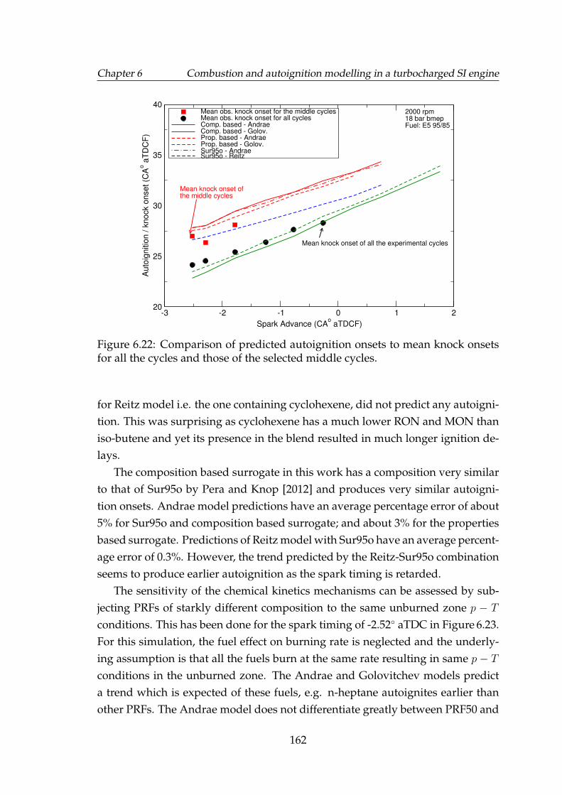
Chapter 6 Combustion and autoignition modelling in a turbocharged SI engine
-3 -2 -1 0 1 2
Spark Advance (CAo aTDCF)
20
25
30
35
40
Auto
ignitio
n / k
nock o
nset (C
Ao a
TD
CF
)
Mean obs. knock onset for the middle cyclesMean obs. knock onset for all cyclesComp. based - AndraeComp. based - Golov.Prop. based - AndraeProp. based - Golov.Sur95o - AndraeSur95o - Reitz
2000 rpm18 bar bmepFuel: E5 95/85
Mean knock onset of all the experimental cycles
Mean knock onset ofthe middle cycles
Figure 6.22: Comparison of predicted autoignition onsets to mean knock onsetsfor all the cycles and those of the selected middle cycles.
for Reitz model i.e. the one containing cyclohexene, did not predict any autoigni-tion. This was surprising as cyclohexene has a much lower RON and MON thaniso-butene and yet its presence in the blend resulted in much longer ignition de-lays.
The composition based surrogate in this work has a composition very similarto that of Sur95o by Pera and Knop [2012] and produces very similar autoigni-tion onsets. Andrae model predictions have an average percentage error of about5% for Sur95o and composition based surrogate; and about 3% for the propertiesbased surrogate. Predictions of Reitz model with Sur95o have an average percent-age error of 0.3%. However, the trend predicted by the Reitz-Sur95o combinationseems to produce earlier autoignition as the spark timing is retarded.
The sensitivity of the chemical kinetics mechanisms can be assessed by sub-jecting PRFs of starkly different composition to the same unburned zone p − T
conditions. This has been done for the spark timing of -2.52◦ aTDC in Figure 6.23.For this simulation, the fuel effect on burning rate is neglected and the underly-ing assumption is that all the fuels burn at the same rate resulting in same p − Tconditions in the unburned zone. The Andrae and Golovitchev models predicta trend which is expected of these fuels, e.g. n-heptane autoignites earlier thanother PRFs. The Andrae model does not differentiate greatly between PRF50 and
162
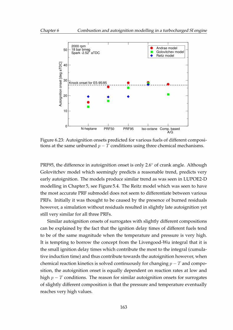
Chapter 6 Combustion and autoignition modelling in a turbocharged SI engine
0
10
20
30
40
50
Auto
ignitio
n o
nset [d
eg a
TD
C]
Andrae modelGolovitchev modelReitz model
2000 rpm18 bar bmepSpark -2.52
o aTDC
Knock onset for E5-95/85
N-heptane Iso-octanePRF95PRF50 Comp. based A/G
Figure 6.23: Autoignition onsets predicted for various fuels of different composi-tions at the same unburned p− T conditions using three chemical mechanisms.
PRF95, the difference in autoignition onset is only 2.6◦ of crank angle. AlthoughGolovitchev model which seemingly predicts a reasonable trend, predicts veryearly autoignition. The models produce similar trend as was seen in LUPOE2-Dmodelling in Chapter 5, see Figure 5.4. The Reitz model which was seen to havethe most accurate PRF submodel does not seem to differentiate between variousPRFs. Initially it was thought to be caused by the presence of burned residualshowever, a simulation without residuals resulted in slightly late autoignition yetstill very similar for all three PRFs.
Similar autoignition onsets of surrogates with slightly different compositionscan be explained by the fact that the ignition delay times of different fuels tendto be of the same magnitude when the temperature and pressure is very high.It is tempting to borrow the concept from the Livengood-Wu integral that it isthe small ignition delay times which contribute the most to the integral (cumula-tive induction time) and thus contribute towards the autoignition however, whenchemical reaction kinetics is solved continuously for changing p− T and compo-sition, the autoignition onset is equally dependent on reaction rates at low andhigh p − T conditions. The reason for similar autoignition onsets for surrogatesof slightly different composition is that the pressure and temperature eventuallyreaches very high values.
163
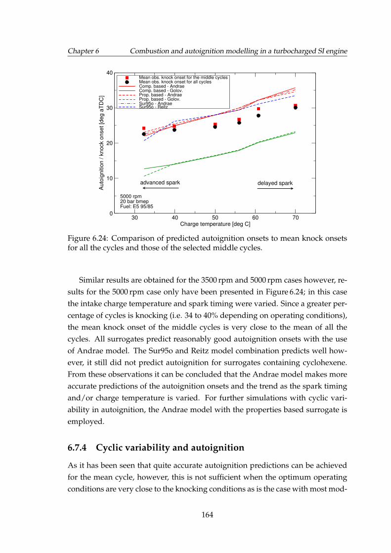
Chapter 6 Combustion and autoignition modelling in a turbocharged SI engine
30 40 50 60 70Charge temperature [deg C]
0
10
20
30
40
Auto
ignitio
n / k
nock o
nset [d
eg a
TD
C]
Mean obs. knock onset for the middle cyclesMean obs. knock onset for all cyclesComp. based - AndraeComp. based - Golov.Prop. based - AndraeProp. based - Golov.Sur95o - AndraeSur95o - Reitz
5000 rpm20 bar bmepFuel: E5 95/85
delayed sparkadvanced spark
Figure 6.24: Comparison of predicted autoignition onsets to mean knock onsetsfor all the cycles and those of the selected middle cycles.
Similar results are obtained for the 3500 rpm and 5000 rpm cases however, re-sults for the 5000 rpm case only have been presented in Figure 6.24; in this casethe intake charge temperature and spark timing were varied. Since a greater per-centage of cycles is knocking (i.e. 34 to 40% depending on operating conditions),the mean knock onset of the middle cycles is very close to the mean of all thecycles. All surrogates predict reasonably good autoignition onsets with the useof Andrae model. The Sur95o and Reitz model combination predicts well how-ever, it still did not predict autoignition for surrogates containing cyclohexene.From these observations it can be concluded that the Andrae model makes moreaccurate predictions of the autoignition onsets and the trend as the spark timingand/or charge temperature is varied. For further simulations with cyclic vari-ability in autoignition, the Andrae model with the properties based surrogate isemployed.
6.7.4 Cyclic variability and autoignition
As it has been seen that quite accurate autoignition predictions can be achievedfor the mean cycle, however, this is not sufficient when the optimum operatingconditions are very close to the knocking conditions as is the case with most mod-
164
Chapter 6 Combustion and autoignition modelling in a turbocharged SI engine
ern engines. In such cases, prediction of a knock-limited spark advance can bebeneficial, particularly during the development phase. Prediction of autoignitionfor the full range of cyclic variability and some means of indicating the severity ofpredicted autoignition can indicate if an operating condition would be infeasible.
The issue of determining whether an autoignition event will lead to knock isof deflagration to detonation transition (DDT) which can be analysed by meansof thermal explosion theories [Radulescu et al., 2013]. However, most of DDTmodels are based on a single step reaction or a double Arrhenius expression toaccount for the two stage heat release. However, such models are fuel specific; inaddition, a spatial resolution of temperature gradient may also be required. Dueto such limitations DDT modelling has not been attempted in this work, however,its inclusion will greatly enhance any future modelling work.
Presently, two knock indices are defined based on various observed relation-ships between knock intensity and engine operating conditions based on the anal-ysis of knock in Di3 engine presented in Section 6.7.2. These can be summarisedas following:
• The detonability of an autoigniting center increases with temperature andpressure.
• The knock intensity is higher when a large portion of charge is still un-burned.
• The knock intensity at same p− T conditions and fraction of unburned fuelyet different engine speeds will be lower at high speeds due to a rapid rateof expansion.
A phenomenological expression based on the above assumptions has beenused for a qualitative appraisal of the knock intensity through a non-dimensionalknock index, KI given as:
KI =606
N(1−mb)e
(−6000Tu
) (6.2)
An arbitrary, experience based threshold value of 5 for the knock index wasfound reasonable in the past for the LUPOE2-D engine which operates at muchlower speeds (up to 3000 rpm when naturally aspirated), however, the knockindex decreases drastically as the engine speed increases (see Figure 6.25b) andthe threshold of 5 does not differentiate between possibly knocking and non-knocking cycles as the knock index becomes smaller than 5 for engine speeds
165
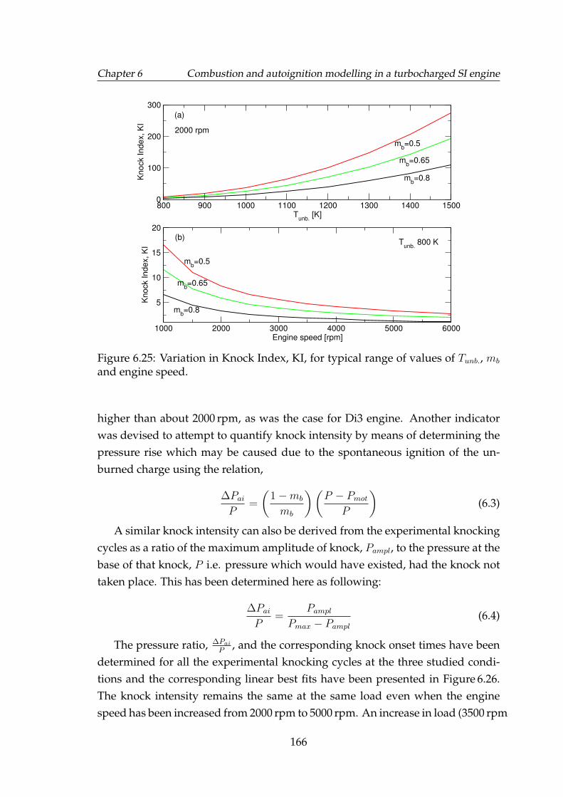
Chapter 6 Combustion and autoignition modelling in a turbocharged SI engine
800 900 1000 1100 1200 1300 1400 1500T
unb. [K]
0
100
200
300
Knock Index, K
I
1000 2000 3000 4000 5000 6000Engine speed [rpm]
5
10
15
20
Knock Index, K
I
mb=0.8
mb=0.5
mb=0.65
mb=0.5
mb=0.65
mb=0.8
2000 rpm
Tunb.
800 K
(a)
(b)
Figure 6.25: Variation in Knock Index, KI, for typical range of values of Tunb., mb
and engine speed.
higher than about 2000 rpm, as was the case for Di3 engine. Another indicatorwas devised to attempt to quantify knock intensity by means of determining thepressure rise which may be caused due to the spontaneous ignition of the un-burned charge using the relation,
∆PaiP
=
(1−mb
mb
)(P − Pmot
P
)(6.3)
A similar knock intensity can also be derived from the experimental knockingcycles as a ratio of the maximum amplitude of knock, Pampl, to the pressure at thebase of that knock, P i.e. pressure which would have existed, had the knock nottaken place. This has been determined here as following:
∆PaiP
=Pampl
Pmax − Pampl(6.4)
The pressure ratio, ∆PaiP
, and the corresponding knock onset times have beendetermined for all the experimental knocking cycles at the three studied condi-tions and the corresponding linear best fits have been presented in Figure 6.26.The knock intensity remains the same at the same load even when the enginespeed has been increased from 2000 rpm to 5000 rpm. An increase in load (3500 rpm
166
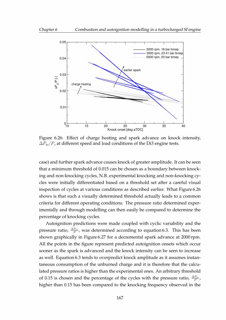
Chapter 6 Combustion and autoignition modelling in a turbocharged SI engine
10 15 20 25 30 35 40Knock onset [deg aTDC]
0
0.01
0.02
0.03
0.04
0.05
∆P
ai/P
[-]
earlier spark
charge heating
2000 rpm, 18 bar bmep
3500 rpm, 23.41 bar bmep
5000 rpm, 20 bar bmep
Figure 6.26: Effect of charge heating and spark advance on knock intensity,∆Pai/P , at different speed and load conditions of the Di3 engine tests.
case) and further spark advance causes knock of greater amplitude. It can be seenthat a minimum threshold of 0.015 can be chosen as a boundary between knock-ing and non-knocking cycles, N.B. experimental knocking and non-knocking cy-cles were initially differentiated based on a threshold set after a careful visualinspection of cycles at various conditions as described earlier. What Figure 6.26shows is that such a visually determined threshold actually leads to a commoncriteria for different operating conditions. The pressure ratio determined exper-imentally and through modelling can then easily be compared to determine thepercentage of knocking cycles.
Autoignition predictions were made coupled with cyclic variability and thepressure ratio, ∆Pai
P, was determined according to equation 6.3. This has been
shown graphically in Figure 6.27 for a decremental spark advance at 2000 rpm.All the points in the figure represent predicted autoignition onsets which occursooner as the spark is advanced and the knock intensity can be seen to increaseas well. Equation 6.3 tends to overpredict knock amplitude as it assumes instan-taneous consumption of the unburned charge and it is therefore that the calcu-lated pressure ratios is higher than the experimental ones. An arbitrary thresholdof 0.15 is chosen and the percentage of the cycles with the pressure ratio, ∆Pai
P,
higher than 0.15 has been compared to the knocking frequency observed in the
167
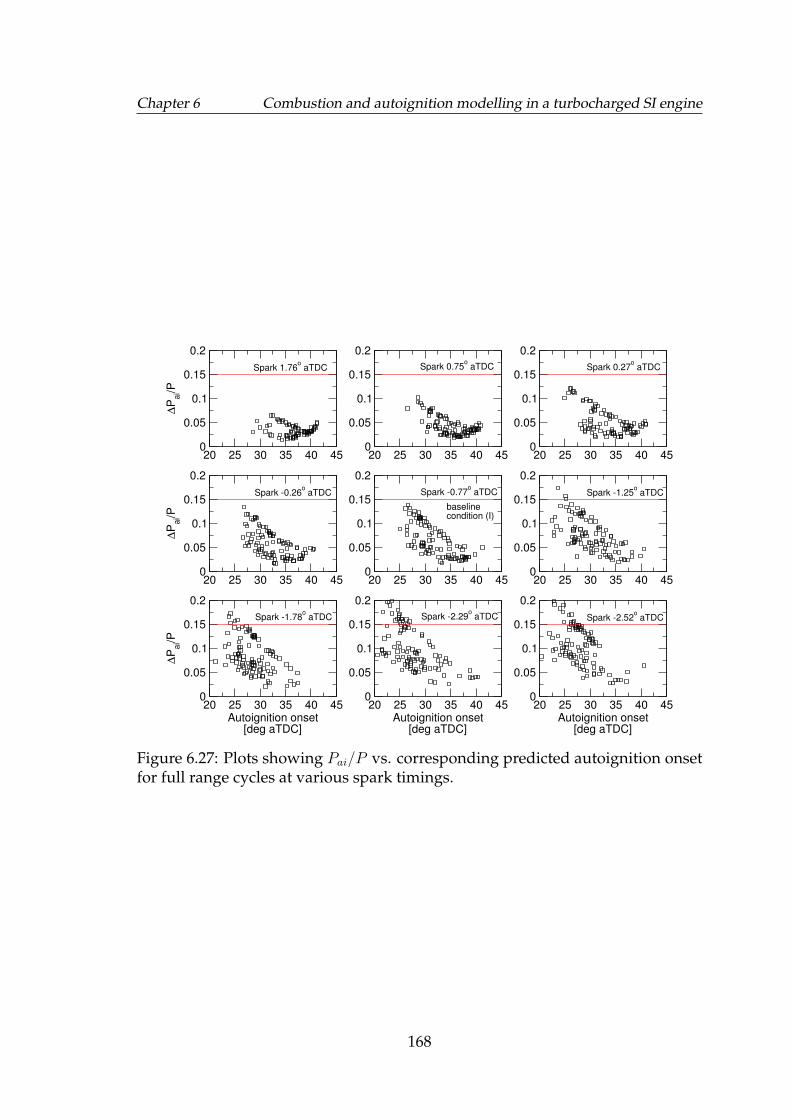
Chapter 6 Combustion and autoignition modelling in a turbocharged SI engine
20 25 30 35 40 450
0.05
0.1
0.15
0.2
∆P
ai/P
20 25 30 35 40 450
0.05
0.1
0.15
0.2
20 25 30 35 40 450
0.05
0.1
0.15
0.2
20 25 30 35 40 450
0.05
0.1
0.15
0.2
∆P
ai/P
20 25 30 35 40 450
0.05
0.1
0.15
0.2
20 25 30 35 40 450
0.05
0.1
0.15
0.2
20 25 30 35 40 45Autoignition onset [deg aTDC]
0
0.05
0.1
0.15
0.2
∆P
ai/P
20 25 30 35 40 45Autoignition onset [deg aTDC]
0
0.05
0.1
0.15
0.2
20 25 30 35 40 45Autoignition onset [deg aTDC]
0
0.05
0.1
0.15
0.2
Spark 1.76o aTDC Spark 0.75
o aTDC Spark 0.27
o aTDC
Spark -0.26o aTDC Spark -0.77
o aTDC Spark -1.25
o aTDC
Spark -2.52o aTDCSpark -2.29
o aTDCSpark -1.78
o aTDC
baselinecondition (I)
Figure 6.27: Plots showing Pai/P vs. corresponding predicted autoignition onsetfor full range cycles at various spark timings.
168
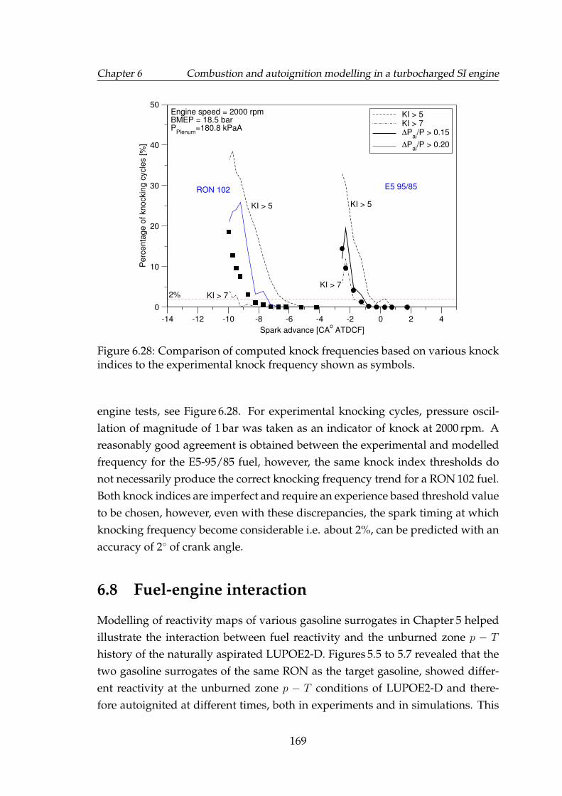
Chapter 6 Combustion and autoignition modelling in a turbocharged SI engine
-14 -12 -10 -8 -6 -4 -2 0 2 4
Spark advance [CAo ATDCF]
0
10
20
30
40
50
Perc
enta
ge o
f knockin
g c
ycle
s [%
]
KI > 5KI > 7∆P
ai/P > 0.15
∆Pai/P > 0.20
Engine speed = 2000 rpmBMEP = 18.5 barP
Plenum=180.8 kPaA
KI > 7
KI > 5KI > 5
KI > 7
E5 95/85RON 102
2%
Figure 6.28: Comparison of computed knock frequencies based on various knockindices to the experimental knock frequency shown as symbols.
engine tests, see Figure 6.28. For experimental knocking cycles, pressure oscil-lation of magnitude of 1 bar was taken as an indicator of knock at 2000 rpm. Areasonably good agreement is obtained between the experimental and modelledfrequency for the E5-95/85 fuel, however, the same knock index thresholds donot necessarily produce the correct knocking frequency trend for a RON 102 fuel.Both knock indices are imperfect and require an experience based threshold valueto be chosen, however, even with these discrepancies, the spark timing at whichknocking frequency become considerable i.e. about 2%, can be predicted with anaccuracy of 2◦ of crank angle.
6.8 Fuel-engine interaction
Modelling of reactivity maps of various gasoline surrogates in Chapter 5 helpedillustrate the interaction between fuel reactivity and the unburned zone p − T
history of the naturally aspirated LUPOE2-D. Figures 5.5 to 5.7 revealed that thetwo gasoline surrogates of the same RON as the target gasoline, showed differ-ent reactivity at the unburned zone p − T conditions of LUPOE2-D and there-fore autoignited at different times, both in experiments and in simulations. This
169
Chapter 6 Combustion and autoignition modelling in a turbocharged SI engine
demonstrated the diminished relevance of RON to autoignition characterisationof fuels in engines different from the CFR engine. This notion is reinforced for aturbocharged engine such as the Di3 engine when the unburned zone p − T his-tories at different conditions of the Di3 engine are plotted, see Figure 6.29 whichalso shows the τign contour map computed for a five-component surrogate for theE5-95/85 gasoline, see the properties-based surrogate in Table 6.4. Two key ob-servations can be made which are that the Di3 engine operates further afar fromthe p − T trajectories of the RON and MON tests shown in Chapter 5. Owingto intercooling, the temperature at any given pressure is lower than that of theLUPOE2-D or the CFR engine. This results in a negative K-value at the three Di3engine conditions as given by Equation 1.3; -1.22 for 2000 rpm and 30 bar bmep,-0.89 for 2000 rpm and 18 bar bmep and -0.72 for 5000 rpm and 20 bar bmep. Thesecond observation is that the gasoline surrogate does not show a NTC behaviourand that for high enough pressures, i.e. higher than 40 bar, the autoignition delaytimes do not seem to be sensitive to pressure change for temperatures upto about750 K. As a result, an increase in load as e.g. at 2000 rpm does not increase thepredicted autoignition propensity, in fact autoignition is predicted at lower loadas p − T trajectory enters shorter ignition delay times when a higher pressuretrajectory stays in longer ignition delay times.
An increase in engine speed increases the K-value, also shown by Kalghatgi[2014] and even though the p− T trajectory passes through regions of short igni-tion delay times, the autoignition onset is much delayed as the times spent by theend gas at these short ignition delay times is smaller.
6.9 General discussion and conclusions
The quasi-dimensional thermodynamic modelling approach, although sensitiveto the inaccuracies of underlying flow-field definition, predicts remarkably wellthe fuel burning rates for different operating conditions after optimisation of theturbulent length scale which governs the burning of eddies entrained into theflame brush. This results in a fast and reliable prediction of cylinder pressurewhen spark timing and intake charge temperature is varied without the need forany further optimisation of the length scale. The combustion models employed inthis work have been applied to their limits in terms of the engine operating con-ditions. Past modelling studies at Leeds University using LUSIE/GT-LU of lowspeed simple geometry engines such as LUPOE, did not require a great deal of
170
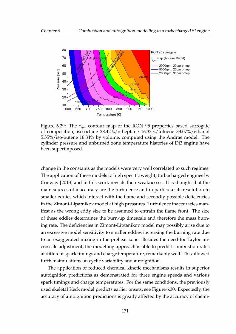
Chapter 6 Combustion and autoignition modelling in a turbocharged SI engine
100ms 50ms 20ms 10ms5.0ms 3.0ms
2.0ms1.5ms
1.0ms
0.50ms
600 650 700 750 800 850 900 950 100010
20
30
40
50
60
70
80
2000rpm, 20bar bmep 5000rpm, 20bar bmep 2000rpm, 30bar bmep
No A
I pre
dicte
d RON 95 surrogate
ign map (Andrae Model)
Temperature [K]
Pres
sure
[bar
]
AI pr
edict
ed m
uch l
ater
AI predicted
Figure 6.29: The τign contour map of the RON 95 properties based surrogateof composition, iso-octane 28.42%/n-heptane 16.33%/toluene 33.07%/ethanol5.35%/iso-butene 16.84% by volume, computed using the Andrae model. Thecylinder pressure and unburned zone temperature histories of Di3 engine havebeen superimposed.
change in the constants as the models were very well correlated to such regimes.The application of these models to high specific weight, turbocharged engines byConway [2013] and in this work reveals their weaknesses. It is thought that themain sources of inaccuracy are the turbulence and in particular its resolution tosmaller eddies which interact with the flame and secondly possible deficienciesin the Zimont-Lipatnikov model at high pressures. Turbulence inaccuracies man-ifest as the wrong eddy size to be assumed to entrain the flame front. The sizeof these eddies determines the burn-up timescale and therefore the mass burn-ing rate. The deficiencies in Zimont-Liptanikov model may possibly arise due toan excessive model sensitivity to smaller eddies increasing the burning rate dueto an exaggerated mixing in the preheat zone. Besides the need for Taylor mi-croscale adjustment, the modelling approach is able to predict combustion ratesat different spark timings and charge temperature, remarkably well. This allowedfurther simulations on cyclic variability and autoignition.
The application of reduced chemical kinetic mechanisms results in superiorautoignition predictions as demonstrated for three engine speeds and variousspark timings and charge temperatures. For the same conditions, the previouslyused skeletal Keck model predicts earlier onsets, see Figure 6.30. Expectedly, theaccuracy of autoignition predictions is greatly affected by the accuracy of chemi-
171
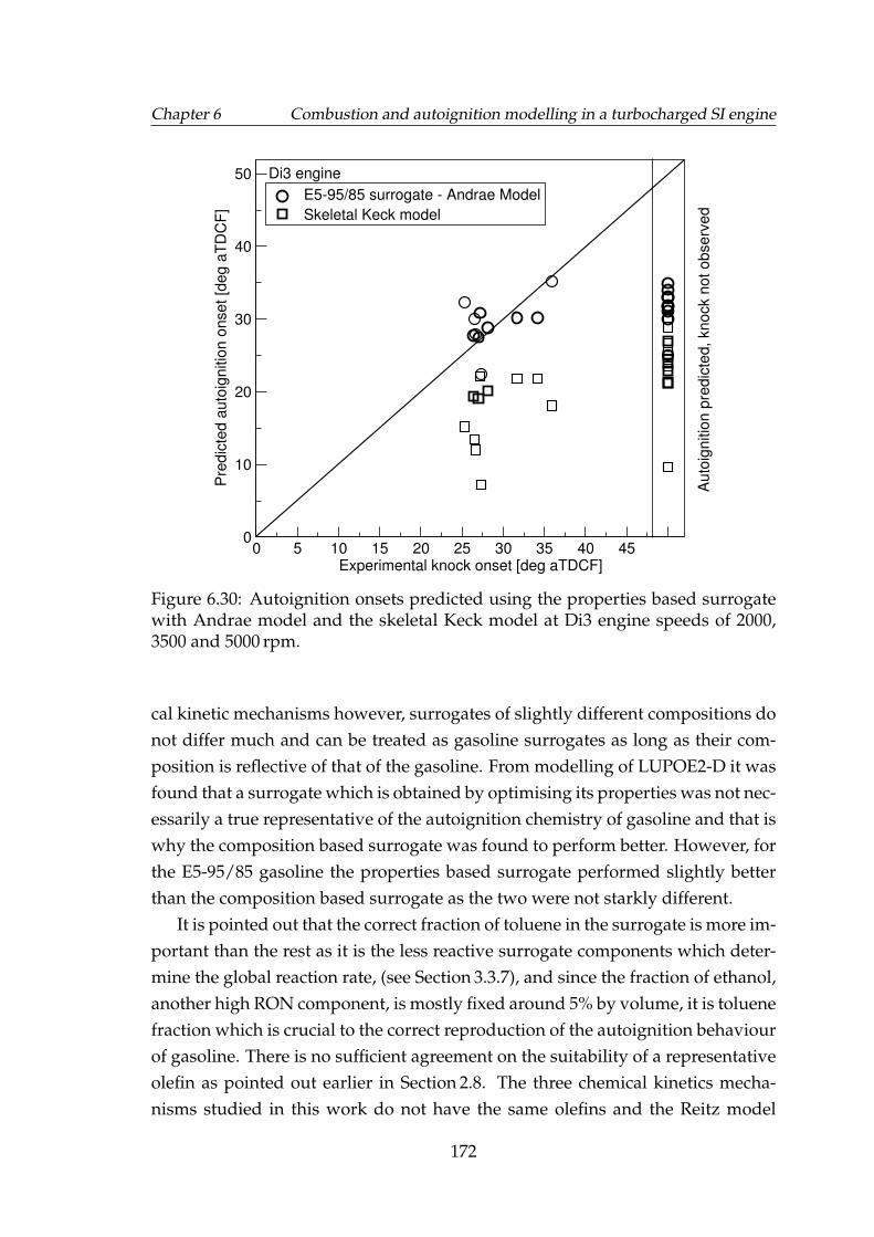
Chapter 6 Combustion and autoignition modelling in a turbocharged SI engine
0 5 10 15 20 25 30 35 40 45Experimental knock onset [deg aTDCF]
0
10
20
30
40
50
Pre
dic
ted a
uto
ignitio
n o
nset [d
eg a
TD
CF
]
E5-95/85 surrogate - Andrae Model
Skeletal Keck model
Auto
ignitio
n p
redic
ted, knock n
ot observ
ed
Di3 engine
Figure 6.30: Autoignition onsets predicted using the properties based surrogatewith Andrae model and the skeletal Keck model at Di3 engine speeds of 2000,3500 and 5000 rpm.
cal kinetic mechanisms however, surrogates of slightly different compositions donot differ much and can be treated as gasoline surrogates as long as their com-position is reflective of that of the gasoline. From modelling of LUPOE2-D it wasfound that a surrogate which is obtained by optimising its properties was not nec-essarily a true representative of the autoignition chemistry of gasoline and that iswhy the composition based surrogate was found to perform better. However, forthe E5-95/85 gasoline the properties based surrogate performed slightly betterthan the composition based surrogate as the two were not starkly different.
It is pointed out that the correct fraction of toluene in the surrogate is more im-portant than the rest as it is the less reactive surrogate components which deter-mine the global reaction rate, (see Section 3.3.7), and since the fraction of ethanol,another high RON component, is mostly fixed around 5% by volume, it is toluenefraction which is crucial to the correct reproduction of the autoignition behaviourof gasoline. There is no sufficient agreement on the suitability of a representativeolefin as pointed out earlier in Section 2.8. The three chemical kinetics mecha-nisms studied in this work do not have the same olefins and the Reitz model
172
Chapter 6 Combustion and autoignition modelling in a turbocharged SI engine
which has one of the more suitable olefins, cyclohexene, predicts excessively longignition delay times with it. It is for this reason that surrogates with olefin havenot performed well in this work. For surrogates containing four components, iso-octane, n-hetpane, toluene and ethanol, the relative proportion of iso-octane andn-heptane can be adjusted to optimise RON and MON. However, the gasolinecomposition analyses presented in [Pera and Knop, 2012], [Bradley and Head,2006] and [Mehl et al., 2011] reveal that the branched to straight chained alkanesratio is approximately 3.5:1. This proportion is used in cases when the compo-sition breakdown of alkanes in the target gasoline is unknown. Surrogates withPRF proportions different from this value do not necessarily produce very dif-ferent autoignition onsets. The properties based surrogate for ULG90 has muchhigher toluene content than the gasoline and too low a cyclohexane fraction tocause longer delays, hence the greater observed difference between the simu-lated and actual autoignition onsets. The surrogates for E5-95/85 have similartoluene content and yet the PRFs and olefin in the surrogates are much different,the autoignition onsets are not so much. This is also partly because the Di3 engineis able to achieve much higher p − T conditions at which the induction times ofdifferent fuels converge to similar values.
To conclude, attempting to optimise a gasoline surrogate with the given levelsof accuracy in chemical kinetic mechanisms and octane number models, is ratheran unproductive endeavour as slight differences in surrogate composition do notcause much difference in autoignition onsets. The chemical kinetics modellingof autoignition will in fact benefit the most through more fundamental researchon the determination and improvement of chemical kinetics for surrogate com-ponents at high pressures. Studies into theoretical octane number models bearsecondary importance as RON and MON have diminished relevance to modernturbocharged engines.
173
Chapter 7
Conclusions and futurerecommendations
7.1 Introduction
This work comprises development of a Fortran code for chemical kinetics calcu-lations of autoignition in the end gas of SI engines (Chapter 2). The code wascombined with an existing quasi-dimensional thermodynamic combustion mod-elling code named LUSIE. The resulting LUSIE code was then coupled with thecommercial packages, GT-Power (Chapter 4). This allowed fast parametric sim-ulations of the engine process allowing to study the effects of different operatingconditions on combustion and autoignition. This was done to address the issueof predictability of autoignition event particularly in turbocharged, downsizedSI engines (Chapters 5 & 6). The use of chemical kinetics also allowed a studyof the interactions of key gasoline surrogate components, iso-octane, n-heptane,toluene and ethanol; during autoignition reactions (Chapter 3).
Key conclusions from the various studies done in this work have been sum-marised in the following section. Recommendations on the further improvementof the tools developed in this work and areas of study are presented as well.
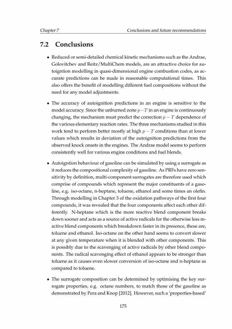
Chapter 7 Conclusions and future recommendations
7.2 Conclusions
• Reduced or semi-detailed chemical kinetic mechanisms such as the Andrae,Golovitchev and Reitz/MultiChem models, are an attractive choice for au-toigntion modelling in quasi-dimensional engine combustion codes, as ac-curate predictions can be made in reasonable computational times. Thisalso offers the benefit of modelling different fuel compositions without theneed for any model adjustments.
• The accuracy of autoignition predictions in an engine is sensitive to themodel accuracy. Since the unburned zone p−T in an engine is continuouslychanging, the mechanism must predict the correction p − T dependence ofthe various elementary reaction rates. The three mechanisms studied in thiswork tend to perform better mostly at high p − T conditions than at lowervalues which results in deviation of the autoignition predictions from theobserved knock onsets in the engines. The Andrae model seems to performconsistently well for various engine conditions and fuel blends.
• Autoigntion behaviour of gasoline can be simulated by using a surrogate asit reduces the compositional complexity of gasoline. As PRFs have zero sen-sitivity by definition, multi-component surrogates are therefore used whichcomprise of compounds which represent the major constituents of a gaso-line, e.g. iso-octane, n-heptane, toluene, ethanol and some times an olefin.Through modelling in Chapter 3 of the oxidation pathways of the first fourcompounds, it was revealed that the four components affect each other dif-ferently. N-heptane which is the more reactive blend component breaksdown sooner and acts as a source of active radicals for the otherwise less re-active blend components which breakdown faster in its presence, these are,toluene and ethanol. Iso-octane on the other hand seems to convert slowerat any given temperature when it is blended with other components. Thisis possibly due to the scavenging of active radicals by other blend compo-nents. The radical scavenging effect of ethanol appears to be stronger thantoluene as it causes even slower conversion of iso-octane and n-heptane ascompared to toluene.
• The surrogate composition can be determined by optimising the key sur-rogate properties, e.g. octane numbers, to match those of the gasoline asdemonstrated by Pera and Knop [2012]. However, such a ‘properties-based’
175
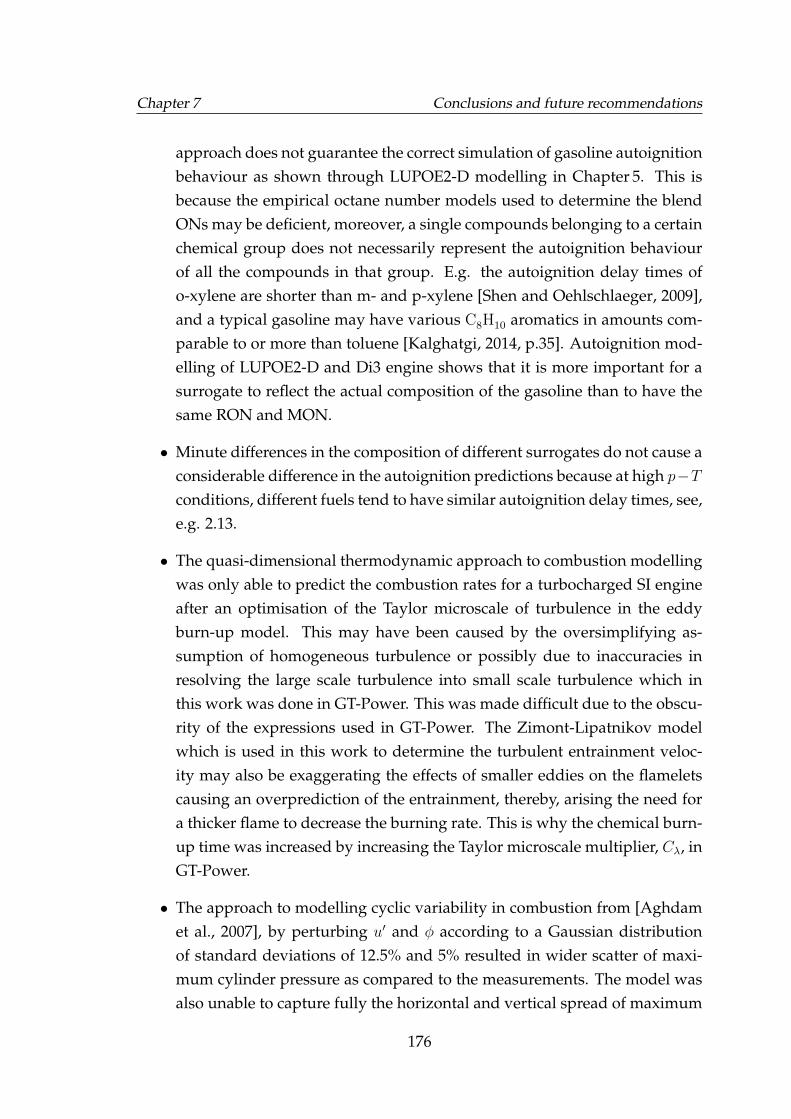
Chapter 7 Conclusions and future recommendations
approach does not guarantee the correct simulation of gasoline autoignitionbehaviour as shown through LUPOE2-D modelling in Chapter 5. This isbecause the empirical octane number models used to determine the blendONs may be deficient, moreover, a single compounds belonging to a certainchemical group does not necessarily represent the autoignition behaviourof all the compounds in that group. E.g. the autoignition delay times ofo-xylene are shorter than m- and p-xylene [Shen and Oehlschlaeger, 2009],and a typical gasoline may have various C8H10 aromatics in amounts com-parable to or more than toluene [Kalghatgi, 2014, p.35]. Autoignition mod-elling of LUPOE2-D and Di3 engine shows that it is more important for asurrogate to reflect the actual composition of the gasoline than to have thesame RON and MON.
• Minute differences in the composition of different surrogates do not cause aconsiderable difference in the autoignition predictions because at high p−Tconditions, different fuels tend to have similar autoignition delay times, see,e.g. 2.13.
• The quasi-dimensional thermodynamic approach to combustion modellingwas only able to predict the combustion rates for a turbocharged SI engineafter an optimisation of the Taylor microscale of turbulence in the eddyburn-up model. This may have been caused by the oversimplifying as-sumption of homogeneous turbulence or possibly due to inaccuracies inresolving the large scale turbulence into small scale turbulence which inthis work was done in GT-Power. This was made difficult due to the obscu-rity of the expressions used in GT-Power. The Zimont-Lipatnikov modelwhich is used in this work to determine the turbulent entrainment veloc-ity may also be exaggerating the effects of smaller eddies on the flameletscausing an overprediction of the entrainment, thereby, arising the need fora thicker flame to decrease the burning rate. This is why the chemical burn-up time was increased by increasing the Taylor microscale multiplier, Cλ, inGT-Power.
• The approach to modelling cyclic variability in combustion from [Aghdamet al., 2007], by perturbing u′ and φ according to a Gaussian distributionof standard deviations of 12.5% and 5% resulted in wider scatter of maxi-mum cylinder pressure as compared to the measurements. The model wasalso unable to capture fully the horizontal and vertical spread of maximum
176
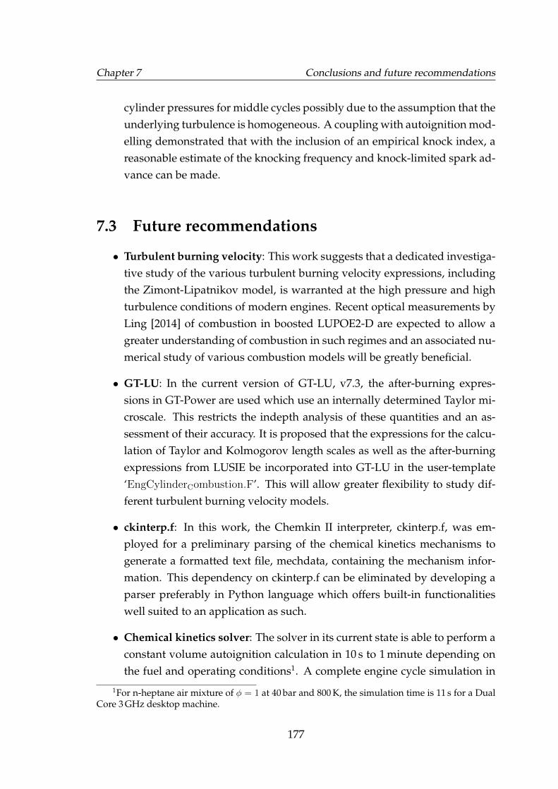
Chapter 7 Conclusions and future recommendations
cylinder pressures for middle cycles possibly due to the assumption that theunderlying turbulence is homogeneous. A coupling with autoignition mod-elling demonstrated that with the inclusion of an empirical knock index, areasonable estimate of the knocking frequency and knock-limited spark ad-vance can be made.
7.3 Future recommendations
• Turbulent burning velocity: This work suggests that a dedicated investiga-tive study of the various turbulent burning velocity expressions, includingthe Zimont-Lipatnikov model, is warranted at the high pressure and highturbulence conditions of modern engines. Recent optical measurements byLing [2014] of combustion in boosted LUPOE2-D are expected to allow agreater understanding of combustion in such regimes and an associated nu-merical study of various combustion models will be greatly beneficial.
• GT-LU: In the current version of GT-LU, v7.3, the after-burning expres-sions in GT-Power are used which use an internally determined Taylor mi-croscale. This restricts the indepth analysis of these quantities and an as-sessment of their accuracy. It is proposed that the expressions for the calcu-lation of Taylor and Kolmogorov length scales as well as the after-burningexpressions from LUSIE be incorporated into GT-LU in the user-template‘EngCylinderCombustion.F’. This will allow greater flexibility to study dif-ferent turbulent burning velocity models.
• ckinterp.f: In this work, the Chemkin II interpreter, ckinterp.f, was em-ployed for a preliminary parsing of the chemical kinetics mechanisms togenerate a formatted text file, mechdata, containing the mechanism infor-mation. This dependency on ckinterp.f can be eliminated by developing aparser preferably in Python language which offers built-in functionalitieswell suited to an application as such.
• Chemical kinetics solver: The solver in its current state is able to perform aconstant volume autoignition calculation in 10 s to 1 minute depending onthe fuel and operating conditions1. A complete engine cycle simulation in
1For n-heptane air mixture of φ = 1 at 40 bar and 800 K, the simulation time is 11 s for a DualCore 3 GHz desktop machine.
177
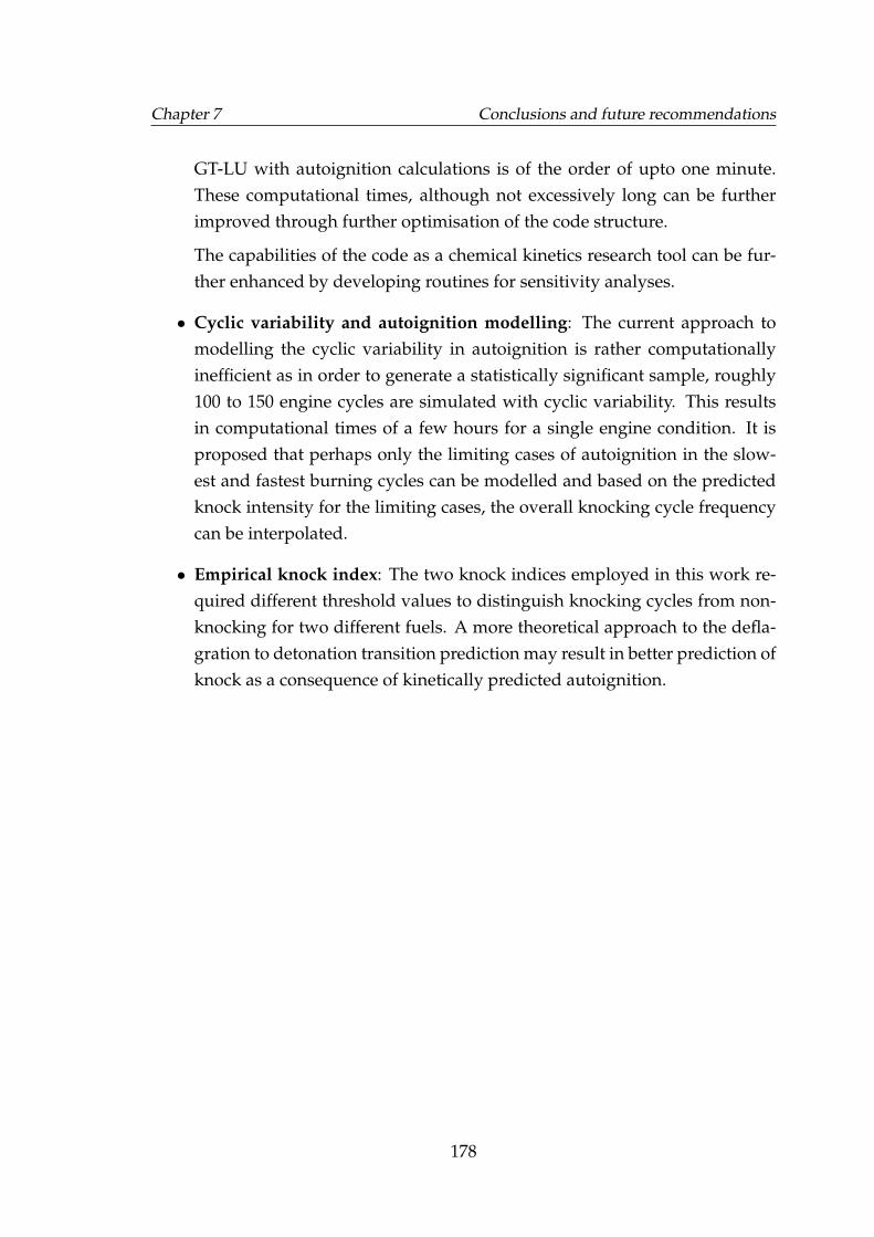
Chapter 7 Conclusions and future recommendations
GT-LU with autoignition calculations is of the order of upto one minute.These computational times, although not excessively long can be furtherimproved through further optimisation of the code structure.
The capabilities of the code as a chemical kinetics research tool can be fur-ther enhanced by developing routines for sensitivity analyses.
• Cyclic variability and autoignition modelling: The current approach tomodelling the cyclic variability in autoignition is rather computationallyinefficient as in order to generate a statistically significant sample, roughly100 to 150 engine cycles are simulated with cyclic variability. This resultsin computational times of a few hours for a single engine condition. It isproposed that perhaps only the limiting cases of autoignition in the slow-est and fastest burning cycles can be modelled and based on the predictedknock intensity for the limiting cases, the overall knocking cycle frequencycan be interpolated.
• Empirical knock index: The two knock indices employed in this work re-quired different threshold values to distinguish knocking cycles from non-knocking for two different fuels. A more theoretical approach to the defla-gration to detonation transition prediction may result in better prediction ofknock as a consequence of kinetically predicted autoignition.
178
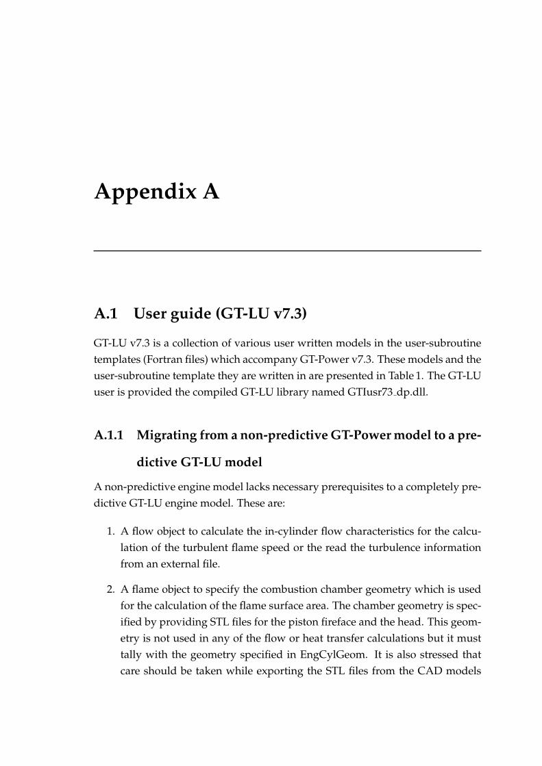
Appendix A
A.1 User guide (GT-LU v7.3)
GT-LU v7.3 is a collection of various user written models in the user-subroutinetemplates (Fortran files) which accompany GT-Power v7.3. These models and theuser-subroutine template they are written in are presented in Table 1. The GT-LUuser is provided the compiled GT-LU library named GTIusr73 dp.dll.
A.1.1 Migrating from a non-predictive GT-Power model to a pre-
dictive GT-LU model
A non-predictive engine model lacks necessary prerequisites to a completely pre-dictive GT-LU engine model. These are:
1. A flow object to calculate the in-cylinder flow characteristics for the calcu-lation of the turbulent flame speed or the read the turbulence informationfrom an external file.
2. A flame object to specify the combustion chamber geometry which is usedfor the calculation of the flame surface area. The chamber geometry is spec-ified by providing STL files for the piston fireface and the head. This geom-etry is not used in any of the flow or heat transfer calculations but it musttally with the geometry specified in EngCylGeom. It is also stressed thatcare should be taken while exporting the STL files from the CAD models
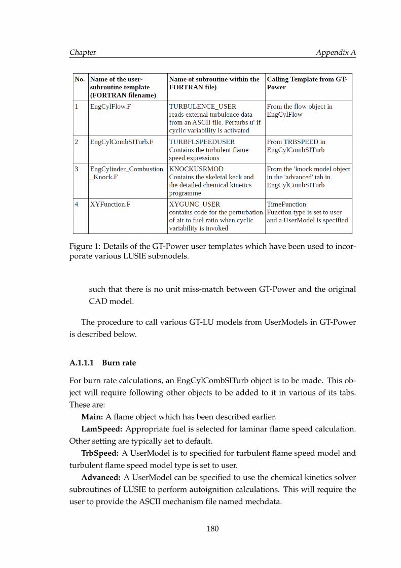
Chapter Appendix A
Figure 1: Details of the GT-Power user templates which have been used to incor-porate various LUSIE submodels.
such that there is no unit miss-match between GT-Power and the originalCAD model.
The procedure to call various GT-LU models from UserModels in GT-Poweris described below.
A.1.1.1 Burn rate
For burn rate calculations, an EngCylCombSITurb object is to be made. This ob-ject will require following other objects to be added to it in various of its tabs.These are:
Main: A flame object which has been described earlier.LamSpeed: Appropriate fuel is selected for laminar flame speed calculation.
Other setting are typically set to default.TrbSpeed: A UserModel is to specified for turbulent flame speed model and
turbulent flame speed model type is set to user.Advanced: A UserModel can be specified to use the chemical kinetics solver
subroutines of LUSIE to perform autoignition calculations. This will require theuser to provide the ASCII mechanism file named mechdata.
180
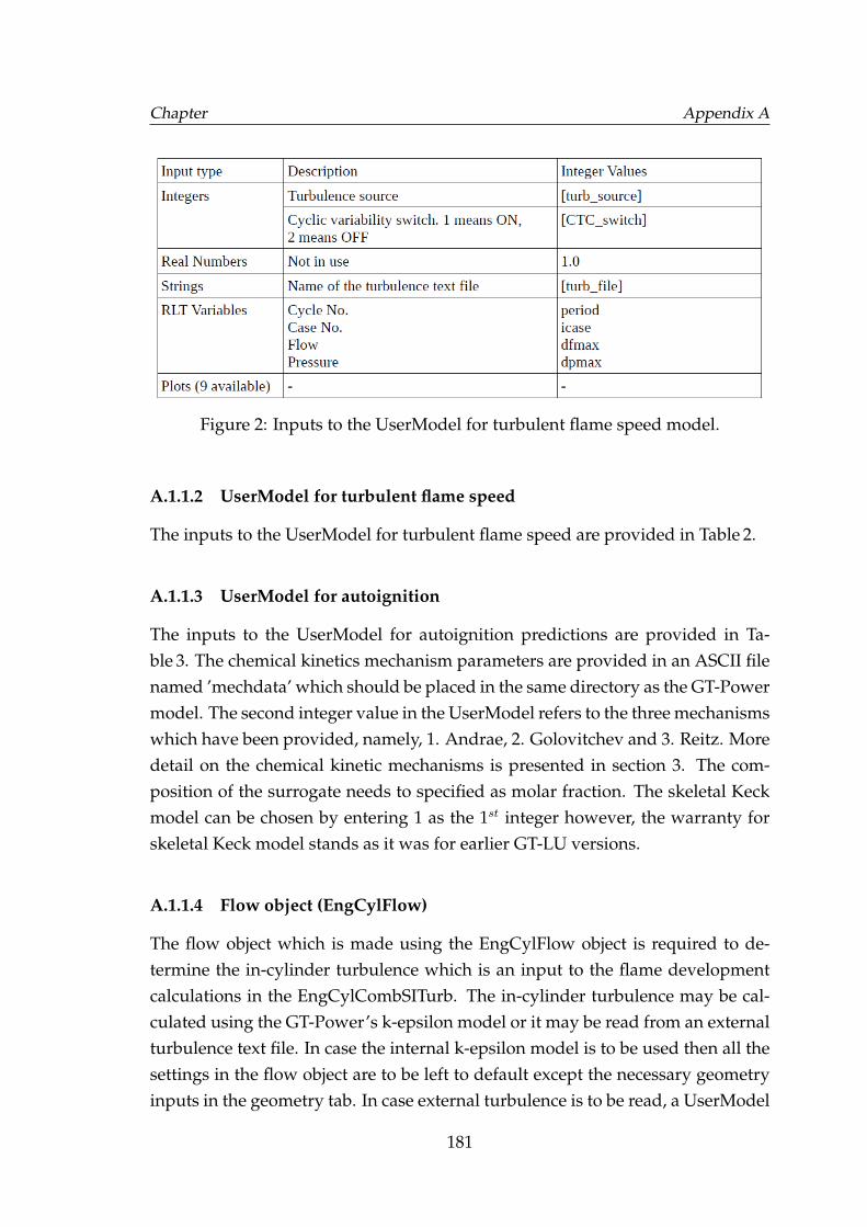
Chapter Appendix A
Figure 2: Inputs to the UserModel for turbulent flame speed model.
A.1.1.2 UserModel for turbulent flame speed
The inputs to the UserModel for turbulent flame speed are provided in Table 2.
A.1.1.3 UserModel for autoignition
The inputs to the UserModel for autoignition predictions are provided in Ta-ble 3. The chemical kinetics mechanism parameters are provided in an ASCII filenamed ’mechdata’ which should be placed in the same directory as the GT-Powermodel. The second integer value in the UserModel refers to the three mechanismswhich have been provided, namely, 1. Andrae, 2. Golovitchev and 3. Reitz. Moredetail on the chemical kinetic mechanisms is presented in section 3. The com-position of the surrogate needs to specified as molar fraction. The skeletal Keckmodel can be chosen by entering 1 as the 1st integer however, the warranty forskeletal Keck model stands as it was for earlier GT-LU versions.
A.1.1.4 Flow object (EngCylFlow)
The flow object which is made using the EngCylFlow object is required to de-termine the in-cylinder turbulence which is an input to the flame developmentcalculations in the EngCylCombSITurb. The in-cylinder turbulence may be cal-culated using the GT-Power’s k-epsilon model or it may be read from an externalturbulence text file. In case the internal k-epsilon model is to be used then all thesettings in the flow object are to be left to default except the necessary geometryinputs in the geometry tab. In case external turbulence is to be read, a UserModel
181
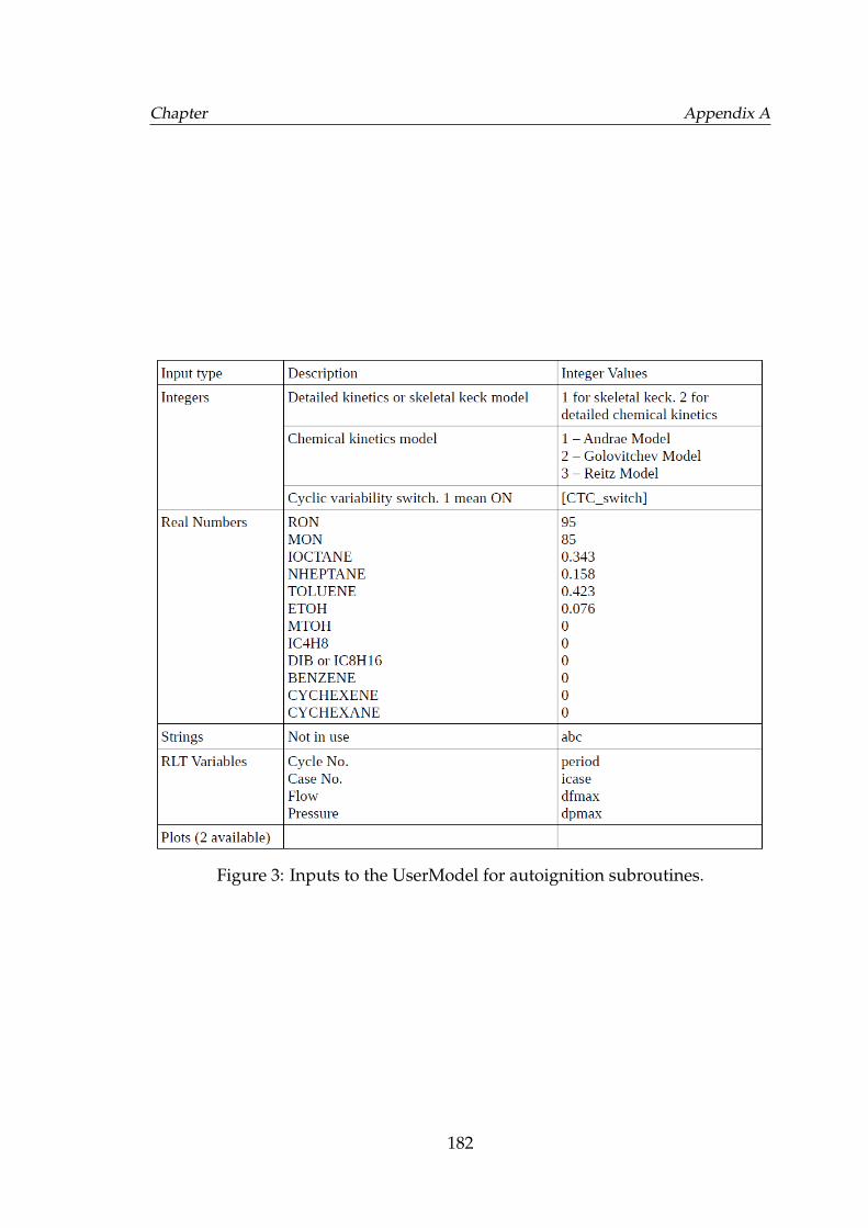
Chapter Appendix A
Figure 3: Inputs to the UserModel for autoignition subroutines.
182
Chapter Appendix A
object is to be made and called from the User Routine tab. Since GT-LU readsonly the in-cylinder root-mean-square velocity (u′) and the integral length scale(L), the flow model type needs to be set to use:trb. The inputs to the UserModelare provided in the following table.
A.1.2 External turbulence file format
An ASCII file containing the in-cylinder rms velocity and integral length scale inSI units must be provided in the same directory as the GT-Power model. The fileshould be structured such that the crank angles are in 1st column, rms velocity in2nd and the integral length scale in 3rd with spaces as delimiters. The format isshown below as an example.
-179.5 9.0344995323 0.0116081259-178.5 8.9840826669 0.011727627-177.5 8.9161701618 0.0118287205... ... ...The total number of data points (rows) must not be more than 2000. A file
larger than 2000 rows would result in a run-time error. Although GT-LU flowsubroutine is able to adjust for a non-zero TDCF but it is highly recommendedto format/adjust the crank angle in the turbulence text file from either -360◦ to+360◦ or -180◦ to +180◦ depending on whether the engine is 4 stroke or 2 stroke,with TDCF at 0◦.
A.1.3 Chemical kinetic mechanisms
GTLU v7.3 offers a provision of the use of three semi-detailed chemical kineticmechanisms which have been discussed in Chapter 2. Each mechanism com-prises of atleast four key surrogate compounds for gasoline namely, iso-octane,n-heptane, toluene and ethanol. Care should be taken while entering the compo-sition of the surrogate in the real numbers tab of the userknock object (UserModelfor autoignition). The RON and MON specified in the real numbers tab of theuserknock are only needed by the older skeletal Keck model and are irrelevant tothe detailed chemistry solver.
183
Chapter Appendix A
A.1.4 Cyclic variability in GT-LU
GT-LU cyclic variability is based on a Gaussian perturbation of the in-cylinderrms velocity and equivalence ratio from one cycle to another. Through researchon the Leeds University ported engines and various other production engine,it has been found that a standard deviation of 12.5% for the rms velocity and avalue of 5% for the equivalence ratio produces a realistic spread in the in-cylinderpressure about its mean value. The GT-LU cyclic variability is designed to workin such a way that when invoked, each case in the GT-Power model will run fora pre-set number of cycles. The in-cylinder pressures for only those cycles willbe written which converge based on the minimization of the mass flow rates andpressures from one cycle to another cycle. The in-cylinder pressures are writtenin text files which are named in a format as e.g. CTC CYLP01 1. Where CTCmean ’cycle to cycle’, CYLP01 means ’cylinder number 1’ and the integer at theend refers to the case number. The cyclic variability parameters are also writtenin a file named CTC METRICS which contains the numbers of the cycles whichare perturbed and also the multipliers for the rms velocity and the equivalenceratio. The metrics for each case are separated by a header.
A.1.4.1 Setting cyclic variability in a GT-LU model
The steps to setting up cyclic variability are given as follows:STEP 1 (The cyclic variability switch) The universal integer switch for cyclic
variability is to be entered in all four UserModels i.e. the userturbspeed, user-knock, the UserModel in the flow object and UserModel in the TimeFunctionwhich is described subsequently. An integer value of 1 means that the cyclic vari-ability is invoked and any value other than 1 would turn off the cyclic variability.
STEP 2 (Time function for air to fuel ratio) A ’TimeFunction’ object needs tobe created to invoke cyclic variability for the equivalence ratio or the air to fuelratio. A UserModel is to be specified in user model object name whose inputsare provided in Table 4. All the other inputs in the TimeFunction should be set to‘ign’. When the TimeFunction is made correctly and called from ’Fuel Ratio’ inthe ’Rate’ tab of the injectors, a run-time message should appear indicating:
GTLU v7.3 - AFR perturbed
184
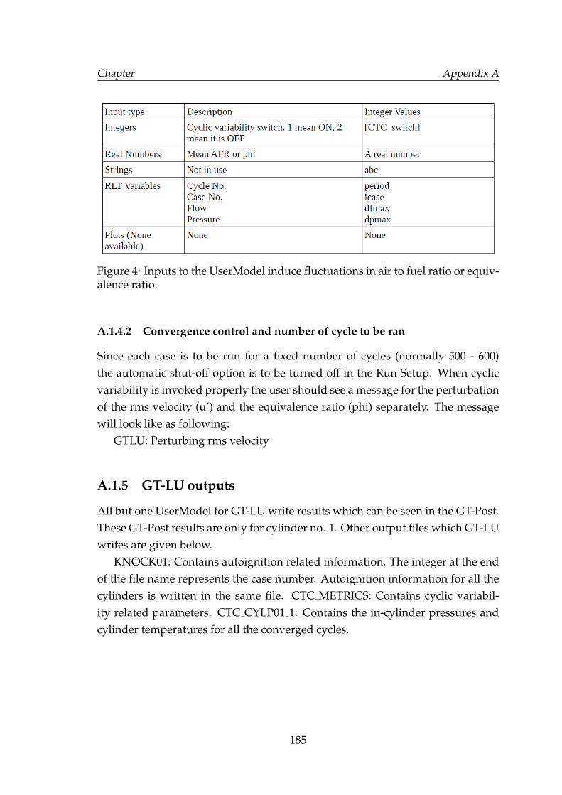
Chapter Appendix A
Figure 4: Inputs to the UserModel induce fluctuations in air to fuel ratio or equiv-alence ratio.
A.1.4.2 Convergence control and number of cycle to be ran
Since each case is to be run for a fixed number of cycles (normally 500 - 600)the automatic shut-off option is to be turned off in the Run Setup. When cyclicvariability is invoked properly the user should see a message for the perturbationof the rms velocity (u’) and the equivalence ratio (phi) separately. The messagewill look like as following:
GTLU: Perturbing rms velocity
A.1.5 GT-LU outputs
All but one UserModel for GT-LU write results which can be seen in the GT-Post.These GT-Post results are only for cylinder no. 1. Other output files which GT-LUwrites are given below.
KNOCK01: Contains autoignition related information. The integer at the endof the file name represents the case number. Autoignition information for all thecylinders is written in the same file. CTC METRICS: Contains cyclic variabil-ity related parameters. CTC CYLP01 1: Contains the in-cylinder pressures andcylinder temperatures for all the converged cycles.
185
References
Abdel-Gayed, R. G., Bradley, D., and Lawes, M. (1987). Turbulent burning veloc-ities: A general correlation in terms of straining rates. Proceedings of the RoyalSociety of London. A. Mathematical and Physical Sciences, 414:389–413.
Abdi Aghdam, E. (2003). Improvement and validation of a thermodynamic S.I. enginesimulation code. PhD thesis, School of Mechanical Engineering, The Universityof Leeds.
Aghdam, A. E., Burluka, A. A., Hattrell, T., Liu, K., Sheppard, C. G. W., Neumeis-ter, J., and Crundwell, N. (2007). Study of cyclic variation in an SI engine usinga quasi-dimensional combustion model. Society of Automotive Engineers, SAETechnical Paper 2007-01-0939.
Al-Mughanam, T. (2013). Fundamental characterisation of the flame propagation ofsynthetic fuels. PhD thesis, School of Mechanical Engineering, The Universityof Leeds.
Anderson, J. E., Kramer, U., Mueller, S. A., and Wallington, T. J. (2010). Octanenumbers of ethanol and methanolgasoline blends estimated from molar con-centrations. Energy & Fuels, 24(12):6576–6585.
Andrae, J. (2008). Development of a detailed kinetic model for gasoline surrogatefuels. Fuel, 87(1011):2013 – 2022.
Andrae, J., Bjrnbom, P., Cracknell, R., and Kalghatgi, G. (2007). Autoignitionof toluene reference fuels at high pressures modeled with detailed chemicalkinetics. Combustion and Flame, 149(12):2 – 24.
Andrae, J. and Head, R. (2009). HCCI experiments with gasoline surrogate fu-els modeled by a semidetailed chemical kinetic model. Combustion and Flame,156(4):842 – 851.
186
REFERENCES
Annand, W. J. D. (1963). Heat transfer in the cylinders of reciprocating inter-nal combustion engines. Proceedings of the Institution of Mechanical Engineers,177(1):973–996.
Attard, W. P., Toulson, E., Watson, H., and Hamori, F. (2010). Abnormal com-bustion including mega knock in a 60turbocharged pfi engine. SAE TechnicalPaper 2010-01-1456.
Barnard, J. and Ibberson, V. (1965). The gaseous oxidation of toluene {II} theanalytical results. Combustion and Flame, 9(2):149 – 157.
Bedoya, I. D., Cadavid, F., Saxena, S., Dibble, R., Aceves, S., and Flowers, D.(2012). A sequential chemical kinetics-cfd-chemical kinetics methodology topredict hcci combustion and main emissions.
Blizard, N. C. and Keck, J. C. (1974). Experimental and theoretical investigationof turbulent burning model for internal combustion engines. SAE Paper No.740191.
Borghi, R. and Destriau, M. (1998). Combustion and flames: chemical and physicalprinciples. Editions Technip, Paris, 1st edition.
Borghi, R., Mura, A., and Burluka, A. A. (2008). Turbulent premixed flames:Experimental studies over last decades. Combustion phenomena, CRC Press.
Bounaceur, R., Da Costa, I., Fournet, R., Billaud, F., and Battin-Leclerc, F. (2005).Experimental and modeling study of the oxidation of toluene. InternationalJournal of Chemical Kinetics, 37(1):25–49.
Bozza, F., Siano, D., and Torella, E. (2009). Cycle-by-cycle analysis, knock mod-eling and spark-advance setting of a downsized spark-ignition turbochargedengine. SAE Int. J. Engines, 2:381–389.
Bradley, D. (1992). How fast can we burn? Symposium (International) onCombustion, 24(1):247 – 262. ¡ce:title¿Twenty-Fourth Symposium on Combus-tion¡/ce:title¿.
Bradley, D. and Head, R. (2006). Engine autoignition: The relationship betweenoctane numbers and autoignition delay times. Combustion and Flame, 147(3):171– 184.
187
REFERENCES
Bradley, D., Lau, A. K. C., and Lawes, M. (1992). Flame stretch rate as a determi-nant of turbulent burning velocity. Philosophical Transactions of the Royal Society: Physical and Engineering Sciences, 338(1650):359–387.
Brezinsky, K. (1986). The high-temperature oxidation of aromatic hydrocarbons.Progress in Energy and Combustion Science, 12(1):1 – 24.
Burgoyne, J. H. (1940). The combustion of aromatic and alicyclic hydrocarbons.v. the products of combustion of benzene and its monoalkyl derivatives. Pro-ceedings of the Royal Society of London. Series A. Mathematical and Physical Sciences,175(963):539–563.
Burluka, A. (2010). Combustion in a spark ignition engine. Handbook of Combus-tion, Volume 3: Gaseous and Liquid Fuels.
Burluka, A., Hussin, A. E.-D., Ling, Z.-Y., and Sheppard, C. (2012). Effects oflarge-scale turbulence on cyclic variability in spark-ignition engine. Experimen-tal Thermal and Fluid Science, 43(0):13 – 22. Seventh Mediterranean CombustionSymposium.
Burluka, A. A., Liu, K., Sheppard, C., Smallbone, A. J., and Woolley, R. (2004).The influence of simulated residual and no concentrations on knock onset forprfs and gasolines.
Cancino, L., Fikri, M., Oliveira, A., and Schulz, C. (2009). Autoignition of gaso-line surrogate mixtures at intermediate temperatures and high pressures: Ex-perimental and numerical approaches. Proceedings of the Combustion Institute,32(1):501 – 508.
Cancino, L., Fikri, M., Oliveira, A., and Schulz, C. (2011). Ignition delay times ofethanol-containing multi-component gasoline surrogates: Shock-tube experi-ments and detailed modeling. Fuel, 90(3):1238 – 1244.
Cancino, L. R., Fikri, M., Oliveira, A. A. M., and Schulz, C. (2010). Measure-ment and chemical kinetics modeling of shock-induced ignition of ethanolairmixtures. Energy & Fuels, 24(5):2830–2840.
Cash, J. (1983). The integration of stiff initial value problems in odes using mod-ified extended backward differentiation formulae. Computers & Mathematicswith Applications, 9(5):645 – 657.
188
REFERENCES
Chun, K. M., Heywood, J. B., and Keck, J. C. (1989). Prediction of knock oc-currence in a spark-ignition engine. Symposium (International) on Combustion,22(1):455 – 463.
Ciezki, H. and Adomeit, G. (1993). Shock-tube investigation of self-ignition of n-heptane-air mixtures under engine relevant conditions. Combustion and Flame,93(4):421 – 433.
Conway, G. T. (2013). Cyclic variability of flame propagation and autoignition in su-percharged and naturally aspirated SI engines. PhD thesis, School of MechanicalEngineering, The University of Leeds.
Cowart, J., Keck, J., Heywood, J., Westbrook, C., and Pitz, W. (1991). Engine knockpredictions using a fully-detailed and a reduced chemical kinetic mechanism.Symposium (International) on Combustion, 23(1):1055 – 1062. ¡ce:title¿Twenty-Third Symposium (International) on Combustion¡/ce:title¿.
Cox, R. and Cole, J. (1985). Chemical aspects of the autoignition of hydrocar-bonair mixtures. Combustion and Flame, 60(2):109 – 123.
Curran, H., Gaffuri, P., Pitz, W., and Westbrook, C. (1998a). A comprehensivemodeling study of n-heptane oxidation. Combustion and Flame, 114(12):149 –177.
Curran, H., Gaffuri, P., Pitz, W., and Westbrook, C. (2002). A comprehensivemodeling study of iso-octane oxidation. Combustion and Flame, 129(3):253 –280.
Curran, H., Pitz, W., Westbrook, C., Callahan, G., and Dryer, F. (1998b). Oxida-tion of automotive primary reference fuels at elevated pressures. Symposium(International) on Combustion, 27(1):379 – 387. Twenty-Seventh Sysposium (In-ternational) on Combustion Volume One.
Dahnz, C. and Spicher, U. (2010). Irregular combustion in supercharged sparkignition engines pre-ignition and other phenomena. International Journal ofEngine Research, 11(6):485–498.
Damkohler, G. (1940). Der einfluss der turbulenz auf die flam-mengeschwindigkeit in gasgemischen. Z Elecktrochem, 46:601.
189
REFERENCES
Darrieus, G. (1938). Propagation d’un front de flamme: Assai de theorie desvitesses anomalies de deflagration par developpment spantane de la turbulen-cel. Presented at the 6th int. Cong. Appl. Mech., Paris.
Davidson, D., Gauthier, B., and Hanson, R. (2005). Shock tube ignition measure-ments of iso-octane/air and toluene/air at high pressures. Proceedings of theCombustion Institute, 30(1):1175 – 1182.
Douaud, A. M. and Eyzat, P. (1978). Four-octane-number method for predictingthe anti-knock behaviour of fuels and engines. Society of Automotive Engineers,SAE Technical Paper 780080.
Farrell, J. and Bunting, B. (2006). Fuel composition effects at constant RON andMON in an HCCI engine operated with negative valve overlap. SAE TechnicalPaper 2006-01-3275.
Fernandes, R. (2010). Combustion chemistry. Handbook of Combustion, Volume 3:Gaseous and Liquid Fuels.
Fieweger, K., Blumenthal, R., and Adomeit, G. (1997). Self-ignition of s.i. enginemodel fuels: A shock tube investigation at high pressure. Combustion and Flame,109(4):599 – 619.
Fikri, M., Herzler, J., Starke, R., Schulz, C., Roth, P., and Kalghatgi, G. (2008).Autoignition of gasoline surrogates mixtures at intermediate temperatures andhigh pressures. Combustion and Flame, 152(12):276 – 281.
Foong, T. M., Morganti, K. J., Brear, M. J., da Silva, G., Yang, Y., and Dryer, F. L.(2014). The octane numbers of ethanol blended with gasoline and its surro-gates. Fuel, 115(0):727 – 739.
Gardiner, W. (2000). Gas-Phase Combustion Chemistry. Springer-Verlag New York,Inc.
Gauthier, B., Davidson, D., and Hanson, R. (2004). Shock tube determination ofignition delay times in full-blend and surrogate fuel mixtures. Combustion andFlame, 139(4):300 – 311.
Ghojel, J. (2010). Review of the development and applications of the wiebe func-tion: A tribute to the contribution of ivan wiebe to engine research. InternationalJournal of Engine Research, 11(4):297–312. cited By (since 1996)14.
190
REFERENCES
Ghosh, P., Hickey, K., and Jaffe, S. (2006). Development of a detailed gasolinecomposition-based octane model. Industrial & Engineering Chemistry Research,45(1):337–345.
Gillespie, L., Lawes, M., Sheppard, C. G. W., and Woolley, R. (2000). Aspects oflaminar and turbulent burning velocity relevant to SI engines. SAE TechnicalPaper 2000-01-0192.
Gordon, S. and BcBride, B. (1971). Computer Program for Calculation of Com-plex Chemical Equilibrium Compositions, Rocket Performance, Incident and ReflectedShocks and Chapman-Jouguet Detonations, NASA SP-273.
Griffiths, J. (1995). Reduced kinetic models and their application to practical com-bustion systems. Progress in Energy and Combustion Science, 21(1):25 – 107.
Griffiths, J. and Mohamed, C. (1997). Chapter 6: Experimental and numeri-cal studies of oxidation chemistry and spontaneous ignition phenomena. InPilling, M., editor, Low-Temperature Combustion and Autoignition, volume 35 ofComprehensive Chemical Kinetics, pages 545 – 660. Elsevier.
Griffiths, J. F. and Barnard, J. A. (1995). Flame and Combustion. Blackie Academic& Professional.
Halstead, M., Kirsch, L., and Quinn, C. (1977). The autoignition of hydrocarbonfuels at high temperatures and pressuresfitting of a mathematical model. Com-bustion and Flame, 30(0):45 – 60.
Han, D., Han, S.-K., Han, B.-H., and Kim, W.-T. (2007). Development of 2.0l tur-bocharged disi engine for downsizing application. SAE Technical Paper 2007-01-0259.
Hartmann, M., Gushterova, I., Fikri, M., Schulz, C., Schiel, R., and Maas, U.(2011). Auto-ignition of toluene-doped n-heptane and iso-octane/air mixtures:High-pressure shock-tube experiments and kinetics modeling. Combustion andFlame, 158(1):172 – 178.
Hattrell, T. (2007). A computational and experimental study of spark ignition combus-tion. PhD thesis, School of Mechanical Engineering, The University of Leeds.
Hattrell, T., Sheppard, C. G. W., Burluka, A. A., Neumeister, J., and Cairns, A.(2006). Burn rate implications of alternative knock reduction strategies for tur-bocharged si engines. SAE Technical Paper 2006-01-1110.
191
REFERENCES
H.E.Avery (1974). Basic Reaction Kinetics and Mechanisms. MacMillan EduationLtd.
Heywood, J. (1988). Internal combustion engine fundamentals. McGraw-Hill, Inc.
Hinze, P. C. and Miles, P. C. (1999). Quantitative measurements of residual andfresh charge mixing in a modern si engine using spontaneous raman scattering.SAE Technical Paper 1999-01-1106.
Hoepke, B., Jannsen, S., Kasseris, E., and Cheng, W. K. (2012). EGR effects onboosted SI engine operation and knock integral correlation. SAE Int. J. Engines,5:547–559.
Hu, H. and Keck, J. (1987). Autoignition of adiabatically compressed combustiblegas mixtures. SAE Technical Paper 872110.
Huang, C., Golovitchev, V., and Lipatnikov, A. (2010). Chemical model ofgasoline-ethanol blends for internal combustion engine applications. SAETechnical Paper 2010-01-0543.
Hussin, A. E. (2012). New and Renewable Energy: Renewable Fuels in Internal Com-bustion Engines. PhD thesis, School of Mechanical Engineering, The Universityof Leeds.
Hynes, J. (1986). A Computational and Experimental Study of Spark Ignition Com-bustion. PhD thesis, Department of Mechanical Engineering, The University ofLeeds.
Jia, M. and Xie, M. (2006). A chemical kinetics model of iso-octane oxidation for{HCCI} engines. Fuel, 85(1718):2593 – 2604.
Johansson, B. (1996). Cycle to cycle variations in s.i. engines - the effects of fluidflow and gas composition in the vicinity of the spark plug on early combustion.SAE Technical Paper 962084.
Kalghatgi, G. (2001). Fuel anti-knock quality - part i. engine studies. SAE Techni-cal Paper 2001-01-3584.
Kalghatgi, G. (2014). Fuel/Engine Interactions. SAE International. DOI 10.4271/R-409.
192
REFERENCES
Knop, V., Loos, M., Pera, C., and Jeuland, N. (2014). A linear-by-mole blend-ing rule for octane numbers of n-heptane/iso-octane/toluene mixtures. Fuel,115(0):666 – 673.
Knop, V., Pera, C., and Duffour, F. (2013). Validation of a ternary gasoline surro-gate in a CAI engine. Combustion and Flame, 160(10):2067 – 2082.
Knox, J. (1967). Photochemistry and Reaction Kinetics. Cambridge University Press.
Koert, D., Miller, D., and Cernansky, N. (1994). Experimental studies of propaneoxidation through the negative temperature coefficient region at 10 and 15 at-mospheres. Combustion and Flame, 96(12):34 – 49.
Kolaitis, D. I. and Founti, M. A. (2010). Cool flames. Handbook of Combustion,Volume 1: Fundamentals and Safety (2010) WILEY-VCH Verlag GmbH & Co.KGaA.
Kolmogorov, A. N. (1941). English translation (1991): The local structure of tur-bulence in incompressible viscous fluid for very large reynolds numbers. Pro-ceedings: Mathematical and Physical Sciences, 434(1890):pp. 9–13.
Kukkadapu, G., Kumar, K., Sung, C.-J., Mehl, M., and Pitz, W. J. (2013). Autoigni-tion of gasoline and its surrogates in a rapid compression machine. Proceedingsof the Combustion Institute, 34(1):345 – 352.
Landau, L. D. (1944). On the theory of slow combustion. Acta Physiochim URSS,90:77–85.
Lenhert, D. B., Miller, D. L., Cernansky, N. P., and Owens, K. G. (2009). Theoxidation of a gasoline surrogate in the negative temperature coefficient region.Combustion and Flame, 156(3):549 – 564.
Leppard, W. R. (1990). The chemical origin of fuel octane sensitivity.
Lewis, B. and von Elbe, G. (1987). Combustion Flames and Explosions of Gases. Har-court Brace Jovanovich, Publishers.
Lindemann, F. A., Arrhenius, S., Langmuir, I., Dhar, N. R., Perrin, J., andMcC. Lewis, W. C. (1922). Discussion on ”the radiation theory of chemicalaction”. Trans. Faraday Soc., 17:598–606.
193
REFERENCES
Ling, Z. (2011). Characterization of Knock and Autoignition in a Boosted Spark IgnitionEngine. PhD thesis, Transfer Report. Department of Mechanical Engineering,The University of Leeds.
Ling, Z. (2014). Characterization of Knock and Autoignition in a Boosted Spark IgnitionEngine. PhD thesis, Department of Mechanical Engineering, The University ofLeeds - in preparation.
Linse, D., Hasse, C., and Durst, B. (2009). An experimental and numerical inves-tigation of turbulent flame propagation and flame structure in a turbo-chargeddirect injection gasoline engine. Combustion Theory and Modelling, 13(1):167–188.
Lipatnikov, A. and Chomiak, J. (1997). A simple model of unsteady turbulentflame propagation. SAE Technical Paper, (972993).
Lipatnikov, A. N. (2013). Fundamentals of Premixed Turbulent Combustion. CRCPress, Boca Raton, Florida, 1st edition.
Lipatnikov, A. N. and Chomiak, J. (1998). Randomness of flame kernel develop-ment in turbulent gas mixture. SAE Technical Paper 982617.
Lipatnikov, A. N. and Chomiak, J. (2000). Modeling of pressure and non-stationary effects in spark-ignition engine combustion: A comparison of dif-ferent approaches. Society of Automotive Engineers, SAE Technical Paper 2000-01-2034.
Lipatnikov, A. N. and Chomiak, J. (2002). Turbulent flame speed and thick-ness: phenomenology, evaluation and application in multi-dimensional appli-cations. Progress in Energy and Combustion Science, 28:1–74.
Liu, C. and Karim, G. A. (2008). A 3d-simulation with detailed chemical kineticsof combustion and quenching in an hcci engine.
Liu, K. (2004). LUSIE Manual. PhD thesis, School of Mechanical Engineering, TheUniversity of Leeds.
Liu, K., Burluka, A., and Sheppard, C. (2013). Turbulent flame and mass burningrate in a spark ignition engine. Fuel, 107(0):202 – 208.
194
REFERENCES
Livengood, J. and Wu, P. (1955). Correlation of autoignition phenomena in inter-nal combustion engines and rapid compression machines. Symposium (Interna-tional) on Combustion, 5(1):347 – 356.
Lumley, J. (1999). Engines An Introduction. Cambridge University Press.
Lumsden, G., OudeNijeweme, D., Fraser, N., and Blaxill, H. (2009). Developmentof a turbocharged direct injection downsizing demonstrator engine. SAE Int. J.Engines, 2:1420–1432.
Machrafi, H., Cavadias, S., and Amouroux, J. (2009). The development and exper-imental validation of a reduced ternary kinetic mechanism for the auto-ignitionat {HCCI} conditions, proposing a global reaction path for ternary gasolinesurrogates. Fuel Processing Technology, 90(2):247 – 263.
Marinov, N. M. (1999). A detailed chemical kinetic model for high temperatureethanol oxidation. International Journal of Chemical Kinetics, 31(3):183–220.
Matalon, M. (2009). Flame dynamics. Proceedings of the Combustion Institute,32(1):57 – 82.
Matekunas, F. A. (1983). Modes and measures of cyclic combustion variability.SAE Technical Paper 83033.
Mehl, M., Chen, J. Y., Pitz, W. J., Sarathy, S. M., and Westbrook, C. K. (2011).An approach for formulating surrogates for gasoline with application towarda reduced surrogate mechanism for cfd engine modeling. Energy & Fuels,25(11):5215–5223.
Mehl, M., Faravelli, T., Ranzi, E., Giavazzi, F., Scorletti, P., Terna, D., D’Errico, G.,Lucchini, T., and Onorati, A. (2005). Kinetic modelling study of octane numberand sensitivity of hydrocarbon mixtures in CFR engines. SAE Technical Paper2005-24-077.
Metcalfe, W. K., Pitz, W. J., Curran, H. J., Simmie, J. M., and Westbrook, C. K.(2007). The development of a detailed chemical kinetic mechanism for di-isobutylene and comparison to shock tube ignition times. Proceedings of theCombustion Institute, 31(1):377 – 384.
Metghalchi, M. and Keck, J. C. (1982). Burning velocities of mixtures of air withmethanol, isooctane, and indolene at high pressure and temperature. Combus-tion and Flame, 48:191–210.
195
REFERENCES
Miller, J. A., Pilling, M. J., and Troe, J. (2005). Unravelling combustion mecha-nisms through a quantitative understanding of elementary reactions. Proceed-ings of the Combustion Institute, 30(1):43 – 88.
Morel, T., Flemming, M., and LaPointe, L. (1990). Characterization of manifolddynamics in the chrysler 2.2 s.i. engine by measurement and simulation. SAETechnical Paper, (900679).
Morel, T. and Keribar, R. (1985). A model for predicting spatially and time re-solved convective heat transfer in bowl-in-piston combustion chambers. SAETechnical Paper, (850204).
Morel, T. and Mansour, N. (1982). Modeling of turbulence in internal combustionengines. SAE Technical Paper, (820040).
Morgan, N., Smallbone, A., Bhave, A., Kraft, M., Cracknell, R., and Kalghatgi, G.(2010). Mapping surrogate gasoline compositions into ron/mon space. Com-bustion and Flame, 157(6):1122 – 1131.
Neumeister, J. and Oudenijeweme, D. Mahle powertrain Ltd. Personal commu-nication.
Nishiwaki, K., Yoshihara, Y., and Saijyo, K. (2000). Numerical analysis of thelocation of knock initiation in S. I. engines. SAE Technical Paper 2000-01-1897.
Ogink, R. (2004). Computer Modelling of HCCI Combustion. PhD thesis, Division ofThermo and Fluid Dynamics, Chalmers University of Technology.
Ogink, R. and Golovitchev, V. (2002). Gasoline HCCI modeling: An engine cyclesimulation code with a multi-zone combustion model. SAE Technical Paper2002-01-1745.
Ozdor, N., Dulger, M., and Sher, E. (1994). Cyclic variability in spark ignitionengines a literature survey. SAE Technical Paper 940987.
Pera, C. and Knop, V. (2012). Methodology to define gasoline surrogates dedi-cated to auto-ignition in engines. Fuel, 96(1):59–69.
Peters, N. (1988). Laminar flamelet concepts in turbulent combustion. Sympo-sium (International) on Combustion, 21(1):1231 – 1250. Twenty-First Symposuim(International on Combustion).
196
REFERENCES
Piperel, A., Montagne, X., and Dagaut, P. (2007). Hcci engine combustion con-trol using egr : Gas composition evolution and consequences on combustionprocesses. SAE Technical Paper 2007-24-0087.
R. G. Abdel-Gayed, K. J. A.-K. and Bradley, D. (1984). Turbulent burning veloci-ties and flame straining in explosions. Proceedings of the Royal Society of London.Series A, Mathematical and Physical Sciences, 391(1801):393–414.
Ra, Y. and Reitz, R. D. (2008). A reduced chemical kinetic model for {IC} enginecombustion simulations with primary reference fuels. Combustion and Flame,155(4):713 – 738.
Ra, Y. and Reitz, R. D. (2011). A combustion model for ic engine combustionsimulations with multi-component fuels. Combustion and Flame, 158(1):69 – 90.
Radulescu, M. I., Sharpe, G. J., and Bradley, D. (2013). A universal parameterquantifying explosion hazards, detonability and hot spot formation: The χ
number. Proc. of the Seventh International Seminar on Fire & Explosion Hazards(ISFEH7).
Reynolds, W. (1980). Modeling of fluid motions in engines: An introductoryoverview. Symposium on Combustion Modeling in Reciprocating Engines, pages131–155.
Roberts, P. (2010). Fuel and residual effects in spark ignition and homogeneous chargecompression ignition engines. PhD thesis, School of Mechanical Engineering, TheUniversity of Leeds.
Roberts, P. and Sheppard, C. (2013). The influence of residual gas NO content onknock onset of iso-octane, PRF, TRF and ULG mixtures in SI engines. SAE Int.J. Engines, 6:2028–2043.
Roubaud, A., Minetti, R., and Sochet, L. (2000). Oxidation and combustion oflow alkylbenzenes at high pressure: comparative reactivity and auto-ignition.Combustion and Flame, 121(3):535 – 541.
Sapsford, S., Rischards, V., Amlee, D., Morel, T., and Chappell, M. (1992). Exhaustsystem evaluation and design by non-linear modeling. SAE Technical Paper,(920686).
197
REFERENCES
Searby, G. (2008). Instability phenomena during flame propagation. Combustionphenomena, CRC Press.
Shen, H., Hinze, P. C., and Heywood, J. B. (1996). A study of cycle-to-cycle vari-ations in si engines using a modified quasi-dimensional model. SAE TechnicalPaper 961187.
Shen, H.-P. S. and Oehlschlaeger, M. A. (2009). The autoignition of c8h10 aromat-ics at moderate temperatures and elevated pressures. Combustion and Flame,156(5):1053 – 1062.
Shen, H.-P. S., Vanderover, J., and Oehlschlaeger, M. A. (2009). A shock tube studyof the auto-ignition of toluene/air mixtures at high pressures. Proceedings of theCombustion Institute, 32(1):165 – 172.
Sileghem, L., Alekseev, V., Vancoillie, J., Geem, K. V., Nilsson, E., Verhelst, S.,and Konnov, A. (2013). Laminar burning velocity of gasoline and the gasolinesurrogate components iso-octane, n-heptane and toluene. Fuel, 112(0):355 – 365.
Silke, E. J., Curran, H. J., and Simmie, J. M. (2005). The influence of fuel structureon combustion as demonstrated by the isomers of heptane: a rapid compres-sion machine study. Proceedings of the Combustion Institute, 30(2):2639 – 2647.
Silvano, P. (2013). MSc project. PhD thesis, School of Mechanical Engineering, TheUniversity of Leeds.
Smallbone, A. (2004). Fuel and residual effects on knock onset in spark ignition engines.PhD thesis, School of Mechanical Engineering, The University of Leeds.
Sokolik, A. (1960). English translation (Jerusalem, 1963): Self-Ignition, flame and det-onation in gases. USSR Academy of Sciences-Institute of Chemical Physics.
Stenls, O., Gogan, A., Egnell, R., Sundn, B., and Mauss, F. (2002). The influence ofnitric oxide on the occurrence of autoignition in the end gas of spark ignitionengines. SAE Technical Paper 2002-01-2699.
Stewart, P., Larson, C., and Golden, D. (1989). Pressure and temperature de-pendence of reactions proceeding via a bound complex. 2. application to2CH3 −→ C2H5 + H. Combustion and Flame, 75(1):25 – 31.
Stone, R. (1999). Introduction to Internal Combustion Engines. MACMILLAN PressLtd.
198
REFERENCES
Takashi, H. and Kimitoshi, T. (2006). Laminar flame speeds of ethanol, n-heptane,iso-octane air mixtures. 2006 Fisita Conference, 3-7th April, 2006, Detroit.
Taylor, A. M. (2008). Science review of internal combustion engines. Energy Policy,36(12):4657 – 4667. Foresight Sustainable Energy Management and the BuiltEnvironment Project.
Taylor, G. I. (1915). Eddy motion in the atmosphere. Philosophical Transactionsof the Royal Society of London. Series A, Containing Papers of a Mathematical orPhysical Character, 215(523-537):1–26.
Tennekes, H. and Lumley, J. L. (1972). A First Course in Turbulence. MIT, Cam-bridge, MA, 1st edition.
Troe, J. (1974). Fall-off curves of unimolecular reactions. Berichte der Bunsenge-sellschaft fr physikalische Chemie, 78(5):478–488.
Vanhove, G., Petit, G., and Minetti, R. (2006). Experimental study of the kinetic in-teractions in the low-temperature autoignition of hydrocarbon binary mixturesand a surrogate fuel. Combustion and Flame, 145(3):521 – 532.
Wang, Y., Yao, M., and Zheng, Z. (2013). A semi-detailed chemical kinetic modelof a gasoline surrogate fuel for internal combustion engine applications. Fuel,113(0):347 – 356.
Warnatz, J., Maas, U., and Dibble, R. W. (2001). Combustion: Physical and chemicalfundamentals, modeling and simulation, experiments, pollutant formation. Springer,Heidelberg, 3rd edition.
Westbrook, C. K., Pitz, W. J., and Leppard, W. R. (1991). The autoignition chem-istry of paraffinic fuels and pro-knock and anti-knock additives: A detailedchemical kinetic study. SAE Technical Paper 912314.
Williams, F. (1985). Combustion Theory. Addison-Wesley, California.
Woschni, G. (1967). A universally applicable equation for the instantaneous heattransfer coefficient in the internal combustion engine. SAE Technical Paper670931.
Zhen, X., Wang, Y., and Zhu, Y. (2013). Study of knock in a high compressionratio {SI}methanol engine using {LES}with detailed chemical kinetics. EnergyConversion and Management, 75(0):523 – 531.
199
REFERENCES
Zhong, B.-J. and Zheng, D. (2014). A chemical mechanism for ignition and oxida-tion of multi-component gasoline surrogate fuels. Fuel, 128(0):458 – 466.
Zimont, V. (1979). Theory of turbulent combustion of a homogeneous fuelmixture at high reynolds numbers. Combustion, Explosion and Shock Waves,15(3):305–311.
200