Parameter Estimation and Inverse Problems

Parameter Estimation and Inverse Problems

Parameter Estimation

We have seen how mathematical models can be expressed in terms ofdifferential equations. For example:

Exponential growth

r′(t) = ar(t) for t > 0, (1)

r(0) = r0. (2)

Parameter Estimation and Inverse Problems – p.1/30


Logistic growth

r′(t) = ar(t)

(1−

r(t)

R

)for t > 0, (3)

r(0) = r0. (4)

Heat conduction

ut = (kux)x for x ∈ (0, 1), t > 0, (5)

u(0, t) = u(1, t) = 0 for t > 0, (6)

u(x, 0) = f(x) for x ∈ (0, 1). (7)



In order to use such models we must somehow assign suitable valuesto the involved parameters;

r0 and a in the model for exponential growth,

ro, a and R in the model for logistic growth,

and f(x) and k(x) in the model for heat conduction.


Exponential Growth

We will consider the estimation of the growth rate a and the initial

condition r0 in the equations for exponential growth.

We employ the notation

r(t; a, r0) = r0eat

(8)


Exponential Growth

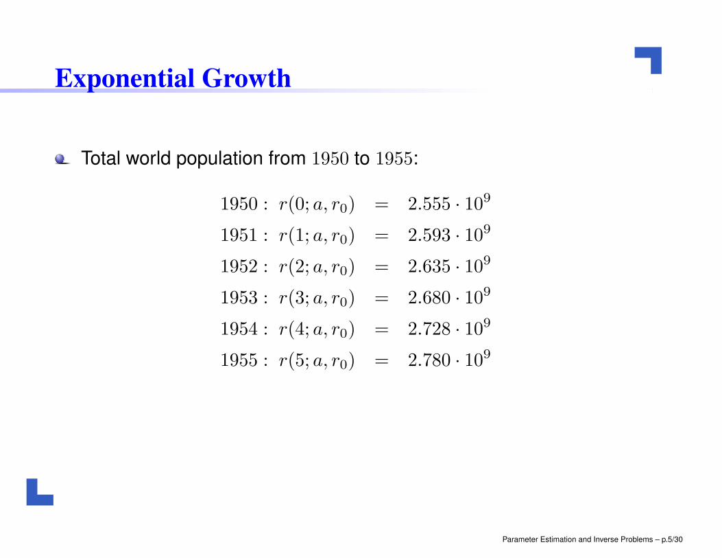
Total world population from 1950 to 1955:

1950 : r(0; a, r0) = 2.555 · 109

1951 : r(1; a, r0) = 2.593 · 109

1952 : r(2; a, r0) = 2.635 · 109

1953 : r(3; a, r0) = 2.680 · 109

1954 : r(4; a, r0) = 2.728 · 109

1955 : r(5; a, r0) = 2.780 · 109


Exponential Growth

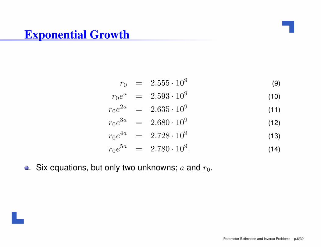
r0 = 2.555 · 109 (9)

r0ea = 2.593 · 109 (10)

r0e2a = 2.635 · 109 (11)

r0e3a = 2.680 · 109 (12)

r0e4a = 2.728 · 109 (13)

r0e5a = 2.780 · 109. (14)

Six equations, but only two unknowns; a and r0.


Cost-functional

Consider the function

J(a, r0) =1

2

t=5∑

t=0

(r(t; a, r0)− dt)2

=1

2

t=5∑

t=0

(r0eat

− dt)2,

where

d0 = 2.555 · 109, d1 = 2.593 · 109,

d2 = 2.635 · 109, d3 = 2.680 · 109,

d4 = 2.728 · 109, d5 = 2.780 · 109.


Cost-functional

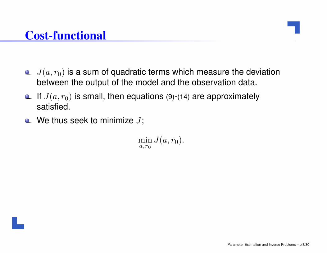
J(a, r0) is a sum of quadratic terms which measure the deviation

between the output of the model and the observation data.

If J(a, r0) is small, then equations (9)-(14) are approximately

satisfied.

We thus seek to minimize J ;

mina,r0

J(a, r0).


Cost-functional

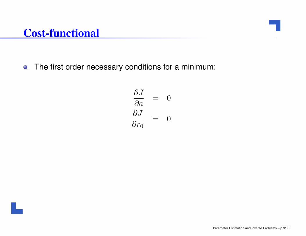
The first order necessary conditions for a minimum:

∂J

∂a= 0

∂J

∂r0= 0


Cost-functional

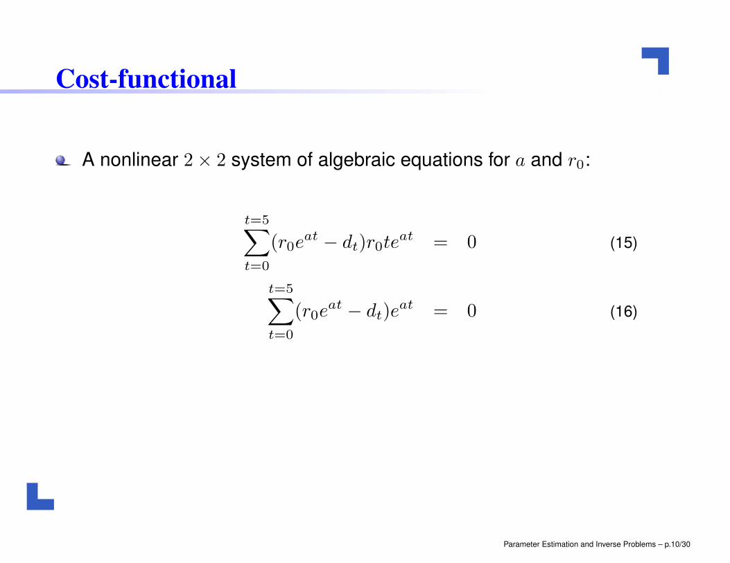
A nonlinear 2× 2 system of algebraic equations for a and r0:

t=5∑

t=0

(r0eat

− dt)r0teat = 0 (15)

t=5∑

t=0

(r0eat

− dt)eat = 0 (16)


Cost-functional

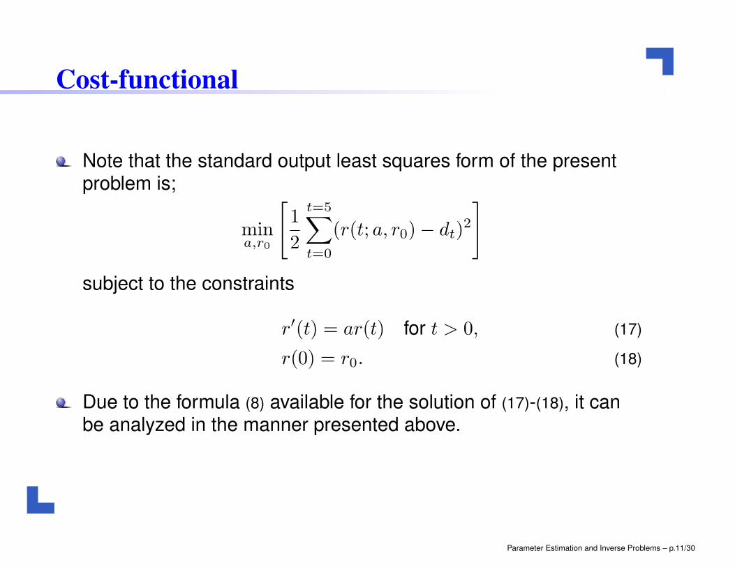
Note that the standard output least squares form of the presentproblem is;

mina,r0

[1

2

t=5∑

t=0

(r(t; a, r0)− dt)2

]

subject to the constraints

r′(t) = ar(t) for t > 0, (17)

r(0) = r0. (18)

Due to the formula (8) available for the solution of (17)-(18), it canbe analyzed in the manner presented above.


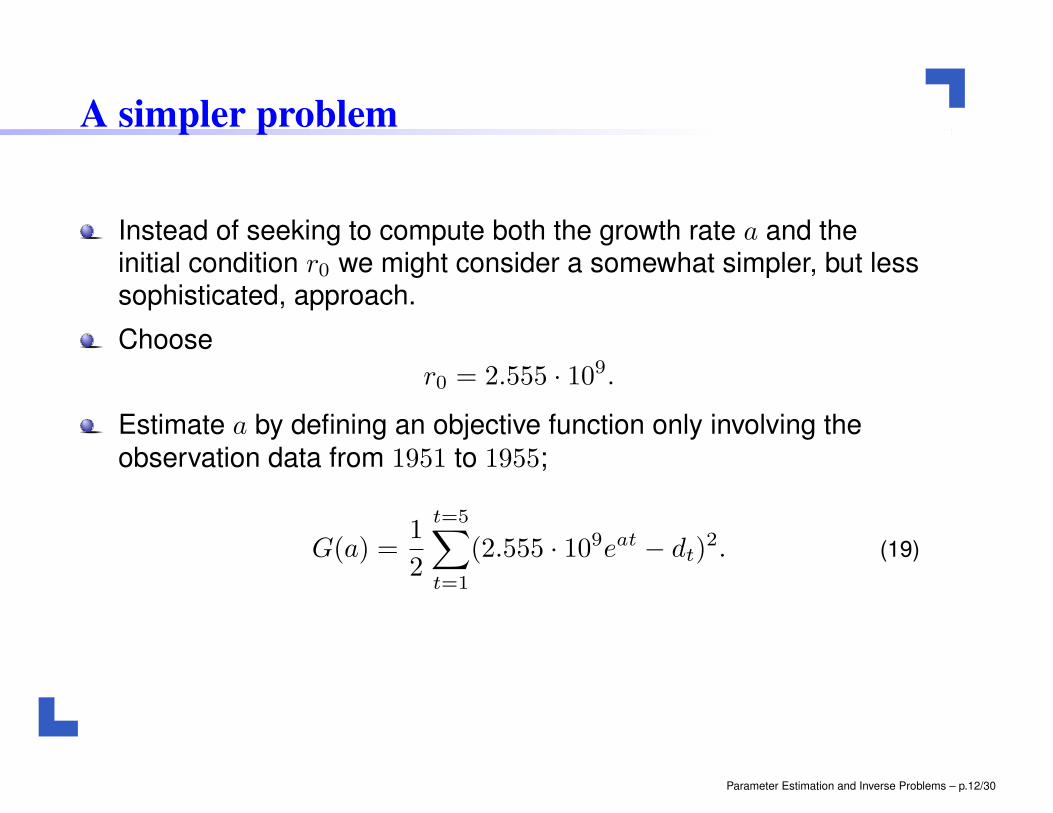
A simpler problem

Instead of seeking to compute both the growth rate a and theinitial condition r0 we might consider a somewhat simpler, but lesssophisticated, approach.

Choose

r0 = 2.555 · 109.

Estimate a by defining an objective function only involving the

observation data from 1951 to 1955;

G(a) =1

2

t=5∑

t=1

(2.555 · 109eat − dt)2. (19)


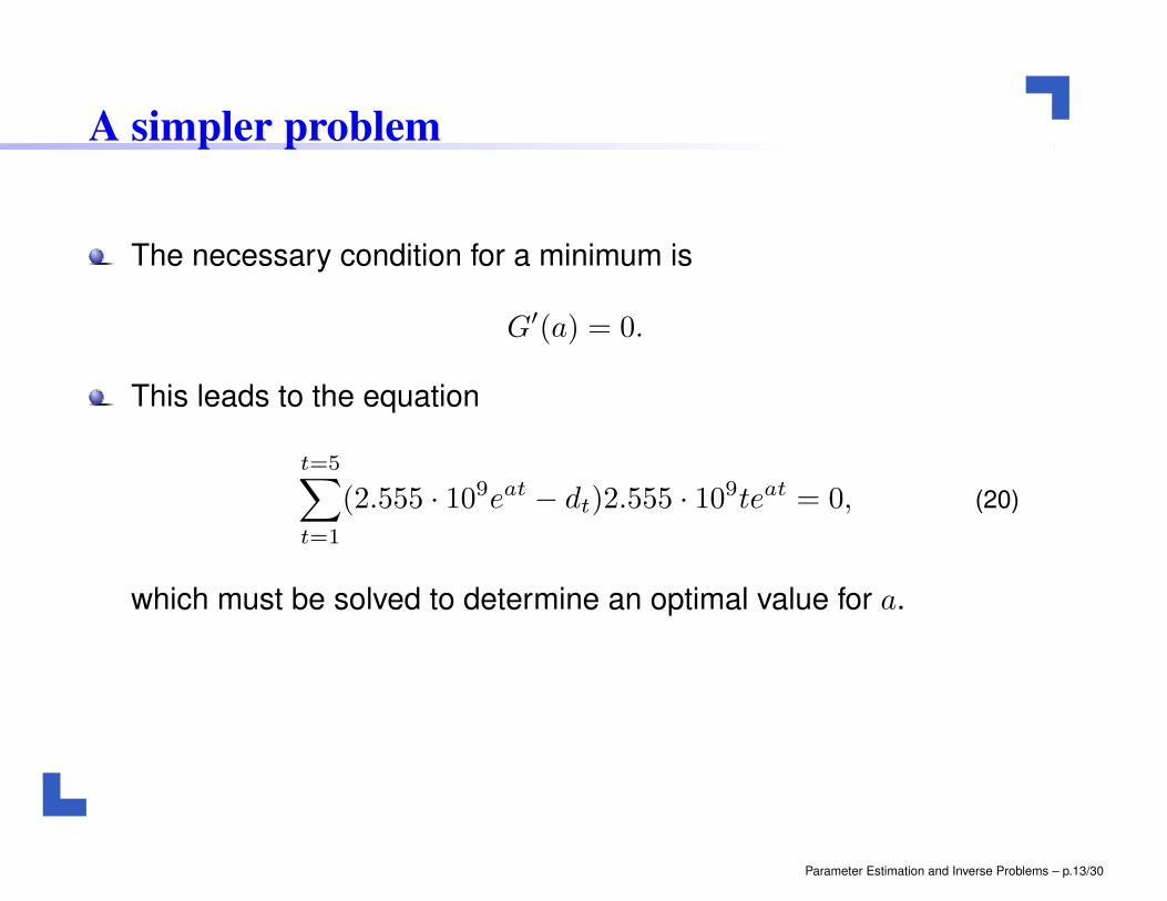
A simpler problem

The necessary condition for a minimum is

G′(a) = 0.

This leads to the equation

t=5∑

t=1

(2.555 · 109eat − dt)2.555 · 109teat = 0, (20)

which must be solved to determine an optimal value for a.


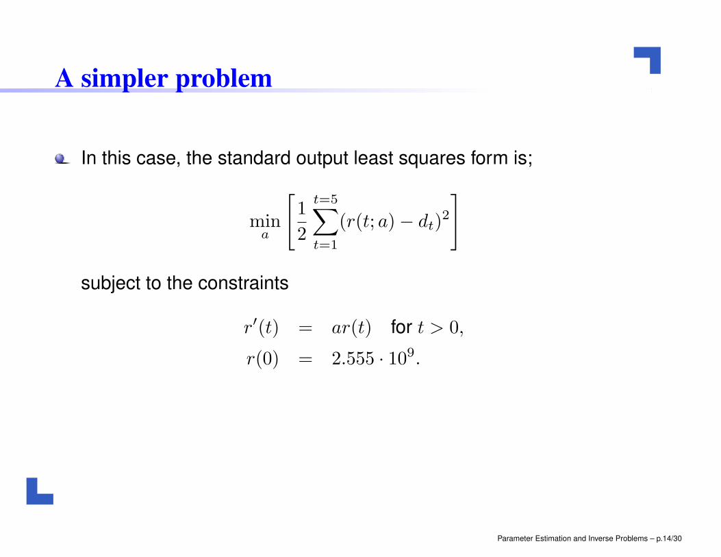
A simpler problem

In this case, the standard output least squares form is;

mina

[1

2

t=5∑

t=1

(r(t; a)− dt)2

]

subject to the constraints

r′(t) = ar(t) for t > 0,

r(0) = 2.555 · 109.


Backwards heat equation

Assume that a substance in an industrial process must have a

prescribed temperature distribution, say g(x), at time T in the

future.

The substance must be introduced/implanted to the process attime t = 0. (This could typically be the case in various molding

process or in steel casting).

What should the temperature distribution f(x) at time t = 0 be in

order to assure that the temperature is g(x) at time T?



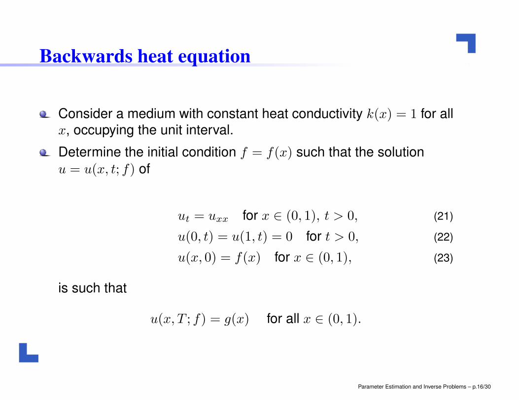
Consider a medium with constant heat conductivity k(x) = 1 for all

x, occupying the unit interval.

Determine the initial condition f = f(x) such that the solution

u = u(x, t; f) of

ut = uxx for x ∈ (0, 1), t > 0, (21)

u(0, t) = u(1, t) = 0 for t > 0, (22)

u(x, 0) = f(x) for x ∈ (0, 1), (23)

is such that

u(x, T ; f) = g(x) for all x ∈ (0, 1).



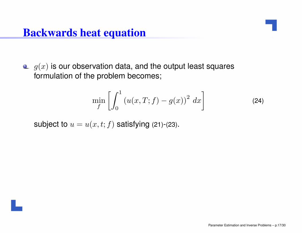
g(x) is our observation data, and the output least squares

formulation of the problem becomes;

minf

[∫1

0

(u(x, T ; f)− g(x))2dx

](24)

subject to u = u(x, t; f) satisfying (21)-(23).


Fourier Analysis

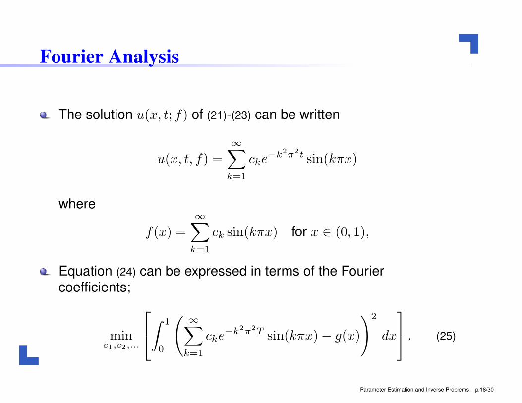
The solution u(x, t; f) of (21)-(23) can be written

u(x, t, f) =

∞∑

k=1

cke−k2π2t sin(kπx)

where

f(x) =∞∑

k=1

ck sin(kπx) for x ∈ (0, 1),

Equation (24) can be expressed in terms of the Fouriercoefficients;

minc1,c2,...

∫

1

0

(∞∑

k=1

cke−k2π2T sin(kπx)− g(x)

)2

dx

. (25)


Fourier Analysis

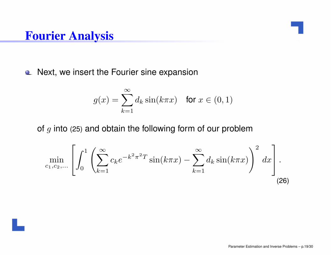
Next, we insert the Fourier sine expansion

g(x) =

∞∑

k=1

dk sin(kπx) for x ∈ (0, 1)

of g into (25) and obtain the following form of our problem

minc1,c2,...

∫

1

0

(∞∑

k=1

cke−k2π2T sin(kπx)−

∞∑

k=1

dk sin(kπx)

)2

dx

.

(26)


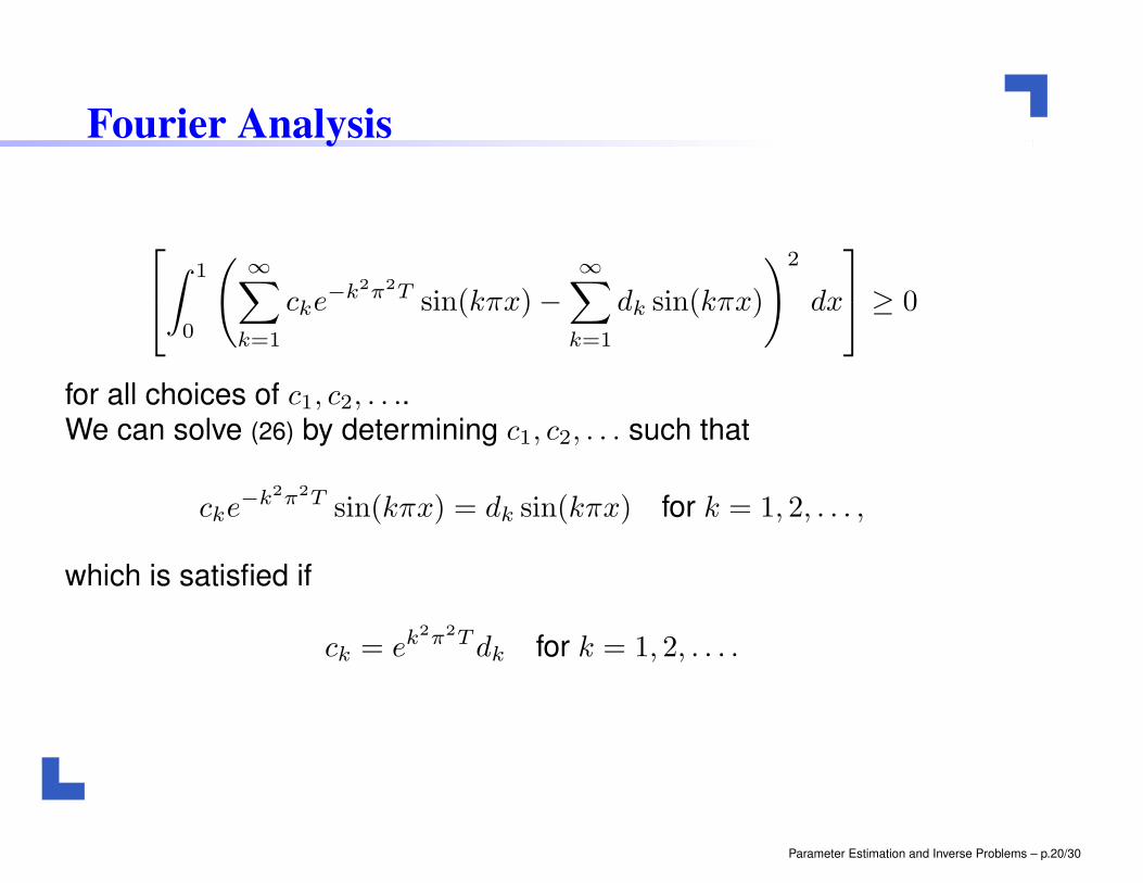
Fourier Analysis

∫

1

0

(∞∑

k=1

cke−k2π2T sin(kπx)−

∞∑

k=1

dk sin(kπx)

)2

dx

≥ 0

for all choices of c1, c2, . . ..We can solve (26) by determining c1, c2, . . . such that

cke−k2π2T sin(kπx) = dk sin(kπx) for k = 1, 2, . . . ,

which is satisfied if

ck = ek2π2T dk for k = 1, 2, . . . .


Fourier Analysis

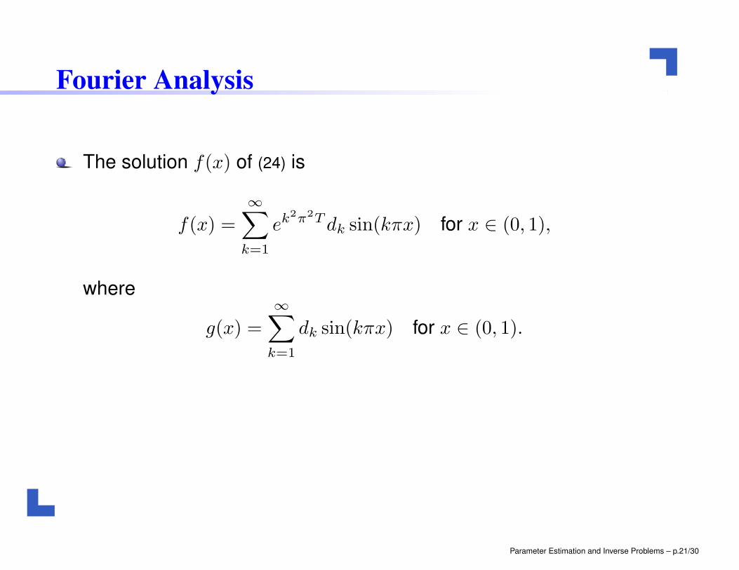
The solution f(x) of (24) is

f(x) =

∞∑

k=1

ek2π2T dk sin(kπx) for x ∈ (0, 1),

where

g(x) =∞∑

k=1

dk sin(kπx) for x ∈ (0, 1).


Stability

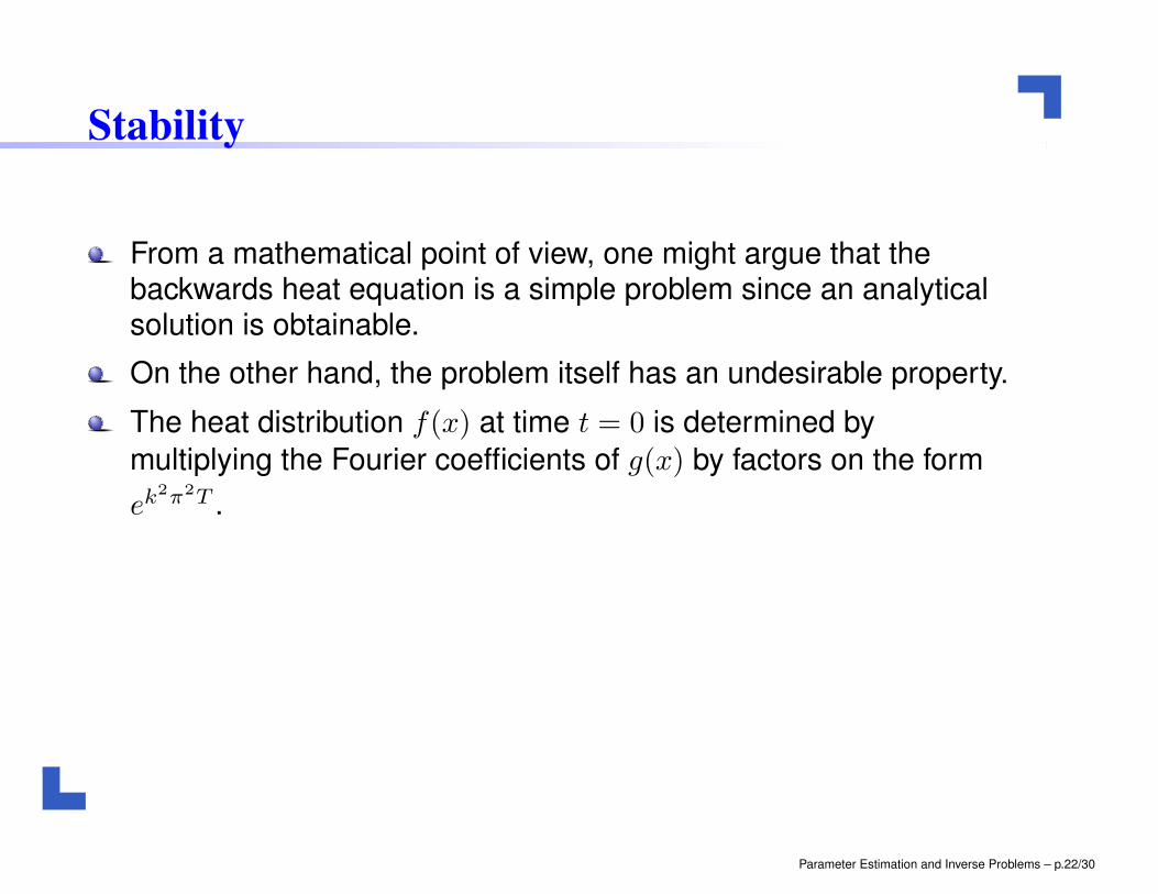
From a mathematical point of view, one might argue that thebackwards heat equation is a simple problem since an analyticalsolution is obtainable.

On the other hand, the problem itself has an undesirable property.

The heat distribution f(x) at time t = 0 is determined by

multiplying the Fourier coefficients of g(x) by factors on the form

ek2π2T .


Stability

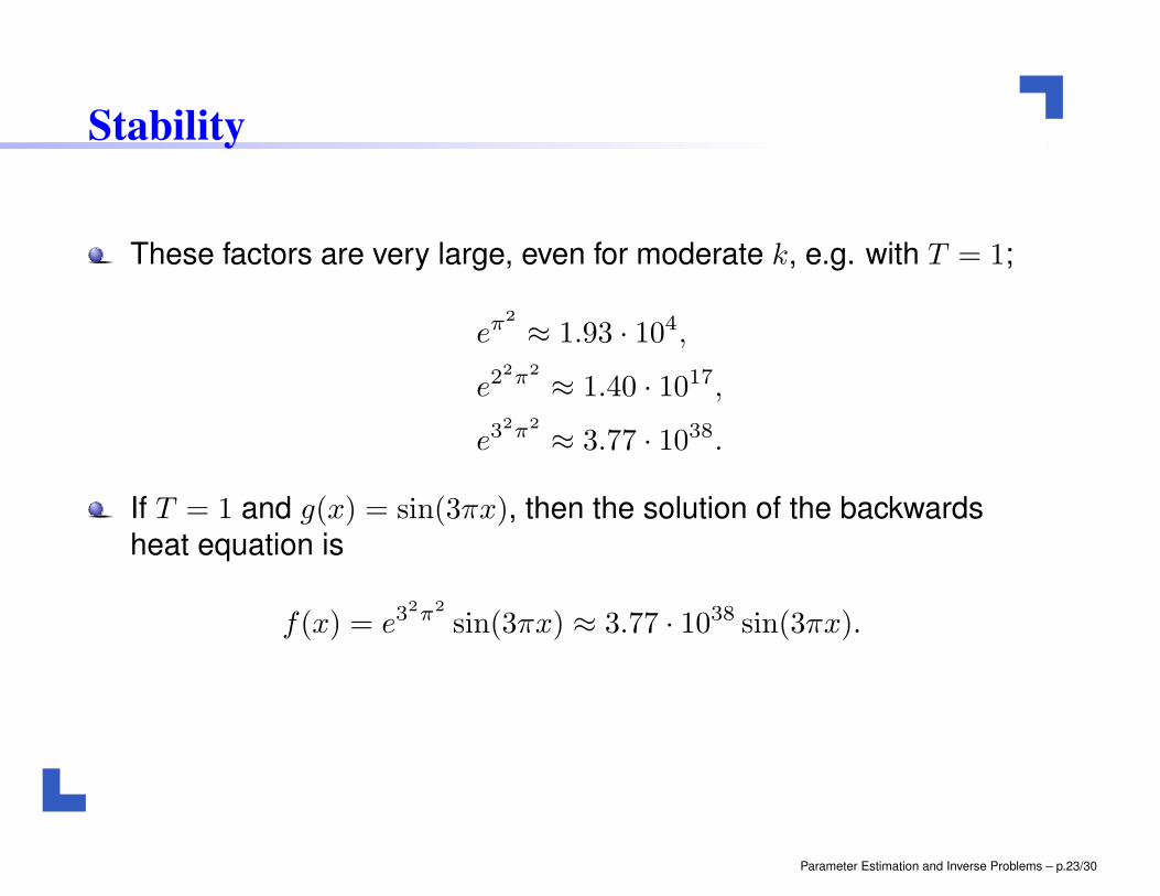
These factors are very large, even for moderate k, e.g. with T = 1;

eπ2

≈ 1.93 · 104,

e22π2

≈ 1.40 · 1017,

e32π2

≈ 3.77 · 1038.

If T = 1 and g(x) = sin(3πx), then the solution of the backwards

heat equation is

f(x) = e32π2

sin(3πx) ≈ 3.77 · 1038 sin(3πx).


Stability

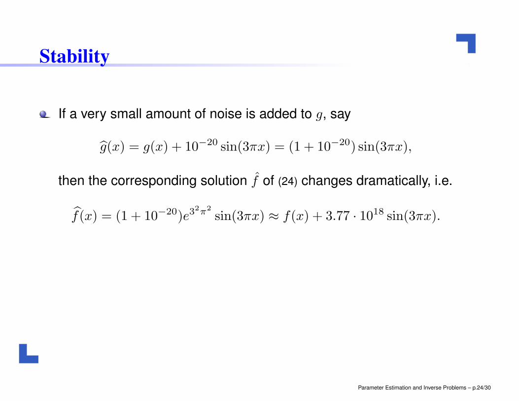
If a very small amount of noise is added to g, say

g(x) = g(x) + 10−20 sin(3πx) = (1 + 10−20) sin(3πx),

then the corresponding solution f of (24) changes dramatically, i.e.

f(x) = (1 + 10−20)e32π2

sin(3πx) ≈ f(x) + 3.77 · 1018 sin(3πx).


Stability

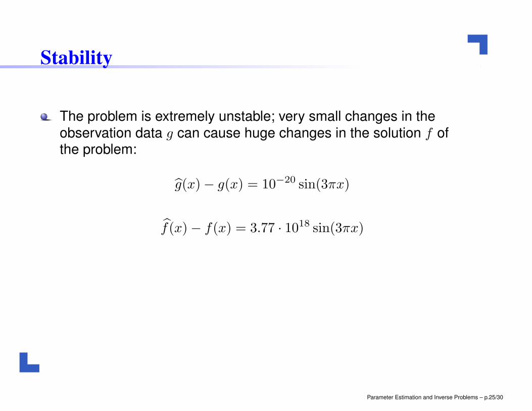
The problem is extremely unstable; very small changes in the

observation data g can cause huge changes in the solution f ofthe problem:

g(x)− g(x) = 10−20 sin(3πx)

f(x)− f(x) = 3.77 · 1018 sin(3πx)


Stability

One can argue that it is almost impossible to estimate thetemperature distribution backwards in time, only using the presenttemperature and the heat equation.

Further information is needed.

This has lead mathematicians to develop various techniques for

incorporating a priori data, for example that f(x) should be almostconstant.

More precisely, a number of methods for approximating unstableproblems with stable equations have been proposed, commonlyreferred to as regularization techniques.


Stability

Do the mathematical considerations presented above agree with

our practical experiences with heat conduction?

Is it possible to track the temperature distribution backwards intime in the room you are sitting?

What kind of information do you need to do so?


Estimating the heat conductivity

The examples discussed above are rather simple since explicitformulas for the solutions of the involved differential equations areknown.

This is not always the case, and we will now briefly consider sucha problem.

Assume that one wants to use surface measurements of thetemperature to compute a possibly non-constant heat conductivity

k = k(x) inside a medium.



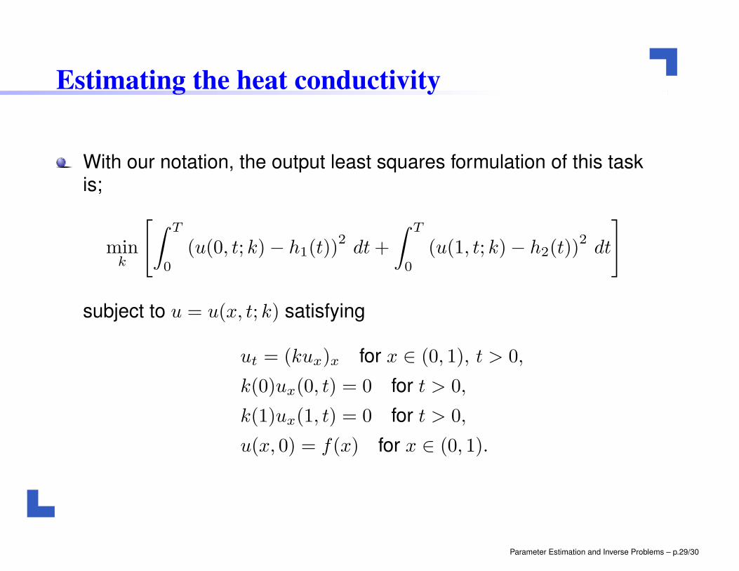
With our notation, the output least squares formulation of this taskis;

mink

[∫ T

0

(u(0, t; k)− h1(t))2dt+

∫ T

0

(u(1, t; k)− h2(t))2dt

]

subject to u = u(x, t; k) satisfying

ut = (kux)x for x ∈ (0, 1), t > 0,

k(0)ux(0, t) = 0 for t > 0,

k(1)ux(1, t) = 0 for t > 0,

u(x, 0) = f(x) for x ∈ (0, 1).



This is a very difficult problem.

To solve it, a number of mathematical and computationaltechniques developed throughout the last decades must beemployed.

This exceeds the ambitions of the present text, but we encourage

the reader to carefully evaluate their understanding of the output

least squares method by formulating such an approach for a

problem involving, e.g., a system of ordinary differential equations.


Documents

Parameter Estimation and Inverse Problems