Parameter Estimation for 3-D Ceoelectromagnetic Inverse Problems

Ol eg Portniaguine

M ich ael S. Zhdanov

Summary. Param eter estimation in geoelectromagnetics aims to obtain the most im ­portant param eters of a well-defi ned conductivity model of the Earth. These param eter s

are features of typi cal geo log ica l struc tures, such as depth and size of con duct ive or

resistive targets, angle of dik e incl inat ion and its length, and con duct ivity of anoma lous bodies. We dev elop thi s approach through regul arized nonlinear optimization. We use

finite differenc es of forward co mp utations and Broydens updatin g formula to compute sensitivities (Frechet or partial der ivatives ) for each parameter. To estimate the op tim al

step length , we appl y line sea rch, with a simple and fast parab olic correction . Our in­version also includes Tikhonov's regul ariz at ion proced ure. We use our meth od to study

mea surement s of the magnet ic fields fro m a co nductive bod y exc ited by a loop source at

the surface. Keeping the depth of the bod y co nstant. we estima te the hor izont al coordi­nates of the body from three comp one nts of the magnetic field measured in a borehole. Th ese measurem ent s acc ura tely determine the directi on to the conductive target.

1 Introduction

In the past decade, man y ad vances have occ urred in multidimension al inversion of

dc resistivity data (Shima, 1992; Oldenburg and L i. 1993 ; Sasaki, 1994; Zh ang et al., 1994) , and both tran sient and harm oni c electromag netic (E M) data (Eato n, 1989;

Madden and Mack ie, 19R9; Smith and Booke r, 1991 ; Xiong and Kirsch, 1992: Lee and Xie, 1993 ; Pellerin er al ., 1993; Tripp and Hohmann, 1993; Nekut, 1994 ; Torres ­Verdin and Hab ashy , 1994; and Zhdanov and Fang, 1995) . Mo st of the advances came in

inversion for models with many ce lls of constant conductivity, in whi ch an opt imizat ion

algorithm finds a distribution of co nductivity whose response matches the original data . These methods all face the difficulties of large- sca le inversion: Computer power and

mem ory ca pac ity grow ex ponentially with the number of cells, and the stability of the inverse problem gets wo rse (Tikho nov and Arse nin, 1977 ).

When interpretin g EM data, however, one often ca n construct seve ral possible geo ­

e lectrical model s on the basis of prior geo logica l and geophysical informatio n. All o f

Univers ity of Utah, Dep artment of Geology and Geoph ysics. Salt Lake C ity, UT 84 112.

222

Parameter estimation for inverse problems 223

these models co uld co ntain the same geologi cal structure, but with di fferent spec ific parameters- say, depth and size of conduct ive or resis tive targets, ang le of dike incli­nation and its length , and conductivity of the anomalous bodies . The goa l of inversion then becomes the es timation of a few important param eters of the model. Inversion for only a few parameters is, of cour se , more efficient than a genera l inversion. The first EM inversions (in the 1970s) were paramet ric ; however, they were lim ited to one­dimensiona l ( ID) layer thicknesses and con ductivities. We take up this approac h, but with all of the adva ntages of modern 3-D forwa rd model ing.

2 Inversion scheme

2.1 Minimization problem

A ge nera l approach to ill-pose d inverse problems is based on minimization of the Tikhonov parametric func tio na l (Tikhonov and Arsenin, 1977),

rem) = ¢(m) + as( m) = min. ( I )

where ¢ is a misfit functional,

¢( m) = lI r(m )II ~ , r em) = A( m) - d"; (2)

d" is the vec tor of N observed EM da ta; m is the vector of M model parameters; Atm) is the vector of theo retical (predicted) EM da ta; r em) is the residu al vector; and sCm)

is the stabilizing functiona l

sCm) = 11 m- map, l( (3)

Minimi zing Eq. ( I) replaces the orig ina l ill-posed inverse probl em with the family of we ll-pose d problem s, which tend to the orig inal problem as the reg ularization param eter a goes to zero (Tik honov and Arsenin, 1977). Eve ntua lly. we want to find the model that bes t fits the obse rved data . The stabi lizing func tiona l (3) is designed to kee p the inverse model relatively close to so me prior reference mode l map,. The min imization prob lem ( I) is solved for different values of the regul arization para mete r a . We ca n select the qu asi-optimal value of a by usin g prior inform at ion abo ut the acc uracy of the orig ina l data.

2.2 Optimization method

Our inve rs ion code has optio ns for using conj uga te gradient, steepest descent, and New tonian methods. We usually use only a few free parameters, so that the Hessian matrix has a sma ll size . This allows us to use New ton's method which has a superior conversio n rate.

The method iteratively updates the model at the i th iteration according to formul as

mi+1 = mi + omi. (4)

om;= kom;, (5)

om;= - [IJ(mil + aIr ' f "'(m ;), (6)

fU(m,) = r(mj) r trn .) + a(m ; - m ap,) , (7)

t!(rn ;) = r(m ;) f (rn j) , (8)

224 Portniaguine and Zhdanov

where 8m; is the Newtonian step, om; is the corrected Newtonian step, k is the correction factor, f " (m. ) is the regularized direction of the steepest ascent, fCm;) is the Frechet derivative matrix of size N x M, Ij(mi) is the Hessian matrix of size N x M, and! is the unit matrix. An asterisk denotes the conjugate transposed matrix.

The length of the Newtonian step 8m; is determined by assuming that the parameteric functional is a perfect quadratic which is only true for a linear inverse problem . To improve convergence for nonlinear functionals, the step length should be chosen by a search for a minimum along the direction of the Newtonian step (Fletcher, 1981):

P" ( k8 ' ) - . ,m; + m; - mm .. (9)

We apply the simplest one-step search that assumes parabolic behavior of the residuals run.) at point rn.:

r(m; + kom;) = ek' + g(m;)k + r(rn.).

The ease k = I corresponds to the classical Newtonian step without correction, We compute the residual rem; + 8m;) at the destination point of the Newtonian step: then, knowing the gradient along the step direction glm i) =Fun,)8m; and the residual rtm.) at the current point , we can estimate the vector c which consists of the second derivative of the residuals:

c = r(m; + 8m;) - gem;) - r tm .). (l0)

Equation (9) thus can be replaced by the fourth-ord er polynomial with respect to k. , if we know the residual r( rn, + 8m;) at the destination point of the Newtonian step:

IIck2 + g(m ;)k + r em;) 11 2 + a 11m; - mapr + k8m; r= min l. (II )

The norm of any vector B is IIBI12 = WB. We can rewrite Eq. (II ) in the form of the scalar fourth-order polynomial minimization problem with respect to parameter k as

Po + p-]: + P2k:' + P3k3 + V.e = mini , ( 12)

where polynom ial coefficients are defined as

Po = Ilr (mi)112 + a ll m; - mapr ll:',

PI = 2 Re[g (m;)*r(m;) + a (m; - mapr)' 8m;] ,

P2 = Ilg(m; )11:' + a 118m; r + 2 Rejc tr(m, )],

p, = 2 Re[c*g(m; )1, P. = c*c.

We solve Eq. ( 12) numerically using the secant root-finding method and select the smallest positive root as an optimal step length , because we have to be conservat ive and stay close to the previous iteration.

2.3 Frechet derivatives

The elements F (k l) of the Frechct (partial) derivative matrix, which are required in formulas (7) and (8) to comput e the Newtonian step, can be estimated with finite

225 Parameter estimation for inverse problems

differences:

3d(k) A lk )[m + omIt )] - Alkl(m) F lkf) = -- ~ , ( 13)

dm(f) om(f)

where d (k) is the kth element of the vector of data and omIt ) is a small perturbation

of the lth element of the vector of parameters. In numerical calculations we select a perturbation equal to I% of corresponding parameter value. To 1111 out the whol e matrix, we have to apply formula (13) for each parameter.

To save computational time , the Frechet matrix on the next step, f i+l, can be esti­mated from the Frechet matrix on the previous step, fj, using the approximate Broyden updating formula (Fletcher, 1981; Gill et al., 1981). To derive the Broyden formula,

we express the Frechet derivative f i+1 at the point mi+1 as a difference between the forward solution A(mi+l) at the subsequent iteration mi+1 = m, + omj and the forward soluti on for the current iteration A(ID;):

f i+l om j ::::::: A (m j-rl) - A(mi)' (14 )

However, knowing the current Frechet derivative f i. we also can express its variation

t>f, as

t>fi ;:; f i+l - Vi. (15 )

Let F (k l stand for the kth row of the Frechet derivative matrix. Then, combining Eqs. ( 14) and (15 ) g ives the underdetermined system of N equations with respect to N x M elements of the matrix t>f;:

AF1k-) O , _ S lk ) L\ _ i om, - i • k=1.2 .... N . ( 16)

where

S i k) = A 1kl(m ;+ I ) - A 1kJ(1I1 i ) - F? )omj . (17)

Thi s system of equations ha s a unique so lution under the additi onal condition that the vectors t>F;kl have the minimum norm,

IIt>Fjk)II = min . (18)

According to the Riesz representation theorem (Parker, (994), the so lution of Eqs. (16 ) under condition (18) can be written as

lk -) (k) Tt>F i = J,. om; , k=I,2. 3, .. . ,N, (19)

where lk )are unknown constants determined from the equation

j .(k)omT 8m" = S lk ) (20)1 I l •

and om; is a row vector of the parameter perturbation (transpose-or-column vector omi)' So lving Eq . (20) and substituting the result into Eq. ( 19) give s

S(k l o T , u rn ,t>Flk- -I = ! , ' . (21)

! om; 8m;

Using formula ( 15) for the Frechet deri vative Vi+1 and expression ( 17) gives the first­order Broyden updating formul a

' F - om;F = ~i+ rA(mj+ I) - A(mi) - fi8mi ] . T' (22)_ '+I (~ mi 8m;

i

Portniaguine and Zhdanov 226

At the starting point of the iteration proces s, we apply formula (13) to estimate the Frechet matrix, take a Newtonian step using formula (6), solve the forward problem at this point, and estimate a correction factor k, solving Eq. (11) . Then, we take the corrected step, using formula (5) . At the arrival point, we estimate a new Frech et derivative, using Eq, (22), and take a new Newtonian step. If the correction fails to make progre ss (the parametric functional increases), the Frechet derivative is reevaluated using expression (13).

When the correction factor k is close to zero , we assume that we have reached the minimum of the problem, and we adjust the regularization parameter using the expression anew = Ciold /2, and continue with the new value of a. Global iterations stop after the misfit functional drops below the given accuracy level. An application of this method for the simple nonlinear inverse problem is shown in Fig. 1. The nonlinear problem to be solved is described by the following system of equations:

2 X

3 + i = 5, x - Y = -1 , - 2x + 2/ = 6.

We define the misfit funtional ¢ (x, y) as

3200 1 0 0¢ (X ,y)= (x +y -5t+ (x"- y +I )-+(-2x+2y--6)-.

The inversion path is shown by the dashed line in Fig . I. The solid line shows isolines of the misfit functional. It has a minimum at the solution point (x = 1, y = 2). Iteration starts from the point x = 0.4, y = I, which is marked by the asterisk in Fig. I . At this point the Frechet matrix is estimated using a finite-difference method. The iteration step

2~1- - '

~~~~ 2 f ' C2>~~G:>. I \ "< /

\

1.5

~

0.5 ' I I 1

0.5

II I

\ I

Il

o 1.5 2 2.5 1 x IFigure 1. Example of opt imization for nonlinear problem with two parameters. !

'., 1j

'~

.1 .

Parameter estimation for inverse problems 227

brings us to the point shown by the cross. Note that the step length is overe stimated. A parabolic correction reduces the step to the local minimum, shown by the circle. At this point the Frechet derivative is estimated using the Broyden formula, and the next step is performed in a new direction. Iterations converge rapidly to the global minimum.

The main advantages and disadvantages of the numerical computation of the sensi­I,

tivities are well known. The disadvantage is that, for a problem with Nm parameters, we have to solve the forward problem Nm + I times, whereas algorithms based on the

If

quasi-analytic solution for Frechet derivatives require computing efforts equivalent to two forward modeling runs for each estimation.I

". One advantage of our approach is the possibility of choosing nontrivial inversion

~ . parameters, e.g., depth and coordinates of the anomalous body and its resistivity, size of the conductive or resistive target, and angle of inclination. In the next section, we

...., demonstrate the effectiveness of our inversion scheme on a synthetic model.

.?

3 Directional sensitivities of three-component magnetic data

EM observations in a single borehole that can provide direction to the target are poten­tially intere sting both for mining and oil and gas applications. In mining exploration, it is important to give accurate direction to off-hole conductors. In oil and gas applica­tions , a system with directional sensitivity can be used for navigation of the bit during horizontal drilling. Today, there are numerous borehole tools built for the downhole measurement of three components of a magnetic field (Crone Geophysics & Exploration

t

:~ Ltd., 1995. Three component borehole survey: Flying Doctor Prospect, Broken Hill, Australia). Studying a model of a 3-D conductor, we demonstrate that three-component measurements have good directional sensitivity.

J Consider the model of a conductive body located at a depth of 150 rn, 80 m away".' from a borehole in the x-direction (Fig. 2). The transmitter is a circular loop 200 m >,r

~ in diameter with the center at the coordinate origin. Eleven receivers are located in .-:....

the borehole and are spaced equally within the depth range from 100 to 200 m. The" body is a cube with a side of 60 m. Conductivity of the body is I ohm-rn , whereas

f !l ' background conductivity is 1000 ohm-m. The theoretical time-domain magnetic field ~~

:'. in this model was simulated within the time range from I flS to 1000 us using TEM3-DL finite-difference code (Wang and Hohmann, 1993).

The data are three components of the magnetic field measured along the single .. observation line (borehole). It is obvious that the depth of the body can be determined~

by the location of the maximum of the secondary field in the vertical profile . However, ( ,­ our goal is more complicated. We would like to determine the distance and the direction p.i : from the borehole to the conducting body.

,1­j:,.' Thus, we can fix the depth ofthe body and introduce the polar coordinates of the body

> center: the distance R from borehole to the body and the angle (J between the x-axis and ... .., the direction to the body center (Fig. 2). The actual polar coordinates of the conductive

c' body are R = 80 m and (J = O. The synthetic data for this model (IJ H?/IJt for all 0'

'-~ '. receivers, with 5% random noise added) are shown in Fig . 3. The inverse problem is reduced in this case to determining (R, fJ) for given EM data.

We introduce the misfit functional s <Pr, <Py , <P:, defined as the norm of the difference

. . between the corresponding x, y, or z components of the predicted aR/at and actual ~ ~

";,:

iI<

i· tor

,:.. ,

""

.v .r­ - .~ " . .• _, I,

150m

60m

/1!21/ p=1 L-L~ . Ohrn-rn ' I,T '/~ I /

lL-.-_v

z

: I i - 0 '! ~

;<::. :9- _. __ R

*cp

6 I ~

100m

II receivers

p=IOOO Ohm-rn

Figure 2 . Survey design and model used for direct ional sens itivity investigation.

100 -

500

200

- ---------­ .,' x, ' ~-' 0 7 _ ~_'_> V 21 -----<---8 __~~ , - -~--------­ . - - -~

Y /: I ;I : i

I100 m : !

<: - - - - - - - - - - - _ . _ -- - - - - - - - - - -_ . _ - - -_. _ - - - - -_ . _ - -- - ~

Portniaguine and Zhdanov

iooo 100 110 120 130 140 150 160 170 180 190 200

Depth (m )

Loop diameter 200 m

'" " '~

-=­.§ 50 '­

1-­ ! -+= ! -j ·t, -10.7 -5.9 -1.8 -0.1 -0.0 0 .0 0.1 0.2 0 .5 1.8

m Volt s

Figure 3 . T ime derivati ve of the magnetic field (x -co mponent) from the actual model (5% random noise added ).

228

"l

229 Parameter estimation for inverse problems

- 100

-so

4 0

- -20 ;....

§ v

;; --:;;"

20 c5

-10

60

-100 -80 ..fIJ 40 -20 0 20 -10 60 80 100 Distance on X ( Ill ')

~ .. _ ----~~

0.0000 O.oJ"5 0.0630 0.083 1 0.I IS5 l JXXXJ Norm alized misfit

Figure 4. Misfit functional for z-component versus horizontal coord inates of the body.

()H1l /iJrmag netic field:

<P , = IlaH,/iJ t - a H~/ ar l lz. <P, = IlaHv/at - a H~.) / arf

<P: = Il a H~ / at - oH2/arf and the misfit func tiona l <P r. is defined for all three components,

<Pr. = <P, + <p.' + <p~ .

where we use the Lz norm over the time interval of the magnetic-field observation .

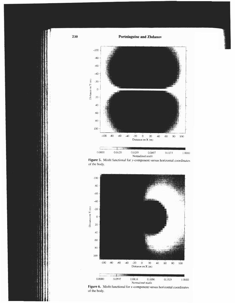
The plots of misfi t functionals <P: . <Py. <P" and <Pr. as functions of the horizont al coordinates of the bod y are presented in Figs. 4. 5. 6. and 7, res pectively. We expec t tha t the misfit functionals have minim a at the location of the body. However. the modeling results show that the z-cornponent is se nsitive only to the di stance to the body R. but is not sensitive to the direction e.The map of the misfit functional for this com ponent has a circ ular structure with the circul ar minimum correspo ndi ng to an 80- 01 radius (Fig . 4) . At the same time , the <Pv misfit functional corresponding to the y-corn ponent of the mag netic field has a minimum everywhere along the x -axis, but it gives no information about the distance to the body (Fig. 5). The map of the <P, misfi t funct ional is rather complicated ; however, it has a weak and flat minimum in the vicinity of the body location (Fig. 6). Onl y the combination of three components produ ces a clear minim um on the map of <P r. at the true locat ion of the body (Fig. 7) .

-100 -80 -60 --10 -20 0 20 40 60 80 100 Distance on X (m )

1.(X)()(J

1.0000

0 .1173

0.1525

Portniaguine and Zhdanov

t===E 0.0 120

0.0597

L o.ocoo

0.0000

- 100 1 I

-80 -'

i -60 -1

I

--10 ~ I I

- -10 I ;.. I

I

" 0 -1

J I ~ I 6 20 -1

40 1 (,() .1

I I so 1 I

100 "I "---­

·100 -80 -Ci) -40 -20 0 20 40 60 SO 100 Distance on X (rn)

so

--10

r

100

-60

80

_ -20 ;.. :: C 0 ~

~ ::S

0.0 255 0.0497 Normaliz ed misf it

Fi gure 5. Mi sfit functional for y-component versus horizon tal coordinate s of the body.

0.0816 0.1006 Normalized misfit

Figure 6. Misfit functional for x- component versus horizo ntal coo rdi nates of the bod y.

230

'r

L1

231 Parameter estimation for inverse problems

so

-GO

60

-80

100

- 100

'" -20 ;­

'" c 0" v

~ 20:5

-100 -80 ..6J --10 -20 0 20 -lO 60 SO 100 Dis tance on X ( Ill)

' _ l._~ _ • •:-=-_ _ __L_-,-,~Jj!lii.II• • • • • • 0.0000 0.0583 0 .07·+] 0.0813 0.0857 0 .0876 0 .09 11 0. 15 11 0 .3104 I.rxJOO

Normalized misf it

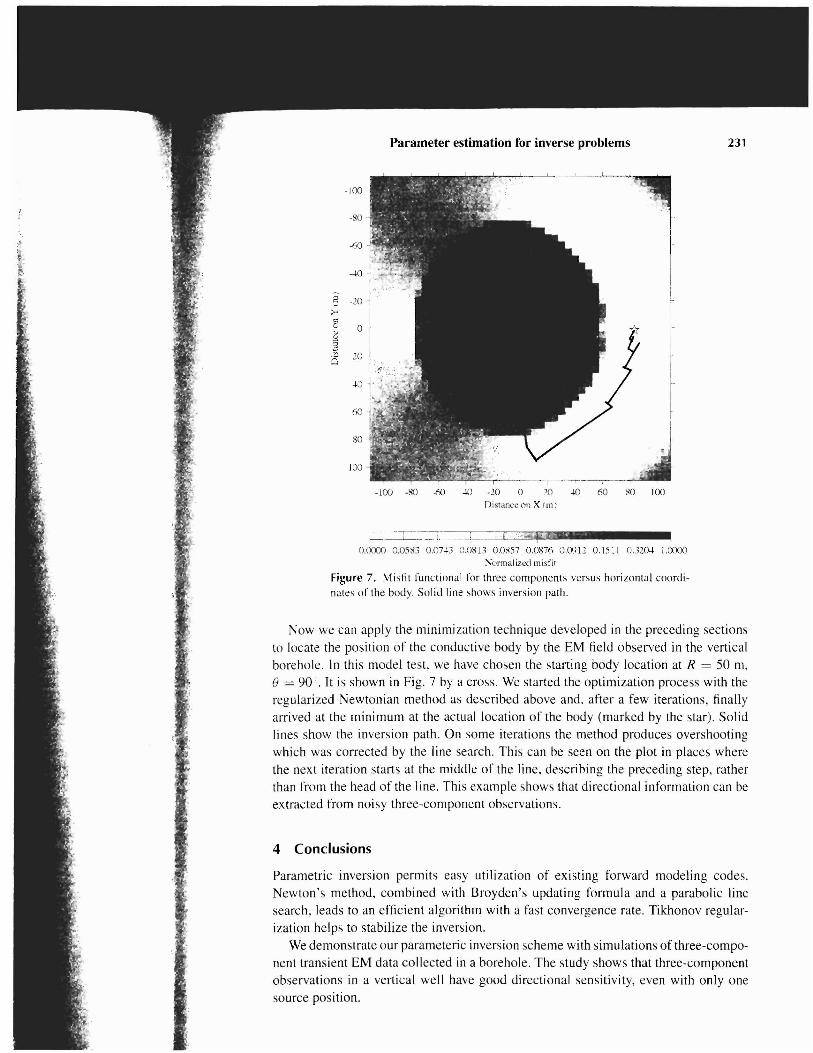
Figure 7. Mi sfi t functiona l fo r thr ee co mponent s versus hori zonta l coordi­

nates o f the body. So lid line shows inversion pat h.

Now we can apply the minimization technique developed in the preceding sections to locate the position of the conductive hody by the EM field observed in the vertical borehole. In this model test, we have chosen the starting body location at R = SO m, e = 90 ;. It is shown in Fig. 7 by a cross. We started the optimization process with the regularized Newtonian method as described above and, after a few iterations, fi nally arrived at the minimum at the actual location of the body (marked by the star). Solid lines show the inversion path. On some iterations the method produces overshooting which was corrected by the line search. This can he seen on the plot in places where the next iteration starts at the middle of the line, descrihing the preceding step, rather than from the head of the Iine. This example shows that directional information can be extracted from noisy three-component observations.

4 Conclu sions

Parametric inversion permits easy utilization of existing forward modeling codes. Newton's method, combined with Broydcn's updating formula and a parabolic line search, leads to an efficient algorithm with a fast convergence rate. Tikhonov regular­ization helps to stabilize the inversion.

We demonstrate our pararneteric inversion scheme with simulations of three-compo­nent transient EM data co llected in a borehole. The study shows that three-component observations in a vertica l well have good directional sensitivity, even with only one source position.

232 Portniaguine and Zhdanov

Acknowledgments

We thank the Consortium on Electromagnetic Modeling and Inversion at the Department of Geology and Geophysics, University of Utah , including CRA Exploration Ltd., Newmont Exploration, Western Mining, Kennecott Exploration, Schlumberger-Doll Research, Shell Exploratie en Produktie Laboratoriurn, Western Atlas, US Geological Survey, Zonge Engineering, MIM Exploration, BHP Exploration, and Mindeco for providing additional support for this work.

References

Eaton, P., 1989, 3-D electromagnetic inversion using integral equations: Geophys.

Prosp., 37, 407-426. Fletcher, R., 1981, Prac tical methods of optimization: John Wiley & Sons, Inc . Gill, P.. Murray, w.,and Wright, M., 1981, Practic al optimization: Academic Press Inc. Lee, K., and Xie, G., 1993, A new approach to imaging with low frequency electro­

magnetic fields : Geophysics , 58, 780-796. Madden, T R., and Mackie, R. L., 1989, Three-dimens ional magnetotelluric modeling

and inversion: Proc . IEEE, 77 , No.2, 318-332. Nekut, A., 1994, Electromagnetic ray-trace tomography: Geophysics , 59, 371-377. Oldenburg, D., and Li, Y, 1993, Inversion of induced pola rization data: Soc. Expl.

Geophys., Exp anded Abstracts, 396-399. Parker, R., 1994, Geophysical inverse theory : Princeton Univ. Press. Pellerin, L., Johnston, 1., and Hohmann, G., 1993, Three-dimensional inversion of

electromagnetic data : Soc . Expl. Geophys., Expanded Abstracts, 360-363 . Sasaki, Y, 1994, 3-D resistivity inversion using the finite-element method: Geophysics,

59, 1839-1848. Shima, H., 1992, 2-D and 3-D resistivity image reconstruction using crosshole data :

Geophysics, 57, 1270-1281. Smith, 1. T , and Booker, 1. Roo 1991, Rapid inversion of two- and three-dimensional

magnetotelluric data : J . Geophys. Res., 96, 3905-3922. Tikhonov, A. N. , and Arsenin, V. Y, 1977, Solution of ill-poised problems: W. H.

Winston and Sons. Torres- Verdin, C; and Habashy, T., 1994, Rapid 2.5-dimensional forward model­

ing and invers ion via a new nonlinear scattering approximation: Radio Sci., 29, 1051-1079.

Tripp, A. C; and Hohmann, G . W., 1993, Three-dimensional electromagnetic cross­well inversion: IEEE Trans. Geosci. Remote Sensing, 31, 121-126.

Wang, T, and Hohmann, G. W., 1993, A finite-difference time domain solution for three-dimensional electromagnetic modeling: Geophysics, 58, 797-809.

Xiong, Z., and Kirsch, A., 1992, Three-dimensional Earth conductivity inversion: J. Com put. App\. Math ., 42, 109-121.

Zhang, 1., Ma ckie, R., and Madden, T, 1994, 3-D resistivity forward modeling and inversion using conjugate gradients: Soc. Expl. Geophys ., Expanded Abstracts,

377-380. Zhdanov, M. S., and Fang, S., 1995, Quasi linear approximation in 3-D electromagnetic

modeling: Geophysics , 61 , 646-665 .