Parallel optimization applied to magnetoencephalography

Journal of Computational and Applied Mathematics 183 (2005) 177–190

www.elsevier.com/locate/cam

Parallel optimization applied to magnetoencephalographyTakashi Suzuki∗

Graduate School of Engineering Science, Osaka University, 1-3 Machikaneyama, Toyonaka, Osaka 560-8531, Japan

Received 8 September 2004; received in revised form 21 January 2005

Abstract

This paper studies a new numerical scheme applicable to magnetoencephalography (MEG), that is, clustering.This method is based on a new theory to the under-determined ill-posed problem, called parallel optimization,and clusters several electric current elements distributed in a volume conductor by one point in time data, withoutprescribing the number of dipoles. Numerical experiments and optional algorithms are also included.© 2005 Elsevier B.V. All rights reserved.

MSC:92C55; 65Y99; 49M05

Keywords:Magnetoencephalography; Inverse problem; Ill-posed problem; Parallel optimization; Clustering

1. Introduction

The purpose of the present paper is to propose the algorithm “clustering”, based on a new theory tothe under-determined variational problem, called parallel optimization, and is to examine its validity inmagnetoencephalography (MEG).In describing MEG, we note that the neuronal activity evokes the primary electric currentJp within the

brain, and it creates the magetic fieldB outside head. ThisB is around 10−8 of the geomagnetism, but weobtain noninvasive measurements using superconducting quantum interference device (SQUID), whichpossesses 100–300 channels on the interface between the head and the SQUID. In MEG, conversely, oneascertainsJp from such real time data ofB.

∗ Tel.:/fax: +81668506475.E-mail address:[email protected].

0377-0427/$ - see front matter © 2005 Elsevier B.V. All rights reserved.doi:10.1016/j.cam.2005.01.011

http://www.elsevier.com/locate/cam

mailto:[email protected]

178 T. Suzuki / Journal of Computational and Applied Mathematics 183 (2005) 177–190

To be more precise, from the quasi-static approximation[5], theseJp andB are governed by theGeselowitz equation[2,3], and if the shape of the brain is approximated to be spherical, then this equationis reduced to a simpler form[4] due to the simplification of the volume current term−�∇V , which arisesin accordancewith the electric field caused due toJp. If the dipole hypothesis is adopted, then it is assumedthatJp comprises a finite sum of dipoles. Since each dipole has five unkowns composed of the positionand the tangential component of the moment, a finite number of unknowns arise from the prescribednumber of dipoles, which are determined by finitely many data, the normal components ofBmeasured atthe channels. In the over-determined formulation[13], usually, one or two dipoles are presumed, and onthe other hand, 100–300 one point in time data are obtained from the channels. Furthermore, several timeseries data are used inMUSIC data analysis[9]. This procedure is an ill-posed problem, and therefore, theleast squares approximation method is adopted to obtain the solution. The main reason for this methodbeing regarded as a standard method is its high accuracy, and usually, a goodness of fit (gof) greater than95 percent is obtained using the single dipolemodel for the data obtained by the physiological experimentof sole stimulation. Animal experiments and clinical experiences also support its validity. It is expected,on the other hand, that this method is improved in determining the magnetic source distributed in a widearea within the brain and/or in taking into account the shape of the brain in more detail[14].Method of current element distribution (MCED)[7] was proposed in this context, where several ele-

ments are expected to trace the total current densityJ=Jp−�∇V distributedwithin the volumeconductor,because the total current density is not affected by the shape of the brain and also, many elements canrepresent the magnetic source distributed in a wide area. In this method, more than two hundredmagneticsources are observed to be distributed in the volume conductor and efforts aremade to adjust themwith themeasured data. Numerical experiments sometimes help to observe patterns of the distributed elements.However, it is obvious that this under-determined problem is not provided with uniqueness of solution.In this paper, we combine the MCED with the method of clustering and try to reconstructJp, based on

our new theory of parallel optimization. In this method of clustering, clustered elements in narrow areasare selected, while the number of these areas is not prescribed. Therefore, it fits the MEG data analysisbased on the dipole hypothesis with an unknown number of dipoles.This paper is organized as follows. In Section 2, we review the standard method[13] and state the

formulation of the MCED. Our new optimization is presented in Sections 3 and 4, namely, the basic ideais described in Section 3, and then we put forth further observations in Sections 4. Section 5 is devotedto numerical experiments. We conclude this paper with a discussion in Section 6.

2. Method of current element distribution

In this section, we review the standard over-determined method[13] and formulate the MCED as anunder-determined discrete inverse problem. In the former, the neuronal currentJp is reconstructed by oneor two dipoles, while in the latter, the total current densityJ is reconstructed by two hundred dipoles. Toformulate both methods, we shall provide a detailed description of modelling.First, from the quasi-statical approximation, Maxwell’s equation governs the electric current densityJ

and the magnetic fieldB;

∇ · B(r)= 0 and ∇ × B(r)= �0J(r), (1)

T. Suzuki / Journal of Computational and Applied Mathematics 183 (2005) 177–190 179

where the permeability within the brain�0 is assumed to be equal to that in the vaccum. Here and in whatfollows, we denote∇ = ∇r , and we have�0 = 4�/c, wherec is the speed of light. The electric currentdensity is of the formJ(r)= Jp(r)− �(r)∇V (r), whereJp(r) andE(r)= −∇V (r) represent the neuronal(primary) current mentioned above and the electric field caused by it, respectively. The volume current isindicated by−�(r)∇V . The brain is denoted by a bounded domain� ⊂ R3. We assume that the vectorfield Jp has a null normal component on��; thatJp is equal to zero outside� and that the conductivityis given by

�(r)={

�I (r ∈ �),�O (r ∈ �

c),

where�I and�O are nonnegative constants, and thatV (r) is continuous across��. In this case, theGeselowitz equation holds as

�I2V (r)= − 1

4�

∫�

∇ · Jp(r′)|r − r′| dr′ − �I

4�

∫��V (r′)n(r′) · r − r′

|r′ − r|3 dSr′ (r ∈ ��),

B(r)= �04�

∫�

Jp(r′)× r − r′

|r − r′|3 dr′ − �04�(�I − �O)

∫��V (r′)n(r′)× r − r′

|r − r′|3 dSr′ (r /∈ ��),

where the unit normal vectorn(r′) to r′ ∈ �� is taken to be outside�. In the spherical model, one assumesthat� is spherical and�O = 0, and then it holds thatB(r)= �0∇U(r) with

U(r)= 1

4�

∫�

Jp(r′)× r′

|r − r′|(|r||r − r′| + r · (r − r′))dr′ · r (r /∈ �). (2)

Furthermore, if one assumes the dipole hypothesis, the primary currentJp(r) is a combination of a finitenumber of dipoles as follows:

Jp(r)=n∑i=1

Qi�(r − ai),

where�(·) denotes the Dirac delta function,ai ∈ � andQi ∈ R3, the position and the moment of theithdipole, respectively. In other words,(Q, a) ∈ R3n×�n is the parameter that we wish to ascertain, whereQ= (Q1, . . . , Qn) anda = (a1, . . . , an). Then, (2) is reduced to

U(r)= U(r; Q, a)= 1

4�

n∑i=1

Qi × ai · r

|r − ai |(|r||r − ai | + r · (r − ai)).

This paper does not take into account the case that the exact normal components of the magnetic fieldare not measured, or� is not exactly spherical. The number of channels and their positions are denotedby m andpj ∈ ��, j = 1, . . . , m, respectively. Furthermore, we consider the measured datum at thejth channelpj , i.e., then(pj ) component of the magnetic fieldB(r) measured there as beingzj , where

z = (z1, z2, . . . , zm)T ∈ Rm. If we assume(Q, a) as(Q, a) ∈ R3n × �n, then the measured data are

predicted by

�(Q, a)= (∇U(pj ;Q, a) · n(pj ))j=1,...,m ∈ Rm.


Therefore, in terms of the mapping� : R3n × �n → Rm, the inverse problem is formulated as the leastsquare problem of determingx ∈ Fn such thatL(x) = inf {L(x′) | x′ ∈ Fn} for Fn = R3n × �n ⊂ R6n,whereL(x)= 1

2|�(x)− z|2 with x = (Q, a). In the standard over-determined formulation, we have, e.g.,n= 1 or 2 andm= 100.On the other hand in the MCED[7], an attempt is made to ascertain the total current density,J = Jp−

�∇V , assuming that it is divided into the sum of several dipoles,

J(r)=N∑k=1

Qk�(r − ak),

whereN?1. ThisJ is associated with the shape of�. Then, the Biot–Savart law for (1) gives

B(r)= �04�

∫R3

J(r′)× r − r′

|r − r′|3 dr′ =N∑k=1

�04�

Qk × (r − ak)

|r − ak|3 ,

and therefore, the inverse problem is formulated in order to determine

x ∈ FN such that K(x)= inf {K(x′) | x′ ∈ FN } (3)

for K(x)= 12|�(x)− z|2, where

�(x)=(

N∑k=1

�04�

Qk × (pj − ak)

|pj − ak|3 · n(pj )

)j=1,...,m

(4)

andx = (Q, a) for Q = (Q1, . . . ,QN) anda = (a1, . . . , aN). In this method, each dipoleQk�(r − ak)is referred to as an electric current element, and each of them is perturbed in both position and momentin constructing the iterative sequence. The mesh size of this perturbation is determined by the sensitivityand resolution of SQUID, and there is no presumed grid inside�. Usually, approximately 200 elementsare provided, and therefore, (3) is set to be under-determined. The uniqueness of the solution does nothold, and an additional strategy is, therefore, necessary to obtain an appropriate solution.We can apply the theory of generalized inverse for a problem of this type, i.e., ifA is anm× nmatrix

andz ∈ Rm is a given vector, then the generalized inverse toAx=z, denoted byx=A†z, is theminimizerof ‖x‖ amongx, which attains inf‖Ax − z‖. However, whether it has a priority in the MEG has to beexamined in a different manner[16,8,11].Our point of view is derived from the observation that these elements can take place of the primary

currentJp in the spherical model if the normal components of the magnetic field are measured exactly.To be more precise, if� is spherical, then[

∇(

Q × a · r

|r − a|(|r||r − a| + r · (r − a))

)]· n(r)= Q × (r − a)

|r − a|3 · n(r)

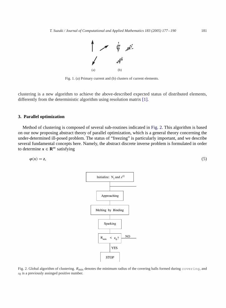
for r ∈ ��. Therefore, following the dipole hypothesis, it is appropriate to select distributed elementsclustered in narrow areas. This concept is illustrated inFig. 1. Since it is difficult to express our expectedstatus using an explicit cost function, we directly include the expected status into the proposed algorithmof clustering, where the primary current is reconstructed without prescribing the number of dipoles. Thus,


(a) (b)

Fig. 1. (a) Primary current and (b) clusters of current elements.

clustering is a new algorithm to achieve the above-described expected status of distributed elements,differently from the deterministic algorithm using resolution matrix[1].

3. Parallel optimization

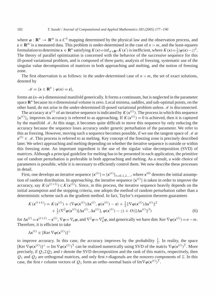
Method of clustering is composed of several sub-routines indicated inFig. 2. This algorithm is basedon our now proposing abstract theory of parallel optimization, which is a general theory concerning theunder-determined ill-posed problem. The status of “freezing” is particularly important, and we describeseveral fundamental concepts here. Namely, the abstract discrete inverse problem is formulated in orderto determinex ∈ Rm satisfying

�(x)= z, (5)

Fig. 2. Global algorithm of clustering.Rmin denotes the minimum radius of the covering balls formed duringcovering , and�0 is a previously assinged positive number.


where� : Rn → Rm is aC3 mapping determined by the physical law and the observation process, andz ∈ Rm is a measured data. This problem is under-determined in the case ofn>m, and the least-squaresformulation to determinex ∈ Rn satisfyingK(x)=inf x′∈RnK(x′) is inefficient,whereK(x)= 1

2|�(x)−z|2.The theory of parallel optimization is concerned with the behavior of the successive sequence for thisill-posed variational problem, and is composed of three parts; analysis of freezing, systematic use of thesingular value decomposition of matrices in both approaching and melting, and the notion of freezingzone.The first observation is as follows: in the under-determined case ofn>m, the set of exact solutions,

denoted by

M = {x ∈ Rn | �(x)= z},forms an (n–m)-dimensional manifold generically. It forms a continuum, but is neglected in the parameterspaceRn because itsndimensional volume is zero. Local minima, saddles, and sub-optimal points, on theother hand, do not arise in the under-determined ill-posed variational problem unlessM is disconnected.The accuracy atx(�) of an iterative sequence is indicated byK(x(�)). The process in which this sequence

{x(�)}� improves its accuracy is referred to as approaching. IfK(x(�))= 0 is achieved, then it is capturedby the manifoldM. At this stage, it becomes quite difficult to move this sequence by only reducing theaccuracy because the sequence loses accuracy under generic perturbation of the parameter. We refer tothis as freezing. However, moving such a sequence becomes possible, if we use the tangent space ofM atx(�) ∈ M. This process is referred to as melting. Key concept of the freezing zone is precisely describedlater.We select approaching andmelting depending on whether the iterative sequence is outside or withinthis freezing zone. An important ingredient is the use of the sigular value decomposition (SVD) ofmatrices.Although a principal guideline for melting has to be presented in each application, the primitiveuse of random perturbation is preferable in both approaching and melting. As a result, a wide choice ofparameters is possible, while it is necessary to efficiently control them.We now describe these processesin detail.First, one develops an iterative sequence{x(�)}= {x(�)}�=0,1,2,..., wherex(0) denotes the initial assump-

tion of random distribution. Inapproaching, the iterative sequence{x(�)} is taken in order to improve theaccuracy, sayK(x(�+1))�K(x(�)). Since, in this process, the iterative sequence heavily depends on theinitial assumption and the stopping criteria, one adopts the method of random perturbation rather than adeterministic scheme such as the gradient method. In fact, Taylor’s expansion theorem guarantees

K(x(�+1))=K(x(�))+ (∇�(x(�))�x(�),�(x(�))− z)+ 12‖∇�(x(�))�x(�)‖2

+ 12(∇2�(x(�))[�x(�),�x(�)],�(x(�))− z)+O(‖�x(�)‖3) (6)

for �x(�)=x(�+1)−x(�),∇�=∇x�, and∇2�=∇2x �, and generically we have dim Ker∇�(x(�))=n−m.

Therefore, it is efficient to take

�x(�) ∈ [Ker∇�(x(�))]⊥to improve accuracy. In this case, the accuracy improves by the probability1

2. In reality, the space[Ker∇�(x(�))]⊥ = Im∇�(x(�))T can be realized numerically using SVD of the matrix∇�(x(�))T. Moreprecisely, ifQ1Q2 andr denote the SVD decomposition and the rank of this matrix, respectively, thenQ1 andQ2 are orthogonal matrices, and only firstr-diagonals are the nonzero components of. In thiscase, the firstr column vectors ofQ1 form an ortho–normal basis of Im∇�(x(�))T.


This process of approaching is violated by the statefreezing, where the iterative sequence is capturedbyM. Again from (6), this is the case in which the accuracyK(x(�)) is extremely small in comparisonwith the mesh size‖�x(�)‖, say, as

‖∇�(x(�))‖ · ‖�(x(�))− z‖ ≈ (‖∇�(x(�))T∇�(x(�))‖ + ‖∇2�(x(�))‖‖�(x(�))− z‖)‖�x(�)‖,or

‖�x(�)‖ ≈ ‖∇�(x(�))T∇�(x(�))‖−1‖∇�(x(�))‖K(x(�))1/2.We refer to this area asfreezing zone. A practical method is to consider that the sequence is in the

freezing zone when its accuracy is not improved despite several trials. This situation of freezing is brokenby using the tangent spaceTx(�)M. This is referred to asmelting, where the sequence is moved withoutlosing accuracy to a large extent by taking�x(�) ∈ Tx(�)M. In reality, we haveK(x(�))>1 and henceTx(�)M ≈ Ker∇�(x(�)). This approximation is justified again by (6), namely,K(x(�)) does not changeconsiderably in the case of�x(�) ∈ Ker∇�(x(�)). The SVD of∇�(x(�)) can be used for this purposealso. In fact, sinceQT2

TQT1 andr denote the SVD decomposition and the rank of thism × n matrix,respectively, the lastn–r column vectors ofQ1 form an ortho–normal basis of Ker∇�(x(�)).In this way, approaching and melting can be executed in a unified way, considering the freezing zone.

We refer to this method as the method of parallel optimization by random perturbations, i.e.,�x(�) istaken randomly in Im∇�(x(�))T and Ker∇�(x(�)) according to

‖�x(�)‖> ‖∇�(x(�))T∇�(x(�))‖−1‖∇�(x(�))‖K(x(�))1/2and

‖�x(�)‖< ‖∇�(x(�))T∇�(x(�))‖−1‖∇�(x(�))‖K(x(�))1/2,respectively, where the SVDs of∇�(x(�))T and∇�(x(�)) are used. Sometimes the iterative sequencedigresses from the freezing zone after several meltings, and then the approaching sets up automatically.A practical method is to adopt a uniform mesh size = ‖�x(�)‖ for �= 0,1,2, . . . and is to consider thatthe sequence is in the freezing zone if its accuracy is approximately the one at the first freezing.In each application a customized strategy has to be developed in melting. If the unknown parameterx

represents the state of the distributed elements, then the method ofclusteringmakes it possible to clusterthem into several narrow areas. This is achieved by adjusting the approximate outer measures of thecounting measure in accordance with the clustering degree of the elements, and we shall describe themin the context of the MEG data analysis, where�(x) is given by (4).With regard to the leading principle,binding is taken into consideration. Let us considerx(�) =

(Q(�), a�) ∈ FN as being in the freezing zone and assignS� = {a(�)k | k = 1, . . . , N} ⊂ �. Then,upon considering small�>0, random open balls are provided, satisfying

S� ⊂Mcov⋃i=1

B(bi , �),

whereMcov denotes the number of balls andB(bi , �) = {a ∈ R3 | ‖a − bi‖< �}. This is repeated untila minimal numberMcov of covering balls is achieved. We refer to this process ascovering. Once suchcovering balls are obtained, then newbi and � are introduced, making each ballB(bi , �) as small as


possible up to the mesh size without losing any of the elements within. The resulting ball is denoted byB(b′

i , �i), and thus, it holds that

S� ⊂Mcov⋃i=1

B(b′i , �i) and min

a(�)k ∈B(bi ,�)‖�a(�)i ‖< �i < �.

We refer to this process asbiting. If this is achieved, then, we considermelting forx(�) under the constraint

S�+1 ⊂Mcov⋃i=1

B(b′i , �i). (7)

In the other sub-routine,sparking, the number of elements is decreased, namely, the number of elementsof x(�), denoted byN = N�, does not change in binding, but the sparking realizesN�+1<N�. The firstsparking delates a current element when the magnetic field generated by it is sufficiently small, namely,one examines‖Q(�)

k ‖ (k= 1, . . . , N�), and delatesx(�)k if it is smaller than the mesh size,‖�Q(�)k ‖. In the

second sparking, the elements in a covering ball, denoted byB(bi , �), are replaced with their algebraicsum if the ball can be shrunk with the radius smaller than the mesh size, max

a(�)k ∈B(bi ,�)‖�a(�)k ‖. Thisprocess is different from approaching or melting, and maintaining accuracy has to be sufficiently takeninto consideration.In contrast withMUSIC[10], method of clustering uses single time sliced data to determine the number

and the location of dipoles, and therefore, it is applicable to several inverse problems for an unknownnumber of sources without using time series analysis. Among them is the localization of the acousticsource.

4. Approaching and melting in detail

In approaching, the number of elements does not change;N� =N . For simplicity, we takex′ = x(�+1),x = x(�), �x = x′ − x, andxk = (Qk, ak) = x(�)k for the iterative sequence in such a state. Then, we canrepresent∇�(x) as

∇�(x)= [DQ1 (x),Da1(x), . . . , . . . ,DQN(x),DaN(x)],

whereDQk (x) andDak(x) arem× 3 matrices defined by

DQk (x)=[

��i(x)

�Qkj

]and Dak(x)=

[��i(x)

�akj

]

for

�j (x)=N∑k=1

�04�

Qk × (pj − ak)

|pj − ak|3 · n(pj ).


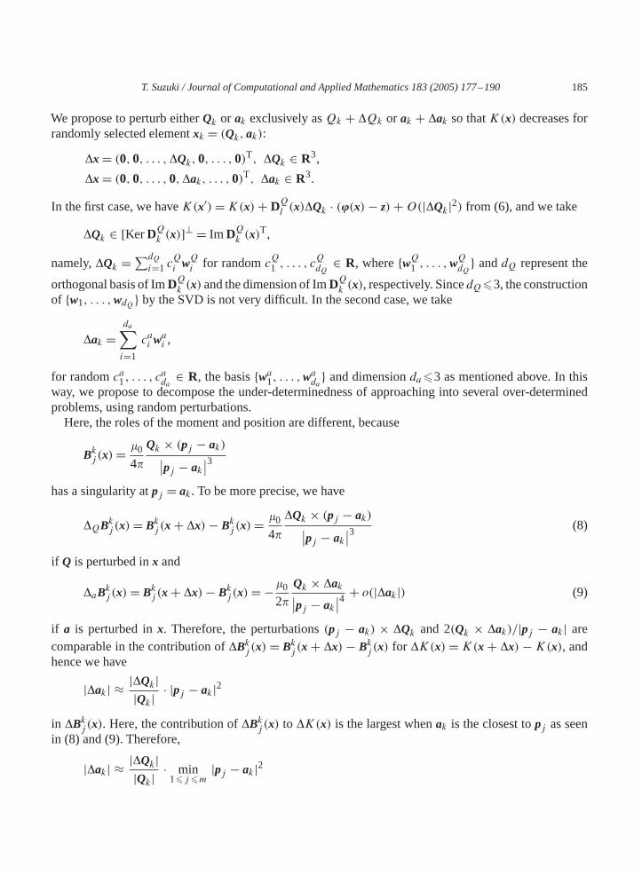
We propose to perturb eitherQk or ak exclusively asQk + �Qk or ak + �ak so thatK(x) decreases forrandomly selected elementxk = (Qk, ak):

�x = (0,0, . . . ,�Qk,0, . . . ,0)T, �Qk ∈ R3,

�x = (0,0, . . . ,0,�ak, . . . ,0)T, �ak ∈ R3.

In the first case, we haveK(x′)=K(x)+ DQl (x)�Qk · (�(x)− z)+O(|�Qk|2) from (6), and we take�Qk ∈ [KerDQk (x)]⊥ = ImDQk (x)

T,

namely,�Qk =∑dQi=1 c

Qi wQi for randomc

Q1 , . . . , c

QdQ

∈ R, where{wQ1 , . . . ,wQdQ} anddQ represent theorthogonal basis of ImDQk (x) and the dimension of ImD

Qk (x), respectively. SincedQ�3, the construction

of {w1, . . . ,wdQ} by the SVD is not very difficult. In the second case, we take

�ak =da∑i=1

cai wai ,

for randomca1, . . . , cada

∈ R, the basis{wa1, . . . ,wada } and dimensionda�3 as mentioned above. In thisway, we propose to decompose the under-determinedness of approaching into several over-determinedproblems, using random perturbations.Here, the roles of the moment and position are different, because

Bkj (x)= �04�

Qk × (pj − ak)∣∣pj − ak∣∣3

has a singularity atpj = ak. To be more precise, we have

�QBkj (x)= Bkj (x + �x)− Bkj (x)= �04�

�Qk × (pj − ak)∣∣pj − ak∣∣3 (8)

if Q is perturbed inx and

�aBkj (x)= Bkj (x + �x)− Bkj (x)= −�02�

Qk × �ak∣∣pj − ak∣∣4 + o(|�ak|) (9)

if a is perturbed inx. Therefore, the perturbations(pj − ak) × �Qk and 2(Qk × �ak)/|pj − ak| arecomparable in the contribution of�Bkj (x) = Bkj (x + �x) − Bkj (x) for �K(x) = K(x + �x) − K(x), andhence we have

|�ak| ≈ |�Qk||Qk|

· |pj − ak|2

in �Bkj (x). Here, the contribution of�Bkj (x) to �K(x) is the largest whenak is the closest topj as seenin (8) and (9). Therefore,

|�ak| ≈ |�Qk||Qk|

· min1�j �m

|pj − ak|2


follows, and in particular, elements{Qk�(x − ak)} near{p1, . . . , pm} are difficult to move. This difficultyis avoided by the weighted random perturbation, more precisely, when the random perturbations of themoments and positions are considered as 1 vs.[(|�ak||Qk|)/|�Qk|]minj |pj − ak|−2. This process isreferred to asbiasing. Without such a weight, to cluster elements in narrow areas is not easy, becausethe binding just takes care of their positions. A practical method is to take|�ak| ≈ |�Qk| and adopt 1:1weight always.Another issue met in approaching is as follows. We have�QBkj · n(pj )= 0 and�aBkj · n(pj )= o(1) if

Qk andpj − ak are parallel ton(pj ). In other words, such an element does not change the accuracy to alarge extent under the small perturbation, and therefore, is difficult to move. Similarly, the contributionof �Bkj (x) to reduceK(x) is maximum if�Qk and�ak are perpendicular ton(pj ), and therefore, ifn(pj ),pj − ak, andQk are perpendicular to a vector that is very close topj , then it is also difficult to avoid thissituation in approaching. These states are referred to asdegenerateandlooping holes, respectively, andsuch silent elements are moved mainly in melting. Following numerical experiments, for the degeneratehole, it is efficient not to reduce the radius of the covering ball in biting below two or three times themesh size, and also to avoid a covering ball containing only one element. On the other hand, falling intothe looping hole can be avoided by the sparking described above and the under-determined quantizationdescribed below.Inbinding, the iterativesequence{x(�)} is ledwithahighaccuracy to formasetof clusteredelements. Let

us consider the covering as being performedwith the covering balls denoted byB(bi , �) (i=1, . . . ,Mcov).Put

Ai = {ak | ak ∈ B(bi , �)}and let the number of elements inAi bedi . Since treating all elements at each step makes the bindingdifficult, we propose to execute themelting to elementswithin a randomely selected covering ballB(bi , �).Sometimes, it is done under the constraint

ak + �ak ∈ B(b′i , �i) for all ak ∈ Ai (10)

instead of (7), which means that this random perturbation is adopted only when (10) is satified, and ifthis is not the case one more trial of random perturbation is done. Then, the case 6di�m can occur ifB(bi , �) contains few elements, wheredi denotes the number of elements insideB(b′

i , �i). The problemof taking�x ∈ Ker∇�(x) then becomes over-determined and such a selection is difficult. To avoid thisissue, randomdi channels can be selected withdi�di , to use the restricted data. This process is referred toas theunder-determined quantization. Namely, we use randomly decomposed data through several stepsof iteration. This sub-routine of under-determined quantization is set up when the number of coveringballs does not change after several steps of binding.

5. Numerical examples

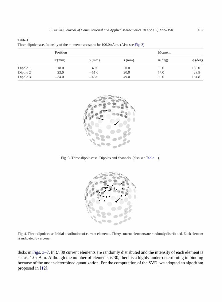
We cite the 3-dipole numerical experiment (Table 1andFig. 3). In this example, numerically computed�(x) is consideredas themeasureddatum for thepresumed threedipoles(a1,Q1), (a2,Q2), (a3,Q3) ∈ R6,i.e.,x = (a,Q) ∈ R18 for a= (a1, a2, a3),Q= (Q1,Q2,Q3) indicated by the three arrows inFig. 3. Uponthe actual MRI mapping of a subject, we approximate the brain� by a ball with a radius of 85.0mm.Following the actual MEG device and MRI data, we set up 160 channels on�� that are indicated by gray


Table 1Three-dipole case. Intensity of the moments are set to be 100.0 nAm. (Also seeFig. 3)

Position Moment

x (mm) y (mm) z(mm) � (deg) � (deg)

Dipole 1 −18.0 49.0 20.0 90.0 180.0Dipole 2 23.0 −51.0 20.0 57.0 28.8Dipole 3 −34.0 −46.0 49.0 90.0 154.8

Fig. 3. Three-dipole case. Dipoles and channels. (also seeTable 1.)

Fig. 4. Three-dipole case. Initial distribution of current elements. Thirty current elements are randomly distributed. Each elementis indicated by a cone.

disks inFigs. 3–7. In�, 30 current elements are randomly distributed and the intensity of each element isset as, 1.0nAm. Although the number of elements is 30, there is a highly under-determining in bindingbecause of the under-determined quantization. For the computation of the SVD, we adopted an algorithmproposed in[12].


Fig. 5. Three-dipole case. Transient state.

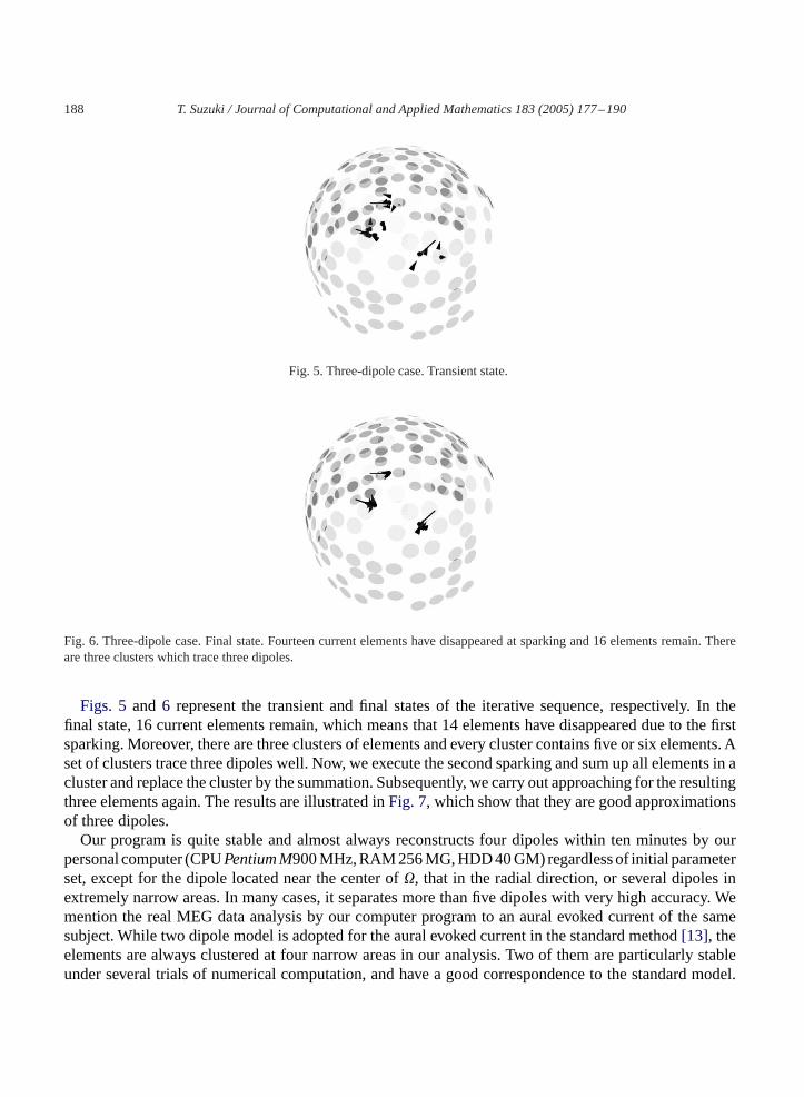
Fig. 6. Three-dipole case. Final state. Fourteen current elements have disappeared at sparking and 16 elements remain. Thereare three clusters which trace three dipoles.

Figs. 5and6 represent the transient and final states of the iterative sequence, respectively. In thefinal state, 16 current elements remain, which means that 14 elements have disappeared due to the firstsparking. Moreover, there are three clusters of elements and every cluster contains five or six elements. Aset of clusters trace three dipoles well. Now, we execute the second sparking and sum up all elements in acluster and replace the cluster by the summation. Subsequently, we carry out approaching for the resultingthree elements again. The results are illustrated inFig. 7, which show that they are good approximationsof three dipoles.Our program is quite stable and almost always reconstructs four dipoles within ten minutes by our

personal computer (CPUPentiumM900MHz,RAM256MG,HDD40GM) regardlessof initial parameterset, except for the dipole located near the center of�, that in the radial direction, or several dipoles inextremely narrow areas. In many cases, it separates more than five dipoles with very high accuracy. Wemention the real MEG data analysis by our computer program to an aural evoked current of the samesubject. While two dipole model is adopted for the aural evoked current in the standard method[13], theelements are always clustered at four narrow areas in our analysis. Two of them are particularly stableunder several trials of numerical computation, and have a good correspondence to the standard model.


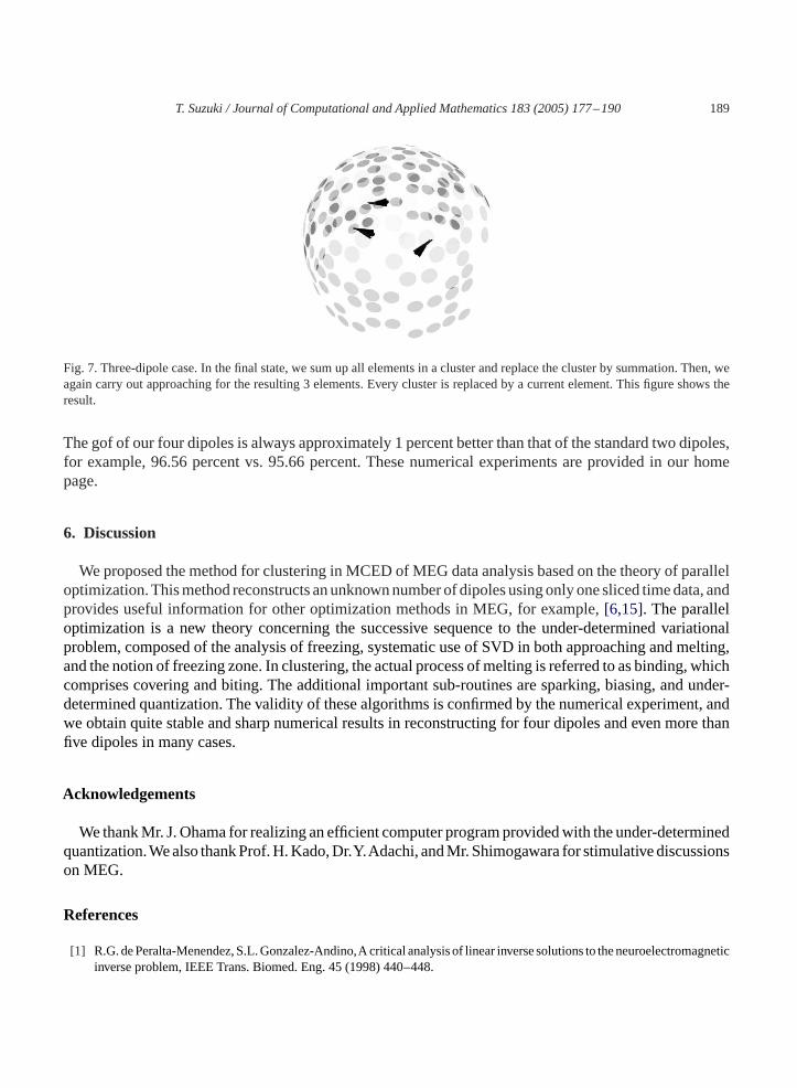
Fig. 7. Three-dipole case. In the final state, we sum up all elements in a cluster and replace the cluster by summation. Then, weagain carry out approaching for the resulting 3 elements. Every cluster is replaced by a current element. This figure shows theresult.

The gof of our four dipoles is always approximately 1 percent better than that of the standard two dipoles,for example, 96.56 percent vs. 95.66 percent. These numerical experiments are provided in our homepage.

6. Discussion

We proposed the method for clustering in MCED of MEG data analysis based on the theory of paralleloptimization.Thismethod reconstructs anunknownnumberof dipolesusingonly onesliced timedata, andprovides useful information for other optimization methods in MEG, for example,[6,15]. The paralleloptimization is a new theory concerning the successive sequence to the under-determined variationalproblem, composed of the analysis of freezing, systematic use of SVD in both approaching and melting,and the notion of freezing zone. In clustering, the actual process ofmelting is referred to as binding, whichcomprises covering and biting. The additional important sub-routines are sparking, biasing, and under-determined quantization. The validity of these algorithms is confirmed by the numerical experiment, andwe obtain quite stable and sharp numerical results in reconstructing for four dipoles and even more thanfive dipoles in many cases.

Acknowledgements

We thankMr. J.Ohama for realizing an efficient computer programprovidedwith the under-determinedquantization.Wealso thankProf.H.Kado,Dr.Y.Adachi, andMr.Shimogawara for stimulativediscussionson MEG.

References

[1] R.G.dePeralta-Menendez,S.L.Gonzalez-Andino,Acritical analysis of linear inversesolutions to theneuroelectromagneticinverse problem, IEEE Trans. Biomed. Eng. 45 (1998) 440–448.


[2] D.B. Geselowitz, On bioelectric potentials in an inhomogeneous volume conductor, Biophys. J. 7 (1967) 1–11.[3] D.B.Geselowitz, On themagnetic field generated outside an inhomogeneous volume conductor by internal current sources,

IEEE Trans. Magn. Mag. 6 (1970) 346–347.[4] F. Grynszpan, D.B. Geselowitz, Model studies of the magnetocardiogram, Biophys. J. 13 (1973) 911–925.[5] M. Hämäläinen, R. Hari, R.J. Ilmoniemi, J. Knuutila, O.V. Lounasmaa, Magnetoencephalography—theory,

instrumentation, and applications to noninvasive studies of the working human brain, Rev. Modern Phys. 65 (1993)413–515.

[6] M. Huang, C.J. Aine, E.R. Flynn, Multi-start downhill simplex method for spatio-temporal source localization inmagnetoencephalography, Electroen. Clin. Neurophysiol. 108 (1998) 32–44.

[7] H. Kado, H. Ogata, Y. Haruta, M. Higuchi, M. Shimogawara, J. Kawai, A. Adachi, C. Bertrand, G. Uehara, The imagingof a magnetic source, in: T. Furukawa (Ed.), Biological Imaging and Sensing, Springer, Berlin, 2004, pp. 117–204.

[8] K. Matsuura,Y. Okabe, Selective minimum-norm solution of the biomagnetic inverse problem, IEEE Trans. Biomed. Eng.42 (1995) 608–615.

[9] J.C. Mosher, R.M. Leahy, Recursive MUSIC: a framework for EEG and MEG source localization, IEEE Trans. Biomed.Eng. 45 (1998) 1342–1354.

[10] J.C. Mosher, P.C. Lewis, R.M. Leahy, Multiple dipole modeling and localization from spatio-temporal MEG data, IEEETrans. Biomed. Eng. 39 (1992) 541–557.

[11] R.D.Pascual-Marqui, C.M.Michel, D. Lehmann, Low resolution electromagnetic tomography: a newmethod for localizingelectrical activity in the brain, Internat. J. Psychophysiol. 18 (1994) 49–65.

[12] W.H. Press, B.P. Flannery, S.A. Teukolski, W.T. Vetterling, Numerical Recipes in C, Cambridge University Press,Cambridge, 1988.

[13] J. Sarvas, Basic mathematical and electromagnetic concepts of the biomagnetic inverse problem, Phys. Med. Biol. 32(1987) 11–22.

[14] M. Scherg, D. von Cramon, Two bilateral sources of the late AEP as identified by a spatio-temporal dipole model, Elec.Clin. Neurol. 62 (1985) 32.

[15] K. Uutela, M. Hämäläinen, R. Salmelin, Global optimization in the localization of neuromagnetic sources, IEEE Trans.Biomed. Eng. 45 (1998) 716–723.

[16] J.Wang, S.J.Williamson, L. Kaufman, Magnetic source images determined by a lead-field analysis: the unique minimum-norm least-squares estimation, IEEE Trans. Biomed. Eng. 39 (1992) 665–675.

Documents

Parallel optimization applied to magnetoencephalography