Parallel Mesh Refinement with Optimal Load Balancing

Jean-Francois Remacle, Joseph E. Flaherty and Mark. S. Shephard

Scientific Computation Research Center

Scope of the presentation

• The Discontinuous Galerkin Method (DGM)– Discontinuous Finite Elements– Spatial discretization– Time discretization– DG for general conservation laws

• Adaptive parallel software– Adaptivity– Parallel Algorithm Oriented Mesh Datastructure

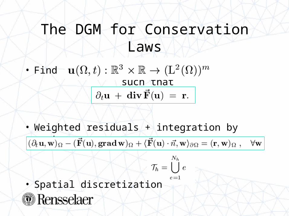
The DGM for Conservation Laws

• Find such that

• Weighted residuals + integration by parts

• Spatial discretization

The DGM for Conservation Laws

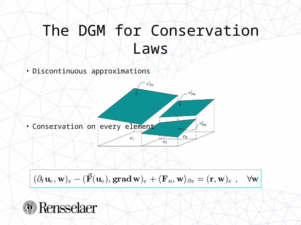
• Discontinuous approximations

• Conservation on every element

The DGM for Conservation Laws

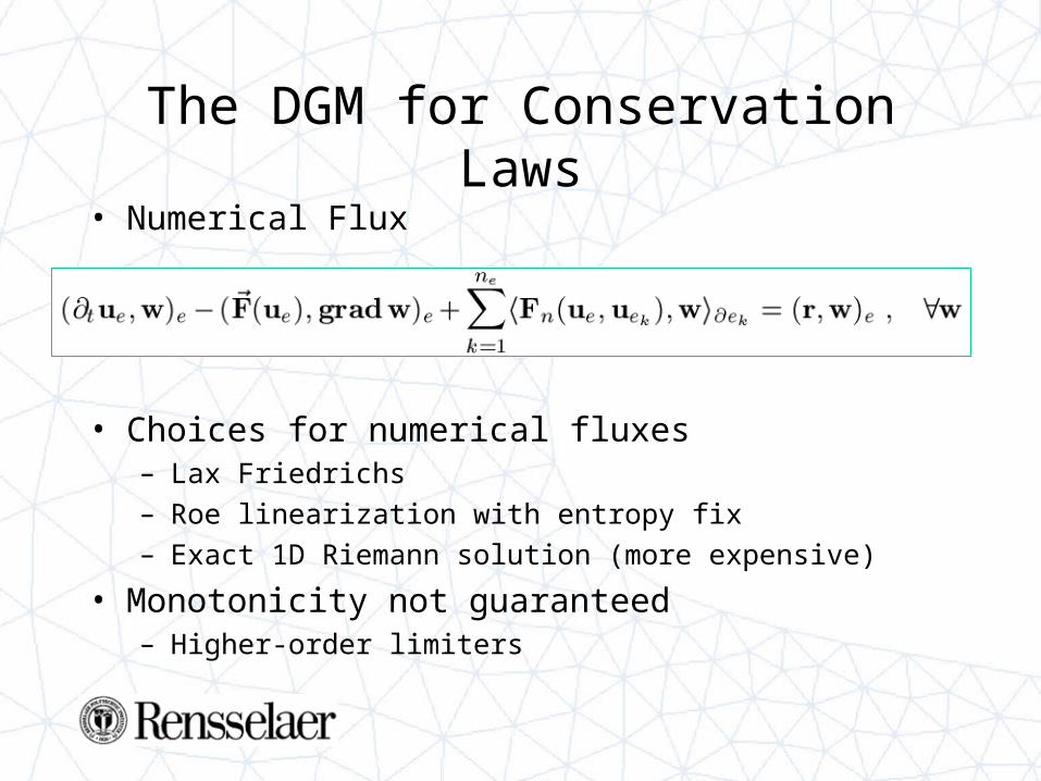
• Numerical Flux

• Choices for numerical fluxes– Lax Friedrichs – Roe linearization with entropy fix– Exact 1D Riemann solution (more expensive)

• Monotonicity not guaranteed– Higher-order limiters

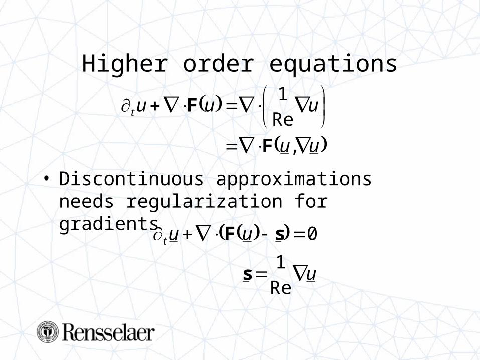
Higher order equations

• Discontinuous approximations needs regularization for gradients

uu

uuut

,

Re1

F

F

u

uut

Re1

0

s

sF

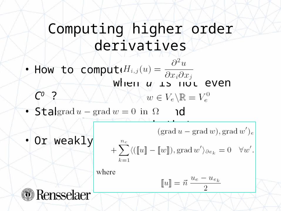
Computing higher order derivatives

• How to compute when u is not even C0 ?

• Stable gradients : find such that

• Or weakly

Computing higher order derivatives

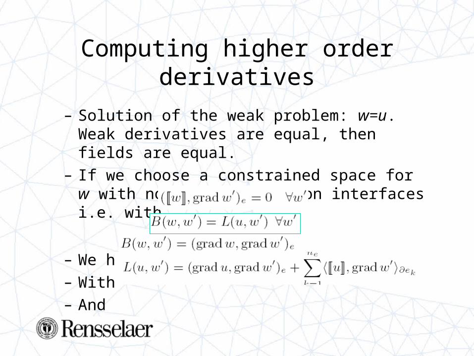
– Solution of the weak problem: w=u. Weak derivatives are equal, then fields are equal.

– If we choose a constrained space for w with no average jumps on interfaces i.e. with

– We have– With– And

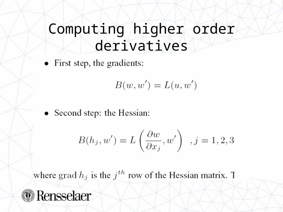
Computing higher order derivatives

– For higher order derivatives:

Time discretization

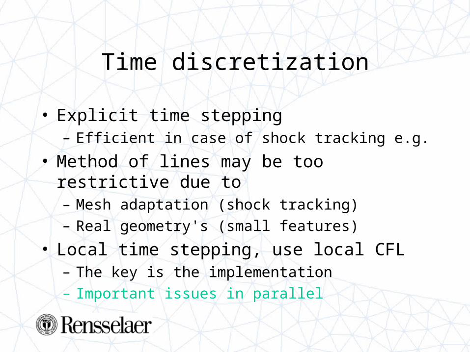
• Explicit time stepping– Efficient in case of shock tracking e.g.

• Method of lines may be too restrictive due to– Mesh adaptation (shock tracking)– Real geometry's (small features)

• Local time stepping, use local CFL– The key is the implementation– Important issues in parallel

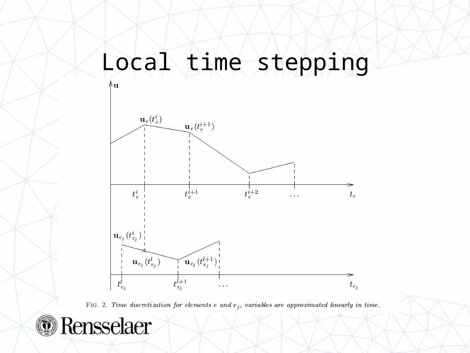
Local time stepping

Local time stepping

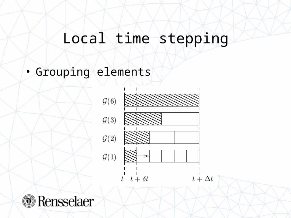
• Grouping elements

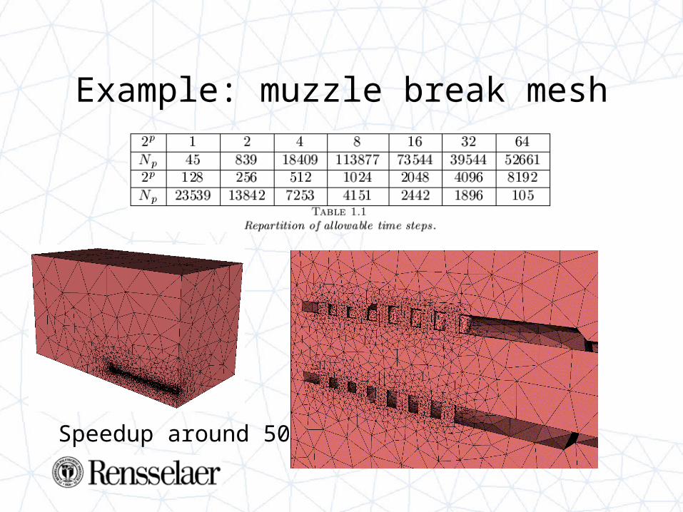
Example: muzzle break mesh

Speedup around 50

Parallel Issues

• Good practice in parallel– Balance the load between processors– Minimize communications/computations– Alternate communications and computations

• Local time stepping– Elementary load depends on local CFL– Not the mostly critical issue

Parallel issues

• Example, load is balanced when– Proc 0 : 2000(1dt) + 1000 (2dt) – Proc 1 : 3000(1dt) + 500 (2dt)– Total Load : 4000 dt

• If synchronization after every sub-time steps– Proc 0 waits 1000 dt at the first sync.– Proc 1 waits 1000 dt at the first sync– Maximum parallel speedup = 4/3

Parallel issues

• Solution– Synchronization only after the goal time step– Non blocking sends and receive after each sub-

time step– Inter-processor faces store the whole history– Some elements may be “retarded”

A Parallel Algorithm Oriented Datastructure

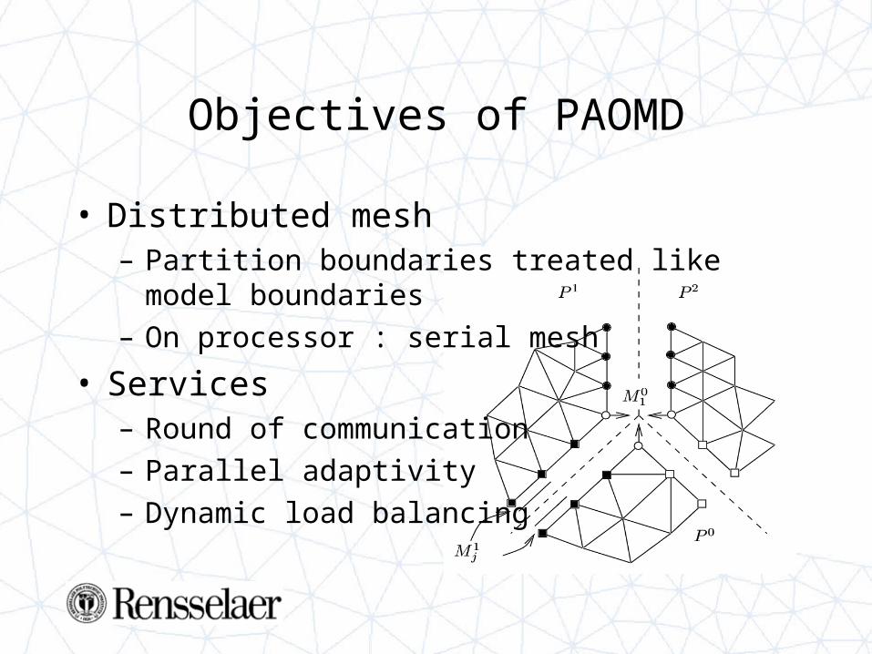
Objectives of PAOMD

• Distributed mesh– Partition boundaries treated like model boundaries– On processor : serial mesh

• Services– Round of communication– Parallel adaptivity– Dynamic load balancing

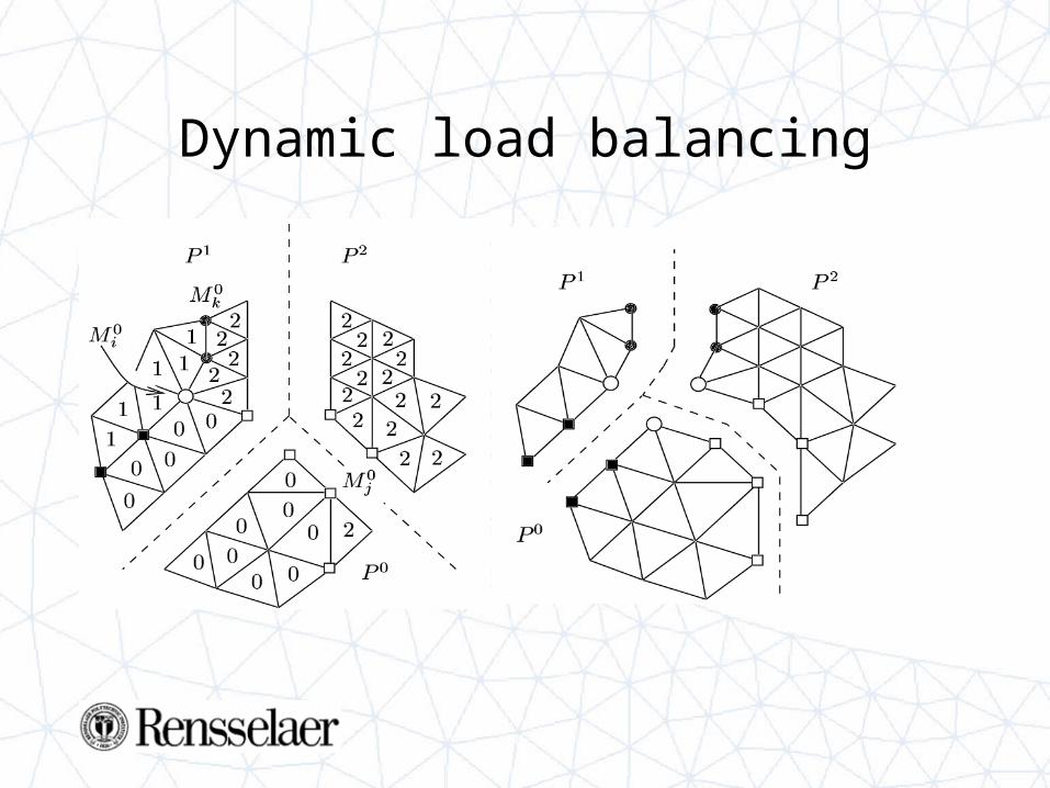
Dynamic load balancing

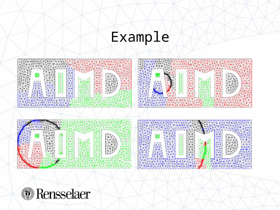
Example

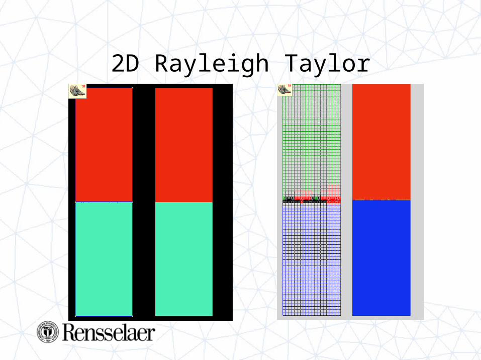
2D Rayleigh Taylor

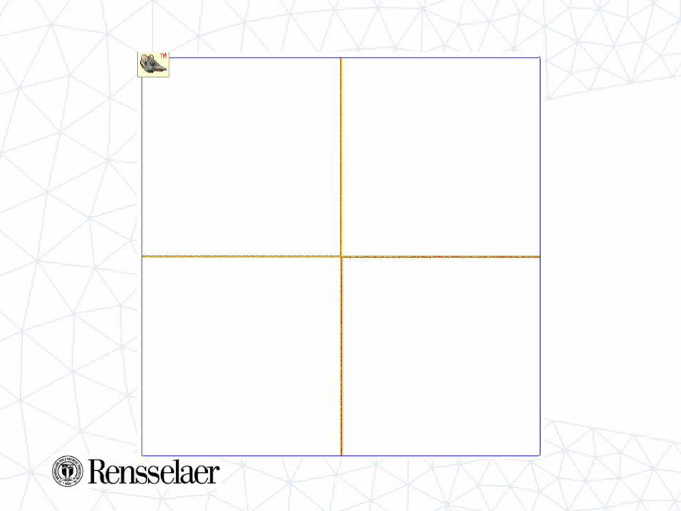
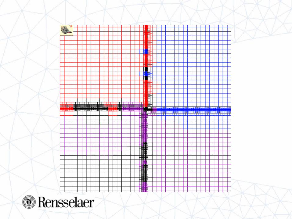
Four contacts

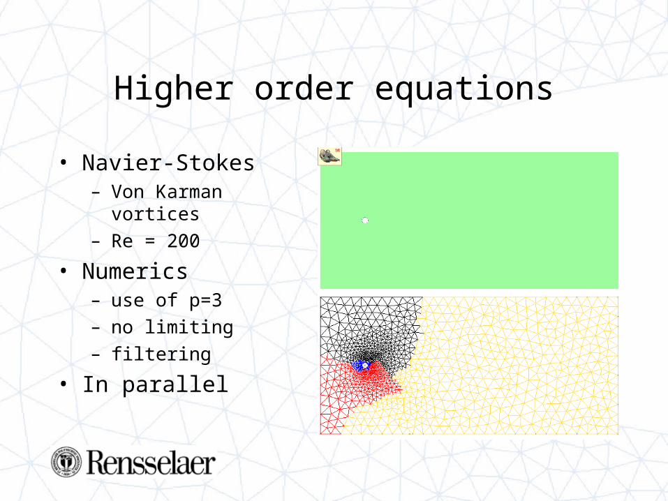
Higher order equations

• Navier-Stokes– Von Karman vortices– Re = 200

• Numerics– use of p=3– no limiting– filtering

• In parallel

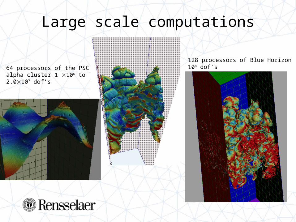
64 processors of the PSC alpha cluster 1 106 to 2.0107 dof’s

128 processors of Blue Horizon108 dof’s

Large scale computations

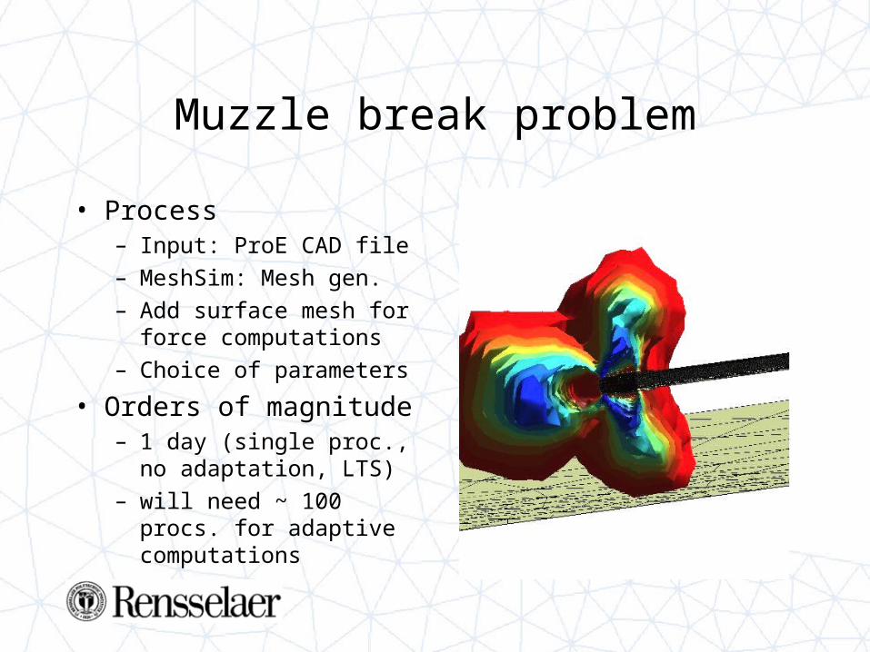
Muzzle break problem

• Process– Input: ProE CAD file– MeshSim: Mesh gen.– Add surface mesh for

force computations– Choice of parameters

• Orders of magnitude– 1 day (single proc., no

adaptation, LTS)– will need ~ 100 procs. for

adaptive computations

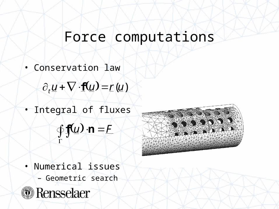
Force computations

• Conservation law

• Integral of fluxes

• Numerical issues– Geometric search

)(uruut f

Fu

nf

2D computations

• Importance of – adaptivity– 2nd order method

• Influence of the muzzle

2D computations

3D computations

• Challenging– Large number of dof’s– Complex geometry

Discussion

• The issue– Large scale computations– Explicit time stepping, – Load balancing

• In progress– Semi implicit and implicit schemes– Higher order limiters improved