Parallel GCD and some related parallel computations over ... · Then, we may easily solve the gcd, lcm, Padt, and Berlekamp-Massey problems at the latter (randomized) cost for p >

ELSEVIER Theoretical Computer Science 162 (1996) 173-223

Theoretical Computer Science

Parallel some related

computation of polynomial parallel computations over

Victor Y. Pan *

GCD and abstract fields ’

Department of Mathematics and Computer Science, Lehman College, City University of New York, Bronx, NY 10468, USA

Abstract

Several fundamental problems of computations with polynomials and structured matrices are well known for their resistance to effective parallel solution. This includes computing the gcd, the

lcm, and the resultant of two polynomials, as well as any selected entry of either the extended Euclidean scheme for these polynomials or the Padt? approximation table associated to a fixed power series, the solution of the Berlekamp-Massey problem of recovering the n coefficients of a linear recurrence sequence from its first 2n terms, the solution of a Toeplitz linear system of

equations, computing the ranks and the null-spaces of Toeplitz matrices, and several other computations with Toeplitz, Hankel, Vandermonde, and Cauchy (generalized Hilbert) matrices and with matrices having similar structures. Our algorithms enable us to reach new record estimates

for randomized parallel arithmetic complexity of all these computations (over any field of constants), that is, O((logn)h) time and O((n’ log logn)/(logn)h-Y) arithmetic processors, where n

is the input size, g varies from 1 to 2, and h varies from 2 to 4, depending on the computational problem and on the fixed field of constants. The estimates include the cost of correctness tests for the solution. The results have further applications to many related computations over abstract fields and rely on some new techniques (in particular, on recursive Pad& approximation and regularization of Pad& approximation via randomization), which might be of some independent technical interest. In particular, an auxiliary algorithm computes (over any field) the coefficients of a polynomial from the power sums of its zeros, which is an important problem of algebraic coding.

1. Introduction

1.1. Our subject

Fundamental computations with Toeplitz, Hankel, Toeplitz-like, and Hankel-like ma-

trices (generalizing Toeplitz and Hankel matrices) as well as with some other dense

* Internet: [email protected]. ’ The results of this paper have been presented at the 7th Annual ACM-SIAM Symposium on Discrete Algorithms, in Atlanta, Georgia, in January 1996; the author is greatful to ACM and SIAM for permission

to cite them.

SO304-3975/96/$15.00 @ 1996 -Elsevier Science B.V. All rights reserved

PfI SO304-3975(96)00030-S

174 V. Y. PanITheoretical Computer Science 162 (1996) 173-223

and structured matrices are among the major topics of computations in linear algebra

(for definitions, see Section 2 or [61] and [12]). These computations include solving

nonsingular and singular linear systems of equations with dense and structured coeffi-

cient matrices V, computing the ranks of such matrices, their null-spaces, determinants,

and inverses (where det V # 0).

The algorithms for these problems have numerous extensions and applications. In par-

ticular, in Section 12, we consider extensions to the celebrated problems of computing

the greatest common divisor (gcd), the least common multiple (lcm), the resultant, and

all the entries of the extended Euclidean scheme for a pair of univariate polynomials,

of computing a fixed entry of the Pad& table for a given formal power series, and

of recovering the n coefficients of a linear recurrence sequence from its first 2n terms

(known as the Berlekamp-Massey problem). In Sections 2 and 12, we will recall some

reductions of these problems to Toeplitz and/or Toeplitz-like computations and their

correlations to each other; this material can be found in [17, 15,32, 121 as well (also

compare [25, IS]). In particular, Facts 12.1 and 12.2 of Section 12 enable us to reduce

the gcd problem at first to solving a simple polynomial identity and then, further, to

Toeplitz-like computations, namely, to computing the rank of a Sylvester (resultant)

matrix and to solving a nonsingular (resultant or subresultant) linear system of equa-

tions. Alternatively, the gcd problem can easily be reduced to computing an entry of

a Pad& table for the formal power series defined by the quotients of 2 polynomials

u(x)/v(x) or u( l/x)/u( l/x) (see our Appendix A), and this problem is equivalent to the

rank computation and linear system solving problems for Toeplitz input matrices (cf.

[17] or [12]). Due to these and other known reductions, we will focus on Toeplitz and

Toeplitz-like computations, in particular, on the rank computation and linear system

solving.

We will conclude this subsection with recalling about some further major applica-

tions of Toeplitz-Hankel-type computations to the theory and practice of computing

for sciences, engineering, and communication. They include applications to shift reg-

ister synthesis, BCH and Read-Solomon decoding of error-correcting codes, inverse

scattering, adaptive filtering, modelling of stationary and nonstationary processes, nu-

merical computations for Markov chains, sparse multivariate polynomial interpolation,

solution of partial differential and integral equations, parallel computations with gen-

eral matrices over an arbitrary field of constants, and approximating polynomial zeros

[5,18, 19,25,36,53,40, 17,51,52,20,37,46,62,64,47,73, 12,82,69].

1.2. Model of computation

We will be looking for fast and processor efficient parallel algorithms for the listed

computational problems. Stating our complexity estimates, we will assume the cus-

tomary EREW PRAM model of parallel computing [30,50,35], under which, at every

time-step, each nonidle processor may perform a single unit cost operation (in our case,

arithmetic operation or a comparison with 0). In fact, to obtain our upper estimates for

the cost of performing our algorithms over the complex field of constants, we essen-

V. Y. PanITheoretical Computer Science 162 (1996) 173-223 175

tially need just a model that supports performing fast Fourier transform at the nth roots

of 1 by using O(logn) time on n processors, and this can be achieved, for instance, on

the butterfly, shuffle-exchange, or hypercube processor arrays [87,75]. Over an arbitrary

field of constants, our cornerstone operation will be polynomial multiplication modulo

x”, which can be performed by using O(logn) time and O(n loglogn) processors (cf.

[21]) under various realistic computer models too.

Hereafter, we will write O(t, p) in order to denote simultaneous upper bounds O(t)

on time and O(p) on the number of processors used. We will assume a variant of

Brent’s scheduling principle [16], according to which a single processor may simulate

one step of s processors in O(s) steps, so that O(t, p) implies O(tp, 1 ), but not neces-

sarily vice versa. The product w = tp of parallel time and the number of processors

used by a parallel algorithm is called its potential work [50,71]. The algorithm is

called work (or processor) ejicient if it supports the bound O((logn)d) on the work

inejhciency ratio w(n)/&(n), where n is the input size, w(n) is the work of this algo-

rithm, tseq(n) is the current record sequential time for the solution of the same problem,

and d is a constant, independent of n. If the ratio remains O((logn)d) even when we

replace the current record a,,(n) by a known lower bound on the sequential time, the

algorithm is called strongly work (or processor) ejicient. An algorithm is in NC if

its parallel time is O((logn)d) and if its work and processor bounds are O(n) for 2

constants c and d, independent of n. RNC stands for randomized NC; the randomized

estimates for the computational cost are of Las Vegas type, if they include the cost

of testing correctness of the output, and of Monte Carlo type, otherwise. Devising

algorithms that would be both in NC or RNC and work efficient turned out to be a

quite difficult task for the computational problems cited in the previous subsection.

1.3. Fast sequential solution and its parallel acceleration based on algorithms

for computations with general matrices

The sequential time bound

t,,,(n) = O((log n)’ n log log n) (1.1)

is obtained (over any field of constants) for the gcd, lcm, Pad6 and Berlekamp-Massey

problems of size n, due to their solution by means of a fast version of the Euclidean

algorithm [l, 171, where the extra factor loglogn is the (small) price for using fast

polynomial multiplication over any field of constants [21]. The same sequential time

bound, for solving a nonsingular Toeplitz or Toeplitz-like linear system of n equa-

tions, has been supported by the algorithms of [ 171 for a Toeplitz system and of

[43,44] for a Toeplitz-like system, the latter algorithm relies on [14,54] (cf. also

[55,28,2,24,34]). All these fast sequential algorithms, however, resist their effective

parallelization. Moreover, for some time, the only known way to obtain NC algorithms

for the above-computational problems was by first reducing each of these problems to

solving O(n) nonsingular Toeplitz or Toeplitz-like systems, each of n equations [here-

after referred to as LIN . SOLVE . T(n)] ( corn are p Sections 2 and 12 and [15,32])

176 V. Y. Pan I Theoretical Computer Science 162 (1996) 173-223

and then by applying the known fast parallel algorithms available for solving a general

nonsingular linear system of equations [27,74,6,22,3 11. The latter algorithms support

deterministic cost bounds O((log n)2, nW+O ), where w 3 2 is the exponent of matrix mul-

tiplication, whose current record upper bound is w < 2.375... and where (T varies from

i [74] or slightly less than i [31] (over fields of characteristics p = 0 and p > n) to 1

(over any field [6,22]).

The time bound 0((logn)2) is quite attractive, but the processor and work bounds

of order nw+O for a single linear system are clearly too high, in comparison with ( 1.1).

1.4. A solution over the fields of characteristics 0 and greater than n

Over the fields of characteristics p = 0 and p > n, the algorithm of [63] yields the

bounds

c, = O((log ?z)2, (n2 log log n)/ logn) (1.2)

on the parallel cost and w(n)/&(n) = 0( n on the work efficiency ratio for LIN . ) SOLVE . T(n). For an n x n Toeplitz-like matrix V and a vector f; the algorithm com-

putes the Krylov sequence { Vif) and the values {trace (Vi)}, i = 0, 1, . . . , m, m = O(n), at the cost C,, of (1.2), over any field of constants. Given the traces of Yi, a simple

and elegant algorithm of [78] (see our Section 3) computes the coefficients of Cv(x),

the characteristic polynomial of V, at the cost O((logn)2,(n2 loglogn)/logn), over the

fields of characteristics p = 0 and p > n. Given CV(X), one easily obtains det V, and if

det Y # 0, then also V-’ and V-iJ all at the cost C,, of (1.2). If p = 0, then, within

the same deterministic cost bound C,, of (1.2), the algorithm of [63] can be extended

to compute the rank of V, via computing the characteristic polynomial of the Toeplitz-

like symmetric matrix ($ “0). If p > n, we may extend the algorithm of [63], so as

to compute the rank at a Las Vegas randomized cost C’, = O((logn)‘, (n2 log logn)).

Then, we may easily solve the gcd, lcm, Padt, and Berlekamp-Massey problems at

the latter (randomized) cost for p > n and at a deterministic cost bounded by (1.2) for

p = 0. The processor bound of C’, decreases by factor logn, over the fields contain-

ing sufficiently many distinct elements, and similarly in our randomized cost bounds

(1.3)-(1.5) of Sections 1.5 and 1.6.

1.5. Extensions to computations over an arbitrary field (previous works)

The results of [63] do not apply, however, in the case of positive characteristics

p <n, due to the problem of the transition from {trace (Vi)} to Cv(x). (Note that

p # 1, so p>2 if it is positive.) This problem [which we call the inverse power sum (I. P. SUMS(n)) problem] has also been well known as a bottleneck of some important

algebraic algorithms for coding ([5, pp. 178-1791, cites I . P . SUMS(n) for p = 2)

as well as of general matrix computations, where this problem restricts, for instance,

the algorithms of [27,74,3 1,461 to the cases of p = 0 and p > n. Two approaches

proposed for the solution of the I . P . SUMS(n) problem over any field of constants

were based on the techniques of recursive triangulation [47] and of finding fundamental

V. Y. Pan1 Theoretical Computer Science 162 (1996) 173-223 117

sets of power sums [83,41,42,56,79,67], respectively. (Besides, both approaches also

relied on some techniques of matrix regularization.) For general linear systems, both

approaches yielded NC and processor efficient randomized algorithms over any field

(see [47] on the former approach and [67] or [12, Appendix C of Ch. 41, on the latter

approach). In [67] and [12] (Proposition 4.6.4 of Ch. 4), the technique of recursive

triangulation has also been proposed in order to prove the Las Vegas randomized

bound

t’, = O((log n>s, (n2 log log n)/ log n) (1.3)

on the complexity of LIN . SOLVE . T(n) over any field of constants. The proof,

however, has an error; a nontrivial modification of this approach in [48] (still based on

recursive triangulation) has salvaged the bound (1.3) for computations over the fields

whose characteristics p satisfy the inequality p < n’/(w-‘), o > 2 being the exponent of

matrix multiplication. Since the best available upper bound on w is 2.375.. . [26], the

latter result of [48] has still left the problem of proving (1.3) open in the cases where ,,0.72... = ,112.375... < pdn.

1.6. Our results and organization of the paper

In the present paper, we solve the latter problem based on the extension to the

Toeplitz-like case of the version of the fundamental set techniques proposed for general

matrix computations in [79,67], and [12, Appendix C of Ch. 41.

We organize our presentation as follows. After some preliminaries in Section 2, we

recall the solution of the I . P . SUMS(n) problem, for p = 0 and p > n, in Section

3. In Sections 4 and 5, we extend this solution to the case of any p. (Recall the

cited applications to algebraic codes in [5] in the case p = 2 and see our Remarks

5.3 and 7.3 in Sections 5 and 7.) Consequently, (due to the algorithm of [63] and to

some new techniques of recursive Padt! approximation and of regularization of Pad6 approximation via randomization), we arrive at the Las Vegas randomized complexity

bounds (1.3) for LIN.SOLVE.T(n) over any field. In Section 6, we easily extend these

complexity bounds to the problem of computing det V, the determinant of a Toeplitz-

like matrix V, over any field, and if det V # 0, then also to the problem of computing

V-‘. In Section 7, we elaborate the extension of (1.3) to the computation of rank V. Although such an extension has been claimed in [67] and [12], the proofs have some

gaps, which we fill, by means of extending some special randomization techniques of

[67] (also presented in [12]) and applying double loop of our techniques for recursive

Pad& approximation (with its regularization via randomization). Due to doubling the

loop, our parallel time bound for Toeplitz and Toeplitz-like rank computation increases

by factor (log n)/ log p for 2 d p < n, versus the solution of LlN SOLVE. T(n), so that

over any field, we arrive at the Las Vegas randomized cost bound

c’, = O((log n)4, (n2 log logn)/(log n)2). (1.4)

178 V. Y: Pan1 Theoretical Computer Science 162 (1996) 173-223

In Sections 8 and 9, we extend the results of Sections 5-7 in order to compute a

basis for the null-space, N(V), of a Toeplitz-like matrix V and a specific solution x

to a singular Toeplitz-like linear system of equations Vx =J; whose general solution

set can be represented as x + N(V). The cost bounds, (1.2) for p = 0, (1.2) or

(1.3) for p > n, and (1.4) for any p, are preserved, though randomization is required

even for p = 0 in this case. In Section 10, we extend these results to computation

of the Moore-Penrose generalized (pseudo) inverse Vf of a Toeplitz-like matrix V

(we show that V+ is a Toeplitz-like matrix too) and of a least-squares solution x =

V+f to a singular Toeplitz-like linear system Vx = f: (Defining I’+ and the least-

squares solutions, we restrict our study in Section 10 to the computations in the field

of complex numbers C or in its subfield.) In Section 11, we recall that the techniques

of [61] and [ 1 l] enable us to extend our results to similar fundamental computations

for some other major classes of structured matrices (Cauchy-like, Vandermonde-like,

and Toeplitz-like + Hankel-like). The elaboration of the impact on the computations

with general matrices is postponed, to be presented in [45] and/or [13]. In Section 12,

the deterministic bound (1.2) for p = 0 and the randomized bounds (1.3) and (1.4) for

any p, are extended from LIN.SOLVE.T(n) and Toeplitz-like rank computation to the

gcd, lcm, resultant, PadC and Berlekamp-Massey problems, and we also compute the

extended Euclidean scheme for 2 polynomials of degrees at most n at deterministic cost

O((log n)3, (n2 log log n)/(log n)2) over the fields of characteristic p = 0, at randomized

cost (1.4) for p > n, and at randomized cost

C,* = O((logn)‘,(n2 loglogn)/(logn)3) for 0 < p6n. (1.5)

1.7. Discussion

The presented NC and RNC algorithms enabled us to decrease processor inefficiency

of the known NC and RNC algorithms for some major computational problems over

abstract fields. The extended Euclidean scheme and also the inverse of a Toeplitz or

Toeplitz-like matrix, may have order n2 distinct entries. Consequently, the sequential

time bounds for their computation are at least of order n2, which implies strong work

(or processor) efficiency of our parallel NC and RNC algorithms in these cases. For

other computational problems, we yielded work bounds of order n2, versus a known

sequential time bound of order n (in both cases, up to polylogarithmic factors); devising

NC or RNC and work efficient algorithms for these problems (over abstract fields)

remains a research challenge.

An encouraging recent result is the design of RNC and work efficient algorithms

for these problems in the field of rational numbers provided that rounding-off a ratio-

nal number to the closest integer is allowed as a unit cost operation. In this case, a

nontrivial parallel algorithm of [70] computes the gcd of two polynomials with ratio-

nal coefficients and solves the other cited computational problems at the randomized

parallel arithmetic cost

c&z) = O((logn)loga,nlogn) (1.6)

V. Y. Pan I Theoretical Computer Science 162 (1996) 173-223 179

by using arithmetic operations with rational numbers, each represented with O(n log a)

bits, provided that the input is represented with O(n) parameters and with log a bits,

a > n. The algorithm of [70] relies on a combination of the variable diagonal techniques

of [57,58] as well as some other techniques of [57,58] (proposed for computations

with general matrices) with some more recent advanced techniques of [65,66,68] for

computations with Toeplitz and Toeplitz-like matrices.

Technically, [70] extends and elaborates a similar algorithm of [12, p. 3571, which

supports randomized cost bounds O((logn)’ loga,n), [slightly inferior to (1.6)] and

the same bit-precision bounds. In [77], the cost bounds O((logn)*, (logn)2.376n) have

been claimed, under the restriction that all entries of the input Toeplitz-like matrices

are integers in the range from -nd to nd for a fixed constant d, independent of n.

The presentation, statements of the results, and historical account are quite inaccurate

in [77]. For instance, randomization is used in the main algorithm of [77] but not

referred to in the statements of the complexity estimates. In another instance, the upper

estimates of Lemma 2.4 on p. 753 are fundamental for the main algorithm of [77], but

their proofs are absent from both [77] and the bibliography cited by Reif in conjunction

with Lemma 2.4 (in fact, part of this bibliography is irrelevant). Furthermore, the upper

estimates stated in part (b) of the lemma are much worse (much greater) than the

known ones, whereas the upper estimates stated in part (c) are “better” (less) than the

best record estimates presently available.

There are even more major problems with the paper [77], however, which strongly

suggest that the latter paper had actually presented the results not yet obtained by the

author by the moment of its appearance:

(a) the algorithm description and proofs are a lengthy repetition of the previous

works and known techniques (particularly, of ones from [57-59,61,63,72], though the

sources are not properly cited) but with wide gaps and omissions whenever new results

are needed;

(b) there are most serious technical errors in the attempted substantiation of the main

claimed results.

In Appendix B, we comment on one group of such major errors and flaws; this

group actually implies the increase by factor nW-’ of Reif’s claimed bounds on work-

complexity, where o is the exponent of matrix multiplication, 2 <Q < 2.376. Another

major area of technical failure of [77] is control over the bit-precision of the com-

putations. Most of the necessary estimates are simply absent from [77], and what is

presented, again, has most serious technical errors. In particular, due to one such tech-

nical error (see our specific comments in [70]), the bit-precision of the computations

in [77] and, consequently, their Boolean complexity bounds are actually by factor IZ

greater than they are claimed to be. Moreover, fixing the latter error of [77] (as well

as fixing the errors of [77] pointed out in Appendix B of our present paper) is non-

trivial and requires to use techniques that are substantially more sophisticated than any

technique proposed in [77].

Incidently, [77] cites [76], which has similar problems: highly inaccurate presenta-

tion. most serious errors in the proofs, and technically wrong statements; moreover,


the main claimed result (which is actually the only result of [76]) is a rediscovery of

a result from the earlier publications [4] and [9] (where, unlike [76], the proofs are

correct).

Besides arithmetic operations, the algorithms of [70,12,77] use rounding to the

closest integer, and this does not allow one to apply the powerful techniques available

for algebraic and symbolic computations [such as (Newton-Hensel’s) p-adic lifting

and/or the Chinese remainder algorithm] and customarily applied in order to decrease

the precision of computing. To be able to use such techniques, we would have had to

restrict the model of computing by allowing only arithmetic (field) operations, but then

the known record bounds on the parallel arithmetic complexity of the solution increase

to the level of (1.2)-( 1.5).

Of course, besides the goal of reaching an NC and processor efficient solution, even

more minor progress would be interesting. For instance, the present paper raises the

question if double recursion for Pad& approximation can be avoided; using single recur-

sion would have enabled us to decrease the time bound by factor (log n)/ log p. Another

open problem suggested by this paper is to prove some of the bounds (1.3)-( 1.5) as

deterministic complexity bounds or at least to decrease the number of random param-

eters involved in the algorithms supporting these bounds and the failure probability of

these randomized algorithms.

2. Auxiliary results and definitions

All our randomized complexity estimates do not include the cost of generating ran-

dom parameters, base 2 will be assumed for all logarithms, and log* n is defined as

follows: log(O) n = n, log @+l) n = log logch) 12, log* n = max{h : log@) n > 0).

We will use some known results and customary definitions, which can be found in

WI.

Fact 2.1 (Cantor and Kaltofen). The coejj5cient.s of the product and the sum of two univariate polynomials of degrees at most n can be computed over any field of constants at the cost bounded by O(log n, n log log n), for the product, and 0( 1, n), for the sum.

Fact 2.2 (Bini and Pan). The coeficients of a polynomial (l/B(x)) modx”, where B(x) is a given univariate polynomial of a degree n such that B(0) # 0, can be computed over any field of constants at the cost bounded by O((log n) log* n, (n log log n)/ log* n) or, alternatively, by O(log n, (log log n)*n).

Remark 2.1 (Cantor and Kaltofen). The estimates of Facts 2.1 and 2.2 hold for k-

variate polynomials of degrees at most ni in the ith variable, i = 1,. . . , k, for n =

nf=,ni, and for x replaced by x = (XI,. . . ,Xk).

V. Y PanlTheoretical Computer Science 162 (1996) 173-223 181

Definition 2.1. An n x n matrix T = (ti,j) is a Toeplitz matrix if ti+l,j+l = t,,, for

all pairs i,j, where 0 <i, j <n - 1. L(z) is the n x n lower triangular Toeplitz matrix

with the first column z. WT is the transpose of a matrix or a vector IV. 2 is the

triangular Toeplitz matrix L(e(‘)), where e(l) = (0, l,O, . . . , O)T; 0 is a null matrix of

an appropriate size;

I=(:...:) and ;!:. - ’ .I)

are the 12 x n identity and reversion matrices, respectively, so that ZV = (0, ~1,. . , u,_ 1 )T,

Iv = v, Jv = (u,, . . . , ~1)~ for any vector v = (vi,. . . , IJ,,)~, J2 = I. H is called a Hankel matrix if JH is a Toeplitz matrix.

Definition 2.2. An n x n matrix V is Toeplitz-like if it is given as a sum

CfZrL(Xi)LTdyi) Of / = 0( 1) products L(Xi)LTGyi) of pairs of triangular Toeplitz ma-

trices or, equivalently (cf. [39]), if V - ZVZT = Cf=lxiyF. The pair of n x L matrices

X =: (Xl,. . .,xe), Y = (J$ )...) Ye) is called a displacement generator for V of length /. The minimum length p = pv of a displacement generator for a matrix V is called

the displacement rank of V. (It is possible to decrease the length e of a given displace-

ment generator of an n x n matrix V to the level p, at a cost O(logn,n log logn) if

e = 0( 1 ), see Appendix B.) A matrix JV is called Hankel-like if V is a Toeplitz-like

matrix.

Clearly, any Toeplitz matrix can be immediately represented with its displacement

generator of a length at most 2, and short displacement generators can be obtained

for product and sums of a few Toeplitz matrices, as well as for their inverses (see

Fact 2.4 below). Many properties of Toeplitz matrices can be extended to Toeplitz-

like matrices. In particular, representing Toeplitz-like matrices with their displacement

generators, rather than with their entries, saves the memory space, whereas operating

with such generators, instead of operating with matrices, saves computational time

and/or processors to be involved. In this paper, we will need only a small part of

the wealth of the techniques available for computations with Toeplitz-like and other

structured matrices. Many results and techniques known in this area can be found in

[ 121, and we also refer the reader to [39, 14,54,23,46,47,6264,66,68, 1 l] on such

techniques, further results, and applications.

Remark 2.2. There are also other classes of displacement generators (with similar

properties) for Toeplitz-like matrices, for Hankel-like matrices, and for Toeplitz-like +

Hankel-like matrices, each represented as a sum of 2 matrices: of a Toeplitz-like one

and of a Hankel-like one (see [39, 11, 121). Likewise, appropriate scaling operators and

displacement and scaling operators are naturally associated with Cauchy (generalized


Hilbert) and Vandermonde matrices, respectively, and such an association is imme-

diately extended to the larger classes of Vandermonde-like and Cauchy-like matrices

represented by their short scaling and displacement-scaling generators, respectively (cf.

[61, 121). Such representations enable economical storage and effective computations

for the structured matrices of all these classes.

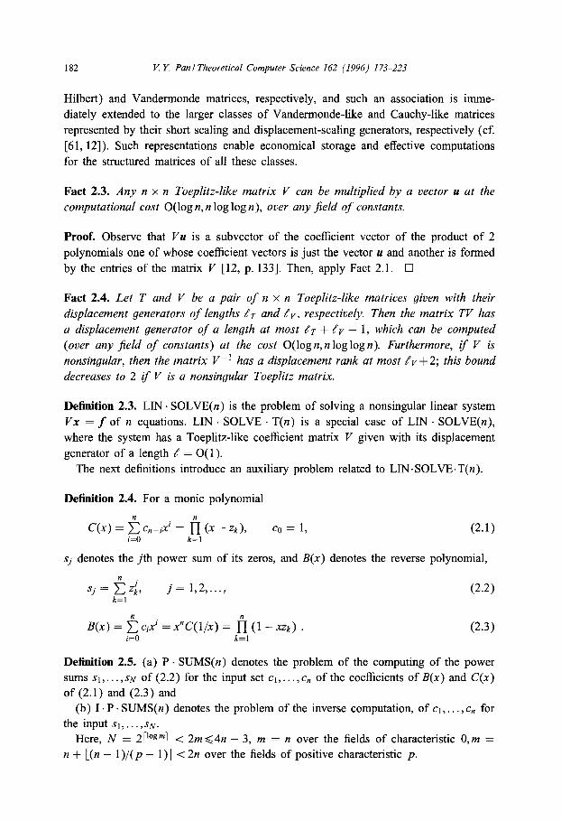
Fact 2.3. Any n x n Toeplitz-like matrix V can be multiplied by a vector u at the computational cost O(log n, n log log n), over any field of constants.

Proof. Observe that Vu is a subvector of the coefficient vector of the product of 2

polynomials one of whose coefficient vectors is just the vector IC and another is formed

by the entries of the matrix V [12, p. 1331. Then, apply Fact 2.1. 0

Fact 2.4. Let T and V be a pair of n x n Toeplitz-like matrices given with their displacement generators of lengths dr and 8 v, respectively. Then the matrix TV has

a displacement generator of a length at most 8~ + ev + 1, which can be computed (over any field of constants) at the cost O(logn,n log log n). Furthermore, tf V is

nonsingular, then the matrix V-’ has a displacement rank at most er +2; this bound decreases to 2 tf V is a nonsingular Toeplitz matrix.

Definition 2.3. LIN . SOLVE(n) is the problem of solving a nonsingular linear system

Vx = f of n equations. LlbI . SOLVE . T(n) is a special case of LIN . SOLVE(n),

where the system has a Toeplitz-like coefficient matrix V given with its displacement

generator of a length / = 0( 1).

The next definitions introduce an auxiliary problem related to LIN.SOLVE.T(n).

Definition 2.4. For a manic polynomial

n n C(X) = C C,_i.2 = n (X - Zk), CO = 1, (2.1)

i=O k=l

Sj denotes the jth power sum of its zeros, and B(x) denotes the reverse polynomial,

k=l

j= 1,2,..., (2.2)

B(X) = eCiXi =x”C(l/‘~) = fi (1 -XZk) .

i=O k=l (2.3)

Definition 2.5. (a) P . SUMS(n) denotes the problem of the computing of the power

sums si,. . .,sN of (2.2) for the input set cl,. . ., c, of the coefficients of B(x) and C(x)

of (2.1) and (2.3) and

(b) 1. P. SUMS(n) denotes the problem of the inverse computation, of cl,. . . , c, for

the input si, . . . , sN.

Here, N = 2r“‘aml < 2m<4n - 3, m = n over the fields of characteristic 0,m = n + [(n - 1 )/(p - 1 )] < 2n over the fields of positive characteristic p.


The solution of P . SUMS(n) may rely on Newton’s identities,

k-l

Sk + C ciSk__i f kCk = 0, k = l,...,n, (2.4) i=l

Sk $ 5 cisk_i = 0, k=n+l,...,N. (2.5) i=l

These identities form a triangular Toeplitz linear system of N equations in sr,sz, . . ,sN;

such a system can be solved (over any field of constants) [12] at the cost bounded by

O((logn) log* n, (n log log n)/ log* n), since N < 4n. In this paper we actually care only about 1. P. SUMS(n) because of the next result.

Fact 2.5. LIN . SOLVE. T(n) for a linear system Vx = f can be reduced (over any field of constants) to I. P. SUMS(n) for C(x) equal to the characteristic polynomial

of VW, for any fixed nonsingular Toeplitz-like matrix W; the arithmetic cost of this

reduction is bounded by O((log n)*, (n* log log n)/ log n).

Proof. Fact 2.5 for W = I is supported by the main algorithm of [63]. The extension

to any nonsingular Toeplitz-like matrix W follows from Facts 2.3 and 2.4 since one

may first solve the linear system (W)y = f and then compute the vector x = Wy, satisfying Vx =f: 0

The main algorithm of [63] and its analysis in [63] relying on Fact 2.5 have consti-

tuted a major step towards the solution of the problem LIN. SOLVE. T(n). It remained

to solve the problem I.P.SUMS(n), and we will do this in Sections 3-5. In these sec-

tions, we will rely on Newton’s identities of (2.4), (2.5) rewritten in a more compact

form, as the polynomial identity

XB’(X) = -B(X)2 SiXi, (2.6)

i=l

which can be obtained from the next simple basic identity,

X@(X)/&) = -&k,(l - xzk). k=l

Definition 2.6. The n x n matrix

F = F(c) =

(having its first superdiagonal filled with ones, its last row with the vector c =

(c,, . .,cl), and all the other entries with zeros) is called the Frobenius (companion)

184 V. Y. Pant Theoretical Computer Science I62 (1996) 173-223

matrix of the polynomial C(x) of (2.1). For a square matrix T, we write CT(X) =

det(xZ - T) to denote the characteristic polynomial of T.

Fact 2.6. c&X) = det(xI - F), the characteristic polynomial of F = F(c), has the coefficient vector c and, therefore, coincides with C(x) of (2.1).

Fact 2.7. The matrix F has a displacement generator (X, Y),

( 1 0 0 0

0 1 0 . ..oo

XT= . . . =

0 0 . . . 0 1 >

’ yT

(

3 &I C,-1 c,4 . . . c2 Cl )

of a length at most 2.

In Section 5, we will use randomization based on the following well-known fact,

due to [29] (compare also [85,80, 12, Lemma 1.5.1, p. 431).

Fact 2.8. Let P(x) = P(xI,x~ , . . . ,x,,,) be a nonzero m-variate polynomial of a total degree d. Let S be a finite subset in the given field of constants or in its fixed

extension field and let X* = {x:, . . . ,xE} be a point in S”, where all xi are chosen at random in S, independently of each other, under the untform probability distribution on S. Then Probability {P(X*) = O}<d/lSI, h w ere ISI denotes the cardinality of

S.

Definition 2.7. Hereafter, S will denote a fixed (and sufficiently large) finite set, and

all random values will be chosen from S independently of each other and under the

uniform probability distribution on S. Our randomized estimates for computational cost

will not include the cost of generation of such random parameters. ISI will denote the

cardinality of S.

The next definition is important for our algorithm of Section 5 and is also used in

Section 12.

Definition 2.8 (Brent et al. [17]; Bini and Pan [12]). For two nonnegative integers k

and h and for a formal power series Q(x) = CrOqixi or, as an equivalent alternative,

for a fixed N > k + h and for a polynomial Q&x) = CEoqixi, the (k, h) entry of the

Pad& approximation table (hereafter referred to as the Pad& table) is defined as a pair

of polynomials U(x) and V(x) # 0 of degrees at most k and h, respectively, such that

U(x) - Q(x)V(x) = Omodx k+h+l. This entry degenerates if U(x) and V(x) have a

nonconstant common divisor or if deg U(x) < k and deg V(x) < h.

Fact 2.9 (Gragg) (cf. [17, Theorem 21). Suppose that the polynomials U(x) and V(x) of Definition 2.8 are relatively prime, that is, have no nonconstant common divisors. Then we have the 2 simultaneous bounds, k > deg U(x) and h > deg V(x), tf and only tf the associated h x h Toeplitz matrix Q = (qi,j) is singular, where

V. Y Pan1 Theoretical Computer Science 162 (1996) 173-223 185

qij = qk__i+j, i, j = 0, 1,. . ., h - 1, qe = 0 for e < 0. Furthermore, r = rank Q =

h - min(k - deg U(X), h - deg V(X)).

Corollary 2.1. Under the assumptions of Fact 2.9, the Y x r southeastern submatrix

of the matrix Q is nonsingular.

Fact 2.10. The computation of the (k, h) entry of the Pad& table for 2 given nonnegative integers k and h and for a formal power series Q(x) = Czoqix’ can be reduced to computing the rank r of an h x h Toeplitz matrix, solving a nonsingular Toeplitz linear system of r equations, and multiplication of a k x k triangular Toeplitz matrix

by a vector. Furthermore, the rank computation can be omitted tf it is known that

the (k, h) entry of the Pad& table does not degenerate.

Fact 2.10 is supported by Algorithm 2.5.1 from p. 140 of [12], which relies on the

proof of Theorem 1 of [17] and on our Fact 2.9 and Corollary 2.1.

Definition 2.9. The (m + n) x (m + n) matrix R = [U, V], whose 2 blocks U and

V are the (m + n) x m and (m + n) x n Toeplitz matrices, respectively, defined by

their first rows [u,, 0,. . . , 0] and [v,, 0,. . . ,O], respectively, and by their first columns

[u,, u,_l,. . . , uo,O,. . . , OIT and [v,, v,-1,. . . , vo,O,. . . , OIT, respectively, is called the

Sylvester or resultant matrix, associated with the polynomials u(x) = Cy=ouix’ and

v(x) = ~~=,vix’. The (m + n - 2k) x (m + n - 2k) submatrix Rk = [uk, vk] ob-

tained by deleting the last 2k rows of R, U, and V and the last k columns of each

of U and V is called the kth subresultant matrix, for k = 0, 1, . . , min{m, n}. (In

particular, Ro = R.) detR is called the resultant of the 2 polynomials U(X) and

v(x).

By inspection, we immediately deduce the next result.

Fact 2.11. The kth subresultant matrix Rk has a displacement generator of length 2> given by the (m + n - 2k) x 2 matrices

T X(k) = ‘,I . . . U2k--m+l

%I - t&,+,-k UZk-nil - Ukfl

and y&f = [e(0),eW+l)], . .

where uk = vk = 0 tf k < 0, uj = 0 tf j > n, and the vector ech) has its hth coordinate equal to 1 and other coordinates equal to 0.

Fact 2.12. Under DeJinition 2.9, u(x) and v(x) have a nonconstant common divisor andlor u, = v, = 0 tf and only tf det R = 0.

Corollary 2.2. Under Definitions 2.8 and 2.9, the (k, h) entry of Pad6 table degenerates tf and only tf the associated resultant vanishes, that is, det R = det R( U, V) = 0, for U(x) and V(x) considered as polynomials of degrees k and h, respectively.

186 V. Y. PanITheoretical Computer Science 162 (1996) 173-223

3. From power sums to coefficients over the fields

of characteristic 0 or greater than n

In this section we will solve the problem I . P . SUMS (n) over the fields of con-

stants that have characteristics p = 0 or p > n. In this case, the block substitution

algorithm reduces the solution of the system (2.4) to multiplication of an Ln/2j x [n/2]

Toeplitz matrix by a vector and to solving a pair of structured linear systems, similar

to (2.4) but of half-size [12]. By recursively applying block substitution to the two

latter systems and by using Fact 2.3, we may compute cl,. . . , c,, at the overall cost

O(n log n, (log n) log log n).

Actually, we will apply another algorithm, running faster (see Theorem 3.1 at the

end of this section). We have extracted the construction of this algorithm from the

proof of Lemma 13.1 on p.40 of [78], where it was assumed that the input polynomial

had all its zeros in the unit disc {x: 1x1 < 1) and where the presentation was directed

towards estimating the bit-complexity of the solution.

The algorithm is iterative and exploits Eq. (2.6). The input is formed by the power

sums of the zeros of B(x), and the coefficients CO and cl of B(x) are readily available.

Each recursive step of the algorithm doubles the number of the available coefficients.

Let us specify this algorithm. Write

Hk(x) = B(x)modXk+’ = 5 cixi, (3.1) i=O

observe that Hi(x) = 1 - SIX is available, and recursively compute the coefficients of

ffZ(X),ff4(X), . . . ,ff2dX), v = [logn], by using the equations

ff2k(X) = ffk(X)&(X)modX 2k+l

, (3.2)

where &(x) are unknown auxiliary polynomials, and we easily deduce from (3.2) that

2k k-l

j Rk(X) = C rk,jX = 1 +Xk+’ C ?“k,k+i+l.X?y (3.3) j=O i=O

k = 1,2,4 ,..., 2”-‘. From (3.1)-(3.3), it is straightforward to deduce that

R;(x) = ($&)/&(x))modx 2kfl

>

ff;k(X)/ff2k(X) = (H;(X)Rk(X) + ffk(X)#&X))/(Hk(X)Rk(X))

= (f$(X)/Hk(X)) + R;(x) modx 2k+l .

By combining the latter equation with (2.6), we obtain that

2k+l - R;(X) = ffi(X)/ffk(X) + c SiXi-’ modx2k+1.

i=l (3.4)

Given si ,...,Slk+i and&(x) =B(x)modxkfl, we apply (3.4) in order to compute

the coefficients of the polynomial R:(x) = xfLol(k+i+ l)rk,k+i+i~?+~ [cf. (3.3)]. Then,

Y Y. Panl Theoretical Computer Science 162 (1996) 173-223 187

we immediately recover the coefficients YQ+~+~ of I&(X), for k + i + 1 <n. (Under this

bound, k + i + 1 # 0 mod p for p > n, so that k + i + 1 has reciprocal in any field of

characteristic 0 or greater than n.) Finally, we compute I&(x) by using (3.2).

The entire computation amounts to computing polynomial sums and products, as

well as the reciprocals of polynomials with x-free terms equal to 1. More precisely, at

the kth recursive step, we perform 0( 1) such operations modulo x2k +‘. We may imple-

ment them either at the cost O((log k) log* k, (k log log k)/ log* k) or, at our alternative

choice, at the cost O(log k, (log log k)2k) for k = 1,2,4,8.. . , [lognl - 1 (compare

facts 2.1 and 2.2). By using Brent’s principle, we slow down O(loglogk) initial steps

slightly, so as to be able to use fewer processors, and arrive at the following result.

Theorem 3.1. The problem I. P.SUMS (n) of Definition 2.5 can be solved over any

field F of characteristic p = 0 or p > n at the cost bounded by O((logn)*, (loglogn)’

n/ log n) or, alternatively, by O((log n)2 log* n, (n log log n)/((log n) log* n)). More yen-

erally, the latter cost bound applies to the problem of the evaluation (over such a

field F) of the first n coejficients of any formal power series B(x) satisfyiny Eq. (2.6)

modulo x2”+’ and B(0) = 1, where SI , . . . , s2,,+l are the input values.

4. Extension to the computation over any field

By extending the algorithm of the previous section to the computation over any

field of constants that has a characteristic p > 0, we may immediately compute at first

the coefficients of R;(x) and then the coefficients rk,k+i+l of &(x), except for ones

where p divides k + i + 1, since (rk,SPxSP)’ = Omod p for any integer s. Thus, for

0 < p dn, we need to extend the algorithm further in order to compute B(x). Taking

point of view of [47] and [48], we observe that the linear system of Eqs. (2.4) has

a matrix of rank n - [n/p], and we need Ln/pj additional equations from (2.5) in

order to obtain a nonsingular system. By associating the kth equation of (2.4) with the

power sum Sk, we may state the equivalent problem of finding a set K of n positive

integers, K = {kl , . . . , k,}, such that all the coefficients of the polynomial B(x) can be

rationally expressed through the Set Sk,, . . . ,sk,, called a fundamental set of the power

sums.

Schiinhage in [79] has shown (citing [83,41,42,56] as the preceding works) that the

desired properties hold already for the set K of the first n positive integers not divisible

by p. Then, based on this result, he has devised a parallel algorithm for the computation

of the coefficients of the characteristic polynomial of a given general matrix over any

field of constants. Of the 2 possible ways to devising such an algorithm, which both

start with a given fundamental set of power sums of its zeros, he has chosen a way

based (like in the preceding work [47]) on the reduction of the problem to solving a

nonsingular linear system of [n/p] equations. This way has lead him to an algorithm

supporting estimates for the arithmetic parallel complexity of the solution that were

strongly inferior to ones based on the preceding algorithms of [6] and [22].

188 K Y. Pan1 Theoretical Computer Science 162 (1996) 173-223

In this section, we will recall his techniques, though with more complete elaboration

of the transition to the auxiliary power series A(x); moreover, we will introduce ran-

domization and will obtain improved estimates for parallel arithmetic complexity (see

Theorem 4.1, Fact 4.1, and Corollary 4.1). In the next section, we will demonstrate a

further crucial improvement, due to using an alternative approach, based on computing

a PadC approximation of A(x). To make this alternative approach work, we will re-

late it to the associated Frobenius (companion) matrix and to some other Toeplitz-like

matrices and then will define a recursive process of computing PadC approximation by

exploiting the results of Section 2 and some new techniques of regularization of PadC

approximation via randomization. This will lead us to parallel algorithms supporting

the desired (improved) estimates for parallel arithmetic complexity. (Our presentation

in these two sections have some similarity with the presentation in the paper [67], par-

tially reproduced on pp. 373-377 of [12], where similar techniques have been studied

for computations with general matrices.)

We first rewrite B(X) as follows:

p-1 B(x) = c Bk(XPjxk,

k=O (4.1)

where

dk Bk(y) = c ck+ip$, k=O,l,..., p-l, (4.2)

i=O

do=d= 14PJ, dk >dk+l ad - 1, k=O,l,..., p-2. (4.3)

Then we observe that Bo(0) = B(0) = 1 and define p - 1 rational functions,

Akb> = Bkb)/BObh k = l,...,p- 1 (4.4)

as well as the next rational function, which we also represent as a formal power series:

A(X) = B(X)/B()(XP) = C UjX'. i=O

Combining (4.1), (4.2), (4.4), and (4.5), we obtain that

P-1 A(x) = 1 + c xkx&(XP),

(4.5)

(4.6) k=l

which implies that

ao=l, a,=o, s = 1,2,...,

ak = Ck, fork= 1,2 ,..., p- 1.

(4.7)

(4.8)

(4.5) and (4.6) also imply representation of A&) as formal power series for all k.

Now recall (4.2) for k = 0 and observe that Bh(xP) = Omod p. Therefore, (4.5)

implies that A’(x) = B’(x)/&(xP), xA’(x)/A(x) = xB’(x)/B(x).

K Y PanITheoretical Computer Science 162 (1996) 173-223 189

Combine the latter equation with (2.6) and obtain that

.x/i’(x) = -A(x)E SkXk. k=l

(4.9)

We will now prove the following result.

Theorem 4.1. Given the power sums Sk of the zeros of a polynomial C(x), k =

1,2,. . . ,2n [see (2.1), (2.2)], one may compute (ouer any field of constants of a

positive characteristic p) the coeficients al,a2,. . . ,a,,,, m = n+ [(n- l)/(p- 1)J < 2n, of the formal power series A(x) satisfying (4.5), (4.7) uor B(x) of (2.3) and Bo(xP)

of (4.1)] at the parallel arithmetic cost bounded by O((logn)‘, (n(log logn)2)/ log n)

or, alternatively, O((log n)2 log* n, (n log log n)/((log* n) log n)), which are the same bounds as in Theorem 3.1.

Proof. The computation starts with evaluating ai = ci for i < p [see (4.8)], by means

of the algorithm of the previous section. Then we set up = 0, k = p, and again

apply the algorithm of the previous section, this time, however, replacing ci by a, in (3.1), B(x) by A(x) and B’(x) by A’(x) throughout, so that, in particular, (2.6) is

replaced by (4.9), and &(x) is set to equal cfl,aix’. The resulting algorithm works

as before, except that rP,zP cannot be recovered from R’,(x) but is now computed from

the equations

(4.11)

implied by (3.2) and (3.3) for k = p. Substituting (4.7), we deduce that

P--l

r,,2, = - C Wp,2p-i. i=l

Then we immediately compute rp,zp. The same process is recursively repeated for

k = 2p,4p,Sp ,..., until all the ai, i = 1,2,. . . , m, have been computed. Each recursive

step begins with the computation of the coefficients rk# of Rk(x) for k = qp, s =

q+ I,..., 29. This computation relies on the equations

sp-1

- ,s airqp,sp-i = asp, s = 4+ L...,%

which extend (4.11) from the case s = 2, q = 1. Substitute (4.7) and obtain the

equations

SP-I

r,,,, = - zs air9P,~P-i~ s=q+ 1,...,2q.

NOW replace rqp,sP_i by r$,Sp_i on the right-hand sides, where r$Sp_i = 0 if p divides *

1, rqJ’,sp-i = rgp,sp-i otherwise. Since ai = 0 if p divides i and if i > 0, the right-hand

190 V. Y. PanITheoretical Computer Science I62 (1996) 173-223

sides do not change and, therefore,

sp-1

rqp,sp = - c W~p,sp-_iy s = q+ 1,...,2q. i=l

(4.12)

Here, ai and rfp,sP_i are known for all i, and we obtain all the rqp,sp from (4.12) as

the coefficients of a polynomial product, at the cost O(log q, q log log q), (cf. Fact 2.1).

Having computed the rqp,sp for all s, we then recall (3.2) and obtain the coeffi-

cients aqp+l, . . . , azqp of Hzqp(x), at the cost within the same bound, due to Fact 2.1.

This completes the recursive step of computing the coefficients ak+l, ak+& . . . , a2k for

k = qp. The computational cost of this step is bounded according to the estimates of

Section 3 for the cost of the transition from Hk(X) to i&(X) for k = qp. Therefore, in

[log n] + 2 recursive steps, we compute al,. . . , azn at the cost bounded as we claimed

in Theorem 4.1. 0

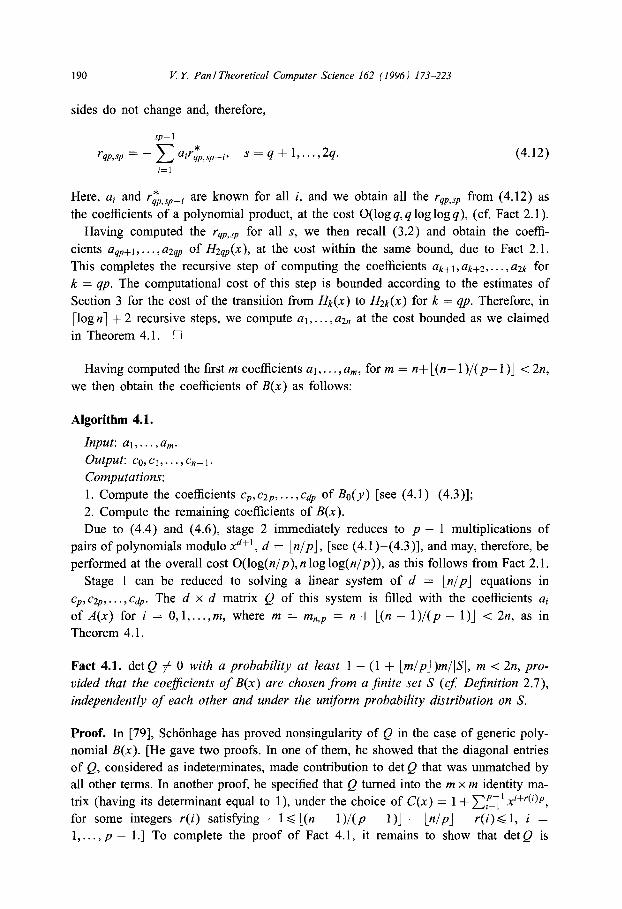
Having computed the first m coefficients al,. . . , a,,,, for m = n+ [(n- 1 )/(p- 1 )I < 2n, we then obtain the coefficients of B(x) as follows:

Algorithm 4.1.

Input: al,...,a,. Output: CO,CI,. . .) C,_].

Computations: 1. Compute the coefficients cp, czP, . . . , Cdp of B&) [see (4.1)-(4.3)];

2. Compute the remaining coefficients of B(x).

Due to (4.4) and (4.6), stage 2 immediately reduces to p - 1 multiplications of

pairs of polynomials modulo xd+‘, d = [n/pj, [see (4.1)-(4.3)], and may, therefore, be

performed at the overall cost O(log(n/p), 12 log log(n/p)), as this follows from Fact 2.1.

Stage 1 can be reduced to solving a linear system of d = [n/p] equations in

cp, c2p, . . ..cdp. The d x d matrix Q of this system is filled with the coefficients ai

of A(x) for i = O,l,...,m, where m = mn,p = n + [(n - l)/(p - l)] < 2n, as in

Theorem 4.1.

Fact 4.1. det Q # 0 with a probability at least 1 - (1 + lrn/p] )m/lSI, m < 2n, provided that the coeflcients of B(x) are chosen from a jinite set S (cf Dejnition 2.7),

independently of each other and under the uniform probability distribution on S.

Proof. In [79], Schijnhage has proved nonsingularity of Q in the case of generic poly-

nomial B(x). [He gave two proofs. In one of them, he showed that the diagonal entries

of Q, considered as indeterminates, made contribution to det Q that was unmatched by

all other terms. In another proof, he specified that Q turned into the m x m identity ma-

trix (having its determinant equal to l), under the choice of C(x) = 1 + C[=y’ x~+~@)P,

for some integers r(i) satisfying - 1 < [(n - 1 )/(p - I)] - [n/p] - r(i) G 1, i = 1 ,..., p - 1.1 To complete the proof of Fact 4.1, it remains to show that det Q is


a polynomial of a degree at most (1 + lm/~] )m in the coefficients cl, ~2,. . , c, of C(x)

and B(x) (and then, Fact 4.1 will follow from Fact 2.8). Let us do this.

Recall (4.5) and obtain that A(x) mod xm+’ = B(x) cr,( 1 - &(xP))’ mod x”+’ Since xp divides 1 - Ba(xJ’), we have (1 - &,(xJ’))’ mod x”+’ = 0 for i > m/p. There-

fore, the coefficients UI,U~, . . . ,a, of A(x) mod xm+’ are polynomials in ci,cl,. , c, of

degrees at most 1 + Lrn/~]. Since Q is an m x m matrix, det Q is a polynomial in

CI,C2,...,Cn of a degree at most (1 + Lm/p] )m. C

Let us now assume that the coefficients cl, ~2,. . . , c, of C(x) and B(x) have been

randomly chosen (from a fixed finite set S of Definition 2.7) but remain unknown,

whereas the power sums s1 ,sz,. ,s, are known. Such an assumption can be implicitly

motivated by Fact 4.1, but our actual motivation is more direct. It relies on the reduction

of our main problem LIN.SOLVE.T(n) for an arbitrary nonsingular Toeplitz-like input

matrix V to the same problem but for a random Toeplitz-like input matrix VW and,

consequently, to the associated problem I P SUMS(n), corresponding to a random

characteristic polynomial C(x). We will exploit such a reduction in the next section.

By summarizing our analysis of stages (a) and (b) of Algorithm 4.1, we arrive at

the following result.

Corollary 4.1. For a pair of natural n and p, for m = nt L(n - l)/(p- l)] < 2n, and

for u given set of the values s1 ,SZ, ,s, of the power sums of the zeros of u random

polynomial C(x) of (3.1), with its unknown coefficients (chosen from a fixed set S

of a cardinality IS/, independently of each other and under the uniform probubility

dist.ribution on S), the problem I. P . SUkfS(n) of Definition 2.5 can be solved

(over any field of constants of a positive characteristic p), with a probability at least

1 -( 1+ Lm/p] )m/lSl, at the asymptotic cost bounded by the cost bound of Theorem 4.1

augmented by the complexity of solving the problem LIN . SOL VE( [n/p] ).

5. Improved algorithms and complexity bounds

In this section, some new techniques will enable us to extend Corollary 4.1 by

devising a randomized algorithm for the problem LIN . SOLVE . T(n) over any field

of constants of a characteristic p > 0. Moreover, we will simplify the computation of

the coefficients of &(y) and will arrive at the improved complexity estimates.

Due to (4.4) the coefficients cp, c+ . , cdp of&(y) can be obtained from the (dl, d)

entry of the Padt approximation table for the power series At(y) (compare Defini-

tion 2.8), where At(y) = Ai is defined by A(x), due to (4.5) and (4.6) and

dl <d = ln/pJ, due to (4.3). Unless degeneration occurs, that is, unless c, = c,_l = 0

and/or B,(y) and Be(y) have a nonconstant common divisor, such a (dl,d) entry of

the table is filled with the pair (Bl(y),Bo(y)) and can be computed by means of the

known reduction of the problem to solving a nonsingular Toeplitz linear system of d

equations (see Fact 2.10).

192 K Y. Panl Theoretical Computer Science 162 (1996) 173-223

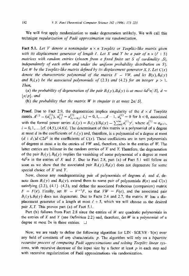
We will first apply randomization to make degeneration unlikely. We will call this

technique regularization of Padt? approximation via randomization.

Fact 5.1. Let V denote a nonsingular n x n Toeplitz or Toeplitz-like matrix given with its displacement generator of length e. Let X and Y be a pair of n x (8 f 5)

matrices with random entries (chosen from a fixed finite set S of cardinality jS(, independently of each other and under the urnform probability distribution on S).

Let W be the Toeplitz-like matrix defined by its displacement generator X, Y. Let C(x)

denote the characteristic polynomial of the matrix F = VW, and let B(x),Bo(y) and B,(y) be the associated polynomials of (2.3) and (4.2) for an integer p > 1.

Then, (a) the probability of degeneration of the pair Bl(y),Bo(y) is at most 4d*n/lSI, d =

ln/~I, and (b) the probability that the matrix W is singular is at most 2n/lSJ.

Proof. Due to Fact 2.9, the degeneration implies singularity of the d x d Toeplitz

matrix A(‘) = (a&j), a!,\’ = af,)i+j; i,j = 0,l ,...,d - 1, a;) = 0 for h < 0, associated

with the formal power series Al(y) = Bl(y)/Bo(y) = CrOai’)y’, where a!‘) = ab+l,

i = O,l,... [cf. (4.5), (4.6)]. The determinant of this matrix is a polynomial of a degree

at most d in the coefficients of A 1 (y ) and, therefore, is a polynomial of a degree at most

(d + dl )d 62d* in the coefficients of C(x). These coefficients are in turn polynomials

of degrees at most n in the entries of VW and, therefore, also in the entries of W. The

latter entries are bilinear in the random entries of X and Y. Therefore, the degeneration

of the pair Bl(y), Be(y) implies the vanishing of some polynomial of a degree at most

4d*n in the entries of X and Y. Due to Fact 2.8, part (a) of Fact 5.1 will follow as

soon as we show that the associated pair Bl(y), Be(y) does not degenerate for some

special choice of X and Y.

Now, choose any nondegenerating pair of polynomials of degrees dl and d, de-

note them Bl( y) and Be(y), extend them to some pair of polynomials B(x) and C(x)

satisfying (2.3), (4.1)-(4.3), and define the associated Frobenius (companion) matrix

F = F(c). Finally, set W = V-‘F, so that VW = F(c), and the associated pair

B,(y), Be(y) does not degenerate. Due to Facts 2.4 and 2.7, the matrix W has a dis-

placement generator of a length at most 8 + 5, which we will choose as the desired

pair X, Y. This proves part (a) of Fact 5.1.

Part (b) follows from Fact 2.8 since the entries of W are quadratic polynomials in

the entries of X and Y (see Definition 2.2) and, therefore, det W is a polynomial of a

degree at most 2n in these entries. 0

Now, we are ready to define the following algorithm for LIN . SOLVE . T(n) over

any field of constants of any characteristic p. The algorithm will rely on a bipartite recursive process of computing Pad& approximations and solving Toeplitz linear systems, with recursive decrease of the input size by a factor at least p in each step and

with recursive regularization of Pad& approximations via randomization.

V. Y. Panl Theoretical Compuier Science 162 (1996) 173.-223 193

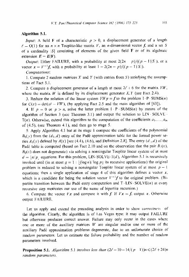
Algorithm 5.1.

Input: A field F of a characteristic p > 0, a displacement generator of a length

e = 0( 1 j for an n x n Toeplitz-like matrix V, an n-dimensional vector L and a set S

of a cardinality ISI consisting of elements of the given field F or of its algebraic

extension E = E(F).

Output: Either FAILURE, with a probability at most 2(2n + p)l((p - 1 )lSl), or a

vector x = V-If; with a probability at least 1 - 2(2n + p)/((p - l)lSl).

Computations:

1. Compute 2 random matrices X and Y (with entries from S) satisfying the assump-

tions of Fact 5.1.

2. Compute a displacement generator of a length at most 2/ + 6 for the matrix VW,

where the matrix W is defined by its displacement generator X, Y (see Fact 2.4).

3. Reduce the solution of the linear system Vwy = f to the problem I . P SUMS(n)

for C(X) = det(x1 - VW), (by applying Fact 2.5 and the main algorithm of [63]).

4. If p = 0 or p > n, solve the latter problem I P SUMS(n) by means of the

algorithm of Section 3 (see Theorem 3.1 j and output the solution to LIN SOLVE

T(n ). Otherwise, extend this algorithm to the computation of the coefficients al, . , a,

of (4.5), (see Theorem 4.1), and then go to stage 5.

5. Apply Algorithm 4.1 but at its stage 1 compute the coefficients of the polynomial

B&j from the (di,d) entry of the Pade approximation table for the formal power se-

ries Al(y) defined by A(x) [see (4.4), (4.6), and Definition 2.81. The entry (cl’, , d) of the

PadC table is computed (based on Fact 2.10 and on the observation that the pair B,(x).

&(x) does not degenerate) via solving a nonsingular Toeplitz linear system of at most

d = Ln/pj equations. For this problem, LIN.SOLVE.T(d), Algorithm 5.1 is recursively

invoked until (in at most g = 1 + L(log n)/ log pj its recursive applications) the original

problem is reduced to solving a nonsingular Toeplitz linear system of at most p - 1

equations; then a single application of stage 4 of this algorithm defines a vector X,

which is a candidate for being the solution vector V-If to the original problem. (Bi-

partite transition between the Pad& entry computation and T. LIN. SOLVE(n) at every

recursive step motivates our use of the name of bipartite recursion.)

6. Compute the vector Vx and compare it with J If Vx = J; output x. Otherwise

output FAILURE.

Let us apply and extend the preceding analysis in order to show correctness of

the algorithm. Clearly, the algorithm is of Las Vegas type: it may output FAILURE

but otherwise produces correct answer. Failure may only occur in the cases where

one or more of the auxiliary matrices W are singular and/or one or more of the

auxiliary Padt approximation problems degenerate, due to an unfortunate choice of

random parameters. Let us estimate the failure probability and the number of random

parameters involved.

Proposition 5.1. Algorithm 5.1 involves less than (2f + 10 + 14/( p - 1 ))n d (2/ + 24)n

random parameters.

194 V. Y Pan1 Theoretical Computer Science 162 (1996) 173-223

Proof. Recall that at most g = 1 + l(logn)/ log pJ random Toeplitz-like matrices

are involved in computations by Algorithm 5.1; furthermore, due to Fact 5.1, their

displacement generators have lengths at most & + 5 at the first recursive step and

at most 7 at all the subsequent steps (since at the latter steps, we deal with Toeplitz

linear systems arising from Pad6 approximation problems and since for such systems we

may replace / by 2 in the estimate of Fact 5.1). Therefore, the displacement generator

is defined by 2(e + 5)n parameters at the 0th recursive step and by 14~ < 14n/pk

parameters at the kth recursive Step, where p 2 2, nk = Lnk_t/pj, no = n, k = 1,2,. . . .

This implies that a total of 2(/ + 5)n + 14 ~~~~ n/, 62(6 + 5)n + l4n ~~~~ ppk <

(2e + 10 + 14/(p - l))n<(2& + 24)n parameters are involved in Algorithm 5.1. 0

Proposition 5.2. Algorithm 5.1 outputs either FAILURE, with a probability at most

(2np/lSl)(l/(p - 1) + 2n2/(p3 - l)), or the correct solution.

Proof. We recall that Algorithm 5.1 fails only if, for some k, at the kth recursive

step of its computation, the auxiliary matrix W is singular and/or the associated Pad&

approximation problem degenerates. Due to Fact 5.1, such 2 events may occur with

probabilities bounded by 2nk/]S( and 4ni/(p21S/), respectively. Therefore, while we

perform Algorithm 5.1, we will encounter no singularity with a probability at least

and will encounter no degeneracy with a probability at least

Therefore, Algorithm 5.1 outputs the correct solution with a probability at least

( l- 2nP (P- l)lSl x l-

4n3p

(p3 - l)]Sl ’ 1 - >

2nP 4n3p

(P - l)lSl - (P3 - l)lSl

=l-?!Y l ( 2

-~ JSI P-lt(pk) . 1

It follows that the failure probability is at most (2np/JSI)( l/(p - 1) + 2n2/(p3 - 1)).

0

This completes the correctness proof for Algorithm 5.1, and Proposition 5.1 bounds

the number of random parameters involved in this algorithm.

By using our analysis in this and previous sections (in particular, cf. Fact 2.10),

we easily estimate the computational cost of performing Algorithm 5.1, in the case

where IS] d IFI [see (5.3) below]. We also need to consider the opposite case, where

)S) > IFI. Indeed, due to Proposition 5.2, it suffices to choose

IS( = 28A, il = n(n, p) = 2np (

5 + & , >

(5.1)


in order to bound the probability of failure of Algorithm 5.1 by 2_fr, for any fixed p.

The value IS/ of (5.1), however, may exceed the cardinality IFI of the field F of

constants (where (FI > p but can indeed be as small as p). Then, we will choose the

set S in an algebraic extension field E of polynomials over F reduced modulo a fixed

(irreducible) polynomial of degree

D = [(log ISI>/ 1s IFI1 (5.2) (cf. our Remark 5.1). Such an extension field E has a cardinality IEl>/ ISI.

We note that for fl = O(logn), (5.1) implies that log ISI = O(logn),

D = O((logn)/log IFI).

Any (k - 1)-variate polynomial over E can be represented as a k-variate polynomial

over F whose degree in the new variable (defining the extension field E over F) is at most D - 1. On the other hand, inspection of Algorithm 5.1 and of the main

algorithm of [63] (supporting stage 3 of Algorithm 5.1) shows that all their operations

are ultimately reduced to computing polynomial sums, products, and reciprocals modulo

some powers of x. We combine the latter observation with (5.1), (5.2) Remark 2.1,

Propositions 5.1,5.2, and various results involved in the description of Algorithm 5.1,

and arrive at the following theorem.

Theorem 5.1. Let F be a field of a characteristic p, let fl be a positive scalar,

( 1 i=2np ~

p-l +(pJ-l) x)<4n(l+T) for p32

[cf. (5.1)], N = 2fl1, D = [(logN)/log IFI], and S be a jixed finite set of cardinality

ISI == N and with elements either from the field F if F has a cardinality IFI at least

N or from a jield E being an algebraic extension of F of degree D. Then, Algo-

rithm 5.1 solves the problem LIN. SOLVE. T(n) at a deterministic cost bounded by

C, := 0((logn)2,(n210glogn)/logn), if p = 0 or p > n [cf. (1.2)]. Zf 0 < pdn,

Algorithm 5.1 solves the same computational problem at a randomized cost bounded

by

GP = O((log nj2y(n, PI, (n2 log 1% n)lMn, P) 1% n)> for IFI 2N (5.3)

and by

C n,p,F = O((log n12y(n, P>, (n2 1% 1% n)(lWWy(n, p)(l% n) 1% IFI 1) for (Fj < N

[which turns into

(5.4)

C n,p,F = 0((lwn)2y(n, p), (n2 1s 1s n)l(y(n, p> loi3 IFI 1) if P = Wx n>l,

where

y(n, PI = r(log n>l 1% Pl. (5.5)

196 K Y. Pan I Theoretical Computer Science 162 (1996) 173-223

In the cases where O<pdn, the computation involves at most (2e+10+14/(p- l))n<

(26 + 24)n random parameters Cfor p >2), chosen from the set S, independently of

each other and under the untform probability distribution on S, where & denotes the length of the displacement generator that defines the Toeplitz-like input matrix. Furthermore, in the case where 0 < p <n, the output is either FAILURE with a

probability at most (2np/N)( l/(p - 1) + 2n2/(p3 - 1)) <2-p or a correct solution, whose correctness test has a cost O(logn,n log log n). The randomized cost estimates

include neither the cost of computing the polynomial E(x) that defines the algebraic extension field E (see Remark 5.1 below) nor the cost of generating random

parameters.

Remark 5.1. In Theorem 5.1 and similarly in the theorems of the next sections, the

degree D of the auxiliary algebraic extension field is defined by (5.2) and is O(B +

logn). If /? = O(logn) and F = F, is a finite field with p elements, then the algorithm

of [81] computes a basic irreducible polynomial defining an algebraic extension field of

degree D over F at the cost O((logn)log(np), I), which for us turns into O((logn)2, 1)

since p dn in applications in this paper.

Remark 5.2. In Algorithm 5.1, we may modify stages 2 and 3, so as to choose

random matrices X and YT of size n x (8 + 2) and a random n x n Frobenius

matrix F of Definition 2.6, at stage 2, and to replace VW by VWF, at stage 3.

Then, only (2L+ 19)n random parameters are needed in the algorithm, but our up-

per bounds on the probability of encountering singularity and/or degeneracy increase

a little, so as to reach (2np + l)/[(p - l)]Sl] and 6n3p/[(p3 - l)]Sl], respectively.

Similar modifications of randomization are possible in the algorithms of the next sec-

tions.

Remark 5.3. Algorithm 5.1 for W = I can serve as a heuristic algorithm for I . P .

SUMS(n), which may only fail in the case of degeneracy of a Pad& approximation

computed at stage 5 (also cf. Remark 7.3 in Section 7).

Remark 5.4. The precise estimates for the number of random parameters and

for the failure probability in Theorem 5.1 and in the theorems of the next sections are

quite complicated. The reader, however, may greatly simplify these estimates by writing

them in a less specific form as follows: choosing no(l) random parameters from a set S

of a cardinality /SI = no(‘) suffices in order to ensure simultaneously the potential work

bound 0((n2 log log n)(log n)2/ log min{ IF], n}), the time bound O((log n)g(y(n, P)~)), and the upper bound 2-p for any positive p = O(logn) on the failure

probability, where IFI is the cardinality of the given field of constants, 26963,

O<h<2, and y(n,p) is defined by (5.5). The estimates in this form are easier to

comprehend, in many cases they are sufficient, and their derivation is less

tedious.

V. Y. Pan I Theoretical Cbmputer Science 162 (1996) 173-223 197

6. Extension to computation of the inverses and the determinants

of Toeplitz-like matrices

Let an n x n Toeplitz-like matrix V be given with its short displacement generator

of a length P = 0( 1). Then the algorithms of [63] enable us to compute (over a field

of constants of a characteristic p) the characteristic polynomial Cv(x), the determinant

det V, and if det V # 0 (that is, if V is nonsingular), then also V-‘, at the overall

deterministic cost C,, of (1.2), provided that p = 0 or p > rt.

Now, let 0 < pdn. Further inspection of Algorithm 5.1 immediately enables us to

extend the estimates of Theorem 5.1 to the problem of the computation (over any

field F) of the coefficients of the characteristic polynomials C,,(X) and C,(x) of

II x n matrices VW and V, where V and W are n x II Toeplitz-like matrices, V is

nonsingular, a displacement generator of length / for V is given as a part of the input,

and a displacement generator of length ( + 5 is randomly chosen for W. The x-free

terms of CVW(X) and CW(X) are equal to (-1)” det( VW) = (-1 )“(det l’) det W and

(- 1)” det W, respectively. With a probability at least 1 - nilSI, we have det W # 0

(due to Fact 2.8) and then we obtain

det V = CVW(O)/CW(O).

The computational cost bounds of Theorem 5.1 apply here too (though with the double

number of random parameters and the double failure probability since we apply The-

orem 5.1 twice, to IQ’ and V). Furthermore, given a nonsingular IZ x n Toeplitz-like

matrix T and its characteristic polynomial CT(x), we may apply an algorithm from [63]

(also available in [12]) in order to compute the matrix T-’ at the cost bounded by C,

of (1.2). By applying this result to T = VW, we obtain (VW))’ and V-’ = W( VW)-’

at the overall randomized cost bounded according to Theorem 5.1.

The presented randomization is of Monte Carlo type. To yield Las Vegas random-

ization for VP’, we multiply, at the cost O(log n,n2 log logn), the computed matrix

V-’ by the input matrix V. If the product gives us the identity matrix, then the matrix

VP’ has been computed correctly, and we output it. Otherwise, we output FAILURE.

Clearly, the algorithm always outputs FAlLURE if V is singular, and our randomized

computation of V-’ is of Las Vegas type, indeed. On the other hand, we recall that

randomization was only needed in the transition from the power sums si to a character-

istic polynomial. Therefore, we may alternatively verify correctness of the output matrix

VP’ (as well as of the output value det V) by testing correctness of such transitions to

the characteristic polynomials CVW(X) and Cw(x). The latter tests are reduced to solving

triangular Toeplitz linear systems of Newton’s identities in the power sums si [cf. (2.4)

(2.5)], which can be done at the cost O((logn) log* n,(nloglogn)/log* n) [l 11.

Furthermore, the same correctness tests can be applied to certify nonsingularity of V.

[V is certified to be nonsingular unless FAILURE is output. In the latter case, we may

conclude (with a low error probability) that V is singular.] Thus, we may relax the as-

sumption about nonsingularity of V and arrive at the following result (cf. Remark 5.4).

198 K Y. PanITheoretical Computer Science 162 (1996) 173-223

Theorem 6.1. The estimates of Theorem 5.1 apply to the parallel arithmetic com-

plexity of computing det V (with double number of random parameters and double failure probability) and V-’ for an n x n Toeplitz-like matrix V. Over the fields of characteristics p = 0 and p > n, the estimates are deterministic. Over the fields of

positive characteristics pdn, the estimates are randomized; they are of Monte Carlo type for testing tf V is singular, and they are of Las Vegas type for testing tf V is

nonsingular. If V is nonsingular, they are of Las Vegas type also for computing V-’ and det V.

Remark 6.1. If the inverse of a nonsingular Toeplitz-like matrix V is sought in the

ring of integers modulo ps for a prime p, then one may first compute V-’ mod p,

performing all the field operations modulo p (with a lower precision), and then lift the

solution to V-’ mod pS by means of the algorithm of [MC79], which only involves

matrix multiplications and subtractions. Moreover, as this was pointed out in [64] (cf.

also Algorithm 2.1 of [63] for A = p), all the auxiliary matrices can be computed in

the algorithm of [MC791 with their short displacement generators, which enables us to

decrease the computational cost dramatically.

Remark 6.2. The algorithms of the next section give us a Las Vegas randomized

singularity test for a Toeplitz-like matrix. An alternative approach is via recursive

triangular factorization of V, which also gives us randomized algorithms for computing

matrix ranks and determinants (cf. [57,58, 12, pp. 99, 100, 212, 323; 701).

7. Computation of the rank and the characteristic polynomial

of a Toeplitz-like matrix

In this section we will extend Algorithm 5.1 to the computation of the rank of

an n x n Toeplitz-like matrix V over any field F of any characteristic p and the

characteristic polynomial of V provided that p = 0 or p > n. We will write RANK(n)

and CHAR. POL(n) to denote these two computational problems.

For p = 0 and for p > n, the main algorithm of [63] computes, at the deterministic

cost bounded by C, of (1.2), the characteristic polynomials Cv of V (thus solving

CHAR. POL(n) for p = 0 and p > n) and C,(x) of the 2n x 2n symmetric Toeplitz-

like matrix fi = ($ L). Recall that, for p = 0, rank fi = 2 rank V = 2n - q, where

x4 is the highest power of x that divides C&X), and output rank V = n - (q/2), thus

solving RANK(n) for p = 0. It remains to solve RANK(n) for p > 0. Our Algorithm 7.1 will give us a solution

for p > n via a randomized reduction to CHAR . POL(n). To solve RANK(n) for

O< p Qn, we will shift from the input matrix V to another n x n Toeplitz-like matrix

W having the same rank and having a characteristic polynomial whose associated ratio

Bi(y)/&(y) [cf. (4.1) and (4.2)] satisfies certain degeneracy restriction (to be specified

in Definition 7.2). The problem of computing the characteristic polynomials of matrices

V. Y Pan I Theoretical Computer Science 162 11996) 173-22-Z 199

W of such a class will be referred to as CHAR.POL*(n). We will show reductions of

RANK(n) to CHAR.POL*(n) (in Algorithm 7.1) and of CHAR.POL*(n) to RANK(d),

d = Ln/p] (in Algorithm 7.2). Based on these reductions, we will define a bipartite

recursive process, which will enable us to reduce the problems to CHAR . POL*(k)

for k < p in [(log n)/ log pl - 1 steps, and then the main algorithm of [63] will give

us the desired solution.

We will start with the following definition and auxiliary results.

Definition 7.1. A matrix A has a rank r if the maximum size of its nonsingular sub-

matrix is r x r.

Fact 7.1. Let A be an n x II matrix having a rank r and let L and UT be two

generic n x n unit lower triangular Toeplitz matrices. Then the i x i leading principal

submatrices of the matrix UAL and the i x i trailing principal submatrices of the

matrix LAU are nonsingular for i = 1,2,. . . , r.

Proof. The proof was given in [49] (and is also available in [12, p. 2061) for the

first statement of Fact 7.1, claiming nonsingularity of the leading principal submatrices

of UAL. Essentially, the same proof also applies to the second statement of Fact 7.1,

claiming nonsingularity of the trailing principal submatrices of LAU. Alternatively, we

may apply the first statement of Fact 7.1 to A, L and U replaced by 2, l and 0,

respectively; write L = JDJ, A = JAJ, U = Jh, for J of Definition 2.1, J’ = I, and

then immediately deduce the second statement of Fact 7.1. 0

Fact 7.2. Let, under the assumptions of Fact 7.1, the 2n - 2 indeterminates-entries

of the matrices L and U be replaced by 2n - 2 random parameters chosen from a

finite set S of a cardinality ISI (independently of each other and under the untform

probability distribution on S). Then,

(a) the r x r trailing principal submatrix of LAU is nonsingular with a probability

at least 1 - 2r/lSl, whereas

(b) all the i x i trailing principal submatrices of LAU for i dr are nonsingular with

a probability at least 1 - (r + l)r/]S].

Proof. Observe that the entries of LAU are quadratic polynomials in the entries of

L and U. Therefore, the determinant of the trailing principal submatrix of LAU is a

polynomial of a degree at most 2i in the entries of L and U. Combine this obser-

vation with Facts 2.8 and 7.1 and obtain Fact 7.2. [To deduce part (b), observe that

n:=,(l - 2i/lSl)3 1 - 2x:=, i/IS1 = 1 - (r + l)r/]SI.] 0

By Definition 7.1, all the i x i submatrices of A are singular for i > r, and due

to this property and Fact 7.2, we may devise a randomized algorithm for computing

r = rankA if we apply binary search for the maximum i for which the i x i trailing

principal submatrix of LAU is nonsingular. Over any field, we may test nonsingularity

200 V. Y. Pan1 Theoretical Computer Science 162 (1996) 173-223

of such submatrices of a k x k Toeplitz-like matrix A by applying our randomized

algorithm supporting Theorem 6.1. This will give us rankA in [lognl such successive

nonsingularity tests, at the price of increasing the time bounds of Theorems 5.1 and 6.1

and decreasing their processor bounds by the same factor [log n1.

In this section, we will achieve the same goal by using Las Vegas randomized

algorithms, with no increase of the time bound for p > n and with its increase by factor

r(n, p) of (5.5) for 2 <p <n. As a by-product, we will also solve CHAR. POL*(n).

The next randomized algorithm reduces RANK(n) to CHAR.POL(n), over any field

F of any positive characteristic p.

Algorithm 7.1. [extension from CHAR. POL(n) to RANK(n)].

Input: a field F having a positive characteristic p and a cardinal@ IFI, a black box

subroutine for CHAR . POL(n), a displacement generator of a length e for an n x n

Toeplitz-like matrix V, and a finite set S of cardinality (S(, consisting of the elements

of the field F or of its fixed algebraic extension field E.

Output: either FAILURE (with a probability bounded by some fixed upper bound)

or Y = rank V.

Computations:

1. Choose (8e + 66)n - 2 random values from the set S; 2n - 2 of them are allocated

for the entries of 2 random unit n x n lower triangular Toeplitz matrices L and UT,

2(2/ + 14)n of them form a pair of n x (2e + 14) random matrices X and YT, and

2(2[ + 18)n form a pair of n x (2L + 18) random matrices X+ and Yz.

2. Compute displacement generators for two matrices: of a length at most / + 4 for

LVU and of a length at most 5e + 39 for the matrix

W = GLVUH, (7.1)

where G - ZGZT = XYT and H - ZHZT = X+ Yz (cf. Definition 2.2).

3. Apply the given subroutine for CHAR . POL(n) in order to compute the charac-

teristic polynomial CW(X) of the matrix W; then compute the maximum q such that

x9 divides C&x) and then the value Y- = n - q.

4. Test whether the r_ x r_ trailing principal submatrix of L VU is nonsingular, by

applying the algorithm of Section 6 that supports Theorem 6.1. If so, output r = v_;

otherwise, output FAILURE.

Remark 7.1. Unlike the singularity test of Theorem 6.1, we have Las Vegas random-

ization in Algorithm 7.1: unless FAILURE is output (with a low probability), the

r- x r- submatrix of L VU is nonsingular, and this enables us to verify that r_ = r.

We will first show correctness of Algorithm 7.1 assuming that the unit lower triangu-

lar Toeplitz matrices L and UT, as well as the matrices X, Y, X+, and Y+, are generic

matrices, filled with (8e + 66)n - 2 indeterminates, rather than with (8/ + 66)n - 2

random elements from S. In this case, clearly, we have r = rank V = rank W, for W

of (7.1), and furthermore, r- <r = rank W. Therefore, it suffices to show an assign-

ment for the entries of X, Y, X+, and Y+ for which r_ = r = rank W, and then we

V. Y. Panl Theoretical Computer Science 162 (1996) 173-223 201

may conclude that r = r-

LVU = ’

where E is an Y x r matrix.

G = (:, -‘;-‘),

for generic X, Y, X+, and Y+. We first write

Due to Fact 7.1, E is nonsingular. Now, we write H = f?F,

where F,. is a generic r x r Frobenius matrix (cf. Definition 2.6). Then, since rank

(LVU) = r = rank E, we have GLWfi = (g z), I, being the r x r identity matrix.

Therefore, W = P, for W of (7.1), and consequently (cf. Definition 7.1),

Cw(x) = xn--’ r *~ocr-iw)xi. (7.2)

Here cs( W) = 1, and cl(W), . . . , c,( W) are indeterminates. Therefore, r_ = r, as was

required.

Let us next show that also the displacement ranks of the matrices G, H, and W,

under (7.1) are bounded as this was required in Algorithm 7.1. We will use the

following simple result from [67] (cf. [12, Lemma 4.6.2, p. 3441).

Fact 7.3. Let

and let W(i, j) be obtained from W by substituting Wg,h = 0 unless g = i, h = j

for i, j = 0, 1, SO that W(O,O) = diag( W,,,,,O), W(0, 1) = diag( Wo,,,O)J, W(1,O) =

diag(O, Wl,o)J, W(l,l) = diag(0, WIJ), W(j) = W(O,j) + W(l,j), j = 0,l. Let p,

p(j), p(i, j), and pi,j denote the displacement ranks of the matrices W, W(j), W(i, j), and Wi,j, respectively, for i, j = 0,l. Then pi,j <p + i + j, p(i, j) < p + 2, p(j) <p + j, p(i,,j)dpi,j+2-i-j,fori,j=O,l.

Next, represent H as HOHIP, where

Ho=(; ;,), H,=(_; 7). NOW, recall Definition 2.2, successively apply Facts 2.4 and 7.3, and obtain that

PE<PLW<P+~, PC~PLW+~~P+~,P~~~LW+~~P+~,~H,B~+~,P~-I~~+~,

P-G-I 62P + 12, PH, <P + 8, Pp = PF, <2, PC 62p + 14, pH <2p + 19, pw <PC + pow -b PH + 2 d 5p i- 39. Note that these bounds on po, pH, and pw are consistent

with the assumptions made at stages 1 and 2 of Algorithm 7.1. This completes the

correctness proof for Algorithm 7.1 in the case where all the random entries of the

matrices L, U, X, Y, X+ and Y+ are replaced by indeterminates.

NOW, let US revisit Algorithm 7.1 assuming that the 2n - 2 subdiagonal entries of

the unit lower triangular Toeplitz matrices L and UT and all the entries of the matrices

202 % Y. Pan I Theoretical Computer Science 162 (1996) 173-223

X, Y, X+, and Y+ are random values (from the set S), rather than indeterminates.

Such an assumption cannot increase the ranks and the displacement ranks, so we still

have PG <2p + 14, pH 62~ + 19, pw d 5p + 39, as was required, and also we have

rank W 6 Y = rank V. On the other hand, the entries of the matrix W are polynomials of

degrees at most 6 in the entries of the matices L, U, X, Y, X+, and Y+. Furthermore,

c,.(W) is a polynomial of a degree at most Y in the entries of W. Therefore, due to

Facts 2.8,7.2, and Definition 7.1, we have

Probability (rank W = rankE = r)> 1 - 6r/lS],

Probability (c,(W) # 0) = Probability (r- arank W)a 1 - 6r/jSl.

Since, clearly, r_ dr, we deduce from the two latter estimates that Y_ = r with a

probability at least

since r < n.

By summarizing

cost of performing

1 - p, = (1 - 6r/lSj)2 > 1 - 12r/]SI, that is, we have

(7.3)

our analysis and including simple estimates for the computational

stages 2-4 of Algorithm 7.1, based on application of Fact 2.4 at

stage 2 and of the main algorithm of [63] at stages 2 and 3, we obtain the following

theorem.

Theorem 7.1. Let p be a positive scalar, let V be an n x n Toeplitz-like matrix given with its displacement generator of a length 6, let F be a field of a characteristic p, where p = 0 or p > n, and let No = 28( 12n). Then one may compute over F :

(a) rank V tf p = 0 and the characteristic polynomial Cv(x) tf p = 0 and if p > n,

both at a deterministic cost bounded by C,, of (1.2),

(b) rank V, at a randomized Las Vegas cost [not including the cost of generating

random parameters and of computing the auxiliary algebraic extension field (cf Re- mark 5.1) and] bounded either by C,, of (1.2) if p > n and tf F has at least No distinct elements (that is, if IFI3No) or [compare (5.4)] by

c n,l~~ = 0((logn)2, (n2 loglogn)(logNo)/((logn) log IFI)>

if p > n and tf IFI < NO; in the latter case, where IFJ < NO, we have

C ,,JF~ = 0((logn)2,(n2 loglogn)/log IF]) if p = O(logn).

If p > n, then, under both assumptions on (F(, the failure probability is at most 2-B and at most (8/ + 66)n - 2 random parameters are required.

It remains to consider the case of the fields F of positive characteristics p dn. We

will start with defining CHAR. POL*(n) and with a reduction of CHAR. POL*(n) to

RANK(d), for d = Ln/p].

V. Y Panl Theoretical Computer Science 162 (1996) 173-223 203

Let us represent the characteristic polynomial C,(X) of the matrix W according

to (7.2), where cg( W) = 1 and where c,+(W), for i = 0, 1,. . . , r - 1, are polynomials

of degrees at most r - i in the entries of W. Furthermore, let us write C(x) = CW(X)

and Ci = c,(W), i = 0,l , . . . ,n, in order to simplify the notation.

Once again, we will first assume that cl,. . . ,cr are indeterminates (and we will apply

Fact 2.8 when we come back to randomized cl,. . . , c,. later on). [More precisely, we will

temporarily assume that the matrix W satisfying (7.2) is given with its displacement

generator filled with indeterminates, and under this assumption, we will deduce all the

desired properties of the coefficients of C(x).] Then, (7.2) implies that ck,;, = 0 if

and only if k + ip > r or, equivalently,

ck+@ = 0 if and only if i > L(r - k)/p], (7.4)

fork=O,l,. . . , p- 1. We recall the notation of Section 4 [see (4.1)--(4.3)] and deduce

from (7.4) that

Bk(y) = 0 (identically in y) if and only if k > r, (7.5)

degBk(y) = L(r - k)/p] otherwise,

fork=O,l,..., p-l.

(7.6)

Definition 7.2. CHAR. POL*(n) is the problem of computing the characteristic poly-

nomial of an n x n Toeplitz-like matrix W (having an unknown rank r) for which

simultaneously (7.2) holds, the associated polynomials B,(y) and Be(y) have only

constant common divisors, and &(y) satisfy (7.5) and (7.6), for i = 0 and/or i = 1.

Clearly, the assumptions of Definition 7.2 hold if cl,. . . ,c,. are indeterminates, un-

der (7.2). Due to Corollary 2.2, we also have:

Fact 7.4. Under (7.2), the assumptions of Definition 7.2 holds if and only if the

associated polynomials Bo( y) and BI (y) define a nonsingular s x s Sylvester (resultant

matrix), for s = Lr/pj + L(r - 1)/p].

Now, we are ready to present the desired algorithm (which later on we will combine

with Algorithm 7.1 for e” = 5/ + 39).

Algorithm 7.2. [extension from RANK(d) to CHAR. POL*(n)].

Input: A field F of a positive characteristic p<n; a set S (as in Algorithm 7.1) a

displacement generator of a length 2 > 2 for an n x n Toeplitz-like matrix W satisfying

the assumptions of Definition 7.2, and a black box subroutine for RANK(d), d = [n/p].

Output: C&x).

Computations:

1. Apply the main algorithm of [63] to compute [at deterministic cost C,, of (1.2)]

the values Sk = Sk(W) = trace (Wk), k = 1,2 , . . . ,2n. (Note that Sk is the kth power

sum of the zeros of C(X) = C&x) for k = 1,2,. ,2n.)

204 V. Y. Panl Theoretical Computer Science 162 (1996) 173-223

2. Compute (at a deterministic cost bounded according to Theorem 4.1) the coeffi-

cients al,az,. . . ,a,, m = n + [(n - 1 )/(p - 1 )J < 2n, of the formal power series A(x)

satisfying (4.5) and (4.7).

3. Compute the natural dk, k = O,l, from (4.1)-(4.3); then apply Fact 2.10,

the given subroutine for RANK(d), and Algorithm 5.1 for n replaced by d = [n/p]

in order to compute the (dl,d) entry (Bt(y), B&J)) of the Pade approximation table

for the formal power series At(y) defined by A(n) [see (4.4), (4.6)].

4. Compute the coefficients of the pOlyIIOmiak Bk(y) = &(y)&(y) mod ydt+‘, for

k = 2,3,..., p - 1, which gives us all the coefficients of B(x) and C(x). Output

C&c) = C(X).

Under the assumption that (7.2) holds for the input matrix W defining CHAR .

POL*(n), correctness of Algorithm 7.2 immediately follows from (7.4)-(7.6) and

Theorems 4.1 and 5.1.

Now, we shall come back to the assumption that the given displacement generator for

the matrix W is randomized (rather than generic), that is, filled with random elements

of a set S fixed in the fields F or E (rather than with indeterminates). Then, the

assumptions of Definition 7.2 will hold with a high probability, and application of

Theorems 4.1 and 5.1 will enable us to bound the computational cost of performing

Algorithm 7.2.

To solve both problems RANK(n) and CHAR . POL*(n), where 0 < p <n,

we will recursively apply Algorithms 7.1 and 7.2 (by using them as black box

subroutines for each other) until the initial input size n for CHAR . POL*(n)

decreases below p, which will occur in less than (logn)/log p bipartite recursive

steps. Then a single application of the main algorithm of [63] will complete the solu-

tion.

By summarizing the estimates for the computational cost, the number of random

parameters involved, and the failure probability, we will arrive at the next theorem (cf.

Remark 5.4).

Theorem 7.2. Let p be a positive scalar, let V be an n x n Toeplitz-like matrix given with its displacement generator of a length e, let F be a field of a characteristic p,

O<pQn, and let

N* = 2p+1, 2(P3 + lb2 I

1 (

en 7p - 5 (P3 1)2 p2-1 +(p-l)zp I . -

Then one may compute rank V at a randomized Las Vegas cost [not including the cost of generating random values and of computing the auxiliary algebraic extension field and] bounded either by

C& = O((y(n, P) logn)2,(Wdn, p))2(loglognYlwn)) (7.7)


if IF( >N1 or by

C” n,p,lFl = O((Y(4 P)lW)2>((nh(n~ P))2(10gN1 )(loglogn)/((logn)(logF))))

(7.8)

if IFI < N1. In both cases, y(n, p) is deJned by (5.5), a failure probability is bounded

from above by 2-p, and at most (lot + 98 + 146/(p - 1 ))n - 2 L(log n)/ log pl<

(lot!’ + 244)n random parameters are required, for p >2, n 2 1.

Proof. The cost of our computation of rank V is clearly dominated by the overall

cost of performing Algorithm 5.1 at stage 4 of Algorithm 7.1 and at stage 3 of Al-

gorithm 7.2, in all the recursive steps, which we define as follows. At the initial,

0th step, Algorithm 5.1 is applied to the n x n Toeplitz-like matrix LW [see (7.1)

and stage 4 of Algorithm 7.11 , whose displacement generator of a length do </ + 4

is available. At the ith recursive step, i = 1,2,. , h, we apply Algorithm 5.1 at

stage 4 of Algorithm 7.1 to an ni x ni matrix defined with its displacement gener-

ator of a length ?i < 6, similarly to the L W, and at stage 3 of Algorithm 7.2 to an

ni x ni Toeplitz matrix (given with their displacement generator of a length ei <2),

where

no = n, ni<[ni_1/p], i= l,..., h; h < [(log n)/ log p] - 1. (7.9)

Then, application of (5.3), (5.4), and Brent’s principle yields (7.7) and (7.8). Note

that in addition to the inner loop of bipartite recursion in Algorithm 5.1, we have the

outer loop of the bipartite recursive transition RANK(n) --+ CHAR . POL*(n) +

RANK(d), which leads to increasing [by factor y(n, p) of (5.5)] the time bound of

Theorem 5.1.

We will next estimate the number of random parameters involved in the bipartite

recursive process of application of Algorithms 7.1 and 7.2 and the failure probability.

Due to Theorem 5.1, recursive application of Algorithm 5.1 at stages 3 and 4 of

Algorithm 7.2 contributes at most (280 + 24)n + CfZt(2Li + 2Zi + 48)ni extra random

parameters, where h and no,. . . ,nh are defined by (7.9) and where LO = e + 4, Pi =

2, e”i = 6 for i > 0 (see above). The total number of these random parameters is thus

bounded by (28 + 32)n + Cf=,64n/p’ < (28 + 32 + 64/(p - 1))n.

Besides that, we generate (8ei + 66)ni - 2 random values at ith recursive application

of stage 1 of Algorithm 7.1, i = 0, 1,. . . , h. This gives US ~~=,((8/, + 66)ni - 2) =

(8/+66)n+82 zfi=,n-2i(logn)/logp] < (8!+66)n+82[n/(p-l)]-2l(logn)/log pj additional random values. By summing both bounds, we obtain the bound (108 + 98 +

146/(p - 1))n - 2 [(logn)/ log p] of Theorem 7.2 on the overall number of random

parameters involved.

Let us next estimate the failure probability. Due to Theorem 5.1, all the applications

of Algorithm 5.1 during the recursive process contribute a chance of failure with a

206 V. Y. Pan I Theoretical Computer Science I62 (1996) 173-223

probability at most

for h,nt,..., nh of (7.9). It follows that

p* < 2np (P+ 1)

NI --+2cP3+l&&)2)). (P - lj2

(7.10)

Likewise, we extend our earlier bound (7.3) so as to cover the contribution of the

h + 1 recursive calls for Algorithm 7.1. This gives US p = 1 - nF=,( 1 - Pi) < cf=,Bi,

where Pi = 12ni/Ni, and h, no,. . . , izh are defined by (7.9). Therefore, the contribution

p to the overall probability of failure is bounded by

B< 12np

K(P - 1)’ (7.11)

Finally, we shall estimate the contribution to the failure due to the possible degen-

eration of some entries of the Padt tables that we need to compute in the recur-

sive applications of Algorithm 7.2. Due to Fact 7.4, degeneration of such an entry

is equivalent to vanishing of the associated resultant, that is, of the determinant of

the associated Sylvester matrix R. In the generic case, R is nonsingular. In the ran-

domized case, we will apply Fact 2.8 to estimate the failure probability. The resul-

tant, det R, is a polynomial in the coefficients cj of the characteristic polynomial, and

det R has a degree less than 2ni + 1 in these coefficients cj at the ith recursive step,

i = 1,2 ,..., h.

Since cj is a polynomial of a degree at most j in the entries of W, j = 1,2, . . . , n,

and since the entries of W are polynomials of degrees at most 6 in the entries of L,

U, X, Y, X+, and Y+, we obtain that, at the ith recursive application of Algorithm

7.2, the Padt entry degenerates with a probability at most 12n2/Ni, where Nt = ISI.

Therefore, we will avoid degeneracy, at all recursive applications of Algorithm 7.2,

with a probability at least

al- 12n2 h x 2 p-“” - (p21?;)Nl ’

V Y Panl Theoretical Computer Science 162 (1996) 173-223 207

Combining the latter bound with (7.10) and (7.11) gives us the upper bound

p*+p+p < 2” ( (P+l)P

( 1

2

N, (p_1)2 +2(p”+1) P3_1 p+ 2

=,i(;_+~)II~;;;+,i+~i_ll

)

on the overall probability of failure in the recursive application of Algorithms 7.1 and

7.2.

Therefore, in order to keep the overall probability of failure of Algorithm 7.1 below

a fixed positive fl, it suffices to choose Nk = IS/ satisfying

N, 328+‘n (2(P3+l+J2+*+&+)

This completes the proof of Theorem 7.2. 0

Remark 7.2. The results of Theorems 7.1 and 7.2 can be immediately extended to

any k x h Toeplitz-like matrix T, where k + h dn, since we may embed the matrix 7’

into an n x n Toeplitz-like matrix V obtained by appending zero rows and/or columns

to T.

Remark 7.3. To extend the proposed Algorithm to the computation (over any field)

of the characteristic polynomial of a fixed input matrix V, we may follow the line

of Remark 5.3 and replace W and all other auxiliary random matrices by the identity

matrices. Then the Algorithms of this section will solve I . P . SUMS(n) and CHAR.

POL(n) unless some auxiliary Pad& entries degenerate.

8. The null-space of a Toeplitz-like matrix

Definition 8.1 (cf. [86] or Bini and Pan [12]). The null-space N(A) of a matrix A is

the linear space of all vectors x satisfying Ax = 0 [so that the two vector equations

Ax = f and Ay = f together imply that x - y E N(A)].

Next, we will consider computation of the null-space N(V) for a Toeplitz-like matrix

V, over any field F. We will apply the following algorithm (cf. [46]).

Algorithm 8.1.

Input: A field F, a finite set S in F or in its algebraic extension field, and a dis-

placement generator of a length e = 0( 1) for an n x n Toeplitz-like matrix V.

Output: A basis for the null-space N(V) over F.

Computations:

1. Apply the bipartite recursive Algorithm of Section 7 in order to compute r =

rank V and a displacement generator of a length at most e + 4 for the matrix L VU,

208 V. Y. Pan / Theoretical Computer Science 162 (1996) 173-223

where L and U are 2 random matrices defined in Fact 7.2. In particular, at stage 4

of the first application of Algorithm 7.1 in the outer loop of this bipartite recursive

Algorithm, the Y x Y trailing principal submatrix E of the matrix L W of (7.1) is

computed, and the Algorithm supporting Theorem 6.1 is applied in order to test if E

is nonsingular. If so, the Algorithm computes a displacement generator of a length at

most / + 6 for E-l; if E is singular, the Algorithm outputs FAILURE.

2. Write

and G= (IplD 7);

compute a displacement generator of a length at most 2/ + 4 for the matrix -E-‘D and a displacement generator of a length at most 28 + 6 for the matrix G (compare

Facts 2.4 and 7.3).

3. Compute the matrix M = UG (A), w h ere 1 is (n - r) x (n - Y) identity matrix. If

VM = 0, output the n-y columns of A4 as a basis for the null-space of V; otherwise,

output FAILURE.

To verify correctness of this randomized Las Vegas Algorithm, observe that L WG = (“0 EC) for rank (L WG) 6 r = rank E.

Due to Fact 2.4, the computational cost of performing Algorithm 8.1 is dominated

by the cost of performing its stages 1 and 2. The latter cost is bounded according to

Theorems 6.1, 7.1, and 7.2 and Fact 2.4. The computational cost of solving RANK(n)

at stage 1 (see Theorems 7.1 and 7.2) dominates the overall cost of computations by

Algorithm 8.1, though 2n - 2 random values are required at stage 1 for generating

the matrices L and U even where p = 0, and this may introduce some additional

chance of failure, with a probability at most 2r/lSl. Furthermore, over the fields of

positive characteristics p<r, the inversion of the r x r Toeplitz-like matrix E, whose

displacement generator of a length at most 8 + 6 is readily available (cf. Facts 2.4

and 7.3), requires (2([ + 6) + 24)r = (2e + 36)r6(28 + 36)n additional

parameters and contributes additional chance of failure, with a probability

(2rpllSI )(ll(p - 1) + 2r2/(p3 - 1)).

random

at most

By summarizing all these observations, we obtain the following result (cf.

5.4).

Remark

Theorem 8.1. The estimates for the computational cost, for the number or random parameters and for the failure probability of Theorems 7.1 and 7.2 can be extended to the problem of computation of the null-space of n x n Toeplitz-like matrix having an unknown rank r and given with its displacement generator of a length 8. In this extension, (24 + 36)r additional random parameters are required, the failure probability increases by at most (2rp/lSJ)( l/(p - 1) + 2r2/(p3 - l)), over the field of positive characteristics p < r, and furthermore, the solution Algorithm is Las Vegas randomized even for p = 0, in which case the algorithm uses 2n - 2 random parameters and has a failure probability at most 2r/(SI.


9. Solution of singular Toeplitz-like linear systems over an arbitrary field

For a singular linear system

vx=f; (9.1)

we shall determine if the system is consistent and, if so, shall seek its solution vectors

x, which are all represented as

x=y+z, (9.2)

where y is any fixed specific solution and z is any vector from N(V), the null-space

of V (cf. Definition 8.1).

The Algorithm of the previous section can be applied in order to compute a basis of

vectors for N(V). In this section, we will seek a specific solution to the system (9.1)

or indication that this system is inconsistent.

The linear system Vx =f of (9.1), where V is a k x h Teoplitz-like matrix, can be

immediately reduced to the linear system

with an n x n Toeplitz-like coefficient matrix for n = k + h. We will assume that

already the input system (9.1) has n equations and n unknowns, and we will apply the

following randomized Las Vegas Algorithm.

Algorithm 9.1.

Input: A field F having a characteristic p, a displacement generator

e = 0( 1) for an n x n Toeplitz-like matrix V, an n-dimensional vector f;

set S of elements of F or of its algebraic extension field.

of a length

and a finite

Output: Either FAILURE, or a vector x satisfying the vector equation Vx = f of

(9.1), or INCONSISTENT, indicating inconsistency of the system (9.1).

Computations:

1. Stage 1 is as in Algorithm 8.1.

2. Note that the system Vx = f of (9.1) is equivalent to the linear system

LVUZ = LJ; (9.3)

provided that x = Uz. We will seek a specific solution to (9.3) in the form z =

(i), where y is an r-dimensional vector. Compute the vector Lx let h denote the

r-dimensional trailing subvector of the vector Lf:

3. Multiply E-’ by h in order to compute the solution vector y = E-‘h to the

nonsingular Toeplitz-like linear system of r equations, Ey = h.

4. Compute the vector x = Uz, where z = (:).

5. Compute the vector Vx. If Vx =f; output X. Otherwise, output INCONSISTENT.


To verify correctness of Algorithm 9.1, rewrite (9.3) as

(3 (i) = ($ where (5) = J; and deduce that Ey = h. Now, inspection (with application of Fact

7.2) immediately shows correctness of Algorithm 9.1, which outputs INCONSISTENT

only if the linear system VX = f is inconsistent indeed.

Due to Facts 2.3, 2.4, and 7.3, stages 2-5 can be performed at the deterministic

cost O(logn, rr log log n). Stage 1 and the cost of its performance are the same as for

Algorithm 8.1, and we arrive at the following result.

Theorem 9.1. For a Toeplitz-like linear system of k equations and with h unknowns and for n = k + h, one may either detect inconsistency of this system or compute

its solution (over a fixed field F of constants having a characteristic p) by applying a randomized Las Vegas Algorithm that runs at the cost bounded according to the estimates of Theorem 8.1. The estimates of Theorem 8.1 for the number of random parameters used and failure probability are also applied.

Remark 9.1. More careful analysis enables us to deduce that da = e and e; 62 in

the proof of Theorem 7.2. (Indeed, premultiply the sum of the products of triangular

Toeplitz matrices of Definition 2.2 by L and postmultiply it by U and recall that the

product of 2 lower (upper) triangular Toeplitz matrices is a lower (upper) triangular

Toeplitz matrix.) Similarly, the length of the displacement generator of the matrix

L VU can be decreased from e + 4 to L’ in Algorithms 7.1 and 8.1. Moreover, the

matrix E-’ of Algorithm 8.1 is the r-by-r trailing principal submatrix of the matrix

(LW)-‘, and by using this observation and the properties of the dual displacement

operator A - ZrAZ, we may compute a displacement generator of a length at most

e + 2 for E-l. Such a decrease of the length of displacement generators for L W and

E-’ enables us to decrease slightly the number of random parameters estimated for

using in Algorithms 7.1, 7.2, 8.1, and 9.1 and cited in Theorems 7.1, 7.2, 8.1, and 9.1.

10. Least-square solutions to a singular Toeplitz-like system

In this section, J; x, A and V will denote vectors and matrices filled with real or

rational entries, which means, in particular, that we will deal with a field of constants

having characteristic p = 0. One may immediately extend our study to the case of

complex vectors and matrices by replacing transposes of matrices by their Hermitian

transposes (see the definition of Hermitian transposes in [86] or [12]).

Definition 10.1 ([86, p. 2431 or Bini and Pan [12, p. 901). For a k x h matrix A, its

Moore-Penrose generalized (or pseudo) inverse X = A+ is a unique h x k matrix

K Y. Pan/Theoretical Computer Science 162 (1996) 173-223 21 I

satisfying the four Moore-Penrose conditions:

AxA=A, xA‘Y=x, (AqT=Ax, (x4)T=x4.

Clearly, A+ = A-’ for a nonsingular matrix A

Definition 10.2. For a vector u = [ug,.. .,u,_~]~, its Euclidean norm equals j/uI]~ =

cc:=:; I#)“?

Definition 10.3. A least-squares solution to a linear system of equations Vx = f of

(9. l), where V can be a singular matrix, is given by a vector y that minimizes the

Euclidean residual norm II Vx -f]] 2 over all candidate vectors x, that is, /Ivy -fl]z =

min, II Vx -fll2.

A least-squares solution is generally nonunique [cf. (9.2)].

Fact 10.1 [86, p. 2421. y = V+f is a least-squares solution to a linear system Vx = f of (9.1); moreover, I] V+f II 2 is the minimum value of the Euclidean norm ]/x]l~ over

all least-squares solution vectors x for such a system.

Combining (9.2) and Fact 10.1 implies:

Fact 10.2. The set of all least-squares solutions to the system of (9.1) coincides with

the set of vectors representable as V+f + z, where z E N(V).

Now, suppose that we seek a set of least-squares solutions to the linear system Vx =

J; where V is a singular Toeplitz-like matrix. Then Algorithm 8.1 and Theorem 8.1

give us N(V). Due to Fact 10.2, it remains to compute V+f

In this and next sections, we will use the following definition and auxiliary result.

Definition 10.4. For a given triple (A, u,m) of an n x n matrix A, an n-dimensional

vector u, and a natural m, the Krylov matrix K(A, u,m) is the n x m matrix with the

ith column A’-‘u, i = 1,2,. . . ,m.

The main Algorithm of [63] supports the following result.

Fact 10.3. For an n x n Toeplitz-like matrix A, for a vector u, and for m = O(n),

the Kryvol matrix K(A,u,m) can be computed at the deterministic cost c, of (1.2).

Seeking V+fT we may assume that the matrix V is symmetric

matrices VTV and WT and since we have the next simple result.

Fact 10.4. V+ = (VT V)+VT = VT( VVT)+.

since so are the

An alternative reduction to the symmetric case relies on the following matrix equa-

tion:

(FT 1;)‘=(;+ (VT:). (10.1)


The next fact can be used as a basis for our first Algorithm for the computation of

V+f; where V is symmetric.

Fact 10.5 (Pan [61]). Let A be an n x n symmetric matrix, let CA(X) = Cy=n_-rc,-ixi

be its characteristic polynomial, and let r = rank A. Then

r-1

cr#O, crA+= C ((Cr-l/G-)G - Ci+l)Arpi + (~r-l/&)A’. i=l

Algorithm 10.1.

Input: A displacement generator of a length L = 0( 1) for an k x h Toeplitz-like

matrix V and an e-dimensional vector J:

Output: The vector x = V”f:

Computations:

1. Compute the characteristic polynomial Co(x) = Cf&Ci(U)Xk+h-i of the (k+h) x

(k + h) symmetric matrix

lJ= O v c > VT 0 ’ (10.2)

where r = rank V. (Note that rank U = 2r and CZ,.( U) # 0 since U is a symmetric

matrix having a rank 2r.)

2. Compute the vector (3 = U+(i); output the vector X.

Correctness of this Algorithm is immediately verified, since U+ = (F+ ‘“,“‘) [cf.

(lO.l)] and, consequently, U+(i) = (&).

Fact 10.5 reduces the computation of the vector (f) = U+ ({) to the computation

of the characteristic polynomial C&c) and of the Krylov matrix K( U, ({),r + 1) (cf.

Definition 10.4). By applying the main Algorithm of [63] and Fact 10.3, we perform

both of these computations at the deterministic cost C,, of (1.2) and thus arrive at the

following theorem.

Theorem 10.1. A least-squares solution x = V’f to a Toeplitz-like linear system

Vx = f of k equations with h unknowns can be computed at deterministic cost

bounded by C,, of (1.2) for n = k + h.

In the remainder of this section, we will describe a randomized Las Vegas parallel

Algorithm for computing V+, which can be immediately extended to the computation

of V+f: We will start with an auxiliary result.

Fact 10.6 (cf. Ben-Israel and Grevill, Lemma 2.1 [3]). Let the columns of a matrix

B form the basis for the null-space N(A) of a matrix A and let the columns of a

V. Y Pan I Theoretical Computer Science 162 (1996) 173-223 213

matrix C form a basis for N(AT). Let

Then W is a nonsingular matrix, and

w-1 = ($ ‘“:“)_

(10.2)

(10.3)

Fact 10.6 enables us to compute a displacement generator of V’ as follows.

Algorithm 10.2.

Input: A field F, a finite set S in F or in its extension field, and a displacement

generator of a length L for a Toeplitz-like matrix V.

Output: A displacement generator of a length at most 5& + 18 for V+.

Computations:

1. Apply Algorithm 8.1 twice, for A = V and A = VT, in order to compute displace-

ment generators of lengths at most 26 + 10 for two matrices B and C, whose columns

form bases for the null-spaces N(V) and N (VT), respectively.

2. Compute a displacement generator of a length at most 5L’ + 16 for the matrix W

of (10.2), where A = V.

3. Apply the Algorithm supporting Theorem 6.1 in order to compute a displacement

generator (G*,H*) of a length e* 65s + 18 (cf. Fact 2.4) for the matrix W-l of

(10.3) where A = V. Delete the last rows of the matrices G* and H* so as to arrive

at n x d* matrices G and H. Output the pair G, H as a displacement generator of

length !* for V+.

Correctness of Algorithm 10.2 follows from Facts 7.3 and 10.6.

The randomized computational cost of performing Algorithm 10.2 is bounded by

C,, of (1.2) since stage 2 is performed at a lower cost whereas stages 1 and 3 are

performed at the computational cost estimated in Theorems 8.1 and 6.1, respectively,

in the case of p = 0. The bounds of Remark 5.4 on the number of random parameters

and on the probability of failure apply.

Theorem 10.2. At a randomized Las Vegas computational cost bounded by C,, of

(1.2), one may compute the Moore-Penrose generalized (or pseudo) inverse of a

k x h real Toeplitz-like matrix Gfor k + h = n) given with its displacement generator

of a length /.

Theorem 10.2 immediately gives us an alternative (although this time randomized)

Algorithm for computing V+f.

Remark 10.1. We may substantially simplify stage 1 of Algorithm 10.2 by shifting

from the input matrix V to any of the symmetric matrices VT V, VVT, or ($ “0) (cf.

(10.1) and Fact 10.4).

214 V. Y. Pan / Theoretical Computer Science 162 (1996) 173-223

11. Extension to computations with other structured matrices

and with general matrices

We have the following remarks on the extension of our results to computations with

other classes of matrices.

Remark 11.1. The presented Algorithms and all the asymptotic estimates of Theo-

rems 5.1, 6.1, 7.1, 7.2, 8.1, 9.1, 10.1 and 10.2 for parallel arithmetic complexity can

be extended to the respective computations with Hankel-like and with Toeplitz-like

+ Hankel-like matrices. The extension to the Hankel-like matrices immediately fol-

lows from their definition (see Definition 2.2). The extension to the Toeplitz-like +

Hankel-like matrices is obtained by using their representation by the associated short

displacement generators (cf. Remark 2.2 and [39], [ll], [12]).

Remark 11.2. It was shown in [61] (cf. [12, Section 12, Ch. 21) that pre- and/or

post-multiplication by appropriate (nonsingular) Vandermonde matrices transforms the

associated short (displacement/scaling) generators for structured matrices of the classes

of Cauchy-like (Hilbert-like) and Vandermonde-like matrices into short displacement

generators of some Toeplitz-like matrices (cf. our Remark 2.2). Since multiplication of

a Vandermonde matrix and of its inverse by a vector reduces to multipoint evaluation

and interpolation for the associated univariate polynomial, these operations can be

performed at a lower parallel cost over any field of constants (cf. [12]). This observation

enables us to extend the results of Theorems 5.1, 6.1, 7.1, 7.2, 8.1 and 9.1 to the cases

of Cauchy-like and Vandetmonde-like input matrices.

Remark 11.3. The techniques of [84], [46], [47], and [12] reduce several fundamental

parallel computations with general matrices to ones with Toeplitz, Toeplitz-like, and/or

Toeplitz-like + Hankel-like matrices. (This includes solution of nonsingular and sin-

gular linear systems of equations and computation of the inverse, the determinant, the

rank, the null-space, the minimum polynomial, a nonsingular submatrix of the max-

imum size, and various factorizations for a general input matrix.) Consequently, the

present paper should affect the known record estimates for the latter computational

problems. The results of the work on this subject (continuing the study in [46], [47],

and [49]) are planned to be published in [45] and/or [13].

12. Impact on the computation of Pad4 table, linear recurrence coefficients

(Berlekamp-Massey problem), polynomial gcd, Icm,

and extended Euclidiean scheme

Several computational problems of practical importance are reduced to computations

with structured matrices. Particularly, major are some problems reducible to computing

the rank of an N x N Toeplitz-like matrix and to LIN . SOLVE . T(n), for appropriate

N and n. In particular, due to Facts 2.3 and 2.10, we have the following result.

V. Y PanlTheoretical Computer Science 162 (1996) 173-223 215

Theorem 12.1. The computation of a (k, h) entry of the Pad& table for a given for-

mal power series can be performed over any field F of constants, having any char-

acteristic p, at deterministic parallel cost bounded by the sum of the cost bound

O(log k, k log log k) and Ch (that is, of C,, of (1.2) for n = h), if p = 0, and

at randomized Las Vegas parallel cost being the sum of the deterministic bound

O(log k, kloglog k) with the randomized complexity estimates of Theorems 5.1, 7.1

and 7.2 for & = 2 and n = h, if p > 0.

A number of well-known computational problems is equivalent or is reduced easily to

computation of a fixed entry of a Padt table, In particular, this includes the computation

of the coefficients of a linear recurrence of a length at most n from its first 2n terms

(Berlekamp-Massey problem), cf. [12, p. 481. We will next introduce some additional

definitions and auxiliary results (cf. [l, 32,12]), which we will use in order to show

some further extensions.

Definition 12.1. For a pair of nonzero polynomials u(x) = ~:=,zGx’ and v(x) =

C~&,+xi, their greatest common divisor (gcd), g(x) = gcd(u,v) = Cf=sgix’, 96 = 1,

is the manic common divisor of the polynomials u(x) and v(x) having the largest de-

gree 6. The least common multiple (lcm) of u(x) and v(x) is u(x)v(x)/g(x). Extended

Euclidean scheme consists of 4 sequences {qi(x)}, {ri(x)}, {si(x)}, and {ti(x)}, i =

O,l,..., / + 1, where so(x) = tl(x) = 1, si(x) = to(x) = 0, ro(x) = u(x), r](x) =

v(x),

Q(x) = ri-2(x) - qi-1 (Xh- 1 (X), (12.1)

myi = Si-2(x) - qi-l(X>Si-l(X), (12.2)

ti(x> = ti-2(X) - qi-l(X)&-l(X), (12.3)

deg yi(x) < deg ri- 1 (x), (12.4)

for i = 2,3 ,..., 8, re+l 3 0, and consequently, r/(x) = l.c.(rl)gcd(u(x),v(x)) =

l.c.(r/)g(x), l.c.(rt) denoting the leading coefficients of re(x).

From (12.1)-( 12.4), one may obtain the following result by induction on i (cf. [32],

[12, p. 401).

Fact 12.1. The following relations hold:

sj(x)ro(x) + ti(X)rl(X) = Ti(X), i = 1,. . . ,L, (12.5)

degri+i(x) < degri(x), i = l,.. .,L - 1,

degti+i(x) > deg&(x) = deg(qi_i(x)ti_i(x)) = degu(x) - degri_i(x), i = 2,3,. ..,d,

where deg Si+l(~) = deg ti+l(x) = CO.


Definition 12.2. The polynomials s(x) = Q(X) and t(x) = Q(X) are called the cofactors

of u(x) = Q(X) and V(X) = vi(x); the triple {g(x), s(x), t(x)}, of the gcd and the

cofactors, is called the extended gcd of u(x) and u(x).

Fact 12.2 [32]. (a) Let n > m. Then k = degr$x) for some integer i, 1 <i <8, if and

only if the matrix Rk of Definition 2.9 is nonsingular.

(b) Let k = degri(x), let ci denote the leading coefticient of ri(x), let si(x) = Ci ~~~~YjXj, let ti(X) = Ci JY$ikzjXj, and let y = y(i) and z = z(i) denote the

coeficient vectors of the polynomials ci’si(x) and ci’ti(x), respectively. Then

Due to Facts 12.1 and 12.2, the computation of the gcd and its cofactors (the ex-

tended gcd problem) is reduced to computing the rank r of a Sylvester matrix and

solving a nonsingular subresultant linear system of r equations (see our Appendix A

on an alternative reduction of the gcd computation to the computation of an entry of a

Pad& table). Due to Fact 2.11, Sylvester and subresultant matrices have their displace-

ment generators of lengths at most 2 readily available, so that we may again apply our

results of Sections 5-7. The computation of the gcd is immediately extended to the

computation of the least common multiple (lcm), (see Definition 12.1). We arrive at

the following results.

Theorem 12.2. The greatest common divisor (gcd) and the least common multiple (lcm) of two polynomials of degrees at most n as well as their extended gcd can be computed over any field of constants at the parallel cost speciJed in Theorem 9.1. The same result applies to the Berlekamp-Massey problem of the recovery of the

coejticients of a linear recurrence sequence of length at most n from itsjirst 2n terms. The resultant, det R, of two polynomials of degrees k and h, respectively, for k+ h <n, can be computed at the cost bounded according to Theorem 6.1.

Similarly to the computation of the extended gcd, we may proceed with the com-

putation of the coefficient vectors y = y(i) of clrlsi(x) and z = z(i) of cL”ti(x) (cf.

Fact 12.2) and, consequently, of the coefficients of czrlri(x) [see (12.5)], for any i. If

the degrees of ri(X) are known, we may compute all entries of the extended Euclidean

scheme (12.1)-(12.4) by applying Fact 12.2 and the construction of [60, p. 14781,

which we will briefly sketch now. We will assume, for simplicity, that n km, m + 1

is an integer power of 2, m = 2h - 1, and that all the quotient polynomials qi(x) are

linear. Then, the computation of all the entries of the extended Euclidean scheme is

reduced to the inversion of the subresultant matrices Ri for i, i = 0, 1, . . . , 2h - 1, and

K Y Pan I Theoretical Computer Science 162 (1996) 173-223 217

to simpler operations of multiplication of pairs of polynomials and of Toeplitz-like

matrices by vectors.

We perform the inversion in h stages. At the jth stage, we invert the matrices & for k = (2s - 1)2*-j-i s = 1,2 ,..., 2i; j = O,l,..., h. At the 0th stage, we simply apply

Theorem 6.1; at other stages we first apply the Sherman-Morrison-Woodbury formula

[86, p. 511, which enables us to use the matrix inverses computed at the previous

stages. Thus, at the jth stage for j > 0, we deal with computing short displacement

generators for at most 2j products of pairs of Toeplitz-like matrices having sizes less

than (m + n) x (m + n) and with inversion of nonsingular Toeplitz-like matrices of sizes

/, x 2y/,

ej = (m + n)/2j+! (12.6)

We apply Fact 2.4 and Theorem 6.1 in order to perform these operations and to estimate

their computational cost. By summarizing the resulting estimates and by using Brent’s

principle, we will extend the estimates of Theorem 12.1 to bound the complexity of

computing the extended Euclidean scheme. In this extension, the parallel time bounds

of Theorem 12.1 shall increase by factor log 12, whereas the processor bounds shall

decrease by the same factor.

An alternative Algorithm of [7] leads to the same estimates for the complexity of

computing the extended Euclidean scheme, provided again that the degrees of all the

remainders ri(.x) are known. (The estimates have been stated in [60] and [7] only in the

case of the computation over the fields of characteristic p = 0 and without optimizing

the processor bounds, but these estimates can be easily extended and refined.)

The Algorithm of [8] (reproduced as Algorithm 2.10.1 on pp. 170-171 of [12])

enables us to remove the latter restriction that the degrees are known. The Algorithm

of [8] is reduced to block triangular factorization of a Hankel-like matrix and is quite

involved. It can be implemented over any field of constants; in the case of numerical

computations, it enables good control of computational precision. The Algorithm con-

sists of K = O(logn) stages (cf. [12, proofs of Proposition 4.5.3 and Corollary 4.5.2,

pp. 324 and 3251. The computational cost of performing the jth stage, is dominated by

operations with O(2j) Hankel or Hankel-like matrices of size 4 x C;, j = 0,. , K - 1

[cf. (12.6)]. These operations include computing the rank of a Hankel matrix and/or

the inverse of a nonsingular Hankel matrix, as well as a pair of polynomials generat-

ing a fixed Hankel matrix (see [12, Proposition 2.9.1, p. 1581). The latter operation is

reduced to computing the (kj, hi) entry of a Pade table for k, + hj < 4. By combining

Theorems 6.1, 7.1, 7.2, and 12.1, we arrive at the desired extension of the estimates

of Theorem 12.1.

The next theorem summarizes the resulting complexity estimates (whose further elab-

oration is left for the reader).

Theorem 12.3. For 2 polynomials u(x) and v(x) of degrees at most n, all the entries

ri(x), qi(x), si(x) and ti(x) of the associated extended Euclidean scheme (12.1))( 12.4)

can he computed over any field F of constants, having a characteristic p, at the

218 K Y. Panl Theoretical Computer Science 162 (1996) 173-223

deterministic cost O((log n)3, (n2 log log n)/(log n)2) if p = 0 and [with a probability of failure at most 2-p for any positive /I = O(logn)] at a Las Vegas random-

ized cost, bounded by 0((logn)3,(n210glogn)/((logn)logmin{~F~,n})) if p > n and

by O((logn)3(y(n, p>12,(n2 ]og]ogn)l((y(n, P))2(]ogn)]ogmin{lFI,n))) if 0 < P < n,

where y(n, p) = [log nl log pl. The randomized computations involve no(l) random parameters chosen from a jxed jinite set S (in F or in its algebraic extension jield)

that has a cardinality ISI = n’(l).

Acknowledgements

This work has been supported by NSF grant CCR 9020690 and PSC CUNY Awards

665301 and 666327. Erich Kaltofen pointed out a flaw in my first Proof of Theorem

5.1. Igor Shparlinski furnished a reference on application of our results to algebraic

codes. Two referees provided many helpful comments and suggested to expand the

bibliography and the material on the historical background, as well as on applications

and extensions of our Algorithm 5.1.

References

[1] A.V. Aho, J.E. Hopcrofl and J.D. Ullman, The Design and Analysis of Computer Algorithms (Addison-

Wesley, Reading, MA, 1974). [2] G.S. Ammar and W.G. Gragg, Superfast solution of real positive definite Toeplitz Systems, SIAM J

Matrix Anal. Appl. 9 (1988) 61-76. [3] A. Ben-Israel and T.N.E. Grevill, Generalized Znoerses: Theory and Applications (Wiley, New York,

1974).

[4] M. Ben-Or and P. Tiwari, Simple algorithm for approximating all roots of a polynomial with real roots,

J. Complexity 6 (1990) 417-442. [5] E.R. Berlekamp, Algebraic Coding Theory (McGraw-Hill, New York, 1968).

[6] S. Berkowitz, On computing the determinant in small parallel time using a small number of processors,

Inform. Proc. Lett. 18 (1984) 147-150. [7] D. Bini and L. Gemignani, On the Euclidean scheme for polynomials having interlaced real zeros,

Proc. 2nd Ann. ACM Symp. on Parallel Algorithms and Architectures (ACM Press, New York, 1990)

254-258. [8] D. Bini and L. Gemignani, Fast parallel computation of the polynomial remainder sequence via Bezout

and Hankel Matrices, SIAM J. Comput. 17 (1995) 63-77. [9] D. Bini and V.Y. Pan, Parallel complexity of tridiagonal symmetric eigenvalue problem, Proc. 2nd Ann.

ACM-SIAM Symposium on Discrete Algorithms (ACM Press, New York, and SIAM Publications,

Philadelphia, Pennsylvania, 1991) 384-393. [lo] D. Bini and V.Y. Pan, Improved parallel polynomial division, Proc. 33rd Ann. IEEE Symp. on

Foundation of Computer Science (IEEE Computer Society Press, 1992) 131-136, and SIAM J. Comput. 22 (1993) 617-626.

[11] D. Bini and V.Y. Pan, Improved parallel computations with Toeplitz-like and Hankel-like Matrices,

Linear Algebra Appl. 188, 189 (1993) 3-29 [Proce. version, in: M. Bronstein, ed., Proc. ACM- SZGAM Znt. Symp. on Symbolic and Alg. Comp. (ZSSAC ‘93) (ACM Press, New York, 1993) 193

-2001. [12] D. Bini and V.Y. Pan, Matrix and Polynomial Computations, Vol. I: Fundamental Algorithms

(Birkhauser, Boston, 1994). [13] D. Bini and V.Y. Pan, Matrix and Polynomial Computations, Vol. I: Fundamental Algorithms, 2nd

edn, to appear.

V. Y. Pan I Theoretical Computer Science I62 (1996) 173-223 219

[14] R.R. Bitmead and B.D.O. Anderson, Asymptotically fast solution of Toeplitz and related systems of

linear equations, Linear Algebra Appl. 34 (1980) 103 - 116.

[15] A. Borodin, .I. von zur Gathen and J. Hopcroft, Fast parallel matrix and GCD computation, Inform. Control 52 (1982) 241-256.

[16] R.P. Brent, The parallel evaluation of general arithmetic expressions, J. ACM 21 (1974) 201-206.

[17] R.P. Brent, F.G. Gustavson and D.Y.Y. Yun, Fast solution of Toeplitz systems of equations and

computation of Pade approximations, J. Algorithms 1 (1980) 259-295.

[18] W.S. Brown, On Euclid’s algorithm and the computation of polynomial greatest common divisors,

J. ACM 18 (1971) 4788504.

[19] W.S. Brown and J.F. Traub, On Euclid’s algorithm and the theory of subresultants, J. ACM 18 (1971 )

505-514.

[20] A. Bruckstein and T. Kailath, An inverse scattering framework for several problems in signal processing,

IEEE ASSP Magazine (1987) 6-20. [21] D.G. Cantor and E. Kaltofen, On fast multiplication of polynomials over arbitrary rings, Acta Icform.

28 (1991) 6977701.

[22] A.L. Chistov, Fast parallel calculation of the rank of matrices over a field of arbitrary characteristics,

Proc. FCT 85, Lecture Notes in Computer Science, Vol. 199 (Springer, Berlin, 1985) 63-69.

[23] J. Chun, T. Kailath and H. Lev-Ari, Fast parallel algorithm for QR-factorization of structured matrices,

SIAM J. Sci. Statist. Comput. 8 (1987) 899-913. [24] J. Chun and T. Kailath, Divide-and-conquer solution of least-squares problems for matrices with

displacement structure, SIAM J. Matrix Anal. Appl. 12 (1991) 128-145.

[25] G.E. Collins, Subresultants and reduced polynomial sequences, J. ACM 14 (1967) 128-142. [26] 1~. Coppersmith and S. Winograd, Matrix multiplication via arithmetic progressions, .I. Symbolic

Comput. 9 (1990) 251-280. [27] L. Csanky, Fast parallel matrix inversion algorithm, SIAM J. Comput. 5 (1976) 618-623. [28] F.R. deHoog, On the solution of Toeplitz systems, Linear Algebra Appl. 88/89 (1987) 123- 138. [29] R.A. Demillo and R.J. Lipton, A probabilistic remark on algebraic program testing, Inform. Process.

Left. 7 (1978) 193-195.

[30] D. Eppstein and Z. Galil, Parallel algorithmic techniques for combinatorial computation, Ann. Rev. Comput. Sci. 3 (1988) 233-283.

[31] %. Gab1 and V.Y. Pan, Parallel evaluation of the determinant and of the inverse of a matrix, lrzf&-m. Proc. Lett. 30 (1989) 41-45.

[32] .I_ von zur Gathen, Parallel algorithms for algebraic problems, SIAM J. Comput. 13 (1984) 802-824.

[33] W.B. Gragg, The Padt table and its relation to certain algorithms of numerical analysis, SIAM Rev. I4 (1972) t-62.

[34] M.H. Gutknecht and W.B. Gragg, Stable look-ahead versions of the Euclidean and Chebyshev

algorithms, IPS Research Report 94-04, ETH-Zentrum, Zurich, Switzerland, 1994.

[35] .I, Ja Ja, An Introduction to Parallel Algorithms (Addison-Wesley, Reading, MA, 1992).

[36] T. Kailath, A view of three decades of linear filtering theory, IEEE Trans. Inform. Theory 20 (I 974) 146-181.

[37] ‘r. Kailath, Signal processing applications of some moment problems, Proc. AMS Symp. Appl. Math. 37 (1987) 71-100.

[38] ‘r. Kailath and J. Chun, Generalized Gohberg-smencul formulas for matrix inversion, Operator Theory: .4ds. Apll. 40 (1989) 231-246.

[39] ‘r. Kailath, S.-Y. Kung and M. Morf, Displacement ranks of matrices and linear equations, J. Muth. .4nul. Appl. 68 (1979) 395-407.

[40] ‘r. Kailath, A. Viera and M. Morf, Inverses of Toeplitz operators, innovations, and orthogonal

polynomials, SIAM Rel;. 20 (1978) 1066119.

[41] S. Kakeya, On fundamental systems of symmetric functions, Japan J. of Math. 2 (1925) 69-80. [42] S. Kakeya, On fundamental systems of symmetric functions, Japan J. of Math. 4 (1927) 77-85. [43] E. Kaltofen, Asymptotically fast solution of Toeplitz-like singular linear systems, in: J. von zur Gathen

and M. Giesbrecht eds., Proc. ACM-SIGSAM Internat. Symp. on Symbolic and Algebraic Comput. (ISSAC 94) (ACM Press, New York, 1994) 297-304.

[44] E. Kaltofen, Analysis of Coppersmith’s Block Wiedemann algorithm for the parallel solution of sparse

linear systems, Math. Cornput., to appear.

220 K Y. PanITheoretical Computer Science 162 (1996) 173-223

[45] E. Kaltofen and V.Y. Pan, to appear.

[46] E. Kaltofen and V.Y. Pan, Processor efficient parallel solution of linear systems over an abstract field,

Proc. 3rd Ann. ACM Symp. on Parallel Algorithms and Architectures (ACM Press, New York, 1991)

180-191.

[47] E. Kaltofen and V.Y. Pan, Processor efficient parallel solution of linear systems II. The positive

characteristic and singular cases, Proc. 33rd Ann. IEEE Symp. on Foundation of Computer Science (IEEE Computer Society Press, New York, 1992) 714-723.

[48] E. Kaltofen and V.Y. Pan, Parallel solution of Toeplitz and Toeplitz-like linear systems over fields

of small positive characteristic, in: Hoon Hong ed., Proc. First Intern. Symp. on Parallel Symbolic Computation (PASCO ‘94), Linz Austria (Sept. 1994), Lecture Notes in Computing, Vol. 5 (World

Scientific Publishing Company, Singapore, 1994) 225-233.

[49] E. Kaltofen and B.D. Saunders, On Wiedemamr’s method for solving sparse linear systems, Proc. AAECC-5, Lecture Note in Computer Science, Vol. 536 (Springer, Berlin, 1991) 29-38.

[50] R. Katp and V. Ramachandran, A survey of parallel algorithms for shared memory machines, in: J. van Leeuwen, ed., Handbook for Theoretical Computer Science (North Holland, Amsterdam, 1990)

869-941.

[51] H. Lev-Ari and T. Kailath, Lattice filter parametrization and modelling of nonstationary processes, IEEE Trans. Inform. Theory IT-30 ( 1984) 2- 16.

[52] H. Lev-Ari, T. Kailath and J. Cioffi, Least squares adaptive lattice and transversal filters; a unified

geometrical theory, IEEE Trans. Inform. Theory IT-30 (1984) 222-236.

[53] J. Makhoul, Linear prediction: a tutorial review, Proc. IEEE 63 (1975) 561-580. [54] M. Morf, Doubling algorithms for Toeplitz and related equations, Proc. IEEE Znternat. Conf on ASSP

(IEEE Computer Society Press, New York, 1980) 954-959.

[55] B.R. Musicus, Levinson and fast choleski algorithms for Toeplitz and almost Toeplitz matrices, Internal

Report, Lab. of Electronics, M.I.T., Cambridge, MA, 1981.

[56] K. Nakamura, On the representation of symmetric functions by power-sums which form the fundamental

system, Japan J. Math. 4 (1927) 87-92. [57] V.Y. Pan, Fast and efficient parallel algorithms for the exact inversion of integer matrices, Proc. 5th

Ann. Conf on Foundation of Software Technology and Theoretical Computer Science, Lecture Notes

in Computer Science, Vol. 206 (Springer, Berlin, 1985) 504-521

[58] V.Y. Pan, Complexity of parallel matrix computations, Theoret. Comput. Sci. 54 (1987) 65-85. [59] V.Y. Pan, New effective methods for computations with structured matrices, Technical Report 88-28,

Computer Science Dept., SUNY Albany, Albany, New York, 1988.

[60] V.Y. Pan, Fast and efficient parallel evaluation of the zeros of a polynomial having only real zeros,

Comput. Math. (with Appl.) 17 (1989) 1475-1480.

[61] V.Y. Pan, On computations with dense structured matrices, Proc. ACM-SZGSAM Intern. Symp. on Symbolic and Algebraic Comp. (ISSAC’ 89), (ACM Press, New York, 1989) 34-42 and Math. Comp. 55 (1990) 191, 179-190.

[62] V.Y. Pan, Complexity of algorithms for linear systems of equations, in: E. Spedicato ed., Computer Algorithms for Solving Linear Algebraic Equations (The State of the Art), NATO ASI Series, Series

F: Computer and Systems Sciences, Vol. 77 (Springer, Berlin 1991) 27-56.

[63] V.Y. Pan, Parametrization of Newton’s iteration for computations with structured matrices and

applications, Comput. Math. (with Appl.) 24 (1992) 61-75.

[64] V.Y. Pan, Complexity of computations with matrices and polynomials, SIAM Rev. 34 (1992) 225- 262.

[65] V.Y. Pan, Parallel solution of Toeplitzlike linear systems, J. Complexity 8 (1992) 1-21.

[66] V.Y. Pan, Decreasing the displacement rank of a matrix, SIAM J. Matrix Anal. Appl. 14 (1993) 118 -121.

[67] V.Y. Pan, On randomized parallel computations with general and Toeplitz-like matrices, manuscript, 1993.

[68] V.Y. Pan, Concurrent iterative algorithm for Toeplitz-like linear systems, IEEE Trans. Parallel Distributed Systems 4 (1993) 592-600.

[69] V.Y. Pan, Optimal and nearly optimal algorithms for approximating complex polynomial zeros, Computer Math. (with Appl.), (1996) to appear; also in Proc. 27th Ann. ACM Symp. on Theory of Computing (ACM Press, New York, 1995) 741-750.

V. Y. Pan1 Theoretical Computer Science 162 (1996) 173-223 221

[70] V.Y. Pan, Effective parallel computations with Toeplitz and Toeplitz-like matrices filled with integers,

in: M. Shub, S. Smale and J. Renegar ed., Proc. AMS-SIAM Workshop on Mathematics of Numerical Analysis: Real Number Algorithms, Park City, Utah, June-July 1995 [Lectures in Applied Mathematics:

Mathematics of Numerical Analysis 32 (1996)] (Amer. Math. Sot., Providence, RI, 1996) to appear.

[71] V.Y. Pan and F.P. Preparata, Work-preserving speed-up of parallel matrix computations, SIAM .I Comput. 24 (1995) 811-821.

[72] V.Y. Pan and J. Reif, The parallel computation of the minimum cost paths in graphs by stream

contraction, Inform. Process. Lett. 40 (1991) 79-83.

[73] V.Y. Pan, A. Sadikou, E. Landowne and 0. Tiga, A new approach to fast polynomial interpolation and

multipoint evaluation, Comput. Math. (with Appl.) 25 (1993) 25-30.

[74] F.P. Preparata and D.V. Sarwate, An improved parallel processor bound in fast matrix inversion, Inform. Proc. Lett. 7 (1978) 148-149.

[75] M.J. Quinn, Parallel Computing: Theory and Practice (McGraw-Hill, New York, 1994).

[76] J.H. Reif, An O(n log3 n) algorithm for the real root problem, Proc. 34rd Ann. IEEE Symp. on Foundations of Computer Science (IEEE Computer Society Press, New York, 1993) 626-635.

[77] J.H. Reif, Work efficient parallel solution of Toeplitz systems and polynomial GCD, Proc. 27th Ann. ACM Symp. on Theory of Computing (ACM Press, New York, 1995) 751-761.

[78] A. Schiinhage, The fundamental theorem of algebra in terms of computational complexity, manuscript,

Dept. of Math., University of Tubingen, Tubingen, Germany, 1982.

[79] A. Schiinhage, Fast parallel computation of characteristic polynomials by Leverrier’s power sum method

adapted to fields of finite characteristic, Proc. 20th ICALP, Lecture Notes in Computer Science, Vol.700

(Springer, Berlin, 1993) 410-417.

[80] J.T. Schwartz, Fast probabilistic algorithms for verification of polynomial identities, J. ACM 27 (1980) 701-717.

[81] V. Shoup, Fast construction of irreducible polynomials over finite fields, J. Symb. Comput. 17 (1994) 371-392.

[82] W.F. Stewart, Introduction to the Numerical Solution of Markoc Chains (Princeton University Press,

Princeton, NJ, 1994).

[83] K.T. Vahlen, ijber Fundamentalsysteme t?ir symmetrisch Functionen, Acta Mathematics 23 (1900) 91-120.

[84] D.H. Wiedemann, Solving spare linear equations over finite fields, IEEE Trans. Inform. Theory IT-32 (1986) 54-62.

[85] R.E. Zippel, Probabilistic algorithms for sparse polynomials, Proc. EUROSAM 79, Lecture Notes in

Computer Science, Vol. 72 (Springer, Berlin, 1979) 216-226.

1861 G.H. Golub and CF. Van Loan, Matrix Computations (Johns Hopkins University Press, Baltimore.

MD, 1989).

[87] F.T. Leighton, Introduction to Parallel Algorithms and Architectures: Arrays, Trees and Hypercubes (Morgan Kaufinann, San Mateo, CA, 1992).

Appendix A. Reduction of the polynomial gcd problem

to computing a Pad& approximation

Let us reduce the computation of the gcd of two polynomials to computing an entry

of an associated Padt table.

With no loss of generality, we may assume that V(0) # 0. Then, we apply the

following Algorithm (cf. e.g. [12]):

1. Compute the coefficients qo,ql, . . . , qk+h of the formal power series


2. Compute the (k, h) entry (U_(X), V_(X)) of the Padt table for Q(X) (see Fact

2.10 and Theorem 12.1).

3. Compute and output gcd (U(x), V(X)) = U(x)/U_(x).

Correctness of the algorithm is immediately verified. Stages 1 and 3 can be reduced

to two polynomial divisions. Stage 2 is reduced essentially to computing the rank of

an h x h Toeplitz matrix, to solving a nonsingular Toeplitz linear system of at most h

equations, and to multiplication of a k x k triangular Toeplitz matrix by a vector, due

to Fact 2.10.

Numerical stability of the computation by this algorithm in the real and complex

fields can be improved by using Bezout matrices (see [8 or 12, Section 9, Ch. 21).

Appendix B. Decreasing the length of a displacement generator

Suppose that an it x it Toeplitz-like matrix V is given with its displacement generator

of a length 8 and has a known displacement rank p < /. Then, at the cost O(e,n/),

one may compute (over any field of constants) a displacement generator of length p

for V (see [63, Proposition A.61). To compute p = rank (V - ZVZT), we may apply

Fact 7.2 to the unit lower triangular Toeplitz matrices UT and L and then obtain p

by means of binary search since the largest nonsingular leading principal submatrix of

U( V - ZVZT)L has size p x p. Since p < e, the binary search only requires [logel

nonsingularity tests for i x i matrices, i < 8. If 8 = O(l), the entire computation of

the displacement rank p of V and of a displacement generator of length p for V is

performed at a randomized cost O(log n, n log log n). We could have applied such a

reduction of the length of a displacement generator to every Toeplitz-like matrix that

we encounter in our computations, but we were able to devise our algorithms without

using this procedure in the present paper.

The latter procedure, however, is crucial for devising the RNC and work efficient

algorithms of [ 12,77,70], proposed for Toeplitz, Toeplitz-like, Pad& gcd and lcm com-

putations, which we cited in the introduction. Let us comment on this issue in the

remainder of the appendix.

All the algorithms [12,77,70] rely on using order log iz steps of Newton’s iteration,

repeated both in its algebraic and its numerical versions. For algebraic version, the

displacement rank of the auxiliary matrices is bounded, as proven in [63]. Without

extra care, however, the computed displacement generators of some of these matrices

generally have lengths as large as IZ, and then the estimated work-complexity of compu-

tations with such matrices and, consequently, the overall work-complexity bound grow

roughly by factor nW-‘, where 2 dw < 2.376. To avoid such a growth, one needs

to apply either Proposition A.6 of [63] or another technique reaching the same goal.

This is done in [12] and [70], but the entire problem is overlooked in [77], where the

proposed solution relies on a rather naive claim that the p x p leading principal sub-

matrix of the matrix V - ZVZT is nonsingular for any matrix V having a displacement

V. Y PanITheoretical Computer Science 162 (1996) 173-223 223

rank p (see [77, p. 7531). (This claim is wrong, for instance, for the matrix [: i] .)

Much more serious difficulties arise with performing (order logn) numerical steps of

Newton’s iteration in [77], because such steps involve auxiliary matrices V whose dis-

placement rank generally grows to the level n. In this case, Proposition A.6 of [63]

cannot help, and more advanced and more intricate techniques (using approximations

of singular value decompositions of the matrices I/ - ZVZT, as well as estimates for

the error norms of these approximations) have been applied in [ 121 and [70] in order

to overcome these difficulties. In contrast to this, Reif (in [77)) does not solve such a

major problem but simply overlooks it again, thus ignoring the resulting growth of the

overall work-complexity bound by factor rf’-‘, where 2 < o -C 2.376.

Documents

Parallel GCD and some related parallel computations over ... · Then, we may easily solve the gcd, lcm, Padt, and Berlekamp-Massey problems at the latter (randomized) cost for p >