Embed Size (px)
Citation preview
Parallel algorithmsfor Partial Differential Equations
Francesco Salvadore - [email protected] Applications and Innovation Department
Outline
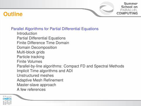
Parallel Algorithms for Partial Differential EquationsIntroductionPartial Differential EquationsFinite Difference Time DomainDomain DecompositionMulti-block gridsParticle trackingFinite VolumesParallel-by-line algorithms: Compact FD and Spectral MethodsImplicit Time algorithms and ADIUnstructured meshesAdaptive Mesh RefinementMaster-slave approachA few references
Outline
Parallel Algorithms for Partial Differential EquationsIntroductionPartial Differential EquationsFinite Difference Time DomainDomain DecompositionMulti-block gridsParticle trackingFinite VolumesParallel-by-line algorithms: Compact FD and Spectral MethodsImplicit Time algorithms and ADIUnstructured meshesAdaptive Mesh RefinementMaster-slave approachA few references
Parallel Algorithms
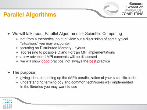
I We will talk about Parallel Algorithms for Scientific ComputingI not from a theoretical point of view but a discussion of some typical
“situations” you may encounterI focusing on Distributed Memory LayoutsI addressing to possible C and Fortran MPI implementationsI a few advanced MPI concepts will be discussedI we will show good practice, not always the best practice
I The purposeI giving ideas for setting up the (MPI) parallelization of your scientific codeI understanding terminology and common techniques well implemented
in the libraries you may want to use
Introduction
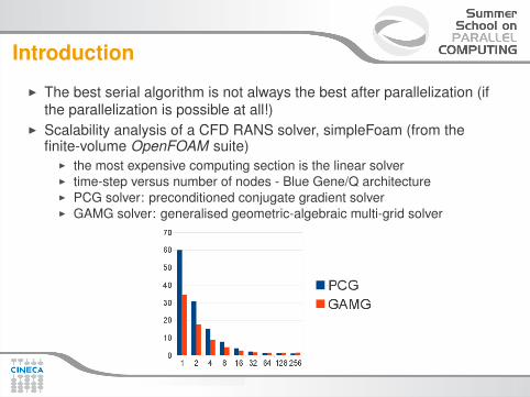
I The best serial algorithm is not always the best after parallelization (ifthe parallelization is possible at all!)
I Scalability analysis of a CFD RANS solver, simpleFoam (from thefinite-volume OpenFOAM suite)
I the most expensive computing section is the linear solverI time-step versus number of nodes - Blue Gene/Q architectureI PCG solver: preconditioned conjugate gradient solverI GAMG solver: generalised geometric-algebraic multi-grid solver
Introduction / 2
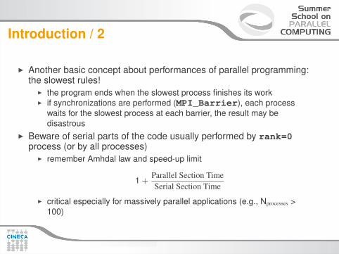
I Another basic concept about performances of parallel programming:the slowest rules!
I the program ends when the slowest process finishes its workI if synchronizations are performed (MPI_Barrier), each process
waits for the slowest process at each barrier, the result may bedisastrous
I Beware of serial parts of the code usually performed by rank=0process (or by all processes)
I remember Amhdal law and speed-up limit
1 +Parallel Section TimeSerial Section Time
I critical especially for massively parallel applications (e.g., Nprocesses >100)
Introduction / 3
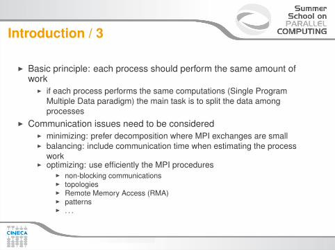
I Basic principle: each process should perform the same amount ofwork
I if each process performs the same computations (Single ProgramMultiple Data paradigm) the main task is to split the data amongprocesses
I Communication issues need to be consideredI minimizing: prefer decomposition where MPI exchanges are smallI balancing: include communication time when estimating the process
workI optimizing: use efficiently the MPI procedures
I non-blocking communicationsI topologiesI Remote Memory Access (RMA)I patternsI . . .
Introduction / 4
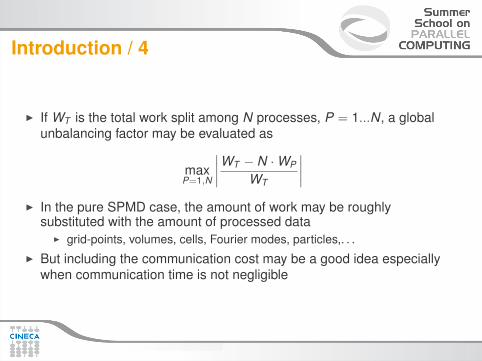
I If WT is the total work split among N processes, P = 1...N, a globalunbalancing factor may be evaluated as
maxP=1,N
∣∣∣∣WT − N ·WP
WT
∣∣∣∣I In the pure SPMD case, the amount of work may be roughly
substituted with the amount of processed dataI grid-points, volumes, cells, Fourier modes, particles,. . .
I But including the communication cost may be a good idea especiallywhen communication time is not negligible
Introduction / 5
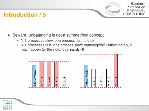
I Beware: unbalancing is not a symmetrical conceptI N-1 processes slow, one process fast: it is okI N-1 processes fast, one process slow: catastrophic! Unfortunately, it
may happen for the notorious rank=0
Programming models
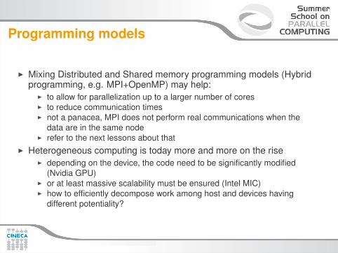
I Mixing Distributed and Shared memory programming models (Hybridprogramming, e.g. MPI+OpenMP) may help:
I to allow for parallelization up to a larger number of coresI to reduce communication timesI not a panacea, MPI does not perform real communications when the
data are in the same nodeI refer to the next lessons about that
I Heterogeneous computing is today more and more on the riseI depending on the device, the code need to be significantly modified
(Nvidia GPU)I or at least massive scalability must be ensured (Intel MIC)I how to efficiently decompose work among host and devices having
different potentiality?
Outline
Parallel Algorithms for Partial Differential EquationsIntroductionPartial Differential EquationsFinite Difference Time DomainDomain DecompositionMulti-block gridsParticle trackingFinite VolumesParallel-by-line algorithms: Compact FD and Spectral MethodsImplicit Time algorithms and ADIUnstructured meshesAdaptive Mesh RefinementMaster-slave approachA few references
Partial Differential Equations
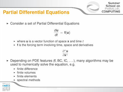
I Consider a set of Partial Differential Equations
dudt
= f(u)
I where u is a vector function of space x and time tI f is the forcing term involving time, space and derivatives
∂αu∂xα
I Depending on PDE features (f, BC, IC, . . . ), many algorithms may beused to numerically solve the equation, e.g.
I finite differenceI finite volumesI finite elementsI spectral methods
Outline
Parallel Algorithms for Partial Differential EquationsIntroductionPartial Differential EquationsFinite Difference Time DomainDomain DecompositionMulti-block gridsParticle trackingFinite VolumesParallel-by-line algorithms: Compact FD and Spectral MethodsImplicit Time algorithms and ADIUnstructured meshesAdaptive Mesh RefinementMaster-slave approachA few references

Finite Difference Time Domain
I Example: 1d convection-diffusion equation
dudt
= cdudx
+ νd2udx2
I Uniform discretization grid
xi = (i − 1) · dx ; i = 1,N
I Explicit Time advancement (e.g. Euler)
u(n+1)i − u(n)
idt
= c(
dudx
)(n)
i+ ν
(d2udx2
)(n)
i
I Need to evaluate derivatives on grid points
Finite Difference Time Domain
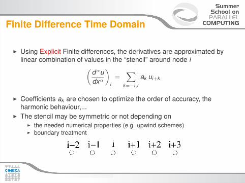
I Using Explicit Finite differences, the derivatives are approximated bylinear combination of values in the “stencil” around node i(
dαudxα
)i=
∑k=−l,r
ak ui+k
I Coefficients ak are chosen to optimize the order of accuracy, theharmonic behaviour,...
I The stencil may be symmetric or not depending onI the needed numerical properties (e.g. upwind schemes)I boundary treatment

Finite Difference Time Domain
I Example: 4-th order centered FD:(dudx
)i=
1/12ui−2 − 2/3ui−1 + 2/3ui+1 − 1/12ui+2
dx
I For points close to boundaries two approaches are commonI use adequate asymmetric stencil (hopefully preserving the numerical
properties), e.g.(dudx
)1=−25/12u1 + 4u2 − 3u3 + 4/3u4 − 1/4u5
dx(dudx
)2= ...
I use halo (ghost) regions to maintain the same internal scheme
Outline
Parallel Algorithms for Partial Differential EquationsIntroductionPartial Differential EquationsFinite Difference Time DomainDomain DecompositionMulti-block gridsParticle trackingFinite VolumesParallel-by-line algorithms: Compact FD and Spectral MethodsImplicit Time algorithms and ADIUnstructured meshesAdaptive Mesh RefinementMaster-slave approachA few references
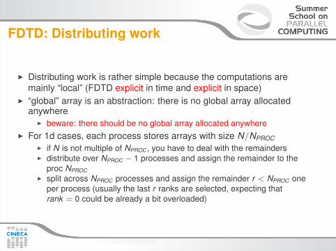
FDTD: Distributing work
I Distributing work is rather simple because the computations aremainly “local” (FDTD explicit in time and explicit in space)
I “global” array is an abstraction: there is no global array allocatedanywhere
I beware: there should be no global array allocated anywhereI For 1d cases, each process stores arrays with size N/NPROC
I if N is not multiple of NPROC , you have to deal with the remaindersI distribute over NPROC − 1 processes and assign the remainder to the
proc NPROCI split across NPROC processes and assign the remainder r < NPROC one
per process (usually the last r ranks are selected, expecting thatrank = 0 could be already a bit overloaded)
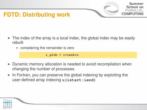
FDTD: Distributing work
I The index of the array is a local index, the global index may be easilyrebuilt
I considering the remainder is zero
i_glob = i+rank*n
I Dynamic memory allocation is needed to avoid recompilation whenchanging the number of processes
I In Fortran, you can preserve the global indexing by exploiting theuser-defined array indexing u(istart:iend)
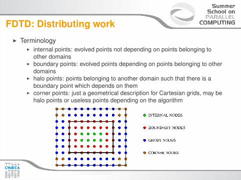
FDTD: Distributing workI Terminology
I internal points: evolved points not depending on points belonging toother domains
I boundary points: evolved points depending on points belonging to otherdomains
I halo points: points belonging to another domain such that there is aboundary point which depends on them
I corner points: just a geometrical description for Cartesian grids, may behalo points or useless points depending on the algorithm
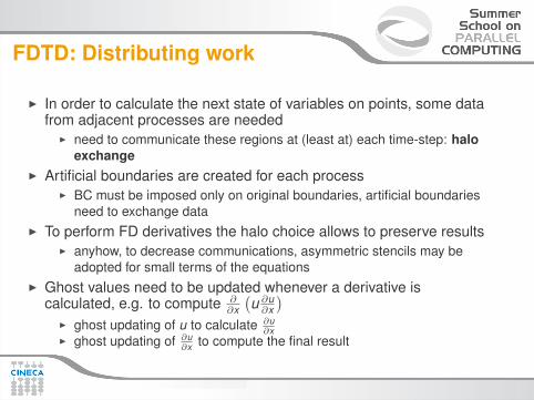
FDTD: Distributing work
I In order to calculate the next state of variables on points, some datafrom adjacent processes are needed
I need to communicate these regions at (least at) each time-step: haloexchange
I Artificial boundaries are created for each processI BC must be imposed only on original boundaries, artificial boundaries
need to exchange dataI To perform FD derivatives the halo choice allows to preserve results
I anyhow, to decrease communications, asymmetric stencils may beadopted for small terms of the equations
I Ghost values need to be updated whenever a derivative iscalculated, e.g. to compute ∂
∂x
(u ∂u∂x
)I ghost updating of u to calculate ∂u
∂xI ghost updating of ∂u
∂x to compute the final result
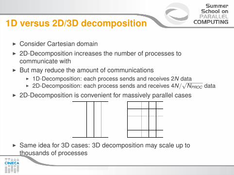
1D versus 2D/3D decomposition
I Consider Cartesian domainI 2D-Decomposition increases the number of processes to
communicate withI But may reduce the amount of communications
I 1D-Decomposition: each process sends and receives 2N dataI 2D-Decomposition: each process sends and receives 4N/
√NPROC data
I 2D-Decomposition is convenient for massively parallel cases
I Same idea for 3D cases: 3D decomposition may scale up tothousands of processes
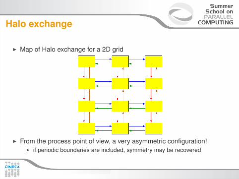
Halo exchange
I Map of Halo exchange for a 2D grid
I From the process point of view, a very asymmetric configuration!I if periodic boundaries are included, symmetry may be recovered
Cartesian Communicators
I Best practice: duplicate communicator to ensure communications willnever conflict
I required if the code is made into a component for use in other codesI But there is much more: MPI provides facilities to handle such
Cartesian TopologiesI Cartesian Communicators
I MPI_Cart_create, MPI_Cart_Shift. MPI_Cart_Coords,...I activating reordering, the MPI implementation may associate processes
to perform a better process placementI communicating trough sub-communicators (e.g., rows communicator,
columns communicator) may improve performancesI useful also to simplify coding

Clarifying halo exchange
I Let us clarify: boundary nodes are sent to neighbour processes to filltheir halo regions
I Remember: MPI common usage is two sided (the only way until MPI2)
I if process A sends data to process B, both A and B must be aware of itand call an MPI routine doing the right job
I one-sided communications (RMA) were introduced in MPI 2, very usefulbut probably not crucial for the basic domain decomposition
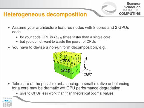
Heterogeneous decomposition
I Assume your architecture features nodes with 8 cores and 2 GPUseach
I for your code GPU is RGPU times faster than a single coreI but you do not want to waste the power of CPUs
I You have to devise a non-uniform decomposition, e.g.
I Take care of the possible unbalancing: a small relative unbalancingfor a core may be dramatic wrt GPU performance degradation
I give to CPUs less work than than theoretical optimal values

Heterogeneous decomposition / 2
I Of course, you need to write a code running two different pathsaccording to its rank
I A naive but effective approach: set NCOREXNODE and NGPUXNODE
GPU = .false.if(mod(n_rank,NCOREXNODE) .lt. NGPUXNODE) then
call acc_set_device(acc_device_nvidia)call acc_set_device_num(mod(n_rank,NCOREXNODE),acc_device_nvidia)print*,’n_rank: ’,n_rank,’ tries to set GPU: ’,mod(n_rank,NCOREXNODE)my_device = acc_get_device_num(acc_device_nvidia)print*,’n_rank: ’,n_rank,’ is using device: ’,my_deviceprint*,’Set GPU to true for rank: ’,n_rankGPU = .true.
endif........if(GPU) then; call var_k_eval_acc(ik) ; else; call var_k_eval_omp(ik) ; endifif(GPU) then; call update_var_k_mpi_acc() ; else; call update_var_k_mpi_omp() ; endifif(GPU) then; call bc_var_k_acc() ; else; call bc_var_k_omp() ; endifif(GPU) then; call rhs_k_eval_acc() ; else; call rhs_k_eval_omp() ; endif........
I use MPI_Comm_split to be more robust
Pattern SendRecv
I The basic pattern is based on MPI_SendrecvI e.g.: send to left and receive from right, and let MPI handling the
circular dependenciesI by the way, MPI_Sendrecv is commonly implemented byMPI_Isend, MPI_Irecv and a pair of MPI_Wait
I beware: send to left and receive from left cannot work, why?I For 2d decomposition, at least 4 calls are needed
I send to left and receive from rightI send to right and receive from leftI send to top and receive from bottomI send to bottom and receive from top
I 4 calls more if you need cornersI send LU and receive from RBI . . .
Non-blocking communications
I Non-blocking functions may improve performancesI reducing the artificial synchronization pointsI but the final performances have to be tested (and compared to theMPI_Sendrecv ones)
I A possible choice (consider neighbours ordered asdown,right,up,left)
do i=1,n_neighbourscall MPI_Irecv(....)
enddodo i=1,n_neighbours
call MPI_Send(....)enddocall MPI_Waitall(....) ! wait receive non-blocking calls
I Does not perform well in practice. Why?
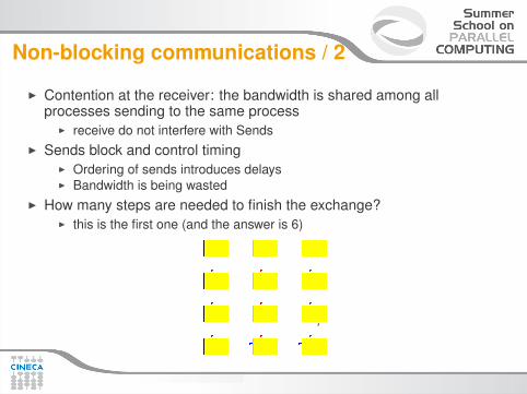
Non-blocking communications / 2
I Contention at the receiver: the bandwidth is shared among allprocesses sending to the same process
I receive do not interfere with SendsI Sends block and control timing
I Ordering of sends introduces delaysI Bandwidth is being wasted
I How many steps are needed to finish the exchange?I this is the first one (and the answer is 6)
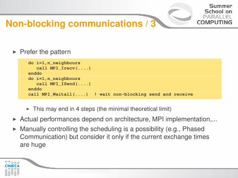
Non-blocking communications / 3
I Prefer the pattern
do i=1,n_neighbourscall MPI_Irecv(....)
enddodo i=1,n_neighbours
call MPI_ISend(....)enddocall MPI_Waitall(....) ! wait non-blocking send and receive
I This may end in 4 steps (the minimal theoretical limit)
I Actual performances depend on architecture, MPI implementation,...I Manually controlling the scheduling is a possibility (e.g., Phased
Communication) but consider it only if the current exchange timesare huge
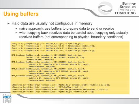
Using buffersI Halo data are usually not contiguous in memory
I naive approach: use buffers to prepare data to send or receiveI when copying back received data be careful about copying only actually
received buffers (not corresponding to physical boundary conditions)
for(j = 1; j<=mymsize_y; j++) buffer_s_rl[j-1] = T[stride_y+j];for(j = 1; j<=mymsize_y; j++) buffer_s_lr[j-1] = T[mymsize_x*stride_y+j];for(i = 1; i<=mymsize_x; i++) buffer_s_tb[i-1] = T[stride_y*i+1];for(i = 1; i<=mymsize_x; i++) buffer_s_bt[i-1] = T[stride_y*i+mymsize_y];
MPI_Sendrecv(buffer_s_rl, mymsize_y, MPI_DOUBLE, dest_rl, tag,buffer_r_rl, mymsize_y, MPI_DOUBLE, source_rl, tag,cartesianComm, &status);
MPI_Sendrecv(buffer_s_lr, mymsize_y, MPI_DOUBLE, dest_lr, tag+1,buffer_r_lr, mymsize_y, MPI_DOUBLE, source_lr, tag+1,cartesianComm, &status);
MPI_Sendrecv(buffer_s_tb, mymsize_x, MPI_DOUBLE, dest_tb, tag+2,buffer_r_tb, mymsize_x, MPI_DOUBLE, source_tb, tag+2,cartesianComm, &status);
MPI_Sendrecv(buffer_s_bt, mymsize_x, MPI_DOUBLE, dest_bt, tag+3,buffer_r_bt, mymsize_x, MPI_DOUBLE, source_bt, tag+3,cartesianComm, &status);
if(source_rl>=0)for(j=1;j<=mymsize_y;j++)T[stride_y*(mymsize_x+1)+j]=buffer_r_rl[j-1];if(source_lr>=0)for(j=1;j<=mymsize_y;j++)T[j]=buffer_r_lr[j-1];if(source_tb>=0)for(i=1;i<=mymsize_x;i++)T[stride_y*i+mymsize_y+1]=buffer_r_tb[i-1];if(source_bt>=0)for(i=1;i<=mymsize_x;i++)T[stride_y*i]=buffer_r_bt[i-1];

Fortran alternative
I Using Fortran, buffers may be automatically managed bythe language
I unlike C counter-parts, Fortran pointers may point to non-contiguousmemory regions
buffer_s_rl => T(1,1:mymsize_y)buffer_r_rl => T(mymsize_x+1:1:mymsize_y)call MPI_Sendrecv(buffer_s_rl, mymsize_y, MPI_DOUBLE_PRECISION, dest_rl, tag, &
buffer_r_rl, mymsize_y, MPI_DOUBLE_PRECISION, source_rl, tag, &cartesianComm, status, ierr)
I Or you can trust the array syntaxI probably the compiler will create the buffersI and in some cases, it may fail, why?
call MPI_Sendrecv(T(1,1:mymsize_y), mymsize_y, MPI_DOUBLE_PRECISION, dest_rl, tag, &T(mymsize_x+1:1:mymsize_y), mymsize_y, MPI_DOUBLE_PRECISION, source_rl, tag, &cartesianComm, status, ierr)
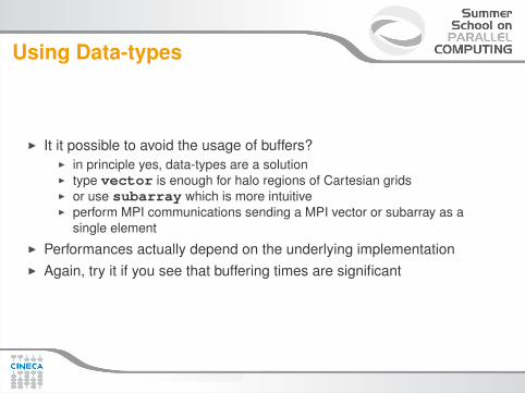
Using Data-types
I It it possible to avoid the usage of buffers?I in principle yes, data-types are a solutionI type vector is enough for halo regions of Cartesian gridsI or use subarray which is more intuitiveI perform MPI communications sending a MPI vector or subarray as a
single elementI Performances actually depend on the underlying implementationI Again, try it if you see that buffering times are significant
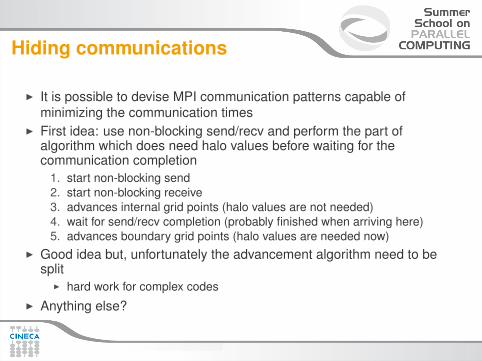
Hiding communications
I It is possible to devise MPI communication patterns capable ofminimizing the communication times
I First idea: use non-blocking send/recv and perform the part ofalgorithm which does need halo values before waiting for thecommunication completion
1. start non-blocking send2. start non-blocking receive3. advances internal grid points (halo values are not needed)4. wait for send/recv completion (probably finished when arriving here)5. advances boundary grid points (halo values are needed now)
I Good idea but, unfortunately the advancement algorithm need to besplit
I hard work for complex codesI Anything else?
Hiding communications / 2
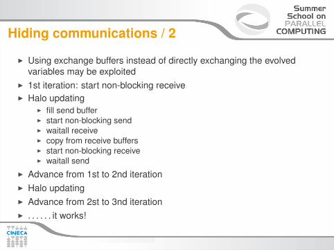
I Using exchange buffers instead of directly exchanging the evolvedvariables may be exploited
I 1st iteration: start non-blocking receiveI Halo updating
I fill send bufferI start non-blocking sendI waitall receiveI copy from receive buffersI start non-blocking receiveI waitall send
I Advance from 1st to 2nd iterationI Halo updatingI Advance from 2st to 3nd iterationI . . . . . . it works!
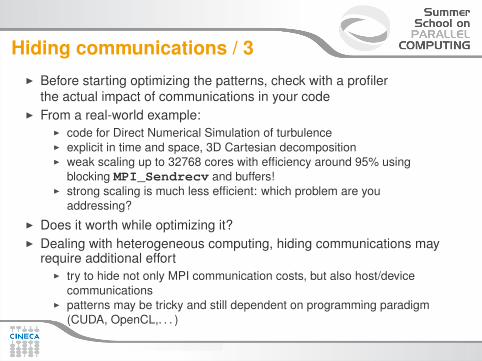
Hiding communications / 3I Before starting optimizing the patterns, check with a profiler
the actual impact of communications in your codeI From a real-world example:
I code for Direct Numerical Simulation of turbulenceI explicit in time and space, 3D Cartesian decompositionI weak scaling up to 32768 cores with efficiency around 95% using
blocking MPI_Sendrecv and buffers!I strong scaling is much less efficient: which problem are you
addressing?I Does it worth while optimizing it?I Dealing with heterogeneous computing, hiding communications may
require additional effortI try to hide not only MPI communication costs, but also host/device
communicationsI patterns may be tricky and still dependent on programming paradigm
(CUDA, OpenCL,. . . )
Collective and Reductions
I Even in explicit algorithms, exchanging halos is not enough to carryon the computation
I often, you need to perform “reductions”, requiring collectivecommunications
I Consider you want to check the behaviour of “residuals” (norm offield difference among two consecutive time-steps)
I MPI_Allreduce will help youI The situation is more critical for implicit algorithms
I the impact of collective communications may the actual bottle-neck ofthe whole code (see later)
Collective and Reductions / 2
I Up to MPI-2, collective communications were always blockingI to perform non-blocking collectives you had to use threads (Hybrid
Programming)I Using MPI-3 non-blocking collective procedures are available
I check if your MPI implementation supports MPI-3I anyhow, the usage of threads may be still a good option for other
reasons (again, study Hybrid Programming)I But the problem is that, often, collective operations must be executed
and finished before going on with the computationI select carefully the algorithm to implement
Outline
Parallel Algorithms for Partial Differential EquationsIntroductionPartial Differential EquationsFinite Difference Time DomainDomain DecompositionMulti-block gridsParticle trackingFinite VolumesParallel-by-line algorithms: Compact FD and Spectral MethodsImplicit Time algorithms and ADIUnstructured meshesAdaptive Mesh RefinementMaster-slave approachA few references
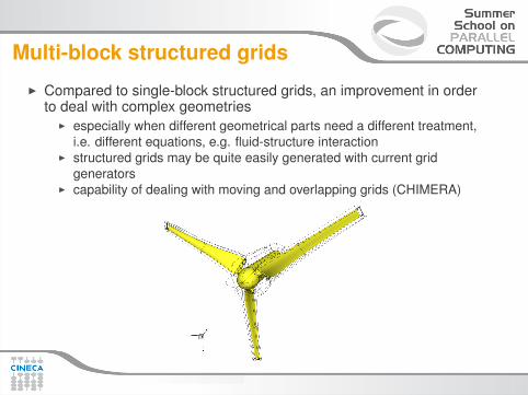
Multi-block structured grids
I Compared to single-block structured grids, an improvement in orderto deal with complex geometries
I especially when different geometrical parts need a different treatment,i.e. different equations, e.g. fluid-structure interaction
I structured grids may be quite easily generated with current gridgenerators
I capability of dealing with moving and overlapping grids (CHIMERA)
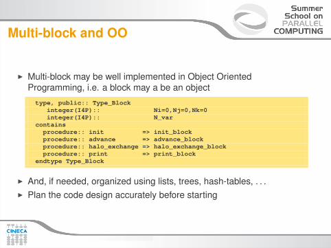
Multi-block and OO
I Multi-block may be well implemented in Object OrientedProgramming, i.e. a block may a be an object
type, public:: Type_Blockinteger(I4P):: Ni=0,Nj=0,Nk=0integer(I4P):: N_var
containsprocedure:: init => init_blockprocedure:: advance => advance_blockprocedure:: halo_exchange => halo_exchange_blockprocedure:: print => print_block
endtype Type_Block
I And, if needed, organized using lists, trees, hash-tables, . . .I Plan the code design accurately before starting
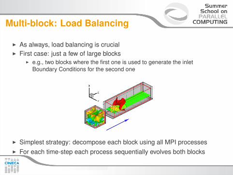
Multi-block: Load Balancing
I As always, load balancing is crucialI First case: just a few of large blocks
I e.g., two blocks where the first one is used to generate the inletBoundary Conditions for the second one
I Simplest strategy: decompose each block using all MPI processesI For each time-step each process sequentially evolves both blocks
Multi-block: Load Balancing / 2
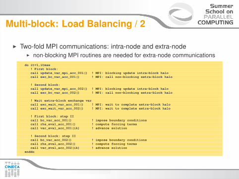
I Two-fold MPI communications: intra-node and extra-nodeI non-blocking MPI routines are needed for extra-node communicationsdo it=1,itmax
! First block:call update_var_mpi_acc_001() ! MPI: blocking update intra-block halocall exc_bc_var_acc_001() ! MPI: call non-blocking extra-block halo
! Second block:call update_var_mpi_acc_002() ! MPI: blocking update intra-block halocall exc_bc_var_acc_002() ! MPI: call non-blocking extra-block halo
! Wait extra-block exchange varcall exc_wait_var_acc_001() ! MPI: wait to complete extra-block halocall exc_wait_var_acc_002() ! MPI: wait to complete extra-block halo
! First block: step IIcall bc_var_acc_001() ! impose boundary conditionscall rhs_eval_acc_001() ! compute forcing termscall var_eval_acc_001(ik) ! advance solution
! Second block: step IIcall bc_var_acc_002() ! impose boundary conditionscall rhs_eval_acc_002() ! compute forcing termscall var_eval_acc_002(ik) ! advance solution
enddo
Multi-block: Load Balancing / 3
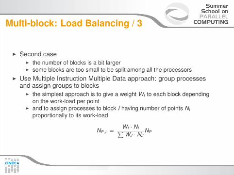
I Second caseI the number of blocks is a bit largerI some blocks are too small to be split among all the processors
I Use Multiple Instruction Multiple Data approach: group processesand assign groups to blocks
I the simplest approach is to give a weight WI to each block dependingon the work-load per point
I and to assign processes to block I having number of points NI
proportionally to its work-load
NP,I =WI · NI∑WJ · NJ
NP
Multi-block: Load Balancing / 4
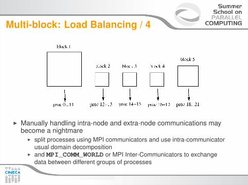
I Manually handling intra-node and extra-node communications maybecome a nightmare
I split processes using MPI communicators and use intra-communicatorusual domain decomposition
I and MPI_COMM_WORLD or MPI Inter-Communicators to exchangedata between different groups of processes
Multi-block: Load Balancing / 5
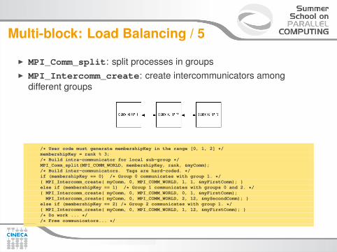
I MPI_Comm_split: split processes in groupsI MPI_Intercomm_create: create intercommunicators among
different groups
/* User code must generate membershipKey in the range [0, 1, 2] */membershipKey = rank % 3;/* Build intra-communicator for local sub-group */MPI_Comm_split(MPI_COMM_WORLD, membershipKey, rank, &myComm);/* Build inter-communicators. Tags are hard-coded. */if (membershipKey == 0) /* Group 0 communicates with group 1. */{ MPI_Intercomm_create( myComm, 0, MPI_COMM_WORLD, 1, 1, &myFirstComm); }else if (membershipKey == 1) /* Group 1 communicates with groups 0 and 2. */{ MPI_Intercomm_create( myComm, 0, MPI_COMM_WORLD, 0, 1, &myFirstComm);MPI_Intercomm_create( myComm, 0, MPI_COMM_WORLD, 2, 12, &mySecondComm); }
else if (membershipKey == 2) /* Group 2 communicates with group 1. */{ MPI_Intercomm_create( myComm, 0, MPI_COMM_WORLD, 1, 12, &myFirstComm); }/* Do work ... *//* Free communicators... */
Multi-block: Load Balancing / 5
I Third caseI the number of blocks is largeI and the sizes may be different
I Common strategyI avoid intra-block MPI parallelizationI if possible, use a shared-memory (OpenMP) intra-node parallelization
I Group blocks and assign groups to processesI obviously, the number of blocks must be greater or equal than the
number of processesI in any case, to ensure a proper load balancing an algorithm has to be
devised
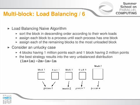
Multi-block: Load Balancing / 6
I Load Balancing Naive AlgorithmI sort the block in descending order according to their work-loadsI assign each block to a process until each process has one blockI assign each of the remaining blocks to the most unloaded block
I Consider an unlucky caseI 4 blocks having 1 million points each and 1 block having 2 million pointsI the best strategy results into the very unbalanced distribution(1m+1m)-2m-1m-1m
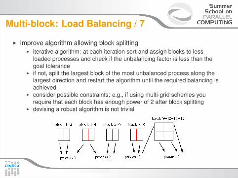
Multi-block: Load Balancing / 7
I Improve algorithm allowing block splittingI iterative algorithm: at each iteration sort and assign blocks to less
loaded processes and check if the unbalancing factor is less than thegoal tolerance
I if not, split the largest block of the most unbalanced process along thelargest direction and restart the algorithm until the required balancing isachieved
I consider possible constraints: e.g., if using multi-grid schemes yourequire that each block has enough power of 2 after block splitting
I devising a robust algorithm is not trivial
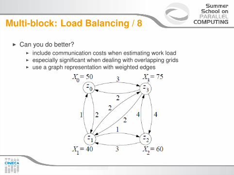
Multi-block: Load Balancing / 8
I Can you do better?I include communication costs when estimating work loadI especially significant when dealing with overlapping gridsI use a graph representation with weighted edges

Multi-block: Exchanging halo data
I Considering the “many blocks per process” configurationI before starting, store the blocks and process owners to communicate
with (send and/or receive)I at each time step exchange data using adequate patternsI no simple sendrecv structure may be used (sender and receivers are
not symmetrically distributed)I A possible pattern
1. copy from arrays to send buffers2. non-blocking recv from all relevant processes to buffers3. non-blocking send to all relevant processes to buffers4. loop over messages to receive
4.a waitany catches the first arrived message4.b copy received buffers to variables
5. waitall send
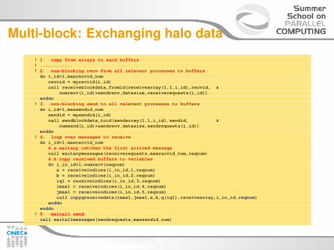
Multi-block: Exchanging halo data
! 1. copy from arrays to send buffers! ............! 2. non-blocking recv from all relevant processes to buffers
do i_id=1,maxrecvid_numrecvid = myrecvid(i_id)call receiveblockdata_fromid(receivearray(1,1,i_id),recvid, &
numrecv(i_id)*sendrecv_datasize,receiverequests(i_id))enddo
! 3. non-blocking send to all relevant processes to buffersdo i_id=1,maxsendid_num
sendid = mysendid(i_id)call sendblockdata_toid(sendarray(1,1,i_id),sendid, &
numsend(i_id)*sendrecv_datasize,sendrequests(i_id))enddo
! 4. loop over messages to receivedo i_id=1,maxrecvid_num
4.a waitany catches the first arrived messagecall waitanymessages(receiverequests,maxrecvid_num,reqnum)4.b copy received buffers to variablesdo i_in_id=1,numrecv(reqnum)
a = receiveindices(i_in_id,1,reqnum)b = receiveindices(i_in_id,2,reqnum)iq1 = receiveindices(i_in_id,3,reqnum)imax1 = receiveindices(i_in_id,4,reqnum)jmax1 = receiveindices(i_in_id,5,reqnum)call copyqreceivedata(imax1,jmax1,a,b,q(iq1),receivearray,i_in_id,reqnum)
enddoenddo
! 5. waitall sendcall waitallmessages(sendrequests,maxsendid_num)
Outline
Parallel Algorithms for Partial Differential EquationsIntroductionPartial Differential EquationsFinite Difference Time DomainDomain DecompositionMulti-block gridsParticle trackingFinite VolumesParallel-by-line algorithms: Compact FD and Spectral MethodsImplicit Time algorithms and ADIUnstructured meshesAdaptive Mesh RefinementMaster-slave approachA few references
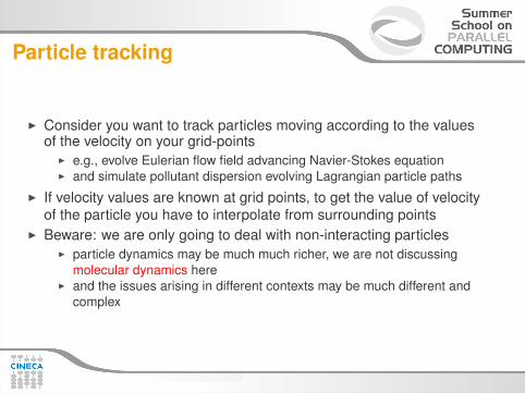
Particle tracking
I Consider you want to track particles moving according to the valuesof the velocity on your grid-points
I e.g., evolve Eulerian flow field advancing Navier-Stokes equationI and simulate pollutant dispersion evolving Lagrangian particle paths
I If velocity values are known at grid points, to get the value of velocityof the particle you have to interpolate from surrounding points
I Beware: we are only going to deal with non-interacting particlesI particle dynamics may be much much richer, we are not discussing
molecular dynamics hereI and the issues arising in different contexts may be much different and
complex
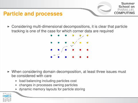
Particle and processes
I Considering multi-dimensional decompositions, it is clear that particletracking is one of the case for which corner data are required
I When considering domain decomposition, at least three issues mustbe considered with care
I load balancing including particles costI changes in processes owning particlesI dynamic memory layouts for particle storing

Particle and processes / 2
I Particle data need to be communicated from one process to anotherI reasonings about blocking/non-blocking communications and MPI
patterns still applyI If the cost of particle computing is high, the symmetry of Cartesian
load balancing could be not enough anymoreI in the simplest cases, symmetrically assigning a different amount of
points to processes may solve the problem (see heterogeneousdecomposition example)
I in the worst cases, e.g., when particle clustering occurs, no simplesymmetry is still available and the Cartesian Communicator is not theright choice
I graph topology? multi-block? unstructured grid?
Particle and processes / 3
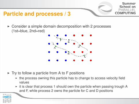
I Consider a simple domain decomposition with 2 processes(1st=blue, 2nd=red)
I Try to follow a particle from A to F positionsI the process owning this particle has to change to access velocity field
valuesI it is clear that process 1 should own the particle when passing trough A
and F, while process 2 owns the particle for C and D positions
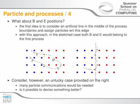
Particle and processes / 4I What about B and E positions?
I the first idea is to consider an artificial line in the middle of the processboundaries and assign particles wrt this edge
I with this approach, in the sketched case both B and E would belong tothe first process
I Consider, however, an unlucky case provided on the rightI many particle communications would be neededI is it possible to devise something better?
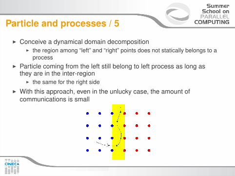
Particle and processes / 5
I Conceive a dynamical domain decompositionI the region among “left” and “right” points does not statically belongs to a
processI Particle coming from the left still belong to left process as long as
they are in the inter-regionI the same for the right side
I With this approach, even in the unlucky case, the amount ofcommunications is small
Particle and processes / 6
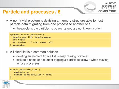
I A non trivial problem is devising a memory structure able to hostparticle data migrating from one process to another one
I the problem: the particles to be exchanged are not known a priori
typedef struct particle {double pos [3]; double mass;int type;int number; // char name [80];
} particle;
I A linked list is a common solutionI deleting an element from a list is easy moving pointersI include a name or a number tagging a particle to follow it when moving
across processes
struct particle_list {particle p;struct particle_list * next;
};
Particle and processes / 7
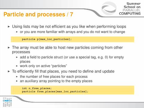
I Using lists may be not efficient as you like when performing loopsI or you are more familiar with arrays and you do not want to change
particle p[max_loc_particles];
I The array must be able to host new particles coming from otherprocesses
I add a field to particle struct (or use a special tag, e.g. 0) for emptyplaces
I work only on active “particles”I To efficiently fill that places, you need to define and update
I the number of free places for each processI an auxiliary array pointing to the empty places
int n_free_places;particle free_places[max_loc_particles];
Outline
Parallel Algorithms for Partial Differential EquationsIntroductionPartial Differential EquationsFinite Difference Time DomainDomain DecompositionMulti-block gridsParticle trackingFinite VolumesParallel-by-line algorithms: Compact FD and Spectral MethodsImplicit Time algorithms and ADIUnstructured meshesAdaptive Mesh RefinementMaster-slave approachA few references
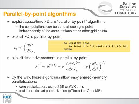
Parallel-by-point algorithmsI Explicit space/time FD are “parallel-by-point” algorithms
I the computations can be done at each grid pointindependently of the computations at the other grid points
I explicit FD is parallel-by-point:
ui ⇒(∂u∂x
)i
do i=istart,ienddu_dx(i) = 1./(2.*dx)*(u(i+1)-i(i-1))
enddo
I explicit time advancement is parallel-by-point:
u(n)i ⇒ u(n+1)
i = c(
dudx
)(n)
i+ ν
(d2udx2
)(n)
i
I By the way, these algorithms allow easy shared-memoryparallelizations
I core vectorization, using SSE or AVX unitsI multi-core thread parallelization (pThread or OpenMP)
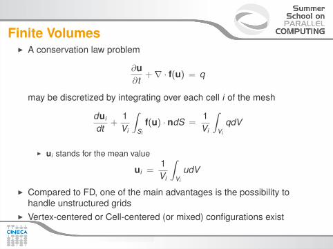
Finite VolumesI A conservation law problem
∂u∂t
+∇ · f(u) = q
may be discretized by integrating over each cell i of the mesh
dui
dt+
1Vi
∫Si
f(u) · ndS =1Vi
∫Vi
qdV
I ui stands for the mean value
ui =1Vi
∫Vi
udV
I Compared to FD, one of the main advantages is the possibility tohandle unstructured grids
I Vertex-centered or Cell-centered (or mixed) configurations exist
Finite Volumes / 2I To obtain a linear system, integrals must be expressed
in terms of mean valuesI For Volume integrals, midpoint rule is the basic option
qi =1Vi
∫Vi
qdV ' q(xi)
I For Surface integrals
1Vi
∑k
∫Si,k
f(u) · nkdS
interpolation is needed to obtain the functions values at quadraturepoints (face value ff ) starting from the values at computational nodes(cell values fP and fN )
ff = D · fP + (1− D) · fN
Finite Volumes / 3
I Finite Volume space discretization is parallel-by-point (but often timeadvancement is not)
I Interpolation is the most critical point wrt parallelismI Consider a simple FVM domain decomposition: each cell belongs
exactly to one processorI no inherent overlap for computational points
I Mesh faces can be grouped as followsI Internal faces, within a single processor meshI Boundary facesI Inter-processor boundary faces: faces used to be internal but are now
separate and represented on 2 CPUs. No face may belong to morethan 2 sub-domains
Finite Volumes / 4
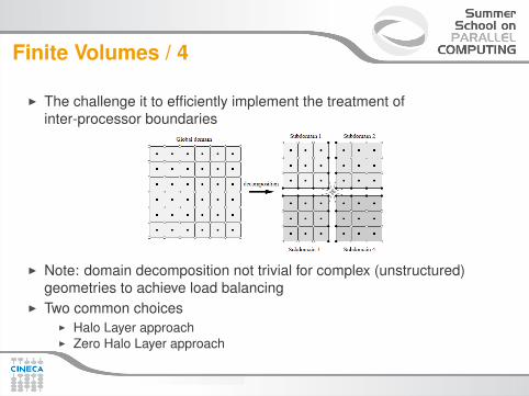
I The challenge it to efficiently implement the treatment ofinter-processor boundaries
I Note: domain decomposition not trivial for complex (unstructured)geometries to achieve load balancing
I Two common choicesI Halo Layer approachI Zero Halo Layer approach
FV: Halo Layer approach
I Consideringff = D · fP + (1− D) · fN
in parallel, fP and fN may live on different processorsI Traditionally, FVM parallelization uses halo layer approach (similar to
FD approach): data for cells next to a processor boundary isduplicated
I Halo layer covers all processor boundaries and is explicitly updatedthrough parallel communications calls
I Pro: Communications pattern is prescribed, only halo information isexchanged
I Con: Major impact on code design, all cell and face loops need torecognise and handle the presence of halo layer
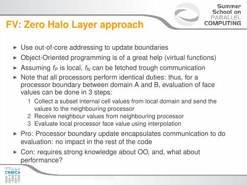
FV: Zero Halo Layer approach
I Use out-of-core addressing to update boundariesI Object-Oriented programming is of a great help (virtual functions)I Assuming fP is local, fN can be fetched trough communicationI Note that all processors perform identical duties: thus, for a
processor boundary between domain A and B, evaluation of facevalues can be done in 3 steps:
1 Collect a subset internal cell values from local domain and send thevalues to the neighbouring processor
2 Receive neighbour values from neighbouring processor3 Evaluate local processor face value using interpolation
I Pro: Processor boundary update encapsulates communication to doevaluation: no impact in the rest of the code
I Con: requires strong knowledge about OO, and, what aboutperformance?
Outline
Parallel Algorithms for Partial Differential EquationsIntroductionPartial Differential EquationsFinite Difference Time DomainDomain DecompositionMulti-block gridsParticle trackingFinite VolumesParallel-by-line algorithms: Compact FD and Spectral MethodsImplicit Time algorithms and ADIUnstructured meshesAdaptive Mesh RefinementMaster-slave approachA few references
Compact Finite Differences
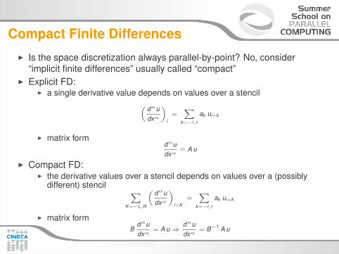
I Is the space discretization always parallel-by-point? No, consider“implicit finite differences” usually called “compact”
I Explicit FD:I a single derivative value depends on values over a stencil(
dαudxα
)i=
∑k=−l,r
ak ui+k
I matrix formdαudxα
= A u
I Compact FD:I the derivative values over a stencil depends on values over a (possibly
different) stencil ∑K=−L,R
(dαudxα
)i+K
=∑
k=−l,r
ak ui+k
I matrix formB
dαudxα
= A u ⇒dαudxα
= B−1 A u
Compact Finite Differences
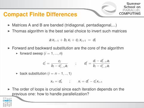
I Matrices A and B are banded (tridiagonal, pentadiagonal,...)I Thomas algorithm is the best serial choice to invert such matrices
a xi−1 + bi xi + ci xi+1 = di
I Forward and backward substitution are the core of the algorithmI forward sweep (i = 1, ..., n)
c′i =ci
bi − c′i−1ai; d ′i =
di − d ′i−1ai
bi − c′i−1ai
I back substitution (i = n − 1, .., 1)
xn = d ′n ; xi = d ′i − c′i xi+1
I The order of loops is crucial since each iteration depends on theprevious one: how to handle parallelization?
Compact Finite Differences / 2
I Considering a 3D problem, use a 2D domain decompositionI When deriving along one direction, e.g. x-direction, transpose data
so that the decomposition acts on the other two directions, e.g. y andz
I For each y and z, the entire x derivatives may be evaluated inparallel by Thomas algorithm
I Compact FD is an example of “parallel-by-line” algorithmI Transpose data, i.e. MPI_Alltoall, has a (significant) cost:
I may be slowI is only “out of place”, beware of memory usage
I Other possibilities?I use another algorithm instead of Thomas one: e.g., cyclic reduction
may be better parallelizedI compare the performances with the Transpose+Thomas choice
Spectral Methods
I Another class of methods, based on (Fast) Fourier TransformI may be very accurateI some equations get strongly simplified with this approach
I Considering 3D problems, a 3D-FFT is performed sequentiallytransforming x , y and z direction
I Since FFT usually employs a serial algorithm, a 3D-FFT is anotherexample of “parallel-by-line” algorithm
I Transposition of data is the common way to handle parallelization ofFFT
I Study carefully your FFT libraryI FFTW is the widespread library, also providing MPI facilities and a
specialized MPI transpose routine capable of handling in-place dataI often vendors FFTs perform better
Outline
Parallel Algorithms for Partial Differential EquationsIntroductionPartial Differential EquationsFinite Difference Time DomainDomain DecompositionMulti-block gridsParticle trackingFinite VolumesParallel-by-line algorithms: Compact FD and Spectral MethodsImplicit Time algorithms and ADIUnstructured meshesAdaptive Mesh RefinementMaster-slave approachA few references
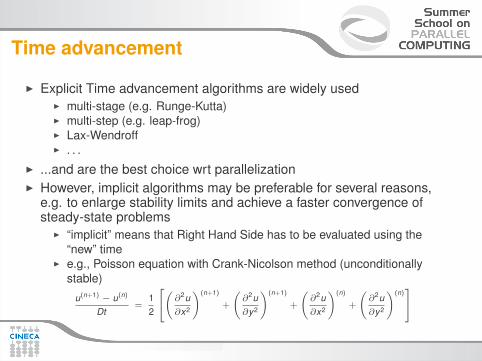
Time advancement
I Explicit Time advancement algorithms are widely usedI multi-stage (e.g. Runge-Kutta)I multi-step (e.g. leap-frog)I Lax-WendroffI . . .
I ...and are the best choice wrt parallelizationI However, implicit algorithms may be preferable for several reasons,
e.g. to enlarge stability limits and achieve a faster convergence ofsteady-state problems
I “implicit” means that Right Hand Side has to be evaluated using the“new” time
I e.g., Poisson equation with Crank-Nicolson method (unconditionallystable)
u(n+1) − u(n)
Dt=
12
(∂2u∂x2
)(n+1)
+
(∂2u∂y2
)(n+1)
+
(∂2u∂x2
)(n)
+
(∂2u∂y2
)(n)
Time advancement
I Adopting the matrix form
A u(n+1) = B u(n)
it results that a linear system has to be solvedI Thomas algorithm is not applicable because the bands of matrix are
not contiguousI The direct solution is costly, while an efficient approximate solutions
may be obtained using iterative methods, e.g. conjugate gradientmethod
I Anyhow, the shape of A may be simple, how to exploit it?

ADI
I Some numerical schemes strongly simplify the parallelizationI Alternating direction implicit method (ADI)
u(n+1/2) − u(n)
Dt= 0.5
[(∂2u∂x2
)(n+1/2)
+
(∂2u∂y2
)(n)]
u(n+1) − u(n+1/2)
Dt= 0.5
[(∂2u∂x2
)(n+1/2)
+
(∂2u∂y2
)(n+1)]I The system is symmetric and tridiagonal and may be solved using
Thomas algorithmI handling parallelization is not difficult transposing data
Outline
Parallel Algorithms for Partial Differential EquationsIntroductionPartial Differential EquationsFinite Difference Time DomainDomain DecompositionMulti-block gridsParticle trackingFinite VolumesParallel-by-line algorithms: Compact FD and Spectral MethodsImplicit Time algorithms and ADIUnstructured meshesAdaptive Mesh RefinementMaster-slave approachA few references
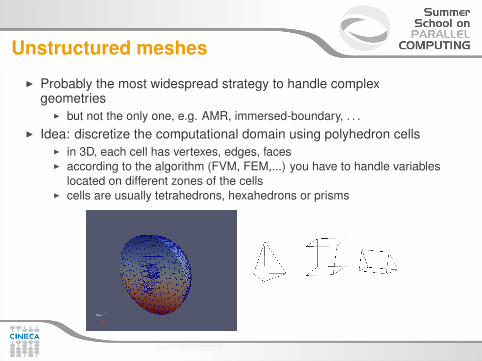
Unstructured meshes
I Probably the most widespread strategy to handle complexgeometries
I but not the only one, e.g. AMR, immersed-boundary, . . .I Idea: discretize the computational domain using polyhedron cells
I in 3D, each cell has vertexes, edges, facesI according to the algorithm (FVM, FEM,...) you have to handle variables
located on different zones of the cellsI cells are usually tetrahedrons, hexahedrons or prisms
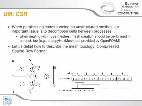
UM: CSR
I When parallelizing codes running on unstructured meshes, animportant issue is to decompose cells between processes
I when dealing with huge meshes, mesh creation should be performed inparallel, too (e.g., snappyHexMesh tool provided by OpenFOAM)
I Let us detail how to describe the mesh topology: CompressedSparse Row Format
UM: decomposition
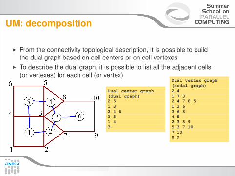
I From the connectivity topological description, it is possible to buildthe dual graph based on cell centers or on cell vertexes
I To describe the dual graph, it is possible to list all the adjacent cells(or vertexes) for each cell (or vertex)
Dual center graph(dual graph)2 51 32 4 63 51 43
Dual vertex graph(nodal graph)2 41 7 32 4 7 8 51 3 63 6 84 52 3 8 95 3 7 107 108 9
UM: decomposition
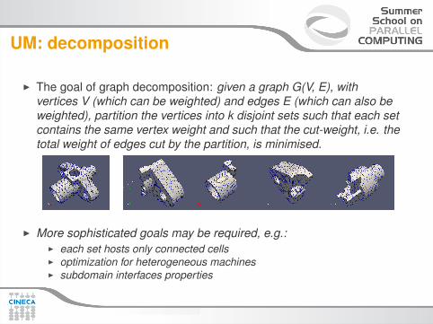
I The goal of graph decomposition: given a graph G(V, E), withvertices V (which can be weighted) and edges E (which can also beweighted), partition the vertices into k disjoint sets such that each setcontains the same vertex weight and such that the cut-weight, i.e. thetotal weight of edges cut by the partition, is minimised.
I More sophisticated goals may be required, e.g.:I each set hosts only connected cellsI optimization for heterogeneous machinesI subdomain interfaces properties
Libraries and METIS
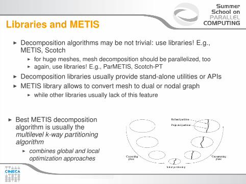
I Decomposition algorithms may be not trivial: use libraries! E.g.,METIS, Scotch
I for huge meshes, mesh decomposition should be parallelized, tooI again, use libraries! E.g., ParMETIS, Scotch-PT
I Decomposition libraries usually provide stand-alone utilities or APIsI METIS library allows to convert mesh to dual or nodal graph
I while other libraries usually lack of this feature
I Best METIS decompositionalgorithm is usually themultilevel k-way partitioningalgorithm
I combines global and localoptimization approaches
Scotch
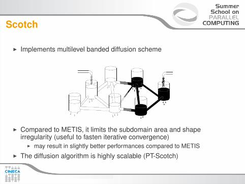
I Implements multilevel banded diffusion scheme
I Compared to METIS, it limits the subdomain area and shapeirregularity (useful to fasten iterative convergence)
I may result in slightly better performances compared to METISI The diffusion algorithm is highly scalable (PT-Scotch)
Outline
Parallel Algorithms for Partial Differential EquationsIntroductionPartial Differential EquationsFinite Difference Time DomainDomain DecompositionMulti-block gridsParticle trackingFinite VolumesParallel-by-line algorithms: Compact FD and Spectral MethodsImplicit Time algorithms and ADIUnstructured meshesAdaptive Mesh RefinementMaster-slave approachA few references
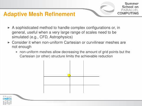
Adaptive Mesh Refinement
I A sophisticated method to handle complex configurations or, ingeneral, useful when a very large range of scales need to besimulated (e.g., CFD, Astrophysics)
I Consider it when non-uniform Cartesian or curvilinear meshes arenot enough
I non-uniform meshes allow decreasing the amount of grid points but theCartesian (or other) structure limits the achievable reduction
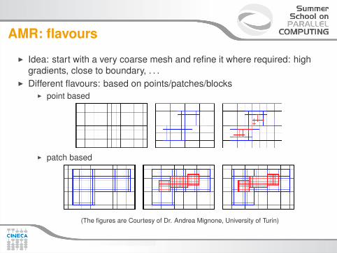
AMR: flavours
I Idea: start with a very coarse mesh and refine it where required: highgradients, close to boundary, . . .
I Different flavours: based on points/patches/blocksI point based
I patch based
(The figures are Courtesy of Dr. Andrea Mignone, University of Turin)
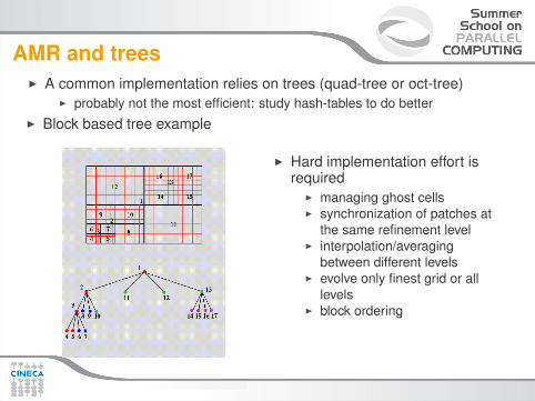
AMR and treesI A common implementation relies on trees (quad-tree or oct-tree)
I probably not the most efficient: study hash-tables to do betterI Block based tree example
I Hard implementation effort isrequired
I managing ghost cellsI synchronization of patches at
the same refinement levelI interpolation/averaging
between different levelsI evolve only finest grid or all
levelsI block ordering
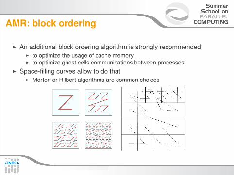
AMR: block ordering
I An additional block ordering algorithm is strongly recommendedI to optimize the usage of cache memoryI to optimize ghost cells communications between processes
I Space-filling curves allow to do thatI Morton or Hilbert algorithms are common choices
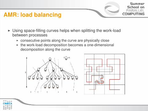
AMR: load balancing
I Using space-filling curves helps when splitting the work-loadbetween processes
I consecutive points along the curve are physically closeI the work-load decomposition becomes a one-dimensional
decomposition along the curve
AMR: libraries
I Before re-inventing the wheel check if one of the existing AMRlibraries is to your satisfaction
I PARAMESH - http://www.physics.drexel.edu/ olson/paramesh
I SAMRAI - https://computation.llnl.gov/casc/SAMRAI/
I p4est - http://www.p4est.org/
I Chombo - https://commons.lbl.gov/display/chombo/Chombo
Outline
Parallel Algorithms for Partial Differential EquationsIntroductionPartial Differential EquationsFinite Difference Time DomainDomain DecompositionMulti-block gridsParticle trackingFinite VolumesParallel-by-line algorithms: Compact FD and Spectral MethodsImplicit Time algorithms and ADIUnstructured meshesAdaptive Mesh RefinementMaster-slave approachA few references
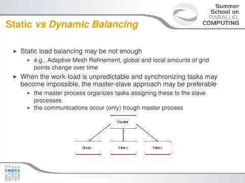
Static vs Dynamic Balancing
I Static load balancing may be not enoughI e.g., Adaptive Mesh Refinement, global and local amounts of grid
points change over timeI When the work-load is unpredictable and synchronizing tasks may
become impossible, the master-slave approach may be preferableI the master process organizes tasks assigning these to the slave
processesI the communications occur (only) trough master process
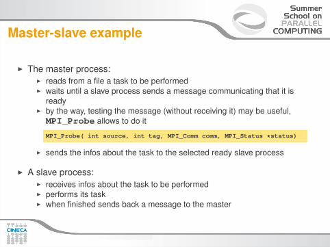
Master-slave example
I The master process:I reads from a file a task to be performedI waits until a slave process sends a message communicating that it is
readyI by the way, testing the message (without receiving it) may be useful,MPI_Probe allows to do it
MPI_Probe( int source, int tag, MPI_Comm comm, MPI_Status *status)
I sends the infos about the task to the selected ready slave process
I A slave process:I receives infos about the task to be performedI performs its taskI when finished sends back a message to the master
Outline
Parallel Algorithms for Partial Differential EquationsIntroductionPartial Differential EquationsFinite Difference Time DomainDomain DecompositionMulti-block gridsParticle trackingFinite VolumesParallel-by-line algorithms: Compact FD and Spectral MethodsImplicit Time algorithms and ADIUnstructured meshesAdaptive Mesh RefinementMaster-slave approachA few references
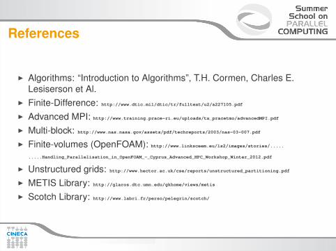
References
I Algorithms: “Introduction to Algorithms”, T.H. Cormen, Charles E.Lesiserson et Al.
I Finite-Difference: http://www.dtic.mil/dtic/tr/fulltext/u2/a227105.pdf
I Advanced MPI: http://www.training.prace-ri.eu/uploads/tx_pracetmo/advancedMPI.pdf
I Multi-block: http://www.nas.nasa.gov/assets/pdf/techreports/2003/nas-03-007.pdf
I Finite-volumes (OpenFOAM): http://www.linksceem.eu/ls2/images/stories/.....
.....Handling_Parallelisation_in_OpenFOAM_-_Cyprus_Advanced_HPC_Workshop_Winter_2012.pdf
I Unstructured grids: http://www.hector.ac.uk/cse/reports/unstructured_partitioning.pdf
I METIS Library: http://glaros.dtc.umn.edu/gkhome/views/metis
I Scotch Library: http://www.labri.fr/perso/pelegrin/scotch/

Rights & Credits
These slides are c©CINECA 2013 and are released underthe Attribution-NonCommercial-NoDerivs (CC BY-NC-ND) CreativeCommons license, version 3.0.
Uses not allowed by the above license need explicit, writtenpermission from the copyright owner. For more information see:
http://creativecommons.org/licenses/by-nc-nd/3.0/