Parallel Group Mining Algorithms

Thesis submitted in partial fullfilment of the

requirements for the award of degree of

Master of technology

in

Computer Science and Engineering

By

Anshuman Tripathi

(07CS3024)

under the guidance of

Prof. Arobinda Gupta

Department of Computer Science and EngineeringIndian Institute of Technology

Kharagpur-721302

CERTIFICATE

This is to certify that this thesis entitled “Parallelizing Group Mining Algorithms” submit-

ted by Anshuman Tripathi (07CS3024), in partial fulfillment for the award of the degree

of Master of Technology, is a record of bona-fide research work carried out by him under

my supervision during the period 2011-2012.

In my opinion this work fulfills the requirements for which it has been submitted. To best

of my knowledge, this thesis has not been submitted to any other university or institution

for any degree or diploma.

Dr. Arobinda Gupta

Department of Computer Science and Engineering

Indian Institute of technology

Kharagpur.

Acknowledgement

It gives me a great pleasure to thank all the people who have greatly helped me during

the course of this project. Foremost, I express deep gratitude and thanks to my supervisor

Dr. Arobinda Gupta for helping me shape this work to its current form. His invaluable

suggestions have introduced me to a very interesting and dynamic field. He has been very

much responsible for ensuring that my work progressed smoothly and surely in the right

direction.

The co-operation extended by our beloved Faculty Advisor, Dr. Jayanta Mukopahdyay,

is gratefully acknowledged.

Last but not the least, I am grateful to my parents and all my friends for their constant

support, encouragement, and help in many different ways.

Anshuman Tripathi

Contents

1 Introduction 1

1.1 Motivation . . . . . . . . . . . . . . . . . . . . . . . . . . . . . . . . . . . . . 1

1.2 Objectives & Contributions . . . . . . . . . . . . . . . . . . . . . . . . . . . . 2

1.3 Overview . . . . . . . . . . . . . . . . . . . . . . . . . . . . . . . . . . . . . . 2

2 Background 3

2.1 Definitions . . . . . . . . . . . . . . . . . . . . . . . . . . . . . . . . . . . . . . 3

2.2 Algorithms . . . . . . . . . . . . . . . . . . . . . . . . . . . . . . . . . . . . . 5

2.3 Metrics . . . . . . . . . . . . . . . . . . . . . . . . . . . . . . . . . . . . . . . 5

2.4 Hadoop . . . . . . . . . . . . . . . . . . . . . . . . . . . . . . . . . . . . . . . 6

2.5 Related Work . . . . . . . . . . . . . . . . . . . . . . . . . . . . . . . . . . . . 7

3 Proposed Parallelization Schemes 9

3.1 Data Organization . . . . . . . . . . . . . . . . . . . . . . . . . . . . . . . . . 9

3.1.1 Original(Trace) Format . . . . . . . . . . . . . . . . . . . . . . . . . . 9

3.1.2 Matrix Format . . . . . . . . . . . . . . . . . . . . . . . . . . . . . . . 10

3.1.3 List Format . . . . . . . . . . . . . . . . . . . . . . . . . . . . . . . . . 10

3.2 Branch-wise Parallelization . . . . . . . . . . . . . . . . . . . . . . . . . . . . 10

3.2.1 Job . . . . . . . . . . . . . . . . . . . . . . . . . . . . . . . . . . . . . 11

3.2.2 Master Process . . . . . . . . . . . . . . . . . . . . . . . . . . . . . . . 11

3.2.3 Worker Process . . . . . . . . . . . . . . . . . . . . . . . . . . . . . . . 11

3.2.4 Algorithms . . . . . . . . . . . . . . . . . . . . . . . . . . . . . . . . . 12

3.3 Data Parallelization . . . . . . . . . . . . . . . . . . . . . . . . . . . . . . . . 12

3.3.1 Algorithms . . . . . . . . . . . . . . . . . . . . . . . . . . . . . . . . . 14

3.4 Memory Bounded Versions . . . . . . . . . . . . . . . . . . . . . . . . . . . . 14

3.4.1 Modification in Branch Parallelization . . . . . . . . . . . . . . . . . . 14

3.4.2 Selecting Optimal Value of T . . . . . . . . . . . . . . . . . . . . . . . 15

3.5 Design issues . . . . . . . . . . . . . . . . . . . . . . . . . . . . . . . . . . . . 16

3.5.1 Time Requirements . . . . . . . . . . . . . . . . . . . . . . . . . . . . 16

3.5.2 Data Storage Requirements . . . . . . . . . . . . . . . . . . . . . . . . 16

3.5.3 Network Congestion . . . . . . . . . . . . . . . . . . . . . . . . . . . . 17

3

4 Results 18

4.1 Datasets . . . . . . . . . . . . . . . . . . . . . . . . . . . . . . . . . . . . . . . 18

4.1.1 Artificial Data: dataset 1 . . . . . . . . . . . . . . . . . . . . . . . . . 18

4.1.2 Dartmouth Data: dataset 2 . . . . . . . . . . . . . . . . . . . . . . . . 19

4.2 Data preprocessing . . . . . . . . . . . . . . . . . . . . . . . . . . . . . . . . . 21

4.2.1 Map Phase . . . . . . . . . . . . . . . . . . . . . . . . . . . . . . . . . 21

4.2.2 Reduce Phase . . . . . . . . . . . . . . . . . . . . . . . . . . . . . . . . 21

4.2.3 Preprocessing Time . . . . . . . . . . . . . . . . . . . . . . . . . . . . 21

4.3 Parallel MGS with dataset 1 . . . . . . . . . . . . . . . . . . . . . . . . . . . 23

4.3.1 Unbounded Memory . . . . . . . . . . . . . . . . . . . . . . . . . . . . 23

4.3.2 Bounded Memory . . . . . . . . . . . . . . . . . . . . . . . . . . . . . 25

4.3.3 Discussion . . . . . . . . . . . . . . . . . . . . . . . . . . . . . . . . . . 27

4.4 Parallel MGC with dataset 1 . . . . . . . . . . . . . . . . . . . . . . . . . . . 27

4.4.1 Unbounded Memory . . . . . . . . . . . . . . . . . . . . . . . . . . . . 27

4.4.2 Bounded Memory . . . . . . . . . . . . . . . . . . . . . . . . . . . . . 30

4.4.3 Discussion . . . . . . . . . . . . . . . . . . . . . . . . . . . . . . . . . . 30

4.5 Effects of number of nodes with dataset . . . . . . . . . . . . . . . . . . . . . 31

4.6 Parallel MGS with dataset 2 . . . . . . . . . . . . . . . . . . . . . . . . . . . 31

4.6.1 Unbounded Memory . . . . . . . . . . . . . . . . . . . . . . . . . . . . 32

4.6.2 Bounded Memory . . . . . . . . . . . . . . . . . . . . . . . . . . . . . 34

4.6.3 Discussion . . . . . . . . . . . . . . . . . . . . . . . . . . . . . . . . . . 35

4.7 Parallel MGC with dataset 2 . . . . . . . . . . . . . . . . . . . . . . . . . . 35

4.7.1 Unbounded Memory . . . . . . . . . . . . . . . . . . . . . . . . . . . . 35

4.7.2 Bounded Memory . . . . . . . . . . . . . . . . . . . . . . . . . . . . . 36

4.7.3 Discussion . . . . . . . . . . . . . . . . . . . . . . . . . . . . . . . . . . 37

4.8 MAWA∗ to MA∗ . . . . . . . . . . . . . . . . . . . . . . . . . . . . . . . . . 37

4.9 Algorithm Parameters . . . . . . . . . . . . . . . . . . . . . . . . . . . . . . . 38

4.10 Discussions . . . . . . . . . . . . . . . . . . . . . . . . . . . . . . . . . . . . . 42

5 Conclusions 44

5.1 Limitations . . . . . . . . . . . . . . . . . . . . . . . . . . . . . . . . . . . . . 44

5.2 Future Work . . . . . . . . . . . . . . . . . . . . . . . . . . . . . . . . . . . . 44

4

List of Figures

3.1 States of worker process . . . . . . . . . . . . . . . . . . . . . . . . . . . . . . 12

3.2 Data splitting in data parallelization . . . . . . . . . . . . . . . . . . . . . . . 13

3.3 Speedup vs T . . . . . . . . . . . . . . . . . . . . . . . . . . . . . . . . . . . . 15

3.4 Storage requirements of data formats . . . . . . . . . . . . . . . . . . . . . . . 17

4.1 Close pairs in Dartmouth data . . . . . . . . . . . . . . . . . . . . . . . . . . 20

4.2 Preprocessing times . . . . . . . . . . . . . . . . . . . . . . . . . . . . . . . . 22

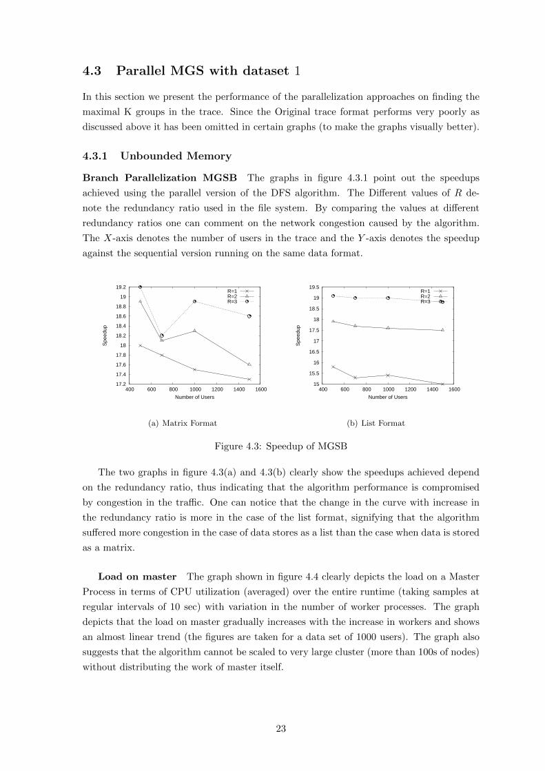
4.3 Speedup of MGSB . . . . . . . . . . . . . . . . . . . . . . . . . . . . . . . . . 23

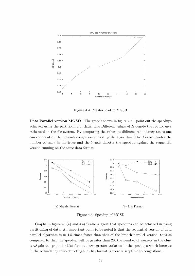
4.4 Master load in MGSB . . . . . . . . . . . . . . . . . . . . . . . . . . . . . . . 24

4.5 Speedup of MGSD . . . . . . . . . . . . . . . . . . . . . . . . . . . . . . . . . 24

4.6 Master load in MGSD . . . . . . . . . . . . . . . . . . . . . . . . . . . . . . . 25

4.7 Speedup for BMGSB with matrix format . . . . . . . . . . . . . . . . . . . . 26

4.8 Speedup for BMGSD with matrix format . . . . . . . . . . . . . . . . . . . . 26

4.9 Speedup of MGCB . . . . . . . . . . . . . . . . . . . . . . . . . . . . . . . . . 28

4.10 Master load in MGCB . . . . . . . . . . . . . . . . . . . . . . . . . . . . . . . 29

4.11 Speedup of MGCD . . . . . . . . . . . . . . . . . . . . . . . . . . . . . . . . . 29

4.12 Master load in MGCD . . . . . . . . . . . . . . . . . . . . . . . . . . . . . . . 30

4.13 Speedup for BMGCB with matrix format . . . . . . . . . . . . . . . . . . . . 31

4.14 Speedup for BMGCD with matrix format . . . . . . . . . . . . . . . . . . . . 32

4.15 Speedup Vs cluster size for unbounded case . . . . . . . . . . . . . . . . . . . 33

4.16 Speedup Vs cluster size for bounded case . . . . . . . . . . . . . . . . . . . . 34

4.17 Speedup of MGSB for dataset 2 . . . . . . . . . . . . . . . . . . . . . . . . . . 34

4.18 Speedup of MGSD for dataset 2 . . . . . . . . . . . . . . . . . . . . . . . . . . 35

4.19 Speedup of BMGSD algorithm on dataset 2 . . . . . . . . . . . . . . . . . . . 36

4.20 Speedup of MGCB for dataset 2 . . . . . . . . . . . . . . . . . . . . . . . . . 36

4.21 Speedup of MGCD algorithm with dataset 2 . . . . . . . . . . . . . . . . . . . 37

4.22 Speedup of BMGCD algorithm for dataset 2 . . . . . . . . . . . . . . . . . . . 38

4.23 Group search algorithm with MA∗ . . . . . . . . . . . . . . . . . . . . . . . . 39

4.24 Speedup with different memory bounds . . . . . . . . . . . . . . . . . . . . . 40

5

List of Tables

3.1 Load on master with T . . . . . . . . . . . . . . . . . . . . . . . . . . . . . . . 16

4.1 Runtime of sequential versions for dataset 1 . . . . . . . . . . . . . . . . . . . 20

4.2 Runtime of sequential versions for dataset 2 . . . . . . . . . . . . . . . . . . . 21

4.3 Run time in seconds . . . . . . . . . . . . . . . . . . . . . . . . . . . . . . . . 22

4.4 Speedup with memory bounds . . . . . . . . . . . . . . . . . . . . . . . . . . 27

4.5 Speed up with depth . . . . . . . . . . . . . . . . . . . . . . . . . . . . . . . . 39

4.6 Optimal depth . . . . . . . . . . . . . . . . . . . . . . . . . . . . . . . . . . . 39

4.7 Speedup with depth . . . . . . . . . . . . . . . . . . . . . . . . . . . . . . . . 40

4.8 Partial completion at different bounds . . . . . . . . . . . . . . . . . . . . . . 41

4.9 Optimal memory bounds . . . . . . . . . . . . . . . . . . . . . . . . . . . . . . 41

6

Abstract

Pattern Mining from user mobility traces over mobile networks is a well established com-

mercial problem which can be exploited for better performance and customization of user

applications. Most of the group mining algorithms deal with huge quantities of data and in

most of the cases perform similar computations on different data segments. The huge data

size, time consuming algorithms and repetitive computations can be used to produce par-

allel implementations of these algorithms. In the present work we study different schemes

for parallelizing some specific group mining algorithms, and comment on the scalability and

feasibility of parallelism achieved

Chapter 1

Introduction

Wireless networks and personalized mobile devices are deeply integrated and embedded in

our lives. It is very important to characterize the fundamental structure of wireless user

behavior in order to model, manage, leverage and design efficient mobile networks. Since

most of the users of a mobile network follow a daily routine with minor fluctuations over

a long interval of time, there lies an immensely powerful untapped possibility of network

performance optimization if the underlying statistical patterns and characteristics of users

can be conjectured. Pattern mining of user groups from mobility data is a very broad field

which may include various problems like mining mobility patterns, knowing hot spots, group

mining . . . etc.

Group pattern mining of mobile users is useful for several applications such as social

network analysis, businesses targeting groups of users, law enforcement, etc. The problem

of mining groups from a general user mobility model is a NP complete problem (reducible to

finding Max clique problem). Thus the algorithms designed to compute the Maximal groups

are either heuristics or require huge computational time. Algorithms have been developed

to proceed towards the optimal solutions gradually while maintaining a best solution every

time, so that the algorithm can be queried any time for the best result.

Parallelizing group mining algorithms is the practical aspect of mining procedures, the

aim being to attain appreciable speedups in huge machine clusters to bring the execution

time to practical limits. In the scope of present work we propose schemes to parallelize

these group mining algorithms and comment on the feasibility of the approaches.

1.1 Motivation

Parallelization of AI algorithms is a very well known field of research, which aims reduce

the time barrier for processes of AI engine to bring it to practical and bearable limits. As

multi-core architectures have become common, many approaches to use multiple cores to

do synchronized search have become popular, so that the brute computational power of

the cores can be tapped for faster execution of search algorithms. Keeping this in back-

drop, recent advances have also been made to use more than one machine that make up a

distributed computing system, to collaborate for speeding up the process of AI search.

Most of the Group Mining algorithms are like AI search algorithms that explore the

1

solutions space step by step in an orderly fashion. Although there are many AI search

methods that are both sound and complete but all the general search methods are prone

to long execution times pertaining to their exponential dependence on the input size. For

example one of the group mining algorithms used in this thesis that mines user groups based

on the size of the group takes ≈ 1.5 days to complete the computation for mobility data with

only 10000 users (practically the algorithm would have to deal with millions of users, and

the computations might have to be done several times a week or even day). This illustration

points out that no matter how effective the group mining algorithm is in identifying user

sets, it cant have practical use unless the runtime is reduced. Since most of the research

institutes and companies have huge clusters of machines at their disposal, parallelization of

mining algorithms pose a very interesting problem with many practical impacts.

1.2 Objectives & Contributions

The main objective of this work is to investigate practical parallelization schemes that can

be used to run the group mining algorithms on large scalable machine clusters. The parallel

algorithms shall be graded on metrics of scalability, and speedup achievable.

In this work we proposed two novel parallelization approaches and study their imple-

mentation on four different group mining approaches, while commenting on the feasibility

and scalability of the approaches. While parallelization is the main scope of the thesis, we

show that a simple change in the data format can bring an appreciable improvement in

the execution time of not only the parallel versions but also the sequential versions, thus

improving sequential baseline algorithms also. We also present a brief study of the tunable

parameters and their impact on the performance of the distributed system, and finally we

also present an objective comparison of parallel algorithms with memory bounds and those

with no bounds on the memory. We also present our results on real user mobility data

obtained from Dartmouth CRAWDAD project [6].

1.3 Overview

The rest of the thesis is organized into chapters. In Chapter 2 we give a brief pre-requisite

knowledge to understand the thesis better in form of basic group definitions and terms

used in the thesis. In the following Chapter 3 we give details of the parallelization schemes

proposed with hints on the implementations aspects on a Hadoop cluster. In Chapter 4 we

describe the simulation setup for the experiments conducted on different types of data-sets.

Finally we conclude the thesis in Chapter 5 by giving brief conclusions that could be arrived

at based on the experimental studies.

2

Chapter 2

Background

In this section we give brief background of terms used henceforth in this thesis and discuss

some of the related works.

2.1 Definitions

Groups As far as group mining from mobility pattern is considered a group is ‘recogniz-

able’ set of users with ‘important’ characteristics. Thus any generic definitions of group

should include following characteristics:-

• the group should be recognizable, i.e. definition of the group should unanimously be

able to distinguish between users that are part of the group and those that are not.

For this requirement most of the group definitions are based on the concept of cliques.

Other definitions based on concepts of n-core, n-clan . . . etc may find use in specific

places.

• the group should be important, i.e. the property on which the groups are formed

must have a direct relation with problem for which group mining is done. In most of

the cases group mining is done for applications like social network analysis, business

targeting . . . etc. Thus the definition and criteria of a user being in a group is highly

subjective to application at hand.

For a formal definition a Group is a set of users such that given any user ui from the

group it is close with all the other users in the set. This definition brings us to the definition

of closeness.

closeness is relation defined between a pair of users u1 and u2. They are said to close if

and only if they spend a threshold amount of time (Tthresh) being at most D distance apart.

Thus Tthresh and D are tunable parameters to suit various scenarios. More mathematically

closeness is defined as follows. Two users are said to be close if

α× Sphy + β × Svir = minwei (2.1)

where Sphy denotes the physical communication strength between the two users, Svir denotes

the virtual communication strength, and α, β, minwei are the application chosen parameters.

3

Physical communication strength can be calculated based on the amount of time that the

two users spent together on the basis of location-time data. The total weight of each edge

in the VG-graph is one such measure. Virtual communication strength can be calculated

based on the number of calls, messages, emails, etc between the users. Relative frequency

is an example of such a measure.

One can also define closeness in various other ways.

Group Pattern: A set of users form a group or group pattern if every two users of the set

are close.

The motivation behind such a definition is that if every two users of a set communicate

with each other strongly enough, then it is highly likely that they form a group and act as

a group for real.

The total number of maximal groups as per any given group definition can become very

large, highlighting the need for finding top K groups amongst the maximal groups. While

top K groups notion can vary from application to application, we consider two basic criteria

of coming up with Top K groups which can be of use in several applications, namely size

and coverage.

Size Applications may want to target the largest groups, in which case the top K groups

are the K maximal groups of largest size. Ties may be resolved based on some custom

criteria.

Coverage Applications may want to target most number of users via their group behavior,

in which case the number of users covered by the K groups is to be maximized.

There is an important difference between the two criteria. In case of the top K groups

with respect to size, each group of the K-set is independent, that is, if G is the only largest

sized group, then G belongs to the final K-set independent of whether any other maximal

group belongs to the K-set or not. However, in the case of top K groups with respect to

coverage, each group of the K-set is not independent, whether a given group belongs to the

final K-set or not is dependent on whether its involvement can increase the overall coverage

of the K-set. Hence, methods for finding the top K groups also differ based on the criterion.

Another important aspect of the group mining algorithms is that, they might be imple-

mented on less powerful nodes with serious limitations on the memory available. Thus two

sets of algorithms are important:-

Unbounded Memory : In these versions of algorithms, there is no bound on the mem-

ory practically usable by the algorithm. These algorithms are mostly based on an

underlying depth first search.

Bounded Memory : These versions are designed to work when there is a hard bound on

the amount of memory that can be used by the algorithms. Because if the memory

bounds these algorithms are generally slower in terms of the termination time, some

variants of this class are anytime algorithms in the sense that they can be queried

anytime during their execution for the best result until that point.

4

Based on the above bifurcations of group definitions and the algorithms, there are basi-

cally four type of group mining algorithms that are considered in the thesis viz:

1. Maximal Group Size Algorithms (MGS) : The unbounded memory version of algo-

rithm that mines top K groups based on the size of the individual groups.

2. Maximal Group Coverage Algorithm (MGC) : The unbounded memory version of

algorithm that mines top K groups that have the highest coverage of the users in the

trace.

3. Bounded Maximal Group Size Algorithm (BMGS): The unbounded memory version

for 1.

4. Bounded Maximal Group Coverage Algorithm (BMGC): The unbounded memory

version for 2.

2.2 Algorithms

In this section, we present the necessary background on best-first search strategies which

form the basis of proposed mining algorithms. A* is the most famous best-first search

technique, in which a set of nodes to be explored is maintained in a list called OPEN, and

the most promising node is chosen from OPEN each time, whose children are generated and

added to OPEN. The algorithm terminates when the chosen node is a goal node. Each node

has an f-value which denotes its promise. For example, in case of a maximization problem,

f-value of a node n indicates the possible output value when a goal node is reached through

n. A* gives optimal solution when the heuristic used for estimating the f-value overestimates

the actual output value achievable through the node (for a maximization problem).

A* however has two primary drawbacks:

1. It may run out of memory, and

2. It may take long time before giving the output, due to the large search spaces involved

with the optimization problems

Methods based on A* that can run within the given memory are proposed to handle the

memory limits. Anytime algorithms are proposed on top of A* to get solutions of good

quality quickly.MAWA* combines the techniques of MA* and AWA* to give good anytime

performance and work within the given memory limit. It successfully employs the depth

guided window technique of AWA* along with the least promising node removal technique

of MA* to come up with a complete memory-bounded anytime algorithm

2.3 Metrics

For gauging the performance of a parallel algorithm many metrics are important:-

5

Scalability This requirement means that the parallelization scheme should be able to scale

over large number of machines while efficiently being able to utilize the additional

computational power just as well as for the case when number of machines are lower.

Its a general observation that parallelization schemes suffer from some substantial

overhead that results in saturation of the computational efficacy of the system when

it reaches a certain size (in terms of the number of machines). Ideally an algorithm

should be able to achieve any finite amount of speedup by using a finite number of

machine nodes.

Speedup This metric measures the amount of absolute machine power that can be ex-

ploited in parallel by the distributed scheme. This is measured as the ratio of absolute

time required by sequential algorithm to the time required by the parallel algorithm

for execution of almost similar tasks.

speedup (µ) =Time on 1 machine

Time on n machines(2.2)

Ideally a parallel algorithm should have a speedup of µ = n where n is the number of

machines in the distributed cluster, However since in reality a parallel implementation

incurs overheads, the speedup is much less.

Stability This requirement of a parallel algorithm requires that the performance of the

algorithm should not be as independent of the input set as possible. Thus ideally a

parallel algorithm should not be based on specific properties in the input data so that

it delivers equal speedup and scalability over the entire input data space. However

in reality many parallelization schemes exploit the properties in the input data to

improve speedup and scalability.

2.4 Hadoop

The algorithms discussed in chapter 3 are all parallelization schemes that require access

of data for all the workers. Hadoop cluster has been used in the implementation of these

algorithms just for the sake of serving as a high performance distributed file system, other

than for its use in the pre-processing part (as discussed in chapter 3). Hadoop cluster has

many configurable parameters, those useful for the simulation results are:-

Workers The number of active workers can be configured in the cluster. Only the active

workers take part in the data storage organization. For the sake of simplicity all the

Hadoop workers are also the workers in the parallel computations and the Hadoop

master is the actual master in the algorithm runtime instance.

Redundancy Ratio (R) The redundancy ratio defines the number of copies of a data

block that are maintained in the hadoop cluster. Thus a value of R = 2 means all the

data blocks are stored have 2 copies at two separate locations. This parameter not

only guarantees some degree of fault tolerance but is pivot to the performance of the

distributed file system. Since higher values of R imply more number of copies, a read

6

query on the file system can be handled by R different sites, thus distributing the load

and reducing network congestion.

2.5 Related Work

With the advent of multi-core architectures and powerful machine clusters the aim of al-

gorithm design is gradually shifting from giving very high throughput on main frames to

being able to exploit the power of distributed systems. Many algorithms like brute depth

first search are inherently parallel while others like α-β pruning have to be analyzed and

modified. There are several reasons for this gradual shift:-

Multi-core architectures Since the advent of cheap and practical multi-core architec-

tures, increasing processor utilization has been the main aim of most software devel-

opment activities.

NP-problems Many problems for which heuristics are developed, fall in the class of NP

problems for which even the best known algorithms take exponential amount of time.

Although the barrier of time complexity can’t be broken, but being able to utilize

huge clusters bring the time requirements of practical problem within bearable limits.

AI problems Many artificial intelligence systems are by virtue of functionality and design

distributed in nature eg. Delay tolerant networks, Distributed mapping of resources

. . . etc.

A huge amount of work has been done previously in the field of parallelization of algo-

rithms. There have been many ground breaking designs in the field of AI algorithms that

utilize multi-core architectures eg. Principal Variation search (parallel version of α-β prun-

ing), Dynamic tree splitting (parallel version of α-β pruning and negascout search) . . . etc.

Many virtual machines have been designed that abstract the multi-core processor as single

core, and the parallelism is carried out internally at instruction level.

Map Reduce architecture [3] developed by Google is commercially used by many organi-

zations to perform computationally heavy tasks on machine clusters. Hadoop file system [1]

is developed manly to support the map-reduce architecture and is currently used by several

organizations.

There have even been programming languages like CUDA [8] developed by nVidia is a

highly scalable parallel programming language that can exploit a large number of GPU cores

to do fast floating point computations. Similarly ParaSail [9] developed by intel provides

parallel programming structures.

Distributed computing is also very useful in the field of medical science. Projects like

Folding@home [2] are massively distributed systems that utilize the power of idle machines

volunteered over the world to perform complex computations regarding protein folding

. . . etc, which can provide great insight to the cancer tissue culture. As mentioned ear-

lier pattern mining of user mobility models is a very important field. There have been many

works ( [7, 4]) in the area of pattern mining of user groups from mobility data. However to

7

make some practical use of group mining algorithms one must be able implement them on

distribute architectures, which is the main scope of the present work.

8

Chapter 3

Proposed Parallelization Schemes

There are basically two sequential algorithms that have been parallelized viz. finding the

top K maximal groups in terms of size and finding the set of K maximal groups which

maximizes coverage. Both these algorithms are an implementation of depth first search for

the groups with different end conditions. The parallel versions of these algorithms fall in

the following 2 approaches, detailed herein.

3.1 Data Organization

In this section we shall present the data organizations for which the parallel versions of the

algorithms have been studied. For a distributed algorithm the organization of data in the

cluster and the structure of the data play a very important role. Thus we propose three

basic data layouts for which the algorithm performance has been studied.

3.1.1 Original(Trace) Format

The format of the user trace on which the sequential version of the algorithm runs is as

follows:-

• The first line contains two integers the first one is the number of users (say N) for

which the trace is taken; the second one is the number of time segments (say T ) for

which the user positions are measured.

• This is followed by N lines where each line contains 2 timesT float values where the

values denote the x, y coordinates of the user in that time stamp.

This is a natural format to express real time trace data. Almost any metric pertaining to

the trace of the users can be computed from this format of data representation. The format

makes it computationally expensive to find whether two users are close. The computational

dependency between different blocks of data is quite high (to find whether two users are

close the data block for both of them shall be processed) this makes it difficult to distribute

the data among cluster nodes.

9

3.1.2 Matrix Format

In this format only the relevant information is retained in the data. The format is nothing

but pre-computed values for closeness of all the user pairs. The format is as follows:-

• The first line contains an Integer that represents the number of users N in the trace

• This is followed by N lines where each line is N characters long; each character is

either 0 or 1 indicating whether the user is close with that user.

This format makes the computation of the closeness of two users a constant time operation.

The data blocks are fairly independent thus the distributed storage of data is possible while

minimizing congestion.

The format is fairly specific to the algorithm at hand thus it loses many statistical

measures that could have been computed from the original trace format. Further the format

requires a preprocessing step (This step can however be supplemented by involving real time

closeness computation while trace generation, which is possible for the given definition of

closeness.) to convert the data from the original format to the matrix format which is in

itself a heavy computational job.

3.1.3 List Format

This format is derive from the above mentioned matrix format and aims at reducing the

data size for very sparse (or very dense) matrices. The format is:

• The first line consists of an integer that represents the number of users in the trace.

• The following lines have two integers that represent the ids of users which are close

(or not close).

The size of the data is expected to be less in case of sparse (or dense) matrix format.

The data format is still very much independent i.e. the data blocks are independent in

the context of closeness computation (which is again constant order if the file structure is

implemented using hash table).

Same as the matrix format, it requires a computationally expensive preprocessing step

(unless not done while trace generation). Similar to the matrix format, this format over-

shadows lot of statistical information that could be inferred from the original trace. Com-

pared to the matrix format the computation of closeness between a pair of users will take

more time (even if the file is organized using a hash table there will be computation steps

to find the right data).

3.2 Branch-wise Parallelization

Since a DFS algorithm is basically exploration of a single branch this type of parallelization

is straight forward. Each branch of the DFS is explored in a separate machine. In this

section detailed organizational view of the algorithm is presented with brief insights into

the implementation aspects.

10

3.2.1 Job

Each DFS branch exploration is depicted as a job data structure that contains all the

parameters required to start a DFS search at a particular depth. Any DFS algorithm can

be implemented by using a stack data structure. In the sequential version of DFS a single

process pops the first element of the stack and processes it. Thus a single stack position

represents a unique and ’complete’ description of a DFS run in progress. This is the basis

of definition of a job, which should contain a depiction of the stack trace.

3.2.2 Master Process

There is a controlling process that runs on one of the nodes of the cluster (preferably the

master node in the Hadoop cluster). The main work of this process is to:

• Generate a list of jobs by doing partial BFS along branches.

• Maintain list of workers which are in idle state or busy state.

• Issue the jobs to idle workers.

• Assemble the results of job from the workers.

• Failure handling (in case a worker crashes)

3.2.3 Worker Process

These are the processes that perform the actual computation for maximal group finding in

the cluster. A worker can be either in the Idle, Busy or offline state. Each Worker process

is connected to the master process by a long lived TCP/IP connection (this way the Master

can know when a worker has gone offline OR crashed). Figure 3.2.3 shows a schematic

diagram of the worker process states.

Thus the entire system consists of a Master process along with several job processes that

can join and leave the cluster at choice. The Master process does a Breath first search to

generate enough number of jobs (at least as much as the number of workers to utilize the

full potential). Then the Master checks for an idle worker and assign it the job. When a

worker finishes it sends the Master the results (as a set of groups along with the job id).

The Job is then removed from the queue and the group set is updated as required.

The DFS branches computations overlap to a great extend thus this algorithm may be

improved by enabling other processes in the network to use the outputs of another process

in the cluster. This can be implemented by using a distributed hash table where a process

stores the output of its branches, all processes periodically check for the current branch in

the hash table for possibility of cached output.

The algorithm can support theoretically any degree of parallelization (by generating as

much jobs required by an initial BFS). For scaling to a higher number of nodes in the cluster,

the master can become overloaded in which case even the master needs to be distributed.

11

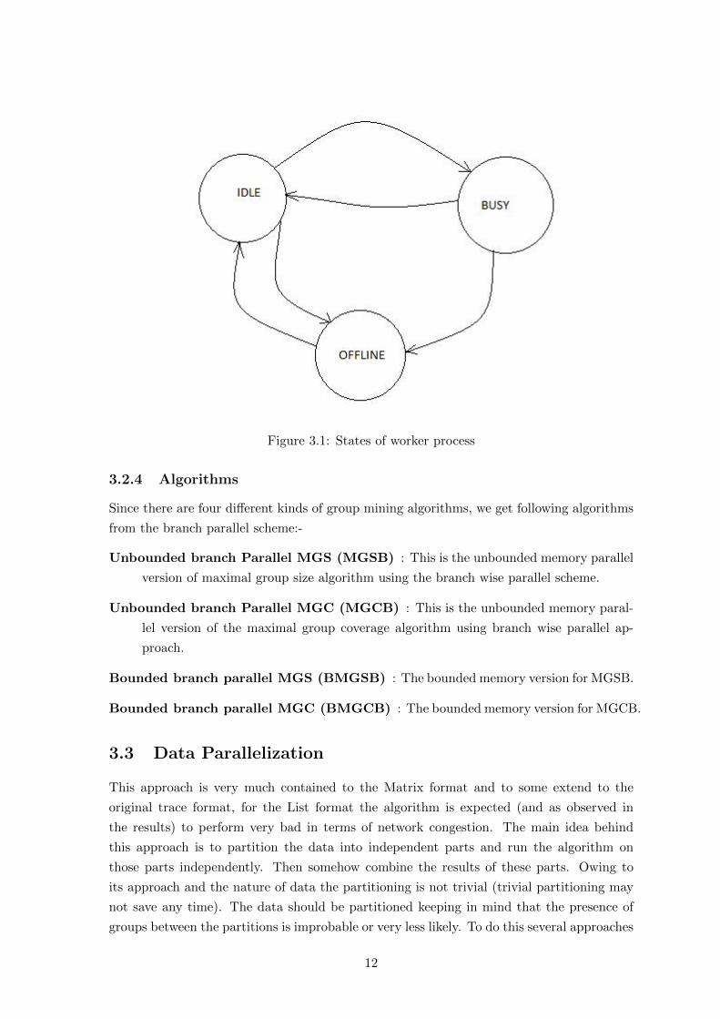
Figure 3.1: States of worker process

3.2.4 Algorithms

Since there are four different kinds of group mining algorithms, we get following algorithms

from the branch parallel scheme:-

Unbounded branch Parallel MGS (MGSB) : This is the unbounded memory parallel

version of maximal group size algorithm using the branch wise parallel scheme.

Unbounded branch Parallel MGC (MGCB) : This is the unbounded memory paral-

lel version of the maximal group coverage algorithm using branch wise parallel ap-

proach.

Bounded branch parallel MGS (BMGSB) : The bounded memory version for MGSB.

Bounded branch parallel MGC (BMGCB) : The bounded memory version for MGCB.

3.3 Data Parallelization

This approach is very much contained to the Matrix format and to some extend to the

original trace format, for the List format the algorithm is expected (and as observed in

the results) to perform very bad in terms of network congestion. The main idea behind

this approach is to partition the data into independent parts and run the algorithm on

those parts independently. Then somehow combine the results of these parts. Owing to

its approach and the nature of data the partitioning is not trivial (trivial partitioning may

not save any time). The data should be partitioned keeping in mind that the presence of

groups between the partitions is improbable or very less likely. To do this several approaches

12

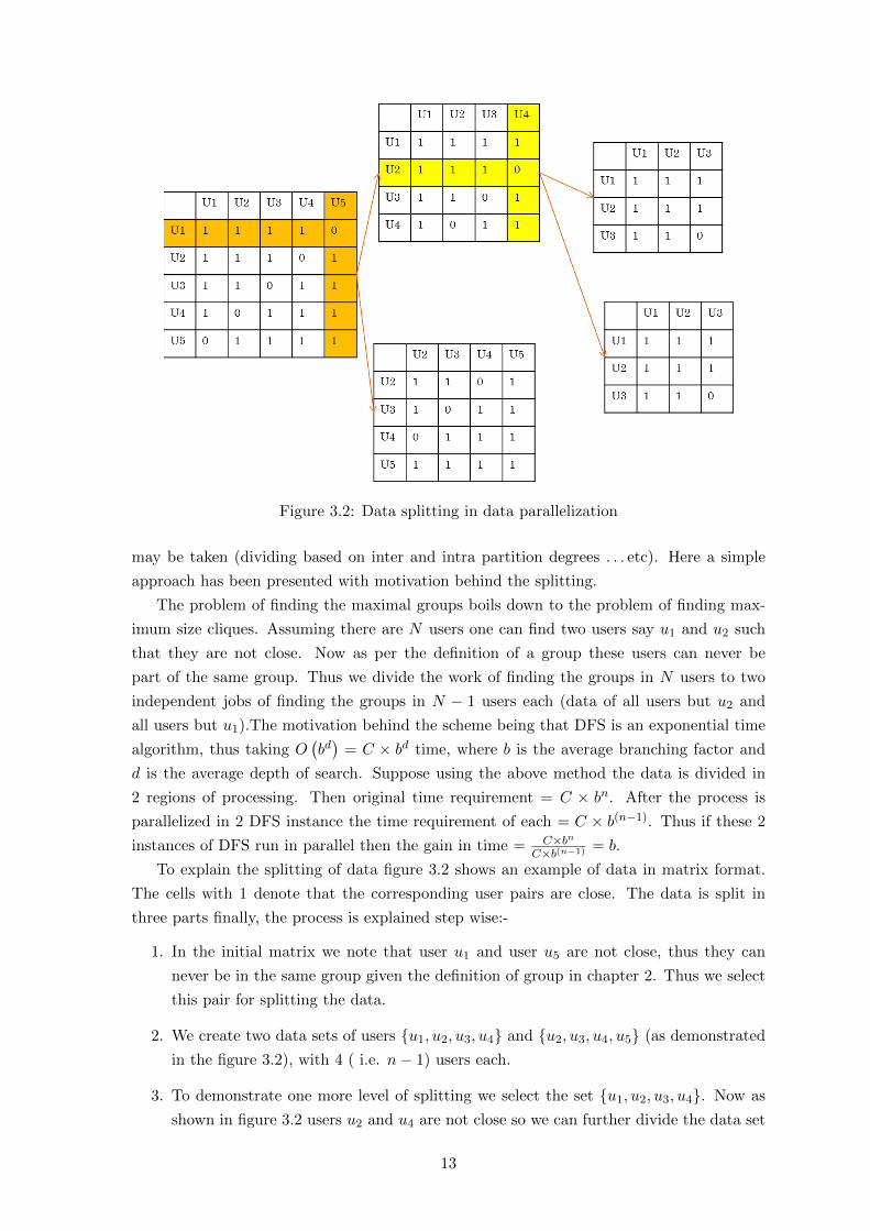
Figure 3.2: Data splitting in data parallelization

may be taken (dividing based on inter and intra partition degrees . . . etc). Here a simple

approach has been presented with motivation behind the splitting.

The problem of finding the maximal groups boils down to the problem of finding max-

imum size cliques. Assuming there are N users one can find two users say u1 and u2 such

that they are not close. Now as per the definition of a group these users can never be

part of the same group. Thus we divide the work of finding the groups in N users to two

independent jobs of finding the groups in N − 1 users each (data of all users but u2 and

all users but u1).The motivation behind the scheme being that DFS is an exponential time

algorithm, thus taking O(bd)

= C × bd time, where b is the average branching factor and

d is the average depth of search. Suppose using the above method the data is divided in

2 regions of processing. Then original time requirement = C × bn. After the process is

parallelized in 2 DFS instance the time requirement of each = C × b(n−1). Thus if these 2

instances of DFS run in parallel then the gain in time = C×bn

C×b(n−1) = b.

To explain the splitting of data figure 3.2 shows an example of data in matrix format.

The cells with 1 denote that the corresponding user pairs are close. The data is split in

three parts finally, the process is explained step wise:-

1. In the initial matrix we note that user u1 and user u5 are not close, thus they can

never be in the same group given the definition of group in chapter 2. Thus we select

this pair for splitting the data.

2. We create two data sets of users {u1, u2, u3, u4} and {u2, u3, u4, u5} (as demonstrated

in the figure 3.2), with 4 ( i.e. n− 1) users each.

3. To demonstrate one more level of splitting we select the set {u1, u2, u3, u4}. Now as

shown in figure 3.2 users u2 and u4 are not close so we can further divide the data set

13

in two set: {u1, u2, u3} and {u1, u3, u4} as shown in the figure.

4. Thus after 2 splittings we have three sets:-{u2, u3, u4, u5},{u1, u3, u4} and {u1, u2, u3}.

For a data set of 1000 users the average branching factor can be huge, thus one can

expect to gain lot of time even if the number of partitions are less.

The Organization of the approach is same as that detailed for the branch-wise paral-

lelization with Master and worker processes. The division of data is a recursive process of

finding two users in a set which can’t form a group. The approach is expected to work best

on sparse Matrices (which is actually the case here). Here also the intermediate results of

one worker can be used with other processes by implementing a distributed hash table. The

main advantage of using this approach is that since the processes use property of data for

parallelization the speedup is expected to be high. The degree of parallelization is subject

to the data.

3.3.1 Algorithms

Since there are four different kinds of group mining algorithms, we get following algorithms

from the branch parallel scheme:-

Unbounded branch Parallel MGS (MGSD) : This is the unbounded memory parallel

version of maximal group size algorithm using the data parallel scheme.

Unbounded branch Parallel MGC (MGCD) : This is the unbounded memory paral-

lel version of the maximal group coverage algorithm using data parallel approach.

Bounded branch parallel MGS (BMGSD) : The bounded memory version for MGSD.

Bounded branch parallel MGC (BMGCD) : The bounded memory version for MGCD.

3.4 Memory Bounded Versions

For the memory bounded version the size of the open and closed list is fixed in all the nodes

of the cluster (except the master node). In Memory bounded versions the algorithms are

breadth first rather than depth first, thus there need to be some modifications in the branch

wise parallelization technique (the data-parallelization technique can be used as it is).

3.4.1 Modification in Branch Parallelization

Since the underlying algorithm has become A∗, now each worker has an open and closed

lists (sum of sizes of these two are bounded). In this modified design the worker executes

the A∗ algorithm to a certain depth (just like in the unmodified version), but instead of

assigning a particular node from the open list to a worker, the master partitions the open

list into the required number of partitions (= number of cluster nodes). Then each partition

is sent to a worker which then resumes the MAWA∗ [10] algorithm from that point on with

closed list initialized to empty list. After a particular time step, say T seconds (= 5sec

in the implementation), the master requests the workers to report their “anytime” best

14

solutions along with the open lists. The Master on receiving these lists and the solutions

updates the local solutions (if needed) and computes the union of all the open lists. Then

the unified open list is repartitioned into the cluster nodes, which carry on the execution of

the MAWA∗ algorithm.

The major modification witnessed in this algorithm is the periodic requests from master

to resynchronize the workers because without this step it was witnessed that the speedup

was negligible. This modification not only redistributes the work on slaves from time to

time but also reduces the number of times a node is explored in the distributed running of

MAWA∗.

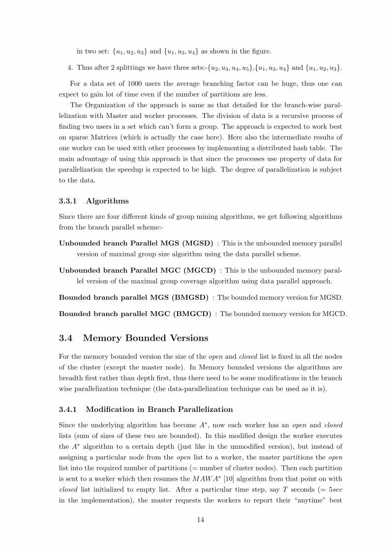
3.4.2 Selecting Optimal Value of T

In this section we analyze the effect of T on the performance of the above mentioned

algorithm for a dataset of 1000 users. All the figures are estimated over 5 runs, with

number of workers = 20.

Figure 3.3: Speedup vs T

In Figure 3.3 Y -axis denotes the speedup of the parallel version over the sequential

version, and the X-axis denotes the values of T. It can be seen from the graph that the

speedup initially increases to around 6 for T = 5sec and then rapidly falls back. It can be

explained by the fact that when the values of T are small most of the time is spent by the

workers communicating with the master (as depicted by the CPU load on master in the

table below). After T = 5 the speedup decreases because the time window becomes too

wide to avoid re-exploration of a node in the A∗ algorithm. Table 3.1 shows the variation of

CPU load on the master with change in values of T . From the table it can be conclusively

said that the modification does not incur a lot of overhead in terms of load on master, thus

scalability issues do not arise from the side of master.

15

Value of T (in sec) CPU load on master (terms of a single CPU time)

0.01 1.23

0.05 0.98

1 0.67

2 0.4

3 0.3

4 0.10

5 0.10

Table 3.1: Load on master with T

3.5 Design issues

For the parallelization we take several approaches to utilize the complete computation re-

sources. While parallelization of an algorithm that operates on a vast data set, the space

requirement of the algorithm also forms an important metric for qualitative evaluation along

with the time saved by the approach. In this section we present the factors that account

for the feasibility of a distributed computing approach for an algorithm. All the approaches

are then presented in the following sections while showing their evaluation on these factors.

3.5.1 Time Requirements

The time required by an algorithm is one of the most obvious and noticeable factor for

choosing a parallelization approach. The amount of speedup achieved in a parallel algorithm

should ideally be equal to the number of free machines available in a cluster; however in

most cases this level of improvement is not possible either because the problem can’t be

parallelized to an arbitrary degree or due to the communications between different pieces

of code.

3.5.2 Data Storage Requirements

Data Placement The amount of storage required and the time advantage for a partic-

ular distributed computing approach often act as trade offs. For example assume a data

distribution approach where each machine in the cluster has a local copy of the dataset.

The execution speed will definitely be faster than the case where the data is shared us-

ing some distributed file system (as the former approach reduces the network overheads of

data access). However in the former case the amount of storage capacity required shall be

huge, increasing linearly with the number of machines used. Whereas in the second case

the amount of storage required is (almost) constant with respect to the number of machines

in the cluster, resulting in scalable architecture but requiring a lot more time due to the

network delays that come into play while accessing the shared data. Not only time, the

data storage used also dictates the network congestion in the system.

Data Format Here we show the analysis for the storage requirements of the different data

organizations discussed above. Figure 3.5.2 shows the variation in the size requirements of

various data formats as the number of users increase in the trace. It can be seen that the

16

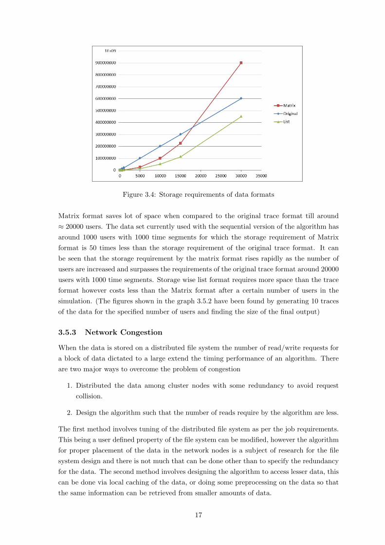
Figure 3.4: Storage requirements of data formats

Matrix format saves lot of space when compared to the original trace format till around

≈ 20000 users. The data set currently used with the sequential version of the algorithm has

around 1000 users with 1000 time segments for which the storage requirement of Matrix

format is 50 times less than the storage requirement of the original trace format. It can

be seen that the storage requirement by the matrix format rises rapidly as the number of

users are increased and surpasses the requirements of the original trace format around 20000

users with 1000 time segments. Storage wise list format requires more space than the trace

format however costs less than the Matrix format after a certain number of users in the

simulation. (The figures shown in the graph 3.5.2 have been found by generating 10 traces

of the data for the specified number of users and finding the size of the final output)

3.5.3 Network Congestion

When the data is stored on a distributed file system the number of read/write requests for

a block of data dictated to a large extend the timing performance of an algorithm. There

are two major ways to overcome the problem of congestion

1. Distributed the data among cluster nodes with some redundancy to avoid request

collision.

2. Design the algorithm such that the number of reads require by the algorithm are less.

The first method involves tuning of the distributed file system as per the job requirements.

This being a user defined property of the file system can be modified, however the algorithm

for proper placement of the data in the network nodes is a subject of research for the file

system design and there is not much that can be done other than to specify the redundancy

for the data. The second method involves designing the algorithm to access lesser data, this

can be done via local caching of the data, or doing some preprocessing on the data so that

the same information can be retrieved from smaller amounts of data.

17

Chapter 4

Results

The algorithms discussed above have been implemented in python with use of the aima-

python open source package. Hadoop is used as the distributed file system for executing the

pre-processing tasks of Map-reduce as well as for providing a space efficient high performance

central file serving system for the workers. The Hadoop cluster on which this implementation

was run consisted of only 20 nodes, however the code can be made to scale to higher number

of machine nodes with minor changes. The results have been divided in two parts

Simulations In this part of algorithm analysis the user mobility trace was artificially gen-

erated using a mobility model. We call this the results with dataset 1.

Actual Traces In this part of algorithm analysis the user mobility data is collected from

actual human mobility in a well defined area. We call this the results with dataset 2.

The rest of this chapter is organized in sections, in section 4.1 we briefly describe the

data used for the experiments while giving some analysis on the nature of data. Following

this, in section 4.2 we explain the preprocessing required for the data obtained. This is

followed by the results for dataset 1 on MGS (section 4.3) and MGC (section 4.4), and then

results on dataset 2 on MGS (section 4.6) and MGC (section 4.7). Section 4.9 presents a

brief analysis on the tunable parameters of the algorithm and finally section 4.10 presents

an outline conclusion from the experimetal results.

4.1 Datasets

In this section we describe the datasets used in the experiments and how they were obtained.

For the real user dataset we also provide some results

4.1.1 Artificial Data: dataset 1

We consider a random walk based location time simulator to generate the artificial trace

data. The details of the data are:

• Space: base grid of size 1000× 1000 square units

• Starting location: Generated randomly for each user on the above mentioned grid.

18

• Motion: At each time segment a user stays at its previous location with a probability

of 0.5. If it decides to move, it moves with equal probability in four directions.

The above parameters can be further tuned to get a much more realistic data. Since the

above mentioned model is a well studied random-walk variant, we omit analysis of the

VG-graph formed in this case

4.1.2 Dartmouth Data: dataset 2

Overview

The results presented in this section are obtained from actual mobility pattern [6] made

available by CRAWDAD (Community Resource for Archiving Wireless Data At Dartmouth)

at Dartmouth. The Mobility data is collected configuring the WiFi access points to send a

sys-log to a main server periodically where the sys-log consists of Wifi access events like a

users authenticating, Attaching, detaching, re-attaching . . . etc. Given this syslog and the

arrangement of Wifi access points over the campus a parser program [5] can generate a

mobility trace of the users.

The users are distinguished by the MAC addresses of the network interface card they

are using. The dataset [6] used in the current experiments is a very large data base collected

over 4 years from 2001 to 2004 with as much as 25000 unique MAC addresses in the system

logs.

Analysis

Since the Dartmouth data is not exactly a user mobility trace the definition of closeness

needs to be changed. Only in this section of discussion for the sake of simplicity the closeness

between two users is defined with respect to the time these users spend associated with same

wifi points. Thus if two users u1 and u2 spend a threshold amount of time connected to

same WiFi access points then these users are said to be close. Since the mobility data is

collected over 4-years the results presented herein are an average over results obtained for

the four years separately.

Close Pairs

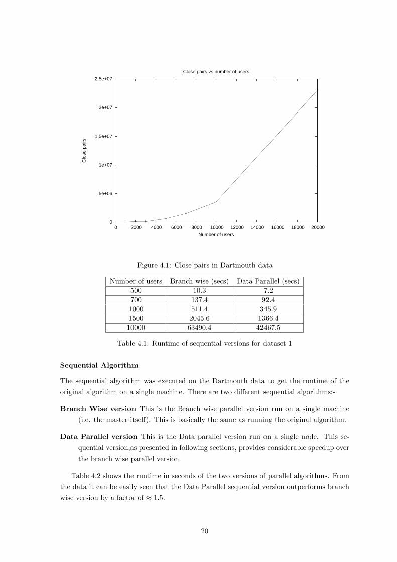
Figure 4.1 shows the graph of close pairs in the system log as the number of users considered

in the trace are increased. It can be seen that the number of close pairs increase in the same

trend throughout the range of 1000 to 20000 users. Thus the entire range is suitable for

running the group mining algorithms. It can also be seen that the number of close pairs

denote that the VG-graph formed for the user mobility in Dartmouth is a dense graph as

the number of close pairs show quadratic increase with increase in number of users.

Table 4.1 shows the execution time of the sequential algorithm on the dataset 1 for the

branch parallel and data parallel schemes. These results shall be used as a base line to

compare the speedup of the schemes in the following sections.

19

0

5e+06

1e+07

1.5e+07

2e+07

2.5e+07

0 2000 4000 6000 8000 10000 12000 14000 16000 18000 20000

Clo

se p

airs

Number of users

Close pairs vs number of users

Figure 4.1: Close pairs in Dartmouth data

Number of users Branch wise (secs) Data Parallel (secs)

500 10.3 7.2

700 137.4 92.4

1000 511.4 345.9

1500 2045.6 1366.4

10000 63490.4 42467.5

Table 4.1: Runtime of sequential versions for dataset 1

Sequential Algorithm

The sequential algorithm was executed on the Dartmouth data to get the runtime of the

original algorithm on a single machine. There are two different sequential algorithms:-

Branch Wise version This is the Branch wise parallel version run on a single machine

(i.e. the master itself). This is basically the same as running the original algorithm.

Data Parallel version This is the Data parallel version run on a single node. This se-

quential version,as presented in following sections, provides considerable speedup over

the branch wise parallel version.

Table 4.2 shows the runtime in seconds of the two versions of parallel algorithms. From

the data it can be easily seen that the Data Parallel sequential version outperforms branch

wise version by a factor of ≈ 1.5.

20

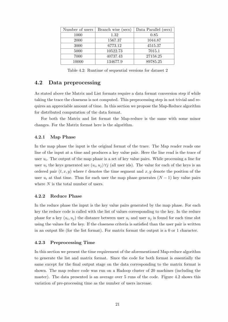
Number of users Branch wise (secs) Data Parallel (secs)

1000 1.32 0.85

2000 1567.37 1044.87

3000 6773.12 4515.37

5000 10522.73 7015.1

7000 40737.43 27158.25

10000 134677.9 89785.25

Table 4.2: Runtime of sequential versions for dataset 2

4.2 Data preprocessing

As stated above the Matrix and List formats require a data format conversion step if while

taking the trace the closeness is not computed. This preprocessing step in not trivial and re-

quires an appreciable amount of time. In this section we propose the Map-Reduce algorithm

for distributed computation of the data format.

For both the Matrix and list format the Map-reduce is the same with some minor

changes. For the Matrix format here is the algorithm.

4.2.1 Map Phase

In the map phase the input is the original format of the trace. The Map reader reads one

line of the input at a time and produces a key value pair. Here the line read is the trace of

user ui. The output of the map phase is a set of key value pairs. While processing a line for

user ui the keys generated are (ui, uj) ∀j (all user ids). The value for each of the keys is an

ordered pair (t, x, y) where t denotes the time segment and x, y denote the position of the

user ui at that time. Thus for each user the map phase generates (N − 1) key value pairs

where N is the total number of users.

4.2.2 Reduce Phase

In the reduce phase the input is the key value pairs generated by the map phase. For each

key the reduce code is called with the list of values corresponding to the key. In the reduce

phase for a key (ui, uj) the distance between user ui and user uj is found for each time slot

using the values for the key. If the closeness criteria is satisfied than the user pair is written

in an output file (for the list format). For matrix format the output is a 0 or 1 character.

4.2.3 Preprocessing Time

In this section we present the time requirement of the aforementioned Map-reduce algorithm

to generate the list and matrix format. Since the code for both format is essentially the

same except for the final output stage on the data corresponding to the matrix format is

shown. The map reduce code was run on a Hadoop cluster of 20 machines (including the

master). The data presented is an average over 5 runs of the code. Figure 4.2 shows this

variation of pre-processing time as the number of users increase.

21

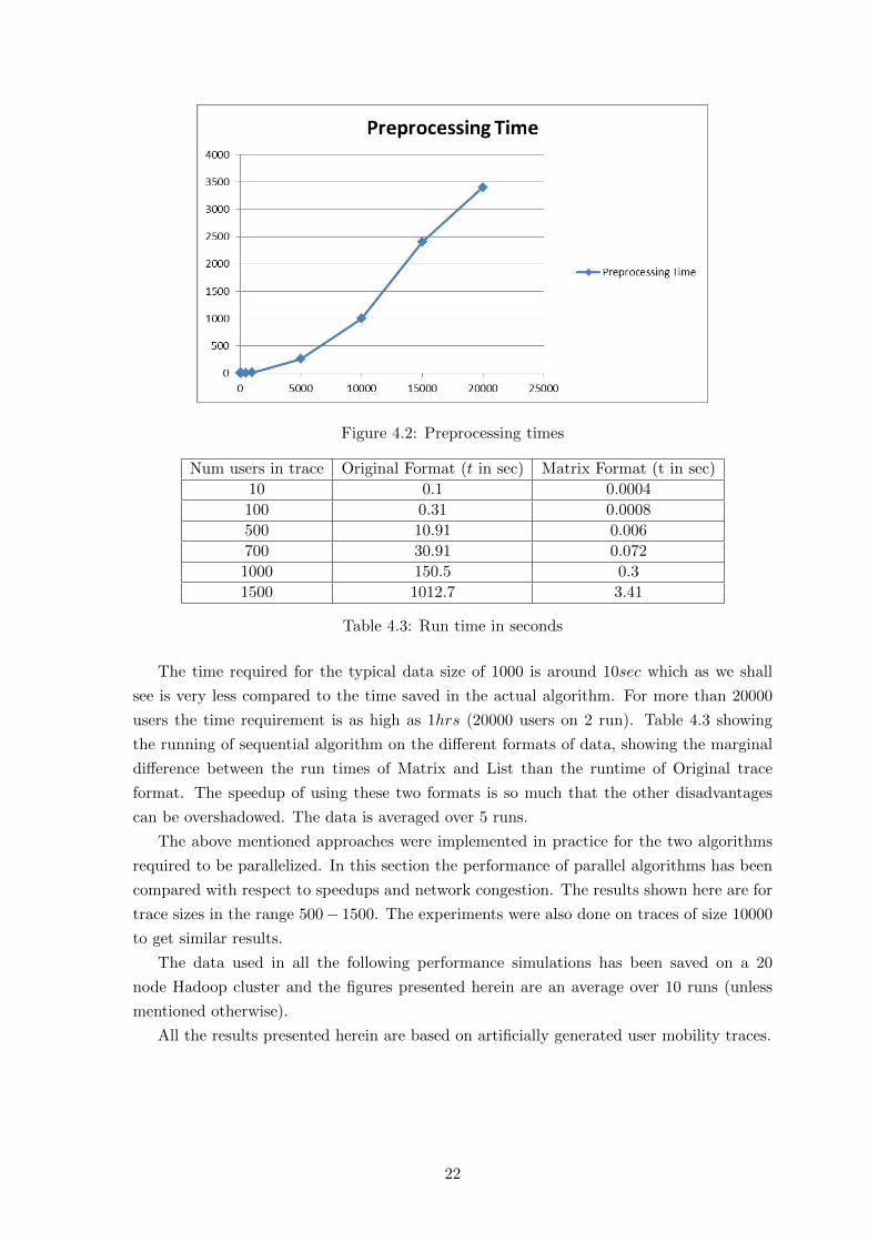
Figure 4.2: Preprocessing times

Num users in trace Original Format (t in sec) Matrix Format (t in sec)

10 0.1 0.0004

100 0.31 0.0008

500 10.91 0.006

700 30.91 0.072

1000 150.5 0.3

1500 1012.7 3.41

Table 4.3: Run time in seconds

The time required for the typical data size of 1000 is around 10sec which as we shall

see is very less compared to the time saved in the actual algorithm. For more than 20000

users the time requirement is as high as 1hrs (20000 users on 2 run). Table 4.3 showing

the running of sequential algorithm on the different formats of data, showing the marginal

difference between the run times of Matrix and List than the runtime of Original trace

format. The speedup of using these two formats is so much that the other disadvantages

can be overshadowed. The data is averaged over 5 runs.

The above mentioned approaches were implemented in practice for the two algorithms

required to be parallelized. In this section the performance of parallel algorithms has been

compared with respect to speedups and network congestion. The results shown here are for

trace sizes in the range 500− 1500. The experiments were also done on traces of size 10000

to get similar results.

The data used in all the following performance simulations has been saved on a 20

node Hadoop cluster and the figures presented herein are an average over 10 runs (unless

mentioned otherwise).

All the results presented herein are based on artificially generated user mobility traces.

22

4.3 Parallel MGS with dataset 1

In this section we present the performance of the parallelization approaches on finding the

maximal K groups in the trace. Since the Original trace format performs very poorly as

discussed above it has been omitted in certain graphs (to make the graphs visually better).

4.3.1 Unbounded Memory

Branch Parallelization MGSB The graphs in figure 4.3.1 point out the speedups

achieved using the parallel version of the DFS algorithm. The Different values of R de-

note the redundancy ratio used in the file system. By comparing the values at different

redundancy ratios one can comment on the network congestion caused by the algorithm.

The X-axis denotes the number of users in the trace and the Y -axis denotes the speedup

against the sequential version running on the same data format.

17.2

17.4

17.6

17.8

18

18.2

18.4

18.6

18.8

19

19.2

400 600 800 1000 1200 1400 1600

Spe

edup

Number of Users

R=1R=2R=3

(a) Matrix Format

15

15.5

16

16.5

17

17.5

18

18.5

19

19.5

400 600 800 1000 1200 1400 1600

Spe

edup

Number of Users

R=1R=2R=3

(b) List Format

Figure 4.3: Speedup of MGSB

The two graphs in figure 4.3(a) and 4.3(b) clearly show the speedups achieved depend

on the redundancy ratio, thus indicating that the algorithm performance is compromised

by congestion in the traffic. One can notice that the change in the curve with increase in

the redundancy ratio is more in the case of the list format, signifying that the algorithm

suffered more congestion in the case of data stores as a list than the case when data is stored

as a matrix.

Load on master The graph shown in figure 4.4 clearly depicts the load on a Master

Process in terms of CPU utilization (averaged) over the entire runtime (taking samples at

regular intervals of 10 sec) with variation in the number of worker processes. The graph

depicts that the load on master gradually increases with the increase in workers and shows

an almost linear trend (the figures are taken for a data set of 1000 users). The graph also

suggests that the algorithm cannot be scaled to very large cluster (more than 100s of nodes)

without distributing the work of master itself.

23

0.12

0.14

0.16

0.18

0.2

0.22

0.24

0.26

0.28

0.3

2 4 6 8 10 12 14 16 18 20

CP

U L

oad

Number of Workers

CPU load vs number of workers

Load

Figure 4.4: Master load in MGSB

Data Parallel version MGSD The graphs shown in figure 4.3.1 point out the speedups

achieved using the partitioning of data. The Different values of R denote the redundancy

ratio used in the file system. By comparing the values at different redundancy ratios one

can comment on the network congestion caused by the algorithm. The X-axis denotes the

number of users in the trace and the Y -axis denotes the speedup against the sequential

version running on the same data format.

18

18.2

18.4

18.6

18.8

19

19.2

400 600 800 1000 1200 1400 1600

Spe

edup

Number of Users

R=1R=2R=3

(a) Matrix Format

17.4

17.6

17.8

18

18.2

18.4

18.6

18.8

19

19.2

400 600 800 1000 1200 1400 1600

Spe

edup

Number of Users

R=1R=2R=3

(b) List Format

Figure 4.5: Speedup of MGSD

Graphs in figure 4.5(a) and 4.5(b) also suggest that speedups can be achieved in using

partitioning of data. An important point to be noted is that the sequential version of data

parallel algorithm is ≈ 1.5 times faster than that of the branch parallel version, thus as

compared to that the speedup will be greater than 20, the number of workers in the clus-

ter.Again the graph for List format shows greater variation in the speedups which increase

in the redundancy ratio depicting that list format is more susceptible to congestions.

24

0.13

0.135

0.14

0.145

0.15

0.155

0.16

0.165

0.17

0.175

0.18

2 4 6 8 10 12 14 16 18 20

CP

U L

oad

Number of Workers

CPU load vs number of workers

Load

Figure 4.6: Master load in MGSD

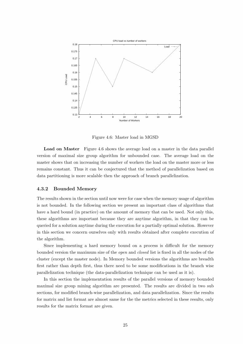
Load on Master Figure 4.6 shows the average load on a master in the data parallel

version of maximal size group algorithm for unbounded case. The average load on the

master shows that on increasing the number of workers the load on the master more or less

remains constant. Thus it can be conjectured that the method of parallelization based on

data partitioning is more scalable then the approach of branch parallelization.

4.3.2 Bounded Memory

The results shown in the section until now were for case when the memory usage of algorithm

is not bounded. In the following section we present an important class of algorithms that

have a hard bound (in practice) on the amount of memory that can be used. Not only this,

these algorithms are important because they are anytime algorithm, in that they can be

queried for a solution anytime during the execution for a partially optimal solution. However

in this section we concern ourselves only with results obtained after complete execution of

the algorithm.

Since implementing a hard memory bound on a process is difficult for the memory

bounded version the maximum size of the open and closed list is fixed in all the nodes of the

cluster (except the master node). In Memory bounded versions the algorithms are breadth

first rather than depth first, thus there need to be some modifications in the branch wise

parallelization technique (the data-parallelization technique can be used as it is).

In this section the implementation results of the parallel versions of memory bounded

maximal size group mining algorithm are presented. The results are divided in two sub

sections, for modified branch-wise parallelization, and data parallelization. Since the results

for matrix and list format are almost same for the the metrics selected in these results, only

results for the matrix format are given.

25

5.7

5.75

5.8

5.85

5.9

400 600 800 1000 1200 1400 1600

Spe

edup

Number of Users

MatrixList

Figure 4.7: Speedup for BMGSB with matrix format

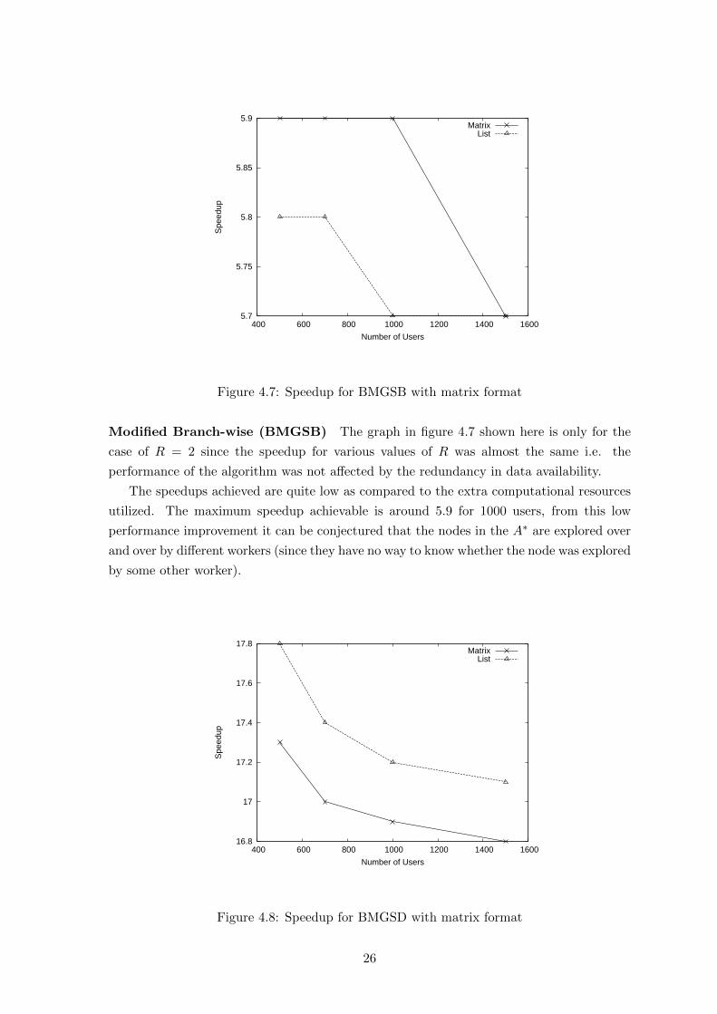
Modified Branch-wise (BMGSB) The graph in figure 4.7 shown here is only for the

case of R = 2 since the speedup for various values of R was almost the same i.e. the

performance of the algorithm was not affected by the redundancy in data availability.

The speedups achieved are quite low as compared to the extra computational resources

utilized. The maximum speedup achievable is around 5.9 for 1000 users, from this low

performance improvement it can be conjectured that the nodes in the A∗ are explored over

and over by different workers (since they have no way to know whether the node was explored

by some other worker).

16.8

17

17.2

17.4

17.6

17.8

400 600 800 1000 1200 1400 1600

Spe

edup

Number of Users

MatrixList

Figure 4.8: Speedup for BMGSD with matrix format

26

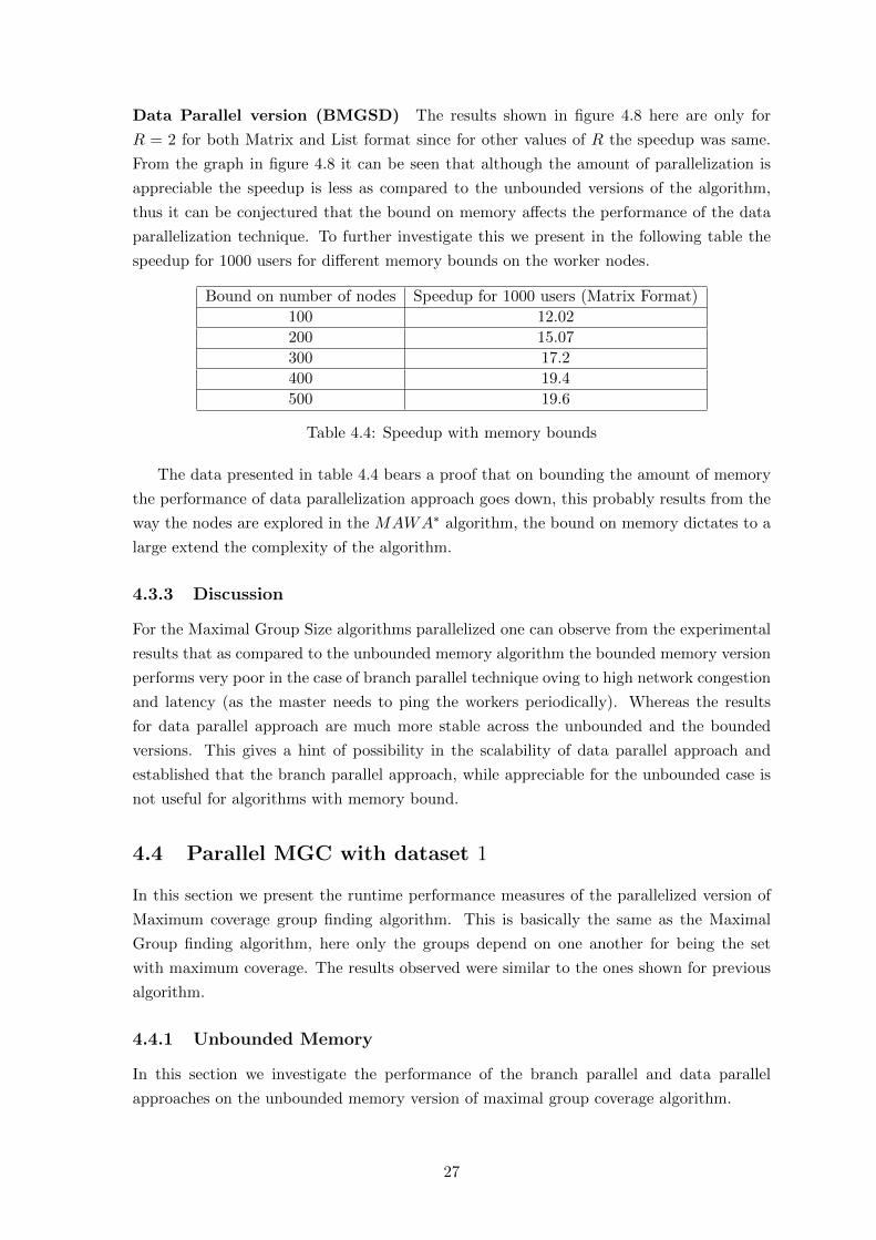
Data Parallel version (BMGSD) The results shown in figure 4.8 here are only for

R = 2 for both Matrix and List format since for other values of R the speedup was same.

From the graph in figure 4.8 it can be seen that although the amount of parallelization is

appreciable the speedup is less as compared to the unbounded versions of the algorithm,

thus it can be conjectured that the bound on memory affects the performance of the data

parallelization technique. To further investigate this we present in the following table the

speedup for 1000 users for different memory bounds on the worker nodes.

Bound on number of nodes Speedup for 1000 users (Matrix Format)

100 12.02

200 15.07

300 17.2

400 19.4

500 19.6

Table 4.4: Speedup with memory bounds

The data presented in table 4.4 bears a proof that on bounding the amount of memory

the performance of data parallelization approach goes down, this probably results from the

way the nodes are explored in the MAWA∗ algorithm, the bound on memory dictates to a

large extend the complexity of the algorithm.

4.3.3 Discussion

For the Maximal Group Size algorithms parallelized one can observe from the experimental

results that as compared to the unbounded memory algorithm the bounded memory version

performs very poor in the case of branch parallel technique oving to high network congestion

and latency (as the master needs to ping the workers periodically). Whereas the results

for data parallel approach are much more stable across the unbounded and the bounded

versions. This gives a hint of possibility in the scalability of data parallel approach and

established that the branch parallel approach, while appreciable for the unbounded case is

not useful for algorithms with memory bound.

4.4 Parallel MGC with dataset 1

In this section we present the runtime performance measures of the parallelized version of

Maximum coverage group finding algorithm. This is basically the same as the Maximal

Group finding algorithm, here only the groups depend on one another for being the set

with maximum coverage. The results observed were similar to the ones shown for previous

algorithm.

4.4.1 Unbounded Memory

In this section we investigate the performance of the branch parallel and data parallel

approaches on the unbounded memory version of maximal group coverage algorithm.

27

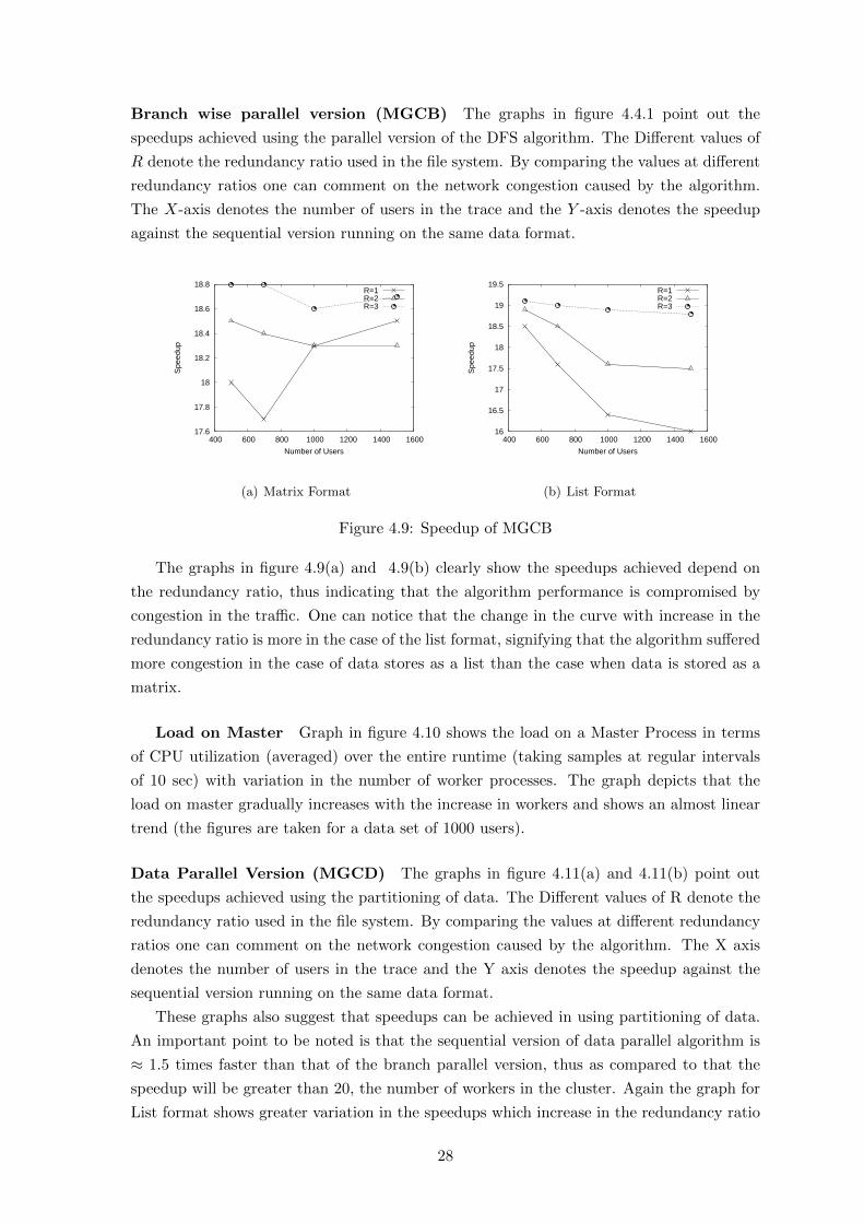
Branch wise parallel version (MGCB) The graphs in figure 4.4.1 point out the

speedups achieved using the parallel version of the DFS algorithm. The Different values of

R denote the redundancy ratio used in the file system. By comparing the values at different

redundancy ratios one can comment on the network congestion caused by the algorithm.

The X-axis denotes the number of users in the trace and the Y -axis denotes the speedup

against the sequential version running on the same data format.

17.6

17.8

18

18.2

18.4

18.6

18.8

400 600 800 1000 1200 1400 1600

Spe

edup

Number of Users

R=1R=2R=3

(a) Matrix Format

16

16.5

17

17.5

18

18.5

19

19.5

400 600 800 1000 1200 1400 1600

Spe

edup

Number of Users

R=1R=2R=3

(b) List Format

Figure 4.9: Speedup of MGCB

The graphs in figure 4.9(a) and 4.9(b) clearly show the speedups achieved depend on

the redundancy ratio, thus indicating that the algorithm performance is compromised by

congestion in the traffic. One can notice that the change in the curve with increase in the

redundancy ratio is more in the case of the list format, signifying that the algorithm suffered

more congestion in the case of data stores as a list than the case when data is stored as a

matrix.

Load on Master Graph in figure 4.10 shows the load on a Master Process in terms

of CPU utilization (averaged) over the entire runtime (taking samples at regular intervals

of 10 sec) with variation in the number of worker processes. The graph depicts that the

load on master gradually increases with the increase in workers and shows an almost linear

trend (the figures are taken for a data set of 1000 users).

Data Parallel Version (MGCD) The graphs in figure 4.11(a) and 4.11(b) point out

the speedups achieved using the partitioning of data. The Different values of R denote the

redundancy ratio used in the file system. By comparing the values at different redundancy

ratios one can comment on the network congestion caused by the algorithm. The X axis

denotes the number of users in the trace and the Y axis denotes the speedup against the

sequential version running on the same data format.

These graphs also suggest that speedups can be achieved in using partitioning of data.

An important point to be noted is that the sequential version of data parallel algorithm is

≈ 1.5 times faster than that of the branch parallel version, thus as compared to that the

speedup will be greater than 20, the number of workers in the cluster. Again the graph for

List format shows greater variation in the speedups which increase in the redundancy ratio

28

0.1

0.12

0.14

0.16

0.18

0.2

0.22

0.24

0.26

0.28

0.3

2 4 6 8 10 12 14 16 18 20

CP

U L

oad

Number of Workers

CPU load vs number of workers

Load

Figure 4.10: Master load in MGCB

17.6

17.8

18

18.2

18.4

18.6

18.8

19

400 600 800 1000 1200 1400 1600

Spe

edup

Number of Users

R=1R=2R=3

(a) Matrix Format

17.2

17.4

17.6

17.8

18

18.2

18.4

18.6

18.8

400 600 800 1000 1200 1400 1600

Spe

edup

Number of Users

R=1R=2R=3

(b) List Format

Figure 4.11: Speedup of MGCD

depicting that list format is more susceptible to congestions. However comparing the graph

to the corresponding graph for the Maximal groups algorithm we see that the variation in

list format is more in the case of Maximal Groups algorithm, thus depicting that the Data

partitioning algorithm encounters lesser traffic congestion for Maximum coverage algorithm

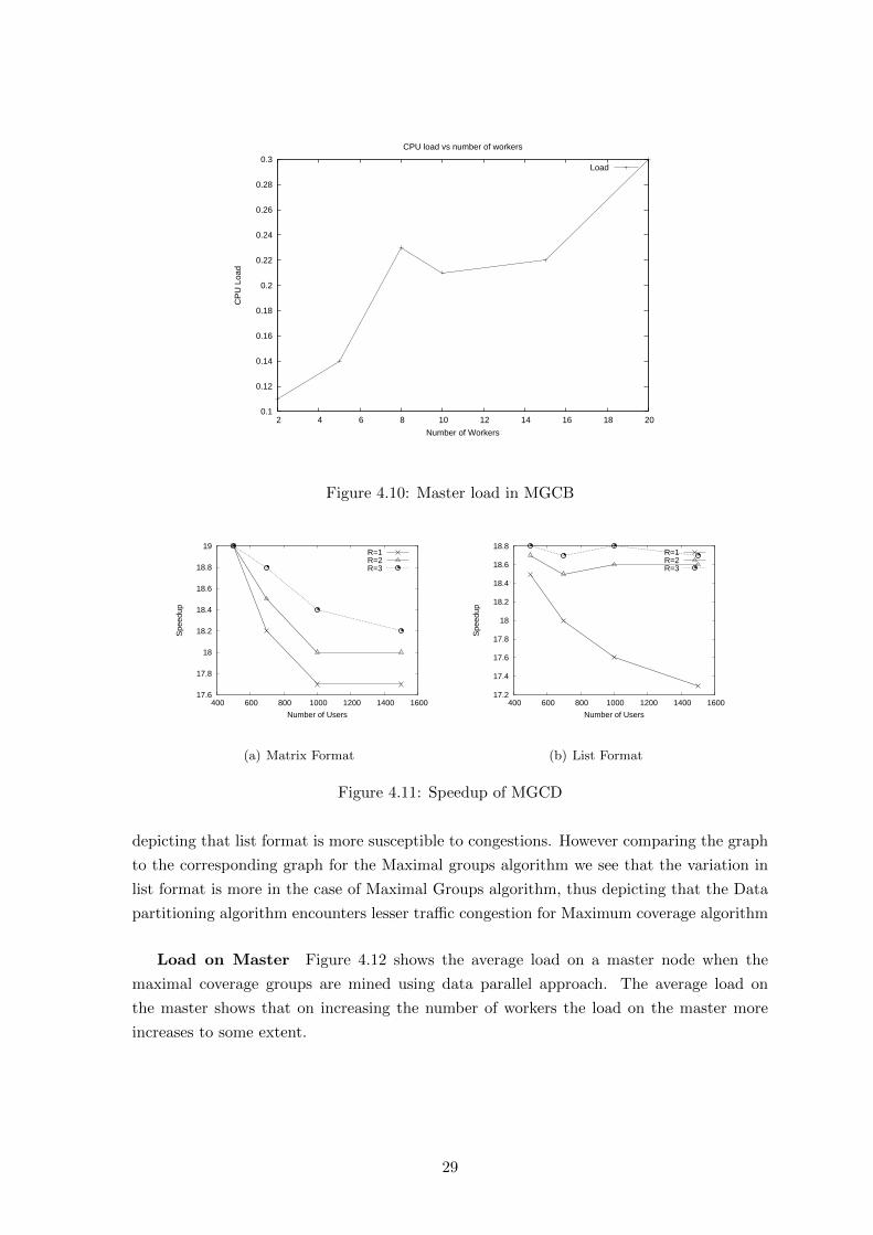
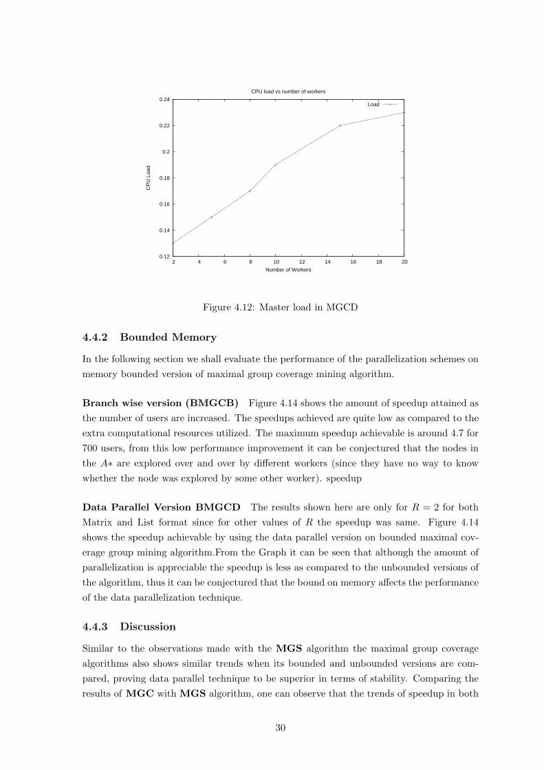
Load on Master Figure 4.12 shows the average load on a master node when the

maximal coverage groups are mined using data parallel approach. The average load on

the master shows that on increasing the number of workers the load on the master more

increases to some extent.

29

0.12

0.14

0.16

0.18

0.2

0.22

0.24

2 4 6 8 10 12 14 16 18 20

CP

U L

oad

Number of Workers

CPU load vs number of workers

Load

Figure 4.12: Master load in MGCD

4.4.2 Bounded Memory

In the following section we shall evaluate the performance of the parallelization schemes on

memory bounded version of maximal group coverage mining algorithm.

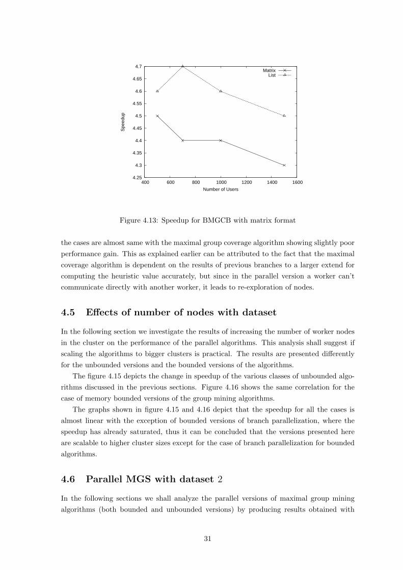
Branch wise version (BMGCB) Figure 4.14 shows the amount of speedup attained as

the number of users are increased. The speedups achieved are quite low as compared to the

extra computational resources utilized. The maximum speedup achievable is around 4.7 for

700 users, from this low performance improvement it can be conjectured that the nodes in

the A∗ are explored over and over by different workers (since they have no way to know

whether the node was explored by some other worker). speedup

Data Parallel Version BMGCD The results shown here are only for R = 2 for both

Matrix and List format since for other values of R the speedup was same. Figure 4.14

shows the speedup achievable by using the data parallel version on bounded maximal cov-

erage group mining algorithm.From the Graph it can be seen that although the amount of

parallelization is appreciable the speedup is less as compared to the unbounded versions of

the algorithm, thus it can be conjectured that the bound on memory affects the performance

of the data parallelization technique.

4.4.3 Discussion

Similar to the observations made with the MGS algorithm the maximal group coverage

algorithms also shows similar trends when its bounded and unbounded versions are com-

pared, proving data parallel technique to be superior in terms of stability. Comparing the

results of MGC with MGS algorithm, one can observe that the trends of speedup in both

30

4.25

4.3

4.35

4.4

4.45

4.5

4.55

4.6

4.65

4.7

400 600 800 1000 1200 1400 1600

Spe

edup

Number of Users

MatrixList

Figure 4.13: Speedup for BMGCB with matrix format

the cases are almost same with the maximal group coverage algorithm showing slightly poor

performance gain. This as explained earlier can be attributed to the fact that the maximal

coverage algorithm is dependent on the results of previous branches to a larger extend for

computing the heuristic value accurately, but since in the parallel version a worker can’t

communicate directly with another worker, it leads to re-exploration of nodes.

4.5 Effects of number of nodes with dataset

In the following section we investigate the results of increasing the number of worker nodes

in the cluster on the performance of the parallel algorithms. This analysis shall suggest if

scaling the algorithms to bigger clusters is practical. The results are presented differently

for the unbounded versions and the bounded versions of the algorithms.

The figure 4.15 depicts the change in speedup of the various classes of unbounded algo-

rithms discussed in the previous sections. Figure 4.16 shows the same correlation for the

case of memory bounded versions of the group mining algorithms.

The graphs shown in figure 4.15 and 4.16 depict that the speedup for all the cases is

almost linear with the exception of bounded versions of branch parallelization, where the

speedup has already saturated, thus it can be concluded that the versions presented here

are scalable to higher cluster sizes except for the case of branch parallelization for bounded

algorithms.

4.6 Parallel MGS with dataset 2

In the following sections we shall analyze the parallel versions of maximal group mining

algorithms (both bounded and unbounded versions) by producing results obtained with

31

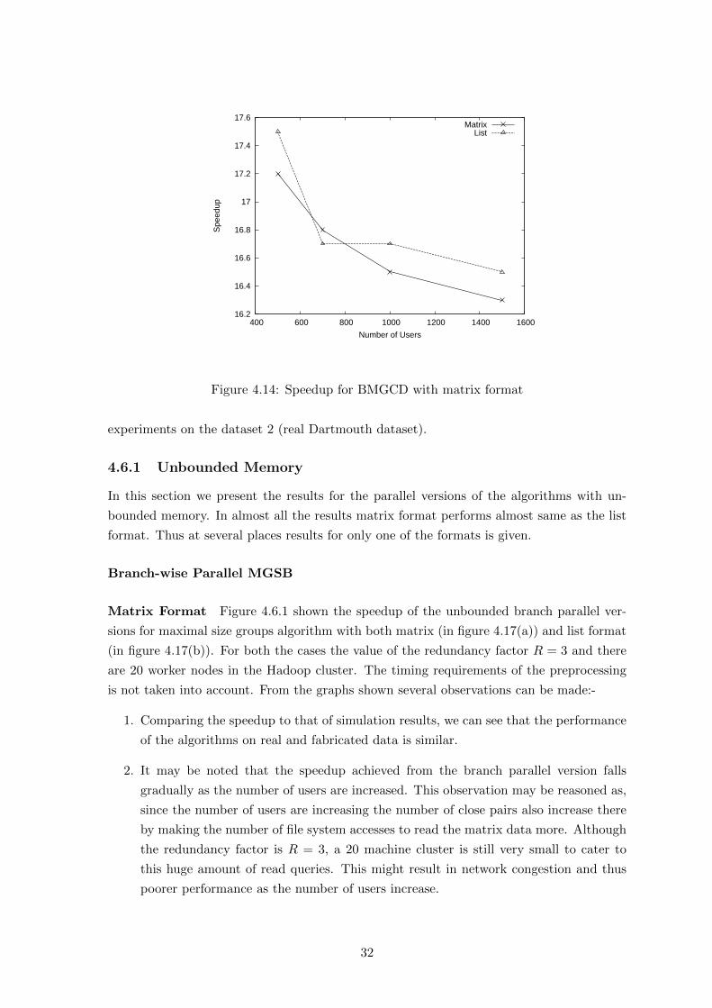
16.2

16.4

16.6

16.8

17

17.2

17.4

17.6

400 600 800 1000 1200 1400 1600

Spe

edup

Number of Users

MatrixList

Figure 4.14: Speedup for BMGCD with matrix format

experiments on the dataset 2 (real Dartmouth dataset).

4.6.1 Unbounded Memory

In this section we present the results for the parallel versions of the algorithms with un-

bounded memory. In almost all the results matrix format performs almost same as the list

format. Thus at several places results for only one of the formats is given.

Branch-wise Parallel MGSB

Matrix Format Figure 4.6.1 shown the speedup of the unbounded branch parallel ver-

sions for maximal size groups algorithm with both matrix (in figure 4.17(a)) and list format

(in figure 4.17(b)). For both the cases the value of the redundancy factor R = 3 and there

are 20 worker nodes in the Hadoop cluster. The timing requirements of the preprocessing

is not taken into account. From the graphs shown several observations can be made:-

1. Comparing the speedup to that of simulation results, we can see that the performance

of the algorithms on real and fabricated data is similar.

2. It may be noted that the speedup achieved from the branch parallel version falls

gradually as the number of users are increased. This observation may be reasoned as,

since the number of users are increasing the number of close pairs also increase there

by making the number of file system accesses to read the matrix data more. Although

the redundancy factor is R = 3, a 20 machine cluster is still very small to cater to

this huge amount of read queries. This might result in network congestion and thus

poorer performance as the number of users increase.

32

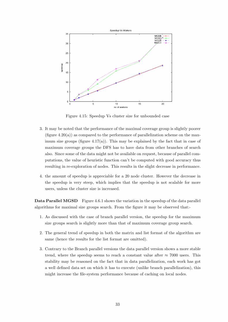
Figure 4.15: Speedup Vs cluster size for unbounded case

3. It may be noted that the performance of the maximal coverage group is slightly poorer

(figure 4.20(a)) as compared to the performance of parallelization scheme on the max-

imum size groups (figure 4.17(a)). This may be explained by the fact that in case of

maximum coverage groups the DFS has to have data from other branches of search

also. Since some of the data might not be available on request, because of parallel com-

putations, the value of heuristic function can’t be computed with good accuracy thus

resulting in re-exploration of nodes. This results in the slight decrease in performance.

4. the amount of speedup is appreciable for a 20 node cluster. However the decrease in

the speedup is very steep, which implies that the speedup is not scalable for more

users, unless the cluster size is increased.

Data Parallel MGSD Figure 4.6.1 shows the variation in the speedup of the data parallel

algorithms for maximal size groups search. From the figure it may be observed that:-

1. As discussed with the case of branch parallel version, the speedup for the maximum

size groups search is slightly more than that of maximum coverage group search.

2. The general trend of speedup in both the matrix and list format of the algorithm are

same (hence the results for the list format are omitted).

3. Contrary to the Branch parallel versions the data parallel version shows a more stable

trend, where the speedup seems to reach a constant value after ≈ 7000 users. This

stability may be reasoned on the fact that in data parallelization, each work has got

a well defined data set on which it has to execute (unlike branch parallelization), this

might increase the file-system performance because of caching on local nodes.

33

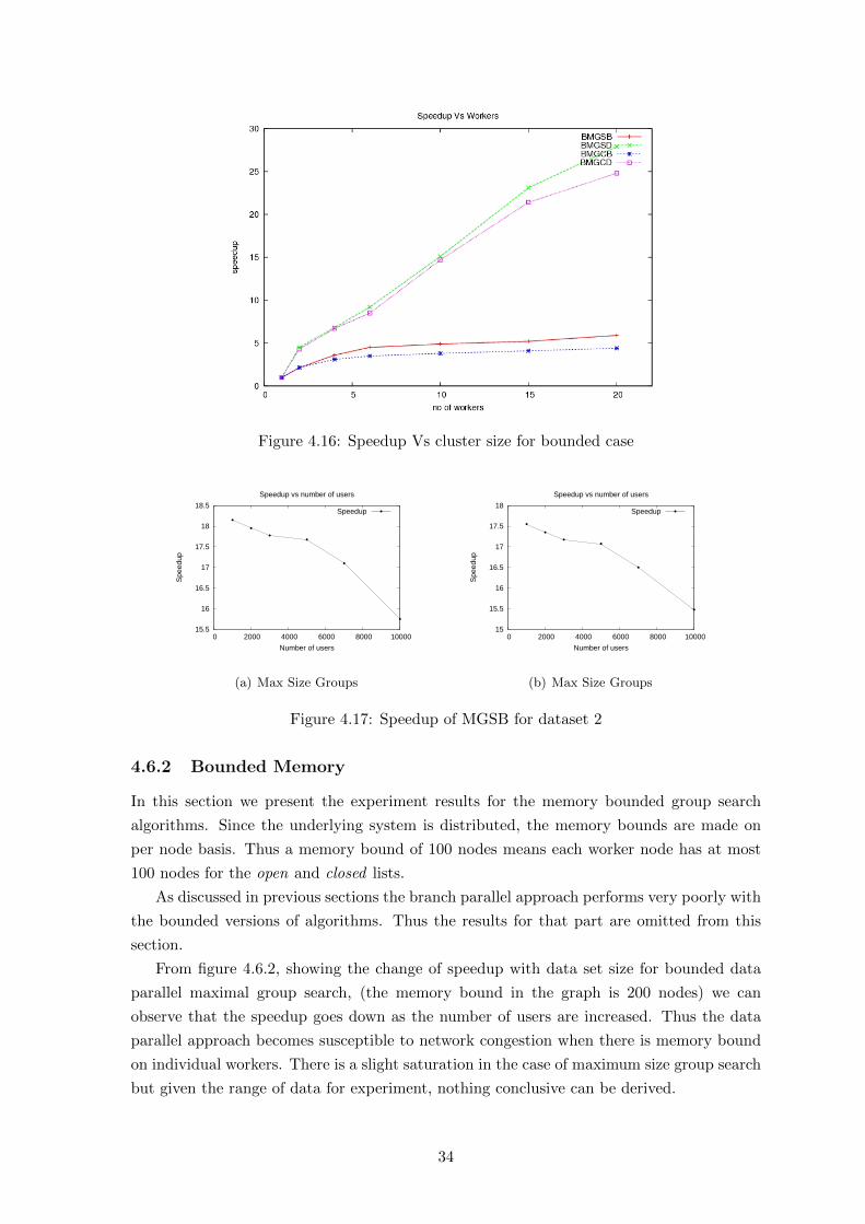
Figure 4.16: Speedup Vs cluster size for bounded case

15.5

16

16.5

17

17.5

18

18.5

0 2000 4000 6000 8000 10000

Spe

edup

Number of users

Speedup vs number of users

Speedup

(a) Max Size Groups

15

15.5

16

16.5

17

17.5

18

0 2000 4000 6000 8000 10000

Spe

edup

Number of users

Speedup vs number of users

Speedup

(b) Max Size Groups

Figure 4.17: Speedup of MGSB for dataset 2

4.6.2 Bounded Memory

In this section we present the experiment results for the memory bounded group search

algorithms. Since the underlying system is distributed, the memory bounds are made on

per node basis. Thus a memory bound of 100 nodes means each worker node has at most

100 nodes for the open and closed lists.

As discussed in previous sections the branch parallel approach performs very poorly with

the bounded versions of algorithms. Thus the results for that part are omitted from this

section.

From figure 4.6.2, showing the change of speedup with data set size for bounded data

parallel maximal group search, (the memory bound in the graph is 200 nodes) we can

observe that the speedup goes down as the number of users are increased. Thus the data

parallel approach becomes susceptible to network congestion when there is memory bound

on individual workers. There is a slight saturation in the case of maximum size group search

but given the range of data for experiment, nothing conclusive can be derived.

34

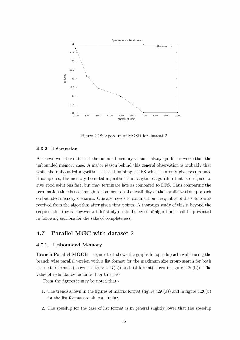
17

17.5

18

18.5

19

19.5

20

20.5

21

1000 2000 3000 4000 5000 6000 7000 8000 9000 10000

Spe

edup

Number of users

Speedup vs number of users

Speedup

Figure 4.18: Speedup of MGSD for dataset 2

4.6.3 Discussion

As shown with the dataset 1 the bounded memory versions always performs worse than the

unbounded memory case. A major reason behind this general observation is probably that

while the unbounded algorithm is based on simple DFS which can only give results once

it completes, the memory bounded algorithm is an anytime algorithm that is designed to

give good solutions fast, but may terminate late as compared to DFS. Thus comparing the

termination time is not enough to comment on the feasibility of the parallelization approach

on bounded memory scenarios. One also needs to comment on the quality of the solution as

received from the algorithm after given time points. A thorough study of this is beyond the

scope of this thesis, however a brief study on the behavior of algorithms shall be presented

in following sections for the sake of completeness.

4.7 Parallel MGC with dataset 2

4.7.1 Unbounded Memory

Branch Parallel MGCB Figure 4.7.1 shows the graphs for speedup achievable using the

branch wise parallel version with a list format for the maximum size group search for both

the matrix format (shown in figure 4.17(b)) and list format(shown in figure 4.20(b)). The

value of redundancy factor is 3 for this case.

From the figures it may be noted that:-

1. The trends shown in the figures of matrix format (figure 4.20(a)) and in figure 4.20(b)

for the list format are almost similar.

2. The speedup for the case of list format is in general slightly lower that the speedup

35

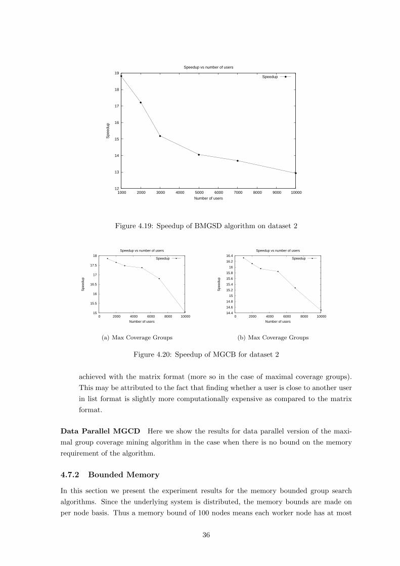
12

13

14

15

16

17

18

19

1000 2000 3000 4000 5000 6000 7000 8000 9000 10000

Spe

edup

Number of users

Speedup vs number of users

Speedup

Figure 4.19: Speedup of BMGSD algorithm on dataset 2

15

15.5

16

16.5

17

17.5

18

0 2000 4000 6000 8000 10000

Spe

edup

Number of users

Speedup vs number of users

Speedup

(a) Max Coverage Groups

14.4

14.6

14.8

15

15.2

15.4

15.6

15.8

16

16.2

16.4

0 2000 4000 6000 8000 10000

Spe

edup

Number of users

Speedup vs number of users

Speedup

(b) Max Coverage Groups

Figure 4.20: Speedup of MGCB for dataset 2

achieved with the matrix format (more so in the case of maximal coverage groups).

This may be attributed to the fact that finding whether a user is close to another user

in list format is slightly more computationally expensive as compared to the matrix

format.

Data Parallel MGCD Here we show the results for data parallel version of the maxi-

mal group coverage mining algorithm in the case when there is no bound on the memory

requirement of the algorithm.

4.7.2 Bounded Memory

In this section we present the experiment results for the memory bounded group search

algorithms. Since the underlying system is distributed, the memory bounds are made on

per node basis. Thus a memory bound of 100 nodes means each worker node has at most

36

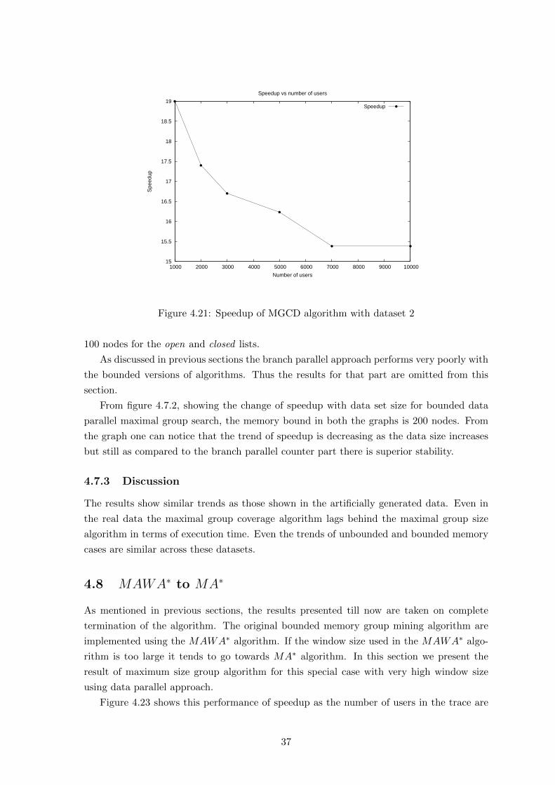
15

15.5

16

16.5

17

17.5

18

18.5

19

1000 2000 3000 4000 5000 6000 7000 8000 9000 10000

Spe

edup

Number of users

Speedup vs number of users

Speedup

Figure 4.21: Speedup of MGCD algorithm with dataset 2

100 nodes for the open and closed lists.

As discussed in previous sections the branch parallel approach performs very poorly with

the bounded versions of algorithms. Thus the results for that part are omitted from this

section.

From figure 4.7.2, showing the change of speedup with data set size for bounded data

parallel maximal group search, the memory bound in both the graphs is 200 nodes. From

the graph one can notice that the trend of speedup is decreasing as the data size increases

but still as compared to the branch parallel counter part there is superior stability.

4.7.3 Discussion

The results show similar trends as those shown in the artificially generated data. Even in

the real data the maximal group coverage algorithm lags behind the maximal group size

algorithm in terms of execution time. Even the trends of unbounded and bounded memory

cases are similar across these datasets.

4.8 MAWA∗ to MA∗

As mentioned in previous sections, the results presented till now are taken on complete

termination of the algorithm. The original bounded memory group mining algorithm are

implemented using the MAWA∗ algorithm. If the window size used in the MAWA∗ algo-

rithm is too large it tends to go towards MA∗ algorithm. In this section we present the

result of maximum size group algorithm for this special case with very high window size

using data parallel approach.

Figure 4.23 shows this performance of speedup as the number of users in the trace are

37

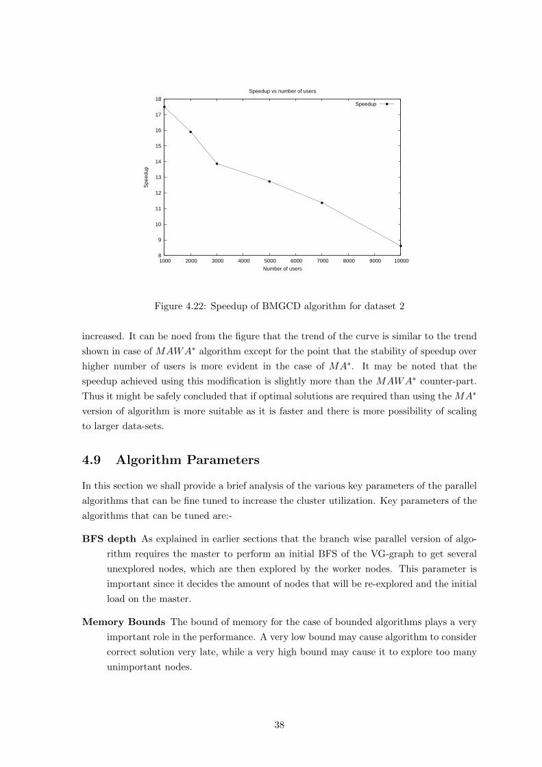
8

9

10

11

12

13

14

15

16

17

18

1000 2000 3000 4000 5000 6000 7000 8000 9000 10000

Spe

edup

Number of users

Speedup vs number of users

Speedup

Figure 4.22: Speedup of BMGCD algorithm for dataset 2

increased. It can be noed from the figure that the trend of the curve is similar to the trend

shown in case of MAWA∗ algorithm except for the point that the stability of speedup over

higher number of users is more evident in the case of MA∗. It may be noted that the

speedup achieved using this modification is slightly more than the MAWA∗ counter-part.

Thus it might be safely concluded that if optimal solutions are required than using the MA∗

version of algorithm is more suitable as it is faster and there is more possibility of scaling

to larger data-sets.

4.9 Algorithm Parameters

In this section we shall provide a brief analysis of the various key parameters of the parallel

algorithms that can be fine tuned to increase the cluster utilization. Key parameters of the

algorithms that can be tuned are:-

BFS depth As explained in earlier sections that the branch wise parallel version of algo-

rithm requires the master to perform an initial BFS of the VG-graph to get several

unexplored nodes, which are then explored by the worker nodes. This parameter is

important since it decides the amount of nodes that will be re-explored and the initial

load on the master.

Memory Bounds The bound of memory for the case of bounded algorithms plays a very

important role in the performance. A very low bound may cause algorithm to consider

correct solution very late, while a very high bound may cause it to explore too many

unimportant nodes.

38

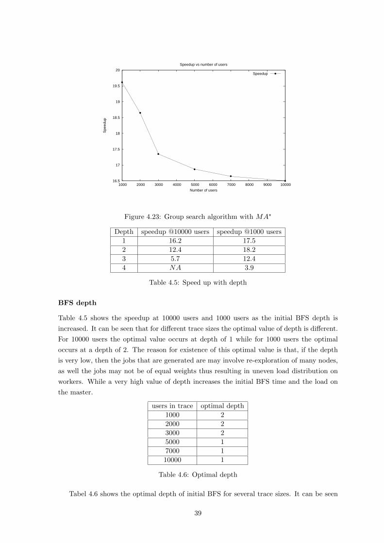
16.5

17

17.5

18

18.5

19

19.5

20

1000 2000 3000 4000 5000 6000 7000 8000 9000 10000

Spe

edup

Number of users

Speedup vs number of users

Speedup

Figure 4.23: Group search algorithm with MA∗

Depth speedup @10000 users speedup @1000 users

1 16.2 17.5

2 12.4 18.2

3 5.7 12.4

4 NA 3.9

Table 4.5: Speed up with depth

BFS depth

Table 4.5 shows the speedup at 10000 users and 1000 users as the initial BFS depth is

increased. It can be seen that for different trace sizes the optimal value of depth is different.

For 10000 users the optimal value occurs at depth of 1 while for 1000 users the optimal

occurs at a depth of 2. The reason for existence of this optimal value is that, if the depth

is very low, then the jobs that are generated are may involve re-exploration of many nodes,

as well the jobs may not be of equal weights thus resulting in uneven load distribution on

workers. While a very high value of depth increases the initial BFS time and the load on

the master.

users in trace optimal depth

1000 2

2000 2

3000 2

5000 1

7000 1

10000 1

Table 4.6: Optimal depth

Tabel 4.6 shows the optimal depth of initial BFS for several trace sizes. It can be seen

39

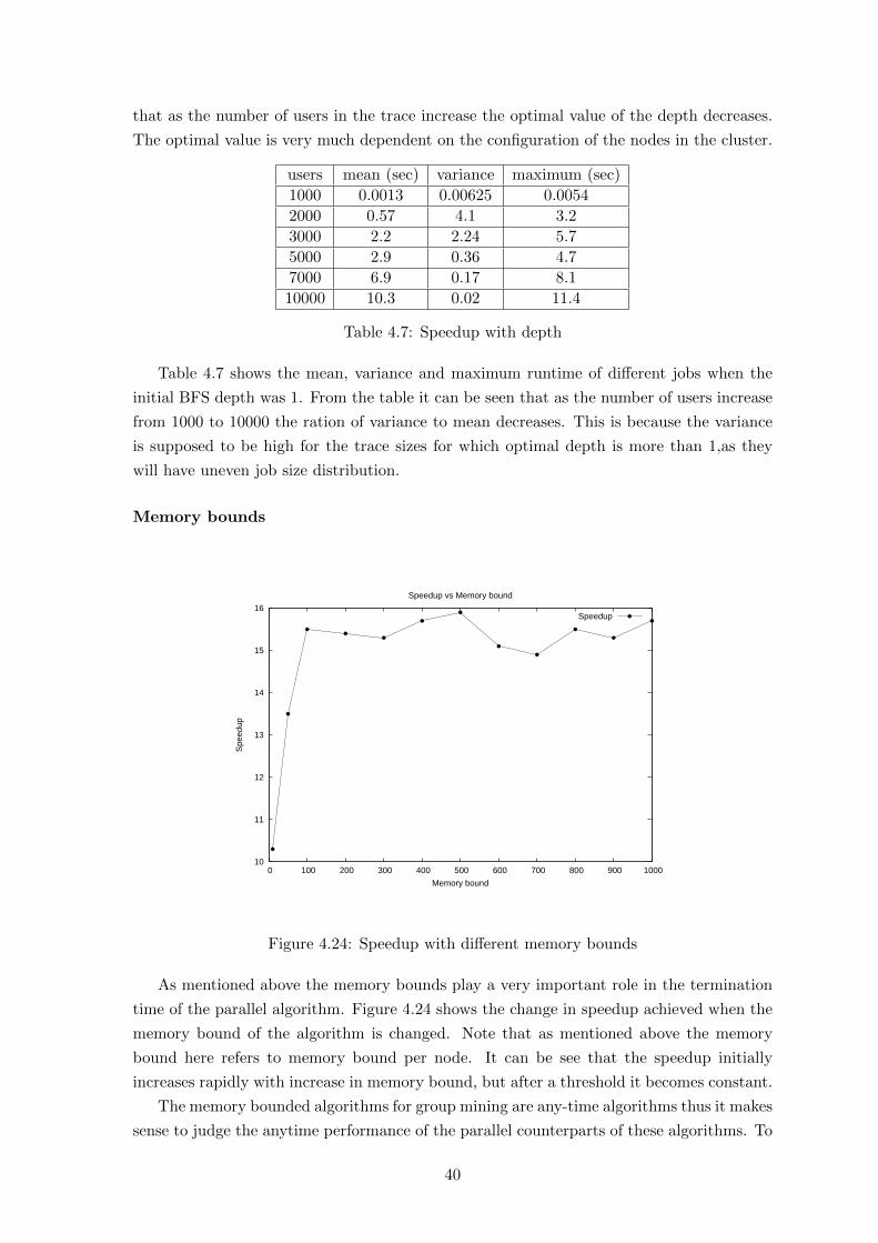
that as the number of users in the trace increase the optimal value of the depth decreases.

The optimal value is very much dependent on the configuration of the nodes in the cluster.

users mean (sec) variance maximum (sec)

1000 0.0013 0.00625 0.0054

2000 0.57 4.1 3.2

3000 2.2 2.24 5.7

5000 2.9 0.36 4.7

7000 6.9 0.17 8.1

10000 10.3 0.02 11.4

Table 4.7: Speedup with depth

Table 4.7 shows the mean, variance and maximum runtime of different jobs when the

initial BFS depth was 1. From the table it can be seen that as the number of users increase

from 1000 to 10000 the ration of variance to mean decreases. This is because the variance

is supposed to be high for the trace sizes for which optimal depth is more than 1,as they

will have uneven job size distribution.

Memory bounds

10

11

12

13

14

15

16

0 100 200 300 400 500 600 700 800 900 1000

Spe

edup

Memory bound

Speedup vs Memory bound

Speedup

Figure 4.24: Speedup with different memory bounds

As mentioned above the memory bounds play a very important role in the termination

time of the parallel algorithm. Figure 4.24 shows the change in speedup achieved when the

memory bound of the algorithm is changed. Note that as mentioned above the memory

bound here refers to memory bound per node. It can be see that the speedup initially

increases rapidly with increase in memory bound, but after a threshold it becomes constant.

The memory bounded algorithms for group mining are any-time algorithms thus it makes

sense to judge the anytime performance of the parallel counterparts of these algorithms. To

40

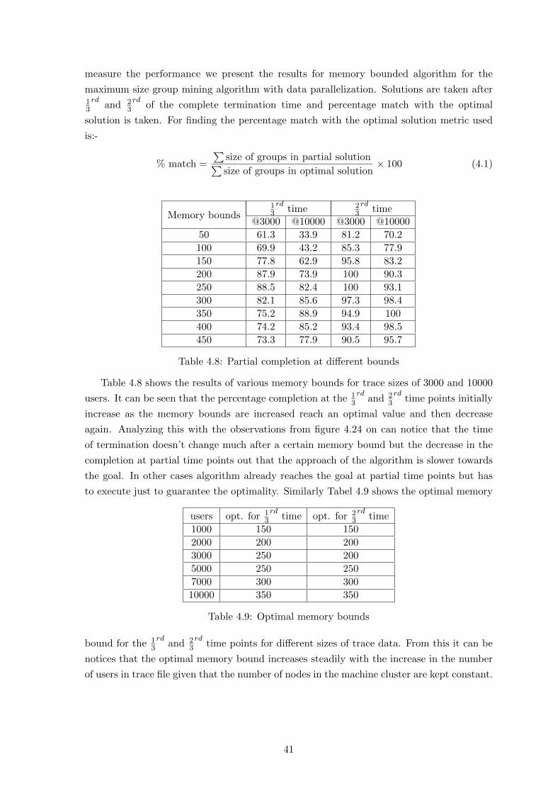
measure the performance we present the results for memory bounded algorithm for the

maximum size group mining algorithm with data parallelization. Solutions are taken after13

rdand 2

3

rdof the complete termination time and percentage match with the optimal

solution is taken. For finding the percentage match with the optimal solution metric used

is:-

% match =

∑size of groups in partial solution∑size of groups in optimal solution

× 100 (4.1)

Memory bounds13

rdtime 2

3

rdtime

@3000 @10000 @3000 @10000

50 61.3 33.9 81.2 70.2

100 69.9 43.2 85.3 77.9

150 77.8 62.9 95.8 83.2

200 87.9 73.9 100 90.3

250 88.5 82.4 100 93.1

300 82.1 85.6 97.3 98.4

350 75.2 88.9 94.9 100

400 74.2 85.2 93.4 98.5

450 73.3 77.9 90.5 95.7

Table 4.8: Partial completion at different bounds

Table 4.8 shows the results of various memory bounds for trace sizes of 3000 and 10000

users. It can be seen that the percentage completion at the 13

rdand 2

3

rdtime points initially

increase as the memory bounds are increased reach an optimal value and then decrease

again. Analyzing this with the observations from figure 4.24 on can notice that the time

of termination doesn’t change much after a certain memory bound but the decrease in the

completion at partial time points out that the approach of the algorithm is slower towards

the goal. In other cases algorithm already reaches the goal at partial time points but has

to execute just to guarantee the optimality. Similarly Tabel 4.9 shows the optimal memory

users opt. for 13

rdtime opt. for 2

3

rdtime

1000 150 150

2000 200 200

3000 250 200

5000 250 250

7000 300 300

10000 350 350

Table 4.9: Optimal memory bounds

bound for the 13

rdand 2

3

rdtime points for different sizes of trace data. From this it can be

notices that the optimal memory bound increases steadily with the increase in the number

of users in trace file given that the number of nodes in the machine cluster are kept constant.

41

4.10 Discussions

In this chapter we produced detailed results of the experiments conducted on the paralleliza-

tion techniques. From the results one can observe that the data parallelization technique

emerges out to be superior to the simple branch parallel technique, which though effective

with unbounded cases, falters when a bound is kept on the memory. Even when comparing

the stability and scalability of the two approaches the data parallel approach emerges better

in terms of both the metrics. It shows much more stable performance across different ver-

sions and shows better trends with increase in data size. Though no conclusive comments

can be made on the scalability as the data set and the cluster size for the experiments is very

less as compared to the expected data size in practical scenarios. In both the figures 4.6.2

and 4.7.2, we can observe that the speedup goes down as the number of users are increased.

Thus the data parallel approach becomes susceptible to network congestion when there is

memory bound on individual workers. There is a slight saturation in the case of maximum

size group search but given the range of data for experiment, nothing conclusive can be

derived.

As per the problem statement the parallelization schemes do achieve the objective of

running the group mining algorithms on machine cluster with appreciable node utilization.

The Branch parallel approach achieves the speedup using the brute power of the individual

machines while the Data parallel approach utilizes the distributed power by finding patterns

in the data and parallelizing it. The experimental results show that best results are obtained

when:-

1. There is no bound on the working memory of the algorithm.

2. There is minimal dependence on the results of other jobs.

3. There is minimal re-exploration of nodes.

4. Load distribution on the workers.

From the experiments conducted in this thesis following verdicts can be passed specific to

the approached discussed in the text:-

1. Parallelizing group mining algorithms that don’t have a bound on the memory is much

easier and better performance-wise as compared to the case of memory bounds. The

DFS algorithm, given its innate parallelism and low dependence on the results of other

branches can be parallelized most effectively.

2. The underlying file system or the distributed system plays a very important role

in the performance of the parallelization schemes. As seen in the previous sections

the variation of the redundancy factor changes the performance of the algorithms.

Similarly it can be conjectured that some better file system can further improve the

performance of the schemes.

3. The verdict on scalability is two fold. Firstly the scalability of the distributed system

concerns about whether the algorithms developed can be used in a bigger cluster. The

42

experimental results show that increase in the speedup is linear with the increase in

the cluster size thus theoretically the algorithms shall be scalable. However given the

small range of cluster sizes for the experimentation nothing can be conclusively said

regarding scalability of the distributed system. The second aspect of the scalability is

that whether the algorithm can retain its performance as the data set size is increased.

From the experimental results it can be seen that while the branch parallel version

shows a steep decline in the performance as data size is increased, the data parallel

version initially decreases but then tends to stabilize. Thus the data parallel version

is more stable with respect to increase in the dataset size.

4. The applicability of the branch parallel scheme on bounded memory cases is very

poor. While the data parallel version performs fine with these versions. Still in the

case of bounded maximum coverage group search where there is high inter dependence

between job the performance of data parallel version decreases rapidly as the dataset

size is increased.

5. The memory bound per node of the cluster also plays a very important factor in the

performance of the parallel algorithm. As observed in the experiments a very low

bound on memory can affect the performance in terms of termination time, higher

bound on memory affect the rate at which algorithm approaches the goal state.

6. With proper memory bounds the performance of anytime algorithms in terms of partial

results is also appreciable. In many cases the algorithm reaches the goal state even

before 23

rdof its actual execution time. This shows that the quality of partial results

produced is very good.

7. Although the preprocessing time is not included in the final results, as depicted in

the results it is comparatively smaller to the actual execution time of the algorithm.

Omission of the preprocessing time may also be reasonable since the preprocessing is

actually just changing the data format. If the data format was initially collected in

the required way, the preprocessing step may not have even been required.

43

Chapter 5

Conclusions

In the present work we proposed two approaches for parallel implementation of specific

group mining algorithms. We analyzed the two approaches on two separate datasets and

concluded that the parallelization techniques are indeed feasible within the scope of study.

The stability and the scalability of the schemes proposed are questionable since the study

was limited to only a small cluster of 20 machines and the data size used never exceeded

10000 users. Next we shall discuss the limitations of the present work and some possible

future work.

5.1 Limitations

The conclusions made herein are limited by the hardware resources available, time and

scope of the problem. The present work only attempts to parallelize the already existing

group mining algorithm, it doesn’t aim to improve the mining algorithm itself or concern

about the quality of the solutions by changing the definition of groups. The experiments were

conducted on a small cluster of size 20 nodes other than the master, thus the scalability of the

distributed system can’t be commented upon. Similarly because of time schedule limitations

the maximum size of dataset used in the experiment is 10000 users, where as the general aim

of parallel group mining algorithms is in the order of 106 users, extrapolations done to make

conclusions about scalability may not work at such large scales. The implementation of the

algorithms was done in python programming language, coding in lower level languages like

Java or C may provide better results. Another important limitation of the current study is

that the algorithms have been tested out only one real dataset. This might not be conclusive

to say that the results will be similar or even comparable if used with some other dataset.

5.2 Future Work

There are some prospects to further expand this work. The experiments can be conducted

on a larger machine cluster to conclusively comment on the scalability of the distributed

system. Similarly simulations on more real world user mobility may give greater insights into

the ways of improving the algorithms. The present schemes can be tested out or modified

according to other definitions of groups and analyzed. Re-implementing the system in lower

44

level languages might also provide better and different results from those discussed here.

More parallelization schemes may be proposed based on the lines of parallel algorithms like

PV-node or PV-cut or dynamic tree splitting (as generally done in multi-core α-β search).

Further more different groups mining algorithms (like based on Born-Kerboch Algorithm)

may be attempted to run on machine clusters and there results compared to the present

work. There can also be an exhaustive study on the variation of the results with change in

algorithm parameters to arrive at conclusive remarks about interrelation of those parameters

and the parallelization of the algorithm.

45

Bibliography

[1] The Hadoop Distributed File System. IEEE, May 2010.

[2] Adam L. Beberg, Daniel L. Ensign, Guha Jayachandran, Siraj Khaliq, and Vijay S.

Pande. Folding@home: Lessons from eight years of volunteer distributed computing. In

Proceedings of the 2009 IEEE International Symposium on Parallel&Distributed Pro-

cessing, IPDPS ’09, pages 1–8, Washington, DC, USA, 2009. IEEE Computer Society.

[3] Jeffrey Dean and Sanjay Ghemawat. Mapreduce: simplified data processing on large

clusters. Commun. ACM, 51(1):107–113, January 2008.

[4] John Goh and David Taniar. Mining frequency pattern from mobile users. In Mircea

Negoita, Robert Howlett, and Lakhmi Jain, editors, Knowledge-Based Intelligent Infor-

mation and Engineering Systems, volume 3215 of Lecture Notes in Computer Science,

pages 795–801. Springer Berlin / Heidelberg, 2004.

[5] Tristan Henderson. CRAWDAD tool tools/process/syslog/syslog-parser (v. 2006-11-

01). Downloaded from http://crawdad.cs.dartmouth.edu/tools/process/syslog/syslog parser,

November 2006.

[6] Tristan Henderson, David Kotz, Ilya Abyzov, and Jihwang Yeo. CRAW-

DAD trace dartmouth/campus/syslog/01-04 (v. 2004-12-18). Downloaded from

http://crawdad.cs.dartmouth.edu/dartmouth/campus/syslog/01 04, December 2004.

[7] San-Yih Hwang, Ying-Han Liu, Jeng-Kuen Chiu, and Ee-Peng Lim. Mining mobile

group patterns: A trajectory-based approach. In PAKDD, pages 713–718, 2005.

[8] John Nickolls, Ian Buck, Michael Garland, and Kevin Skadron. Scalable parallel pro-

gramming with cuda. Queue, 6(2):40–53, March 2008.

[9] S. Tucker Taft. Multicore programming in parasail: parallel specification and imple-

mentation language. In Proceedings of the 16th Ada-Europe international conference

on Reliable software technologies, Ada-Europe’11, pages 196–200, Berlin, Heidelberg,

2011. Springer-Verlag.

[10] S.G. Vadlamudi, S. Aine, and P.P. Chakrabarti. A memory-bounded anytime heuristic-

search algorithm. Systems, Man, and Cybernetics, Part B: Cybernetics, IEEE Trans-

actions on, 41(3):725 –735, june 2011.

46