Computer Physics Communications 190 (2015) 173–181

Contents lists available at ScienceDirect

Computer Physics Communications

journal homepage: www.elsevier.com/locate/cpc

Parallel AFMPB solver with automatic surface meshing for calculationof molecular solvation free energyI

Bo Zhanga, Bo Pengb, Jingfang Huang c, Nikos P. Pitsianis d,e, Xiaobai Sune, Benzhuo Lub,⇤a Center for Research in Extreme Scale Technologies, Indiana University, IN, USAb State Key Laboratory of Scientific/Engineering Computing, Institute of Computational Mathematics and Scientific/Engineering Computing, Academy ofMathematics and Systems Science, Chinese Academy of Sciences, Beijing 100190, Chinac Department of Mathematics, the University of North Carolina at Chapel Hill, NC, USAd Department of Electrical and Computer Engineering, Aristotle University, Greecee Department of Computer Science, Duke University, NC, USA

a r t i c l e i n f o

Article history:Received 11 August 2014Received in revised form23 November 2014Accepted 25 December 2014Available online 23 January 2015

Keywords:Poisson–Boltzmann equationBoundary integral equationAutomatic surface meshingSolvation free energyFast multipole methodsParallelizationCilk Plus

a b s t r a c t

We present PAFMPB, an updated and parallel version of the AFMPB software package for fast calculationof molecular solvation-free energy. The new version has the following new features: (1) The adaptivefast multipole method and the boundary element methods are parallelized; (2) A tool is embeddedfor automatic molecular VDW/SAS surface mesh generation, leaving the requirement for a mesh file atinput optional; (3) The package provides fast calculation of the total solvation-free energy, includingthe PB electrostatic and nonpolar interaction contributions. PAFMPB is implemented in C and Fortranprogramming languages, with the Cilk Plus extension to harness the computing power of both multicoreand vector processing. Computational experiments demonstrate the successful application of PAFMPB tothe calculation of the PB potential on a dengue virus systemwithmore than onemillion atoms and ameshwith approximately 20 million triangles.

Program summary

Program title: Parallel AFMPBCatalogue identifier: AEGB_v2_0Program summary URL: http://cpc.cs.qub.ac.uk/summaries/AEGB_v2_0.htmlProgram obtainable from: CPC Program Library, Queen’s University, Belfast, N. IrelandLicensing provisions: GNU General Public License, version 2No. of lines in distributed program, including test data, etc.: 40558No. of bytes in distributed program, including test data, etc.: 2349976Distribution format: tar.gzProgramming language: Mixed C and Fortran, Compiler: Intel or GNU with Cilk Plus enabled.Computer: Any, but the code is mainly designed for multicore architectures.Operating system: Linux.RAM: Depends on the size of the discretized biomolecular system.Classification: 3.Catalogue identifier of previous version: AEGB_v1_1Journal reference of previous version: Comput. Phys. Comm. 184 (2013) 2618External routines: Users are allowed to use external routines/libraries (e.g., MSMS [6] and TMSMesh [4])to generate compatible surface mesh input data if they choose not to use the embedded automatic meshgeneration tool in the package. Post-processing tools such as VCMM [5] and VMD [3] can also be used forvisualization and analyzing results.

I This paper and its associated computer program are available via the Computer Physics Communication homepage on ScienceDirect (http://www.sciencedirect.com/science/journal/00104655).⇤ Corresponding author.

E-mail address: bzlu@lsec.cc.ac.cn (B. Lu).

http://dx.doi.org/10.1016/j.cpc.2014.12.0220010-4655/© 2015 Elsevier B.V. All rights reserved.

174 B. Zhang et al. / Computer Physics Communications 190 (2015) 173–181

The package uses two subprograms: (1) The iterative Krylov subspace solver, SPARSKIT, from Yousef Saad[2]; and (2) Cilk-based parallel fast multipole methods from FMMSuite [1].Does the new version supersede the previous version? YesNature of problem: Numerical solution of the linearized Poisson–Boltzmann equation that describeselectrostatic interactions of molecular systems in ionic solutions.Solution method: The linearized Poisson–Boltzmann equation is reformulated as a boundary integralequation and is subsequently discretized using the node-patch scheme. The resulting linear system issolved using Krylov subspace solvers iteratively. The reformulation of the equation provides an upperbound for the number of iterations. Within each iteration, thematrix–vector multiplication is acceleratedusing the adaptive plane-wave expansion based fast multipole methods. The majority of the codes areparallelized using the Cilk runtime.Reasons for new version: New functions are added and a few old functions like force calculations areremoved. The algorithm is parallelized and most parts of the code are rewritten.Summary of revisions: The computation is parallelized and an automatic mesh generationmethod for BEMis added.Restrictions: The program has only been tested on machines running Linux operating system.Additional comments: The Cilk runtime used in the development and testing is from the Intel compilerSuite. The GNU Cilk Plus and Cilk Plus/LLVM branches have not been tested.Running time: The running time depends on the number of discretized elements (N) and their distribution.It also depends on the number of cores used in the computation.References:[1] http://www.fastmultipole.org/.[2] http://www-users.cs.umn.edu/~saad/software/.[3] http://www.ks.uiuc.edu/Research/vmd/.[4] http://www.continuummodel.org.[5] S. Bai, B. Lu, VCMM: A visual tool for continuum molecular modeling. J. Mol. Graph. Model. 50 (2014)44–49.[6] Scanner, F. Michel, Olson, J. Arthur, Spehner, J. Claude, Reduced surface: An efficient way to computemolecular surfaces. Biopolymers 38 (1996) 305–320.

© 2015 Elsevier B.V. All rights reserved.

1. Introduction

The Poisson–Boltzmann (PB) equation has been widely used tomodel the electrostatic properties of biomolecules, membranes,colloids, polyelectrolytes, and macromolecular objects. Efficientnumerical solution of PB equations has been an active researchtopic in scientific computing. Many algorithms have been in-troduced, including the multigrid method [1], precorrected-FFTmethod [2], tree code [3], and the fast multipole method (FMM)[4–7]. These algorithms reduce the computational complexity fromO(N2) to O(N logN), or asymptotically optimal O(N), where Nis the problem size. However, the efficiency was not satisfactorywhen the PB calculation was applied to the macromolecular sys-tems or an ensemble of molecular structures.

Substantial progress has beenmade in improving the efficiencyof PB calculations, such as the use of many-core graphic process-ing units (GPUs) accelerators [8,9], distributed and shared mem-ory programming via MPI and OpenMP [1,10–12]. In the work byGeng et al. [10], a parallel higher-order boundary integral equationmethod is implemented using MPI.

In this paper, we present a parallel version of the adaptive fastmultipole Poisson–Boltzmann equation solver (PAFMPB). Signifi-cant differences from the previous sequential AFMPB package [6]are: (1) PAFMPB targets multicore computer architectures andutilizes Cilk Plus [13] for parallelization. (2) PAFMPB adds an in-tegrated automatic mesh generation option to handle the circum-stance when an external mesh file is not easily obtainable or themesh quality is not satisfactory for numerical simulation. (3) The

computation of the total solvation-free energy contains both polarand nonpolar energy terms. (4) PAFMPB is written in mixed C andFortran programming languages. In preliminary numerical experi-ments with PAFMPB, we have observed substantial improvementsin terms of parallel efficiency and memory usage.

The rest of the paper is organized as follows. In Section 2, webriefly describe the individual elements of the PAFMPB package,namely, the PB model, the boundary integral equation (BIE) re-formulation, the surface mesh generation method, the node-patchdiscretization approach, the Krylov subspace method, fast multi-pole method with plane-wave expansion, and the Cilk Plus sys-tem for parallelization. We present the code structure in Section 3.Preliminary numerical results are presented in Section 4 to demon-strate the accuracy and parallel performance of the solver.We con-clude the paper in Section 5.

2. Mathematical models and discretization methods

We first give a brief review of the mathematical theories andcomputational methods that underlie the PAFMPB package. Wethen detail the new features in PAFMPB, in addition to that in [6]and references therein.

2.1. Continuum electrostatic models and boundary integral equations

Electrostatic interactions within and between molecules inelectrolyte solution have long been recognized as playing a varietyof important roles in determining molecular structure and binding

B. Zhang et al. / Computer Physics Communications 190 (2015) 173–181 175

activity. Consider a molecule immersed in an electrolyte solution.The interior region (molecule) and the exterior region (solvent) aredenoted by ⌦1 and ⌦2, respectively. The interior potential �int(r)is governed by the Poisson equation

� r · (✏intr�int(r)) =MX

i=1

qi�(r, ci) for r 2 ⌦1. (1)

The exterior potential �ext(r) is governed by the Poisson–Boltzmann equation [14]. In this work, we use an approximatedform of the PB equation, specifically, the linearized PB (LPB) equa-tion as follows:

� r · (✏extr�ext(r)) = �2�ext(r) for r 2 ⌦2. (2)

Here, ✏int denotes the dielectric constant inside the molecule, andthe molecule (the right-hand side of Eq. (1)) is represented by Mpoint charges qiec at positions ci, i = 1, 2, . . . ,M . The reciprocalof the Debye length 1/ characterizes the screening effect due tothe surrounding electrolyte solution. At molecular surface � , thepotential and the normal component of the electric displacementmust be continuous,

�int = �ext and ✏int@�int

@n= ✏ext

@�ext

@n, (3)

where n denotes the outward unit normal vector to the molecularsurface and ✏ext is the dielectric constant of the electrolyte solution.

Both equations in (1) and (2) can be recast into boundary in-tegral equations (BIEs) using Green’s second identity. In fact, awell-conditioned second kind Fredholm integral equation can beobtained through a combination of the BIEs and derivative formsof the BIEs [6]:✓

12✏

+ 12

◆fp =

I

S

(Gpt � upt)ht

�✓1✏

@Gpt

@n� @upt

@n

◆ft�dS + 1

✏ext

X

k

qkGpk

✓12✏

+ 12

◆hp =

I

S

✓@Gpt

@n0� 1

✏

@upt

@n0

◆ht

� 1✏

✓@2Gpt

@n0@n� @2upt

@n0@n

◆ft�dS + 1

✏ext

X

k

qk@Gpk

@n0. (4)

Here, ✏ = ✏ext✏int

, n0 and n are the unit normal vectors at point p 2� and t 2 � , respectively.We denote by fp and hp the values of�ext

and @�ext

@n at point p, respectively. Wemake use of the fundamentalsolutions to the Poisson equation Gpt and the LPB equation upt ,

Gpt = 14⇡ |rt � rp|

, upt = exp(�|rt � rp|)4⇡ |rt � rp|

.

2.2. Molecular surfaces and mesh generation

Numerical solution of the BIEs in Eq. (4) requires a discretizationof the molecular surfaces, namely, a mesh. The previous version ofAFMPB requires a mesh file as an input file. The mesh may be gen-erated using existing packages such as MSMS [15] (for solvent ex-cluded surface (SES) mesh generation). The mesh generation maybe considered as a preprocessing step, separated from the AFMPBexecution. Besides the inconvenience, some inconsistencymay oc-cur between the mesh generation and the AFMPB requirement. InPAFMPB, in addition to accepting external mesh files as input, weprovide an embedded meshing procedure that can discretize boththemolecular van derWaals (VDW) surface and solvent-accessiblesurface (SAS) into triangular or quadrilateral patches, which are to

be used directly in the node-patch discretization discussed in thenext section. For large molecules, we make use of the recently de-veloped TMSmesh package for generating triangular surface meshfor the molecular Gaussian surface [16], which is smooth and an-alytically differentiable with respect to the position of atoms. Inthe rest of this section, we describe the automatic mesh genera-tion procedure for VDW/SAS surface mesh and TMSmesh [17,16]for Gaussian surface mesh generation, respectively.

Different definitions of themolecular surface (the boundary be-tween the solute and the solvent) can affect the PB calculation re-sults. Zhou et al. [18] compared theVDWsurface andmolecular SESwhen applied in the PB calculations and concluded that the VDWsurface may yield better results than the molecular SES.

2.2.1. An auto-meshing procedureIn PAFMPB, an auto-meshing option is provided to conveniently

generate meshes for either the SAS or VDW molecular surfaces.The latitude–longitude based method discretizes the surface intoeither triangular or quadrilateral patches. These patches can bedirectly used in the node-patch BEM [19], which needs only thenormal, area, and centroid coordinates for each node patch. Themethod shares similar features as the program developed by Leeand Richard [20], including the estimate of the SAS area and staticaccessibility.

Following the convention in the study of biomolecular sys-tems, we represent a molecule as a set of overlapping spheres,and define the VDW or SAS surface as the topological boundaryof the spheres as follows: the set of atomic spheres is denoted as{O1,O2, . . . ,OM}, each with radius ⇢i = RVDW

i + Rp, where RVDWi is

the VDW radius, and Rp is a user-controllable parameter for differ-ent types of surfaces. When Rp = 0, the surface is the VDW surfaceand when Rp = Rwater = 1.4 Å, the surface is the SAS surface.

Our mesh generation subroutine consists of two stages. In thefirst stage, each spherical surface is discretized using suitable lat-itude and longitude lines to form surface elements and their ar-eas and normal directions are calculated. For each sphere Oi, thespherical surface is discretized by dividing the azimuthal angle �(from 0 to 2⇡ ) into n equispaced intervals, 0 = �0 < �1 < · · · <�n�1 < 2⇡ , and dividing the sine of the polar angle ✓ (from �1to 1) into m equispaced intervals, �⇡

2 = ✓0 < ✓1 < · · · <✓m = ⇡

2 . We define [�j, �j+1] ⇥ [✓k, ✓k+1] as one element. Its areais ⇢2

i (sin ✓k+1 � sin ✓k)(�j+1 � �j), and its normal direction is✓cos

✓k + ✓k+1

2cos

�j + �j+1

2, cos

✓k + ✓k+1

2

sin�j + �j+1

2, sin

✓k + ✓k+1

2

◆.

The surface discretization in this step generates l elements ei,1,. . . , ei,l for sphere i, l = mn.

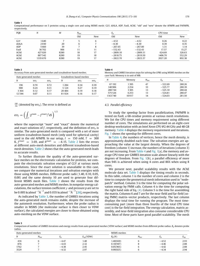
In the second stage, we modify any element whose centralpoint is located inside any sphere(s). Such elements are referredto as ‘‘buried elements’’. For each Oi, we find all its intersectingsphere(s), and then check whether each element ei,j is a buried el-ement, 1 6 j 6 l. Non-buried elements are added to the surfacepatch list directly. A two-atom system using the above method isillustrated in Fig. 2.

This algorithm is simple, but has quadratic complexity inM , thenumber of patches. We thereby recommend this automatic mesh-ing option only formodest sizemolecules. Formacromolecules, ex-ternal mesh generation tools should be applied, as in the originalAFMPB package. Particularly, we recommend the recently devel-oped TMSmesh package for generating macromolecular surfacemeshes for the BIE formulation.

Efficient generation of a high-qualitymesh has been a challeng-ing problem to the scientific computing community for decades.

176 B. Zhang et al. / Computer Physics Communications 190 (2015) 173–181

Mesh generation remains a major bottleneck for computationallyintensive electrostatic analysis. To further improve efficiency, weare currently investigating (1) octree-structure based schemes toreduce the complexity of the latitude–longitude based method;(2) proper parameterization procedure and higher order geomet-ric representation to reduce the number of elements; and (3) fastmesh modification strategies when the shape of the moleculechanges slightly at each time step. New resultswill be incorporatedin future releases of the PAFMPB package.

2.2.2. TMSmesh and Gaussian molecular surfaceFor a macromolecular system, it has been a long-standing chal-

lenge to generate a high-quality mesh. We recently developeda robust program, TMSmesh [16], for generating macromolecularGaussian surfaces and the corresponding meshes.

The Gaussian molecular surface is defined as a level set of thesummation of the Gaussian kernel functions as follows:

�(x) =MX

i=1

e�d(|x�ci|2�⇢2i ) = 1, x 2 R3, (5)

where ci and ⇢i are the location and radius of atom i, respectively,and d is a positive parameter controlling the decay speed ofthe kernel functions. Compared to the VDW and SAS surfaces,the Gaussian surface is usually smooth, without corner or edgesingularities. In addition, it is possible to adjust the parameter dto approximate other types of surfaces.

In TMSmesh, a trace technique is used to mesh the Gaussiansurface. The program has a linear computational complexity in thenumber of atoms, and is capable of treating arbitrarily largemacro-molecules. An example of Gaussian surface mesh for the denguevirus system consisting of 1082160 atoms is shown in Fig. 3(a),with 9758 426 vertices and 19 502 784 elements. TMSmesh hasalso been used to stably generate meshes for other systems suchas the 70S ribosome [16]. The mesh quality has been validated bycomparisonswithmeshes fromother programs, and by the simula-tion results for the BIE-based newversion of the AFMPB solver. Fur-ther details of the algorithms and comparisons can be found in [16].

2.3. Discretization and the ‘‘node-patch’’ method

We adopt a ‘‘node-patch’’ approach to discretize the BIEs inEq. (4). The approach can be considered as a modified linear el-ement method in accuracy but it takes advantage of the ease ofprogramming as for the constant element method. Using the gen-erated closed mesh approximation of the molecular boundary � ,the unknowns in the traditional linear elementmethod are definedat the vertices, and the surface function f (r), r 2 � , is approxi-mated by f (r) = PV

k=1 fkNk(r) using the linear element basis func-tions {Nk(r), k = 1, 2, . . . , V }, where V is the number of verticesin the mesh of � , fk is the value of f (r) at vertex k, and Nk(r) is apiecewise linear functionwhich equals 1 at node k and 0 at all othernodes. Similarly, we have h(r) = PV

k=1 hkNk(r). The discretizedform of Eq. (4) becomes✓

12✏

+ 12

◆fp = 1

✏ext

X

k

qkGpk

+VX

k=1

X

t2'(k)

hk

Z

St

�Gpt � upt

�NkdSt

� fkZ

St

✓1✏

@Gpt

@n� @upt

@n

◆NkdSt

�

✓12

+ 12✏

◆hp = 1

✏ext

X

k

qk@Gpk

@n0

+VX

k=1

X

t2'(k)

hk

Z

St

✓@Gpt

@n0� 1

✏

@upt

@n0

◆NkdSt

�VX

k=1

X

t2'(k)

fkZ

St

1✏

✓@2Gpt

@n0@n� @2upt

@n0@n

◆NkdSt (6)

where '(k) is the set of indices for surface elements that containvertex k on themesh for� . Notice that in Eq. (6), one needs to com-pute the nearly-singular and singular integrals representing theconvolution of Green’s function (and its derivatives) with a linearfunction. For efficiency, in the ‘‘node-patch’’ BEM approach [19], apatch is formed around each vertex (node), and the function is as-sumed to be a constant on the node-patch, namely, the functionon each element is a piecewise constant (non-continuous) func-tion.When the node-patch is carefully designed, one should expectcomparable accuracy to that with the linear elementmethods. Oneneeds to compute only the convolution of theGreen’s functionwitha piecewise constant function. The node-patch discretization leadsto a linear system Ax = b, where x denotes the unknowns, A andb are the coefficient matrix and right hand side of Eq. (6), respec-tively.

The node-patch approach has several advantages. (1) The totalnumber of unknowns is reduced for a prescribed accuracy require-ment when compared with the constant element method, hencereducing the computational cost when solving the resulting linearsystem. (2) When the matrix is split into the near and far fieldsA = Anear + Afar, the calculation and storage process of Anear bythe node-patch approach are more economic compared with thelinear element approach. (3) The source and target points are theone and same set of nodes, like the constant element method, al-lowing the application of the symmetric FMM from the FMMSuitepackage [19].

2.4. The Krylov subspace method for solving a linear system

For the discretized linear system, the PAFMPB solver searchesfor the optimal least-squares approximation of the solution in theKrylov subspace Km(A, r0) = span{r0, Ar0, . . . , Am�1r0} for m > 1,where r0 is the initial residual. As the resulting linear system is ingeneral nonsymmetric, the GMRES, biconjugate gradient stabilized(BiCGStab), and transpose-free Quasi-Minimum Residual (TFQMR)can be applied. In the current version of PAFMPB, the subroutinesfrom the open source package SPARSKIT [21] are used, whichfollow the ‘‘reverse communication protocol’’ with a simple andeffective interface for integrating the iterative subroutines with auser-customized matrix–vector product procedure.

The convergence of a Krylov subspace method depends on theinitial guess and eigenvalue distribution of the linear system. Inthe current implementation, the right hand side is used as theinitial guess, as the formulation is already a Fredholm secondkind equation.We are investigating possible approaches to furtherimproving the efficiency of the Krylov iterative approach, by nu-merically preconditioning the linear system resulting from theFredholm second-kind integral equation formulation, and by fur-ther exploiting the parallel potential of the Krylov subspacemethod.

2.5. The fast multipole method with plane wave expansion

Each step of the Krylov subspace method involves a ma-trix–vector multiplication, for which the FMM takes O(N) opera-tions while the direct evaluation takes O(N2) operations, where Nis the dimension of linear system. In the PAFMPBpackage,we applythe new version of the fast multipole method [22], which lowersthe time and space complexity further by a significant factor.

B. Zhang et al. / Computer Physics Communications 190 (2015) 173–181 177

The use of plane wave expansions is the main difference be-tween the original version of the FMM and its new version. TheFMM arrives at the linear-scaling, asymptotically optimal com-plexity by exploiting themathematical properties with novel com-putation mechanisms. The basic observation is that the submatrixcorresponding to the interactions between sources and targets thatare sufficiently far apart is of low rank, bounded from above by aconstant. The basic idea is to partition the interacting particles intofar and near-neighbors, and partition them recursively at multiplespatial scale levels. The FMMhas a simple spatial partition scheme,which is described in a data structure such as an octree for the 3Dcase. The root node represents a box enclosing all the source andtarget particles. The root box is partitioned in halves in each di-mension into eight children boxes. Each child box is partitionedthe same way, recursively. The far–neighbor particle interac-tions are then orchestrated into the interactions between particleensembles in far–neighbor boxes at multiple levels. Each sub-matrix corresponding to the particle interactions between a pair offar–neighbor boxes is of lower rank. The information in each sourcebox is aggregated up to the parent box, passed across at the samelevel to designated far–neighbor boxes, according to the interac-tion lists. The accumulated potential at each target box is disaggre-gated down to its children boxes. In its original version, the FMMrepresents and compresses the entire interaction matrix in termsof translationmatrices via the classical spherical harmonics expan-sions [23]. In its new version [22], the FMM uses the plane waveor exponential expansions to diagonalize the up, down and acrosstranslations, and hence further reduces the translation and inter-action complexity.

2.6. Cilk Plus and PAFMPB

A major change in PAFMPB package lies in parallelizing theFMM and BEM components to utilize multicore computer archi-tectures. Here, parallelizing the algorithms can be considered astraversing the directed acyclic graph (DAG) of the computation de-pendencies in parallel. We point out that the problem of paralleltraversing a DAG of N nodes in the shortest time, with the numberof processing units constant (more than two) is NP-complete [24].We study strategies for near-optimal solutions.

An earlier strategy studied was reported in [25], based on adynamic prioritization scheme, implemented using Pthreads. Theidea is to rank the nodes in the DAG adaptively when the numberof nodes is far more than the number of available processing units.Particularly, the ranking is based on the longest path of each nodeto the final sink node. When two frontier nodes are of the samerank, an ordered pair is associated with each node c , defined ashd�

m(c), ns(c)i,d�m(c) = min

(c,d)2E(G)deg�(d), (7)

where (c, d) is a directed edge from c to d in the edge set E(G), anddeg�(d) is the in-degree at node d. When d�

m(c) = 1, ns(c) equalsthe number of direct successors of c with in-degree 1. That is, cis the only node in the way to release and enable these successornodes. Otherwise, ns(c) equals the out-degree of c , deg+(c). Thecompletion of c makes its successors one step closer to the front.For two equal-ranked nodes u and v, we give u a higher priority if

hd�m(u), �ns(u)i < hd�

m(v), �ns(v)i (8)

in the lexicographical order. If the two nodes have the same pri-ority, a random selection is applied to break the tie. Essentially,the dynamic prioritization approach implemented in [25] can beviewed as a work-sharing approach, where available tasks are putin a priority queue based on their rank for available processingunits. Notice that mutual exclusion is needed for operations on

the queue and this could become a bottleneck when the numberof processing units increases.

More recently, we adopted an alternative approach to paral-lelizing the traversal of FMM DAG and the BEM components usingCilk Plus. Cilk Plus is an extension to the C/C++ language. It intro-duces three new keywords to express data and task parallelism.New tasks can be spawned using cilk_spawn and cilk_forand synchronized usingcilk_sync. The runtime scheduler of CilkPlus creates a worker thread for each processor core present on asystem. Each worker maintains a double-ended queue (deque) forstoring tasks yet to be executed. When a worker thread executes acilk_spawn or cilk_for statement, it simply pushes new tasksonto the tail of its deque. Unlike thework-sharing approach in [25],the scheduler of the Cilk Plus runtime implements a work-stealingschemewith a proven performance guarantee [13].When aworkerhas no work to do, it steals a task from the front of some otherworker’s deque. The Cilk Plus compiler and runtime is supportedin the Intel compiler toolchain as well as in the open source com-pilers from the GCC and the LLVM. Our experiments show that CilkPlus-based parallel FMM solvers are easy to manage and performbetter than the dynamic prioritization code using Pthreads.

2.7. Evaluating the total solvation-free energy

In PAFMPB, an empirical approach is provided to compute thenonpolar contribution to the solvation free energy, which dependson the molecular surface area and volume. The related parame-ters are user-specified in the input file. Combining the polar (elec-trostatic) and nonpolar contributions, the total free energy can becomputed as

�E = �Ep + �Enp. (9)

The nonpolar term, �Enp, includes the energetic cost of cavity for-mation, solvent rearrangement and solute–solvent dispersion in-teractions introduced when the uncharged solute is brought fromvacuum into the solvent environment. The polar term �Ep is de-termined by the PB solution.

The solute charge generates a Coulombic potential field and po-larizes the solvent, which in turn generates a reaction potential inthe solute. The electrostatic potential of a molecule can thereforebe expressed as the sum of the Coulomb potential �c and reactionfield potential �r induced by solvent polarization:

�(r) = �c + �r.

Once the electrostatic potential �(r) is obtained, the electrostaticcontribution of solvation-free energy is computed by

�Ep = 12

MX

i=1

qi�r(ri)

= 12

MX

i=1

qiI

S

✓Git

@�intt

@n� @Git

@n�intt

◆dSt

= 12

MX

i=1

qiX

t

✓✏Githt�St � @Git

@nft�St

◆.

The nonpolar solvation energy depends on the surface area andvolume:

�Enp = � S + pV + b (10)

where S andV are the surface area and volume of the cavity createdby the molecule, respectively, and � , p and b are fitted param-eters, predefined in the input file. Parameter � has the dimen-sions of a surface tension coefficient, parameter p has the pressuredimensions, and parameter b has the energy dimensions. They

178 B. Zhang et al. / Computer Physics Communications 190 (2015) 173–181

depend on the force field and the definition of molecular sur-face because the atomic radii and charges (from the force field)and the surface definition determine together the boundary be-tween the solvent and the solute and, therefore, the surface areaS, volume V and the polar contributions to free energies. For in-stance, the particular values � = 0.005 kcalmol�1�2, p =0.035 kcalmol�1�3 and b = 0 kcalmol�1 are used in [26].In this paper, we omit the attractive nonpolar solvation interac-tions, for the same reason given in [26]. We mention that thenonpolar solvation energy expressions similar to Eq. (10) can bederived using the scaled particle theory [27]. A more detailedinformation for the evaluation of these terms is given in [28].Eq. (10) reduces to the popular area-only nonpolar implicit solventmodel when p = 0 [29,30]. In addition, b is set to 0 kcalmol�1 inall the following test examples of this work.

3. Code structure and implementation

PAFMPB features parallelized FMMs and dynamicmemory allo-cation,making it possible to study protein systemswithmillions ofatoms. In addition, an auto-discretizationmethod for the VDW/SASsurfaces and an empirical formulation for calculating the nonpo-lar solvation energy are implemented to facilitate the use of thepackage. Another feature is the introduction of Linux command-line tools that can load and analyze the input file and accuratelytrack the memory consumption.

In the following, we describe portability and installation of thepackage, several utility tools, file formats and I/O layers, and jobrunning samples.

3.1. Portability and installation

PAFMPB is programmed mostly in ANSI C and Fortran 77.Memory allocation functions from the standard C library are used.After the user downloads the package, the following directories canbe found upon extraction:

• src: contains the driver program afmpb-main.c, the inter-face file afmpb-compute.c, and utility file afmpb-utils.c.File afmpb-solve.c provides routines for BEM calculation.Files fmm-graph.c, fmm-laplace.c, fmm-yukawa.c andfmm-utils.c provide the parallelized FMM for Laplace andYukawa kernels. File afmpb-automesh.c provides the automesh generation. File sparskit.f provides the Krylov sub-space iterative solver [21].

• include: contains header files adap_fmm.h and afmpb.hthat define data types and declare function prototypes.

• example: contains one README file, two sample job files(job.sh and job-automesh.sh), and the generated files(input.txt and output.txt).

• tools: containsmeshgeneration tools, including the TMSmeshtool. Details about these tools are provided in the next section.

In addition, a Makefile is supplied. The current package isbased on Intel compiler and Linux command-line environments.The environment variable LD_LIBRARY_PATH for the librarylibcilkrts.so should be added before compiling and runningPAFMPB.

3.2. Utility tools

The directory tools contains tools for mesh generation. Onescript (pqrmsms.sh) and two executable files (MSMS, TMSmesh)are provided. Given a PQR file (e. g. fas2.pqr in the directory), aMSMS format mesh can be generated by running the command

./pqrmsms.sh fas2.pqr 4 1.4

The last two parameters specify the node density (in the unit of 1per Å2) and probe radius in the unit of Å, respectively. One can alsouse TMSmesh (available at www.continuummodel.org) to gener-ate an OFF format mesh by running the command

./TMSmesh fas2.pqr 0.6 2.0

Themolecule and calculated surface potential can be visualizedand analyzed using our visualization program VCMM [31], or thetool VMD as described in our previous version of AFMPB [6].

3.3. Job execution

PAFMPB is executed in a terminal environment, accepting thefollowing parameters from the command line:

• -i: followed by input file name.• -o: followed by output file name.• -s: followed by surface potential file name.• -t: followed by an integer number (the number of cores used).

PAFMPB expects the following input files: (a) a control parameterfile (input.txt by default), (b) a PQR file containing atomiccharges and their locations, and (c) a molecular surface mesh filewhen the auto meshing function is not used.

A log file (output.txt by default) and a surface potential file(default: surfp.dat) are generated automatically at the comple-tion of PAFMPB execution.

The sample input files and job script files can be found in theprogram package and on our website www.continuummodel.org.A web server will also be provided.

4. Numerical results

In this section, we present numerical results for several testcases. In all cases, the relative dielectric constants are set to be2 inside the molecule and 80 in the electrolyte solution, themonovalent ionic concentration is 150 mM, and the temperatureis 300 K. Unless stated otherwise, N ,M and Niter denote the degreeof freedom of the system (2 times the number of vertices), numberof atoms in protein, and numbers of GMRES iterations for solvingthe LPB, respectively. The unit of the polar and nonpolar solvationenergies is kcal/mol and the CPU time is measured in seconds.

4.1. Accuracy and efficiency of PAFMPB

We solve the LPB and compute the electrostatic solvationenergy on a series of proteins with PAFMPB and previous versionsof AFMPB. The numerical results are reported in Table 1. Thefirst column is the molecule name. Columns 4 and 5 give thenumbers of GMRES iterations for solving the LPB. We notice thatboth AFMPB solvers convergewithin 20 iterations, due to thewell-conditioned integral equation formulation. Columns 6 and 7 reportthe polar solvation energies; results from different versions arevery similar. The last two columns show the CPU time. Because ofcode optimization, the updated version shows better performance,especially for large systems.

4.2. Assessment of auto-generated mesh quality

For small molecules, PAFMPB works well using the automati-cally generated surface mesh. In this section, we first consider aspherical cavity. Since the analytical solution is available, to assessthe accuracy of the auto-generated mesh, we measure the errorsin the potential � (denoted by errf ) and in the normal derivative

B. Zhang et al. / Computer Physics Communications 190 (2015) 173–181 179

Table 1

Computational performance on 5 proteins using a single core and using MSMS mesh: GLY, diALA, ADP, FasII, AChE. ‘‘old’’ and ‘‘new’’ denote the AFMPB and PAFMPB,respectively.

PQR N M Niter Ep CPU timeOld New Old New Old New

GLY 1640 7 5 6 �4.52 �4.52 0.26 0.22diALA 2030 20 6 7 �8.30 �8.30 0.39 0.35ADP 5660 39 7 8 �267.65 �267.80 1.31 1.14FasII 36 702 906 11 11 �532.43 �532.43 17.57 15.27AChE 427020 8280 18 17 �2809.10 �2809.31 624.69 326.63AChE 887542 8280 19 18 �2818.75 �2819.50 1406.70 552.29AChE 1335670 8280 19 17 �2822.70 �2823.37 2027.20 892.38

Table 2

Accuracy from auto generated meshes and icosahedron-based meshes.

Auto generated meshes Icosahedron-based meshesN errf errh N errf errh

196 0.70 0.72 1 284 0.34 0.39900 0.24 0.31 5 124 0.27 0.19

3 364 0.12 0.17 20 484 0.19 0.1812 544 0.07 0.11 81 924 0.16 0.17

@�@n (denoted by errh). The error is defined as

errf =✓Z

�

|f num � f exact|2dS◆1/2

where the superscript ‘‘num’’ and ‘‘exact’’ denote the numericaland exact solutions of f , respectively, and the definition of errh issimilar. The auto-generated mesh is compared with a set of moreuniform icosahedron-based mesh (only used for spherical cavity)used in the old AFMPB. In our setup, I = 150 mM, T = 300K, f exact = 3.69, and hexact = �4.15. Table 2 lists the errorsat different auto-mesh densities and different icosahedron-basedmesh densities. Table 2 shows that the auto-generated mesh leadsto accurate results.

To further illustrate the quality of the auto-generated sur-face meshes on the electrostatic calculation for proteins, we com-pute the electrostatic solvation energies of GLY at various meshresolutions. Since the exact solution is unavailable in this case,we compare the numerical iterations and solvation energies withthose using MSMS meshes. Different probe radii (1.40, 0.10, 0.05,0.00) and the same density 10 are used to generate four dif-ferent MSMS mesh files. Table 3 shows the results from theauto-generatedmeshes andMSMSmeshes. In nonpolar energy cal-culations, the surface tension coefficient � and pressure p are set tobe 0.005 kcalmol�1�2 and 0.035 kcalmol�1�3 [26], respectively.

As indicated by Table 3, the number of GMRES iterations usingthe auto-generated mesh remains stable, despite the increase ofthe automesh resolution. Furthermore, when the probe radius issmaller in MSMS (the molecular surface is then closer to VDWsurface), the calculated energies are closer to those obtained usingauto-meshing on the VDW surface.

Table 4

Memory and GMRES iteration steps for solving the LPBE usingMSMSmeshes on thecase FasII. Memory is in unit of MB.

N Memory Niter Ep Enp

67192 1395 47 �522.69 280.26140906 2254 33 �525.77 280.39280744 3305 13 �525.10 280.44575526 6253 13 �524.81 280.47

1163740 10917 14 �524.03 281.50

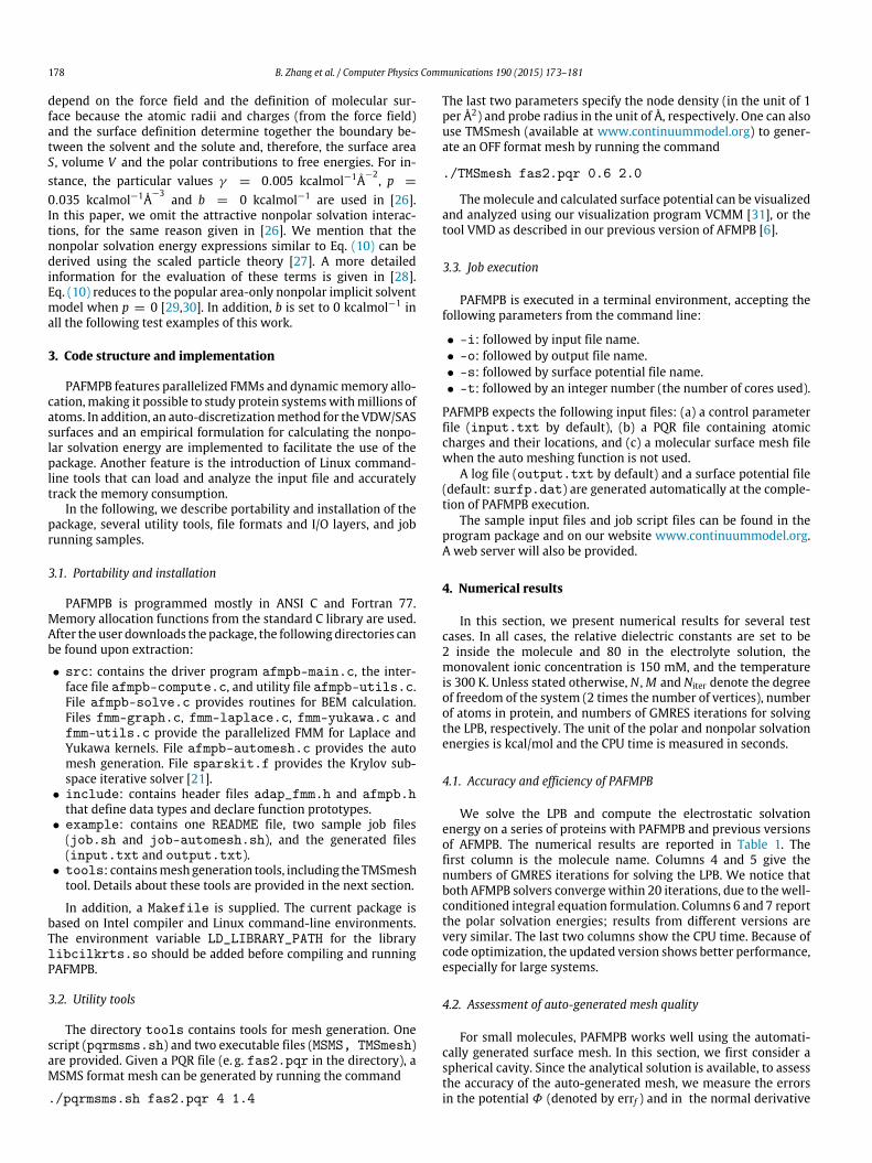
4.3. Parallel efficiency

To study the speedup factor from parallelization, PAFMPB istested on FasII, a 68-residue protein at various mesh resolutions.We list the CPU times and memory requirement using differentnumber of cores. The simulations are performed on an eight-coredesktop workstation with an Intel Xeon CPU @2.44 GHz and 48 GBmemory. Table 4 displays the memory requirement and iterations.Fig. 1 shows the speedup for different cores.

In Table 4, the numbers of vertices, hence the mesh density, isapproximately doubled each time. The solvation energies are ap-proaching the value at the largest density. When the degrees offreedom (column 1) increase, the numbers of iterations (column 3)are not increasing. From Table 4 and Fig. 1(a), the memory and av-erage CPU time per GMRES iteration scale almost linearly with thedegrees of freedom. From Fig. 1(b), a parallel efficiency of morethan 94% is achieved when using 4 cores and 86% when using 8cores.

We present next, parallel scalability results with the AChEmolecule data set. Table 5 displays the timing results in seconds.In this table, column 1 is the number of cores and column 2 is thetime to compute the geometrical mesh information used in ‘‘node-patch’’ method. Column 3 is the time for computing the polar sol-vation energy by FMM calls. Column 4 is the time for computingthe right hand side of Eq. (4). Column 5 is the time for assemblingthematrix. Columns 6 and 7 are for the near-field and far-field (us-ing FMM) matrix–vector products, respectively. The last columndisplays the total time for running the program. The most time-consuming part (more than three fourths of the total CPU timecost) is the far-field integration. The energy calculation, matrix as-sembly, and near-field integration also consume considerable CPUtime. Most of these parts have good parallel scalability. The mesh

Table 3

Comparison of number of GMRES iterations and energy results from auto generated meshes (VDW surface) andMSMSmeshes from different probe radius. Rp denotes proberadius.Auto-generated meshes MSMS meshesN Niter Ep Enp(VDW) Rp(N) Niter Ep Enp

416 6 �4.47 1.40 1.40(820) 6 �4.52 2.93876 7 �4.43 2.32 0.10(947) 8 �4.46 2.88

1762 7 �4.38 2.45 0.05(965) 6 �4.42 2.883529 7 �4.32 2.97 0.00(825) 6 �4.34 2.94

180 B. Zhang et al. / Computer Physics Communications 190 (2015) 173–181

Fig. 1. Parallel performance of PAFMPB applied to molecule FasII. (a) Total CPU time for one GMRES iteration step as a function of mesh size. (b) Speedup for differentnumber of cores using different mesh sizes (using the performance of one core as a reference).

Table 5

CPU times for main functions in PAFMPB for molecule AChE. (8280 atoms and 427064 elements, MSMS meshes were used).

cores Tgeometry Tenergy Trh TA Tnear Tfar Ttotal

1 0.36 69.74 5.24 42.87 38.01 534.30 694.022 0.31 36.31 2.73 22.65 19.66 277.05 362.124 0.28 18.47 1.41 12.26 10.18 139.28 185.438 0.26 9.92 0.75 13.26 5.48 72.76 105.78

Fig. 2. Auto generated triangular (at two poles) and quadrilateral elements for atwo-atom system.

geometry and mesh generation parts have poor scalability in ourcurrent code; however, their CPU time is negligible compared toother parts. We are currently studying effective ways to parallelizethe geometry related parts and the matrix assembly.

4.4. Large molecular system

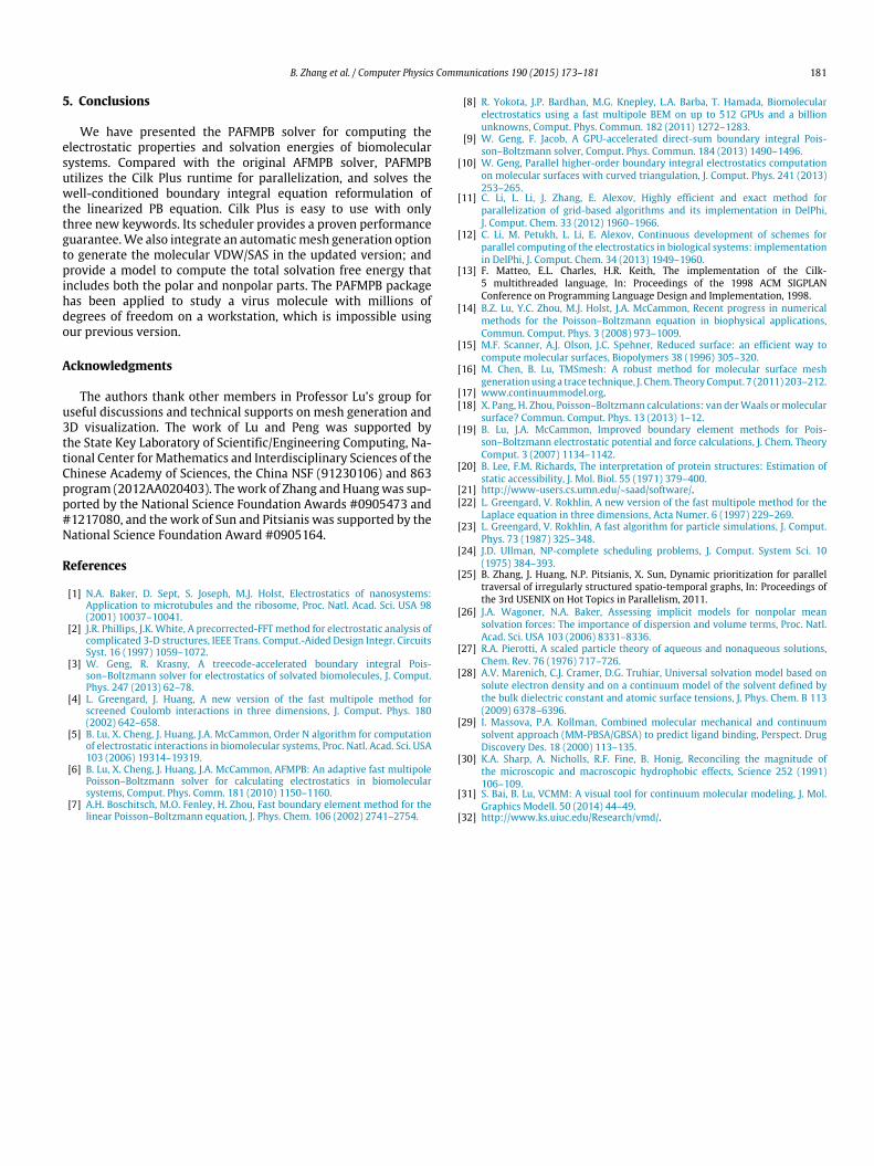
The previous AFMPB [6] is limited to the simulation of mediumsize molecules. PAFMPB uses a dynamic memory allocation tech-nique, and efficiently simulates larger macromolecules such as thedengue virus which consists of 1082160 atoms. In our simulation,we use the TMSmesh to obtain a mesh that has 19502784 ele-ments and 9758426 vertices. Since this mesh exceeds thememorycapacity of themachine used for scaling test, the calculation is per-formed on an Intel Xeon X7550 machine with 2.00 GHz and 1 TBmemory. PAFMPB solver terminates and output result after 70GM-RES iterations in 39117 s using 2 cores. Fig. 3(b) shows the surfacepotential obtained with the PAFMPB.

4.5. Visualization

The package VCMM (visual tool for continuum molecularmodeling), developed by Bai and Lu [31], can be convenientlyused with PAFMPB package to visualize and analyze the surfacemesh and numerical results. The output data formats for meshand surface potential files from PAFMPB can be directly adoptedby VCMM. Figs. 2 and 3 are produced by VCMM. Alternatively,VMD [32] can be applied for visualizing the simulation results [6].

Fig. 3. Visualization of a dengue virus system using VCMM [31]. (a) A surface mesh computed by TMSmesh consists of 19502784 elements and 9758426 vertices. (b)Surface potentials. Color bar is in unit of kcal/mol.ec .

B. Zhang et al. / Computer Physics Communications 190 (2015) 173–181 181

5. Conclusions

We have presented the PAFMPB solver for computing theelectrostatic properties and solvation energies of biomolecularsystems. Compared with the original AFMPB solver, PAFMPButilizes the Cilk Plus runtime for parallelization, and solves thewell-conditioned boundary integral equation reformulation ofthe linearized PB equation. Cilk Plus is easy to use with onlythree new keywords. Its scheduler provides a proven performanceguarantee.We also integrate an automaticmesh generation optionto generate the molecular VDW/SAS in the updated version; andprovide a model to compute the total solvation free energy thatincludes both the polar and nonpolar parts. The PAFMPB packagehas been applied to study a virus molecule with millions ofdegrees of freedom on a workstation, which is impossible usingour previous version.

Acknowledgments

The authors thank other members in Professor Lu’s group foruseful discussions and technical supports on mesh generation and3D visualization. The work of Lu and Peng was supported bythe State Key Laboratory of Scientific/Engineering Computing, Na-tional Center forMathematics and Interdisciplinary Sciences of theChinese Academy of Sciences, the China NSF (91230106) and 863program (2012AA020403). Thework of Zhang and Huangwas sup-ported by the National Science Foundation Awards #0905473 and#1217080, and the work of Sun and Pitsianis was supported by theNational Science Foundation Award #0905164.

References

[1] N.A. Baker, D. Sept, S. Joseph, M.J. Holst, Electrostatics of nanosystems:Application to microtubules and the ribosome, Proc. Natl. Acad. Sci. USA 98(2001) 10037–10041.

[2] J.R. Phillips, J.K. White, A precorrected-FFT method for electrostatic analysis ofcomplicated 3-D structures, IEEE Trans. Comput.-Aided Design Integr. CircuitsSyst. 16 (1997) 1059–1072.

[3] W. Geng, R. Krasny, A treecode-accelerated boundary integral Pois-son–Boltzmann solver for electrostatics of solvated biomolecules, J. Comput.Phys. 247 (2013) 62–78.

[4] L. Greengard, J. Huang, A new version of the fast multipole method forscreened Coulomb interactions in three dimensions, J. Comput. Phys. 180(2002) 642–658.

[5] B. Lu, X. Cheng, J. Huang, J.A. McCammon, Order N algorithm for computationof electrostatic interactions in biomolecular systems, Proc. Natl. Acad. Sci. USA103 (2006) 19314–19319.

[6] B. Lu, X. Cheng, J. Huang, J.A. McCammon, AFMPB: An adaptive fast multipolePoisson–Boltzmann solver for calculating electrostatics in biomolecularsystems, Comput. Phys. Comm. 181 (2010) 1150–1160.

[7] A.H. Boschitsch, M.O. Fenley, H. Zhou, Fast boundary element method for thelinear Poisson–Boltzmann equation, J. Phys. Chem. 106 (2002) 2741–2754.

[8] R. Yokota, J.P. Bardhan, M.G. Knepley, L.A. Barba, T. Hamada, Biomolecularelectrostatics using a fast multipole BEM on up to 512 GPUs and a billionunknowns, Comput. Phys. Commun. 182 (2011) 1272–1283.

[9] W. Geng, F. Jacob, A GPU-accelerated direct-sum boundary integral Pois-son–Boltzmann solver, Comput. Phys. Commun. 184 (2013) 1490–1496.

[10] W. Geng, Parallel higher-order boundary integral electrostatics computationon molecular surfaces with curved triangulation, J. Comput. Phys. 241 (2013)253–265.

[11] C. Li, L. Li, J. Zhang, E. Alexov, Highly efficient and exact method forparallelization of grid-based algorithms and its implementation in DelPhi,J. Comput. Chem. 33 (2012) 1960–1966.

[12] C. Li, M. Petukh, L. Li, E. Alexov, Continuous development of schemes forparallel computing of the electrostatics in biological systems: implementationin DelPhi, J. Comput. Chem. 34 (2013) 1949–1960.

[13] F. Matteo, E.L. Charles, H.R. Keith, The implementation of the Cilk-5 multithreaded language, In: Proceedings of the 1998 ACM SIGPLANConference on Programming Language Design and Implementation, 1998.

[14] B.Z. Lu, Y.C. Zhou, M.J. Holst, J.A. McCammon, Recent progress in numericalmethods for the Poisson–Boltzmann equation in biophysical applications,Commun. Comput. Phys. 3 (2008) 973–1009.

[15] M.F. Scanner, A.J. Olson, J.C. Spehner, Reduced surface: an efficient way tocompute molecular surfaces, Biopolymers 38 (1996) 305–320.

[16] M. Chen, B. Lu, TMSmesh: A robust method for molecular surface meshgenerationusing a trace technique, J. Chem. Theory Comput. 7 (2011) 203–212.

[17] www.continuummodel.org.[18] X. Pang, H. Zhou, Poisson–Boltzmann calculations: van derWaals ormolecular

surface? Commun. Comput. Phys. 13 (2013) 1–12.[19] B. Lu, J.A. McCammon, Improved boundary element methods for Pois-

son–Boltzmann electrostatic potential and force calculations, J. Chem. TheoryComput. 3 (2007) 1134–1142.

[20] B. Lee, F.M. Richards, The interpretation of protein structures: Estimation ofstatic accessibility, J. Mol. Biol. 55 (1971) 379–400.

[21] http://www-users.cs.umn.edu/~saad/software/.[22] L. Greengard, V. Rokhlin, A new version of the fast multipole method for the

Laplace equation in three dimensions, Acta Numer. 6 (1997) 229–269.[23] L. Greengard, V. Rokhlin, A fast algorithm for particle simulations, J. Comput.

Phys. 73 (1987) 325–348.[24] J.D. Ullman, NP-complete scheduling problems, J. Comput. System Sci. 10

(1975) 384–393.[25] B. Zhang, J. Huang, N.P. Pitsianis, X. Sun, Dynamic prioritization for parallel

traversal of irregularly structured spatio-temporal graphs, In: Proceedings ofthe 3rd USENIX on Hot Topics in Parallelism, 2011.

[26] J.A. Wagoner, N.A. Baker, Assessing implicit models for nonpolar meansolvation forces: The importance of dispersion and volume terms, Proc. Natl.Acad. Sci. USA 103 (2006) 8331–8336.

[27] R.A. Pierotti, A scaled particle theory of aqueous and nonaqueous solutions,Chem. Rev. 76 (1976) 717–726.

[28] A.V. Marenich, C.J. Cramer, D.G. Truhiar, Universal solvation model based onsolute electron density and on a continuum model of the solvent defined bythe bulk dielectric constant and atomic surface tensions, J. Phys. Chem. B 113(2009) 6378–6396.

[29] I. Massova, P.A. Kollman, Combined molecular mechanical and continuumsolvent approach (MM-PBSA/GBSA) to predict ligand binding, Perspect. DrugDiscovery Des. 18 (2000) 113–135.

[30] K.A. Sharp, A. Nicholls, R.F. Fine, B. Honig, Reconciling the magnitude ofthe microscopic and macroscopic hydrophobic effects, Science 252 (1991)106–109.

[31] S. Bai, B. Lu, VCMM: A visual tool for continuum molecular modeling, J. Mol.Graphics Modell. 50 (2014) 44–49.

[32] http://www.ks.uiuc.edu/Research/vmd/.