http://econ.geog.uu.nl/peeg/peeg.html

Papers in Evolutionary Economic Geography

# 16.26 Agglomeration economies: the heterogeneous contribution of

human capital and value chains

Dario Diodato, Frank Neffke, and Neave O'Clery

Agglomeration economies: the heterogeneous contribution of

human capital and value chains

Dario Diodato1, Frank Neffke2, and Neave O’Clery2

1Urban and Regional research center Utrecht (URU), Utrecht University - Heidelberglaan 2, 3584CS Utrecht,

The Netherlands2Center for International Development, Harvard University - 79 JFK street, 02138 Cambridge MA, USA

Abstract

We document the heterogeneity across sectors in the impact labor and input-output links

have on industry agglomeration. Exploiting the available degrees of freedom in coagglomeration

patterns, we estimate the industry-specific benefits of sharing labor needs and supply links with

local firms. On aggregate, coagglomeration patterns of services are at least as strongly driven by

input-output linkages as those of manufacturing, whereas labor linkages are much more potent

drivers of coagglomeration in services than in manufacturing. Moreover, the degree to which labor

and input-output linkages are reflected in an industry’s coagglomeration patterns is relevant for

predicting patterns of city-industry employment growth.

JEL classifications: J24, O14, R11

Keywords: Coagglomeration, Marshallian externalities, labor pooling, value chains, manufacturing,

services, regional diversification

Acknowledgments: Diodato acknowledges the financial support of NWO, Innovation Research Incentive Scheme

(VIDI). Project number: 45211013. The authors would like to thank Ron Boschma, Ricardo Hausmann, David

Rigby, Nicoletta Corrocher and the attendees at the Global Conference on Economic Geography 2015 in Oxford,

the Geography of Innovation 2016 conference in Toulouse and the CID Growth Lab seminar for their useful

comments and suggestions. Any mistake is our own.

1

1 Introduction

In spite of congestion, elevated factor costs and the risk that trade secrets leak to competitors, firms

of the same industry frequently locate close to each other (Ellison and Glaeser, 1999; Rosenthal and

Strange, 2001). The resulting agglomerations of firms in the same industry are often attributed to the

presence of three different types of externalities, namely the sharing of inputs, labor and knowledge.

However, there are good reasons to believe that different industries will benefit to different degrees

from agglomeration. Yet, the differential impact of agglomeration externalities for individual sectors of

the economy is still poorly understood. In this paper, we aim to assess the relative importance of two

major drivers of agglomeration across 120 different industries: the benefits of labor market pooling and

close proximity to value chain partners. In doing so, we also shed light on what drives agglomeration

in services, which, in spite of being the main employers in modern urban economies, are still relatively

understudied.

Marshall (1890) ascribed “the advantages which people following the same skilled trade get from near

neighborhood to one another” to three different types of agglomeration externalities: the benefits of a

large pool of skilled labor, easy access to local customers or suppliers and local knowledge spillovers.1

However, in spite of their early recognition and ample subsequent research, the relative importance

of each of these Marshallian externalities has fueled debate for over a century. A major obstacle,

termed ”Marshallian equivalence” by (Duranton and Puga, 2004), is the fact that all three Marshallian

agglomeration theories yield the same prediction for the spatial distribution of an industry: economic

establishments engaged in similar activities create benefits for one another that provide a rationale

for these establishments to agglomerate. This confluence of agglomeration benefits makes it hard to

determine which of them carries most weight as an explanation for the observed tendency of industries

to concentrate in space.

In a major stride forward Ellison, Glaeser and Kerr (2010), henceforth EGK, studied, not the agglom-

eration of individual industries, but the coagglomeration of pairs of industries. The rationale for this is

that industries that are similar along some dimensions, may differ along others. For instance, whereas

some industries will benefit from being colocated because they employ similar labor, other industries

may colocate because they maintain input-output or technological linkages. By analyzing the relation-

ship between locational similarity (coagglomeration) and similarity based on individual Marshallian

channels for industry pairs, EGK show that all three Marshallian externalities play a significant role.

On average, however, the most important explanation for why industries coagglomerate is input-output

linkages, closely followed by the sharing of labor. The weakest determinant of coagglomeration in EGK

is the potential for knowledge spillovers between two industries.

1Whereas theoretical models tend to divide agglomeration externalities into benefits of sharing, matching and learningin local economies Duranton and Puga (2004), most of the empirical literature on the topic categorizes Marshallianexternalities as economies in transportation, coordination or communication when acquiring one of three factors: labor,(intermediate) capital goods and knowledge.

2

However, such averages conceal marked differences across industries. For instance, whereas making

musical instruments requires years of on-the-job training of highly specialized workers, food-processing

often employs workers through temporary work agencies on short-term contracts, without much regard

for skills. Similarly, whereas car manufacturers often closely collaborate with their local suppliers

(Morgan and Cooke, 1998), the principal inputs for steel mills, coal and iron ore, are acquired on

anonymous exchanges with little need for interaction with suppliers. And finally, although knowledge

spillovers may be important drivers behind the clustering of biotechnology firms (Zucker et al., 1994),

they are less important in industries where technology progresses less rapidly. Meta-studies reviewing

the empirical literature on agglomeration externalities since the foundational papers by Glaeser et al.

(1992) and Henderson et al. (1995) confirm the existence of considerable variation in empirical findings

(Beaudry and Schiffauerova, 2009; Groot et al., 2015). We expect these differences to be driven in

part by variations across industries in how much they benefit from different types of Marshallian

externalities.2

In this paper we build on the work of EGK to explore whether the heterogeneity in agglomeration

benefits is expressed in the coagglomeration patterns of pairs of industries. While staying close to

the EGK framework, we deviate from it in two important respects. First, we do not control for

natural advantages, and second, we focus on externalities that arise from labor market pooling and

local input-output linkages, but ignore technological linkages. See Section 2.3 for a discussion of these

choices.

The paper is set up as follows. We first replicate key parts of the original work by EGK, which was

based on US manufacturing industries in the late 1980s and 1990s, using similar data for the 2000s.

Mimicking EGK, we do so using both Ordinary Least Squares (OLS) estimation and Instrumental

Variables (IV) based strategies that instrument labor and input-output linkages among US industries

by analogous measures constructed from data on the Mexican economy. As a second step, we extend

the analysis to include other industries, particularly in the services sector, while still excluding primary

sector industries and industries that purely cater to the needs of the local population (such as retail

activities and hospitals). In a third step, we relax the assumption that agglomeration effects are

homogeneous across industries fully and estimate the sensitivity of coagglomeration patterns to a

given agglomeration externality type for each industry separately.

In a final section, we explore whether the estimated differences in coagglomeration forces can help

predict local industry growth patterns. The empirical exercise in this section is related to work by

Dauth (2010), who studies how different agglomeration channels affect the growth of local industries,

the literature in economic geography on clusters (Porter, 2003; Delgado et al., 2010) and an emerging

literature on related diversification (Neffke et al., 2011; Hausmann et al., 2014). Although all these

2The Marshallian externalities reported in the before-mentioned meta-studies vary from significantly negative tosignificantly positive. The authors of these meta-studies attribute these divergent findings to a variety of factors, such asthe geographical area studied and methodological choices. Beaudry and Schiffauerova (2009) find that sectoral differencesmatter as well, although their study does not identify these as the main reason for the observed differences.

3

strands of research acknowledge the relevance of different types of inter-industry linkages, little is

known about their relative importance in the diversification and growth of local economies.

Confirming the results of EGK, we find that labor linkages and input-output linkages are more or

less equally important explanations for coagglomeration. This result holds not only when we replicate

their analysis for the manufacturing sector, but also when we extend it to include other sectors,

notably services. However, there are good reasons to expect coagglomeration tendencies in services

to be different from those in manufacturing. First of all, unlike manufactured goods, services are

often hard to trade over large distances. Consequently, services industries will need to colocate with

their customers. Second, services tend to be labor intensive and, moreover, the quality of services

often depends crucially on the quality of face-to-face interactions between a firm’s employees and

its customers (see for instance Kolko 1999 on the importance of agglomeration in services). Both

factors should augment the importance of access to adequate human capital. Taken together, these

considerations suggest that value chain and labor market pooling links should be particularly important

for coagglomeration patterns in services. This conjecture is confirmed when we consider manufacturing

and services separately. OLS effects of input-output linkages on coagglomeration are at least as large

in services as in manufacturing and the impact of labor externalities on coagglomeration patterns

of services is stronger than on those of manufacturing industries. When we allow full heterogeneity

in impacts across industries, we observe an even wider variation in effects. For some manufacturing

industries, coagglomeration with other industries can neither be attributed to labor nor to input-output

linkages. Typical examples are industries in furniture and food production. In other manufacturing

industries, such as machinery industries, coagglomeration patterns seem to be driven entirely by input-

output linkages. Coagglomeration rationales in services are even more heterogenous. Some industries,

like those in arts and culture cluster along both externality channels. In contrast, for media and

knowledge intensive business services, the possibility to pool labor dominates coagglomeration, whereas

the main driver of coagglomeration patterns in machinery repair services seems to be a desire to locate

close to value-chain partners.

Finally, we propose that the estimated effect-heterogeneity can help gauge an industry’s sensitivity

to the corresponding type of agglomeration benefits. For example, if a firm is active in an industry

that displays a strong dependence on specific labor and skills, then locating close to many other firms

sharing its labor needs will be highly beneficial. Conversely, choosing to locate near other firms with

similar value chain requirements will have less of an impact. We show this by predicting local industry

growth rates from the amount of local employment in industries that are connected by either value

chains or labor pooling linkages. Next, we interact these indicators of related local employment with

the sensitivity to labor pooling and value chains industries exhibit in their coagglomeration patterns.

Our estimates show that the sensitivity to input-output links determines how strongly a local industry’s

growth rates are affected by a strong local presence of industries to which it is linked in the value chain.

Similar, though somewhat less robust, effects are observed for labor market linkages.

Our main contribution is to highlight the variation of agglomeration forces across industries within a

4

unified analysis. Although the heterogeneity in agglomeration effects is widely acknowledged (Rosen-

thal and Strange, 2004; Beaudry and Schiffauerova, 2009; Groot et al., 2015; Rigby and Brown, 2015)

ours is the first paper, to our knowledge, to exploit coagglomeration to measure industry heterogeneity.

We find that coagglomeration of services is strongly driven by labor market pooling dynamics and,

in some of our specifications, also by value chain linkages. Given services’ importance as a driver of

urban growth, and against a background of secular decline in manufacturing, these results underscore

the importance of cities for the development of a strong service economy. The paper also contributes

to the growing literature of regional diversification (Delgado et al., 2010; Neffke et al., 2011; Hausmann

et al., 2014) by introducing industrial heterogeneity and asymmetry in the growth and diversification

process.

2 Methodology

2.1 Data

Our main datasets describe employment by region-industry pair in the US and Mexico. Geographical

employment patterns in the US are derived from the County Business Patterns (CBP) for the years

2003 and 2008.3 . Employment data for Mexico are taken from the economic censuses in 2003 and

2008. The analysis is carried out at three different levels of geographical aggregation: US counties (of

which there are 3,190), cities (939 metropolitan areas) and states (51). In Mexico our geographical

units are 2,455 municipalities, 58 cities (metropolitan areas) and 32 states. We will focus the discussion

on the results for metropolitan areas (labelled ’cities’ hereafter) as the most appropriate spatial unit

for defining labor markets and economically integrated regions. For the main results we also report

the outcome at county and state level as additional supporting evidence.

Unlike EGK, whose industries follow the Standard Industrial Classification (SIC87), in our paper,

industries are classified according to the North American Industry Classification System (NAICS).

Unfortunately, although the Mexican classification systems are also based on the NAICS, they are

not fully harmonized with those in the US. Starting from 317 4-digit US NAICS codes, we, therefore,

aggregate industries where necessary and create a new composite industry classification consisting of

215 distinct industries. After dropping industries for which we lack data to construct all covariates

used in this paper, there are 184 industries left. We restrict our sample further by dropping industries

for which their spatial distribution is strongly driven by the distribution of population. Examples

are retail, auto repair, construction and elementary schools. Note that we do not exclude extractive

activities such as mining. Although these activities are obviously restricted in their location choice, it

is still informative to see which other industries choose to locate in their vicinity. Following this logic

3CBP has different degrees of censoring depending on the geographical level of the data. To attribute a value ofemployment to a class we follow Holmes and Stevens (2004) For more details, we refer to Appendix D.

5

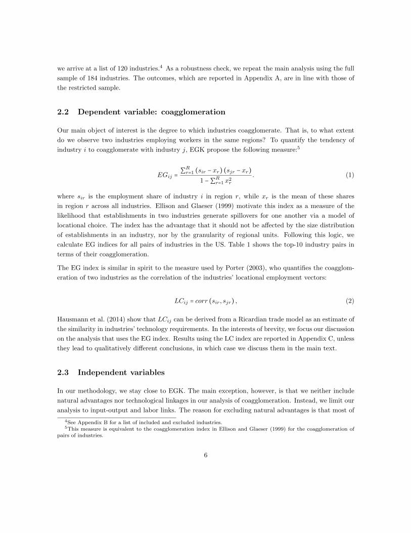
we arrive at a list of 120 industries.4 As a robustness check, we repeat the main analysis using the full

sample of 184 industries. The outcomes, which are reported in Appendix A, are in line with those of

the restricted sample.

2.2 Dependent variable: coagglomeration

Our main object of interest is the degree to which industries coagglomerate. That is, to what extent

do we observe two industries employing workers in the same regions? To quantify the tendency of

industry i to coagglomerate with industry j, EGK propose the following measure:5

EGij =∑Rr=1 (sir − xr) (sjr − xr)

1 −∑Rr=1 x

2r

. (1)

where sir is the employment share of industry i in region r, while xr is the mean of these shares

in region r across all industries. Ellison and Glaeser (1999) motivate this index as a measure of the

likelihood that establishments in two industries generate spillovers for one another via a model of

locational choice. The index has the advantage that it should not be affected by the size distribution

of establishments in an industry, nor by the granularity of regional units. Following this logic, we

calculate EG indices for all pairs of industries in the US. Table 1 shows the top-10 industry pairs in

terms of their coagglomeration.

The EG index is similar in spirit to the measure used by Porter (2003), who quantifies the coagglom-

eration of two industries as the correlation of the industries’ locational employment vectors:

LCij = corr (sir, sjr) , (2)

Hausmann et al. (2014) show that LCij can be derived from a Ricardian trade model as an estimate of

the similarity in industries’ technology requirements. In the interests of brevity, we focus our discussion

on the analysis that uses the EG index. Results using the LC index are reported in Appendix C, unless

they lead to qualitatively different conclusions, in which case we discuss them in the main text.

2.3 Independent variables

In our methodology, we stay close to EGK. The main exception, however, is that we neither include

natural advantages nor technological linkages in our analysis of coagglomeration. Instead, we limit our

analysis to input-output and labor links. The reason for excluding natural advantages is that most of

4See Appendix B for a list of included and excluded industries.5This measure is equivalent to the coagglomeration index in Ellison and Glaeser (1999) for the coagglomeration of

pairs of industries.

6

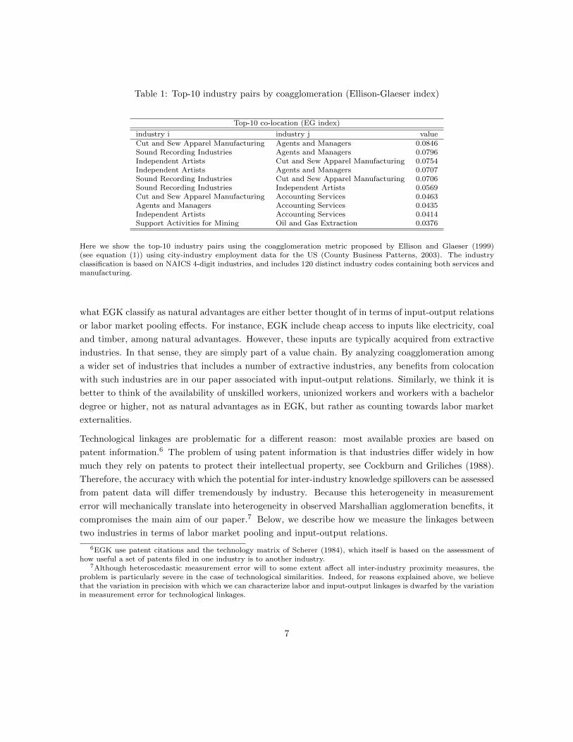
Table 1: Top-10 industry pairs by coagglomeration (Ellison-Glaeser index)

Top-10 co-location (EG index)

industry i industry j valueCut and Sew Apparel Manufacturing Agents and Managers 0.0846Sound Recording Industries Agents and Managers 0.0796Independent Artists Cut and Sew Apparel Manufacturing 0.0754Independent Artists Agents and Managers 0.0707Sound Recording Industries Cut and Sew Apparel Manufacturing 0.0706Sound Recording Industries Independent Artists 0.0569Cut and Sew Apparel Manufacturing Accounting Services 0.0463Agents and Managers Accounting Services 0.0435Independent Artists Accounting Services 0.0414Support Activities for Mining Oil and Gas Extraction 0.0376

Here we show the top-10 industry pairs using the coagglomeration metric proposed by Ellison and Glaeser (1999)(see equation (1)) using city-industry employment data for the US (County Business Patterns, 2003). The industryclassification is based on NAICS 4-digit industries, and includes 120 distinct industry codes containing both services andmanufacturing.

what EGK classify as natural advantages are either better thought of in terms of input-output relations

or labor market pooling effects. For instance, EGK include cheap access to inputs like electricity, coal

and timber, among natural advantages. However, these inputs are typically acquired from extractive

industries. In that sense, they are simply part of a value chain. By analyzing coagglomeration among

a wider set of industries that includes a number of extractive industries, any benefits from colocation

with such industries are in our paper associated with input-output relations. Similarly, we think it is

better to think of the availability of unskilled workers, unionized workers and workers with a bachelor

degree or higher, not as natural advantages as in EGK, but rather as counting towards labor market

externalities.

Technological linkages are problematic for a different reason: most available proxies are based on

patent information.6 The problem of using patent information is that industries differ widely in how

much they rely on patents to protect their intellectual property, see Cockburn and Griliches (1988).

Therefore, the accuracy with which the potential for inter-industry knowledge spillovers can be assessed

from patent data will differ tremendously by industry. Because this heterogeneity in measurement

error will mechanically translate into heterogeneity in observed Marshallian agglomeration benefits, it

compromises the main aim of our paper.7 Below, we describe how we measure the linkages between

two industries in terms of labor market pooling and input-output relations.

6EGK use patent citations and the technology matrix of Scherer (1984), which itself is based on the assessment ofhow useful a set of patents filed in one industry is to another industry.

7Although heteroscedastic measurement error will to some extent affect all inter-industry proximity measures, theproblem is particularly severe in the case of technological similarities. Indeed, for reasons explained above, we believethat the variation in precision with which we can characterize labor and input-output linkages is dwarfed by the variationin measurement error for technological linkages.

7

Input-output links

Value chains allow individual firms to specialize. However, such specialization also creates costs:

intermediates need to be shipped between firms and innovation efforts must be coordinated with

suppliers (Richardson, 1972; Abdel-Rahman, 1996; Porter, 1998). Because the costs of transportation

and coordination typically rise with distance, the coagglomeration of different parts of a value chain

can be an effective cost-reduction strategy.

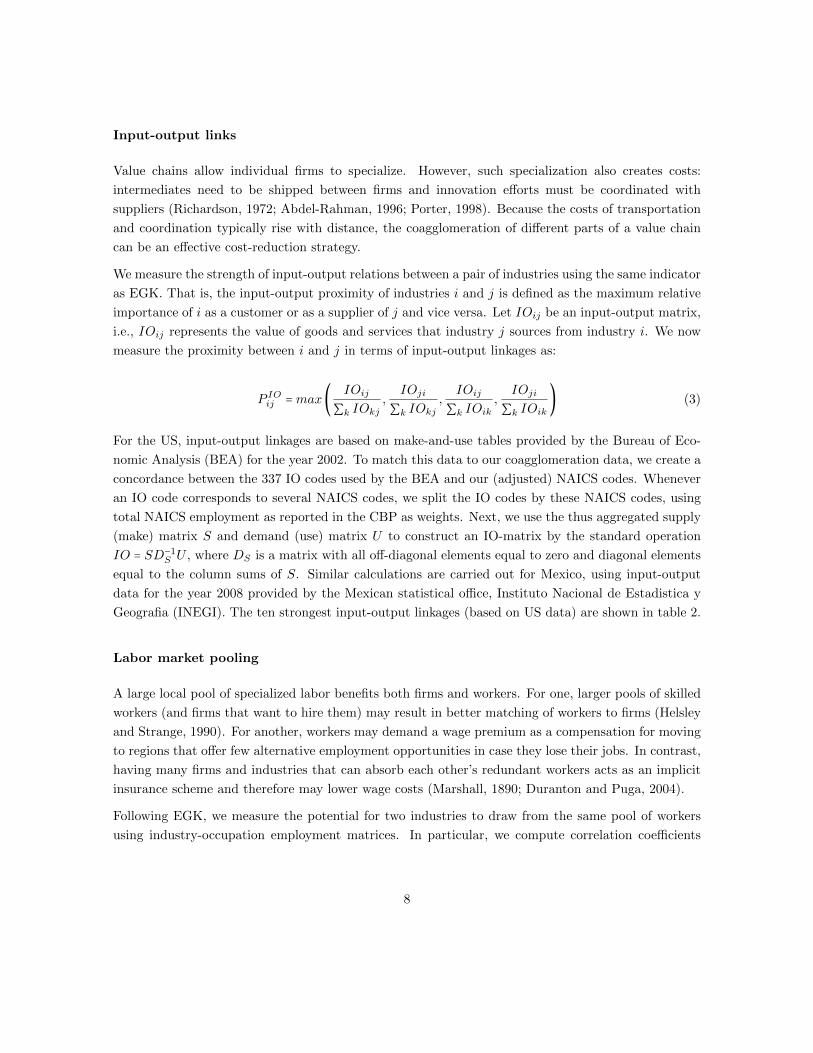
We measure the strength of input-output relations between a pair of industries using the same indicator

as EGK. That is, the input-output proximity of industries i and j is defined as the maximum relative

importance of i as a customer or as a supplier of j and vice versa. Let IOij be an input-output matrix,

i.e., IOij represents the value of goods and services that industry j sources from industry i. We now

measure the proximity between i and j in terms of input-output linkages as:

P IOij =max(IOij

∑k IOkj,

IOji

∑k IOkj,

IOij

∑k IOik,

IOji

∑k IOik) (3)

For the US, input-output linkages are based on make-and-use tables provided by the Bureau of Eco-

nomic Analysis (BEA) for the year 2002. To match this data to our coagglomeration data, we create a

concordance between the 337 IO codes used by the BEA and our (adjusted) NAICS codes. Whenever

an IO code corresponds to several NAICS codes, we split the IO codes by these NAICS codes, using

total NAICS employment as reported in the CBP as weights. Next, we use the thus aggregated supply

(make) matrix S and demand (use) matrix U to construct an IO-matrix by the standard operation

IO = SD−1S U , where DS is a matrix with all off-diagonal elements equal to zero and diagonal elements

equal to the column sums of S. Similar calculations are carried out for Mexico, using input-output

data for the year 2008 provided by the Mexican statistical office, Instituto Nacional de Estadistica y

Geografia (INEGI). The ten strongest input-output linkages (based on US data) are shown in table 2.

Labor market pooling

A large local pool of specialized labor benefits both firms and workers. For one, larger pools of skilled

workers (and firms that want to hire them) may result in better matching of workers to firms (Helsley

and Strange, 1990). For another, workers may demand a wage premium as a compensation for moving

to regions that offer few alternative employment opportunities in case they lose their jobs. In contrast,

having many firms and industries that can absorb each other’s redundant workers acts as an implicit

insurance scheme and therefore may lower wage costs (Marshall, 1890; Duranton and Puga, 2004).

Following EGK, we measure the potential for two industries to draw from the same pool of workers

using industry-occupation employment matrices. In particular, we compute correlation coefficients

8

Table 2: Top-10 industry pairs by strength of input-output links

Top-10 input-output links

industry i industry j valuePetroleum and Coal Manufacturing Oil and Gas Extraction 0.6776Other Apparel Manufacturing Cut and Sew Apparel Manufacturing 0.6001Leather and Hide Tanning Animal slaughtering and processing 0.5811Motor Vehicle Parts Manufacturing Motor Vehicle Manufacturing 0.5720Motor Vehicle Manufacturing Motor Vehicle Body Manufacturing 0.5351Pulp, Paper, and Paperboard Mills Paper Product Manufacturing 0.4617Support Activities for Mining Oil and Gas Extraction 0.4575Motor Vehicle Manufacturing Audio-Video Equipment Manufacturing 0.4343Spectator Sports Radio and Television Broadcasting 0.4269Motor Vehicle Parts Manufacturing Leather and Hide Tanning 0.4227

Here we show top-10 industry pairs in terms of input-output linkages, defined as the maximum relative importance ofone industry as a customer or as a supplier of the other and vice versa (see equation (3)), based on make-and-use tablesprovided by the US Bureau of Economic Analysis (BEA) for the year 2002.

across occupations between Eio and Ejo, where Eio represents the number of workers in occupation o

that are (nation-wide) employed by industry i:

PLij = corr(Eio,Ejo). (4)

For the US, we use industry-occupation data for the year 2002 as reported in the Occupational Em-

ployment Statistics (OES), while for Mexico, we use the Encuesta Nacional de Ocupacion y Empleo

(ENOE) for the year 2005.8 The ten strongest labor linkages (using US data) are reported in table 3.

2.4 Descriptive statistics

Excluding the diagonal, there are 7,140 unique industry pairs in our sample of 120 industries. Table 4

contains descriptive statistics for this sample. All variables have similar means in the US and Mexico.

However, it is interesting to note that, for all variables, the dispersion is larger in Mexico, and sometimes

substantially so. Although the greater dispersion in the Mexican variables may be structural, it could

also mean that the variables constructed from US data are measured more accurately.

Table 5 reports correlation coefficients between the various dependent and independent variables. The

Mexican and US versions of input-output and labor proximity measures are relatively highly correlated

8The US and Mexico use different classifications of occupations. This is, in principle, unproblematic, because indus-tries are still recorded in both sources according to the NAICS classification. However, because the ENOE uses a mixof 3- and 4-digit classes (consisting of 68 3-digit and 113 4-digit codes), we have to split some 3-digit industries in theENOE into 4-digit codes. Consequently, some industry pairs in Mexico are mechanically attributed the same PL valuesand somewhat under 3% of off-diagonal elements are equal to 1.

9

Table 3: Top-10 industry pairs by strength of labor links

Top-10 labor links

industry i industry j valueOther Textile Product Mills Other Apparel Manufacturing 0.9919Other Apparel Manufacturing Cut and Sew Apparel Manufacturing 0.9885Other Textile Product Mills Cut and Sew Apparel Manufacturing 0.9805Other Transportation Equipment Agri/Construction/Mining Machinery 0.9802Motor Vehicle Parts Manufacturing Hardware Manufacturing 0.9766Other Transportation Equipment Motor Vehicle Body Manufacturing 0.9760Motor Vehicle Body Manufacturing Heating/Cooling Equipment 0.9756Other Machinery Manufacturing Agri/Construction/Mining Machinery 0.9742Household Appliance Manufacturing Hardware Manufacturing 0.9737Heating/Cooling Equipment Hardware Manufacturing 0.9715

Here we show top-10 industry pairs in terms of labor linkages, computed as a correlation of industry employment byoccupation (see equation (4)), and based industry-occupation data for the year 2002 as reported in the US OccupationalEmployment Statistics (OES).

Table 4: Summary statistics

Variable Obs Mean Std. Dev. Min Max

United States

EG index 7140 0.0001 0.0047 -0.0232 0.0846LC index 7140 0.7166 0.1209 0.4854 0.9915Input-output 7140 0.0124 0.0353 0.0000 0.6776Labor 7140 0.6013 0.0997 0.4956 0.9919

Mexico

EG index 7140 0.0005 0.0477 -0.2579 0.5149LC index 7140 0.7784 0.1657 0.4399 0.9994Input-output 7140 0.0143 0.0503 0.0000 1.0000Labor 7140 0.5565 0.1094 0.4828 1.0000

Here we provide summary data for coagglomeration (EG and LC metrics), input-output and labor linkages for 120 ∗(120 − 1)/2 = 7140 unique industry pairs for comparable data in both the US (top) and Mexico (bottom).

10

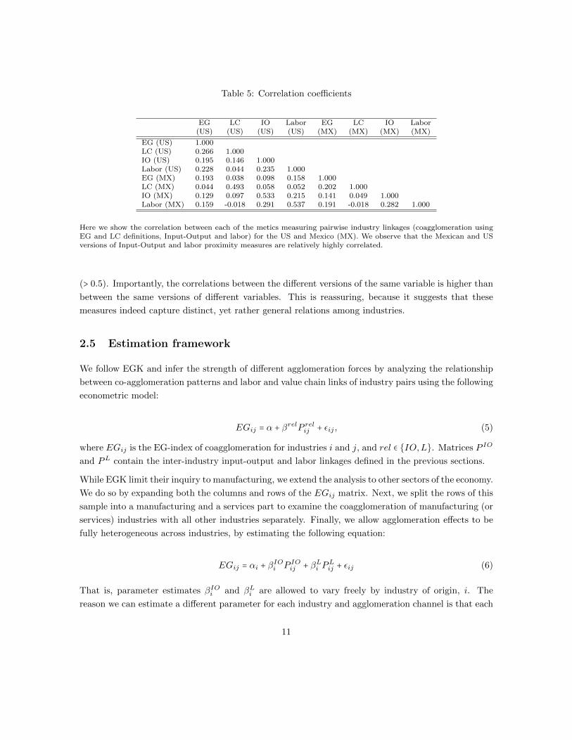
Table 5: Correlation coefficients

EG LC IO Labor EG LC IO Labor(US) (US) (US) (US) (MX) (MX) (MX) (MX)

EG (US) 1.000LC (US) 0.266 1.000IO (US) 0.195 0.146 1.000Labor (US) 0.228 0.044 0.235 1.000EG (MX) 0.193 0.038 0.098 0.158 1.000LC (MX) 0.044 0.493 0.058 0.052 0.202 1.000IO (MX) 0.129 0.097 0.533 0.215 0.141 0.049 1.000Labor (MX) 0.159 -0.018 0.291 0.537 0.191 -0.018 0.282 1.000

Here we show the correlation between each of the metics measuring pairwise industry linkages (coagglomeration usingEG and LC definitions, Input-Output and labor) for the US and Mexico (MX). We observe that the Mexican and USversions of Input-Output and labor proximity measures are relatively highly correlated.

(> 0.5). Importantly, the correlations between the different versions of the same variable is higher than

between the same versions of different variables. This is reassuring, because it suggests that these

measures indeed capture distinct, yet rather general relations among industries.

2.5 Estimation framework

We follow EGK and infer the strength of different agglomeration forces by analyzing the relationship

between co-agglomeration patterns and labor and value chain links of industry pairs using the following

econometric model:

EGij = α + βrelP relij + εij , (5)

where EGij is the EG-index of coagglomeration for industries i and j, and rel ∈ {IO,L}. Matrices P IO

and PL contain the inter-industry input-output and labor linkages defined in the previous sections.

While EGK limit their inquiry to manufacturing, we extend the analysis to other sectors of the economy.

We do so by expanding both the columns and rows of the EGij matrix. Next, we split the rows of this

sample into a manufacturing and a services part to examine the coagglomeration of manufacturing (or

services) industries with all other industries separately. Finally, we allow agglomeration effects to be

fully heterogeneous across industries, by estimating the following equation:

EGij = αi + βIOi P IOij + β

Li P

Lij + εij (6)

That is, parameter estimates βIOi and βLi are allowed to vary freely by industry of origin, i. The

reason we can estimate a different parameter for each industry and agglomeration channel is that each

11

industry can coagglomerate with all other industries. Consequently, there are 119 observations per

industry. Equation (6) can be estimated by running separate regressions for each i. However, it will be

more convenient to estimate the coefficients simultaneously using the following two-way fixed effects

model:9

EGij = αi + δj + βIOi P IOij + β

Li P

Lij + εij (7)

This procedure yields two vectors with estimates of industry-specific agglomeration effects, β̂IO and

β̂L. The elements of these vectors represent the extent to which input-output and labor market linkages

are expressed in an industry’s coagglomeration patterns.

A possible cause for concern is that P IOij and PLij are themselves endogenous. Accordingly, EGK argue

that OLS estimates may be upward-biased if the historical coagglomeration of two industries prompted

these industries to adjust their production technologies in such a way that they could use each other’s

outputs or skilled workers. Another concern is that P IOij and PLij are only imperfect proxies of the

degree to which industries can exchange products and labor. Such measurement error would lead

to a downward bias in our estimates. In line with EGK, we therefore also estimate the models in

equations (5) and (7) using on IV approach. As instruments, we use analogously constructed variables

based on Mexican data. Similar to the UK-based instruments in EGK, our instruments are valid, as

long as idiosyncratic patterns in the input-output and labor linkages in Mexico are uncorrelated with

coagglomeration patterns in the US.

3 Empirical findings

3.1 Replication of EGK results

We start our analysis of the impact of labor market pooling and input-output relations on coagglom-

eration assuming that the two factors have homogeneous effects across industries. Later we will relax

this assumption more and more. In the analysis below, we rescale all variables such that they are

expressed in units of standard deviations.

Table 6 first replicates the results of EGK, including manufacturing industries only.10 The table shows

the results of univariate OLS specifications in which the effect of labor pooling and value chain linkages

are estimated separately. The left part of the table (columns 1 to 3) shows our own estimates. For

9Moreover, in contrast to estimating separate equations for each industry, equation (7) allows the inclusion of bothindustry of origin and of destination fixed effects.

10For maximal comparability, manufacturing industries are here defined at the 4-digit level of the original US NAICSclassification. In all subsequent analysis, we use the NAICS classification that was harmonized with the Mexicanimplementation of NAICS.

12

Table 6: OLS univariate regressions (EGK replication)

EG index (our estimates) EG index (EGK estimates)

(1) (2) (3) (4) (5) (6)state city county state city county

Input-output 0.214 0.177 0.144 0.205 0.167 0.130(0.035) (0.032) (0.029) (0.037) (0.028) (0.022)

Observations 3655 3655 3655 7381 7381 7381R2 0.060 0.060 0.047 0.042 0.028 0.017

Labor 0.181 0.164 0.195 0.180 0.106 0.082(0.018) (0.018) (0.016) (0.014) (0.016) (0.013)

Observations 3655 3655 3655 7381 7381 7381R2 0.029 0.035 0.060 0.032 0.011 0.007

Robust standard errors in parentheses.

Columns 1-3 replicate the univariate regression results of Ellison, Glaeser and Kerr (2010) (shown in columns 4-6) usingequivalent data for the US from 2003 for manufacturing industries and three levels of spatial aggregation: states, citiesand counties. In all cases the dependent variable is the pairwise EG-based coagglomeration linkages, and the independentvariable is either the corresponding metric for value chain linkages or labor pooling (see equation (5)). Most of the newestimates are remarkably close to those of EGK despite the fact that the new sample refers to a different period and moreaggregate industry definitions: both externality channels are important and have similar impacts on coagglomeration.

convenience, the findings in the original paper by EGK (Table 3, p. 1204) are shown on the right

(columns 4 to 6).

In spite of the fact that our sample refers to a different period and more aggregate industry definitions

(manufacturing codes are less detailed at the 4-digit NAICS level than at the 3-digit SIC level), most

of our estimates are remarkably close to those of EGK: both externality channels are important and

have similar impacts on coagglomeration. The only substantive difference is that we find larger effects

of labor pooling at the city and county levels than EGK. As a consequence, our estimates imply that,

at the county level, labor pooling is a stronger determinant of coagglomeration than are input-output

links instead of vice versa.

3.2 Extended sample

The EGK results are derived only for manufacturing. Do conclusions change when we extend the

sample of industries? Using the (adjusted) NAICS classification, there are 83 manufacturing indus-

tries, which represent roughly two-thirds of the 120 industries in the overall sample. Consequently,

the number of observations rises to 7,140 (= 120(120−1)2

). Table 7 contains results of the estimations

for this extended sample. The first three columns report OLS estimates, columns 4 to 6 show IV

estimates, where US input-output proximity (P IOij ) and labor proximity (PLij ) are instrumented by

their counterparts constructed from Mexican data.

The OLS regressions show that, in the extended sample, value chain and labor market links are

13

Table 7: OLS and IV univariate regressions on extended sample

(1) (2) (3) (4) (5) (6)OLS OLS OLS IV IV IVstate city county state city county

EG index

Input-output 0.295 0.215 0.176 0.372 0.267 0.201(0.041) (0.025) (0.028) (0.045) (0.032) (0.032)

Observations 7140 7140 7140 7140 7140 7140R2 0.069 0.038 0.025 0.064 0.036 0.024

Labor 0.261 0.229 0.178 0.347 0.296 0.194(0.012) (0.011) (0.011) (0.031) (0.020) (0.018)

Observations 7140 7140 7140 7140 7140 7140R2 0.065 0.052 0.030 0.058 0.048 0.030

Robust standard errors in parentheses.

Idem table 6 but in this case we include all industries, not just manufacturing as in the previous table, for a total of 120industries. We show OLS results for the US (columns 1-3), and using IV estimates where US input-output proximity(P IO

ij ) and labor proximity (PLij ) are instrumented by their counterparts constructed from Mexican data (columns 4-6).

The regressions show that, in this extended sample, value chain and labor market links are even more important driversof coagglomeration than in the manufacturing only sample.

even more important drivers of coagglomeration than in the manufacturing sample. Focusing on the

city-level estimates, a one-standard-deviation increase in human capital similarities increases indus-

tries’ coagglomeration by 0.23 standard deviations. Similarly, a one-standard-deviation increase in

the strength of value-chain linkages between industries increases their coagglomeration index by 0.22

standard deviations. Turning to columns (4) to (6), we find that IV estimates significantly exceed

OLS estimates.11 The effect of a one-standard-deviation increase in the strength of value-chain links

increases coagglomeration tendencies by 0.27 standard deviations, whereas a similar increase in human

capital similarity increases coagglomeration by 0.30 standard deviations. The fact that IV estimates

are higher than OLS estimates is similar to what EGK report, although in EGK this is limited to

the effects of input-output linkages.12 It appears that reverse causality does not lead to a net overall

upward bias. Instead, our findings are consistent with the notion that inter-industry proximities are

measured with some error.

3.3 Manufacturing versus services

The fact that we find tendencies of industries to coagglomerate along both labor and IO channels

to increase as we extend our sample of industries suggests that these factors are stronger drivers of

11First-stage results (not reported) are very strong: the estimated effects of the instruments on endogenous variablesexhibit t-statistics of 42 for labor similarities and 8.6 for input-output linkages.

12For labor linkages, OLS and IV estimates are roughly equal in EGK.

14

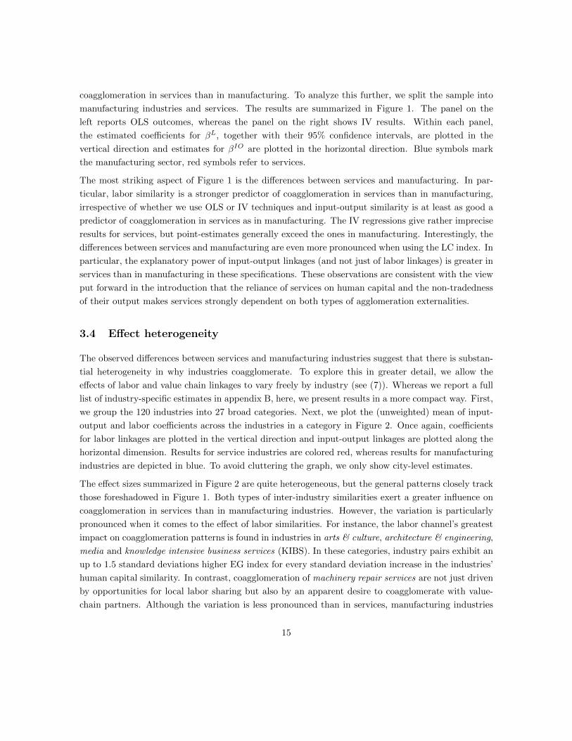
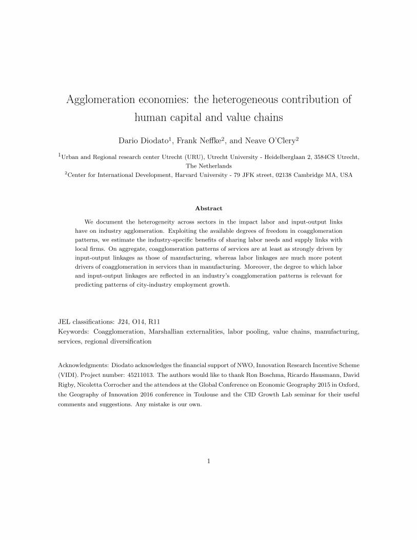
coagglomeration in services than in manufacturing. To analyze this further, we split the sample into

manufacturing industries and services. The results are summarized in Figure 1. The panel on the

left reports OLS outcomes, whereas the panel on the right shows IV results. Within each panel,

the estimated coefficients for βL, together with their 95% confidence intervals, are plotted in the

vertical direction and estimates for βIO are plotted in the horizontal direction. Blue symbols mark

the manufacturing sector, red symbols refer to services.

The most striking aspect of Figure 1 is the differences between services and manufacturing. In par-

ticular, labor similarity is a stronger predictor of coagglomeration in services than in manufacturing,

irrespective of whether we use OLS or IV techniques and input-output similarity is at least as good a

predictor of coagglomeration in services as in manufacturing. The IV regressions give rather imprecise

results for services, but point-estimates generally exceed the ones in manufacturing. Interestingly, the

differences between services and manufacturing are even more pronounced when using the LC index. In

particular, the explanatory power of input-output linkages (and not just of labor linkages) is greater in

services than in manufacturing in these specifications. These observations are consistent with the view

put forward in the introduction that the reliance of services on human capital and the non-tradedness

of their output makes services strongly dependent on both types of agglomeration externalities.

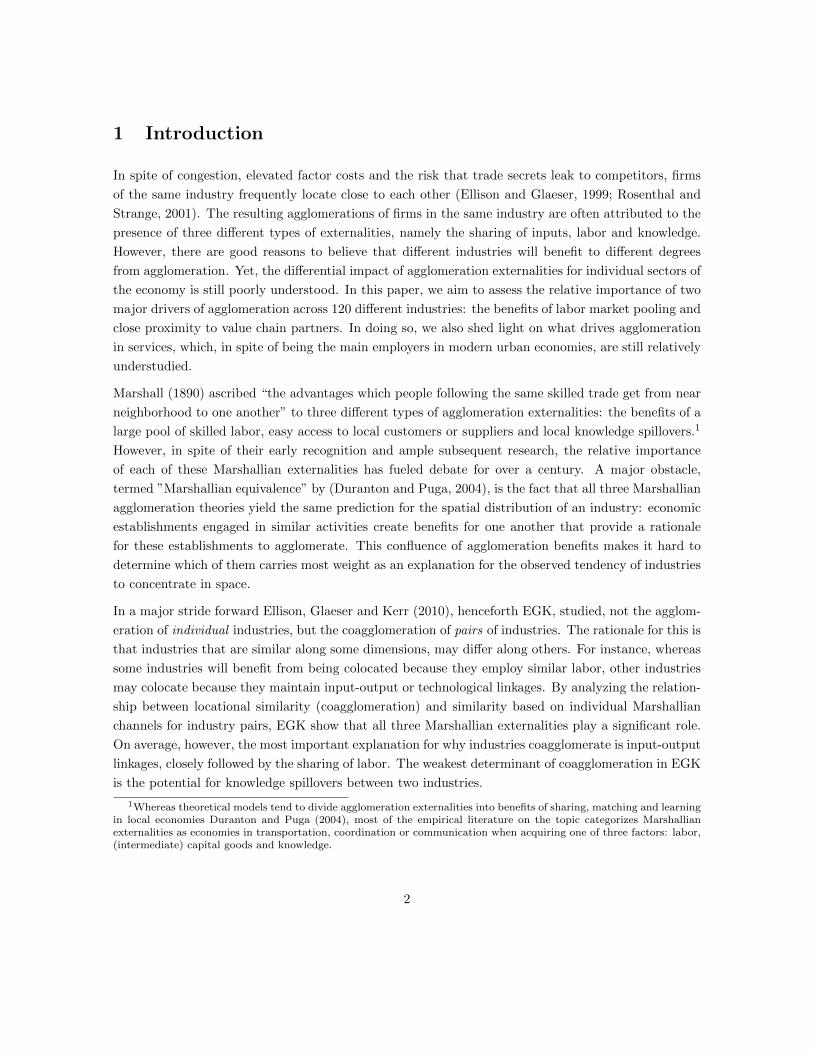
3.4 Effect heterogeneity

The observed differences between services and manufacturing industries suggest that there is substan-

tial heterogeneity in why industries coagglomerate. To explore this in greater detail, we allow the

effects of labor and value chain linkages to vary freely by industry (see (7)). Whereas we report a full

list of industry-specific estimates in appendix B, here, we present results in a more compact way. First,

we group the 120 industries into 27 broad categories. Next, we plot the (unweighted) mean of input-

output and labor coefficients across the industries in a category in Figure 2. Once again, coefficients

for labor linkages are plotted in the vertical direction and input-output linkages are plotted along the

horizontal dimension. Results for service industries are colored red, whereas results for manufacturing

industries are depicted in blue. To avoid cluttering the graph, we only show city-level estimates.

The effect sizes summarized in Figure 2 are quite heterogeneous, but the general patterns closely track

those foreshadowed in Figure 1. Both types of inter-industry similarities exert a greater influence on

coagglomeration in services than in manufacturing industries. However, the variation is particularly

pronounced when it comes to the effect of labor similarities. For instance, the labor channel’s greatest

impact on coagglomeration patterns is found in industries in arts & culture, architecture & engineering,

media and knowledge intensive business services (KIBS). In these categories, industry pairs exhibit an

up to 1.5 standard deviations higher EG index for every standard deviation increase in the industries’

human capital similarity. In contrast, coagglomeration of machinery repair services are not just driven

by opportunities for local labor sharing but also by an apparent desire to coagglomerate with value-

chain partners. Although the variation is less pronounced than in services, manufacturing industries

15

Figure 1: Coagglomeration effects, manufacturing versus services

citycounty

state

citycountystate

0.5

1β L

-.2 0 .2 .4 .6 .8

β IO

OLS

city

county

state

citycounty

state

0.5

1β L

-.2 0 .2 .4 .6 .8

β IO

IVEG-index

citycountystate

citycounty

state

0.5

1β L

-.2 0 .2 .4 .6 .8

β IO

OLS

citycountystate

citycounty

state

0.5

1β L

-.2 0 .2 .4 .6 .8

β IO

IVLC-index

The figures depict estimated labor pooling effects (vertical axis) and value chain effects (horizontal axis) from separate

estimations of equation (5) on the sample of services and manufacturing industries. Estimates for the coagglomeration

patterns of services are plotted using open, red markers, those for manufacturing industries using solid, blue markers.

State-level estimates are marked by squares, city-level estimates by triangles and municipality-level estimates by circles.

The crosshairs represent 95% confidence intervals based on robust standard errors. IV estimates use analogous variables

for labor pooling and input-output linkages using Mexican data.

16

display heterogeneous effects as well. For instance, the coagglomeration patterns of industries in

hardware and in machinery manufacturing follow value-chain as well as labor-pooling relations. In

contrast, pharma & medical industries tend to coagglomerate with customers or suppliers, but not

with industries that employ similar labor.

4 Marshallian Externalities and Regional Diversification

So far, we have used the EGK framework to show that the balance between labor market-pooling

and value-chain-based agglomeration externalities differs widely across industries. However the co-

agglomeration framework is static in nature. Do these differences manifest themselves in the spatial

dynamics of agglomeration? To explore this issue, we move to an analysis of industries’ growth paths

in a particular location, i.e., given an existing portfolio of industries. In doing so, we connect to a

large and growing literature that has focused on the role of Marshallian externalities in the evolution

of regions’ industrial structure. This literature suggests that inter-industry linkages are important for

understanding diversification processes, as regions branch into new economic activities that build on

existing strengths. Using this approach, industries have been found to grow faster in regions with

much employment in related industries (Porter, 2003; Greenstone et al., 2008; Delgado et al., 2010;

Neffke et al., 2011; Hausmann et al., 2014).

Yet most of this work implicitly assumes that all industries benefit equally from inter-industry spillovers.

Moreover, it typically captures relatedness through a single Marshallian channel. In this section, we

use the insights on industry-specific (co-)agglomeration externalities gained in the previous section, to

enhance the econometric models of local industry growth rates that have been used by authors in this

strand of the literature. To do so, let the relatedness between industries i and j be measured by one of

our two proximity measures P relij ∈ {PLij , PIOij }. We can now calculate the proximity-weighted (related)

employment for region-industry (i, r) in year t as:

Erelirt =∑

j

P relij

∑k≠i P relik

Ejrt.

This expression can be interpreted as the amount of related employment already present in the local

economy, where what we call “related” depends on rel. For example, in the case of labor ELirt represents

an index that reflects the size of the local workforce with skills and know-how that are relevant to

industry i.

Letting G03−08ir refer to the logarithm of employment growth of industry i in region r between 2003 and

2008, i.e., Gir = ln (Eir08) − ln (Eir03) and restricting the sample to all local industries with non-zero

17

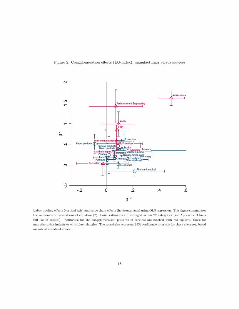
Figure 2: Coagglomeration effects (EG-index), manufacturing versus services

Extraction

Food

TobaccoTextileWood productsPaper products

PrintingPetroleum & Coal

Chemical

Pharma & medical

Materials

Mineral products

HardwareMachinery

Electronics

Electrical eqpt

Transportation eqptFurniture

Media

TelecommunicationIT services

Architecture & Engineering

KIBS

Education

Art & culture

Recreation

Machinery repair

-.50

.51

1.5

2β L

-.2 0 .2 .4 .6

β IO

Labor pooling effects (vertical axis) and value chain effects (horizontal axis) using OLS regression. This figure summarizes

the outcomes of estimations of equation (7). Point estimates are averaged across 27 categories (see Appendix B for a

full list of results). Estimates for the coagglomeration patterns of services are marked with red squares, those for

manufacturing industries with blue triangles. The crosshairs represent 95% confidence intervals for these averages, based

on robust standard errors.

18

employment in 2003,13 we estimate:

G03−08ir = δ ln (Eir03) + γ

rel ln (Erelir03) + ιi + ρr + εir03 (8)

where δ captures mean reversion effects, and ιi and ρr are industry and region dummies. The parameter

of interest, γrel, captures to what extent the growth in a local industry can be predicted from the

amount of related activity already present in the local economy.

Table 8 contains results when using cities as the spatial unit of analysis. In line with prior literature

(e.g., Delgado et al., 2010; Hausmann et al., 2014), we find significant and negative effects for the mean

reversion term δ and positive effects of γrel, regardless of whether we measure proximity in terms of

labor or input-output linkages. However, our findings so far suggest that the degree to which each of

these proximities matters will vary by industry. We, therefore, augment (8) by interacting the amount

of related employment in a city with β̂reli , our estimates for βIOi and βLi which contain information

on how important a proximity is to an industry. To facilitate interpretation, the β̂reli are expressed in

units of standard deviations from their respective mean. This yields the following equation:14

G03−08ir = δ ln (Eir03) + γ

rel ln (Erelir03) + γrelβ β̂reli ln (Erelir03) + ιi + ρr + εir03 (9)

If β̂reli captures any information on the importance of the corresponding agglomeration externality, we

would expect γrelβ to be positive. Table 8 shows that this is indeed the case.

The interaction effect, γrelβ , is always positive, but consistently statistically significant only when using

the industry-specific effects derived from regressions using the LC index of coagglomeration (columns

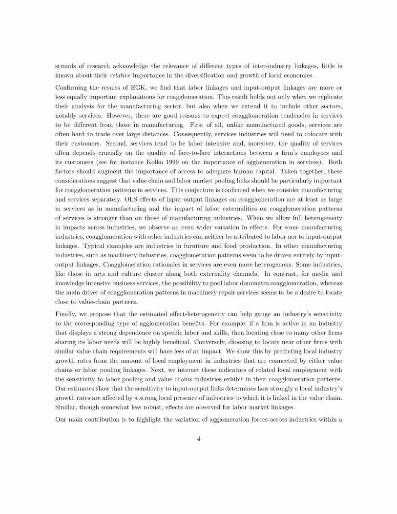
(5), (6) and (9)). The marginal effects of related employment are given by:

∂G03−08ir

∂Erelir

= γrel + γrelβ β̂reli .

Figure 3 plots these partial derivatives against β̂reli on a range that reflects the actual coefficient

estimates obtained in section 3.4. The strongest interaction effects are visible when using industry-

specific effects estimated in regression analysis based on the LC index. In these equations, elasticities

for value-chain related employment run from as low as 2% for some industries to as high as 4% for

others. The range of elasticities is even greater for employment related in terms of human-capital

similarities, starting from a low 4% for industries with coagglomeration patterns that are not very

sensitive to human capital similarities and reaching over 10% where such similarities are very strong

drivers of coagglomeration. The fact that the industry-specific coagglomeration effects derived in

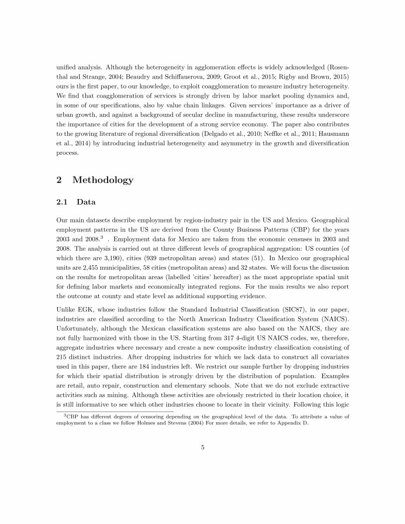
13In the appendix, we also show results for growth at the extensive margin, estimating the entry probability for localindustries that were non-existent in 2003. Conclusions derived from this analysis are similar to the ones presented here.

14Note that any level-effects of βreli will be absorbed in ιi.

19

Table 8: Growth in local industries

City-industry employment growth

(1) (2) (3) (4) (5) (6) (7) (8) (9)lnEir03 -0.1995 -0.2029 -0.1995 -0.2029 -0.1999 -0.2058 -0.2037 -0.2037 -0.2074

(0.0034) (0.0035) (0.0034) (0.0035) (0.0034) (0.0035) (0.0035) (0.0035) (0.0035)lnEIO

ir03 0.0280 0.0280 0.0285 0.0151 0.0152 0.0179(0.0045) (0.0045) (0.0045) (0.0046) (0.0046) (0.0046)

lnELir03 0.0612 0.0612 0.0602 0.0571 0.0571 0.0555

(0.0050) (0.0050) (0.0050) (0.0051) (0.0051) (0.0052)

lnEIOir03β̂

IOi,EG 0.0030 0.0024

(0.0021) (0.0021)

lnELir03β̂

Li,EG 0.0008 0.0008

(0.0020) (0.0020)

lnEIOir03β̂

IOi,LC 0.0070 0.0076

(0.0020) (0.0020)

lnELir03β̂

Li,LC 0.0234 0.0243

(0.0020) (0.0020)

Obs. 37835 37835 37835 37835 37835 37835 37835 37835 37835Adj.R2 0.1295 0.1325 0.1296 0.1325 0.1298 0.1343 0.1327 0.1327 0.1349

The dependent variable is the logarithm of growth of the employment in local industries between 2003 and 2008. Eir03

is the employment in industry i in city r in the year 2003. EIOir03 and EL

ir03 define the employment related to industry i

according to input-output linkages and labor linkages respectively, in region r in the year 2003. The terms EIOir03β̂

IOi,EG

and ELir03β̂

Li,EG refer to the interaction of related employment and the estimated industry-specific effects of input-output

linkages or labor linkages in the coagglomeration regressions. Industry-specific coagglomeration effects are centered on

their means and scaled by their standard deviations. All regressions include industry and region dummies. Robust

standard errors are reported in parentheses.

20

Section 3.4 are also reflected in industries’ local growth patterns does not just tell us something about

local industries’ growth patterns. It also raises our confidence in the estimated effect heterogeneity

itself.

5 Conclusion

Extending the work by Ellison, Glaeser and Kerr (2010) on why industries coagglomerate, we find

evidence of substantial heterogeneity across industries. Whereas in some industries, firms tend to locate

close to their value-chain partners, in others they tend to locate in the vicinity of industries that share

their labor requirements. The largest labor-pooling effects are found in the coagglomeration patterns

of services. Extreme examples are industries in architecture & engineering, media and knowledge

intensive business services. Value-chain effects on coagglomeration are in general weaker, but also

quite heterogeneous, with examples of positive outliers in the manufacturing, but also the repair of

machinery. In general, it is hard to measure the impact of labor-market pooling and input-output

effects on the coagglomeration of individual industries. It is therefore noteworthy that our noisily

estimated coefficients help improve predictions of local industry growth patterns. Whereas there are

ample studies that show that local industries tend to grow faster in regions with much employment in

related industries, we are able to show that this relatedness matters more whenever the corresponding

inter-industry proximity is more strongly expressed in the industry’s coagglomeration patterns.

Our findings have a number of implications for future research. First, the findings in this paper affirm

that there is a strong link between the development of a services-oriented economy and cities (e.g.,

Kolko, 2010). In particular, we show that coagglomeration patterns to a much greater extent are

determined by human capital similarities (and, although less so, by input-output linkages) in services

than in manufacturing. Given that services increasingly dominate economies in the developed and

developing world alike, this may mean that agglomeration externalities will become more important

in future, in spite of the tremendous improvements in transportation and communication technology

that allow economic activities to become more dispersed. Second, we have shown that the EGK

framework can be leveraged to probe deeper into the processes that underlie agglomeration dynamics,

and is sufficiently robust to changes in the exact definition of industries, the time period studied, the

measure of coagglomeration and the choice of instrumental variable. Third, our paper confirms the

finding of a string of other papers, that inter-industry linkages are important to our understanding

of the development of local economies. However, we add to this literature that which type of inter-

industry linkages matters most varies greatly by industry.

21

Figure 3: Marginal effects of related employment - Intensive margin

0.0

5.1

.15

∂y/∂

lnE IO

-1.3 -.3 .7 1.7

β IO

IO

0.0

5.1

.15

∂y/∂

lnE L

-1 0 1 2

β L

Labor

The marginal effects show the differential impact of related employment in different industries. The marginal effects

are computed as the partial derivative of growth with respect to related employment. The left panel depicts IO effects,

while the right shows labor effects. The horizontal axis is - respectively - βIO and βL. The range is chosen to reflect the

actual coefficient estimates obtained in section 3.4. The blue lines correspond to the estimates using the EG-index and

the red to estimates based on the LC-index. Each has three lines showing the mean estimate and the 95% confidence

interval of the prediction.

22

References

Abdel-Rahman, Hesham M (1996), “When do cities specialize in production?” Regional Science and Urban Economics,

26, 1–22.

Beaudry, Catherine and Andrea Schiffauerova (2009), “Who’s right, marshall or jacobs? The localization versus urban-

ization debate.” Research Policy, 38, 318–337.

Cockburn, Iain and Zvi Griliches (1988), “The estimation and measurement of spillover effects of R&D investment-

industry effects and appropriability measures in the stock market’s valuation of R&D and patents.” The American

Economic Review, 78, 419–423.

Dauth, Wolfgang (2010), “Agglomeration and regional employment growth.” Technical report, IAB discussion paper.

Delgado, Mercedes, Michael E Porter and Scott Stern (2010), “Clusters and entrepreneurship.” Journal of Economic

Geography, 10, 495–518.

Duranton, Gilles and Diego Puga (2004), “Micro-foundations of urban agglomeration economies.” Handbook of Regional

and Urban economics, 4, 2063–2117.

Ellison, G, E Glaeser and W Kerr (2010), “What causes industry agglomeration? Evidence from coagglomeration

patterns.” The American Economic Review, 100, 1195–1213.

Ellison, Glenn and Edward L Glaeser (1999), “The geographic concentration of industry: does natural advantage explain

agglomeration?” The American Economic Review, 89, 311–316.

Glaeser, Edward, Hedi D Kallal, Jose Scheinkman and Andrei Shleifer (1992), “Growth in cities.” Journal of Political

Economy, 100, 1126–52.

Greenstone, Michael, Richard Hornbeck and Enrico Moretti (2008), “Identifying agglomeration spillovers: evidence from

million dollar plants.” Technical report, National Bureau of Economic Research.

Groot, Henri LF, Jacques Poot and Martijn J Smit (2015), “Which agglomeration externalities matter most and why?”

Journal of Economic Surveys.

Hausmann, Ricardo, Cesar Hidalgo, Daniel P Stock and Muhammed Ali Yildirim (2014), “Implied comparative advan-

tage.” CID Working Paper.

Helsley, Robert W and William C Strange (1990), “Matching and agglomeration economies in a system of cities.”

Regional Science and Urban Economics, 20, 189–212.

Henderson, Vernon, Ari Kuncoro and Matt Turner (1995), “Industrial development in cities.” Journal of Political

Economy, 103, 1067–1090.

Holmes, Thomas J. and John J. Stevens (2004), “Spatial distribution of economic activities in North America.” In

Handbook of Regional and Urban Economics (J. V. Henderson and J. F. Thisse, eds.), volume 4 of Handbook of

Regional and Urban Economics, chapter 63, 2797–2843, Elsevier.

Kolko, Jed (1999), “Can I get some service here? Information technology, service industries, and the future of cities.”

SSRN Working Paper Series.

Kolko, Jed (2010), “Urbanization, agglomeration, and coagglomeration of service industries.” In Agglomeration Eco-

nomics, 151–180, University of Chicago Press.

Marshall, Alfred (1890), Principles of Economics. MacMillan, London.

23

Morgan, Kevin and Philip Cooke (1998), “The associational economy: firms, regions, and innovation.” University

of Illinois at Urbana-Champaign’s Academy for Entrepreneurial Leadership Historical Research Reference in En-

trepreneurship.

Neffke, Frank, Martin Henning and Ron Boschma (2011), “How do regions diversify over time? Industry relatedness

and the development of new growth paths in regions.” Economic Geography, 87, 237–265.

Porter, Michael (2003), “The economic performance of regions.” Regional Studies, 37, 545–546.

Porter, Michael E (1998), “Cluster and the new economics of competition.”

Richardson, George B (1972), “The organisation of industry.” The Economic Journal, 82, 883–896.

Rigby, David L and W Mark Brown (2015), “Who benefits from agglomeration?” Regional Studies, 49, 28–43.

Rosenthal, Stuart S and William C Strange (2001), “The determinants of agglomeration.” Journal of Urban Economics,

50, 191–229.

Rosenthal, Stuart S and William C Strange (2004), “Evidence on the nature and sources of agglomeration economies.”

Handbook of Regional and Urban Economics, 4, 2119–2171.

Scherer, Frederic (1984), “Using linked patent and r&d data to measure interindustry technology flows.” In R&D,

patents, and productivity, 417–464, University of Chicago Press.

Zucker, Lynne G, Michael R Darby and Marilynn B Brewer (1994), “Intellectual capital and the birth of us biotechnology

enterprises.” Technical report, National Bureau of Economic Research.

24

Appendix

A Additional analysis

Figure A.1: Marginal effects of related employment - Extensive margin

-.01

0.0

1.0

2.0

3∂y

/∂ln

E IO

-1.3 -.3 .7 1.7

β IO

IO

-.01

0.0

1.0

2.0

3∂y

/∂ln

E L

-1 0 1 2

β L

Labor

The marginal effects show the differential impact of related employment in different industries. The marginal effects

are computed as the partial derivative of growth with respect to related employment. The left panel depicts IO effects,

while the right shows labor effects. The horizontal axis is - respectively - βIO and βL. The range is chosen to reflect the

actual coefficient estimates obtained in section 3.4. The blue lines correspond to the estimates using the EG-index and

the red to estimates based on the LC-index. Each has three lines showing the mean estimate and the 95% confidence

interval of the prediction.

25

Table A.1: OLS and IV univariate regressions separate for industry group (EG-index)

EG index

(1) (2) (3) (4) (5) (6)OLS OLS OLS IV IV IVstate city county state city county

All industries

Input-output 0.174 0.138 0.112 0.237 0.172 0.132(0.023) (0.015) (0.015) (0.027) (0.020) (0.019)

Observations 16836 16836 16836 16836 16836 16836R2 0.033 0.022 0.015 0.028 0.020 0.015

Labor 0.201 0.175 0.129 0.322 0.282 0.191(0.009) (0.007) (0.007) (0.023) (0.016) (0.015)

Observations 16836 16836 16836 16836 16836 16836R2 0.042 0.034 0.019 0.027 0.021 0.015

Manufacturing

Input-output 0.239 0.161 0.115 0.293 0.199 0.135(0.028) (0.018) (0.016) (0.036) (0.024) (0.019)

Observations 11786 11786 11786 11786 11786 11786R2 0.048 0.025 0.017 0.045 0.024 0.017

Labor 0.229 0.191 0.121 0.302 0.254 0.137(0.010) (0.007) (0.006) (0.025) (0.015) (0.011)

Observations 11786 11786 11786 11786 11786 11786R2 0.061 0.049 0.027 0.055 0.044 0.026

Services

Input-output 0.127 0.171 0.175 0.209 0.290 0.272(0.019) (0.028) (0.041) (0.038) (0.053) (0.078)

Observations 5360 5360 5360 5360 5360 5360R2 0.015 0.016 0.013 0.009 0.008 0.009

Labor 0.213 0.275 0.294 0.421 0.507 0.515(0.024) (0.037) (0.053) (0.057) (0.075) (0.100)

Observations 5360 5360 5360 5360 5360 5360R2 0.019 0.018 0.016 0.001 0.005 0.007

This table repeats the calculations in tables 6 and 7 using all 184 industries as ‘destination’ industry. Robust standarderrors in parentheses.

26

Table A.2: Growth in local industries, entry regressions

City-industry appearances

(1) (2) (3) (4) (5) (6) (7) (8) (9)

lnEIOir03 0.0054 0.0054 0.0056 0.0039 0.0038 0.0046

(0.0014) (0.0014) (0.0014) (0.0014) (0.0014) (0.0014)lnEL

ir03 0.0082 0.0080 0.0095 0.0074 0.0072 0.0087(0.0013) (0.0013) (0.0013) (0.0013) (0.0013) (0.0013)

lnEIOir03β̂

IOi,EG 0.0047 0.0045

(0.0011) (0.0011)

lnELir03β̂

Li,EG -0.0018 -0.0012

(0.0010) (0.0010)

lnEIOir03β̂

IOi,LC 0.0023 0.0023

(0.0010) (0.0010)

lnELir03β̂

Li,LC 0.0090 0.0092

(0.0016) (0.0016)

Obs. 42369 42369 42369 42369 42369 42369 42369 42369 42369Adj.R2 0.1163 0.1168 0.1168 0.1168 0.1164 0.1175 0.1169 0.1173 0.1178

Idem Table 8, but with as dependent variable an indicator variable that evaluates to one if a local industry came

into existence between 2003 and 2008. Coagglomeration is measured as correlation index. Independent variables are

log-transformed.

27

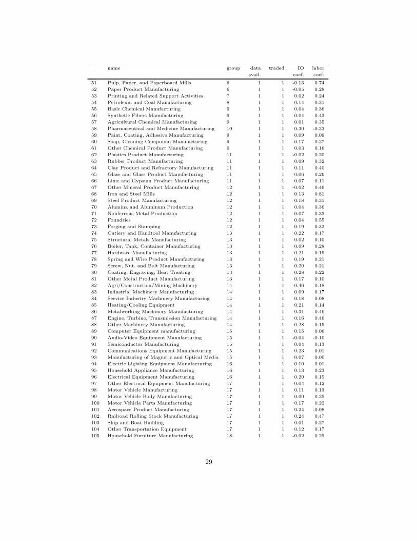
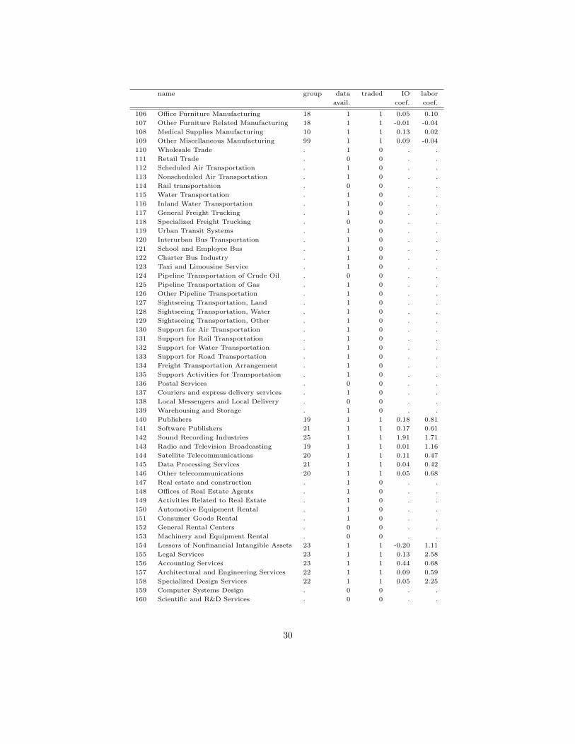
B Industry list with IO and labor coefficients (EG)

name group data traded IO labor

avail. coef. coef.

1 Crop production . 0 0 . .

2 Animal production . 0 0 . .

3 Aviculture . 0 0 . .

4 Mixed agriculture . 0 0 . .

5 Silviculture . 0 0 . .

6 Forestry . 0 0 . .

7 Logging . 0 0 . .

8 Fishing . 0 0 . .

9 Hunting and Trapping . 0 0 . .

10 Support Activities for Crop Production . 0 0 . .

11 Support Activities for Animal Production . 0 0 . .

12 Support Activities for Forestry . 0 0 . .

13 Oil and Gas Extraction 1 1 1 0.27 -0.26

14 Coal Mining 1 1 1 0.06 0.97

15 Metal Ore Mining 1 1 1 -0.02 0.82

16 Nonmetallic Mineral Mining and Quarrying 1 1 1 -0.04 0.47

17 Support Activities for Mining 1 1 1 0.36 0.95

18 Utilities . 1 0 . .

19 Utility System Construction . 1 0 . .

20 Land Subdivision . 1 0 . .

21 Highway, Street, and Bridge Construction . 1 0 . .

22 Heavy and Civil Engineering Construction . 1 0 . .

23 Building Exterior Contractors . 1 0 . .

24 Building Equipment Contractors . 1 0 . .

25 Building Finishing Contractors . 1 0 . .

26 Other Specialty Trade Contractors . 1 0 . .

27 Animal Food Manufacturing 2 1 1 0.01 0.24

28 Grain and Oilseed Milling 2 1 1 -0.09 0.35

29 Sugar Product Manufacturing 2 1 1 0.01 0.19

30 Fruit and Vegetable Preserving 2 1 1 -0.00 0.23

31 Dairy Product Manufacturing 2 1 1 -0.16 0.16

32 Animal slaughtering and processing 2 1 1 0.02 0.54

33 Seafood Preparation and Packaging 2 1 1 0.14 -0.06

34 Bakeries and Tortilla Manufacturing 2 1 1 0.08 -0.10

35 Other Food Manufacturing 2 1 1 0.01 0.07

36 Beverage Manufacturing 2 1 1 0.02 0.13

37 Tobacco Manufacturing 3 1 1 0.26 0.35

38 Fiber, Yarn, and Thread Mills 4 1 1 -0.11 2.10

39 Textile and Fabric Mills 4 1 1 0.28 -0.18

40 Textile furnishings mills 4 1 1 0.16 0.21

41 Other Textile Product Mills 4 1 1 -0.01 0.12

42 Apparel Knitting Mills 4 1 1 -0.04 0.69

43 Cut and Sew Apparel Manufacturing 4 1 1 0.31 0.21

44 Other Apparel Manufacturing 4 1 1 0.37 -0.09

45 Leather and Hide Tanning 4 1 1 0.10 0.38

46 Footwear Manufacturing 4 1 1 0.13 0.31

47 Other Leather Manufacturing 4 1 1 0.00 0.11

48 Sawmills and Wood Preservation 5 1 1 0.05 0.64

49 Wood product Manufacturing 5 1 1 0.11 0.31

50 Other Wood Product Manufacturing 5 1 1 0.10 0.22

28

name group data traded IO labor

avail. coef. coef.

51 Pulp, Paper, and Paperboard Mills 6 1 1 -0.13 0.74

52 Paper Product Manufacturing 6 1 1 -0.05 0.28

53 Printing and Related Support Activities 7 1 1 0.02 0.24

54 Petroleum and Coal Manufacturing 8 1 1 0.14 0.31

55 Basic Chemical Manufacturing 9 1 1 0.04 0.36

56 Synthetic Fibers Manufacturing 9 1 1 0.04 0.43

57 Agricultural Chemical Manufacturing 9 1 1 0.01 0.35

58 Pharmaceutical and Medicine Manufacturing 10 1 1 0.30 -0.33

59 Paint, Coating, Adhesive Manufacturing 9 1 1 0.09 0.09

60 Soap, Cleaning Compound Manufacturing 9 1 1 0.17 -0.27

61 Other Chemical Product Manufacturing 9 1 1 0.03 0.16

62 Plastics Product Manufacturing 11 1 1 -0.02 0.20

63 Rubber Product Manufacturing 11 1 1 0.09 0.32

64 Clay Product and Refractory Manufacturing 11 1 1 0.11 0.40

65 Glass and Glass Product Manufacturing 11 1 1 0.06 0.26

66 Lime and Gypsum Product Manufacturing 11 1 1 0.07 0.11

67 Other Mineral Product Manufacturing 12 1 1 -0.02 0.46

68 Iron and Steel Mills 12 1 1 0.13 0.81

69 Steel Product Manufacturing 12 1 1 0.18 0.35

70 Alumina and Aluminum Production 12 1 1 0.04 0.36

71 Nonferrous Metal Production 12 1 1 0.07 0.33

72 Foundries 12 1 1 0.04 0.55

73 Forging and Stamping 12 1 1 0.19 0.32

74 Cutlery and Handtool Manufacturing 13 1 1 0.22 0.17

75 Structural Metals Manufacturing 13 1 1 0.02 0.10

76 Boiler, Tank, Container Manufacturing 13 1 1 0.09 0.28

77 Hardware Manufacturing 13 1 1 0.21 0.19

78 Spring and Wire Product Manufacturing 13 1 1 0.19 0.21

79 Screw, Nut, and Bolt Manufacturing 13 1 1 0.20 0.21

80 Coating, Engraving, Heat Treating 13 1 1 0.28 0.22

81 Other Metal Product Manufacturing 13 1 1 0.17 0.10

82 Agri/Construction/Mining Machinery 14 1 1 0.46 0.18

83 Industrial Machinery Manufacturing 14 1 1 0.09 0.17

84 Service Industry Machinery Manufacturing 14 1 1 0.18 0.08

85 Heating/Cooling Equipment 14 1 1 0.21 0.14

86 Metalworking Machinery Manufacturing 14 1 1 0.31 0.46

87 Engine, Turbine, Transmission Manufacturing 14 1 1 0.16 0.46

88 Other Machinery Manufacturing 14 1 1 0.28 0.15

89 Computer Equipment manufacturing 15 1 1 0.15 0.06

90 Audio-Video Equipment Manufacturing 15 1 1 -0.04 -0.10

91 Semiconductor Manufacturing 15 1 1 0.04 0.13

92 Communications Equipment Manufacturing 15 1 1 0.23 0.01

93 Manufacturing of Magnetic and Optical Media 15 1 1 0.07 0.00

94 Electric Lighting Equipment Manufacturing 16 1 1 0.10 0.01

95 Household Appliance Manufacturing 16 1 1 0.13 0.23

96 Electrical Equipment Manufacturing 16 1 1 0.20 0.15

97 Other Electrical Equipment Manufacturing 17 1 1 0.04 0.12

98 Motor Vehicle Manufacturing 17 1 1 0.11 0.13

99 Motor Vehicle Body Manufacturing 17 1 1 0.00 0.25

100 Motor Vehicle Parts Manufacturing 17 1 1 0.17 0.22

101 Aerospace Product Manufacturing 17 1 1 0.24 -0.08

102 Railroad Rolling Stock Manufacturing 17 1 1 0.24 0.47

103 Ship and Boat Building 17 1 1 0.01 0.27

104 Other Transportation Equipment 17 1 1 0.12 0.17

105 Household Furniture Manufacturing 18 1 1 -0.02 0.29

29

name group data traded IO labor

avail. coef. coef.

106 Office Furniture Manufacturing 18 1 1 0.05 0.10

107 Other Furniture Related Manufacturing 18 1 1 -0.01 -0.04

108 Medical Supplies Manufacturing 10 1 1 0.13 0.02

109 Other Miscellaneous Manufacturing 99 1 1 0.09 -0.04

110 Wholesale Trade . 1 0 . .

111 Retail Trade . 0 0 . .

112 Scheduled Air Transportation . 1 0 . .

113 Nonscheduled Air Transportation . 1 0 . .

114 Rail transportation . 0 0 . .

115 Water Transportation . 1 0 . .

116 Inland Water Transportation . 1 0 . .

117 General Freight Trucking . 1 0 . .

118 Specialized Freight Trucking . 0 0 . .

119 Urban Transit Systems . 1 0 . .

120 Interurban Bus Transportation . 1 0 . .

121 School and Employee Bus . 1 0 . .

122 Charter Bus Industry . 1 0 . .

123 Taxi and Limousine Service . 1 0 . .

124 Pipeline Transportation of Crude Oil . 0 0 . .

125 Pipeline Transportation of Gas . 1 0 . .

126 Other Pipeline Transportation . 1 0 . .

127 Sightseeing Transportation, Land . 1 0 . .

128 Sightseeing Transportation, Water . 1 0 . .

129 Sightseeing Transportation, Other . 1 0 . .

130 Support for Air Transportation . 1 0 . .

131 Support for Rail Transportation . 1 0 . .

132 Support for Water Transportation . 1 0 . .

133 Support for Road Transportation . 1 0 . .

134 Freight Transportation Arrangement . 1 0 . .

135 Support Activities for Transportation . 1 0 . .

136 Postal Services . 0 0 . .

137 Couriers and express delivery services . 1 0 . .

138 Local Messengers and Local Delivery . 0 0 . .

139 Warehousing and Storage . 1 0 . .

140 Publishers 19 1 1 0.18 0.81

141 Software Publishers 21 1 1 0.17 0.61

142 Sound Recording Industries 25 1 1 1.91 1.71

143 Radio and Television Broadcasting 19 1 1 0.01 1.16

144 Satellite Telecommunications 20 1 1 0.11 0.47

145 Data Processing Services 21 1 1 0.04 0.42

146 Other telecommunications 20 1 1 0.05 0.68

147 Real estate and construction . 1 0 . .

148 Offices of Real Estate Agents . 1 0 . .

149 Activities Related to Real Estate . 1 0 . .

150 Automotive Equipment Rental . 1 0 . .

151 Consumer Goods Rental . 1 0 . .

152 General Rental Centers . 0 0 . .

153 Machinery and Equipment Rental . 0 0 . .

154 Lessors of Nonfinancial Intangible Assets 23 1 1 -0.20 1.11

155 Legal Services 23 1 1 0.13 2.58

156 Accounting Services 23 1 1 0.44 0.68

157 Architectural and Engineering Services 22 1 1 0.09 0.59

158 Specialized Design Services 22 1 1 0.05 2.25

159 Computer Systems Design . 0 0 . .

160 Scientific and R&D Services . 0 0 . .

30

name group data traded IO labor

avail. coef. coef.

161 Advertising and Related Services . 0 0 . .

162 Professional and Scientific Services . 0 0 . .

163 Management of Companies and Enterprises 23 1 1 0.07 0.46

164 Office Administrative Services 23 1 1 -0.04 0.54

165 Facilities Support Services 23 1 1 0.07 0.71

166 Management Consulting Services 23 1 1 0.12 0.13

167 Business Support Services 24 1 1 0.04 0.21

168 Travel Arrangement Services . 1 0 . .

169 Investigation and security services . 1 0 . .

170 Services to Buildings and Dwellings . 0 0 . .

171 Other Support Services . 0 0 . .

172 Waste Treatment and Disposal . 1 0 . .

173 Elementary and Secondary Schools . 1 0 . .

174 Junior Colleges 24 1 1 0.32 0.57

175 Colleges, Universities, Professional Schools 24 1 1 0.07 0.38

176 Business Schools and Computer Training 24 1 1 0.27 0.39

177 Technical and Trade Schools 24 1 1 0.13 0.10

178 Other Schools and Instruction . 1 0 . .

179 Educational Support Services . 1 0 . .

180 Offices of Physicians . 1 0 . .

181 Offices of Dentists . 1 0 . .

182 Offices of Other Health Practitioners . 0 0 . .

183 Medical and Diagnostic Laboratories . 0 0 . .

184 Home Health Care Services . 0 0 . .

185 Other Ambulatory Health Care Services . 1 0 . .

186 General Medical and Surgical Hospitals . 1 0 . .

187 Psychiatric and Substance Abuse Hospitals . 1 0 . .

188 Specialty Hospitals . 1 0 . .

189 Nursing Care Facilities . 1 0 . .

190 Mental Health and Substance Abuse Facilities . 1 0 . .

191 Individual and Family Services . 1 0 . .

192 Community Food and Housing . 1 0 . .

193 Vocational Rehabilitation Services . 1 0 . .

194 Child Day Care Services . 1 0 . .

195 Performing Arts Companies 25 1 1 -0.01 3.41

196 Spectator Sports 25 1 1 0.03 0.17

197 Promoters of Performing Arts 25 1 1 0.23 0.42

198 Agents and Managers 25 1 1 0.85 2.96

199 Independent Artists 25 1 1 0.26 2.19

200 Museums and Historical Sites 25 1 1 0.18 0.44

201 Amusement Parks and Recreation Industry 26 1 1 0.16 0.15

202 Traveler Accommodation 26 1 1 -0.00 0.13

203 RV Parks and Recreational Camps 26 1 1 -0.24 -0.17

204 Residential Care Facilities . 1 0 . .

205 Restaurants . 1 0 . .

206 Special Food Services . 1 0 . .

207 Drinking Places (Alcoholic Beverages) . 0 0 . .

208 Automotive Repair and Maintenance . 1 0 . .

209 Machinery Repair and Maintenance 27 1 1 0.05 0.31

210 Household Goods Repair and Maintenance . 1 0 . .

211 Other Personal Services . 1 0 . .

212 Associations and Organizations . 1 0 . .

213 Household services . 0 0 . .

214 Other Public Services . 1 0 . .

215 Finance and Insurance 23 1 1 0.07 0.53

31

Table B.1: Average point-estimates by industry group.

group name IO laborcoef. coef.

1 Extraction 0.13 0.592 Food Manufacturing 0.00 0.183 Tobacco Manufacturing 0.26 0.354 Textile Manufacturing 0.12 0.395 Wood products 0.09 0.396 Paper products -0.09 0.517 Printing 0.02 0.248 Petroleum and Coal Manufacturing 0.14 0.319 Chemical Manufacturing 0.06 0.1910 Pharmaceutical and medical supply 0.21 -0.1511 Materials 0.06 0.2612 Mineral products manufacturing 0.09 0.4513 Hardware Manufacturing 0.17 0.1814 Machinery 0.24 0.2315 Electronics 0.09 0.0216 Electrical equipment manufacuting 0.14 0.1317 Transportation Equipment 0.11 0.1918 Forniture 0.01 0.1219 Media 0.09 0.9920 Telecommunication 0.08 0.5721 IT services 0.10 0.5122 Architecture and Engineering 0.07 1.4223 Professional KIBS 0.08 0.8424 Educational 0.16 0.3325 Art and culture 0.49 1.6126 Recreation -0.03 0.0427 Machinery repair 0.05 0.3199 Other 0.09 -0.04

C Analysis using Location Correlation

Table C.1 shows the top 10 industry pairs for the co-agglomeration index based on location correlation,

see equation (2).

Table C.2 replicates table 7 of the main text for the LC-based coagglomeration measure. Here value

chain links are more important drivers of coagglomeration than labor pooling.

Figure C.1 replicates figure 2 of the main text for the LC-based coagglomeration measure. As in the

main text for the EG measure, the effect sizes are quite heterogeneous. Both types of inter-industry

similarities exert a greater influence on coagglomeration in services than in manufacturing industries.

However, the variation is particularly pronounced when it comes to the effect of labor similarities.

32

Table C.1: Top-10 industry pairs by coagglomeration (locational correlation index)

Top-10 co-location (LC index)

industry i industry j valueIndependent Artists Cut and Sew Apparel Manufacturing 0.9915Legal Services Finance and Insurance 0.9900Independent Artists Accounting Services 0.9877Specialized Design Services Legal Services 0.9873Sound Recording Industries Agents and Managers 0.9861Publishers Performing Arts Companies 0.9854Radio and Television Broadcasting Legal Services 0.9840Publishers Legal Services 0.9837Cut and Sew Apparel Manufacturing Agents and Managers 0.9834Cut and Sew Apparel Manufacturing Accounting Services 0.9812

Idem table 1 but here we show the top-10 industry pairs using the LC-based coagglomeration metric (see equation (2))using city-industry employment data for the US (County Business Patterns, 2003).

Table C.2: OLS and IV univariate regressions on extended sample

(1) (2) (3) (4) (5) (6)OLS OLS OLS IV IV IVstate city county state city county

LC index

Input-output 0.132 0.119 0.122 0.162 0.148 0.139(0.015) (0.015) (0.015) (0.027) (0.028) (0.027)

Observations 7140 7140 7140 7140 7140 7140R2 0.024 0.021 0.026 0.023 0.020 0.026

Labor 0.120 0.033 0.044 0.061 -0.025 0.005(0.008) (0.008) (0.008) (0.017) (0.016) (0.015)

Observations 7140 7140 7140 7140 7140 7140R2 0.024 0.002 0.004 0.018 . 0.001

Robust standard errors in parentheses. Robust standard errors in parentheses.

Idem table 6 but in this case we use the LC correlation index in lieu of the EG index. These regressions also show that,in this extended sample, value chain and labor market links are even more important drivers of coagglomeration thanin the manufacturing only sample.

33

Figure C.1: Coagglomeration effects (LC-index), manufacturing versus services

Extraction

FoodTobacco

Textile

Wood products

Paper products Printing

Petroleum & Coal

Chemical

Pharma & medical

Materials

Mineral products

Hardware Machinery

ElectronicsElectrical eqpt

Transportation eqpt

Furniture

Media

Telecommunication

IT services

Architecture & Engineering

KIBS

Education

Art & culture

RecreationMachinery repair

-.20

.2.4

.6.8

β L

-.1 0 .1 .2 .3

β IO

Labor pooling effects (vertical axis) and value chain effects (horizontal axis). The panel on the left reports re-

sults of an OLS regression. Estimates for the coagglomeration patterns of services are plotted in red, those for

manufacturing industries in blue. The crosshairs represent 95% confidence intervals based on robust standard errors.

D Correction to CBP censoring

In CBP, when the information in a cell (by geography and by industry) reveals information about a

firm, the data in the cell is withheld by the Census to avoid disclosure. However in this case CBP

offers information about the employment size class. To attribute a single employment value to the

employment range of the class, we follow Holmes and Stevens (2004), where the authors provide the

following estimate (obtained using national data and a model) of the mean employment for CBP class

in the year 2000.

34

Table D.1: Mean employment by size class in 2000 CBP, as in Holmes and Stevens (2004)

Employment Averagerange employment

1-4 1.75-9 6.610-19 13.520-49 30.250-99 68.8100-249 150.1250-499 340.7500-999 681.31000-1499 1208.81500-2499 1892.92500-4999 3374.75000 or more 9592.0

The CBP classes have changed slightly since Holmes and Stevens (2004). We adapt their estimates

to the new classes as follows: categories C, E, F and H use directly their estimate. Categories A, B

and G use weighted average from the sub-classes in Holmes and Stevens (2004). Categories I, J, K

and L use the average ratio between the estimated employment of classes A to G and the mid-point

of the employment classes A to G (0.7974). This ratio is then multiplied by the midpoint of I, J, K

and L to obtain an estimate. Categories M lacks an upper bound to compute the mid-point. 125000

is obtained multiplying 100000 by the average of the ratio between minimum and estimated mean of

classes I through L. The resulting scheme is used in this paper

Table D.2: Mean employment by size class in 2003 and 2008 CBP, as used in this paper

Class Employment Averagerange employment

A 0-19 5B 20-99 40C 100-249 150E 250-499 341F 500-999 681G 1,000-2,499 1488H 2,500-4,999 3375I 5,000-9,999 5980J 10,000-24,999 13955K 25,000-49,999 29904L 50,000-99,999 59804M 100,000 or More 125000

35