Paper SD-84 Expanding the Use of Weight of Evidence and ... · Scorecard Development Alec Zhixiao Lin, PayPal Credit, Timonium, MD Tung-Ying Hsieh, Dept. of Mathematics & Statistics,

SESUG 2014

1

Paper SD-84

Expanding the Use of Weight of Evidence and Information Value to Continuous Dependent Variables for Variable Reduction and

Scorecard Development Alec Zhixiao Lin, PayPal Credit, Timonium, MD

Tung-Ying Hsieh, Dept. of Mathematics & Statistics, Univ of Maryland, Baltimore, MD

ABSTRACT

Weight of Evidence (WOE) and Information Value (IV) have become important tools for analyzing and modeling binary outcomes such as default in payment, response to a marketing campaign, etc. By suggesting a set of alternative formulae, this paper attempts to expand their use to continuous outcomes such as sales volume, claim

amount, etc. A SAS®

macro program is provided that will efficiently evaluate the predictive power of continuous,

ordinal and categorical variables together and yield useful suggestions for variable reduction/selection and for segmentation. Modelers can use the insights conveyed by SAS outputs for subsequent linear regression, logistic regression or scorecard development.

INTRODUCTION

Based on the information theory conceived in later 1940s and initially developed for scorecard development, Weight of Evidence (WOE) and Information Value (IV) have been gaining increasing attention in recent years for such uses as segmentation and variable reduction. As the calculation of WOE and IV requires the contrast between occurrence and non-occurrence (usually denoted by 1 and 0), their use has largely been restricted to the analysis of and prediction for binary outcomes such as default in payment, response to a marketing campaign, etc.

This paper attempts to expand the use of WOE and IV to continuous dependent variables such as sales, revenue and loss amount, etc. We will first propose a set of alternative formulae of WOE and IV for binary dependent variables and examine their similarities to and differences from the original formulae. We then go on to explore why and how the alternative formulae can be adapted to the setting of continuous dependent variables. Moreover, the paper provides SAS macro program that can be used to assess the predictive power of continuous, ordinal and categorical independent variables together. Apart from greatly expediting the process of variable reduction/selection, the multiple SAS outputs can provide useful suggestions for segmentation or scorecard development as well as for other purposes such as imputation for missing values, flooring and ceiling variables, creating class variables, etc.

IV AND WOE FOR BINARY DEPENDENT VARIABLES

Weight of Evidence (WOE) recodes the values of a variable into discrete categories and assigns to each category a unique WOE value in the purpose of producing the largest differences between the recoded. An important assumption here is that the dependent variable should be binary to denote occurrence and non-occurrence of an event. In the example of risk analysis when an account is either current (good) or delinquent (bad), WOE for any segment of customers is calculated as follows with Table 1 illustrating how it looks:

WOE = [ln (%𝐵𝑎𝑑𝑖%𝐺𝑜𝑜𝑑𝑖

)] × 100

Table 1. WOE for A Risk Score

To better understand WOE, we would like to stress the following:

SESUG 2014

2

%Bad is not equivalent %Bad Rate. % Bad is the percentage of bad accounts in a score band over all bad counts. Same understanding applies to %Good in the example.

It does not matter whether %Good or %Bad should be chosen as the numerator. If the two measures exchange their positions in the division, the sign of WOE for each score band will reverse while the magnitude will remain unchanged. There is no impact on the subsequent calculation for IV.

Multiplication by 100 is optional. Based on WOE, IV assesses the overall predictive power of the variable. Therefore, it can be used for evaluating the predictive power among competing variables. The following is how Information Value is calculated:

𝐼𝑉 =∑ ((%𝐵𝑎𝑑𝑖 −%𝐺𝑜𝑜𝑑𝑖) × ln(%𝐵𝑎𝑑𝑖%𝐺𝑜𝑜𝑑𝑖

))

𝑛

𝑖=1

For inferences, we would like to point out the following:

Even though higher-IV variables are thought to be more predictive, it does not mean they are ready to enter a regression model directly. The magnitude of IV is not dependent upon the monotonicity of the variable in relation to the target outcome. If two score bands in Table 1 exchange their %Bad Rate, this will result in no change in IV, but a variable as such becomes less useful for regression;

If WOE of a numeric variable changes from highest to lowest (as in Table 1) or vice versa, it usually suggests a good monotonicity and the variable becomes a good candidate for a regression model. Figure 1 and Figure 2 illustrate this point with two variables, one with a good monotonicity and the other without;

If a categorical variable shows a high IV, it can provide suggestion for segmentation.

What if the dependent variable is continuous such as revenue, sales volume and loss amount? If an outcome is no longer binary, the above formulae for WOE and IV fail to apply. In the example of sales volume, we can still get %Sales (percentage of sales in a bin over total sales volume), but %NoSales is utterly unconceivable.

WOE AND IV: ALTERMATIVE FORMULAE

Let’s examine an alternative set of formulae for the same risk analysis as in the previous section:

WOE = [ln (%𝐵𝑎𝑑𝑖

%𝑅𝑒𝑐𝑜𝑟𝑑𝑠𝑖)] × 100

𝐼𝑉 =∑ ((%𝐵𝑎𝑑𝑖 −%𝑅𝑒𝑐𝑜𝑟𝑑𝑠𝑖) × ln(%𝐵𝑎𝑑𝑖

%𝑅𝑒𝑐𝑜𝑟𝑑𝑠𝑖))

𝑛

𝑖=1

Instead of contrasting %Good with %Bad, the formulae above replace %Good with %Records, which is the percentage of accounts in a score band over all accounts, as illustrated by Table 2.

Score Band # Records %Records # Bad # Good % Bad % Good

original

WOE

alterntive

WOE % Bad Rate

1-50 20,534 6.5% 1,581 18,953 16.1% 6.2% 95.30 90.46 7.7%

51-100 23,000 7.3% 1,382 21,618 14.1% 7.1% 68.69 65.66 6.0%

101-150 18,567 5.9% 888 17,679 9.0% 5.8% 44.58 42.84 4.8%

151-200 37,842 12.0% 1,362 36,480 13.8% 11.9% 14.91 14.41 3.6%

201-250 45,687 14.5% 1,325 44,362 13.5% 14.5% -7.40 -7.18 2.9%

251-300 55,698 17.6% 1,392 54,306 14.2% 17.8% -22.69 -22.06 2.5%

301-350 45,768 14.5% 961 44,807 9.8% 14.7% -40.52 -39.48 2.1%

351-400 33,458 10.6% 569 32,889 5.8% 10.8% -62.01 -60.56 1.7%

401-450 20,093 6.4% 241 19,852 2.5% 6.5% -97.43 -95.47 1.2%

451-500 15,008 4.8% 135 14,873 1.4% 4.9% -126.51 -124.25 0.9%

Total 315,655 100.0% 9,836 305,819 100.0% 100.0%

Table 2. Alternative Formula for WOE How do the resultant WOE and IV look like compared to those generated by the original formulae? Figure 1 and Figure 2 shows two examples of WOEs, one with good monotonicity and the other without:

SESUG 2014

3

Figure 1. WOE and Good Monotonicity Figure 2. WOE and Bad Monotonicity

For a score band with %Good > %Bad, the WOE by the alternative formula is lower. Otherwise, the WOE by the alternative formula is higher. We use a sample of 115 variables to compare the IVs generated by the two versions of formulae and examine how they trend together. The average rate of occurrence here, i.e., %Bad Rate, is 3%.

0

0.05

0.1

0.15

0.2

0.25

0.3

x1 x4 x7 x10

x13

x16

x19

x22

x25

x28

x31

x34

x37

x40

x43

x46

x49

x52

x55

x58

x61

x64

x67

x70

x73

x76

x79

x82

x85

x88

x91

x94

x97

x100

x103

x106

x109

x112

x115

Info

rmat

ion

Valu

e

Variable

original IV

alternative IV

Figure 3. IV Comparison Based on A Rare Event

In Figure 3 the two formulae yield exactly the same rank order in terms of IV for all variables, with alternative IV looking slightly weaker across the board. An intuitive explanation for this minor discrepancy in IV is: as %Records contains both good and bad accounts, the contrast between %Bad and %Records is less strong than the contrast between %Bad and %Good. In the above example, as average %Bad Rate is around 3%, %Records and %Good in each bin look quite close, hence very close IVs across all variables. In such cases, we consider following rules of thumb suggested by Siddiqi for evaluating IV still applies to the binary dependent variable for the alternative IV:

< 0.02: unpredictive 0.02 to 0.1: weak 0.1 to 0.3: medium 0.3 to 0.5: strong > 0.5: suspicious

However, if the target variable exhibits very high rate of occurrence, such as influenza infection rate and recidivism rate (all could be as high as 50%), the difference between %Good and %Records is much bigger, so the difference in IV produced by the two formulae is also likely to be bigger. Moreover, the values of WOE and the associated IV will be smaller, and the above rule of thumb for evaluating the predictive power of independent variables will no longer apply. The following chart is an example of payment by 30-day-only delinquent credit card accounts. The average likelihood of payment by these customers is around 75% as most customers just forget to make the payment in time rather than encountering some financial difficulty.

SESUG 2014

4

0

0.005

0.01

0.015

0.02

0.025

0.03

0.035

0.04

0

0.05

0.1

0.15

0.2

0.25

0.3

0.35

0.4

0.45

0.5

x1 x5 x9 x13

x17

x21

x25

x29

x33

x37

x41

x45

x49

x53

x57

x61

x65

x69

x73

x77

x81

x85

x89

x93

x97

x101

x105

x109

x113

x117

alter

nativ

e IV

Origi

nal IV

Variable

original IV

alternative IV

Figure 4. IV Comparison Based on A Very Common Event

Despite forsaking the use of the rule of thumb for IV evaluation, the relative ranking of IVs across all variables look quite similar or close in Figure 4. In modeling and segmentation, the relative ranking of predictive power is more relevant in variable evaluation. As the alternative formulae no longer require a direct contrast between occurrence and non-occurrence, they can be potentially useful for analyzing and modeling continuous dependent variables.

WOE AND IV FOR CONTINUOUS DEPENDENT VARIABLES

Let’s use an example of sales volume to illustrate how to use the alternative formulae to calculate WOE and IV:

WOE = [ln (%𝑆𝑎𝑙𝑒𝑠𝑖

%𝑅𝑒𝑐𝑜𝑟𝑑𝑠𝑖)] × 100

𝐼𝑉 =∑ ((%𝑆𝑎𝑙𝑒𝑠𝑖 −%𝑅𝑒𝑐𝑜𝑟𝑑𝑠𝑖) × ln(%𝑆𝑎𝑙𝑒𝑠𝑖

%𝑅𝑒𝑐𝑜𝑟𝑑𝑠𝑖))

𝑛

𝑖=1

The following table compares the WOEs and IVs of three variables in predicting sales volume.

Variable A # Records %Records Sales Volume % Sales WOE

1 1,000 10% 80 1.8% -170.47

2 1,000 10% 160 3.6% -101.16

3 1,000 10% 240 5.5% -60.61

4 1,000 10% 320 7.3% -31.85

5 1,000 10% 400 9.1% -9.53

6 1,000 10% 480 10.9% 8.70

7 1,000 10% 560 12.7% 24.12

8 1,000 10% 640 14.5% 37.47

9 1,000 10% 720 16.4% 49.25

10 1,000 10% 800 18.2% 59.78

Total 10,000 100% 4400 100.0%

IV for Variable A: 0.346

Variable B # Records %Records # Sales % Sales WOE

1 1,000 10% 100 2.3% -148.16

2 1,000 10% 540 12.3% 20.48

3 1,000 10% 400 9.1% -9.53

4 1,000 10% 340 7.7% -25.78

5 1,000 10% 448 10.2% 1.80

6 1,000 10% 412 9.4% -6.58

7 1,000 10% 660 15.0% 40.55

8 1,000 10% 523 11.9% 17.28

9 1,000 10% 321 7.3% -31.53

10 1,000 10% 656 14.9% 39.94

Total 10,000 100% 4400 100.0%

IV for Variable B: 0.178

Variable C # Records %Records # Sales % Sales WOE

1 1,400 14% 100 2.3% -181.81

2 200 2% 155 3.5% 56.61

3 400 4% 290 6.6% 49.94

4 800 8% 320 7.3% -9.53

5 800 8% 448 10.2% 24.12

6 800 8% 437 9.9% 21.63

7 1,300 13% 600 13.6% 4.78

8 1,400 14% 590 13.4% -4.31

9 1,400 14% 700 15.9% 12.78

10 1,500 15% 760 17.3% 14.11

Total 10,000 100% 4400 100.0%

IV for Variable C: 0.251

Even though the performance by

the target variable looks

reasonably good, the

distribution of Variable C is less

good. Too many sales

concentrates on top tiers, which

suggests low differentiating

power and hence lower IV.

A perfectly even distribution

with a good performance a the

target variable. Variable A is

expected to be a good candidate

for linear regression.

Comment

Comment

A perfectly even distribution

with a somewhat weaker

performance by the target

variable. Variable B cannot

compete with Variable A, and its

IV is expected to be lower.

Comment

Table 3. WOE for A Continuous Outcome

SESUG 2014

5

We have noticed the following differences when applying the alternative formulae to binary dependent variables and to continuous dependent variables:

For a binary outcome, each record weighs and contributes equally to WOE and IV. But in the case of a continuous outcome, higher-volume records contribute more and hence exert more impact. In the example of sales volume, a record of 1000 sales weighs more in %sales than another record of 200 purchases. Outliers in a continuous variable could exert an out-of-proportion influence. In such cases, outliers should be trimmed. A log transformation or other methods can also be employed to make the disparity less heightened.

Outliers in an independent variable are of a much less concern in evaluation by WOE and IV since they are effectively suppressed by binning. They still need to be trimmed in a subsequent regression.

THE SAS PROGRAM

Let’s strike a note of comfort first: the SAS programs enclosed in the appendices are long and look intimidating, but most users only need to make several changes to lines in Part in order to use the program. We suggest doing the following before running it:

Save the two programs from APPENDIX 2-a and APPENDIX 2-b into a designated folder. These two programs will be invoked by the %INCLUDE statement in the SAS macro.

Run PROC CONTENTS to separate categorical and numerical variables. All categorical variables should be expressed as characters. Convert ordinal variables to character and group them with categorical variables.

Run PROC MEANS to screen out variables with no coverage or with a uniform value. You can also consider deleting variables with very low coverage. This will reduce the file size and processing time.

Apply business knowledge to bin categorical values beforehand if needed. The program will bin numeric values for evaluation, but does not do so to categorical or ordinal values.

Ensure the list of independent variables contains no duplicates. Duplicates will produce erroneous results. The SAS program is equally applicable to both binary and continuous outcomes. If the target variable is continuous, alternative WOE and IV will be computed. If the target variable is binary, the program reverts to the calculation of original WOE and IV. The following is the beginning part of program: ** Part I – SPECIFY THE DATA SET AND VARIABLES;

libname your_lib "folder where your SAS data is stored";

%let libdata=your_lib; /* libname defined in the previous line */

%let inset=your_sas_dataset; /* your SAS data set */

%let vartxt=xch1 xch2 …; /* all categorical and ordinal variables.

Variables should be in character format only. Use vartxt= if none */

%let varnum=xnum1 xnum2 …; /* all numeric variables. Use varnum= if none */

%let target=y; /* target variable (y) */

%let ytype=continue; /* continue=continuous outcome, binary=binary outcome */

%let outname=sales volume; /* label of target y for summary tables and graphs */

%let targetvl=15.2; /* change to percent8.4 or others for binary outcomes */

%let libout=the folder where SAS outputs are sent to; /* e.g., c:\folder */

**Part II – CHANGE THE FOLLOWING AS YOU SEE FIT;

%let tiermax=10; /* maximum number of bins for continuous variables */

%let ivthresh=0; /* threshold of IV for graphing.

If you would like to see graphs of all variables, set this to 0.

For a continuous outcome, always set this to 0 */

%let capy=98; /* outlier cap for continuous outcomes.

This macro value has no impact on binary outcomes */

%let formtall=20.6; /* a format that accommodates all numeric variables */

%let tempmiss=-1000000000000; /* flag of missing values for numeric variables */

%let charmiss=_MISSING_; /* flag of missing values for categorical variables */

%let outgraph=gh; /* name pdf graph for predictors */

%let ivout=iv; /* name output file for IV */

%let woeout=woe; /* name of output file for WOE */

**Part III – DO NOT CHANGE ANYTHING FROM HERE ON;

%macro kicknum;

%let numcount = %sysfunc(countw(&varnum dummyfill));

%if &numcount > 1 %then %do;

%include "SAS program from Appendix 2-a";

%end;

SESUG 2014

6

%mend;

%kicknum;

%macro kickchar;

%let charcount = %sysfunc(countw(&vartxt dummyfill));

%if &charcount > 1 %then %do;

%include "SAS program from Appendix 2-b";

%end;

%mend;

%kickchar;

(Subsequent part of the program can be found in the appendices.)

SAS OUTPUTS

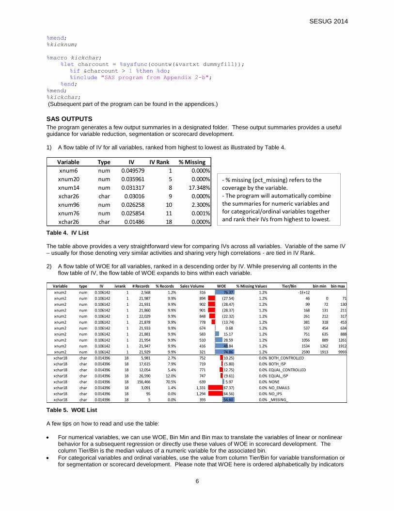
The program generates a few output summaries in a designated folder. These output summaries provides a useful guidance for variable reduction, segmentation or scorecard development. 1) A flow table of IV for all variables, ranked from highest to lowest as illustrated by Table 4.

Variable Type IV IV Rank % Missing

xnum6 num 0.049579 1 0.000%

xnum20 num 0.035961 5 0.000%

xnum14 num 0.031317 8 17.348%

xchar26 char 0.03016 9 0.000%

xnum96 num 0.026258 10 2.300%

xnum76 num 0.025854 11 0.001%

xchar26 char 0.01486 18 0.000%

Table 4. IV List

The table above provides a very straightforward view for comparing IVs across all variables. Variable of the same IV – usually for those denoting very similar activities and sharing very high correlations - are tied in IV Rank. 2) A flow table of WOE for all variables, ranked in a descending order by IV. While preserving all contents in the

flow table of IV, the flow table of WOE expands to bins within each variable.

Variable type IV ivrank # Records % Records Sales Volume WOE % Missing Values Tier/Bin bin min bin max

xnum2 num 0.106142 1 2,568 1.2% 316 76.37 1.2% -1E+12

xnum2 num 0.106142 1 21,987 9.9% 894 (27.54) 1.2% 46 0 71

xnum2 num 0.106142 1 21,931 9.9% 902 (28.47) 1.2% 99 72 130

xnum2 num 0.106142 1 21,860 9.9% 901 (28.37) 1.2% 168 131 211

xnum2 num 0.106142 1 22,029 9.9% 848 (22.32) 1.2% 261 212 317

xnum2 num 0.106142 1 21,878 9.9% 778 (13.74) 1.2% 381 318 453

xnum2 num 0.106142 1 21,933 9.9% 674 0.68 1.2% 537 454 634

xnum2 num 0.106142 1 21,881 9.9% 583 15.17 1.2% 751 635 888

xnum2 num 0.106142 1 21,954 9.9% 510 28.59 1.2% 1056 889 1261

xnum2 num 0.106142 1 21,947 9.9% 416 48.84 1.2% 1534 1262 1912

xnum2 num 0.106142 1 21,929 9.9% 321 74.86 1.2% 2590 1913 9993

xchar18 char 0.014396 18 5,981 2.7% 752 (10.25) 0.0% BOTH_CONTROLLED

xchar18 char 0.014396 18 17,615 7.9% 719 (5.80) 0.0% BOTH_ISP

xchar18 char 0.014396 18 12,054 5.4% 771 (12.75) 0.0% EQUAL_CONTROLLED

xchar18 char 0.014396 18 26,590 12.0% 747 (9.61) 0.0% EQUAL_ISP

xchar18 char 0.014396 18 156,466 70.5% 639 5.97 0.0% NONE

xchar18 char 0.014396 18 3,091 1.4% 1,331 (67.37) 0.0% NO_EMAILS

xchar18 char 0.014396 18 95 0.0% 1,294 (64.56) 0.0% NO_IPS

xchar18 char 0.014396 18 5 0.0% 393 54.60 0.0% _MISSING_

Table 5. WOE List

A few tips on how to read and use the table:

For numerical variables, we can use WOE, Bin Min and Bin max to translate the variables of linear or nonlinear behavior for a subsequent regression or directly use these values of WOE in scorecard development. The column Tier/Bin is the median values of a numeric variable for the associated bin.

For categorical variables and ordinal variables, use the value from column Tier/Bin for variable transformation or for segmentation or scorecard development. Please note that WOE here is ordered alphabetically by indicators

- % missing (pct_missing) refers to the coverage by the variable. - The program will automatically combine the summaries for numeric variables and for categorical/ordinal variables together and rank their IVs from highest to lowest.

SESUG 2014

7

shown in column Tier/Bin. Users will see how these indicators are re-ranked by performance outcome in the next section of SAS output.

3) A PDF collage of WOE for all variables above a specified threshold of IV, with three graphs for each variable.

Modelers will find these graphs to be useful for multiple purposes such as:

Providing good visual aids for variable distribution and a trend line in relation to the target outcome1.

Offering useful suggestions for imputing missing values.

Offering useful suggestions for how to group bins and to floor or cap a variable.

Even though categorical variables (including ordinal variable in our case) and numeric variables are assessed together, the output for these two types of variables are a bit different. Graphs in Figure 5 list outputs for a numeric variable:

Figure 5. Graphs for A Numeric Variable

Graphs in Figure 6 illustrate the use of graphic for categorical and ordinal variables. The third graph presents different contents than the one for numeric variables.

1 The SAS macro program provided by this paper does not provide optimal cuts between bins. Additional modules of SAS or other

computing tools are needed for generating optimal cuts.

The charts are ordered by IV from highest to lowest. ‘1’ means it is the most predictive power among all variables.

One can floor the risk_score as follows: if risk_score < 130 then risk_score=130.

risk_score=. can be imputed as risk_score=260 because of their similarity in behavior in terms of the target outcome.

Chart A: variable distribution and trend line

Chart C: variable distribution and trend line This chart shares some similarity with Chart A, with the following differences: - The distance between two points in X axis is the actual difference in value; - Missing values are not plotted.

Chart B: Graphic representation of WOE - In Chart A and Chart B, each value in x axis denotes the median value of the bin. - Equal distance between bins do not suggest equal difference between two medians. - If WOE ascends or descends in value from left to left, it usually suggests the variable can be a good candidate for a regression model.

SESUG 2014

8

Figure 6. Graphs for A Categorical Variable

For the subsequent linear/logistic regression or scorecard development, the author considers the following criteria for selecting potential predictors of similar Information Value to enter a final regression:

Magnitude of Information Value. Variables with higher Information Values are preferred;

Linearity. Variables exhibiting a strong linearity are preferred;

Coverage. Variables with fewer missing values are preferred;

Distribution. Variables with less uneven distributions are preferred;

Interpretation. Variables that make more sense in business are preferred.

TWO SPECIAL NOTES

Finally we would like to list two cases that call for some special attention, one with very very big data, and the other concerning two-stage modeling.

VERY VERY BIG DATA

Processing a large number of variables for a large data set usually runs into the problem of insufficient system memory. To partially overcome this problem, the SAS program in APPENDIX 1 automatically divides the data set into ten partitions for separate processing and then integrates the results into one output. If the issue of insufficient memory still persists, the following tips will help:

Chart A: variable distribution and trend line

‘5’ suggests that the variable has the 5th biggest IV.

Values in X axis are ordered alphabetically by the flags.

Chart B: Graphic representation of WOE

Chart C: variable distribution and trend line Flags for the categorical variables are ranked in a descending order by the target outcome. This helps modelers to group flags.

- The first two flags exhibits very similar behavior, they can be binned into one for modeling or segmentation. - One can also considering translating the categorical value into a numerical tier for modeling.

SESUG 2014

9

Run the SAS program on a reduced random sample. The order of IV might change slightly, but the general pattern still looks very similar;

Run PROC MEANS and/or PROC UNIVARIATE to screen out variables of extremely low coverages (e.g., < 1%) or with a uniform value.

If one works with a data set that contains an extremely large number of variables with numerous records (e.g., 10 million records with about 5000 variables), it is not uncommon that a high majority of variables have very low values and can be discarded in a wholesale manner. The program in Appendix 3 is developed for this purpose. Users can do the following: Step 1: Use the SAS program from Appendix 3 to run a preliminary screen. This SAS macro divides all variables into separate lists and processes each list separately. How many variables can be put into each individual list? It depends on the system capacity. Usually the larger the data set, the fewer variables you can put into a list. Step 2: Users can decide how many low-IV variables to discard and how many high-IV variables to retain. Please note that no PDF charts will be generated here in order to expedite the process. Step 3: For retained variables, run a closer examination by using the SAS program from Appendix 1 for a further reduction of variables. This time the SAS program will produce a complete suite of tables and graphs as illustrated before. Screening out low-IV variables can afford to be broad-brushed without losing value, so users are advised to run Step 1 and Step 2 on a reduced sample in order to speed up the process. In step 3 one will go back to the complete sample for evaluating a smaller list of retained variables.

SAMPLE WITH ZERO-INFLATED DEPENDENT VARIABLE

Suppose we need to build a model on claim amount on all insured accounts. A large number of customers do not make claims, so the continuous dependent variable contains a high portion of zero-value records. When encountering cases like this, we suggest separate treatments for segmentation and for regression. For segmentation, running a variable evaluation based on all accounts with claim amount as the target outcome will usually work fine, and SAS outputs can help analysts to choose the most “telling” variables for risk and to identify groups of more risky customers. However, the above results cannot be directly applied to a linear regression on claim amount. We suggest following the same logic as building a two-stage model and running a WOE and IV analysis in two separate steps: Step 1: Run an assessment by WOE and IV for the probability of occurrence (0 or 1) and build a model for probability estimation using logistic regression; Step 2: Run an assessment by WOE and IV for the claim amount based on accounts with claims. Afterwards one can build a linear model for claim amount only. Step 3: Multiply the probability estimate and amount estimate to get the expected claim amount.

CONCLUSION Even though Weight of Evidence and Information Value were developed for evaluating the binary outcomes, we can expand them to the analysis and modeling for continuous dependent variables. We hope the SAS program provided in the paper will greatly expedite the process of variable reduction/selection and provide meaningful business insights for important model attributes.

ACKNOWLEDGEMENTS I would like to thank team of Credit Modeling of PayPal Credit led by Shawn Benner for their inspiration. Special thanks to Conan Jin for providing valuable suggestions for the SAS macro.

REFERENCES Siddiqi, Naeem (2006) “Credit Risk Scorecards: Developing and Implementing Intelligent Credit Scoring”, SAS Institute, pp 79-83. Anderson, Raymond (2007) “The Credit Scoring Toolkit: Theory and Practice for Retail Credit Risk Management and Decision Automation”, OUP Oxford, pp 192-194. Provost, Foster & Fawcett, Tom (2013) “Data Science for Business: What you need to know about data mining and data-analytic thinking”, O’Reilly, PP 49-56. Lin, Alec Zhixiao (2013) “Variable Reduction in SAS by Using Information Value and Weight of Evidence” http://support.sas.com/resources/papers/proceedings13/095-2013.pdf#!, proceeding in SUGI Conference 2013.

http://support.sas.com/resources/papers/proceedings13/095-2013.pdf

SESUG 2014

10

CONTACT INFORMATION Your comments and questions are valued and encouraged. Contact the authors at Alec Zhixiao Lin Principal Statistical Analyst PayPal Credit 9690 Deereco Road, Suite 110 Timonium, MD 21093 Work Phone: 443-921-0772 Fax: 443-921-1985 Email: [email protected] Web: www.linkedin.com/pub/alec-zhixiao-lin/25/708/261/ SAS and all other SAS Institute Inc. product or service names are registered trademarks or trademarks of SAS Institute Inc. in the USA and other countries. ® Indicates USA registration. Other brand and product names are registered trademarks or trademarks of their respective companies.

APPENDIX 1

Before running the following program, be sure to save the two SAS programs from Appendix 2a and Appendix 2b into your directory so that they can automatically invoked. ** Part I – SPECIFY THE DATA SET AND VARIABLES;

libname your_lib "folder where your SAS data is stored";


%let inset=your_sas_dataset; /* your SAS data set */

%let vartxt=xch1 xch2 …; /* all categorical and ordinal variables.

Variables should be in character format only. Use vartxt= if none */

%let varnum=xnum1 xnum2 …; /* all numeric variables. Use varnum= if none */

%let target=y; /* target variable (y) */



%let targetvl=15.2; /* change to percent8.4 or others for binary outcomes */

%let libout=the folder where SAS outputs are sent to; /* e.g., c:\folder */







This macro value has no impact on binary outcomes */

%let formtall=20.6; /* a format that accommodates all numeric variables */



%let outgraph=gh; /* name pdf graph for predictors */

%let ivout=iv; /* name output file for IV */

%let woeout=woe; /* name of output file for WOE */

**Part III – DO NOT CHANGE ANYTHING FROM HERE ON;

%macro kicknum;




%end;

%mend;

%kicknum;

%macro kickchar;




%end;

%mend;

%kickchar;

%macro to_excel(data_sum);

mailto:[email protected]

http://www.linkedin.com/pub/alec-zhixiao-lin/25/708/261/

SESUG 2014

11

PROC EXPORT DATA=&data_sum OUTFILE="&libout/&data_sum" label DBMS=tab REPLACE; run;

%mend;

%macro chknum(datanum);

%if %sysfunc(exist(&datanum)) %then %do;

data ivnum; set &ivout._num; run;

data woenum; set &woeout._num; run;

%end;

%else %do;

data ivnum; set _null_; run;

data woenum; set _null_; run;

%end;

%mend;

%chknum(&ivout._num);

%macro chkchar(datachar);

%if %sysfunc(exist(&datachar)) %then %do;

data ivchar; set &ivout._char; run;

data woechar; set &woeout._char; run;

%end;

%else %do;

data ivchar; set _null_; run;

data woechar; set _null_; run;

%end;

%mend;

%chkchar(&ivout._char);

data ivout; set ivnum ivchar; run;

proc sort data=ivout; by descending iv; run;

data ivout; set ivout(drop=ivrank); ivrank+1; run;

data woeout; set woenum woechar; run;

proc sort data=woeout; by tablevar; run;

proc sort data=ivout; by tablevar; run;

data woeout; merge woeout(drop=ivrank) ivout; by tablevar; run;

proc sort data=woeout; by ivrank

%macro selnum(datanum);


seqnum

%end;

%mend;

%selnum(&ivout._num);

;

run;

proc sort data=ivout; by ivrank; run;

data &ivout;

retain tablevar type iv ivrank pct_missing;

set ivout; run;

data &woeout;

retain tablevar type iv ivrank cnt cnt_pct outcomesum woe pct_missing tier

%macro selnum3(datanum);


binmin binmax

%end;

%mend;

%selnum3(&ivout._num);

;

set woeout(drop=dist_bad);

%macro selnum2(datanum);


drop seqnum tier_num;

%end;

%mend;

%selnum2(&ivout._num);

run;

SESUG 2014

12

%to_excel(&woeout);

%to_excel(&ivout);

proc sql noprint;

select count(distinct ivrank) into :cntgraph

from woeout

where iv > &ivthresh; quit;

data _null_; call symputx('endlabel', &cntgraph); run;

proc sql noprint;

select tablevar, iv

into :tl1-:tl&endlabel, :ivr1-:ivr&endlabel

from &ivout

where ivrank le &cntgraph

order by ivrank; quit;

proc template;

define style myfont;

parent=styles.default;

style GraphFonts /

'GraphDataFont'=("Helvetica",8pt)

'GraphUnicodeFont'=("Helvetica",6pt)

'GraphValueFont'=("Helvetica",9pt)

'GraphLabelFont'=("Helvetica",12pt,bold)

'GraphFootnoteFont' = ("Helvetica",6pt,bold)

'GraphTitleFont'=("Helvetica",10pt,bold)

'GraphAnnoFont' = ("Helvetica",6pt)

;

end; run;

ods pdf file="&libout/&outgraph..pdf" style=myfont;

%macro drgraph;

%do j=1 %to &cntgraph;

proc sql noprint; select sum(case when type='char' then 0 else 1 end) into :numchar

from woeout where ivrank=&j; quit;

%macro ghnum;

%if &numchar > 0 %then %do;

proc sgplot data=woeout(where=(ivrank=&j));

vbar tier_num / response=cnt nostatlabel nooutline fillattrs=(color="salmon");

vline tier_num / response=outcomesum datalabel y2axis lineattrs=(color="blue"

thickness=2) nostatlabel;

label cnt="# records";

label outcomesum="&outname";

label tier_num="&&tl&j";

keylegend / location = outside

position = top

noborder

title = "&j.A - &outname & distribution";

format cnt_pct percent7.4;

format outcomesum &targetvl;

format cnt 15.0;

run;


vbar tier_num / response=woe nostatlabel;

vline tier_num / response=cnt_pct y2axis lineattrs=(color="salmon" thickness=2)

nostatlabel;

label woe="Weight of Evidence";

label cnt_pct="% records";




position = top

SESUG 2014

13

noborder

title = "&j.B - Information Value: &&ivr&j (Rank: &j)";


format cnt 15.0;

run;

proc sgplot data=woeout(where=(ivrank=&j and tier_num ne &tempmiss));

series x=tier_num y=cnt;

series x=tier_num y=outcomesum / y2axis;






position = top

noborder

title = "&j.C - Variable Behavior";

footnote "Missing numeric values are not drawn.";



format cnt 15.0;

run;

%end;

%mend ghnum;

%ghnum;

%macro ghchar;

%if &numchar=0 %then %do;


vbar tier / response=cnt nostatlabel nooutline fillattrs=(color="salmon");

vline tier / response=outcomesum datalabel y2axis lineattrs=(color="blue" thickness=2)

nostatlabel;



label tier="&&tl&j";


position = top

noborder

title = "&j.A - &outname & distribution";



run;


vbar tier / response=woe nostatlabel;

vline tier / response=cnt_pct y2axis lineattrs=(color="salmon" thickness=2)

nostatlabel;




label tier="&&tl&j";


position = top

noborder

title = "&j.B - Information Value: &&ivr&j (Rank: &j)";


run;

proc sort data=woeout(where=(ivrank=&j)) out=chargraph2; by descending outcomesum;

run;

data chargraph2; set chargraph2; yrank+1; run;

proc sgplot data=chargraph2;

vbar yrank / response=cnt datalabel nostatlabel nooutline fillattrs=(color="salmon");

vline yrank / response=outcomesum datalabel=tier y2axis lineattrs=(color="blue"

thickness=2) nostatlabel;

SESUG 2014

14



label yrank="&&tl&j";


position = top

noborder

title = "&j.C - Variable Behavior";



run;

%end;

%mend ghchar;

%ghchar;

%end;

%mend drgraph;

%drgraph;

ods pdf close;

APPENDIX 2-a ( SAS program for evaluating numerical variables) data num_modified;

set &libdata..&inset(keep=&target &varnum);

%macro tempnum;

%do i=1 %to 10;

if ranuni(123) < 0.5 then insertnumetemp&i=1; else insertnumetemp&i=0;

%end;

%mend;

%tempnum;

attrib _all_ label='';

run;

ods output nlevels=checkfreq;

proc freq data=num_modified nlevels;

tables &varnum insertnumetemp1-insertnumetemp10 / noprint; run;

ods output close;

data varcnt; set checkfreq; varcnt+1; run;

proc univariate data=varcnt noprint;

var varcnt;

output out=pctscore pctlpts=0 10 20 30 40 50 60 70 80 90 100

pctlpre=pct_; run;

data _null_;

set pctscore;

call symputx('start1', 1);

call symputx('end1', int(pct_10)-1);

call symputx('start2', int(pct_10));

















call symputx('end10', pct_100); run;

SESUG 2014

15

proc sql noprint; select tablevar into :varmore separated by ' ' from varcnt; quit;

proc sql; create table vcnt as select count(*) as vcnt from varcnt; quit;

data _null_; set vcnt; call symputx('vmcnt', vcnt); run;

proc sql noprint; select tablevar into :v1-:v&vmcnt from varcnt; quit;

proc sql noprint; select max(varcnt), compress('&x'||put(varcnt, 10.))

into :varcount, :tempvar separated by ' ' from varcnt order by varcnt; quit;

proc sql noprint; select tablevar into :x1-:x&end10 from varcnt; quit;

proc sql noprint; select count(*) into :obscnt from num_modified; quit;

%macro stkorig;

%do i=1 %to &vmcnt;

data v&i;

length tablevar $ 32;

set num_modified(keep=&&v&i rename=(&&v&i=origvalue));

tablevar="&&v&i";

format tablevar $32.; run;

proc rank data=v&i groups=&tiermax out=v&i;

by tablevar;

var origvalue;

ranks rankvmore; run;

proc means data=v&i median mean min max nway noprint;

class tablevar rankvmore;

var origvalue;

output out=vmoreranked&i(drop=_type_ _freq_)

median=med_origv

mean=mean_origv

min=binmin

max=binmax; run;

%end;

%mend;

%stkorig;

data stackorig; set vmoreranked1-vmoreranked&vmcnt; run;

proc rank data=num_modified groups=&tiermax out=try_model(keep=&tempvar &target);

var &varmore; ranks &varmore; run;

%macro outshell;

%do i=1 %to &varcount;

%macro ybinamax;

%if &ytype=binary %then %do;

proc univariate data=num_modified noprint;

var &target;

output out=pctoutlier(keep=pcty_100 rename=(pcty_100=capy))

pctlpts=100

pctlpre=pcty_; run;

%end;

%else %do;

proc univariate data=num_modified noprint;

var &target;

output out=pctoutlier(keep=pcty_&capy rename=(pcty_&capy=capy))

pctlpts=&capy

pctlpre=pcty_; run;

%end;

%mend;

%ybinamax;

data try_model;

if _n_=1 then set pctoutlier;

set try_model;

if &&x&i=. then &&x&i=&tempmiss;

if &target > capy then &target=capy; run;

proc sql noprint; select count(*) into :nonmiss from try_model where &&x&i ne

&tempmiss; quit;

SESUG 2014

16

%macro binary;

proc sql noprint;

select sum(case when &target=1 then 1 else 0 end), sum(case when &target=0 then 1 else

0 end), count(*)

into :tot_bad, :tot_good, :tot_both

from try_model; quit;

proc sql;

create table woe&i as

(select "&&x&i" as tablevar,

&&x&i as tier,

count(*) as cnt,

count(*)/&tot_both as cnt_pct,

sum(case when &target=0 then 1 else 0 end) as sum_good,

sum(case when &target=0 then 1 else 0 end)/&tot_good as dist_good,

sum(case when &target=1 then 1 else 0 end) as sum_bad,

sum(case when &target=1 then 1 else 0 end)/&tot_bad as dist_bad,

log((sum(case when &target=0 then 1 else 0 end)/&tot_good)/(sum(case when

&target=1 then 1 else 0 end)/&tot_bad))*100 as woe,

((sum(case when &target=0 then 1 else 0 end)/&tot_good)-(sum(case when

&target=1 then 1 else 0 end)/&tot_bad))

*log((sum(case when &target=0 then 1 else 0

end)/&tot_good)/(sum(case when &target=1 then 1 else 0 end)/&tot_bad)) as pre_iv,

sum(case when &target=1 then 1 else 0 end)/count(*) as outcomesum

from try_model

group by "&&x&i", &&x&i

)

order by &&x&i; quit;

%mend;

%macro continue;

proc sql noprint; select sum(&target), count(*) into :tot_bad, :tot_both from

try_model; quit;

proc sql;



&&x&i as tier,

count(*) as cnt,


sum(&target) as sum_bad,

sum(&target)/&tot_bad as dist_bad,

log((count(*)/&tot_both)/(sum(&target)/&tot_bad))*100 as woe,

(count(*)/&tot_both-sum(&target)/&tot_bad)

*log((count(*)/&tot_both)/(sum(&target)/&tot_bad)) as pre_iv,

sum(&target)/count(*) as outcomesum

from try_model


)


%mend;

%&ytype;

proc sql;

create table iv&i as select "&&x&i" as tablevar,

sum(pre_iv) as iv,

(1-&nonmiss/&obscnt) as pct_missing

from woe&i; quit;

%end;

%mend outshell;

%outshell;

%macro stackset;

%do j=1 %to 10;

data tempiv&j;

SESUG 2014

17


set iv&&start&j-iv&&end&j;


data tempwoe&j;


set woe&&start&j-woe&&end&j;


%end;

%mend;

%stackset;

data &libdata..ivall; set tempiv1-tempiv10;

if substr(tablevar,1,14)='insertnumetemp' then delete; run;

data &libdata..woeall; set tempwoe1-tempwoe10;

if substr(tablevar, 1,14)='insertnumetemp' then delete; run;

proc sort data=&libdata..ivall; by descending iv; run;

data &libdata..ivall; set &libdata..ivall; ivrank+1; run;

proc sort data=&libdata..ivall nodupkey out=ivtemp(keep=iv); by descending iv; run;

data ivtemp; set ivtemp; ivtier+1; run;

proc sort data=ivtemp; by iv; run;

proc sort data=&libdata..ivall; by iv; run;

data &ivout; merge &libdata..ivall ivtemp; by iv; run;

proc sort data=&ivout; by tablevar; run;

proc sort data=&libdata..woeall; by tablevar; run;

data &libdata..iv_woe_all;


merge &ivout &libdata..woeall;

by tablevar; run;

proc sort data=&libdata..iv_woe_all; by tablevar tier; run;

proc sort data=stackorig; by tablevar rankvmore; run;

data &libdata..iv_woe_all2;


merge &libdata..iv_woe_all(in=t) stackorig(in=s rename=(rankvmore=tier));

by tablevar tier;

if t;

if s then tier=med_origv; run;

proc sort data=&libdata..iv_woe_all2; by ivrank tier; run;

%let retvar=tablevar iv ivrank ivtier tier cnt cnt_pct dist_bad woe outcomesum

pct_missing binmin binmax;

data &libdata..&woeout(keep=&retvar);

retain &retvar;

set &libdata..iv_woe_all2;

format binmin &formtall;

format binmax &formtall;

informat binmin &formtall;

informat binmin &formtall;

label tablevar="Variable";

label iv="IV";

label ivrank="IV Rank";

label tier="Tier/Bin";

label cnt="# Customers";

label cnt_pct="% Custoemrs";



label pct_missing="% Missing Values";

label binmin="bin min";

label binmax="bin max"; run;

SESUG 2014

18


data &libdata..&ivout;

length type $ 4;

set &ivout;

by tablevar;

type="num ";

format type $4.;

informat type $4.;

run;

proc sort data=&libdata..&woeout(drop=ivrank)

out=&woeout._num(rename=(ivtier=ivrank)); by ivtier tablevar; run;

proc sort data=&libdata..&ivout(drop=ivrank) out=&ivout._num(rename=(ivtier=ivrank));

by ivtier; run;

data &ivout._num(keep=iv ivrank pct_missing tablevar type); set &ivout._num; run;


PROC EXPORT DATA=&data_sum

OUTFILE="&libout/&data_sum"

label DBMS=tab REPLACE; run;

%mend;

proc sort data=&woeout._num; by tablevar tier; run;

data &woeout._num(rename=(tier_txt=tier));

set &woeout._num;

by tablevar;

if first.tablevar=1 then seqnum=0; seqnum+1; tier_txt=STRIP(PUT(tier, best32.));

tier_num=tier; type="num "; output;

drop tier; run;

APPENDIX 2-b (SAS program for evaluating categorical and ordinal variables) data inset_categorical;

set &libdata..&inset(keep=&target &vartxt);

%macro tempchar;

%do i=1 %to 10;

if ranuni(123) < 0.5 then insertchartemp&i='A'; else insertchartemp&i='B';

%end;

%mend;

%tempchar;

attrib _all_ label='';

run;

ods output nlevels=checkfreq;

proc freq data=inset_categorical nlevels;

tables &vartxt insertchartemp1-insertchartemp10 / noprint; run;

ods output close;

data varcnt; set checkfreq; varcnt+1; run;

proc univariate data=varcnt noprint;

var varcnt;

output out=pctscore pctlpts=0 10 20 30 40 50 60 70 80 90 100

pctlpre=pct_; run;

data _null_;

set pctscore;

call symputx('start1', 1);






SESUG 2014

19














call symputx('end10', pct_100); run;

proc sql noprint; select tablevar into :varmore separated by ' ' from varcnt; quit;

proc sql noprint; create table vcnt as select count(*) as vcnt from varcnt; quit;

data _null_; set vcnt; call symputx('vmcnt', vcnt); run;

proc sql noprint; select tablevar into :v1-:v&vmcnt from varcnt; quit;

proc sql noprint; select max(varcnt), compress('&x'||put(varcnt, 10.))

into :varcount, :tempvar separated by ' ' from varcnt order by varcnt; quit;

proc sql noprint; select tablevar into :x1-:x&end10 from varcnt; quit;

proc sql noprint; select count(*) into :obscnt from inset_categorical; quit;

%macro stkchar;

%do i=1 %to &vmcnt;

data v&i;


set inset_categorical(keep=&&v&i rename=(&&v&i=origvalue));

tablevar="&&v&i";


proc sql;

create table vmoreranked&i as

select tablevar, origvalue as rankvmore, count(*) as totalcnt

from v&i

group by 1, 2; quit;

data vmoreranked&i; length rankvmore $ 12; set vmoreranked&i; run;

%end;

%mend;

%stkchar;

data stackorig;

length rankvmore $ 32;

set vmoreranked1-vmoreranked&vmcnt;

format rankvmore $32.;

informat rankvmore $32.; run;

%macro outshell;

%do i=1 %to &varcount;

%macro ybinamax;

%if &ytype=binary %then %do;

proc univariate data=inset_categorical noprint;

var &target;

output out=pctoutlier(keep=pcty_100 rename=(pcty_100=capy))

pctlpts=100

pctlpre=pcty_; run;

%end;

%else %do;

proc univariate data=inset_categorical noprint;

var &target;

output out=pctoutlier(keep=pcty_&capy rename=(pcty_&capy=capy))

pctlpts=&capy

pctlpre=pcty_; run;

%end;

%mend;

SESUG 2014

20

%ybinamax;

data try_model;

if _n_=1 then set pctoutlier;

set inset_categorical;

if &&x&i=' ' then &&x&i="&charmiss";

if &target > capy then &target=capy; run;

proc sql noprint; select count(*) into :nonmiss from try_model where &&x&i ne

"&charmiss"; quit;

%macro binary;

proc sql noprint;

select sum(case when &target=1 then 1 else 0 end), sum(case when &target=0 then 1 else

0 end), count(*)

into :tot_bad, :tot_good, :tot_both

from try_model; quit;

proc sql;



&&x&i as tier,

count(*) as cnt,


sum(case when &target=0 then 1 else 0 end) as sum_good,

sum(case when &target=0 then 1 else 0 end)/&tot_good as dist_good,

sum(case when &target=1 then 1 else 0 end) as sum_bad,

sum(case when &target=1 then 1 else 0 end)/&tot_bad as dist_bad,

log((sum(case when &target=0 then 1 else 0 end)/&tot_good)/(sum(case when

&target=1 then 1 else 0 end)/&tot_bad))*100 as woe,

((sum(case when &target=0 then 1 else 0 end)/&tot_good)-(sum(case when

&target=1 then 1 else 0 end)/&tot_bad))

*log((sum(case when &target=0 then 1 else 0

end)/&tot_good)/(sum(case when &target=1 then 1 else 0 end)/&tot_bad)) as pre_iv,

sum(case when &target=1 then 1 else 0 end)/count(*) as outcomesum

from try_model


)


%mend;

%macro continue;

proc sql noprint; select sum(&target), count(*) into :tot_bad, :tot_both from

try_model; quit;

proc sql;



&&x&i as tier,

count(*) as cnt,


sum(&target) as sum_bad,

sum(&target)/&tot_bad as dist_bad,

log((count(*)/&tot_both)/(sum(&target)/&tot_bad))*100 as woe,

(count(*)/&tot_both-sum(&target)/&tot_bad)

*log((count(*)/&tot_both)/(sum(&target)/&tot_bad)) as pre_iv,

sum(&target)/count(*) as outcomesum

from try_model


)


data woe&i;

length tier $ 32;

set woe&i;

format tier $32.;

SESUG 2014

21

informat tier $32.; run;

%mend;

%&ytype;

proc sql;

create table iv&i as select "&&x&i" as tablevar,

sum(pre_iv) as iv,

(1-&nonmiss/&obscnt) as pct_missing

from woe&i; quit;

%end;

%mend outshell;

%outshell;

%macro stackset;

%do j=1 %to 10;

data tempiv&j;


set iv&&start&j-iv&&end&j;


data tempwoe&j;


length tier $ 32;

set woe&&start&j-woe&&end&j;

format tablevar $32.;

format tier $32.; run;

%end;

%mend;

%stackset;

data &libdata..ivall; set tempiv1-tempiv10;

if substr(tablevar, 1, 14)='insertchartemp' then delete; run;

data &libdata..woeall; set tempwoe1-tempwoe10;

if substr(tablevar, 1, 14)='insertchartemp' then delete; run;

proc sort data=&libdata..ivall; by descending iv; run;

data &libdata..ivall; set &libdata..ivall; ivrank+1; run;

proc sort data=&libdata..ivall nodupkey out=ivtemp(keep=iv); by descending iv; run;

data ivtemp; set ivtemp; ivtier+1; run;

proc sort data=ivtemp; by iv; run;

proc sort data=&libdata..ivall; by iv; run;

data &ivout;

length type $ 4;

merge &libdata..ivall ivtemp; by iv;

ivrank=ivtier;

type='char';

format type $4.;

informat type $4.;

drop ivtier; run;


proc sort data=&libdata..woeall; by tablevar; run;

data &libdata..iv_woe_all;


merge &ivout &libdata..woeall;

by tablevar; run;

proc sort data=&libdata..iv_woe_all; by tablevar tier; run;

proc sort data=stackorig; by tablevar rankvmore; run;

data &libdata..iv_woe_all2;


merge &libdata..iv_woe_all(in=t) stackorig(in=s rename=(rankvmore=tier));

by tablevar tier;

if t; run;

SESUG 2014

22

proc sort data=&libdata..iv_woe_all2; by ivrank tier; run;

%let retvar=tablevar iv ivrank tier cnt cnt_pct dist_bad woe outcomesum pct_missing

type;

data &libdata..&woeout(keep=&retvar);

retain &retvar;

set &libdata..iv_woe_all2;

label tablevar="Variable";

label iv="IV";

label ivrank="IV Rank";

label tier="Tier/Bin";

label cnt="# Customers";

label cnt_pct="% Custoemrs";



label pct_missing="% Missing Values";

run;


data &libdata..&ivout; set &ivout; by tablevar; run;

proc sort data=&libdata..&woeout out=&woeout._char; by ivrank tablevar; run;

proc sort data=&libdata..&ivout out=&ivout._char(keep=iv ivrank pct_missing tablevar

type); by ivrank; run;

Appendix 3 (for very very big data only)

Use this only if program from Appendix 1 runs into the problem of insufficient memory in the system. The program below considers the case with numerous numeric variables partitioned to 12 separate and mutually exclusive lists, but users can expand it to similar cases of numerous categorical variables. Also, you can split the data to as many lists as you like and the system capacity. ** Part I – SPECIFY THE DATA SET AND VARIABLES;

libname your_lib "folder where your SAS data is stored ";


%let inset=your_big_sas_dataset; /* your SAS data set. */

%let varlist1=Xa1 Xa2 ... Xan;

%let varlist2=Xb1 Xb2 ... Xbn;

%let varlist3=Xc1 Xc2 ... Xcn;

......

%let varlist12=Xl1 Xl2 ... Xln; /* You can expand to as many lists as you like */

%let libout= the folder where SAS outputs are sent to; /* e.g., c:\folder */

%macro getiv;

%do z=1 %to 12; /* corresponds to number of variable lists defined previously */

%let vartxt=; /* keep it blank if no categorical or ordinal variables. */

%let varnum=&&varlist&z; /* refer to the variable list for processing */

%let target=bad; /* target variable (y). */



%let targetvl=15.2; /* change it to percent8.4 or others for binary outcomes */







This macro value has no impact on binary outcome.*/



%let outgraph=ghpart&z; /* name of pdf graph for top predictors */

%let ivout=ivpart&z; /* name of output file for Information Value */

%let woeout=woepart&z; /* name of output file for Weight of Evidence */

** Part III – NO NEED TO CHANGE ANYTHING FROM HERE ON;

SESUG 2014

23

%macro kicknum;




%end;

%mend;

%kicknum;

%macro kickchar;




%end;

%mend;

%kickchar;


PROC EXPORT DATA=&data_sum OUTFILE="&libout/&data_sum" label DBMS=tab REPLACE; run;

%mend;

%macro chknum(datanum);


data ivnum; set &ivout._num; run;

%end;

%else %do;

data ivnum; set _null_; run;

%end;

%mend;

%chknum(&ivout._num);

%macro chkchar(datachar);

%if %sysfunc(exist(&datachar)) %then %do;

data ivchar; set &ivout._char; run;

%end;

%else %do;

data ivchar; set _null_; run;

%end;

%mend;

%chkchar(&ivout._char);

data ivout; set ivnum ivchar; run;

proc sort data=ivout; by descending iv; run;

data &ivout; set ivout(drop=ivrank); ivrank+1; run;

%to_excel(&ivout);

data &libdata..&ivout; set &ivout; run;

%end;

%mend;

%getiv;

** Assemble 12 lists of IVs from separate processing;

data iv_temp;

set &libdata..ivpart1-&libdata..ivpart12; run;

proc sort data=iv_temp nodupkey out=ivrank; by iv; run;

proc sort data=ivrank(keep=iv); by descending iv; run;

data ivrank; set ivrank; ivrank+1; run;

proc sort data=ivrank; by iv; run;

proc sort data=iv_temp; by iv; run;

** generate a final list for IV evaludation for all variables;

data &libdata..iv_for_all;

merge iv_temp(drop=ivrank) ivrank;

by iv; run;

proc sort data=&libdata..iv_for_all out=iv_for_all; by ivrank; run;

%to_excel(iv_for_all);

Documents

Paper SD-84 Expanding the Use of Weight of Evidence and ... · Scorecard Development Alec Zhixiao Lin, PayPal Credit, Timonium, MD Tung-Ying Hsieh, Dept. of Mathematics & Statistics,