Palaeogeography, Palaeoclimatology, Palaeoecology 310 (2011) 451–463

Contents lists available at ScienceDirect

Palaeogeography, Palaeoclimatology, Palaeoecology

j ourna l homepage: www.e lsev ie r.com/ locate /pa laeo

Using species distribution models in paleobiogeography: A matter of data, predictorsand concepts

Sara Varela a,b,⁎, Jorge M. Lobo a, Joaquín Hortal a,c

a Departamento de Biodiversidad y Biología Evolutiva, Museo Nacional de Ciencias Naturales (CSIC), c/ José Gutiérrez Abascal 2, 28006 Madrid, Spainb Facultad de Ciencias Ambientales y Bioquímica, Universidad de Castilla La-Mancha, Campus Tecnológico de la Fábrica de Armas, Avda/Carlos III, s/n 45071 Toledo, Spainc Departamento de Ecologia, Instituto de Ciências Biológicas, Universidade Federal de Goiás, 74001-970 Goiania, GO, Brazil

⁎ Corresponding author at: Departamento de Biodiver914111328; fax: +34 915645078.

E-mail address: svarela@paleobiogeography.org (S. V

0031-0182/$ – see front matter © 2011 Elsevier B.V. Aldoi:10.1016/j.palaeo.2011.07.021

a b s t r a c t

a r t i c l e i n f o

Article history:Received 17 March 2011Received in revised form 12 July 2011Accepted 16 July 2011Available online 23 July 2011

Keywords:BiogeographyGeographic range dynamicsExtinctionGrinnellian nicheFossil recordBias in occurrence dataBiodiversity databasesUncertaintyScenopoetic variables

The increasing interest in the effects of climate changes on species distributions has been followed by thedevelopment of Species Distribution Models (SDMs). Although these techniques are starting to be used tostudy the location and dynamics of past species distributions, a sound theoretical framework for their use inpaleoecology is still lacking. In this paper we are reviewing themain challenges for constructing Paleo-SpeciesDistribution Models to describe and project the past distribution of species, namely data limitations, selectionof predictors and choice of a biologically-relevant modeling procedure. We also review and discuss thecurrent state-of-the-art in Paleo-SDMs, providing a series of recommendations for their use, and proposingfuture research lines to improve the use of these techniques in paleobiogeography.

sidad y Biología Evolutiva, Museo Nacional de Ciencias Na

arela).

l rights reserved.

© 2011 Elsevier B.V. All rights reserved.

Contents

1. Introduction . . . . . . . . . . . . . . . . . . . . . . . . . . . . . . . . . . . . . . . . . . . . . . . . . . . . . . . . . . . . . 4522. Methodological and conceptual issues for Paleo-Species Distribution Modeling . . . . . . . . . . . . . . . . . . . . . . . . . . . . . . 452

2.1. The paleontological data . . . . . . . . . . . . . . . . . . . . . . . . . . . . . . . . . . . . . . . . . . . . . . . . . . . . 4522.1.1. Spatial, temporal and taphonomic bias . . . . . . . . . . . . . . . . . . . . . . . . . . . . . . . . . . . . . . . . . 4522.1.2. Collectors' bias . . . . . . . . . . . . . . . . . . . . . . . . . . . . . . . . . . . . . . . . . . . . . . . . . . . . . 454

2.2. The predictors . . . . . . . . . . . . . . . . . . . . . . . . . . . . . . . . . . . . . . . . . . . . . . . . . . . . . . . . . 4552.3. The modeling technique . . . . . . . . . . . . . . . . . . . . . . . . . . . . . . . . . . . . . . . . . . . . . . . . . . . . 455

3. Former species distribution modeling applications in paleontology . . . . . . . . . . . . . . . . . . . . . . . . . . . . . . . . . . . . 4563.1. The occurrence data . . . . . . . . . . . . . . . . . . . . . . . . . . . . . . . . . . . . . . . . . . . . . . . . . . . . . . 4583.2. Predictor variables . . . . . . . . . . . . . . . . . . . . . . . . . . . . . . . . . . . . . . . . . . . . . . . . . . . . . . . 4593.3. Modeling techniques . . . . . . . . . . . . . . . . . . . . . . . . . . . . . . . . . . . . . . . . . . . . . . . . . . . . . . 4593.4. Problems and limitations of former PSDM approaches . . . . . . . . . . . . . . . . . . . . . . . . . . . . . . . . . . . . . . 459

4. Future prospects for paleobiogeography . . . . . . . . . . . . . . . . . . . . . . . . . . . . . . . . . . . . . . . . . . . . . . . . 4595. Conclusions . . . . . . . . . . . . . . . . . . . . . . . . . . . . . . . . . . . . . . . . . . . . . . . . . . . . . . . . . . . . . . 460Acknowledgments . . . . . . . . . . . . . . . . . . . . . . . . . . . . . . . . . . . . . . . . . . . . . . . . . . . . . . . . . . . . . 460References . . . . . . . . . . . . . . . . . . . . . . . . . . . . . . . . . . . . . . . . . . . . . . . . . . . . . . . . . . . . . . . . . 461

turales, c/ José Gutierrez Abascal 2, 28006, Madrid, Spain. Tel.: +34

452 S. Varela et al. / Palaeogeography, Palaeoclimatology, Palaeoecology 310 (2011) 451–463

1. Introduction

Research in paleobiogeography is currently moving from narrativebiogeographic descriptions and interpretations of fossil data towarddescribing and estimating past species range shifts and extinctionevents through quantitative statistics and modeling techniques(Rodriguez-Sanchez and Arroyo, 2008). GIS data on past and currentspecies distributions, climate, topography or geology and newanalytical tools are now used to simulate the geographic conse-quences of climatic changes through time. This has allowed therelating of the environmental changes caused by Pleistocene climaticoscillations with spatial and temporal turnovers in species composi-tion, the location of glacial refugia, the fragmentation of distributionalranges, migration and extinction events, and even speciation processes(Svenning et al., 2011).

Species distribution models (SDMs) are a heterogeneous group oftechniques used to model species' geographic ranges by relating theirknown occurrences with the environmental – typically climatic –

conditions in these locations (Guisan and Zimmermann, 2000; Guisanand Thuiller, 2005). The relationships identified with these tech-niques are thought to provide a description of the adequacy of eachcombination of environmental predictors for the maintenance ofpopulations of the studied species, thus identifying the areas wherethe net reproductive rate of its populations would be positive(Soberón, 2007, 2010; Soberón and Nakamura, 2009). These de-scriptions can be refined by including species interactions, non-climatic predictors or spatial autocorrelation terms (Araújo and Luoto,2007; Dormann et al., 2007; DeMarco et al., 2008; Guisan and Rahbek,2011).

SDMs are among the most widely used methods in biogeographyand macroecology; although they are typically employed to mapspecies ranges, they are also utilized to address many evolutionaryand ecological questions (Lobo et al., 2010). In paleontology, SDMs arenow applied to study a number of topics (see Svenning et al., 2011)including: the effects of climate changes on the temporal dynamics ofspecies distributions and human cultures (Banks et al., 2006, 2008a;Maguire and Stigall, 2009; McDonald and Bryson, 2010; Polly andEronen, 2011; Walls and Stigall, 2011); the nature and causes ofextinction events (Nogues-Bravo et al., 2008; Varela et al., 2010); thelocation of glacial refugia (Jakob et al., 2007; Carnaval and Moritz,2008; Schmickl et al., 2010); the retention of niche-related ecologicaltraits over time (Martínez-Meyer and Peterson, 2006; McDonald andBryson, 2010); or the fingerprints of past climatic changes on currentgenetic structure (Alexandrino et al., 2007). Herein we will refer to allthese paleontological applications of SDMs as Paleo-Species Distribu-tion Models, or PSDM for short. The generalization of PSDMs asresearch tools could be a major step forward for paleoecology andpaleobiogeography (Nogues-Bravo, 2009). PSDM applications mayenhance our understanding of the determinants of species distribu-tions and their evolution, helping to address some fundamentalquestions such as how tight are species' responses to environmentalchanges?, which are the biological consequences of an extreme climaticevent?, or whether glacial refugia are a key factor for explaining currentbiogeographic patterns.

To take full profit of the potential of PSDMs it is necessary toestablish robust and scientifically-based theoretical and methodolog-ical frameworks. Although their principal strength is that they allowstudying past changes in species distributions quantitatively, theadequacy of SDMs to attain certain research questions and theaccuracy and reliability of their results are currently a matter ofdiscussion (e.g. Jimenez-Valverde et al., 2008; Colwell and Rangel,2009; Godsoe, 2010; Sinclair et al., 2010). Here we examine the mainmethodological and conceptual issues in the application of PSDMs.More specifically, we discuss: (i) the relevance of the biases andscarceness of the available species distribution data from fossilrecords; (ii) the influence of the environmental predictors used; and

(iii) which model techniques are the most appropriate to derivegeographical representations of species distributions for differenttime scenarios, when the only reliable information are data on species'occurrences. In addition, we review the different methodologies usedto project data on the current responses of species to climate into pastscenarios (i.e., hindcasting; see Nogues-Bravo, 2009). Based on theabove, we propose future research guidelines, suggesting key gaps ofknowledge that need to be investigated before the use of PSDMs iswidespread in paleontology, with the general purpose of stimulatingdebate and discussion on this novel and potentially fruitful field ofresearch.

2. Methodological and conceptual issues for Paleo-SpeciesDistribution Modeling

2.1. The paleontological data

The ideal manner to describe the past distribution of a species in acontext of climate change would be to use a technique capable ofidentifying the causal relationships that limit species' geographicranges. This would allow creating accurate projections of thedistribution in any temporal scenario. A prerequisite for this is thatthe dependent variable modeled by PSDMs is either a direct measureor a proxy of the fitness of the species in any locality – in particularwith regard to changes in climate at range limits – such asreproductive rate, mortality rate, abundance or physiological basalcost, among others (Kearney and Porter, 2009). However, rather thanany of these measures, quite often the only dependent variableavailable for PSDMs – and SDMs in general – is georeferenced data onspecies' presences. It is well known that the information about currentspecies' occurrences is usually not enough to represent the fullspectrum of environmental conditions at which a species may have anet positive demographic rate (Hortal et al., 2008). The geographicaland environmental coverage of such information is typically limited, alack of completeness that results in a number of biases and flaws(Rocchini et al., 2011). Even if the data on species' occurrences isnot biased or incomplete, it may still not be able to reflect theirfundamental niche simply because some environmentally suitablelocalities may not have been colonized (Jiménez-Valverde et al.,2011).

The geographical information provided by fossil data is subject tosimilar limitations (Fernández-Jalvo, 1996; Hadly, 1999; Fernández-Jalvo et al., 2011), which perhaps are even more severe due to thespatio-temporal character of these data. Contrary to recent data,occurrences extracted from fossil data cannot be directly interpretedas being part of the realized distribution of the species because theyoriginate from a diverse array of processes – both climatic and nonclimatic – that operate at different taxonomic, spatial and temporalscales (Fernández-Jalvo, 1996; Barnosky et al., 2005; Chew andOheim, 2009; Fernández-Jalvo et al., 2011). This implies that adirect analysis based on the recorded location of the occurrencescould lead to misleading conclusions about the species–climaterelationships (Hadly, 1999). Here we summarize the different sourcesof bias that should be taken into consideration when building PSDMsfrom fossil data.

2.1.1. Spatial, temporal and taphonomic biasFossils occur in sedimentary deposits, so the geographic distribu-

tion of fossil records is biased by the distribution of sedimentarylayers. In addition, the absence of fossils does not necessarily meanthat the species was absent when these layers were forming, becausethe lack of fossil remains depends also on the high number of physical,chemical and biological factors that are behind the process of a carcassbeing converted into a fossil. This fundamental characteristic of fossildata adds up to other factors that make difficult the inference ofabsences from recent distributional data, such as lack of survey effort

453S. Varela et al. / Palaeogeography, Palaeoclimatology, Palaeoecology 310 (2011) 451–463

or species' detectability (Mackenzie and Royle, 2005). These latterfactors are discussed in detail elsewhere (e.g., Lobo et al., 2007, 2010;Hortal et al., 2008; Rocchini et al., 2011) so we will only discuss thetaphonomic processes that make it difficult to separate apparent fromreal absences in the fossil record.

The intrinsic ecological and biological characteristics of eachspecies can either prevent some remains from being deposited in agiven sedimentary area, or increase the prevalence of others (Reed,2005; Andrews, 2006; Davis and Pyenson, 2007). The fossilization ofthe organic material is determined by its composition and size inrelation to the local sedimentary conditions (Arroyo-Cabrales et al.,2007), so fossil samples are usually biased toward species with largebody sizes (Lucas et al., 1997; Muñoz-Durán and Van Valkenburgh,2006). It follows that many species, and in particular the smaller ones,could be absent in a fossil deposit despite being present during theperiod when the deposit was formed. This characteristic of fossil dataincreases spatial bias, so the biotas of certain biomes are either over-or underrepresented in the available occurrence data (Nieto et al.,2003). For example, since many Spanish regions lack sedimentarybasins from the Lower Pleistocene our knowledge on the Iberianfaunas of this period is spatially biased, and so is the coverage of theenvironmental conditions that could be used to estimate the responseof any species to climate during that period of time (Fig. 1). It followsthat some knowledge about the taphonomic processes that may have

Fig. 1. Geographic distribution of Upper Pleistocene deposits in Spain. Note that thelocations of these deposits do not cover the entire climatic conditions of the IberianPeninsula, so the Iberian ranges of both temperature and precipitation are under-estimated using the sample provided by the available fossil sites. Climatic variablesextracted from Worldclim (http://www.worldclim.org/).

affected the prevalence of the studied species in the deposits isimportant to interpret datasets on fossil occurrences.

In addition to spatial bias, fossil data are also subject to temporalbias. Certain periods have rendered larger sedimentary areas thanothers, and therefore the extent of area that could host fossil recordsvaries through time. Due to this, the variations in the abundance offossil remains through time cannot be directly used as an indicator ofchanges in population size. Rather, to infer population size or comparespecies' abundances between periods it is necessary to consider thenumber of fossil remains of the species, the number of deposits fromthe same period and region, and the total survey effort (i.e. organizedexcavation campaigns or irregular prospections). For example,sedimentary deposits are more abundant in Spain for the LowerPleistocene than for the Upper or Middle Pleistocene (Fig. 2), so thefossil record of the Lower Pleistocene contains comparatively morerare species—such as the exceptionally rare hominid remains found inAtapuerca (Bermúdez de Castro et al., 2008). The methodologies usedto date the fossil remains also generate temporal bias; the use ofmethods capable of dating fossil remains older than 50,000 YearsBefore Present (YBP) – the lower confidence limit of 14C (Magee et al.,2009) – is not widespread. Thus, while Late Pleistocene fossil recordsare typically dated accurately, Middle and Lower Pleistocene fossilsoften remain undated, which could give the false impression of higherspecies' abundances or occurrences in the Late Pleistocene.

To summarize, the fossil record is not evenly distributed, neither intime nor in space (Jass and George, 2010); therefore, occurrence datagathered from fossil records cannot be used as a direct indicator of thedistribution and abundance of a species (Chew and Oheim, 2009). Thisproblem can be overcome by weighting occurrence data to balancethe effects of the biases discussed above (Signor, 1982; Smith et al.,1988; Crampton et al., 2003). However, doing this requires not onlyestimating the common biases on distributional data that are similarto those affecting data on recent species, but also the geographic andtemporal bias in the location of the sedimentary basins and theeventual bias derived from dating deficiencies.

Fig. 2. Quaternary deposits in the Iberian Peninsula show different geographic biasesacross time. In this region, Holocene deposits are more abundant than Pleistocenedeposits, and specifically, Lower Pleistocene deposits are more abundant than Middleor Upper Pleistocene deposits.

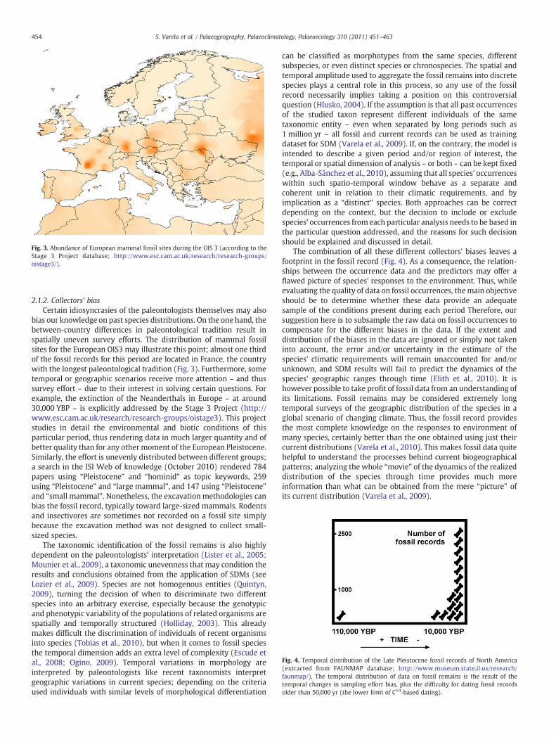
Fig. 3. Abundance of European mammal fossil sites during the OIS 3 (according to theStage 3 Project database; http://www.esc.cam.ac.uk/research/research-groups/oistage3/).

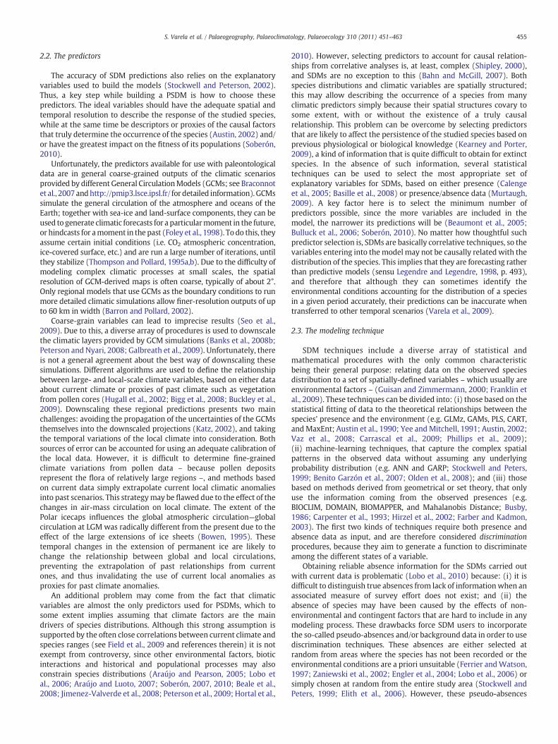
Fig. 4. Temporal distribution of the Late Pleistocene fossil records of North America(extracted from FAUNMAP database; http://www.museum.state.il.us/research/faunmap/). The temporal distribution of data on fossil remains is the result of thetemporal changes in sampling effort bias, plus the difficulty for dating fossil recordsolder than 50,000 yr (the lower limit of C14-based dating).

454 S. Varela et al. / Palaeogeography, Palaeoclimatology, Palaeoecology 310 (2011) 451–463

2.1.2. Collectors' biasCertain idiosyncrasies of the paleontologists themselves may also

bias our knowledge on past species distributions. On the one hand, thebetween-country differences in paleontological tradition result inspatially uneven survey efforts. The distribution of mammal fossilsites for the European OIS3 may illustrate this point; almost one thirdof the fossil records for this period are located in France, the countrywith the longest paleontological tradition (Fig. 3). Furthermore, sometemporal or geographic scenarios receive more attention – and thussurvey effort – due to their interest in solving certain questions. Forexample, the extinction of the Neanderthals in Europe – at around30,000 YBP – is explicitly addressed by the Stage 3 Project (http://www.esc.cam.ac.uk/research/research-groups/oistage3). This projectstudies in detail the environmental and biotic conditions of thisparticular period, thus rendering data in much larger quantity and ofbetter quality than for any other moment of the European Pleistocene.Similarly, the effort is unevenly distributed between different groups;a search in the ISI Web of knowledge (October 2010) rendered 784papers using “Pleistocene” and “hominid” as topic keywords, 259using “Pleistocene” and “large mammal”, and 147 using “Pleistocene”and “small mammal”. Nonetheless, the excavation methodologies canbias the fossil record, typically toward large-sized mammals. Rodentsand insectivores are sometimes not recorded on a fossil site simplybecause the excavation method was not designed to collect small-sized species.

The taxonomic identification of the fossil remains is also highlydependent on the paleontologists' interpretation (Lister et al., 2005;Mounier et al., 2009), a taxonomic unevenness that may condition theresults and conclusions obtained from the application of SDMs (seeLozier et al., 2009). Species are not homogenous entities (Quintyn,2009), turning the decision of when to discriminate two differentspecies into an arbitrary exercise, especially because the genotypicand phenotypic variability of the populations of related organisms arespatially and temporally structured (Holliday, 2003). This alreadymakes difficult the discrimination of individuals of recent organismsinto species (Tobias et al., 2010), but when it comes to fossil speciesthe temporal dimension adds an extra level of complexity (Escude etal., 2008; Ogino, 2009). Temporal variations in morphology areinterpreted by paleontologists like recent taxonomists interpretgeographic variations in current species; depending on the criteriaused individuals with similar levels of morphological differentiation

can be classified as morphotypes from the same species, differentsubspecies, or even distinct species or chronospecies. The spatial andtemporal amplitude used to aggregate the fossil remains into discretespecies plays a central role in this process, so any use of the fossilrecord necessarily implies taking a position on this controversialquestion (Hlusko, 2004). If the assumption is that all past occurrencesof the studied taxon represent different individuals of the sametaxonomic entity – even when separated by long periods such as1 million yr – all fossil and current records can be used as trainingdataset for SDM (Varela et al., 2009). If, on the contrary, the model isintended to describe a given period and/or region of interest, thetemporal or spatial dimension of analysis – or both – can be kept fixed(e.g., Alba-Sánchez et al., 2010), assuming that all species' occurrenceswithin such spatio-temporal window behave as a separate andcoherent unit in relation to their climatic requirements, and byimplication as a “distinct” species. Both approaches can be correctdepending on the context, but the decision to include or excludespecies' occurrences from each particular analysis needs to be based inthe particular question addressed, and the reasons for such decisionshould be explained and discussed in detail.

The combination of all these different collectors' biases leaves afootprint in the fossil record (Fig. 4). As a consequence, the relation-ships between the occurrence data and the predictors may offer aflawed picture of species' responses to the environment. Thus, whileevaluating the quality of data on fossil occurrences, themain objectiveshould be to determine whether these data provide an adequatesample of the conditions present during each period Therefore, oursuggestion here is to subsample the raw data on fossil occurrences tocompensate for the different biases in the data. If the extent anddistribution of the biases in the data are ignored or simply not takeninto account, the error and/or uncertainty in the estimate of thespecies' climatic requirements will remain unaccounted for and/orunknown, and SDM results will fail to predict the dynamics of thespecies' geographic ranges through time (Elith et al., 2010). It ishowever possible to take profit of fossil data from an understanding ofits limitations. Fossil remains may be considered extremely longtemporal surveys of the geographic distribution of the species in aglobal scenario of changing climate. Thus, the fossil record providesthe most complete knowledge on the responses to environment ofmany species, certainly better than the one obtained using just theircurrent distributions (Varela et al., 2010). This makes fossil data quitehelpful to understand the processes behind current biogeographicalpatterns; analyzing the whole “movie” of the dynamics of the realizeddistribution of the species through time provides much moreinformation than what can be obtained from the mere “picture” ofits current distribution (Varela et al., 2009).

455S. Varela et al. / Palaeogeography, Palaeoclimatology, Palaeoecology 310 (2011) 451–463

2.2. The predictors

The accuracy of SDM predictions also relies on the explanatoryvariables used to build the models (Stockwell and Peterson, 2002).Thus, a key step while building a PSDM is how to choose thesepredictors. The ideal variables should have the adequate spatial andtemporal resolution to describe the response of the studied species,while at the same time be descriptors or proxies of the causal factorsthat truly determine the occurrence of the species (Austin, 2002) and/or have the greatest impact on the fitness of its populations (Soberón,2010).

Unfortunately, the predictors available for use with paleontologicaldata are in general coarse-grained outputs of the climatic scenariosprovided by different General CirculationModels (GCMs; see Braconnotet al., 2007 andhttp://pmip3.lsce.ipsl.fr/ for detailed information). GCMssimulate the general circulation of the atmosphere and oceans of theEarth; together with sea-ice and land-surface components, they can beused to generate climatic forecasts for a particularmoment in the future,or hindcasts for amoment in the past (Foley et al., 1998). To do this, theyassume certain initial conditions (i.e. CO2 atmospheric concentration,ice-covered surface, etc.) and are run a large number of iterations, untilthey stabilize (Thompson and Pollard, 1995a,b). Due to the difficulty ofmodeling complex climatic processes at small scales, the spatialresolution of GCM-derived maps is often coarse, typically of about 2°.Only regional models that use GCMs as the boundary conditions to runmore detailed climatic simulations allow finer-resolution outputs of upto 60 km in width (Barron and Pollard, 2002).

Coarse-grain variables can lead to imprecise results (Seo et al.,2009). Due to this, a diverse array of procedures is used to downscalethe climatic layers provided by GCM simulations (Banks et al., 2008b;Peterson and Nyari, 2008; Galbreath et al., 2009). Unfortunately, thereis not a general agreement about the best way of downscaling thesesimulations. Different algorithms are used to define the relationshipbetween large- and local-scale climate variables, based on either dataabout current climate or proxies of past climate such as vegetationfrom pollen cores (Hugall et al., 2002; Bigg et al., 2008; Buckley et al.,2009). Downscaling these regional predictions presents two mainchallenges: avoiding the propagation of the uncertainties of the GCMsthemselves into the downscaled projections (Katz, 2002), and takingthe temporal variations of the local climate into consideration. Bothsources of error can be accounted for using an adequate calibration ofthe local data. However, it is difficult to determine fine-grainedclimate variations from pollen data – because pollen depositsrepresent the flora of relatively large regions –, and methods basedon current data simply extrapolate current local climatic anomaliesinto past scenarios. This strategymay be flawed due to the effect of thechanges in air-mass circulation on local climate. The extent of thePolar icecaps influences the global atmospheric circulation—globalcirculation at LGM was radically different from the present due to theeffect of the large extensions of ice sheets (Bowen, 1995). Thesetemporal changes in the extension of permanent ice are likely tochange the relationship between global and local circulations,preventing the extrapolation of past relationships from currentones, and thus invalidating the use of current local anomalies asproxies for past climate anomalies.

An additional problem may come from the fact that climaticvariables are almost the only predictors used for PSDMs, which tosome extent implies assuming that climate factors are the maindrivers of species distributions. Although this strong assumption issupported by the often close correlations between current climate andspecies ranges (see Field et al., 2009 and references therein) it is notexempt from controversy, since other environmental factors, bioticinteractions and historical and populational processes may alsoconstrain species distributions (Araújo and Pearson, 2005; Lobo etal., 2006; Araújo and Luoto, 2007; Soberón, 2007, 2010; Beale et al.,2008; Jimenez-Valverde et al., 2008; Peterson et al., 2009; Hortal et al.,

2010). However, selecting predictors to account for causal relation-ships from correlative analyses is, at least, complex (Shipley, 2000),and SDMs are no exception to this (Bahn and McGill, 2007). Bothspecies distributions and climatic variables are spatially structured;this may allow describing the occurrence of a species from manyclimatic predictors simply because their spatial structures covary tosome extent, with or without the existence of a truly causalrelationship. This problem can be overcome by selecting predictorsthat are likely to affect the persistence of the studied species based onprevious physiological or biological knowledge (Kearney and Porter,2009), a kind of information that is quite difficult to obtain for extinctspecies. In the absence of such information, several statisticaltechniques can be used to select the most appropriate set ofexplanatory variables for SDMs, based on either presence (Calengeet al., 2005; Basille et al., 2008) or presence/absence data (Murtaugh,2009). A key factor here is to select the minimum number ofpredictors possible, since the more variables are included in themodel, the narrower its predictions will be (Beaumont et al., 2005;Bulluck et al., 2006; Soberón, 2010). No matter how thoughtful suchpredictor selection is, SDMs are basically correlative techniques, so thevariables entering into themodel may not be causally related with thedistribution of the species. This implies that they are forecasting ratherthan predictive models (sensu Legendre and Legendre, 1998, p. 493),and therefore that although they can sometimes identify theenvironmental conditions accounting for the distribution of a speciesin a given period accurately, their predictions can be inaccurate whentransferred to other temporal scenarios (Varela et al., 2009).

2.3. The modeling technique

SDM techniques include a diverse array of statistical andmathematical procedures with the only common characteristicbeing their general purpose: relating data on the observed speciesdistribution to a set of spatially-defined variables – which usually areenvironmental factors – (Guisan and Zimmermann, 2000; Franklin etal., 2009). These techniques can be divided into: (i) those based on thestatistical fitting of data to the theoretical relationships between thespecies' presence and the environment (e.g. GLMz, GAMs, PLS, CART,andMaxEnt; Austin et al., 1990; Yee and Mitchell, 1991; Austin, 2002;Vaz et al., 2008; Carrascal et al., 2009; Phillips et al., 2009);(ii) machine-learning techniques, that capture the complex spatialpatterns in the observed data without assuming any underlyingprobability distribution (e.g. ANN and GARP; Stockwell and Peters,1999; Benito Garzón et al., 2007; Olden et al., 2008); and (iii) thosebased on methods derived from geometrical or set theory, that onlyuse the information coming from the observed presences (e.g.BIOCLIM, DOMAIN, BIOMAPPER, and Mahalanobis Distance; Busby,1986; Carpenter et al., 1993; Hirzel et al., 2002; Farber and Kadmon,2003). The first two kinds of techniques require both presence andabsence data as input, and are therefore considered discriminationprocedures, because they aim to generate a function to discriminateamong the different states of a variable.

Obtaining reliable absence information for the SDMs carried outwith current data is problematic (Lobo et al., 2010) because: (i) it isdifficult to distinguish true absences from lack of informationwhen anassociated measure of survey effort does not exist; and (ii) theabsence of species may have been caused by the effects of non-environmental and contingent factors that are hard to include in anymodeling process. These drawbacks force SDM users to incorporatethe so-called pseudo-absences and/or background data in order to usediscrimination techniques. These absences are either selected atrandom from areas where the species has not been recorded or theenvironmental conditions are a priori unsuitable (Ferrier andWatson,1997; Zaniewski et al., 2002; Engler et al., 2004; Lobo et al., 2006) orsimply chosen at random from the entire study area (Stockwell andPeters, 1999; Elith et al., 2006). However, these pseudo-absences

456 S. Varela et al. / Palaeogeography, Palaeoclimatology, Palaeoecology 310 (2011) 451–463

should be used with caution (Lobo and Tognelli, 2011) because theway they are selected has a great influence on the geographicrepresentation of the distribution of the species that is finally obtained(Chefaoui and Lobo, 2008; Anderson and Raza, 2010; Lobo et al.,2010).

Depending on the protocol used to select pseudo-absences (or thedecision to use only presences), the geographical response describedby SDM results can oscillate between the realized and the potentialdistribution of the species (Jimenez-Valverde et al., 2008; Colwell andRangel, 2009; Soberón and Nakamura, 2009). In fact, backgroundabsence data selected at random may be appropriate to estimate theprobability of use of a resource against its availability in order toidentify environmental or habitat preferences (i.e., Resource SelectionFunctions; Boyce and McDonald, 1999), but not to model realized orpotential distributions (McDonald et al., 2002). Choosing absence datafor SDMs that are going to be projected into different temporalscenarios separated by many generations presents additional prob-lems. The common spatial, collector and taphonomic biases ofpaleontological data hamper their use for the validation of SDMscalibrated with current data. Importantly, the same species will showdifferent realizeddistributions in eachperioddue tonon-environmentaland contingent effects that prevent it fromholding populations inmanysuitable areas. This prevents the direct use of absence information tocalibrate PSDMs; even if these factors can be included in the modelingprocess for a given temporal scenario, there is no guarantee that theireffect would be similar in a different period.

Based on the conceptual and methodological drawbacks describedabove, in this article we recommend not using discrimination orcorrelative SDM techniques to model fossil data. This leaves presencerecords from fossil remains as the only reliable source of informationon the past distribution of a species. These data provide valuableinformation on the environmental conditions for which the speciesmay have had a positive net rate of demographic growth. The locationof the regions with similar conditions to those where the speciesoccurred offers a preliminary picture of its potential distribution—theplaces that couldbe inhabited by the species in the absenceof significantdispersal limitations, local extinctions, competitive exclusion and/orsurvey biases (Jimenez-Valverde et al., 2008; Colwell and Rangel, 2009;Soberón and Nakamura, 2009; Lobo et al., 2010).

Establishing a robust methodological framework for the use ofGCM-based projections of past climate and PSDMs in the emergingfield of paleobiogeography should be rooted in careful methodologicalchoices. Although complex methods provide powerful ways of fittingthe data, they often provide responses that are too narrow for theenvironment (Jimenez-Valverde et al., 2008). Choices should insteadbe based on the capacity of SDM techniques to account for the species'responses to climatic and non-climatic factors for a given period andprovide reliable projections of these responses to other moments oftime. These conditions are met by the methods based on geometricalor set theory, which are safe from the errors caused by the use ofabsence data in the training dataset. Given the concerns above, andthe problems found when using presence/absence approaches toestimate the past distribution of species (Varela et al., 2009), we arguethat although presence/absence SDMs may be suitable for describingthe distribution of a species in a single period, they are certainly notadequate for predicting the species' response throughout severalscenarios of changing climate. Thus, we stress that discriminationtechniques and similar procedures should be avoided for estimatingthe past distribution of species, because they are quite likely tounderestimate their potential distribution (see Jiménez-Valverde etal., 2011).

The different SDM techniques available to predict speciesdistributions from presence-only data (Tsoar et al., 2007; Calengeand Basille, 2008) are based on the estimation of both the species'tolerance range and the species' optimum conditions according to theselected environmental predictors. The potential distribution of a

species can be partially estimated from observed occurrences bymeans of a Multidimensional Enveloping procedure (MDE; see Busby,1986), taking into account that: (i) the species may be able to surviveoutside the environmental conditions provided by the observedlocalities (Soberón and Peterson, 2005; Soberón and Nakamura, 2009;Varela et al., 2009); and (ii) the species will only inhabit a portion ofits fundamental niche that depends on the readily availableenvironmental space (Jackson and Overpeck, 2000). MDE can beused to generate either binary or continuous suitability maps. Binarygeographical projections (i.e., suitable versus unsuitable localities)can be obtained by estimating the extreme maximum and minimumenvironmental values that may be inhabited by the species, to thendelimit the suitable conditions in the multidimensional environmen-tal space bymeans of a generalized intersection procedure, and finallytransfer these conditions to the geographical space.

In contrast toMDE, continuous representations of suitability requireestimating both the species' tolerances and its environmental optimum,to provide a gradient from more to less favorable conditions.Estimations of the environmental tolerance are highly dependent onthe inclusion of extreme occurrences, so reliable information onpresences near the physiological limits of the species is very importantto estimate its potential distribution. In the specific case of paleonto-logical data, we also recommend training PSDMswith asmuch past andrecent information on presences as possible, thus maximizing theproportion of the full spectrum of environmental conditions inhabitedby the species that is sampled by the data (Varela et al., 2009).

If the aim is to obtain information about the variability in the climaticsuitability of the species, we suggest using a measure of theenvironmental distance from each site to the optimum, such as thescale-invariant Mahalanobis Distance (Kadmon et al., 2003; Allouche etal., 2008; Calenge et al., 2008; Etherington et al., 2009). Needless to say,the selection of the climatic optimum is a key point in this case, since itmay also highly influence the obtained results. Although MDE caninclude the distribution of the data within the variables while modelingclimatic suitability (Ruegg et al., 2006), this approachwill only produceaccurate results when using complete and unbiased presence data sets.In the same manner, the mean, median or any other central tendencymeasure can only provide good estimations of the species optimumwhen the data set constitutes a reliable subsample of the species'requirements (Nogues-Bravo et al., 2008). Therefore,we arguehere thatwhen studying paleontological data it is important to emphasize therole of environmental limits (Huston, 2002) while at the same timeavoiding the effect of bias in current and past fossil distribution data.Wethus recommend calculating the central point of the n-dimensionalenvironmental space used by the species as the central point of itsamplitude ([maximum−minimum]/2+minimum), to ensure that theassumed optimum environmental conditions are equidistant from theextreme values (Varela et al., 2010).

3. Former species distribution modeling applications inpaleontology

During our literature search for applications of SDMs in paleontolog-ical research (ISI Web of knowledge, September 2010; Search criteria:species distribution model+fossil, species distribution model+lastglacial maximum, species distribution model+Pleistocene) we found atotal of forty-two papers (Tables 1 and 2; see also Nogues-Bravo, 2009;Svenning et al., 2011). These works study changes in the distribution ofspecies from a wide range of taxa, including plants, vertebrates andinsects (Jakobet al., 2009; Jezkovaet al., 2009;Marskeet al., 2009), aswellas changes in the areas occupied by forests or biomes (Bonaccorso et al.,2006; Carstens and Knowles, 2007; Hilbert et al., 2007). The extent ofanalysis is also heterogeneous, varying from regional (e.g. IberianPeninsula; Benito Garzón et al., 2007) to continental (e.g. Europe, NorthAmerica; Banks et al., 2006) or even global (e.g. Yesson and Culham,2006). In this sectionwe review the occurrence data, predictors and SDM

Table 1Summary of the occurrence data used in the forty-two papers using Paleo-Species Distribution Modeling analyzed in this work.

Geographic extent Climatic variables SDM technique References

GCM past Downscaling/variables Resolution

Iberian Peninsula CCSM, MIROC Current local climate to estimate past local climate 200 m MaxEnt Alba-Sánchez et al. (2010)Western Europe PMIP2 protocol Refined grid over Europe 60 km GARP Banks et al. (2008a)Western Europe PMIP1 protocol Refined grid over Europe 60 km GARP Banks et al. (2008b)Western Europe and North America HadCM3 – 100–200 km GARP Banks et al. (2006)Switzerland – Use current climate to estimate past climate 1 km LGMz Baumann et al. (2005)Iberian Peninsula ECHAM3, UGAMP Current local climate to estimate past local climate – Random forest Benito Garzón et al. (2007)North Atlantic Ocean GCM Interpolation 5′ MaxEnt, “ecophysiologic ranges’ Bigg et al. (2008)Amazon Basin HadCM3 – 0.1° GARP Bonaccorso et al. (2006)New Zealand – Based on current climate and indirect data 100 m MaxEnt Buckley et al. (2009)Iberian Peninsula ECHAM3 Anomaly data and interpolating by thin-plane splines 1 km Random forest Calleja et al. (2009)South America ECHAM3 Bilinear interpolation 30″ MaxEnt, Bioclim Carnaval and Moritz (2008)Brazilian Atlantic rainforest – – – MaxEnt Carnaval et al. (2009)Western North America CCSM3 Interpolation – MaxEnt Carstens and Knowles (2007)Central Europe CCSM Current local climate to estimate past local climate 10′ Bioclim Depraz et al. (2008)South Africa – Use current climate to estimate past climate 15″ Bioclim Eeley et al. (1999)Eurasia S3P, LMDZHR Current local climate to estimate past local climate 30″ MaxEnt, Bioclim Flojgaard et al. (2009)North America CCSM3, MIROC Current local climate to estimate past local climate 2.5′ MaxEnt Galbreath et al. (2009)America ECHAM3 Current local climate to estimate past local climate 1 km MaxEnt, Bioclim, Domain, GAM Hijmans and Graham (2006)North Queensland, Australia – Use current climate to estimate past climate 80 m Bioclim Hugall et al. (2002)North Queensland, Australia – Use current climate to estimate past climate 1 ha Artificial neural networks Hilbert et al. (2007)Eastern North America MIROC Interpolation 2.5′ MaxEnt Jezkova et al. (2009)South America CCSM, MIROC Interpolation 0,01°–0,04° GARP Jakob et al. (2009)North America CCSM3 Interpolation 1′ MaxEnt Knowles et al. (2007)North America – Based on fossil and sedimentary data 1° GARP Araújo and New (2007, 2009)New Zealand – Use current climate to estimate past climate 100 m MaxEnt Marske et al. (2009)North America HadCM2 Resampled 0.1° GARP Martínez-Meyer and Peterson (2006)North America – Use current climate to estimate past climate – GARP Martínez-Meyer et al. (2004)Australian wet tropics – Estimated from pollen – Averaged GLMz Moussalli et al. (2009)Eurasia GENESIS – 2° Mahalanobis Distances, MaxEnt, Bioclim Nogues-Bravo et al. (2008)Europe UBRIS-HadCM3 Current local climate to estimate past local climate 1 km Boosted regression trees Pearman et al. (2008)North America HadCM Current local climate to estimate past local climate 0.1° GARP Peterson et al. (2004)Central and South America MIROC, CCSM Current local climate to estimate past local climate 0.04° GARP, MaxEnt Peterson and Nyari (2008)Europe and the Mediterranean ECHAM3, UGAMP Current local climate to estimate past local climate 100 km MaxEnt Rodriguez-Sanchez and Arroyo (2008)America ECHAM Current local climate to estimate past local climate 10 km Bioclim Ruegg et al. (2006)Central and South America ECHAM Current local climate to estimate past local climate 100 km MaxEnt Solomon et al. (2008)Europe S3P, LMDZHR Refined grid over Europe 60 km MaxEnt, Bioclim Svenning et al. (2008)Eurasia and Africa GENESIS – 4.5°×7.5° LGMz, Bioclim Varela et al. (2009)Eurasia and Africa GENESIS – 2° Mahalanobis Distances, Bioclim Varela et al. (2010)Indiana and Ohio (United States of A.) – Interpolation-ordinary kriging based on sedimentary data 15′ GARP Walls and Stigall (2011)North America CCSM, MIROC Current local climate to estimate past local climate 2.5′ MaxEnt, GARP Waltari et al. (2007)North America CCSM, MIROC Current local climate to estimate past local climate 2.5′ MaxEnt, GARP Waltari and Guralnick (2009)Global and Australia BRIDGE – 2° Bioclim Yesson and Culham (2006)

457S.V

arelaet

al./Palaeogeography,Palaeoclim

atology,Palaeoecology310

(2011)451

–463

Table 2Geographic extent, General CirculationModels projected to the past, and downscalingmethodologies used to construct the predictors of the Paleo-Species DistributionModels in theforty-two papers analyzed here.

Training data References

Current data Fossil data Target species

Species distribution maps – Abies spp. Alba-Sánchez et al. (2010)Georeferenced occurrences Georeferenced fossil sites Rangifer tarandus, Cervus elaphus Banks et al. (2008a)– Georeferenced archeological sites Homo sapiens Banks et al. (2008b)– Georeferenced archeological sites Homo sapiens Banks et al. (2006)Georeferenced occurrences Georeferenced archeological sites Rupicapra rupicapra Baumann et al. (2005)Species distribution maps – 19 tree species Benito Garzón et al. (2007)Georeferenced occurrences – Gadus spp. Bigg et al. (2008)Georeferenced occurrences – 6 trees, 11 birds Bonaccorso et al. (2006)Georeferenced occurrences – Argosarchus horridus Buckley et al. (2009)Georeferenced occurrences – Prunus lusitanica Calleja et al. (2009)Georeferenced occurrences – Forest spp. Carnaval and Moritz (2008)Georeferenced occurrences – Hypsiboas spp. Carnaval et al. (2009)Georeferenced occurrences – Frogs, trees and mammals Carstens and Knowles (2007)Georeferenced occurrences – Trochulus villosus Depraz et al. (2008)Species distribution maps – Indigenous forests Eeley et al. (1999)Species distribution maps – Rodents Flojgaard et al. (2009)Georeferenced occurrences – Ochotona princeps Galbreath et al. (2009)Species distribution maps – 100 plant spp. Hijmans and Graham (2006)Georeferenced occurrences – Gnarosophia bellendenkerensis Hugall et al. (2002)Species distribution maps Forest classes Hilbert et al. (2007)Georeferenced occurrences – Chaetodipus penicillatus Jezkova et al. (2009)Georeferenced occurrences – Hordeum species (Poaceae) Jakob et al. (2009)Georeferenced occurrences – Melanoplus marshalli Knowles et al. (2007)– Georeferenced fossil sites Subfamily Equinae Maguire and Stigall (2009)Georeferenced occurrences – Agyrtodes labralis Marske et al. (2009)Georeferenced occurrences Georeferenced fossil sites 8 tree species Martínez-Meyer and Peterson (2006)Georeferenced occurrences Georeferenced fossil sites 23 mammal species Martinez-Meyer et al. (2004)Georeferenced occurrences – Saproscincus spp. Moussalli et al. (2009)– Georeferenced fossil sites Mammuthus primigenius Nogues-Bravo et al. (2008)Species distribution maps Georeferenced fossil sites tree spp. Pearman et al. (2008)Georeferenced occurrences – Aphelocoma jays Peterson et al. (2004)Georeferenced occurrences – Schiffornis sp. Peterson and Nyari (2008)Georeferenced occurrences Georeferenced fossil sites Laurus sp. Rodriguez-Sanchez and Arroyo (2008)Georeferenced occurrences – Catharus ustulatus Ruegg et al. (2006)Georeferenced occurrences – Atta spp. Solomon et al. (2008)Species distribution maps – 22 tree spp. Svenning et al. (2008)Georeferenced occurrences – Crocuta crocuta Varela et al. (2009)Georeferenced occurrences Georeferenced fossil sites Crocuta crocuta Varela et al. (2010)– Georeferenced fossil sites 8 brachiopod species Walls and Stigall (2011)Georeferenced occurrences – 20 terrestrial vertebrates Waltari et al. (2007)Georeferenced occurrences – 13 mammal species Waltari and Guralnick (2009)Georeferenced occurrences Georeferenced fossil sites Drossera sp. Yesson and Culham (2006)

458 S. Varela et al. / Palaeogeography, Palaeoclimatology, Palaeoecology 310 (2011) 451–463

techniques used in these papers to provide a synthesis of the basiccharacteristics of the Paleo-Species Distribution Modeling applicationsconducted so far. This complements the former reviewsbyNogues-Bravo(2009) andSvenninget al. (2011)bydiscussing indetail the limitationsofformer PSDM papers based on the theoretical and practical needs of thistype of studies discussed above.

3.1. The occurrence data

The training datasets include current species' occurrences in 29 ofthe 42 papers, and current species distribution maps in eight papers;only five papers are based just on georeferenced fossil records andanother eight use both current and past occurrences (see Table 1). Inspite of such variety of data types, these papers rarely comment on thegeographic and temporal extent of the data, the completeness of thepresence data or how absence data was selected (but see Nogues-Bravo et al., 2008 and Varela et al., 2010). The geographic extent of thetraining data is usually the region where the model will be projected;in some papers this extent covers the total distribution area of thespecies but in others it does not (Banks et al., 2008a), a practice thatcan be amajor issue for the reliability of PSDMs. Failing to include data

from the entire geographic distribution of a species can result insampling a spuriously narrow range of environmental tolerance,which ultimately results in an underestimation of its potentialdistribution (Thuiller et al., 2004; Sánchez-Fernández et al., 2011).

Importantly, the majority of PSDM applications have so far beentrained using only a single temporal scenario (Table 1). In almostthree quarters of the studies (29 cases) the SDM was calibrated usingonly the current distribution of the species (see Table 1), a practicethat may fail to represent its past distribution (Varela et al., 2009). Infact, the only two papers that evaluate the assumption that theprojections from a PSDM calibrated in a given period are able topredict the presence of the species in a different moment of time givemixed results; while Nogués-Bravo et al. (2008) found that thetransferability between periods provided adequate results, Varela etal. (2009) found inconsistency between the projections for differentperiods. This lack of evaluation of the assumption of temporaltransferability is further complicated by the use of absence data totrain the models in 36 papers (see Table 2), 27 of which use eitherMaxEnt or GARP with background absences. As discussed above, theuse of these absence data for training the models prevents them fromidentifying the potential distribution of the species.

459S. Varela et al. / Palaeogeography, Palaeoclimatology, Palaeoecology 310 (2011) 451–463

3.2. Predictor variables

Twenty-four out of the 42 papers analyzed downscale the climaticpredictors (see Table 2). Fifteen of these studies use the spatialpatterns, amplitude and sign of current climatic anomalies at the localscale to construct fine-scale climatic layers, assuming that they areidentical through time. Seven papers adopt an even simpler strategyand construct the variables describing past climate simply by addingor subtracting certain values to the current climatic layers. Asdiscussed above, both methods are likely to include significant errorsin the climatic predictors. Nevertheless, the lack of a standard fordownscaling past climate scenarios includes a source of variability inthe predictors between studies, that hampers the direct comparison oftheir results, evenwhen they refer to the same geographic area and/ortemporal scenario.

Although it is well known that the number and identity ofpredictors have a major influence on SDM results, few papers choosethese independent variables based on an ecologically meaningfulstrategy. In fact, the predictors used in the analysis are generallychosen on the basis of their easy availability. As a result, the 19WorldClim variables (available at http://www.worldclim.org/) are themost used predictors for current time. GCM-derived climatic layers forpast scenarios are more difficult to access, and therefore a diversearray of GCMs has been used for this task. Given the difficulty ofextrapolating GCMs to the past and the limitations in projectingcomplex aspects of climate, Annual Mean Temperature and AnnualPrecipitation are also the predictors most commonly included inPSDMs. There are, however, some exceptions to these opportunisticstrategies, and in a few studies the selection of predictors is based onthe researcher's knowledge about the specific factors that may affectthe distribution of the species (e. g., Bigg et al., 2008;Walls and Stigall,2011).

3.3. Modeling techniques

Most of the analyzed studies use discrimination techniques whichincorporate some kind of pseudoabsence data to estimate the pastdistribution of species, including MaxEnt, GLMz, GAM, GARP, RF, BRTand ANN (see Table 2). From these, MaxEnt is the most popular, beingused in nearly half of the papers (19 cases), followed by GARP (13cases). Geometrical or set theory based techniques are used in 12papers; all of them use Bioclim, together with Mahalanobis Distancesin two occasions (Nogues-Bravo et al., 2008; Varela et al., 2009).

3.4. Problems and limitations of former PSDM approaches

A diverse array of methods has been used so far to estimate thepast distribution of species. According to the conceptual andmethodological issues discussed above, we suspect that most formerPSDM approaches could be overestimating the role that climaticchanges had on past species' range shifts and/or extinction events. Ingeneral, the choice of the distributional data used to train the modelsis based only on the type of data available (current, fossil, or both),rather than on their adequacy for the question at hand. These worksmake the implicit assumption that the available information about thespecies is sufficient to estimate its climatic requirements andtherefore to calibrate a model that can safely be projected to thepast. Unfortunately, we believe that this assumption may prove to befalse in many cases. The limited quality of the data on both recent andfossil occurrences may often fail to represent the full spectrum ofclimatic conditions at which the species can inhabit, so given howSDM results depend on the data used to train them, current commonpractice in PSDM could be regularly leading to underestimate thegeographic ranges of the species in different periods of time. Theprobability of underestimating the species' potential requirementswill, however, diminish if the occurrences in the training dataset

cover the entire geographic and temporal extent in which the specieshas lived, as well as if the inclusion of any kind of absence data isavoided (see above, and also Jimenez-Valverde et al., 2008).

We also advocate that PSDMs should be built based on a carefulselection of climatic predictors, a step that is commonly overlooked inthe reviewed literature. To do this, and in the absence of previousknowledge on the actual species' requirements, we recommend usingmultivariate niche description techniques such as Ecological-NicheFactor Analysis (ENFA; Hirzel et al., 2002; Basille et al., 2008) to selectthose variables with higher probabilities of being causally related tothe species' occurrences. Also, the projections of PSDMs at differentmoments of time should be cross-examined whenever possible, toensure that models calibrated with data from a certain period areable to describe the occurrence of the species in other momentsof time.

Finally, we want to stress that the SDM techniques used should beappropriate to the questions posed. Different SDM proceduresproduce wider or narrower geographic predictions and consequentlythey can have a profound impact in the biological interpretation of theresults (Jimenez-Valverde et al., 2008). We thus believe that in theabsence of any supplementary information about the species' climaticrequirements, the methodological approach used for PSDMs needs tobe conservative. While data for these analyses is typically composedof samples of the species' geographic range at different moments oftime, these ranges are dynamic and vary as a consequence of theinteractions between the potential distribution of the species andboth climatic and non-climatic factors. Given the importance of non-climatic factors in preventing species from occurring in climaticallysuitable areas, discrimination techniques based on absence informa-tion should be discarded for the estimation of the climatic niche andthe past distribution of species, because they would underestimate itspotential distribution. In this context, we think that themost adequateoption to predict the potential distribution of a species through timeto use the more conservative multidimensional climatic envelopes,such as Bioclim. Similarly, Mahalanobis Distance would be appropri-ate when the aim is to estimate the climatic suitability based on ahypothetical climatic optimum.

4. Future prospects for paleobiogeography

The generalization of Paleo-Species Distribution Modeling ap-proaches has great potential for generating new paleontologicalinformation and hypotheses in the forthcoming years. To take fullprofit of such potential it is however crucial: (i) to create a globaldatabase to compile all distributional information available for thePleistocene; (ii) to develop high resolution climatic layers for differentpast scenarios by means of a widely-agreed on standardizeddownscaling protocol; and (iii) the in-depth investigation of thenature and temporal variation of species–climate relationships, aswell as of which SDM methodologies provide the most adequatesimulations of these changing relationships.

The analysis of the Pleistocene distribution of any species impliesusing data from different fossil sites. Therefore, one of the first goalsfor the development of modern paleobiogeography should be toestablish a global open-access database, similar to the ones availablefor current species, such as the GBIF network (http://www.gbif.org/).Some initiatives are already aiming to provide databases on fossil dataon the Internet, including the Paleobiology Database (http://www.paleodb.org/cgi-bin/bridge.pl), Faunmap (http://www.museum.state.il.us/research/faunmap/), Neotoma (http://www.neotomadb.org/),the printed compilation of data in Evolution of Tertiary Mammals inNorth America (Janis et al., 2005, 2008), Stage Three Project (http://www.esc.cam.ac.uk/research/research-groups/oistage3/) and NOW(Neogene Old World database; http://www.helsinki.fi/science/now/).However, several points need to be improved in these databases. First,the available information about fossil dating is extremely broad. As an

460 S. Varela et al. / Palaeogeography, Palaeoclimatology, Palaeoecology 310 (2011) 451–463

example, Homo antecessor is roughly assigned to the Pleistocene (1.810to 0.011 Ma) (query on The Paleobiology Database) when it has beendated by paleomagnetism as being not older than 780 Ma, and assignedto the end of the Earlier Pleistocene using ESR andU-series (Falgueres etal., 1999). Second, the temporal and spatial scopes of thesedatabases arelimited. For example, the Stage 3 Project compiles European fossil sitesprevious to the Last Glacial Maximum, and FAUNMAP is geographicallyrestricted to North America. Third, all of these databases have rigidtaxonomic classifications. Pleistocene mammal taxonomy has beenchanged in the light of new evidence (Alroy, 2003) and fossil recordscould be reclassified in the future due to the appearance new evidencebased on ancient DNA studies or any other new technology. Therefore,any durable database should allow using as many taxonomic classifi-cations as would be necessary, providing taxonomic fields that alloweventual changes in the systematic of the group or the reassignment ofspecific fossil remains to different taxa in the light of future revisions.The experience of neosystematicians in building standards for biodi-versity information (see the most updated information on theTaxonomic Database Working Group at http://www.tdwg.org/) willmake thedesignof suchapaleodistributionaldatabase relatively easy. Inany case, a good knowledge on the species and/or taxonomic groupstudied is crucial for the taxonomic reliability of the informationgathered in the database. Similar to biodiversity databases onrecent species, an authoritative and comprehensive revision of allthe fossil remains recorded in the database and a periodic reviewof the taxonomic status of all these records are necessary for thedatabase to provide accurate information on known past species'occurrences.

Most difficulties in gathering information about the Pleistocenefossil record may be trivial. Estimating the past geographic location ofthe fossil remains should not be a significant problem, for thedistribution of landmass in the Pleistocene is similar to the currentone except for the coastline variations in relation to the glacial cycles(Peltier, 2007). Therefore, in the absence of translocations the originallocation of the remains can be safely assigned to the current loca-tion of the deposit. To guarantee the success of the database onpaleodistributional data we suggest following the philosophy of thecommunity of molecular biologists, where many journals requirethe submission of any sequence information used in the manuscriptto a unified database, the GenBank (http://www.ncbi.nlm.nih.gov/genbank/), prior to publication. A similar strategy followed byPaleontology, Ecology and Biogeography journals would help byestablishing the same philosophy in paleontological research, en-couraging researchers to upload the faunal lists of their fossil sites intoan open access database. The unified source of information thatwould be obtained with such a database will constitute a basicresource for the study of the dynamics of species ranges throughtime, the relationships between species distribution and climaticchange, or any other spatio-temporal pattern, and hence should bethe pillar of the development of modern Paleobiogeography andPaleoecology.

A unified database on the distribution of the diversity in the past isnot the sole requisite for the advancement of paleobiogeography.Species' relationshipswith climate are ultimately determining the long-term viability of local populations, and are therefore dependent on fine-scale climate patterns (Seo et al., 2009), so understanding theserelationships also requires the development of high-resolution climaticlayers for past periods. Given the uncertainty inherent to GCMs, thedevelopment of different temporal simulations may also help to assessthe robustness of PSDM results to differences in the parameterization ofthe climatic models (see also Araújo and New, 2007). Also, theprojection of GCMs to continuous temporal series of climatic projectionsrather than to key moments in time could permit the creation oftemporally dynamic models, which would in turn help to analyzehypotheses on the dispersal of species and their rangedynamics. Finally,we argue that more theoretical research is needed to understand the

species–climate relationships, following the line of research recentlyreopened by Soberón (2007, 2010) and Soberón and Nakamura (2009)(see also Kearney, 2006; Jimenez-Valverde et al., 2008 or Colwell andRangel, 2009). Such research will allow the identification of the factorsthat should be taken into account to simulate the impacts that climaticchanges have on species distributions.

5. Conclusions

The study of Pleistocene biogeography could provide newinformation about the biological consequences of climatic changes.The development of Paleo-Species Distribution Models can be acentral part of such research, benefitting from the information on thepast occurrence of species available from the fossil record, thedevelopment of Global Climate Models and their projection to pastscenarios, and the current theoretical advances on the relationshipbetween the fundamental niche of the species and their geographicaldistribution. However, three particular aspects of PSDMs must betaken into account for such development, (i) the difficulty inobtaining reliable information on species' absences; (ii) that theirresults must be extrapolated to transfer their projections over longtime periods; and (iii) the difficulty of validating these projections.Here we argue that the fossil data used to calibrate the PSDMs shouldinclude as much information as possible, trying to sample the entiregeographic and temporal extent of the species' distribution. Further-more, in our opinion, presences are the only data that are bothavailable and reliable enough to be used in PSDMs; by takingadvantage of this information it would be possible to obtain partialestimates of the climatic niche of the species that can subsequently beused to generate hypotheses on the distribution of the species inother periods. On the other hand, absence and pseudo-absence datashould be avoided, because they could add misleading informationthat would make the description of species–climate relationshipsdifficult.

Although the predictors used to build PSDMs should preferablyhave adequate resolution to describe these relationships, werecommend not to downscale the geographical projections ofGCMs using simplistic rules. Here it would be preferable to assumethat the resolution of the study is limited to coarse grains, or to waitfor the development of regional GCMs. The selection of the adequatepredictors is also a key point in the construction of PSDMs; herewe suggest using ENFA analysis to select the most biologicallymeaningful variables. Based on the restriction to presence-onlySDMs that we suggest, the most adequate PSDM methodologieswould be either (a) climatic envelopes based on the climatictolerance range of the species when the goal is to detect geographicrange shifts in relation to climatic changes; or (b) distance-basedtechniques such as Mahalanobis Distances when some continuousinformation about the climatic suitability for the species is required,although in this case the selection of the species' optimum should bediscussed and justified. By following all of these recommendationswe believe that we will be able to diminish the errors in theestimations of the potential distribution of the species, and thereforeensure that the future use of PSDMs will bring robust results andat the same time stimulate ideas in the fields of Paleoecology andPaleobiogeography.

Acknowledgments

We want to thank Raul García, María Triviño, Silvia Calvo and twoanonymous referees for their helpful suggestions and fruitful debate,Manolo Salesa and Jan van der Made for scientific and technicaladvice, and Sally Raskin for helping uswith the English. SVwas fundedby a research project of the Consejería de Educación y Ciencia deCastilla-La Mancha (POIC10-0311-0585). JH was funded by a Spanish

461S. Varela et al. / Palaeogeography, Palaeoclimatology, Palaeoecology 310 (2011) 451–463

MICINN Ramón y Cajal grant and by a Brazilian CNPq VisitingResearcher grant (400130⁄2010-6).

References

Alba-Sánchez, F., López-Saez, J.A., Benito-de Pando, B., Linares, J.C., Nieto-Lugilde, D.,López-Merino, L., 2010. Past and present potential distribution of the Iberian Abiesspecies: a phytogeographic approach using fossil pollen data and speciesdistribution models. Diversity and Distributions 16, 214–228.

Alexandrino, J., Teixeira, J., Arntzen, J.W., Ferrand, N., 2007. Historical biogeography andconservation of the golden-striped salamander (Chioglossa lusitanica) in north-western Iberia: integrating ecological, phenotypic and phylogeographic data. In:Weiss, S., Ferrand, N. (Eds.), Phylogeography of Southern European Refugia.Springer, pp. 189–205.

Allouche, O., Steinitz, O., Rotem, D., Rosenfeld, A., Kadmon, R., 2008. Incorporatingdistance constraints into species distributionmodels. Journal of Applied Ecology 45,599–609.

Alroy, J., 2003. Taxonomic inflation and body mass distributions in North Americanfossil mammals. Journal of Mammalogy 84, 431–443.

Anderson, R.P., Raza, A., 2010. The effect of the extent of the study region on GIS modelsof species geographic distributions and estimates of niche evolution: preliminarytests with montane rodents (genus Nephelomys) in Venezuela. Journal ofBiogeography 37, 1378–1393.

Andrews, P., 2006. Taphonomic effects of faunal impoverishment and faunal mixing.Palaeogeography, Palaeoclimatology, Palaeoecology 241, 572–589.

Araújo, M.B., Luoto, M., 2007. The importance of biotic interactions for modellingspecies distributions under climate change. Global Ecology and Biogeography 16,743–753.

Araújo, M.B., New, M., 2007. Ensemble forecasting of species distributions. Trends inEcology & Evolution 22, 42–47.

Araújo, M.B., Pearson, R.G., 2005. Equilibrium of species' distributions with climate.Ecography 28, 693–695.

Arroyo-Cabrales, J., Polaco, O.J., Johnson, E., 2007. An overview of the Quaternarymammals from Mexico. Courier Forschungsinstitut Senckenberg 259, 191–203.

Austin, M.P., 2002. Spatial prediction of species distribution: an interface betweenecological theory and statistical modelling. Ecological Modelling 157, 101–118.

Austin, M.P., Nicholls, A.O., Margules, C.R., 1990. Measurement of the realizedqualitative niche: environmental niches of five Eucalyptus species. EcologicalMonographs 60, 161–177.

Bahn, V., McGill, B.J., 2007. Can niche-based distribution models outperform spatialinterpolation? Global Ecology and Biogeography 16, 733–742.

Banks, W.E., d'Errico, F., Dibble, H.L., Krishtalka, L., West, D., Olszewski, D.I., Peterson, A.T.,Anderson, D.G., Gillam, J.C., Montet-White, A., Crucifix, M., Marean, C.W., Sánchez-Goñi, M.-F., Wohlfarth, B., Vanhaeran, M., 2006. Eco-cultural niche modeling: newtools for reconstructing the geography and ecology of past human populations.PaleoAnthropology 69, 68–83.

Banks, W.E., d'Errico, F., Peterson, A.T., Kageyama, M., Colombeau, G., 2008a.Reconstructing ecological niches and geographic distributions of caribou (Rangifertarandus) and red deer (Cervus elaphus) during the Last Glacial Maximum.Quaternary Science Reviews 27, 2568–2575.

Banks, W.E., d'Errico, F., Peterson, A.T., Vanhaeren, M., Kageyama, M., Sepulchre, P.,Ramstein, G., Jost, A., Lunt, D., 2008b. Human ecological niches and ranges duringthe LGM in Europe derived from an application of eco-cultural niche modeling.Journal of Archaeological Science 35, 481–491.

Barnosky, A.D., Carrasco, M.A., Davis, E.B., 2005. The impact of the species-arearelationship on estimates of paleodiversity. Plos Biology 3, 1356–1361.

Barron, E., Pollard, D., 2002. High-resolution climate simulations of oxygen isotopestage 3 in Europe. Quaternary Research 58, 296–309.

Basille, M., Calenge, C., Marboutin, E., Andersen, R., Gaillard, J.M., 2008. Assessinghabitat selection using multivariate statistics: some refinements of the ecological-niche factor analysis. Ecological Modelling 211, 233–240.

Baumann, M., Babotai, C., Schibler, J., 2005. Native or naturalized? Validating alpinechamois habitat models with archaeozoological data. Ecological Applications 15,1096–1110.

Beale, C.M., Lennon, J.J., Gimona, A., 2008. Opening the climate envelope reveals nomacroscale associations with climate in European birds. PNAS 105, 14908–14912.

Beaumont, L.J., Hughes, L., Poulsen, M., 2005. Predicting species distributions: use ofclimatic parameters in BIOCLIM and its impact on predictions of species' currentand future distributions. Ecological Modelling 186, 250–269.

Benito Garzón, M., Sánchez de Dios, R., Sáinz Ollero, H., 2007. Predictive modelling oftree species distributions on the Iberian Peninsula during the Last Glacial Maximumand Mid-Holocene. Ecography 30, 120–134.

Bermúdez de Castro, J.M., Perez-Gonzalez, A., Martinon-Torres, M., Gomez-Robles, A.,Rosell, J., Prado, L., Sarmiento, S., Carbonell, E., 2008. A new early Pleistocenehominin mandible from Atapuerca-TD6, Spain. Journal of Human Evolution 55,729–735.

Bigg, G.R., Cunningham, C.W., Ottersen, G., Pogson, G.H., Wadley, M.R., Williamson, P.,2008. Ice-age survival of Atlantic cod: agreement between palaeoecology modelsand genetics. Proceedings of the Royal Society B-Biological Sciences 275 163-U113.

Bonaccorso, E., Koch, I., Peterson, A.T., 2006. Pleistocene fragmentation of Amazonspecies' ranges. Diversity and Distributions 12, 157–164.

Bowen, D.Q., 1995. Last glacial maximum. In: Gornitz, V. (Ed.), Encyclopedia ofPaleoclimatology and Ancient Environments. Springer, Dordrecht.

Boyce, M.S., McDonald, L.L., 1999. Relating populations to habitats using resourceselection functions. Trends in Ecology & Evolution (Personal Edition) 14, 268–272.

Braconnot, P., Otto-Bliesner, B., Harrison, S., Joussaume, S., Peterschmitt, J.-Y., Abe-Ouchi, A., Crucifix, M., Driesschaert, E., Fichefet, T., Hewitt, C.D., Kageyama, M.,Kitoh, A., Laîné, A., Loutre, M.F., Marti, O., Merkel, U., Ramstein, G., Valdes, P., Weber,S.L., Yu, Y., Zhao, Y., 2007. Results of PMIP2 coupled simulations of the Mid-Holocene and Last Glacial Maximum—part 1: experiments and large-scale features.Climate of the Past 3, 261–277.

Buckley, T.R., Marske, K.A., Attanayake, D., 2009. Identifying glacial refugia in ageographic parthenogen using palaeoclimate modelling and phylogeography: theNew Zealand stick insect Argosarchus horridus (White). Molecular Ecology 18,4650–4663.

Bulluck, L., Fleishman, E., Betrus, C., Blair, R., 2006. Spatial and temporal variations inspecies occurrence rate affect the accuracy of occurrence models. Global Ecologyand Biogeography 15, 27–38.

Busby, J.R., 1986. Bioclimatic Prediction System (BIOCLIM) User's Manual Version 2.0.Australian Biological Resources Study Leaflet.

Calenge, C., Basille, M., 2008. A general framework for the statistical exploration of theecological niche. Journal of Theoretical Biology 252, 674–685.

Calenge, C., Dufour, A.B., Maillard, D., 2005. K-select analysis: a new method to analysehabitat selection in radio-tracking studies. Ecological Modelling 186, 143–153.

Calenge, C., Darmon, G., Basille, M., Loison, A., Jullien, J.M., 2008. The factorialdecomposition of the Mahalanobis distances in habitat selection studies. Ecology89, 555–566.

Calleja, J.A., Garzon, M., Ollero, H., 2009. A Quaternary perspective on the conservationprospects of the Tertiary relict tree Prunus lusitanica L. Journal of Biogeography 36,487–498.

Carnaval, A.C., Moritz, C., 2008. Historical climate modelling predicts patterns ofcurrent biodiversity in the Brazilian Atlantic forest. Journal of Biogeography 35,1187–1201.

Carnaval, A.C., Hickerson, M.J., Haddad, C.F.B., Rodrigues, M.T., Moritz, C., 2009. Stabilitypredicts genetic diversity in the Brazilian Atlantic forest hotspot. Science 323,785–789.

Carpenter, G., Gillison, A.N., Winter, J., 1993. DOMAIN. A flexible modeling procedurefor mapping potential distributions of plants and animals. Biodiversity andConservation 2, 667–680.

Carrascal, L.M., Galván, I., Gordo, O., 2009. Partial least squares regression as analternative to current regression methods used in ecology. Oikos 118, 681–690.

Carstens, B.C., Knowles, L.L., 2007. Shifting distributions and speciation: speciesdivergence during rapid climate change. Molecular Ecology 16, 619–627.

Chefaoui, R.M., Lobo, J.M., 2008. Assessing the effects of pseudo-absences on predictivedistribution model performance. Ecological Modelling 210, 478–486.

Chew, A., Oheim, K., 2009. Using GIS to determine the effects of two commontaphonomic biases on vertebrate fossil assemblages. Palaios 25, 367–376.

Colwell, R.K., Rangel, T.F.L.V.B., 2009. Hutchinson's duality: the once and future niche.Proceedings of the American Philosophical Society.

Crampton, J.S., Beu, A.G., Cooper, R.A., Jones, C.M., Marshall, B., Maxwell, P.A., 2003.Estimating the rock volume bias in paleobiodiversity studies. Science 301, 358–360.

Davis, E.B., Pyenson, N.D., 2007. Diversity biases in terrestrial mammalian assemblagesand quantifying the differences between museum collections and publishedaccounts: a case study from the Miocene of Nevada. Palaeogeography, Palaeocli-matology, Palaeoecology 250, 139–149.

De Marco, P., Diniz-Filho, J.A.F., Bini, L.M., 2008. Spatial analysis improves speciesdistribution modelling during range expansion. Biology Letters 4, 577–580.

Depraz, A., Cordellier, M., Hausser, J., Pfenninger, M., 2008. Postglacial recolonization ata snail's pace (Trochulus villosus): confronting competing refugia hypotheses usingmodel selection. Molecular Ecology 17, 2449–2462.

Dormann, C.F., McPherson, M.J., Araújo, M.B., Bivand, R., Bolliger, J., Carl, G., Davies, R.G.,Hirzel, A., Jetz, W., Kissling, W.D., Kühn, I., Ohlemüller, R., Peres-Neto, P.R.,Reineking, B., Schröder, B., Schurr, F.M., Wilson, R., 2007. Methods to account forspatial autocorrelation in the analysis of species distributional data: a review.Ecography 30, 609–628.

Eeley, H.A.C., Lawes, M.J., Piper, S.E., 1999. The influence of climate change on thedistribution of indigenous forest in KwaZulu-Natal, South Africa. Journal ofBiogeography 26, 595–617.

Elith, J., Graham, C.H., Anderson, R.P., Dudik, M., Ferrier, S., Guisan, A., Hijmans, R.J.,Huettmann, F., Leathwick, J.R., Lehmann, A., Li, J., Lohmann, L.G., Loiselle, B.A.,Manion, G., Moritz, C., Nakamura, M., Nakazawa, Y., Overton, J.M., Peterson, A.T.,Phillips, S.J., Richardson, K., Scachetti-Pereira, R., Schapire, R.E., Soberon, J.,Williams, S., Wisz, M.S., Zimmermann, N.E., 2006. Novel methods improveprediction of species' distributions from occurrence data. Ecography 29, 129–151.

Elith, J., Kearney, M., Phillips, S., 2010. The art of modelling range-shifting species.Methods in Ecology and Evolution 1, 330–342.

Engler, R., Guisan, A., Rechsteiner, L., 2004. An improved approach for predicting thedistribution of rare and endangered species from occurrence and pseudo-absencedata. Journal of Applied Ecology 41, 263–274.

Escude, E., Montuire, S., Desclaux, E., Quere, J.P., Renvoise, E., Jeannet, M., 2008.Reappraisal of ‘chronospecies’ and the use of Arvicola (Rodentia, Mammalia) forbiochronology. Journal of Archaeological Science 35, 1867–1879.

Etherington, T.R., Ward, A.I., Smith, G.C., Pietravalle, S., Wilson, G.J., 2009. Using theMahalanobis distance statistic with unplanned presence-only survey data forbiogeographical models of species distribution and abundance: a case study ofbadger setts. Journal of Biogeography 36, 845–853.

Falgueres, C., Bahain, J.J., Yokoyama, Y., Arsuaga, J.L., de Castro, J.M.B., Carbonell, E.,Bischoff, J.L., Dolo, J.M., 1999. Earliest humans in Europe: the age of TD6 GranDolina, Atapuerca, Spain. Journal of Human Evolution 37, 343–352.

462 S. Varela et al. / Palaeogeography, Palaeoclimatology, Palaeoecology 310 (2011) 451–463

Farber, O., Kadmon, R., 2003. Assessment of alternative approaches for bioclimaticmodelling with special emphasis on the Mahalanobis distance. EcologicalModelling 160, 115–130.

Fernández-Jalvo, Y., 1996. Small mammal taphonomy and the middle pleistoceneenvironments of Dolina, northern Spain. Quaternary International 33, 21–34.

Fernández-Jalvo, Y., Scott, L., Andrews, P., 2011. The impact of the species-arearelationship on estimates of paleodiversity. Plos Biology 30, 1296–1302.

Ferrier, S., Watson, G., 1997. An evaluation of the effectiveness of environmentalsurrogates and modelling techniques in predicting the distribution of biologicaldiversity. NSW National Parks and Wildlife Service Department of Environment,Sport and Territories, Australia.

Field, R., Hawkins, B.A., Cornell, H.V., Currie, D.J., Diniz-Filho, J.A.F., Guegan, J.F.,Kaufman, D.M., Kerr, J.T., Mittelbach, G.G., Oberdorff, T., O'Brien, E.M., Turner, J.R.G.,2009. Spatial species-richness gradients across scales: a meta-analysis. Journal ofBiogeography 36, 132–147.

Flojgaard, C., Normand, S., Skov, F., Svenning, J.C., 2009. Ice age distributions ofEuropean small mammals: insights from species distribution modelling. Journal ofBiogeography 36, 1152–1163.

Foley, J.A., Levis, S., Prentice, I.C., Pollard, D., Thompson, S.L., 1998. Coupling dynamicmodels of climate and vegetation. Global Change Biology 4, 561–579.

Franklin, J., Wejnert, K.E., Hathaway, S.A., Rochester, C.J., Fisher, R.N., 2009. Effect ofspecies rarity on the accuracy of species distribution models for reptiles andamphibians in southern California. Diversity and Distributions 15, 167–177.

Galbreath, K.E., Hafner, D.J., Zamudio, K.R., 2009. When cold is better: climate-drivenelevation shifts yield complex patterns of diversification and demography in analpine specialist (American pika, Ochotona princeps). Evolution 63, 2848–2863.

Godsoe, W., 2010. Regional variation exaggerates ecological divergence in nichemodels. Systematic Biology 59, 298–306.

Guisan, A., Rahbek, C., 2011. SESAM—a new framework integratingmacroecological andspecies distribution models for predicting spatio-temporal patterns of speciesassemblages. Journal of Biogeography. doi:10.1111/j.1365-2699.2011.02550.x.

Guisan, A., Thuiller, W., 2005. Predicting species distribution: offering more than simplehabitat models. Ecology Letters 8, 993–1009.

Guisan, A., Zimmermann, N.E., 2000. Predictive habitat distribution models in ecology.Ecological Modelling 135, 147–186.

Hadly, E.A., 1999. Fidelity of terrestrial vertebrate fossils to a modern ecosystem.Palaeogeography, Palaeoclimatology, Palaeoecology 149, 389–409.

Hijmans, R.J., Graham, C.H., 2006. The ability of climate envelopemodels to predict the effectof climate change on species distributions. Global Change Biology 12, 2272–2281.

Hilbert, D.W., Graham, A., Hopkins, M.S., 2007. Glacial and interglacial refugia within along-term rainforest refugium: the wet tropics bioregion of NE Queensland,Australia. Palaeogeography, Palaeoclimatology, Palaeoecology 251, 104–118.

Hirzel, A.H., Hausser, J., Chessel, D., Perrin, N., 2002. Ecological-niche factors analysis: howto compute habitat-suitability maps without absence data? Ecology 83, 2027–2036.

Hlusko, L.J., 2004. Integrating the genotype and phenotype in hominid paleontology.Proceedings of the National Academy of Sciences of the United States of America101, 2653–2657.

Holliday, Trenton W., 2003. Species concepts, reticulation, and human evolution.Current Anthropology 44, 653–673.

Hortal, J., Jiménez-Valverde, A., Gómez, J.F., Lobo, J.M., Baselga, A., 2008. Historical biasin biodiversity inventories affects the observed realized niche of the species. Oikos117, 847–858.

Hortal, J., Roura-Pascual, N., Sanders, N.J., Rahbek, C., 2010. Understanding (insect)species distributions across spatial scales. Ecography 33, 51–53.

Hugall, A., Moritz, C., Moussalli, A., Stanisic, J., 2002. Reconciling paleodistributionmodels and comparative phylogeography in the Wet Tropics rainforest land snailGnarosophia bellendenkerensis (Brazier 1875). Proceedings of the NationalAcademy of Sciences of the United States of America 99, 6112–6117.

Huston, M.A., 2002. Introductory essay: critical issues for improving predictions. In:Scott, J.M., Heglund, P.J., Morrison, M.L., Haufler, J.B., Raphael, M.G., Wall, W.A.,Samson, F.B. (Eds.), Predicting Species Occurrences: Issues of Accuracy and Scale.Island Press, Covelo, CA, pp. 7–21.

Jackson, S.T., Overpeck, J.T., 2000. Responses of plant populations and communities toenvironmental changes of the late Quaternary. Paleobiology 26, 194–220.

Jakob, S.S., Ihlow, A., Blattner, F.R., 2007. Combined ecological niche modelling andmolecular phylogeography revealed the evolutionary history of Hordeum marinum(Poaceae)—niche differentiation, loss of genetic diversity, and speciation inMediterranean Quaternary refugia. Molecular Ecology 16, 1713–1727.

Jakob, S.S., Martinez-Meyer, E., Blattner, F.R., 2009. Phylogeographic analyses andpaleodistribution modeling indicate Pleistocene in situ survival of Hordeum species(poaceae) in southern Patagonia without genetic or spatial restriction. MolecularBiology and Evolution 26, 907–923.

Janis, C.M., Scott, K.M., Jacobs, L.L., 2005. Evolution of Tertiary Mammals of NorthAmerica. Volume 1, Terrestrial Carnivores, Ungulates, and Ungulate like Mammals.Cambridge University Press, Cambridge.

Janis, C.M., Gunnell, G.F., Uhen, M.D., 2008. Evolution of Tertiary Mammals of NorthAmerica. Volume 2, Small Mammals, Xenarthrans, and Marine Mammals.Cambridge University Press, Cambridge.

Jass, C.N., George, C.O., 2010. An assessment of the contribution of fossil cave deposits tothe Quaternary paleontological record. Quaternary International 217, 105–116.

Jezkova, T., Jaeger, J.R., Marshall, Z.L., Riddle, B.R., 2009. Pleistocene impacts on thephylogeography of the desert pocket mouse (Chaetodipus penicillatus). Journal ofMammalogy 90, 306–320.

Jimenez-Valverde, A., Lobo, J.M., Hortal, J., 2008. Not as good as they seem: theimportance of concepts in species distribution modelling. Diversity and Distribu-tions 14, 885–890.

Jiménez-Valverde, A., Peterson, A.T., Soberón, J., Overton, J.M., Aragón, P., Lobo, J.M.,2011. Use of nichemodels in invasive species risk assessments. Biological Invasions.doi:10.1007/s10530-011-9963-4.

Kadmon, R., Farber, O., Danin, A., 2003. A systematic analysis of factors affecting theperformance of climatic envelope models. Ecological Applications 13, 853–867.

Katz, R.W., 2002. Techniques for estimating uncertainty in climate change scenarios andimpact studies. Climate Research 20, 167–185.

Kearney, M., 2006. Habitat, environment and niche: what are wemodelling? Oikos 115,186–191.

Kearney, M., Porter, W., 2009. Mechanistic niche modelling: combining physiologicaland spatial data to predict species' ranges. Ecology Letters 12, 334–350.

Knowles, L.L., Carstens, B.C., Keat, M.L., 2007. Coupling genetic and ecological-nichemodels to examine how past population distributions contribute to divergence.Current Biology 17, 940–946.

Legendre, P., Legendre, L., 1998. Numerical ecology. Elsevier Science BV, Amsterdam.Lister, A.M., Sher, A.V., van Essen, H., Wei, G.B., 2005. The pattern and process of

mammoth evolution in Eurasia. Quaternary International 126, 49–64.Lobo, J.M., Tognelli, M.F., 2011. Exploring the effects of quantity and location of pseudo-

absences and sampling biases on the performance of distribution models withlimited point occurrence data. Journal of Nature Conservation 19, 1–7.

Lobo, J.M., Verdu, J.R., Numa, C., 2006. Environmental and geographical factors affectingthe Iberian distribution of flightless Jekelius species (Coleoptera : Geotrupidae).Diversity and Distributions 12, 179–188.

Lobo, J.M., Baselga, A., Hortal, J., Jiménez-Valverde, A., Gómez, J.F., 2007. How does theknowledge about the spatial distribution of Iberian dung beetle species accumulateover time? Diversity and Distributions 13, 772–780.

Lobo, J.M., Jiménez-Valverde, A., Hortal, J., 2010. The uncertain nature of absences andtheir importance in species distribution modelling. Ecography 33, 103–114.

Lozier, J.D., Aniello, P., Hickerson, M.J., 2009. Predicting the distribution of Sasquatch inwestern North America: anything goes with ecological niche modelling. Journal ofBiogeography 36, 1623–1627.

Lucas, S.G., Alvarado, G.E., Vega, E., 1997. The Pleistocene mammals of Costa Rica.Journal of Vertebrate Paleontology 17, 413–427.

Mackenzie, D.I., Royle, J.A., 2005. Designing occupancy studies: general advice andallocating survey effort. Journal of Applied Ecology 42, 1105–1114.

Magee, J.W., Miller, G.H., Spooner, N.A., Questiaux, D.G., McCulloch, M.T., Clark, P.A.,2009. Evaluating quaternary dating methods: radiocarbon, U-series, luminescence,and amino acid racemization dates of a late Pleistocene emu egg. QuaternaryGeochronology 4, 84–92.

Maguire, K.C., Stigall, A.L., 2009. Using ecological niche modeling for quantitativebiogeographic analysis: a case study of Miocene and Pliocene Equinae in the GreatPlains. Paleobiology 35 (4), 587–611.

Marske, K.A., Leschen, R.A.B., Barker, G.M., Buckley, T.R., 2009. Phylogeography andecological niche modelling implicate coastal refugia and trans-alpine dispersal of aNew Zealand fungus beetle. Molecular Ecology 18, 5126–5142.

Martínez-Meyer, E., Peterson, A.T., 2006. Conservatism of ecological niche character-istics in North American plant species over the Pleistocene to recent transition.Journal of Biogeography 33, 1779–1789.

Martínez-Meyer, E., Townsend Peterson, A., Hargrove, W.W., 2004. Ecological niches asstable distributional constraints on mammal species, with implications forPleistocene extinctions and climate change projections for biodiversity. GlobalEcology and Biogeography 13, 305–314.

McDonald, G.H., Bryson, R.A., 2010. Modeling Pleistocene local climatic parametersusing macrophysical climate modeling and the paleoecology of Pleistocenemegafauna. Quaternary International 217, 131–137.

McDonald, T.L., Thomas, D.L., McDonald, L., Manly, B.F., Erickson, W.P., 2002. ResourceSelection by Animals: Statistical Design and Analysis for Field Studies. KluwerAcademic Publishers, Dordrecht.

Mounier, A., Marchal, F., Condemi, S., 2009. Is Homo heidelbergensis a distinct species?New insight on the Mauer mandible. Journal of Human Evolution 56, 219–246.

Moussalli, A., Moritz, C., Williams, S.E., Carnaval, A.C., 2009. Variable responses of skinksto a common history of rainforest fluctuation: concordance between phylogeo-graphy and palaeo-distribution models. Molecular Ecology 18, 483–499.

Muñoz-Durán, J., Van Valkenburgh, B., 2006. The Rancholabrean record of carnivora:taphonomic effect of body size, habitat breadth, and the preservation potential ofcaves. Palaios 21, 424–430.

Murtaugh, P.A., 2009. Performance of several variable-selection methods applied to realecological data. Ecology Letters 12, 1061–1068.

Nieto, M., Hortal, J., Martínez-Maza, C., Morales, J., Rodríguez, J., 2003. Variaciones en lariqueza de macromamíferos de España durante el Neógeno. Graellsia 59, 299–317.

Nogues-Bravo, D., 2009. Predicting the past distribution of species climatic niches.Global Ecology and Biogeography 18, 521–531.

Nogues-Bravo, D., Rodriguez, J., Hortal, J., Batra, P., Araujo, M.B., 2008. Climate change,humans, and the extinction of the woolly mammoth. PLoS Biology 6, e79.

Ogino, S., 2009. Review on fossil records and classification of grisons (mustelidae,carnivora). Fossils 54–62.

Olden, J.D., Lawler, J.J., Poff, N.L., 2008. Machine learning methods without tears: aprimer for ecologists. The Quarterly Review of Biology 83, 171–193.

Pearman, P.B., Randin, C.F., Broennimann, O., Vittoz, P., van der Knaap, W.O., Engler, R.,Le Lay, G., Zimmermann, N.E., Guisan, A., 2008. Prediction of plant speciesdistributions across six millennia. Ecology Letters 11, 357–369.

Peltier, W.R., 2007. Postglacial coastal evolution: ice-ocean-solid Earth interactions in aperiod of rapid climate change. Coastline Changes: Interrelation of Climate andGeological Processes 426, 5–28.

Peterson, A.T., Nyari, A.S., 2008. Ecological niche conservatism and pleistocene refugiain the thrush-like mourner, Schiffornis sp., in the neotropics. Evolution 62, 173–183.

463S. Varela et al. / Palaeogeography, Palaeoclimatology, Palaeoecology 310 (2011) 451–463

Peterson, A.T., Martinez-Meyer, E., Gonzalez-Salazar, C., 2004. Reconstructing thePleistocene geography of the Aphelocoma jays (Corvidae). Diversity and Distribu-tions 10, 237–246.

Peterson, A.T., Barve, N., Bini, L.M., Diniz-Filho, J.A., Jiménez-Valverde, A., Lira-Noriega,A.s., Lobo, J., Maher, S., de Marco, P., Martínez-Meyer, E., Nakazawa, Y., Soberón, J.,2009. The climate envelope may not be empty. Proceedings of the NationalAcademy of Sciences 106, E47.

Phillips, S.J., Dudik, M., Elith, J., Graham, C.H., Lehmann, A., Leathwick, J., Ferrier, S., 2009.Sample selection bias and presence-only distribution models: implications forbackground and pseudo-absence data. Ecological Applications 19, 181–197.

Polly, P.D., Eronen, J.T., 2011. Mammal associations in the Pleistocene of Britain:implications of ecological niche modelling and a method for reconstrucingpalaeoclimate. In: Ashton, N., Lewis, S., Stringer, C. (Eds.), The Ancient HumanOccupation of Britain: Developments in Quaternary Science, 14, pp. 279–304.

Quintyn, C., 2009. The naming of new species in hominid evolution: a radical proposal—a temporary cessation in assigning new names. HOMO—Journal of ComparativeHuman Biology 60, 307–341.

Reed, D.N., 2005. Taphonomic implications of roosting behavior and trophic habits intwo species of African owl. Journal of Archaeological Science 32, 1669–1676.

Rocchini, D., Hortal, J., Lengyel, S., Lobo, J.M., Jiménez-Valverde, A., Ricotta, C., Bacaro, G.,Chiarucci, A., 2011. Accounting for uncertainty when mapping species distribu-tions: the need for maps of ignorance. Progress in Physical Geography 35, 211–226.

Rodriguez-Sanchez, F., Arroyo, J., 2008. Reconstructing the demise of Tethyan plants:climate-driven range dynamics of Laurus since the Pliocene. Global Ecology andBiogeography 17, 685–695.

Ruegg, K.C., Hijmans, R.J., Moritz, C., 2006. Climate change and the origin of migratorypathways in the Swainson's thrush, Catharus ustulatus. Journal of Biogeography 33,1172–1182.

Sánchez-Fernández, D., Lobo, J.M., Hernández-Manrique, O.L., 2011. Species distributionmodels thatdonot incorporate globaldatamisrepresentpotential distributions: a casestudy using Iberian diving beetles. Diversity and Distributions 17, 163–171.

Schmickl, R., Jorgensen, M.H., Brysting, A.K., Koch, M.A., 2010. The evolutionary historyof the Arabidopsis lyrata complex: a hybrid in the amphi-Beringian area closes alarge distribution gap and builds up a genetic barrier. BMC Evolutionary Biology 10.

Seo, C., Thorne, J.H., Hannah, L., Thuiller,W., 2009. Scale effects in species distributionmodels:implications for conservation planning under climate change. Biology Letters 5, 39–43.

Shipley, B., 2000. Cause and Correlation in Biology. Cambridge University Press,Cambridge.

Signor, P.W., 1982. Species richness in the Phanerozoic: compensating for samplingbias. Geology 10, 625–628.

Sinclair, S.J., White, M.D., Newell, G.R., 2010. How useful are species distribution modelsfor managing biodiversity under future climates? Ecology and Society 15 (1), 8.

Smith, G.R., Stearly, R.F., Badgely, C.E., 1988. Taphonomic bias in fish diversity fromCenozoic floodplain environments. Palaeogeography, Palaeoclimatology, Palaeoe-cology 63, 263–273.

Soberón, J., 2007. Grinnellian and Eltonian niches and geographic distributions ofspecies. Ecology Letters 10, 1115–1123.

Soberón, J.M., 2010. Niche and area of distribution modeling: a population ecologyperspective. Ecography 33, 159–167.

Soberón, J., Nakamura, M., 2009. Niches and distributional areas: concepts, methods,and assumptions. Proceedings of the National Academy of Sciences 106,19644–19650.

Soberón, J., Peterson, A.T., 2005. Interpretation of models of fundamental ecologicalniches and species' distributional areas. Biodiversity Informatics 2, 1–10.

Solomon, S.E., Bacci Jr., M., Martins Jr., J., Goncalves Vinha, G., Mueller, U.G., 2008.Paleodistributions and comparative molecular phylogeography of leafcutter ants(Atta spp.) provide new insight into the origins of Amazonian diversity. PloS One 3(e2738) 2731-2715.

Stockwell, D., Peters, D., 1999. The GARP modelling system: problems and solutions toautomated spatial prediction. International Journal of Geographical InformationScience 13, 143–158.

Stockwell, D.R.B., Peterson, A.T., 2002. Effects of sample size on accuracy of speciesdistribution models. Ecological Modelling 148, 1–13.

Svenning, J.C., Normand, S., Kageyama, M., 2008. Glacial refugia of temperate trees inEurope: insights from species distribution modelling. Journal of Ecology 96,1117–1127.

Svenning, J.-C., Fløjgaard, C., Marske, K.A., Nógues-Bravo, D., Normand, S., 2011.Applications of species distribution modeling to paleobiology. Quaternary ScienceReviews. doi:10.1016/j.quascirev.2011.06.012.

Thompson, S.L., Pollard, D., 1995a. A global climate model (GENESIS) with a land-surface-transfer scheme (LSX). part 1: present-day climate. Journal of Climate 8,732–761.

Thompson, S.L., Pollard, D., 1995b. A global climate model (GENESIS) with a land-surface-transfer scheme (LSX). part 2: CO2 sensitivity. Journal of Climate 8, 1104–1121.

Thuiller, W., Brotons, L., Araujo, M.B., Lavorel, S., 2004. Effects of restrictingenvironmental range of data to project current and future species distributions.Ecography 27, 165–172.

Tobias, J.A., Seddon, N., Spottiswoode, C.N., Pilgrim, J.D., Fishpool, L.D.C., Collar, N.J.,2010. Quantitative criteria for species delimitation. Ibis 152, 724–746.

Tsoar, A., Allouche, O., Steinitz, O., Rotem, D., Kadmon, R., 2007. A comparativeevaluation of presence-only methods for modelling species distribution. Diversityand Distributions 13, 397–405.

Varela, S., Rodriguez, J., Lobo, J.M., 2009. Is current climatic equilibrium a guarantee forthe transferability of distribution model predictions? A case study of the spottedhyena. Journal of Biogeography 36, 1645–1655.

Varela, S., Lobo, J.M., Rodríguez, J., Batra, P., 2010. Were the Late Pleistocene climaticchanges responsible for the disappearance of the European spotted hyenapopulations? Hindcasting a species geographic distribution across time. Quater-nary Science Reviews 29, 2027–2035.

Vaz, S., Martin, C.S., Eastwood, P.D., Ernande, B., Carpentier, A., Meaden, G.J., Coppin, F.,2008. Modelling species distributions using regression quantiles. Journal of AppliedEcology 45, 204–217.

Walls, B.J., Stigall, A.L., 2011. Analyzing niche stability and biogeography of LateOrdovician brachiopod species using ecological niche modeling. Palaeogeography,Palaeoclimatology, Palaeoecology 299, 15–29.

Waltari, E., Guralnick, R.P., 2009. Ecological niche modelling of montane mammals inthe Great Basin, North America: examining past and present connectivity of speciesacross basins and ranges. Journal of Biogeography 36, 148–161.

Waltari, E., Hijmans, R.J., Peterson, A.T., Nyari, A.S., Perkins, S.L., Guralnick, R.P., 2007.Locating pleistocene refugia: comparing phylogeographic and ecological nichemodel predictions. PloS One 2, e563.

Yee, T.W., Mitchell, N.D., 1991. Generalized additive models in plant ecology. Journal ofVegetation Science 2, 587–602.

Yesson, C., Culham, A., 2006. Phyloclimatic modeling: combining phylogenetics andbioclimatic modeling. Systematic Biology 55, 785–802.

Zaniewski, A.E., Lehmann, A., Overton, J.M., 2002. Predicting species spatial distribu-tions using presence-only data: a case study of native New Zealand ferns. EcologicalModelling 157 261-28.