Palaeogeography, Palaeoclimatology, Palaeoecology 435 (2015) 24–37

Contents lists available at ScienceDirect

Palaeogeography, Palaeoclimatology, Palaeoecology

j ourna l homepage: www.e lsev ie r .com/ locate /pa laeo

Quasi-static Eocene–Oligocene climate in Patagonia promotes slowfaunal evolution and mid-Cenozoic global cooling

Matthew J. Kohn a,⁎, Caroline A.E. Strömberg b, Richard H. Madden c, Regan E. Dunn b, Samantha Evans a,Alma Palacios a, Alfredo A. Carlini d

a Department of Geosciences, Boise State University, Boise, ID 83725, USAb Department of Biology and Burke Museum of Natural History and Culture, University of Washington, Seattle, WA 98195, USAc Department of Organismal Biology and Anatomy, University of Chicago, Chicago, IL 60637, USAd Departamente de Paleontología de Vertebrados, Universidad Nacional de La Plata (CONICET), La Plata B1900FWA, Argentina

⁎ Corresponding author. Tel.: +1 208 426 2757; fax: +E-mail address: mattkohn@boisestate.edu (M.J. Kohn)

http://dx.doi.org/10.1016/j.palaeo.2015.05.0280031-0182/© 2015 Elsevier B.V. All rights reserved.

a b s t r a c t

a r t i c l e i n f o

Article history:Received 5 December 2014Received in revised form 6 May 2015Accepted 27 May 2015Available online 5 June 2015

Keywords:HypsodontyNotoungulateAtmospheric CO2

Stable isotopesPrecipitationDust

New local/regional climatic data were compared with floral and faunal records from central Patagonia to inves-tigate how faunas evolve in the context of local and global climates. Oxygen isotope compositions of mammalfossils between c. 43 and 21 Ma suggest a nearly constant mean annual temperature of 16 ± 3 °C, consistentwith leaf physiognomic and sea surface studies that imply temperatures of 16–18 °C. Carbon isotopes in toothenamel track atmospheric δ13C, but with a positive deviation at 27.2 Ma, and a strong negative deviation at21 Ma. Combined with paleosol characteristics and reconstructed Leaf Area Indices (rLAIs), these trends suggestaridification from 45 Ma (c. 1200 mm/yr) to 43 Ma (c. 450 mm/yr), quasi-constant MAP until at least 31 Ma,and an increase to ~800 mm/yr by 21 Ma. Comparable MAP through most of the sequence is consistentwith relatively constant floral compositions, rLAI, and leaf physiognomy. Abundance of palms reflects relativelydry-adapted lineages and greater drought tolerance under higher pCO2. Pedogenic carbonate isotopes implylow pCO2 = 430 ± 300 ppmv at the initiation of the Eocene–Oligocene climatic transition. Arid conditions inPatagonia during the late Eocene through Oligocene provided dust to the Southern Ocean, enhancing productiv-ity of silicifiers, drawdown of atmospheric CO2, and protracted global cooling. As the Antarctic Circumpolar Cur-rent formed and Earth cooled, wind speeds increased across Patagonia, providing more dust in a positive climatefeedback. High tooth crowns (hypsodonty) and ever-growing teeth (hypselodonty) in notoungulates evolvedslowly and progressively over 20 Ma after initiation of relatively dry environments through natural selection inresponse to dust ingestion. A Ratchet evolutionary model may explain protracted evolution of hypsodonty, inwhich small variations in climate or dust delivery in an otherwise static environment drive small morphologicalshifts that accumulate slowly over geologic time.

© 2015 Elsevier B.V. All rights reserved.

1. Introduction

Patagonian strata of South America encode a remarkable record ofclimate, ecology, and faunal evolution spanning much of the Cenozoic.Most spectacularly, South American notoungulates and other herbivo-rous lineages show a pattern of increasing cheek tooth crown heightsince the middle Eocene (~38 Ma), classically hypothesized to reflectan evolutionary response to linked climate and vegetation changeduring the Eocene–Miocene (e.g., Stebbins, 1981; Jacobs et al., 1999;Madden et al., 2010; Strömberg, 2011). Many studies have attemptedto test this hypothesis by reconstructing vegetation structure andcomposition through paleobotanical evidence or indirect proxies(e.g., Croft, 2001; Palazzesi and Barreda, 2012; Strömberg et al., 2013;Dunn et al., 2015). However, most do not explicitly link vegetation

1 208 426 4061..

and faunal data to regional and global climate reconstructions to inves-tigate the interplay among global climate change, ocean circulation andlocal climates and ecologies. Penetrating deep into the southern reachesof Earth's oceans, Patagonia provides an unusual opportunity to do justthis. Because South America was effectively separated from other conti-nents from ~50Ma through the late Miocene to Pliocene (Lawver et al.,2015), its faunas evolved and radiated in relative isolation (Webb, 1978;Simpson, 1980). The resulting, relatively limited impact of immigrationis advantageous, because it allows the role of other factors, such asclimate change, to be more clearly evaluated.

A classic dichotomy in evolutionary theory distinguishes pressuresderived from interactions among co-evolving species (so-called “RedQueen”-type hypotheses1; Van Valen, 1973; Bell, 1982) from pressures

1 This hypothesis takes its name from a comment of the Red Queen in Lewis Carroll's“Through the Looking Glass,” namely “Now here, you see, it takes all the running youcan do, to keep in the same place.”

Monte-video

Argentina

Ch

ile

BuenosAires

75 ˚

W

65 ˚

W

Santiago

Gran Barranca

Drake Passage ACC

Pre

vaili

ng

Wes

terl

ies

Pre

vaili

ng

Wes

terl

ies

CVCVSPSP

40 ˚S

50 ˚S

FF

F

FF

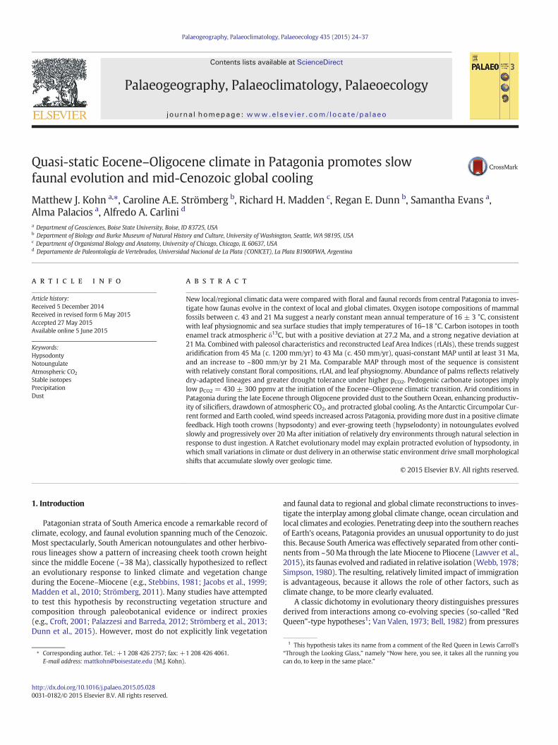
Fig. 1. Locationmap in South America of Gran Barranca (our primary study area), and sec-ondary locations at Scarritt Pocket (SP) and Cañadon Vaca (CV); F=macrofloral localities(Rio Turbio: 51.5°S, 37–45 Ma; Ñirihuau: 41.3°S, 23–28.5 and 19–23 Ma; Las Aguilas:33.3°S, 23–26Ma;Goterones: 33.9°S, ~23Ma; Los Litres: 33.3°S, 21–23Ma). Drake Passageand the Antarctic Circumpolar Current (ACC) separate South America physically andoceanographically from Antarctica. The prevailing westerlies blow across (semiarid)Patagonia towards the Southern Oceans.

25M.J. Kohn et al. / Palaeogeography, Palaeoclimatology, Palaeoecology 435 (2015) 24–37

derived from changes to the environment (e.g. climate and tectonics;so-called “Court Jester”-type hypotheses; Barnosky, 2001). The RedQueen has recently been demoted as being of limited use to explainadaptation or extinction, based on both theoretical and empiricalconsiderations (Vermeij and Roopnarine, 2013), and many deep-timestudies in both North and South America point to climate as a majordriver of evolution, in support of Court Jester hypotheses (Barnosky,2001; Barnosky et al., 2003; Figueirido et al., 2012; Woodburne et al.,2014). In contrast, other comparative work fails to show any relationbetween environmental alteration and faunal change (Prothero, 1999,2004; Alroy et al., 2000); thus the importance of the Court Jester formajor evolutionary trends in faunas remains uncertain.

A major shortcoming of virtually all analyses performed so far is theinappropriate spatial scales of the climate data compared to thebiotic records, with, for example, regional to continent-wide faunal in-formation assessed against global climate data (e.g., Alroy et al., 2000;Figueirido et al., 2012). Considering the mounting evidence that thenature and timing of faunal and floral changes varied from region to re-gion during the Cenozoic (e.g., Leopold and Denton, 1987; Strömberg,2005, 2011; Edwards et al., 2010; Finarelli and Badgley, 2010;Woodburne, 2010), region-by-region analysis seems necessary to dis-cern biologically meaningful patterns.

In this study,we sought to improve upon previouswork by rigorous-ly evaluating links between abiotic change and biotic responses insouthern South America during the Cenozoic (~43 to ~20 Ma), andusing the results to assess the strength of the Court Jester. To do so,we combined new stable isotope data with recent and emerging floraland faunal data from a single, confined region in Patagonia, andanalyzed these records in the context of global climate change. Specifi-cally, we address the following questions:

1) What was the environment like in central Patagonia in terms ofphysical climate variables and vegetation structure and composi-tion? How did these change through time?

2) How did global climate change, as represented by the deep marinerecord, impact local climates? Did abrupt climate shifts, such as theEocene–Oligocene transition, cause abrupt changes to ecosystemsand faunas also in Patagonia? Is there any evidence for localconditions causing feedbacks to global climate?

3) Did climate change impact faunal evolution and if so, what was thetiming and rate of that change in relation to climate? In particular,we wish to evaluate whether faunas rapidly (e.g. b1 Ma) adaptedtooth morphology to a particular climate and ecological condition,or whether they exhibit significantly delayed response suggestingan evolutionary lag or weak selection (Strömberg, 2006).

2. Background

2.1. Geology

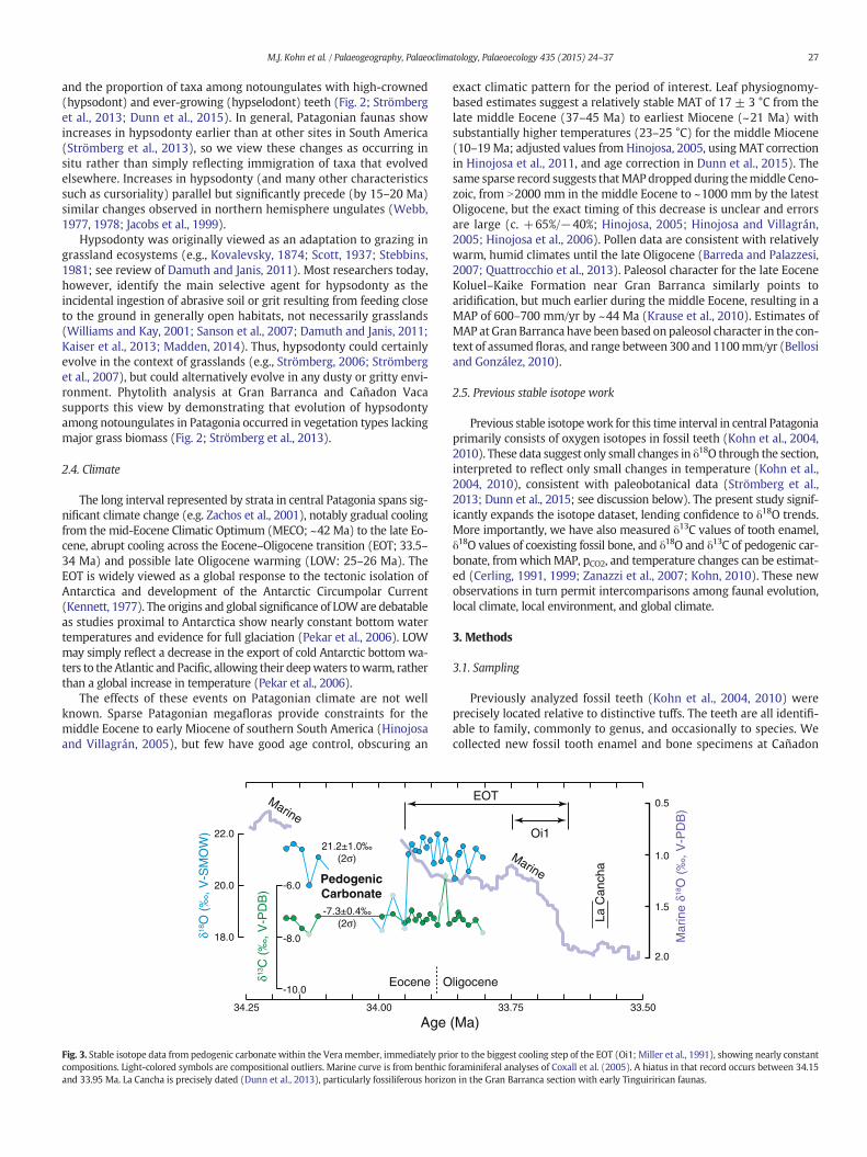
In central Patagonia, a c. 300 meter-thick sequence of fine-grainedtuffaceous sediments – the Sarmiento Formation – hosts numerousfossil localities spanning ~43 to ~19 Ma (Kay et al., 1999; G. Ré et al.,2010; G.H. Ré et al., 2010; Dunn et al., 2013). Gran Barranca is themost fossiliferous and famous of these localities and is exposed insouthern Chubut Province, Argentina (Fig. 1). Collections from thisexposure form the basis for nearly all our interpretations. The SarmientoFormation overlies middle Eocene intensely pedogenically modifiedmudstones and tuffaceous sediments of the Koluel–Kaike Formation,and is overlain byMiocenemarine sediments of the Chenque Formation(Bellosi, 2010).

Although barren of fossils, paleosols of the Koluel–Kaike Formationprovide useful constraints on precipitation (Krause et al., 2010). Theage of the Koluel–Kaike Formation is loosely bracketed between~42 Ma (the oldest overlying age from Gran Barranca; G. Ré et al.,2010) and ~47 Ma (youngest detrital zircon ages from underlying

sediments of the Las Flores Formation; see Supplemental file), and weassume an age of ~45 Ma.

Sarmiento Formation sediments consist dominantly of fine-grained,terrestrial, tuffaceous mudstone, siltstone and fine-grained sandstone,variably reworked via fluvial, eolian and pedogenic processes(Spalletti and Mazzoni, 1979). Zircon trace element patterns are mostconsistent with an arc source (M. Kohn and J. Crowley, unpubl. data),presumably from the distal Andean arc rather than the more proximalintracontinental backarc. From lowest to highest, the Sarmiento Forma-tion consists of six members: Gran Barranca, Rosado, Lower PuestoAlmendra, Vera, Upper Puesto Almendra, and Colhue–Huapi (Fig. 2).The sequence at Gran Barranca spans six successive South AmericanLand Mammal Ages (SALMAs; Madden et al., 2010; Fig. 2); fromoldest to youngest these are the Barrancan, Mustersan, Tinguirirican,Deseadan, Colhuehuapian, and Pinturan. The La Cantera level alsopreserves a faunal assemblage intermediate between Tinguirirican andDeseadan SALMAs. Nearby exposures include (in stratigraphic order)the Itaboraian (Las Flores locality), Riochican (Koluel–Kaike Formation),and Vacan (Cañadon Vaca) SALMAs (e.g., see Woodburne et al., 2014).We generally refer our data to SALMAs in the discussion.

Numerous relatively pristine tuffs occur at Gran Barranca, and basaltflows occur within the Upper Puesto Almendra member. Geochronolo-gy of these volcanic rocks combined with magnetostratigraphy definesa detailed chronostratigraphy (G. Ré et al., 2010; G.H. Ré et al., 2010;Dunn et al., 2013) spanning ~42 to ~19 Ma, with the most fossiliferousstrata between ~40 and ~20 Ma. Despite its numerous geologic andpaleontologic qualities, Gran Barranca does contain major depositionalhiatuses (Bellosi, 2010; G. Ré et al., 2010; G.H. Ré et al., 2010), so we

10 m

Rosado

GranBarranca

PuestoAlmendra

Inferior

PuestoAlmendraSuperior

Vera

Colhue-Huapi

Sar

mie

nto

For

mat

ion

stra

tigra

phy

at G

ran

Bar

ranc

aMaMember SALMA

Tinguirirican

Barrancan

Mustersan

Colhuehuapian

Deseadan

La Cantera

Pinturan18

19

20

21

22

23

24

25

26

27

28

29

30

31

32

33

34

35

36

37

38

39

40

41

42

43

EOT

LOW LOW

Mi1Mi1

Zingiberales

0 100%

Relative abundance of diagnostic phytoliths

Palm

Other “forest”indicators

Closed-habitatgrass

Pooideae

PACMAD

Phytolith classes

EOT

Oi1

MECOMECOCañadon

Vaca

ScarrittPocket

Phy

tolit

h S

ampl

es

IsotopeSamples Notoungulate Hypsodonty Marine Isotopes

Phytolith abundanceSamplesStratigraphy

Mio

cene

Olig

ocen

eE

ocen

e

Dry Wet0.0 1.0 2.0 3.0 4.0

Leaf Area Index

Archaeophyluspatrius

Hyp

sodo

nty

Leaf

Are

aIn

dex

Notopithecusadapinus

Eopachyrucospliciferus

0% 100%

1.02.03.0Foram. δ18O

A CB D E

Fig. 2. Published records and sampling levels relevant to this study. (A) Stratigraphy (Dunn et al., 2013). (B) Sampling levels for isotopes. (C) Phytoliths (Strömberg et al., 2013).(D) Reconstructed Leaf Area Index (rLAI) and proportions of hypsodont plus hypselodont notoungulates (Dunn et al., 2015). Age errors (2σ) shown by vertical bars; some are one-sided because chronologic control provides a maximum bound. Where not shown, errors are smaller than symbols; error bars for hypsodonty are bootstrapped 95% confidence intervals.(E) Benthic foraminiferal isotope record (Zachos et al., 2001). MECO= middle Eocene climatic optimum; EOT = Eocene–Oligocene transition; LOW= late Oligocene warming; Mi1 =early Miocene glaciation.

26 M.J. Kohn et al. / Palaeogeography, Palaeoclimatology, Palaeoecology 435 (2015) 24–37

included fossils of different ages from two nearby localities. Fossils frombasal Sarmiento Formation at Cañadon Vaca (Fig. 1) define the VacanSALMA (Cifelli, 1985; ~43 Ma; Fig. 2), and fossils from Scarritt Pocket(Fig. 1) are from the early Deseadan (27.2 Ma; Vucetich et al., 2014;Supplemental file; Fig. 2). These localities are sufficiently close to GranBarranca that we do not expect significant differences in climate; forexample, modern climatic conditions are indistinguishable.

2.2. Floras

Although plant macrofossils are spectacularly well preserved prior tothe middle Eocene in southern South America (e.g. see Wilf et al., 2013),occurrences are temporally sporadic from the late Eocene through Mio-cene (Hinojosa and Villagrán, 2005). Instead phytoliths (microscopic sili-ca particles formed inside living plants) provide amore continuous recordof floras for the post-middle Eocene (Strömberg et al., 2013; Fig. 2). Thesemicrofossils show that grasses were remarkably sparse between 43 and18.5 Ma, especially during the latest Eocene to middle Oligocene, and in-stead palms, conifers, and “forest” indicators (collectively “dicots,” ferns,conifers, and gingers) dominate. Grass abundances were slightly higher

in the mid/late Eocene (up to ~15% of phytolith assemblages) and in-creased in the early Miocene (up to ~25% of phytolith assemblages;Strömberg et al., 2013). These data conclusively rule out the occurrenceof grasslands through the sequence analyzed. However, although phyto-lith and sparse pollen data were originally interpreted as indicating rela-tively closed, forested habitats (Palazzesi and Barreda, 2012; Strömberget al., 2013), new research on phytolith micromorphology (Dunn et al.,2015) implies that Patagonian plant communities experienced highlight levels characteristic of relatively open habitats. In the absence ofabundant grasses, phytolith and pollen types alone do not necessarily in-dicate habitat openness, and habitats could have ranged from closed torelatively open.

2.3. Faunas

The Sarmiento Formation preserves a rich record of faunas andfaunal evolution. Of special relevance to this study, between ~40 and~20 Ma increases are observed in both mean tooth crown height(hypsodonty or the ratio of tooth crown height to anterior–posteriorlength, here determined on relatively unwornM1molars)within clades

27M.J. Kohn et al. / Palaeogeography, Palaeoclimatology, Palaeoecology 435 (2015) 24–37

and the proportion of taxa among notoungulates with high-crowned(hypsodont) and ever-growing (hypselodont) teeth (Fig. 2; Strömberget al., 2013; Dunn et al., 2015). In general, Patagonian faunas showincreases in hypsodonty earlier than at other sites in South America(Strömberg et al., 2013), so we view these changes as occurring insitu rather than simply reflecting immigration of taxa that evolvedelsewhere. Increases in hypsodonty (and many other characteristicssuch as cursoriality) parallel but significantly precede (by 15–20 Ma)similar changes observed in northern hemisphere ungulates (Webb,1977, 1978; Jacobs et al., 1999).

Hypsodonty was originally viewed as an adaptation to grazing ingrassland ecosystems (e.g., Kovalevsky, 1874; Scott, 1937; Stebbins,1981; see review of Damuth and Janis, 2011). Most researchers today,however, identify the main selective agent for hypsodonty as theincidental ingestion of abrasive soil or grit resulting from feeding closeto the ground in generally open habitats, not necessarily grasslands(Williams and Kay, 2001; Sanson et al., 2007; Damuth and Janis, 2011;Kaiser et al., 2013; Madden, 2014). Thus, hypsodonty could certainlyevolve in the context of grasslands (e.g., Strömberg, 2006; Strömberget al., 2007), but could alternatively evolve in any dusty or gritty envi-ronment. Phytolith analysis at Gran Barranca and Cañadon Vacasupports this view by demonstrating that evolution of hypsodontyamong notoungulates in Patagonia occurred in vegetation types lackingmajor grass biomass (Fig. 2; Strömberg et al., 2013).

2.4. Climate

The long interval represented by strata in central Patagonia spans sig-nificant climate change (e.g. Zachos et al., 2001), notably gradual coolingfrom the mid-Eocene Climatic Optimum (MECO; ~42 Ma) to the late Eo-cene, abrupt cooling across the Eocene–Oligocene transition (EOT; 33.5–34 Ma) and possible late Oligocene warming (LOW: 25–26 Ma). TheEOT is widely viewed as a global response to the tectonic isolation ofAntarctica and development of the Antarctic Circumpolar Current(Kennett, 1977). The origins and global significance of LOWare debatableas studies proximal to Antarctica show nearly constant bottom watertemperatures and evidence for full glaciation (Pekar et al., 2006). LOWmay simply reflect a decrease in the export of cold Antarctic bottom wa-ters to the Atlantic and Pacific, allowing their deepwaters towarm, ratherthan a global increase in temperature (Pekar et al., 2006).

The effects of these events on Patagonian climate are not wellknown. Sparse Patagonian megafloras provide constraints for themiddle Eocene to early Miocene of southern South America (Hinojosaand Villagrán, 2005), but few have good age control, obscuring an

Age

δ18O

(‰

, V-S

MO

W)

34.25

22.0

20.0

18.0

34.00

-7.3±0.4‰(2σ)

Marine

21.2±1.0‰(2σ)

δ13C

(‰

, V-P

DB

) -6.0

-10.0

-8.0

Eocene O

PedogenicCarbonate

Fig. 3. Stable isotope data from pedogenic carbonate within the Vera member, immediately pricompositions. Light-colored symbols are compositional outliers. Marine curve is from benthic fand 33.95 Ma. La Cancha is precisely dated (Dunn et al., 2013), particularly fossiliferous horizo

exact climatic pattern for the period of interest. Leaf physiognomy-based estimates suggest a relatively stable MAT of 17 ± 3 °C from thelate middle Eocene (37–45 Ma) to earliest Miocene (~21 Ma) withsubstantially higher temperatures (23–25 °C) for the middle Miocene(10–19 Ma; adjusted values from Hinojosa, 2005, usingMAT correctionin Hinojosa et al., 2011, and age correction in Dunn et al., 2015). Thesame sparse record suggests thatMAPdropped during themiddle Ceno-zoic, from N2000 mm in the middle Eocene to ~1000 mm by the latestOligocene, but the exact timing of this decrease is unclear and errorsare large (c. +65%/−40%; Hinojosa, 2005; Hinojosa and Villagrán,2005; Hinojosa et al., 2006). Pollen data are consistent with relativelywarm, humid climates until the late Oligocene (Barreda and Palazzesi,2007; Quattrocchio et al., 2013). Paleosol character for the late EoceneKoluel–Kaike Formation near Gran Barranca similarly points toaridification, but much earlier during the middle Eocene, resulting in aMAP of 600–700 mm/yr by ~44 Ma (Krause et al., 2010). Estimates ofMAP at Gran Barranca have been based on paleosol character in the con-text of assumedfloras, and range between 300 and 1100mm/yr (Bellosiand González, 2010).

2.5. Previous stable isotope work

Previous stable isotopework for this time interval in central Patagoniaprimarily consists of oxygen isotopes in fossil teeth (Kohn et al., 2004,2010). These data suggest only small changes in δ18O through the section,interpreted to reflect only small changes in temperature (Kohn et al.,2004, 2010), consistent with paleobotanical data (Strömberg et al.,2013; Dunn et al., 2015; see discussion below). The present study signif-icantly expands the isotope dataset, lending confidence to δ18O trends.More importantly, we have also measured δ13C values of tooth enamel,δ18O values of coexisting fossil bone, and δ18O and δ13C of pedogenic car-bonate, fromwhichMAP, pCO2, and temperature changes can be estimat-ed (Cerling, 1991, 1999; Zanazzi et al., 2007; Kohn, 2010). These newobservations in turn permit intercomparisons among faunal evolution,local climate, local environment, and global climate.

3. Methods

3.1. Sampling

Previously analyzed fossil teeth (Kohn et al., 2004, 2010) wereprecisely located relative to distinctive tuffs. The teeth are all identifi-able to family, commonly to genus, and occasionally to species. Wecollected new fossil tooth enamel and bone specimens at Cañadon

(Ma)

Mar

ine

δ18O

(‰

, V-P

DB

)

0.5

1.0

1.5

2.0

Marine

33.75 33.50

EOT

ligocene

Oi1

La C

anch

a

or to the biggest cooling step of the EOT (Oi1; Miller et al., 1991), showing nearly constantoraminiferal analyses of Coxall et al. (2005). A hiatus in that record occurs between 34.15n in the Gran Barranca section with early Tinguirirican faunas.

28 M.J. Kohn et al. / Palaeogeography, Palaeoclimatology, Palaeoecology 435 (2015) 24–37

Vaca and Gran Barranca mostly from float, prospecting along ridge axesrather than ridge bases or flat areas to minimize downward drift andtime-averaging of fossils. A similar approach (Zanazzi et al., 2009)proved successful in delineating abrupt isotope shifts elsewhere(Zanazzi et al., 2007; Zanazzi and Kohn, 2008). We also collectedpedogenic carbonate nodules through a subsection of the lower Veramember near the Eocene–Oligocene boundary. All specimens werelocated to the nearest 0.1–0.25 m using a Jacobs staff relative to distinc-tive tuffs, which were located within the overall chronostratigraphicframework of Dunn et al. (2013). Note that because of slight variationsin thickness along different transects, our meter levels do not alwaysline up precisely with Dunn et al.'s, but key chronologic horizons areidentical. Ultimately we average many of our data into time slices, sothese minor differences are unimportant.

Tooth enamel fragments were also collected from Cañadon Vacafrom a fossiliferous tuff, geographically isolated from the strati-graphically coherent section. Attempts to separate and date zirconsfrom the tuff were unsuccessful, so we simply assign an average age of~43 Ma to all specimens; this age is intermediate between the VRStuff at Gran Barranca (41.7 Ma; G. Ré et al., 2010), which strati-graphically overlies the Vacan, and the assumed age of the Koluel–Kaike Formation (~45 Ma). Teeth from Scarritt Pocket were obtainedfrom past collections housed at the Museo de la Plata. Fossils and tuffwere collected from a single horizon, so we assign a single age of27.2 ± 0.5 Ma (Vucetich et al., 2014).

Few of the new enamel fragments could be identified to genus orspecies, but microstructural characteristics combined with previousstudies of faunashelp delineate likely families. For example, thick enam-el (≥2 mm thickness) with tiny transverse ridges on occlusal surfaces ischaracteristic of astrapotheres, whereas the occurrence of perikymata(transverse ridges on outer tooth surfaces) is restricted to toxodontids,and enamel from large brachydont to mesodont teeth is probablyderived from leontiniids or isotemnids (two extremely common fami-lies). These distinctions facilitate comparison of isotope compositionsamong different families.

For each tooth enamel fragment, we subsampled a thin sliver alongits growth axis, favoring longer fragments where possible, andpowdered the entire sliver for isotope compositions. This approachaverages isotope zoning, but previous studies have explored zoningfor many levels (Kohn et al., 2004, 2010), and variation among numer-ous different specimens provides an alternate measure of isotopevariability for a particular time slice. For comparison equivalency, weaverage isotope compositions of each serially-sampled tooth fromprevious studies to a single composition. Isotope composition of bonesare commonly quite scattered (e.g. Zanazzi et al., 2007, 2009), so foreach levelwe powdered small fragments of individual bones, pretreatedseparately, then mixed equal amounts (1 mg) into a composite foranalysis. Strictly speaking, bone compositions must post-date enamelcompositions slightly because of the time needed to diageneticallyalter the bone (c. a few tens of ka; see Kohn and Law, 2006). Such asmall time difference is not resolvable in our sampling or dataset. Weattempted to sample 5 bone specimens per level, but several levelswere bone-poor, so composites ranged from 1 to 5 individual bone frag-ments, on average 4. For teeth from Scarritt Pocket, we cut longitudinalslivers on site at Museo de la Plata using a small rock saw, mountedslivers on glass slides using acetone-soluble cement, and subsampledevery ~1–2 mm along the length of the sliver using a slow-speed saw.Individual subsamples were then powdered for analysis.

Pedogenic carbonate nodules were prepared and analyzed for stablecarbon and oxygen isotopes at the Boise State Stable Isotope Laboratory.Nodules were collected with an ~0.2 m spacing from ~33 to ~44 mabove the base of the Vera (34.2 to 33.8 Ma), with a gap between ~35and ~38 m (34.1 to 34.0 Ma; Fig. 3). These levels underlie the preciselydated, fossiliferous La Cancha level (c. 50 m above the member base;33.58 Ma; Dunn et al., 2013), and fall within the earliest stage of theEOT immediately prior to the main Oi1 phase (Fig. 3). Carbonate

nodules were not found elsewhere along our transect and are randomlydistributed, which we interpret to reflect continuous aggradation of su-perposed Bk horizons (Bk refers to the level of carbonate accumulationin a soil; Soil Survey Staff, 2010). Texturally analogous nodules from theVera are illustrated in (Bellosi and González, 2010; their Fig. 20.2-9; seeSupplemental file).

3.2. Isotope analysis

Fossil tooth, bone, and reference NIST120c powders were identicallypretreated using themethod of Koch et al. (1997) and analyzed for δ13Cand δ18O values of structural carbonate (Table 1) using an automatedextraction system (Gasbench II) attached to a ThermoFisher Delta V-Plus mass spectrometer housed in the Stable Isotope Laboratory, De-partment of Geosciences, Boise State University. Pedogenic carbonatenodules consist solely of micritic calcite (no sparry calcite was found),so a small portion was powdered and analyzed using the same analyti-cal system. Raw datawere standardized against NIST18 and NIST19 car-bonates, whose analytical reproducibilities for both C- and O-isotopeswere ±0.2–0.3‰ (±2σ). Biogenic phosphate δ18O values exhibitsmall but systematic session-to-session variations in absolute values.Consequently, we made further small corrections based on concurrentanalysis of NIST120c (a phosphorite with broadly similar bioapatitechemistry as fossil teeth and bones), assuming a composition of28.50‰ (V-SMOW) based on an ~10 year average of analyses collectedin our laboratory. Average values for NIST120c δ18O range from 28.2 to28.8‰ (V-SMOW). Carbon isotope values require no additional correctionand for NIST120c average−6.55‰ (V-PDB). Reproducibility on NIST120cwas approximately ±0.25‰ for δ13C and ±0.6‰ for δ18O (2σ).

3.3. Temperature calculations from fossil bones and teeth

The fractionation of oxygen isotopes between fossil bone and enam-el can potentially elucidate changes in air (soil) temperature (Zanazziet al., 2007) because bone is diagenetically altered at ambient soil tem-peratures (Kohn and Law, 2006) whereas enamel retains its originalcomposition imparted at mammal body temperature (i.e. 37 °C). Theapproach of Zanazzi et al. (2007) and modern calibrations for Bovinaeand Equidae (Kohn and Dettman, 2007; Kohn and Fremd, 2007) yieldthe following equation:

T �Cð Þ ¼ 18030

1000 ln1þ δ18Obone−2:2

� �=1000

1þ 1:15 � δ18Oenamel−36:3� �

=1000

0@

1Aþ 32:42

−273:15 ð1Þ

where δ18O of bone and enamel is expressed on the V-SMOW scale.

3.4. MAP calculations

Carbon isotope values of C3 plants and their consumers track theδ13C of atmospheric CO2, but also correlate negatively with MAP(e.g., Stewart et al., 1995). These dependencies were calibrated usingmodern data to permit calculation of MAP (Kohn, 2010):

MAP ¼ 10˄ Δ13C−2:01þ 0:000198 � elev−0:0129 � Abs latð Þ5:88

" #−300 ð2Þ

where elev = elevation in meters, lat = latitude in degrees, and

Δ13C ¼ δ13Catm−δ13Cleaf

1þ δ13Cleaf=1000ð3Þ

where δ13Catm and δ13Cleaf are the carbon isotope compositions ofatmospheric CO2 and vegetation, respectively, as determined fromproxies. The benthic foraminiferal record provides a proxy for δ13Catm

Table 1Summary of mean isotope compositions, δ13C of atmospheric CO2, and calculated MAP.

Time slice δ18Oe ± 2 s.e. δ18Ob ± 2 s.e. δ13Ce ± 2 s.e. δ13Cb ± 2 s.e. δ13Ca MAP ± 2σ T (°C) ± 2 s.e.

Vacan 23.25 ± 0.67 22.06 ± 0.39 −10.65 ± 0.42 −8.44 ± 0.29 −5.85 390 ± 120 19.1 ± 4.1Barrancan 22.39 ± 0.88 22.52 ± 0.33 −11.36 ± 0.48 −9.43 ± 0.22 −5.97 590 ± 180 12.4 ± 4.9Barrancan — anom. 21.85 ± 1.24 n.a. −10.81 ± 0.45 n.a. −5.97 420 ± 130Mustersan 23.07 ± 0.77 22.87 ± 0.49 −11.15 ± 0.56 −8.53 ± 0.32 −6.20 450 ± 170 14.4 ± 4.7Tinguirirican (ave) 23.32 ± 0.54 n.a. −10.54 ± 0.55 n.a. −5.75 400 ± 160Tinguirirican (early) 23.45 ± 0.57 22.61 ± 0.64 −10.74 ± 1.30 −9.74 ± 0.43 n.a. n.a. 17.7 ± 4.3Tinguirirican (late) 23.28 ± 0.69 n.a. −10.43 ± 0.51 n.a. n.a. n.a.La Cantera 23.77 ± 0.65 n.a. −11.27 ± 0.46 n.a. −6.07 530 ± 160Deseadan (early) 23.02 ± 0.78 n.a. −10.22 ± 0.77 n.a. −6.27 200 ± 160Deseadan (late) 21.97 ± 0.27 n.a. −11.55 ± 0.44 n.a. −5.88 700 ± 180Colhuehuapian 23.01 ± 0.28 22.71 ± 0.34 −11.98 ± 0.36 −9.91 ± 0.22 −6.09 800 ± 160 14.8 ± 2.1

Note: Isotope compositions are in permil relative to V-SMOW(δ18O) and V-PDB (δ13C). MAP=mean annual precipitation inmm/yr (rounded to nearest 10mm). Subscripts: e= enamel,b = bone, a = atmospheric CO2. Barrancan — anom. shows the means after removing anomalously low δ13C data from a specific horizon. For Tinguirirican data, ave = all data, early =prior to the EOT, late = after the EOT. Temperature calculations propagate errors in isotope compositions only.

29M.J. Kohn et al. / Palaeogeography, Palaeoclimatology, Palaeoecology 435 (2015) 24–37

(Tipple et al., 2010). Although we have no direct measure of plant com-positions, tooth enamel in modern perissodactyls (horses, rhinos, andtapirs) exhibits a constant, ~14‰ offset relative to diet (Cerling andHarris, 1999). Perissodactyls are hindgut fermenters, retaining theplesiomorphic digestive physiology. Recent fossil protein sequenceanalysis linking South American (meridi)ungulates most closely tocrown Perissodactyla (Buckley, 2015; Welker et al., 2015) and thestrong similarities in cranio-dental morphology between perissodactylsand notoungulates (Fletcher et al., 2010; Cassini et al., 2012), suggestthat notoungulates were also hindgut fermenters and justifies use of asimilar offset to estimate plant δ13C values and hence MAP (Kohnet al., 2010). That is, δ13Cleaf = δ13Ctooth enamel − 14‰. Note that CAMplants neither form a large biomass component in most ecosystemsnor are consumed in quantity by most herbivores, and that C4 plantswere absent or at least very rare until long after the time period ofinterest (Cerling et al., 1997; Edwards et al., 2010; Strömberg,2011).

Mean annual precipitation was calculated from carbon isotopecompositions of tooth enamel by first subtracting 14‰ to determineδ13Cleaf, then applying Eqs. (2) and (3), basing δ13Catm on Tipple et al.(2010). In principle, MAP above 1700mm/yr may be difficult to quanti-fy because very dense forests have anomalously low δ13C values (−32to −37‰ in modern ecosystems; see Kohn, 2010). Inferred δ13Cleaf

values in this study are well above any likely closed forest values,however, so no additional correction is needed. Random uncertaintiesare propagated based on compositional scatter of the isotope data(standard errors). Systematic errors in the MAP calibration areapproximately ±50% (2σ) of the absolute value (Kohn and McKay,2012). We made no correction of δ13C for pCO2 because corrections(Schubert and Jahren, 2012) applied to published tooth enamel dataworldwide imply negative MAP for the Oligocene, implausibly lowMAP (≤350 mm/yr) for demonstrably wet periods of the Paleocene,Eocene and Miocene, and implausibly high MAP (≥2000 mm/yr) forthe relatively dry Pleistocene (Kohn, 2014). Similarly, many tree ringisotope studies covering the last century do not independently resolvea pCO2 effect on isotope discrimination (e.g., Saurer et al., 2004). Otherestimates of MAP in South America were taken from studies of leafphysiognomy for sites 300–700 km NW of the study area (Fig. 1;Hinojosa, 2005; Hinojosa and Villagrán, 2005; Hinojosa et al., 2011)and from paleosols of the Koluel–Kaike Formation (Krause et al.,2010) and the Sarmiento Formation at Gran Barranca (Bellosi andGonzález, 2010). The latter estimates, however, may be biased by localsediment accumulation rates (see further discussion below).

3.5. pCO2 calculations

The δ13C of pedogenic carbonate can be used to estimate pCO2

provided the following compositional and concentration parameters

are constrained (Cerling, 1991, 1999): the concentration of soil CO2

[S(z)] and values for δ13Cs, δ13CΦ and δ13Ca, where subscripts s, Φ, anda refer to soil CO2, respired CO2 (commonly taken as soil organic carbonδ13C), and air CO2:

pCO2¼ S zð Þ δ13Cs−1:0044 � δ13CΦ−4:4

δ13Ca−δ13Cs

" #: ð4Þ

We estimated δ13Cs (soil CO2) from measured mean pedogeniccalcite as corrected for formation temperature according to experimen-tal calibrations (Romanek et al., 1992):

1000δ13CCaCO3 þ 1000

δ13CCO2 þ 1000

!−1

" #¼ 11:98−0:12 � T �Cð Þ: ð5Þ

Because organic carbon contents of these sediments are extremelylow, our preferred value for δ13CΦ is based on mean δ13C values oftooth enamel carbonate (−10.5 ± 0.5‰; Kohn et al., 2010, thisstudy), corrected downward by 14‰ for leaf-enamel fractionation(Cerling and Harris, 1999) and corrected upward by 2 ± 1‰ for thedifference between bulk leaf vs. soil organic matter in modern soils(Bowling et al., 2008). The value for δ13Ca is again based on benthicforaminiferal records (Tipple et al., 2010). For S(z), recentwork suggestsa typical value during pedogenic carbonate precipitation of 2500 ±1000 ppm (Breecker et al., 2010). A regression of S(z) vs. MAP (Cottonand Sheldon, 2012) implies a similar S(z) of ~2300 ppm, using MAPvalues determined from isotope data (see below) and paleosolcharacter in the Vera Member (Bellosi and González, 2010; 300–650 mm/yr).

4. Results

Isotope compositions of pedogenic carbonate nodules are remark-ably homogeneous through the c. 400 ka section analyzed (Fig. 3).Omitting a few outliers at low δ18O and high δ13C, which mayreflect nodules that formed closer to paleosurfaces, average valuesare δ13C = −7.3 ± 0.4‰ (V-PDB; 2σ) and δ18O = 21.2 ± 1.0‰(V-SMOW; 2σ). These are some of the first isotope data from definitivepedogenic carbonates collected proximal to the EOT, and δ13C values arewell within the range reported globally for Eocene and Oligocenepaleosols (Ekart et al., 1999; Sheldon and Tabor, 2009; Sheldon et al.,2012; Srivastava et al., 2013). In combination with published toothenamel δ18O and δ13C values, pCO2 and paleotemperature may beestimated.

Compositions for enamel and bone scatter by ~±2‰ for both carbonand oxygen for each time slice (Fig. 4A–B). Such scatter is expectedmainly because of intra-tooth zoning that encodes seasonal isotope

Age

(M

a)

Barrancan

Vacan

early Deseadan

late Deseadan

Colhuehuapian

Pinturan

Tinguirirican

La Cantera

Mustersan

45

40

35

30

25

20

15Enamel Bone Enamel Bone

δ13C (‰, V-PDB)

Age

(M

a)

Foram. δ18O

EOT

LOW

Mi1 Mi1

-16.0 -6.0-8.0-10.0-12.0-14.0 27.017.0 19.0 21.0 23.0 25.045

40

35

30

25

20

15

δ18O (‰, V-SMOW)

Atm δ13C-5‰

wetter drier

Bone averageEnamel average Bone averageEnamel average

A B

C D

3.0 1.0

Foram. δ18O

EOT

MECO MECO

LOW

3.0 1.0

Barrancan

Vacan

early Deseadan

late Deseadan

Colhuehuapian

Pinturan

Tinguirirican

La Cantera

Mustersan

Fig. 4. Stable isotope data from fossil tooth enamel and bone. (A–B) Raw data for individual tooth enamel fragments and bone composites for carbon isotopes (A) and oxygen isotopes (B),illustrating broadly comparable data ranges through time. Small ellipse in A emphasizes cluster of anomalously low δ13C values during a specific short interval (39.2 to 39.0 Ma). (C–D)Time-slice averages with reference global atmospheric (Tipple et al., 2010) and deep marine curves (Zachos et al., 2001). Light blue symbols in Barrancan show the effect of removingcluster of anomalous δ13C values frommean; light blue symbols in Tinguirirican distinguish the compositions immediately pre- andpost-EOT. Error bars are±2 s.e. Relative to atmospher-ic δ13C values minus 5‰, tooth enamel δ13C values are generally comparable or slightly higher until 27.2 Ma then significantly lower. Enamel δ18O values are indistinguishable throughtime except at ~23 Ma. Bone δ18O values are not significantly different from enamel except for the Vacan. (For interpretation of the references to color in this figure legend, the readeris referred to the web version of this article.)

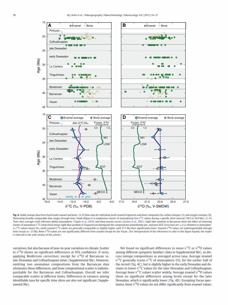
30 M.J. Kohn et al. / Palaeogeography, Palaeoclimatology, Palaeoecology 435 (2015) 24–37

variations, but also because of year-to-year variations in climate. Scatterin δ18O shows no significant differences at 95% confidence (F-tests,applying Bonferroni correction) except for δ18O of Barrancan vs.late Deseadan and Colhuehuapian times (Supplemental file). However,omitting two anomalous compositions from the Barrancan dataeliminates these differences, and bone compositional scatter is indistin-guishable for the Barrancan and Colhuehuapian. Overall we infercomparable scatter at different times. Differences in variance amongidentifiable taxa for specific time slices are also not significant (Supple-mental file).

We found no significant differences in mean δ13C or δ18O valuesamong different sympatric families (data in Supplemental file), so dis-cuss isotope compositions as averaged across taxa. Average enamelδ13C generally tracks δ13C of atmospheric CO2 for the earlier half ofthe record (Fig. 4C), but is slightly higher in the early Deseadan and de-viates to lower δ13C values for the later Deseadan and Colhuehuapian.Average bone δ13C values scatter widely. Average enamel δ18O valuesshow no significant differences among levels except for the laterDeseadan, which is significantly lower (Fig. 4D). Excepting Vacan spec-imens, bone δ18O values do not differ significantly from enamel values.

31M.J. Kohn et al. / Palaeogeography, Palaeoclimatology, Palaeoecology 435 (2015) 24–37

5. Discussion

5.1. Oxygen isotopes and Patagonian paleoclimate

Our expanded dataset corroborates previous studies (Kohn et al.,2004, 2010) that showed no significant change to δ18O values throughthe section, except during Deseadan time. Note that Kohn et al. (2010)assumed an age for the Deseadan fossils at Gran Barranca of ~27 Ma,but the fossils occur along a disconformity whose age is bracketedbetween 26.3 ± 0.3 and ≤23.1 Ma (Ré et al., 2010a; Dunn et al., 2013).Regardless, these fossils postdate Deseadan faunas at Scarritt Pocket(27.2 Ma; Vucetich et al., 2014). The climatic implications of constantδ18O values must be considered in the context of changes to globalocean δ18O attending changes in ice volume. Specifically, growth ofthe Antarctic ice sheet during the EOT should have raised ocean andprecipitation δ18O values by ~1‰ (Coxall et al., 2005). One possiblereason this increase is not observed is that decreasing temperaturenormally decreases precipitation δ18O values, with a coefficient of~0.35‰/°C atmid- to high latitudes (see Kohn et al., 2002). Correlationsbetween biogenic phosphate and local water δ18O (e.g. Kohn, 1996;Kohn and Cerling, 2002) imply an ~0.3‰ decrease in enamel δ18O perdegree of cooling. Thus, constant δ18O values across the EOT in thecontext of a 1‰ rise in the global meteoric system could indicate atemperature decrease of c. 3–4 °C (1‰ ÷ 0.3‰/°C; Kohn et al., 2010).Alternatively, small changes to moisture sources at constant tempera-ture could have offset the global increase in water δ18O. For example,changes in the position and intensity of the westerlies have beendocumented during the Quaternary, affecting plant communities andhydrology (e.g., Moreno et al., 2012). Similar changes might have influ-enced isotope compositions to offset the global shift independent oftemperature. Constant δ18O values subsequent to the EOT are consistentwith quasi-constant temperatures and ice volume through the Oligo-cene and (arguably) the earlyMiocene, supporting previous suggestionsthat late Oligocene warming was not manifest at high southernlatitudes (Pekar et al., 2006). Even if late Oligocenewarmingwas a glob-al phenomenon, high ice volume in Antarctica (i.e. quasi-constant globalocean compositions; Pekar et al., 2006) may indicate that temperaturedid not change significantly in central Patagonia. A constant tempera-ture is consistent with indistinguishable MAT estimates for late Eocenethrough early Miocene floras in southern South America (Hinojosa andVillagrán, 2005; Hinojosa et al., 2006, 2011; see discussion below).

The ~1.1‰ dip in δ18O values for late Deseadan fossils at GranBarranca might reflect deep glaciation associated with Mi1 at 23 Ma(Miller et al., 1991). Because the disconformity from which the fossilsderive spans at least 3 Ma, we cannot definitively pin the isotopes tothis event. But possibly abrupt cooling catalyzed erosion of underlyingsediments and accumulation of teeth. If so, the isotope shift would beconsistent with brief cooling of at least 4 °C (1.1‰ ÷ 0.3‰/°C).

Application of Eq. (1) (above) to bone and enamel compositionsthrough the sequence (Fig. 4) implies relatively constant alterationtemperatures of 16 ± 3 (2 s.e.) °C. Unfortunately we lack bone fromafter the EOT to independently test interpretations of temperaturechanges derived from oxygen isotope trends alone. Calculated temper-atures are lower than body temperature because, although isotopecompositions are comparable for bone and enamel, body water δ18Ofor large, water-dependent herbivores is typically at least 5‰ higherthan local water (e.g. Kohn and Cerling, 2002). That is, enamel andbone δ18O values may be similar, but the water δ18O values withwhich the bioapatite equilibrated differed considerably. We assumethat bone does not preserve original biogenic compositions because itsδ13C values are substantially different from enamel in many levels. Thecalculated alteration temperature is higher than modern day MAT(11.0 °C for Sarmiento, Argentina), and overlaps temperatures estimat-ed from marine and floral data of the mid-Cenozoic. Models of oceancirculation anchored to measurements of temperature from bivalveshells spanning 34 to 45 Ma imply essentially constant MAT = 15–

17 °C for coastal South America at the latitude of Gran Barranca(Douglas et al., 2014). Insofar as temperature in Patagonia is stronglybuffered by proximity to the ocean, Douglas et al.'s observations andour new isotope data imply that temperatures in the region decreasedrelatively little between the Eocene and early Miocene. Floral analysissimilarly implies statistically indistinguishable MAT values of 17 ±3 °C from the Eocene through early Miocene (Hinojosa and Villagrán,2005; Hinojosa et al., 2006), although later calculations using leafphysiognomy methods calibrated to South American floras produceMAT values that are ~1.5 °C lower (Hinojosa et al., 2011). A value forMAT of 14–18 °C fits observations for all data except the late Deseadan.

Variation in δ18O is commonly taken to reflect changes in local waterδ18O, which in turn responds to temperature. For example, δ18O zoningin teeth closely tracks seasonal meteoric water composition, whichcorrelates with seasonal temperature (e.g., Fricke and O'Neil, 1996;Kohn, 1996). In general, our sampling protocol did not resolve sufficientfine-scale detail to warrant close comparisons among levels. However,the ±2‰ range divided by the temperature coefficient for seasonalisotope variations in large herbivores at mid-latitudes (0.3‰/°C;Zanazzi et al., 2007) implies a minimum estimate of the mean annualrange of temperature (MART) of ~13 °C, identical to estimates ofMART derived from Eocene through early Miocene floras of southernSouth America (13–14 °C; Hinojosa and Villagrán, 2005). In combina-tion with a MAT of 16 °C, this range implies a warm-month meantemperature (WMMT) of 23 °C. The range of variation does not appearto differ significantly among levels, implying similar MART through thesequence.

The δ18O of pedogenic calcite can also beused to infer temperature, ifthe δ18O of soil water is known independently. This temperature isexpected to reflect WMMT because pedogenic carbonate forms prefer-entially during the dry (usually warmest) season (Breecker et al.,2009). Tooth enamel δ18O correlates closely with local water δ18O (e.g.see review of Kohn and Cerling, 2002), so we used δ18O values fortooth enamel from the Vera Member (Kohn et al., 2010; this study)and global correlations for water-dependent ungulates (Kohn andCerling, 2002; Kohn and Dettman, 2007; Kohn and Fremd, 2007) to de-rive local water δ18O. Because we infer a plesiomorphic hindgutdigestive physiology for meridiungulates (see above) we reasonablyassume that they were water dependent like all perissodactyls today(McNab, 2002). These data imply a local water composition of~−8.5 ± 1.0‰ (V-SMOW), with the largest uncertainty resultingfrom scatter in modern correlations. Together with a mean pedogeniccalcite value of 21.3±0.2‰ (V-SMOW, 2 s.e.), the experimental calibra-tion of Kim and O'Neil (1997) implies a precipitation temperature of18 ± 6 °C. This temperature overlaps with but is slightly lower thanWMMT independently estimated above from MAT, MART, and sea-surface temperature (~23 °C). Increasing assumed soil water δ18O by1‰ (e.g., reflectingmodern calibration errors or soil water evaporation)would increase calculatedWMMT by 5 °C and reconcile all temperaturecalculations.

5.2. Pedogenic carbonate and pCO2

For calculating pCO2, we estimated δ13Cs (−16.5‰) from pedogeniccarbonate δ13C (−7.3 ± 0.1‰) assuming carbonate formed at aWMMT temperature of 23 °C. Other parameters include δ13Ca =−6.0‰ (Tipple et al., 2010) and δ13CΦ = −22.5 ± 1‰ based onmean δ13C values of tooth enamel carbonate (−10.5 ± 0.5‰; Kohnet al., 2010; this study) and offsets between bulk leaves and soil organicmatter (Bowling et al., 2008). Taken together, these values implypCO2 = 430 ± 250 ppmv, indistinguishable from estimates from mid-Oligocene paleosols in India (433 and 633 ppmv, uncertainties notreported; Srivastava et al., 2013). Including a temperature error of±5 °C increases total propagated uncertainties to ±300 ppmv (higherWMMT implies higher pCO2). Such a low pCO2 (b750 ppmv) contrastswith marine proxies that typically imply values of 800–1000 ppmv

32 M.J. Kohn et al. / Palaeogeography, Palaeoclimatology, Palaeoecology 435 (2015) 24–37

immediately preceding the EOT (Pearson et al., 2009; Zhang et al.,2013). A drop in pCO2 just before Oi-1, however, as implied by ourdata, is a logical driver of global cooling during the EOT (DeConto andPollard, 2003).

5.3. Carbon isotopes and MAP

Specific MAP estimates from carbon isotopes (Fig. 5A) show noresolvable changes from 43 to 30 Ma, even across the EOT. A meancalculated value of ~450 mm/yr (±200 mm) implies semi-arid condi-tions. Systematic errors would shift all data uniformly, so the constancyof these estimates, which reflects the constant offset between toothenamel and atmospheric δ13C (Fig. 4C), is robust. Note that slightlyhigher apparent MAP values during the Barrancan (c. 600 mm/yr) arecontrolled by low δ13C values during an ~200 ka interval (ellipse inFig. 4A); omitting these data lowers Barrancan MAP to ~400 mm/yr,indistinguishable from the Vacan and Mustersan. During the earlyDeseadan (27.2Ma), MAP appears to drop. However, we have relativelyfew fossils from this locality (Fig. 2B), so although their compositionsare internally consistent, we are cautious in interpreting this timeslice. They certainly do not indicate wetter conditions. MAP at ~23 and~21 Ma shows a distinct rise. Paleofloral estimates of MAP in southernSouth America (Hinojosa, 2005; Hinojosa and Villagrán, 2005) aregenerally higher (average c. 1000 mm/yr), but uncertainties are large(standard errors on the order of 450–1000 mm), and minimumestimates overlap our calculations. A systematic calibration error of200–250 mm/yr for isotope-derived MAP, which is within calibrationuncertainties, would also help reconcile these datasets.

Paleosol estimates of MAP based on soil type and chemistry showgenerally highMAP (up to 1300mm/yr) in the Koluel–Kaike Formation,and a drop towards low MAP values similar to ours at 43 Ma (Krause

0%

Pean

H

MAP (mm/yr)

Age

(M

a)

Barrancan

Vacan

K-K

e. Deseadan

l.. Deseadan

Colhuehuapian

Pinturan

Tinguirirican

La Cantera

Mustersan

045

40

35

30

25

20

15

200 400 600 1200800 1000

A Bδ13C-based

paleosol-based

floral-based

Fig. 5. (A) Estimate of mean annual precipitation (MAP) from tooth enamel δ13C values (this stmacrofloras (green bars; Hinojosa, 2005; Hinojosa and Villagrán, 2005; ages corrected in Dunn(possiblywetter at ~39Ma), and an increase inMAP towards 20Ma. Light symbol for BarrancanKoluel–Kaike Formation. Error bars are propagated 2s.e. in δ13C. (B) Notoungulate hypsodontypercent hypsodont plus hypselodont taxa; blue dots show hypselodont percentages only. Errorwith approximate boundaries of major ecosystems, corroborating relatively dry (open) condit(early Miocene). Red line is a 5-point running average; error bars are 95% confidence intervals.cords. (For interpretation of the references to color in this figure legend, the reader is referred

et al., 2010). Lateritic soils, characteristic of the lower Koluel–KaikeFormation, form only at high MAP (≥1200 mm/yr; e.g. Retallack,2008), strongly suggesting aridification from the (lower) Koluel–Kaiketo the Vacan. In the Sarmiento Formation at Gran Barranca, estimatesof MAP from paleosols (or the inferred vegetation associated withthem; Bellosi and González, 2010) and carbon isotope measurementsoverlap, but suggest that the Barrancan may have been slightly wetterthan times immediately before or after. Younger paleosols also suggestan increase in MAP after ~25 Ma. The higher MAP estimates fromBellosi and González (2010) for the Barrancan, late Deseadan andColhuehuapian, however, correlate with more mature soils and lowersediment accumulation rates (by a factor of 2; Dunn et al., 2013).Paleosol-basedMAP estimatesmay be systematically biased by differentdurations of paleosol development (Zanazzi et al., 2009). Although sed-imentation rate might followMAP (e.g., perhaps sediments accumulatefaster during drier times because delivery rates increase), any factor thataffects sedimentation rate could potentially masquerade as changes toMAP (e.g. perhaps sediments accumulate faster when ash productionis higher). In that respect, indistinguishable floras in the late Barrancanand Mustersan (Fig. 3; Strömberg et al., 2013) may be more consistentwith constant MAP than the decrease suggested by paleosols. Althoughearly aridification and late wetting trends appear robust, the smallvariations between these trends may be less reliable. Overall, we viewthe data as more consistent with relatively constant MAP between 43and at least 31 Ma, possibly as late as 25 Ma.

5.4. The paleoclimatic significance of high MAP floral indicators

The semi-arid conditions inferred from our record might at firstappear at odds with MAP calculations and ecosystem reconstructionsfrom leaf physiognomy and palynofloral and phytolith assemblages

Hyp

selodont

50% 100%

rcent hypsodontd hypselodont

ypso

dont + Hypse

lodo

nt

0.0 1.0 2.0 3.0 4.0

Leaf Area Index

5-ptrunningaverage

Desert/Shrub

Dry Forest/Scrub

BroadleavedForest

C

udy), paleosols (red, yellow symbols; Krause et al., 2010; Bellosi and González, 2010) andet al., 2015), implying aridification between ~48 and ~43 Ma, dry conditions until 25 Mashows the effect of omitting a low δ13C cluster in a specific horizon (ellipse, Fig. 4A). K–K=record for central Patagonia showing the gradual changes through time. Green dots showbars are bootstrapped 95% confidence limits. (C) Leaf area index from Dunn et al. (2015)

ions from the late Barrancan and Mustersan (late Eocene) through middle ColhuehuapianDashed lines temporally correlate MAP estimates with hypsodonty and leaf area index re-to the web version of this article.)

33M.J. Kohn et al. / Palaeogeography, Palaeoclimatology, Palaeoecology 435 (2015) 24–37

from southern South America. The high abundance of palms prior to theearly Miocene and the occurrence of gingers in the middle Eocene, aswell as the generally ‘mixed’ composition of the floras have commonlybeen assumed to reflect high MAP, c. 1000 mm/yr or more (Hinojosa,2005; Hinojosa and Villagrán, 2005; Hinojosa et al., 2006; Barreda andPalazzesi, 2007; Quattrocchio et al., 2013; Strömberg et al., 2013).Several factors qualify inferences from floras, however. First, MAP esti-mates from leaf physiognomy carry large uncertainties – 40 to 65% –and theminimum bounds on MAP overlap our isotope-based estimatesafter accounting for age uncertainties (Fig. 5; Dunn et al., 2015). Second,the leaf physiognomy database has traditionally been heavily skewedtowards northern hemisphere floras. Estimates of MAT show hemi-spheric bias, so temperature estimates now use hemisphere-specificcalibrations (e.g. Hinojosa et al., 2011; Peppe et al., 2011; Kennedyet al., 2014). Similar hemispheric bias might occur for MAP, but is notyet studied. Third, although confined primarily to tropical rainforeststoday (e.g., Couvreur and Baker, 2013), palms contain wider ecologicaltolerance than is commonly recognized. Specifically, many membersof the South American clade Attaleinae, which is represented byPaleocene fossils nearby (Futey et al., 2012), are relatively tolerant ofwater stress and disturbance. Thus, the commonly assumed correspon-dence between palms and high MAP may collapse in this region ofSouth America — quantitative MAP estimates overlap semiarid condi-tions, and the palms that were present may have been relativelyresistant to water stress. These observations do not explain gingers,but perhaps they were restricted to local wet depressions, which canoccur in a variety of settings.

A final consideration is that plants close their stomata under higherpCO2, which dramatically improves water use efficiency (Ehleringer andCerling, 1995; Ainsworth and Rogers, 2007; Ibrahim et al., 2010). For ex-ample, steadily increasing pCO2 has measurably improved water use ef-ficiency across Eurasia during the last century (but without changingisotope discrimination: Saurer et al., 2004). This effect has two implica-tions in the context of higher pCO2 during the Eocene and possibly laterperiods. First, plants such as palms that are now considered to be re-stricted to relative wet ecosystems could have thrived under drier con-ditions such as we propose here (Dunn et al., 2015). Second, becauseplants contribute significantly to atmospheric water vapor, improvedwater use efficiency would have diminished water vapor worldwide,slowing the water cycle and decreasing MAP. Overall, we appreciatethe apparent disparity between our isotope-based estimates of MAPvs. taxonomic floral observations, but suggest that our estimates in theface of other factors are quantitatively correct and, in fact, hint at non-analog ecosystems in Earth's past.

5.5. Did Patagonian dust drive Eocene cooling and the Eocene–OligoceneTransition?

The EOT is generally understood to reflect marine and atmosphericcirculation responses to the opening of marine gateways betweenAntarctica and both South America and Australia (Kennett, 1977), andis associated with an increase in southern ocean productivity, anincrease in terrestrial sediment delivery to the southern ocean, anda decrease in pCO2 (e.g., see Salamy and Zachos, 1999; Coxall andWilson, 2011; Zhang et al., 2013). Here we propose that these environ-mental changeswere all linked through Patagoniandust production as aresult of the semi-arid climate reconstructed from isotopes and otherlines of evidence (see above).

Some of the highest sustained winds on Earth blow across Patagoniabetween 40 and 50° S latitude – the so-called “Roaring 40s” – whichtogether with unusually extensive exposures of highly erodable volca-nic dust deposits help explain why Patagonia is the largest source ofdust to the southern oceans during the Quaternary (Wolff et al., 2006;Li et al., 2008). We suggest that the output of dust from Patagonia hasbeen substantial during at least the last 35 Ma. Progressive isolation ofAntarctica and development of the Antarctic Circumpolar Current

during the Eocene and early Oligocene likely increased wind speedsacross Patagonia (Ladant et al., 2014). If Patagoniawas already relativelydry by the end of the Eocene (Mustersan, Fig. 5; Dunn et al., 2015),increased delivery of dust-sourced Fe, Si and P to southern oceansfrom this already dry and highly erodable environment (sparselyvegetated, tephric soils) would have promoted higher productivity,particularly of silicifiers (Diester-Haass and Zahn, 1996; Salamy andZachos, 1999; Coxall et al., 2005) and decreased CO2, much as increaseddust delivery during the Pleistocene served as a positive feedbackin reducing CO2 and intensifying glaciations (e.g., Martin, 1990;Martinez-Garcia et al., 2011). The drawdown in CO2 from the late Eo-cene to Oligocene (Zhang et al., 2013) served as a positive feedback todrive Antarctic glaciation and thermal isolation, ultimately transformingEarth from greenhouse to icehouse conditions. One notable feature ofEocene–Oligocene climate is the long decline in global temperaturebetween 42 and 34 Ma (i.e. between the MECO and EOT; Zachos et al.,2001; Fig. 2) and in pCO2 between 42 and ~25 Ma (Zhang et al., 2013).If aridification of Patagonia played a key role in this process, then globalclimate responded slowly overall, albeit with a marked step at the EOT.Further studies of mid-Cenozoic dust accumulation in South Atlanticmarine cores would help test this hypothesis.

5.6. Faunal evolution: is the Court Jester a viable hypothesis?

Although Patagonian notoungulates crossed a hypsodonty indexthreshold of 1.0 relatively early (Strömberg et al., 2013), the overallrecord of increasing proportions of hypsodont and hypselodont taxaappears remarkably gradual (Figs. 2B, 5B). Indeed, if hypsodonty wasan adaptation to dry, dusty environments, then it is striking that,although notoungulate hypsodonty did begin increasing soon after theinitiation of semi-arid conditions by the late Eocene, the proportion ofhyposodont + hypselodont taxa did not approach 100% for at leastanother 7 Ma, arguably until 20 Ma. Similarly, hypselodont taxa showa slow increase and do not constitute a majority in faunas even after~20 Ma. The correspondence of reduced MAP, reduced vegetation cover,and increased hypsodonty does make sense— researchers have long rec-ognized that lower MAP correlates with lower plant biomass, increasederosion, and increased sediment concentration in streams (Langbeinand Schumm, 1958). Indeed modern day Patagonia is remarkable for itshigh wind speed and anomalously high rates of dust remobilization anddeposition (Paruelo et al., 1998; Zender et al., 2003). Yet, the seeminglygradual increases in hypsodont + hypselodont taxa in the context of rel-atively constant climate and vegetation composition and structure appearinconsistent with the idea of a constant, directional environmental driver(Court Jester). Xenarthrans (especially sloths and armadillos) and rodentsshow changes in diversity and tooth morphology over the same timeframe in the mid-Cenozoic that similarly cannot be explained by long-term changes in environment (Madden et al., 2010).

Despite this apparent lack of correlation between climatic and faunalpatterns, we argue that it cannot be explained by the Red Queenhypothesis. The Red Queen is most relevant for asymmetric co-evolutionary relationships, such as that between predator and prey orparasite and host (Dawkins and Krebs, 1979; Vermeij and Roopnarine,2013). Plants as herbivore “prey” are not directly responsible for theabrasiveness that is thought to have been the trigger for hypsodontyevolution in notoungulates (although it cannot be ruled out that plantsevolvedways to capturemore dust) (Strömberg et al., 2013; Dunn et al.,2015); furthermore, competition for limited plant resources amongnotoungulates is more likely to have led to intraspecific rather than in-terspecific competition (Dawkins and Krebs, 1979); in contrast, interac-tion among competing species ismore likely to lead to niche divergence(“character displacement”; e.g., Brown andWilson, 1956; Pritchard andSchluter, 2001).

If the physical environment drives faunal evolution (Court Jester),yet relatively dry ecosystems were already established by the lateEocene (Dunn et al., 2015; Fig. 5), why would hypsodonty evolve over

Clim

ate

(arid

ity)

and/

orV

olca

nic

activ

ity

Hypsodonty

“Normal”

PossibleSamplingInterval

Threshold

No reversal effect

Time

Fig. 6. Schematic illustration of Ratchet effect to explain progressive increases in hypsodonty index during quasi-static climate, volcanic activity, or both. Oscillations in physicalconditions will occasionally induce brief periods of anomalously high aridity and/or volcanic activity (i.e. exceed a threshold), and hypsodonty will increase slightly as a result of naturalselection. As long as there is no selection for decreased hypsodonty index during anomalously low aridity and/or volcanic activity (“no reversal effect”), hypsodontywill appear to increasesmoothly.

34 M.J. Kohn et al. / Palaeogeography, Palaeoclimatology, Palaeoecology 435 (2015) 24–37

tens of millions of years? The answer might be that the observed long-term changes in hypsodonty are the cumulative effect of many short-lived instances of directional natural selection. Research has shownthat trait selection occurs on scales of tens to thousands of generations,which translates to hundreds to tens of thousands of years (e.g., Barrickand Lenski, 2013), not millions of years; thus, one possible modificationto the Court Jester hypothesis invokes small-scale climatic events orother perturbations that occur on time-scales shorter than we cannormally samplewithin otherwise stable conditions. Such amechanismhas been dubbed the “Ratchet” (West-Eberhard, 2003; Lister, 2004;Fig. 6). For example, climate oscillations on time-scales of ~20, ~40,~100 and ~400 ka, which are all too short for us to resolve fully withour current data, may have induced brief periods of enhanced aridity(dustiness) that in turn induced selection events that led to slightincreases in hypsodonty (Fig. 6) — in keeping with the notion thatshort term, externally triggered instances of directional selectiondominate in adaptive evolution (Vermeij and Roopnarine, 2013). Forexample, the anomalously low δ13C cluster in the Barrancan mightrepresent the opposite— a brief (c. 200 ka) interval of enhanced precip-itation. Similarly, an ~200 ka interval of reduced fire intensity and in-creased palm abundance has been inferred in the Vera memberimmediately after the EOT (Selkin et al., 2015). Such oscillations maybe generally responsible for the variability observed in the records ofphytolith assemblage composition and reconstructed Leaf Area Index(Strömberg et al., 2013; Dunn et al., 2015; Figs. 3, 5). Over manymillionyears, these incremental changes could accumulate to produce the ob-served monotonic, quasi-continuous increase in hypsodonty (Figs. 5B,6), much as has been proposed to explain evolution of hypsodontyand enamel complexity in proboscideans since the late Miocene inresponse to aridification and exploitation of developing grassland eco-systems (Lister, 2013). Another possible driver relates to dust deliveryfrom volcanic sources. Brief intervals of relatively high volcanic activityand enhanced dustiness might have induced selection for increasedhypsodonty that persisted and accumulated (Fig. 6). Changes to thephysical environment would still have driven hypsodonty (CourtJester), but only during brief cycles that exceeded themean climate nor-mally sampled by our averaged data, the long-term volcanic statereflected in the large-scale sedimentary sequence, or both. As long asincreased hypsodonty conferred no evolutionary disadvantage duringless arid and/or less dusty cycles (i.e., no reversal effect: Fig. 6), therewould be no selective advantage for reduced tooth crown height,resulting in morphological stasis (Vermeij and Roopnarine, 2013).

6. Conclusions

1) Oxygen isotopes of tooth enamel confirmminimal changes from43 to21 Ma (Kohn et al., 2004, 2010, this study), except for late Deseadanfossils possibly during the Mi1 glaciation at ~23 Ma. These data canbe reconciled with a moderate temperature drop (3–4 °C) across theEocene–Oligocene transition, and an additional ~4 °C drop duringMi1, although changes to moisture source are alternatively possible.Oxygen isotopes in fossil bone suggest a mean alteration temperatureof ~16 °C, with no resolvable change from ~40 to ~20 Ma, includingacross the Eocene–Oligocene transition.

2) Pedogenic carbonate δ13C values from the initial stages of the Eocene–Oligocene climatic transition imply lower pCO2 (430 ± 300 ppmv)than estimated from marine proxies (800–1000 ppmv).

3) Our isotope-based estimates of mean annual precipitation combinedwith previous work on paleosols indicate relatively wet but aridifyingconditions at ~45Ma, and dry conditions (MAP ~450mm/yr) from 43to at least 31 Ma, with a possible drop in MAP at 27.2 Ma. MAP in-creased to ~800 mm/yr by 20 Ma. A relatively static climate between~43 and ~20 Ma is consistent with relatively constant floral composi-tions (Strömberg et al., 2013) and reconstructed Leaf Area Indices(Dunn et al., 2015).

4) A dry Patagonia during the Eocene and Oligocene may have served asa positive feedback to protracted global cooling and decreased pCO2 viaproduction and delivery of dust to Southern Ocean, promoting en-hanced productivity, particularly of silicifiers (e.g., Diester-Haass andZahn, 1996; Coxall et al., 2005) and drawdown of atmospheric CO2

(Zhang et al., 2013).5) If hypsodonty is an adaptation to dust and aridity (e.g., Fortelius et al.,

2002; Damuth and Janis, 2011), then it evolved relatively slowlyamong Patagonian notoungulates, spanning over 20Ma after the initi-ation of dry environments. Such protracted evolution may beexplained by the Ratchet evolution model, in which small oscillationsin the physical environment, for example fromvariations in climate orupwind volcanic activity, within an otherwise relatively static envi-ronment drive small morphological shifts that accumulate over time.

Acknowledgments

We thank Paul Koch for suggesting the Ratchet to explain evolutionof hypsodonty in the context of relatively constant climate and tworeviewers for incisive comments, including primary sources for the

35M.J. Kohn et al. / Palaeogeography, Palaeoclimatology, Palaeoecology 435 (2015) 24–37

Ratchet model. Funded by NSF grants EAR0842367 for instrumentation,EAR0819837 and EAR1349749 to MJK, DEB1110354 to RED and CAES,EAR0819910 to CAES, EAR0819842 to RHM, a FONCyT grant to AAC,and the LSAMP program at BSU.

Appendix A. Supplementary data

Supplementary data to this article can be found online at http://dx.doi.org/10.1016/j.palaeo.2015.05.028.

References

Ainsworth, E.A., Rogers, A., 2007. The response of photosynthesis and stomatal conduc-tance to rising [CO2]:mechanisms and environmental interactions. Plant Cell Environ.30, 258–270.

Alroy, J., Koch, P.L., Zachos, J.C., 2000. Global climate change and North Americanmammalian evolution. Paleobiology 26, 259–288.

Barnosky, A.D., 2001. Distinguishing the effects of the red queen and court jester onMiocene mammal evolution in the northern Rocky Mountains. J. Vertebr. Paleontol.21, 172–185.

Barnosky, A.D., Hadly, E.A., Bell, C.J., 2003. Mammalian response to global warming onvaried temporal scales. J. Mammal. 84, 354–368.

Barreda, V., Palazzesi, L., 2007. Patagonian vegetation turnovers during the Paleogene–Early Neogene: origin of arid-adapted floras. Bot. Rev. 73, 31–50.

Barrick, J.E., Lenski, R.E., 2013. Genome dynamics during experimental evolution. Nat. Rev.Genet. 14, 827–839.

Bell, G., 1982. The Masterpiece of Nature: The Evolution and Genetics of Sexuality.University of California Press, Berkeley (635 pp.).

Bellosi, E.S., 2010. Physical stratigraphy of the Sarmiento Formation (Middle Eocene–Lower Miocene) at Gran Barranca, central Patagonia. In: Madden, R.H., Carlini, A.A.,Vucetich, M.G., Kay, R.F. (Eds.), The Paleontology of Gran Barranca: Evolution andEnvironmental Change Through the Middle Cenozoic of Patagonia. CambridgeUniversity Press, Cambridge, UK, pp. 19–31.

Bellosi, E.S., González, M.G., 2010. Paleosols of the middle Cenozoic Sarmiento Formation,central Patagonia. In: Madden, R.H., Carlini, A.A., Vucetich, M.G., Kay, R. (Eds.), The Pa-leontology of Gran Barranca: Evolution and Environmental Change Through the Mid-dle Cenozoic of Patagonia. Cambridge University Press, Cambridge, UK, pp. 293–305.

Bowling, D.R., Pataki, D.E., Randerson, J.T., 2008. Carbon isotopes in terrestrial ecosystempools and CO2 fluxes. New Phytol. 178, 24–40.

Breecker, D.O., Sharp, Z.D., McFadden, L.D., 2009. Seasonal bias in the formation and stableisotopic composition of pedogenic carbonate in modern soils from central NewMexico, USA. Geol. Soc. Am. Bull. 121, 630–640.

Breecker, D.O., Sharp, Z.D., MacFadden, B.J., 2010. Atmospheric CO2 concentrations duringancient greenhouse climates were similar to those predicted for A.D. 2100. Proc. Natl.Acad. Sci. U. S. A. 107, 576–580.

Brown Jr., W.L., Wilson, E.O., 1956. Character displacement. Syst. Zool. 5, 49–64.Buckley, M., 2015. Ancient collagen reveals evolutionary history of the endemic South

American ‘ungulates’. Proc. R. Soc. B Biol. Sci. 282. http://dx.doi.org/10.1098/rspb.2014.2671.

Cassini, G.H., Cardeño, E., Villafañe, A.L., Muñoz, N.A., 2012. Paleobiology of Santacruciannative ungulates (Meridiungulata: Astrapotheria, Litopterna and Notoungulata). In:Vizcaíno, S., Kay, R.F., Bargo, M. (Eds.), Early Miocene Paleobiology in Patagonia:High-latitude Paleocommunities of the Santa Cruz Formation. Cambridge UniversityPress, Cambridge, UK, pp. 243–286.

Cerling, T.E., 1991. Carbon dioxide in the atmosphere: evidence from Cenozoic andMesozoic paleosols. Am. J. Sci. 291, 377–400.

Cerling, T.E., 1999. In: Thiry, M., Simon-Coincon, R. (Eds.), Stable Isotopes in PaleosolCarbonates. Palaeoweathering, Palaeosurfaces, and Related Continental Deposits 27.International Association of Sedimentologists Special Publication, Oxford, pp. 43–60.

Cerling, T.E., Harris, J.M., 1999. Carbon isotope fractionation between diet and bioapatitein ungulate mammals and implications for ecological and paleoecological studies.Oecologia 120, 347–363.

Cerling, T.E., Harris, J.M., MacFadden, B.J., Leakey, M.G., Quade, J., Eisenmann, V.,Ehleringer, J.R., 1997. Global vegetation change through the Miocene/Plioceneboundary. Nature 389 (6647), 153–158.

Cifelli, R.L., 1985. Biostratigraphy of the Casamayoran, early Eocene, of Patagonia. Am.Mus. Novit. 2820, 1–16.

Cotton, J.M., Sheldon, N.D., 2012. New constraints on using paleosols to reconstructatmospheric pCO2. Geol. Soc. Am. Bull. 124, 1411–1423.

Couvreur, T.L.P., Baker, W.J., 2013. Tropical rain forest evolution: palms as a model group.BioMed Central 11, 1–4.

Coxall, H.K., Wilson, P.A., 2011. Early Oligocene glaciation and productivity in the easternequatorial Pacific: insights into global carbon cycling. Paleoceanography 26. http://dx.doi.org/10.1029/2010PA002021.

Coxall, H.K., Wilson, P.A., Palike, H., Lear, C.H., Backman, J., 2005. Rapid stepwise onset ofAntarctic glaciation and deeper calcite compensation in the Pacific Ocean. Nature433, 53–57.

Croft, D.A., 2001. Cenozoic environmental change in South America as indicated bymammalian body size distributions (cenograms). Divers. Distrib. 7, 271–287.

Damuth, J., Janis, C.M., 2011. On the relationship between hypsodonty and feeding ecolo-gy in ungulate mammals, and its utility in palaeoecology. Biol. Rev. 86, 733–758.

Dawkins, R., Krebs, J.R., 1979. Arms races between andwithin species. Proc. R. Soc. Lond. BBiol. Sci. 205, 489–511.

DeConto, R.J., Pollard, D., 2003. Rapid Cenozoic glaciation of Antarctica triggered bydeclining atmospheric CO2. Nature 421, 245–249.

Diester-Haass, L., Zahn, R., 1996. Eocene–Oligocene transition in the Southern Ocean:history of water mass circulation and biological productivity. Geology 24, 163–166.

Douglas, P.M.J., Affek, H.P., Ivany, L.C., Houben, A.J.P., Sijp, W.P., Sluijs, A., Schouten, S.,Pagani, M., 2014. Pronounced zonal heterogeneity in Eocene southern high-latitudesea surface temperatures. Proc. Natl. Acad. Sci. U. S. A. 111, 6582–6587.

Dunn, R.E., Madden, R.H., Kohn, M.J., Schmitz, M.D., Strömberg, C.A.E., Carlini, A.A., Ré,G.H., Crowley, J., 2013. A new chronology for middle Eocene–early Miocene SouthAmerican Land Mammal Ages. Geol. Soc. Am. Bull. 125, 539–555.

Dunn, R.E., Strömberg, C.A.E., Madden, R.H., Kohn, M.J., Carlini, A.A., 2015. Linked canopy,climate and faunal change in the Cenozoic of Patagonia. Science 347, 258–261.

Edwards, E.J., Osborne, C.P., Strömberg, C.A.E., Smith, S.A., C4 Grasses Consortium, 2010.The origins of C4 grasslands: integrating evolutionary and ecosystem science. Science328, 587–591.

Ehleringer, J.R., Cerling, T.E., 1995. Atmospheric CO2 and the ratio of intercellular toambient CO2 concentrations in plants. Tree Physiol. 15, 105–111.

Ekart, D.D., Cerling, T.E., Montanez, I.P., Tabor, N.J., 1999. A 400million year carbon isotoperecord of pedogenic carbonate: implications for paleoatmospheric carbon dioxide.Am. J. Sci. 299 (10), 805–827.

Figueirido, B., Janis, C.M., Pérez-Claros, J.A., De Renzi, M., Palmqvist, P., 2012. Cenozoicclimate change influences mammalian evolutionary dynamics. Proc. Natl. Acad. Sci.109, 722–727.

Finarelli, J.A., Badgley, C., 2010. Diversity dynamics ofMiocenemammals in relation to thehistory of tectonism and climate. Proc. R. Soc. B Biol. Sci. 277, 2721–2726.

Fletcher, T.M., Janis, C.M., Rayfield, E.J., 2010. Finite element analysis of ungulate jaws: canmode of digestive physiology be determined. Palaeontol. Electron. 10 (3).

Fortelius, M., Eronen, J., Jernvall, J., Liu, L., Pushkina, D., Rinne, J., Tesakov, A., Vislobokova,I., Zhang, Z., Zhou, L., 2002. Fossil mammals resolve regional patterns of Eurasian cli-mate change over 20 million years. Evol. Ecol. Res. 4, 1005–1016.

Fricke, H.C., O'Neil, J.R., 1996. Inter- and intra-tooth variation in the oxygenisotope composition of mammalian tooth enamel phosphate; implications forpalaeoclimatological and palaeobiological research. Palaeogeogr. Palaeoclimatol.Palaeoecol. 126, 91–99.

Futey, M.K., Gandolfo, M.A., Zamaloa, M.C., Cuneo, R., Cladera, G., 2012. Arecaceae fossilfruits from the Paleocene of Patagonia, Argentina. Bot. Rev. 78, 205–234.

Hinojosa, L.F., 2005. Cambios climáticos y vegetacionales inferidos a partir de paleoflorascenozoicas del sur de Sudamérica. Rev. Geol. Chile 32, 95–115.

Hinojosa, L.F., Villagrán, C., 2005. Did South American mixed paleofloras evolve underthermal equability of in the absence of an effective Andean barrier during theCenozoic? Palaeogeogr. Palaeoclimatol. Palaeoecol. 217, 1–23.

Hinojosa, L.F., Armesto, J.J., Villagrán, C., 2006. Are Chilean coastal forests pre-Pleistocenerelicts? Evidence from foliar physiognomy, palaeoclimate, and phytogeography.J. Biogeogr. 33, 331–341.

Hinojosa, L.F., Pérez, F., Gaxiola, A., Sandoval, I., 2011. Historical and phylogeneticconstraints on the incidence of entire leaf margins: insights from a new SouthAmerican model. Glob. Ecol. Biogeogr. 20, 380–390.

Ibrahim, M.H., Jaafar, H.Z.E., Harun, M.H., Yusop, M.R., 2010. Changes in growth and pho-tosynthetic patterns of oil palm (Elaeis guineensis Jacq.) seedlings exposed to short-term CO2 enrichment in a closed top chamber. Acta Physiol. Plant. 32, 305–313.

Jacobs, B.F., Kingston, J.D., Jacobs, L.L., 1999. The origin of grass-dominated ecosystems.Ann. Mo. Bot. Gard. 86, 590–643.

Kaiser, T.M., Müller, D.W.H., Fortelius, M., Schulz, E., Codron, D., Clauss, M., 2013.Hypsodonty and tooth facet development in relation to diet and habitat inherbivorous ungulates: implications for understanding tooth wear. Mammal Rev.43, 34–46.

Kay, R.F., Madden, R.H., Vucetich, M.G., Carlini, A.A., Mazzoni, M.M., Ré, G.H., Heizler, M.,Sandeman, H., 1999. Revised geochronology of the Casamayoran South AmericanLand Mammal Age: climatic and biotic implications. Proc. Natl. Acad. Sci. 96,13235–13240.

Kennedy, E.M., Arens, N.C., Reichgelt, T., Spicer, R.A., Spicer, T.E.V., Stranks, L., Yang, J.,2014. Deriving temperature estimates from Southern Hemisphere leaves.Palaeogeogr. Palaeoclimatol. Palaeoecol. 412, 80–90.

Kennett, J.P., 1977. Cenozoic evolution of Antarctic glaciation, the circum-Antarctic Ocean,and their impact on global paleoceanography. J. Geophys. Res. 82, 3843–3860.

Kim, S.-T., O'Neil, J.R., 1997. Equilibrium and nonequilibrium oxygen isotope effects insynthetic carbonates. Geochim. Cosmochim. Acta 61, 3461–3475.

Koch, P.L., Tuross, N., Fogel, M.L., 1997. The effects of sample treatment and diagenesis onthe isotopic integrity of carbonate in biogenic hydroxylapatite. J. Archaeol. Sci. 24,417–429.

Kohn, M.J., 1996. Predicting animal δ18O: accounting for diet and physiological adaptation.Geochim. Cosmochim. Acta 60, 4811–4829.

Kohn, M., 2010. Carbon isotope compositions of terrestrial C3 plants as indicators of(paleo)ecology and (paleo)climate. Proc. Natl. Acad. Sci. 107, 19691–19695.

Kohn, M.J., 2014. No correction of terrestrial C3-plant carbon isotope compositions forpCO2. Paleontol. Soc. Spec. Publ. 13, 42.

Kohn,M.J., Cerling, T.E., 2002. Stable isotope compositions of biological apatite. Rev.Mineral.Geochem. 48, 455–488.

Kohn, M.J., Dettman, D.L., 2007. Paleoaltimetry from stable isotope compositions of fossils.Rev. Mineral. Geochem. 66, 119–154.

Kohn, M.J., Fremd, T.J., 2007. Tectonic controls on isotope compositions and speciesdiversification, John Day Basin, central Oregon. PaleoBios 27, 48–61.

Kohn, M.J., Law, J.M., 2006. Stable isotope chemistry of fossil bone as a new paleoclimateindicator. Geochim. Cosmochim. Acta 70, 931–946.

36 M.J. Kohn et al. / Palaeogeography, Palaeoclimatology, Palaeoecology 435 (2015) 24–37

Kohn, M.J., McKay, M.P., 2012. Paleoecology of late Pleistocene–Holocene faunas ofeastern and central Wyoming, USA, with implications for LGM climate models.Palaeogeogr. Palaeoclimatol. Palaeoecol. 326–328, 42–53.

Kohn, M.J., Miselis, J.L., Fremd, T.J., 2002. Oxygen isotope evidence for progressive uplift ofthe Cascade Range, Oregon. Earth Planet. Sci. Lett. 204, 151–165.

Kohn, M.J., Josef, J.A., Madden, R.H., Kay, R., Vucetich, G., Carlini, A.A., 2004. Climatestability across the Eocene–Oligocene transition, southern Argentina. Geology 32,621–624.

Kohn, M.J., Zanazzi, A., Josef, J.A., 2010. Stable isotopes of fossil teeth and bones at GranBarranca as a monitor of climate change and tectonics. In: Madden, R.H., Carlini,A.A., Vucetich, G.M., Kay, R.F. (Eds.), The Paleontology of Gran Barranca: Evolutionand Environmental Change Through the Middle Cenozoic of Patagonia. CambridgeUniversity Press, Cambridge, pp. 341–361.

Kovalevsky, V.O., 1874. Monographie der Gattung Anthracotherium Civ., und Versucheiner natürlichen Classification der fossilen Huftiere. Palaeontographica 22, 210–285.

Krause, J.M., Bellosi, E.S., Raigemborn, M.S., 2010. Lateritized tephric palaeosols fromCentral Patagonia, Argentina: a southern high-latitude archive of Palaeogene globalgreenhouse conditions. Sedimentology 57, 1721–1749.

Ladant, J.-B., Donnadieu, Y., Dumas, C., 2014. Links between CO2, glaciation and waterflow: reconciling the Cenozoic history of the Antarctic Circumpolar Current. Clim.Past Discuss. 10, 2397–2416.

Langbein, W.B., Schumm, S.A., 1958. Yield of sediment in relation to mean annualprecipitation. Trans. Am. Geophys. Union 39, 1076–1084.

Lawver, L.A., Dalziel, I.W.D., Gahagan, L.M., 2015. Intercontinental migration routes forSouth American land mammals: paleogeographic constraints. In: Rosenberger, A.L.,Tejedor, M.F. (Eds.), Origins and Evolution of Cenozoic South American Mammals.Springer, Berlin.

Leopold, E., Denton, M., 1987. Comparative age of grassland and steppe east and west ofthe Northern Rocky Mountains. Ann. Mo. Bot. Gard. 74, 841–867.

Li, F., Ginoux, P., Ramaswamy, V., 2008. Distribution, transport, and deposition of mineraldust in the Southern Ocean and Antarctica: contribution of major sources. J. Geophys.Res. 113. http://dx.doi.org/10.1029/2007/JD009190.

Lister, A.M., 2004. The impact of Quaternary Ice Ages on mammalian evolution. Philos.Trans. R. Soc. Lond. B 359, 221–241.

Lister, A.M., 2013. The role of behaviour in adaptive morphological evolution of Africanproboscideans. Nature 500, 331–334.

Madden, R.H., 2014. Hypsodonty inMammals: Evolution, Geomorphology and the Role ofEarth Surface Processes. Cambridge University Press, Cambridge (448 pp.).

Madden, R., Vucetich, G., Carlini, A.A., Kay, R., 2010. The Paleontology of Gran Barranca:Evolution and Environmental Change Through the Middle Cenozoic of Patagonia.Cambridge University Press, Cambridge, UK.

Martin, J.H., 1990. Glacial–interglacial CO2 change: the iron hypothesis. Paleoceanography5, 1–13.

Martinez-Garcia, A., Rosell-Melé, A., Jaccard, S.L., Geibert, W., Sigman, D.M., Haug, G.H.,2011. Southern Ocean dust–climate coupling over the past four million years. Nature476, 312–316.

McNab, B.K., 2002. The physiological ecology of vertebrates. A View From Energetics.Cornell University Press, Ithaca, NY (576 pp.).

Miller, K.G., Wright, J.D., Fairbanks, R.G., 1991. Unlocking the ice house:Oligocene–Miocene oxygen isotopes, eustasy, and margin erosion. J. Geophys.Res. 96, 6829–6848.

Moreno, P.I., Villa-Martinez, R., Cardenas, M.L., Sagredo, E.A., 2012. Deglacial changes ofthe southern margin of the southern westerly winds revealed by terrestrial recordsfrom SW Patagonia (52 degrees S). Quat. Sci. Rev. 41, 1–21.

Palazzesi, L., Barreda, V., 2012. Fossil pollen records reveal a late rise of open-habitatecosystems in Patagonia. Nat. Commun. http://dx.doi.org/10.1038/ncomms2299.

Paruelo, J.M., Beltrán, A., Jobbágy, E., Sala, O.E., Golluscio, R.A., 1998. The climate ofPatagonia: general patterns and controls on biotic processes. Ecol. Aust. 8, 85–101.

Pearson, P.N., Foster, G.L., Wade, B.S., 2009. Atmospheric carbon dioxide through theEocene–Oligocene climate transition. Nature 461, 1110–1113.

Pekar, S.F., DeConto, R.M., Harwood, D.M., 2006. Resolving a late Oligocene conundrum:deep-sea warming and Antarctic glaciation. Palaeogeogr. Palaeoclimatol. Palaeoecol.231, 29–40.

Peppe, D.J., Royer, D.L., Cariglino, B., Oliver, S.Y., Newman, S., Leight, E., Enikolopov, G.,Fernandez-Burgos, M., Herrera, F., Adams, J.M., Correa, E., Currano, E.D., Erickson,J.M., Hinojosa, L.F., Hoganson, J.W., Iglesias, A., Jaramillo, C.A., Johnson, K.R., Jordan,G.J., Kraft, N.J.B., Lovelock, E.C., Lusk, C.H., Niinemets, Ü., Peñuelas, J., Rapson, G.,Wing, S.L., Wright, I.J., 2011. Sensitivity of leaf size and shape to climate: globalpatterns and paleoclimatic applications. New Phytol. 190, 724–739.

Pritchard, J.R., Schluter, D., 2001. Declining interspecific competition during characterdisplacement: summoning the ghost of competition past. Evol. Ecol. Res. 3, 209–220.

Prothero, D.R., 1999. Does climatic change drive mammalian evolution? GSA Today 9,1–5.

Prothero, D.R., 2004. Did impacts, volcanic eruptions, or climate change affect mammalianevolution? Palaeogeogr. Palaeoclimatol. Palaeoecol. 214, 283–294.

Quattrocchio, M.E., Martínez, M.A., Hinojosa, L.F., Jaramillo, C., 2013. Quantitative analysisof Cenozoic palynofloras from Patagonia, southern South America. Palynology 37,246–258.

Ré, G.H., Geuna, S., Vilas, J.F., 2010a. Paleomagnetism and magnetostratigraphy of theSarmiento Formation (Eocene–Miocene) at Gran Barranca, Chubut, Argentina. In:Madden, R., Carlini, A.A., Vucetich, M.G., Kay, R.F. (Eds.), The Paleontology of GranBarranca: Evolution and Environmental Change Through the Middle Cenozoic ofPatagonia. Cambridge University Press, Cambridge, UK, pp. 32–45.

Ré, G., Bellosi, E.S., Heizler, M., Vilas, J., Madden, R.H., Carlini, A.A., Kay, R.F., 2010b. Ageochronology of the Sarmiento Formation at Gran Barranca. In: Madden, R.H.,Carlini, A.A., Vucetich, M.G., Kay, R. (Eds.), The Paleontology of Gran Barranca:

Evolution and Environmental Change Through the Middle Cenozoic of Patagonia.Cambridge University Press, Cambridge, pp. 46–59.

Retallack, G.J., 2008. Cool-climate or warm-spike lateritic bauxites at high latitudes?J. Geol. 116, 558–570.

Romanek, C.S., Grossman, E.L., Morse, J.W., 1992. Carbon isotopic fractionation in synthet-ic aragonite and calcite; effects of temperature and precipitation rate. Geochim.Cosmochim. Acta 56, 419–430.

Salamy, K.A., Zachos, J.C., 1999. Latest Eocene–early Oligocene climate change andSouthern Ocean fertility; inferences from sediment accumulation and stable isotopedata. Palaeogeogr. Palaeoclimatol. Palaeoecol. 145, 61–77.

Sanson, G.D., Kerr, S.A., Gross, K.A., 2007. Do silica phytoliths really wear mammalianteeth? J. Archaeol. Sci. 34, 526–531.

Saurer, M., Siegwolf, R.T.W., Schweingruber, F.H., 2004. Carbon isotope discriminationindicates improving water-use efficiency of trees in northern Eurasia over the last100 years. Glob. Chang. Biol. 10, 2109–2120.

Schubert, B.A., Jahren, A.H., 2012. Effect of atmospheric CO2 concentration on carbonisotope fraction in C3 land plants. Geochim. Cosmochim. Acta 96, 29–43.

Scott, W.B., 1937. A History of LandMammals in theWestern Hemisphere.MacMillan andCo., New York (286 pp.).

Selkin, P.A., Strömberg, C.A.E., Dunn, R.E., Kohn, M.J., Carlini, A.A., Davies-Vollum, K.S.,Madden, R.H., 2015. Climate, dust, and fire across the Eocene–Oligocene transition,Patagonia. Geology (in press).

Sheldon, N.D., Tabor, N.J., 2009. Quantitative paleoenvironmental and paleoclimaticreconstruction using paleosols. Earth Sci. Rev. 95, 1–52.

Sheldon, N.D., Costa, E., Cabrera, L., Garces, M., 2012. Continental climatic and weatheringresponse to the Eocene–Oligocene transition. J. Geol. 120 (2), 227–236.

Simpson, G.G., 1980. Splendid Isolation: The Curious History of South AmericanMammals. Yale University Press, New Haven (266 pp.).

Soil Survey Staff, 2010. Keys to Soil Taxonomy. 11th ed. USDA—Natural ResourcesConservation Service, Washington, DC.

Spalletti, L., Mazzoni, M.M., 1979. Estratigrafia de la Formacion Sarmiento en la barrancasur del Lago Colhue-Huapi, provincia del Chubut. Rev. Asoc. Geol. Argent. 34,271–281.

Srivastava, P., Patel, S., Singh, N., Jamir, T., Kumar, N., Artche, M., Patel, R.C., 2013. EarlyOligocene paleosols of the Dagshai Formation, India: a record of the oldest tropicalweathering in the Himalayan foreland. Sediment. Geol. 294, 142–156.

Stebbins, G.L., 1981. Coevolution of grasses and herbivores. Ann. Mo. Bot. Gard. 68,75–86.

Stewart, G.R., Turnbull, M.H., Schmidt, S., Erskine, P.D., 1995. 13C natural abundance inplant communities along a rainfall gradient: a biological integrator of water availabil-ity. Aust. J. Plant Physiol. 22, 51–55.

Strömberg, C.A.E., 2005. Decoupled taxonomic radiation and ecological expansion ofopen-habitat grasses in the Cenozoic of North America. Proc. Natl. Acad. Sci. 102,11980–11984.

Strömberg, C.A.E., 2006. Evolution of hypsodonty in equids: testing a hypothesis ofadaptation. Paleobiology 32, 236–258.

Strömberg, C.A.E., 2011. Evolution of grasses and grassland ecosystems. Annu. Rev. EarthPlanet. Sci. 39, 517–544.

Strömberg, C.A.E., Werdelin, L., Friis, E.M., Sarac, G., 2007. The spread of grass-dominatedhabitats in Turkey and surrounding areas during the Cenozoic: phytolith evidence.Palaeogeogr. Palaeoclimatol. Palaeoecol. 250, 18–49.

Strömberg, C.A.E., Dunn, R.E., Madden, R.H., Kohn, M., Carlini, A.A., 2013. Decoupling thespread of grasslands from the evolution of grazer-type herbivores in SouthAmerica. Nat. Commun. 4. http://dx.doi.org/10.1038/ncomms2508.

Tipple, B.J., Meyers, S.R., Pagani, M., 2010. The carbon isotope ratio of Cenozoic CO2: acomparative evaluation of available geochemical proxies. Paleoceanography 25.http://dx.doi.org/10.1029/2009PA001851.

Van Valen, J.C., 1973. A new evolutionary law. Evol. Theory 1, 1–30.Vermeij, G.J., Roopnarine, P.D., 2013. Reining in the Red Queen: the dynamics of

adaptation and extinction reexamined. Paleobiology 39, 560–575.Vucetich, M., Pérez, M., Ciancio, M., Carlini, A., Madden, R., Kohn, M., 2014. A new

acaremyid rodent (Caviomorpha, Octodontoidea) from Scarritt Pocket, Deseadan(late Oligocene) of Patagonia (Argentina). J. Vertebr. Paleontol. 34, 689–698.

Webb, S.D., 1977. A history of savanna vertebrates in the New World. Part I: NorthAmerica. Annu. Rev. Ecol. Syst. 8, 355–380.

Webb, S.D., 1978. A history of savanna vertebrates in the New World. Part II: SouthAmerica and the Great Interchange. Annu. Rev. Ecol. Syst. 9, 393–426.

Welker, F., Collins, M.J., Thomas, J.A., Wadsley, M., Brace, S., Cappellini, E., Turvey, S.T.,Reguero, M., Gelfo, J.N., Kramarz, A., Burger, J., Thomas-Oates, J., Ashford, D.A.,Ashton, P.D., Rowsell, K., Porter, D.M., Kessler, B., Fischer, R., Baessmann, C., Kaspar,S., Olsen, J.V., Kiley, P., Elliott, J.A., Kelstrup, C.D., Mullin, V., Hofreiter, M., Willerslev,E., Hublin, J.-J., Orlando, L., Barnes, I., MacPhee, R.D.E., 2015. Ancient proteins resolvethe evolutionary history of Darwin's South American ungulates. Nature. http://dx.doi.org/10.1038/nature14249.

West-Eberhard, M.J., 2003. Developmental Plasticity and Evolution. Oxford UniversityPress, New York.

Wilf, P., Cúneo, R., Escapa, I.H., Pol, C., Woodburne, M.O., 2013. Splendid and seldom iso-lated: the paleobiogeography of Patagonia. Annu. Rev. Earth Planet. Sci. 41, 561–603.

Williams, S.H., Kay, R.F., 2001. A comparative test of adaptive explanations for hypsodontyin ungulates and rodents. J. Mamm. Evol. 8, 207–229.

Wolff, E.W., Fisher, H., Fundel, F., Ruth, U., Twarloh, B., Littot, G.C., Mulvaney, R.,Röthlisberger, R., de Angelis, M., Boutron, C.F., Hansson, M., Jonsell, U., Hutterli,M.A., Lambert, F., Kaufmann, P., Stauffer, B., Stocker, T.F., Steffensen, J.P., Bigler, M.,Siggaard-Andersen, M.L., Udisti, R., Becagli, S., Castellano, E., Severi, M., Wagenbach,D., Barbante, C., Gabrielli, P., Gaspari, B., 2006. Southern Ocean sea-ice extent, produc-tivity and iron flux over the past eight glacial cycles. Nature 440, 491–494.

37M.J. Kohn et al. / Palaeogeography, Palaeoclimatology, Palaeoecology 435 (2015) 24–37

Woodburne, M.O., 2010. The Great American Biotic Interchange: dispersals, tectonics,climate, sea level and holding pens. J. Mamm. Evol. 17, 245–264.

Woodburne, M.O., Goin, F.J., Bond, M., Carlini, A.A., Gelfo, J.N., López, G.J., Iglesias, A.,Zimicz, A.N., 2014. Paleogene land mammal faunas of South America; a response toglobal climatic changes and indigenous floral diversity. J. Mamm. Evol. 21, 1–73.

Zachos, J., Pagani, M., Sloan, L., Thomas, E., Billups, K., 2001. Trends, rhythms, andaberrations in global climate 65 Ma to present. Science 292, 686–693.

Zanazzi, A., Kohn, M.J., 2008. Ecology and physiology of White River mammals based onstable isotope ratios of teeth. Palaeogeogr. Palaeoclimatol. Palaeoecol. 257, 22–37.

Zanazzi, A., Kohn, M.J., MacFadden, B.J., Terry Jr., D.O., 2007. Large temperature dropacross the Eocene–Oligocene transition in central North America. Nature 445,639–642.

Zanazzi, A., Kohn, M.J., Terry Jr., D.O., 2009. Biostratigraphy and paleoclimatology of theEocene–Oligocene boundary section at Toadstool Park, northwestern Nebraska,USA. Geol. Soc. Am. Spec. Pap. 452, 197–214.

Zender, C.S., Bian, H., Newman, D., 2003. Mineral dust entrainment and deposition(DEAD) model: description and 1990s dust climatology. J. Geophys. Res. 108.http://dx.doi.org/10.1029/2002JD002775.

Zhang, Y.G., Pagani, M., Liu, Z., Bohaty, S.M., DeConto, R.M., 2013. A 40-million-yearhistory of atmospheric CO2. Philos. Trans. R. Soc. Lond. A 371. http://dx.doi.org/10.1098/rsta.2013.0096.