PAIRNORM: TACKLING OVERSMOOTHING IN GNNS

Published as a conference paper at ICLR 2020

PAIRNORM: TACKLING OVERSMOOTHING IN GNNS

Lingxiao ZhaoCarnegie Mellon UniversityPittsburgh, PA 15213, USA{lingxia1}@andrew.cmu.edu

Leman AkogluCarnegie Mellon UniversityPittsburgh, PA 15213, USA{lakoglu}@andrew.cmu.edu

ABSTRACT

The performance of graph neural nets (GNNs) is known to gradually decreasewith increasing number of layers. This decay is partly attributed to oversmooth-ing, where repeated graph convolutions eventually make node embeddings indis-tinguishable. We take a closer look at two different interpretations, aiming toquantify oversmoothing. Our main contribution is PAIRNORM, a novel normal-ization layer that is based on a careful analysis of the graph convolution operator,which prevents all node embeddings from becoming too similar. What is more,PAIRNORM is fast, easy to implement without any change to network architecturenor any additional parameters, and is broadly applicable to any GNN. Experimentson real-world graphs demonstrate that PAIRNORM makes deeper GCN, GAT, andSGC models more robust against oversmoothing, and significantly boosts per-formance for a new problem setting that benefits from deeper GNNs. Code isavailable at https://github.com/LingxiaoShawn/PairNorm.

1 INTRODUCTION

Graph neural networks (GNNs) is a family of neural networks that can learn from graph structureddata. Starting with the success of GCN (Kipf & Welling, 2017) on achieving state-of-the-art per-formance on semi-supervised classification, several variants of GNNs have been developed for thistask; including GraphSAGE (Hamilton et al., 2017), GAT (Velickovic et al., 2018), SGC (Wu et al.,2019), and GMNN (Qu et al., 2019) to name a few most recent ones.

A key issue with GNNs is their depth limitations. It has been observed that deeply stacking thelayers often results in significant drops in performance for GNNs, such as GCN and GAT, evenbeyond just a few (2–4) layers. This drop is associated with a number of factors; including thevanishing gradients in back-propagation, overfitting due to the increasing number of parameters, aswell as the phenomenon called oversmoothing. Li et al. (2018) was the first to call attention to theoversmoothing problem. Having shown that the graph convolution is a type of Laplacian smoothing,they proved that after repeatedly applying Laplacian smoothing many times, the features of the nodesin the (connected) graph would converge to similar values—the issue coined as “oversmoothing”.In effect, oversmoothing hurts classification performance by causing the node representations to beindistinguishable across different classes. Later, several others have alluded to the same problem(Xu et al., 2018; Klicpera et al., 2019; Rong et al., 2019; Li et al., 2019) (See §5 Related Work).

In this work, we address the oversmoothing problem in deep GNNs. Specifically, we propose (to thebest of our knowledge) the first normalization layer for GNNs that is applied in-between intermediatelayers during training. Our normalization has the effect of preventing the output features of distantnodes to be too similar or indistinguishable, while at the same time allowing those of connectednodes in the same cluster become more similar. We summarize our main contributions as follows.

• Normalization to Tackle Oversmoothing in GNNs: We introduce a normalization scheme,called PAIRNORM, that makes GNNs significantly more robust to oversmoothing and as a resultenables the training of deeper models without sacrificing performance. Our proposed schemecapitalizes on the understanding that most GNNs perform a special form of Laplacian smoothing,which makes node features more similar to one another. The key idea is to ensure that the totalpairwise feature distances remains a constant across layers, which in turn leads to distant pairshaving less similar features, preventing feature mixing across clusters.

1

https://github.com/LingxiaoShawn/PairNorm


• Speed and Generality: PAIRNORM is very straightforward to implement and introduces noadditional parameters. It is simply applied to the output features of each layer (except the lastone) consisting of simple operations, in particular centering and scaling, that are linear in theinput size. Being a simple normalization step between layers, PAIRNORM is not specific to anyparticular GNN but rather applies broadly.• Use Case for Deeper GNNs: While PAIRNORM prevents performance from dropping signif-icantly with increasing number of layers, it does not necessarily yield increased performance inabsolute terms. We find that this is because shallow architectures with no more than 2–4 layersis sufficient for the often-used benchmark datasets in the literature. In response, we motivate areal-world scenario wherein a notable portion of the nodes have no feature vectors. In such set-tings, nodes benefit from a larger range (i.e., neighborhood, hence a deeper GNN) to “recover”effective feature representations. Through extensive experiments, we show that GNNs employingour PAIRNORM significantly outperform the ‘vanilla’ GNNs when deeper models are beneficialto the classification task.

2 UNDERSTANDING OVERSMOOTHING

In this work, we consider the semi-supervised node classification (SSNC) problem on a graph. Inthe general setting, a graph G = (V, E ,X) is given in which each node i ∈ V is associated with afeature vector xi ∈ Rd where X = [x1, . . . ,xn]

T denotes the feature matrix, and a subset Vl ⊂ Vof the nodes are labeled, i.e. yi ∈ {1, . . . , c} for each i ∈ Vl where c is the number of classes. LetA ∈ Rn×n be the adjacency matrix and D = diag(deg1, . . . , degn) ∈ Rn×n be the degree matrixof G. Let A = A + I and D = D + I denote the augmented adjacency and degree matrices withadded self-loops on all nodes, respectively. Let Asym = D−1/2AD−1/2 and Arw = D−1A denotesymmetrically and nonsymmetrically normalized adjacency matrices with self-loops.

The task is to learn a hypothesis that predicts yi from xi that generalizes to the unlabeled nodesVu = V\Vl. In Section 3.2, we introduce a variant of this setting where only a subset F ⊂ V of thenodes have feature vectors and the rest are missing.

2.1 THE OVERSMOOTHING PROBLEM

Although GNNs like GCN and GAT achieve state-of-the-art results in a variety of graph-based tasks,these models are not very well-understood, especially why they work for the SSNC problem whereonly a small amount of training data is available. The success appears to be limited to shallowGNNs, where the performance gradually decreases with the increasing number of layers. Thisdecrease is often attributed to three contributing factors: (1) overfitting due to increasing numberof parameters, (2) difficulty of training due to vanishing gradients, and (3) oversmoothing due tomany graph convolutions.

Among these, perhaps the least understood one is oversmoothing, which indeed lacks a formaldefinition. In their analysis of GCN’s working mechanism, Li et al. (2018) showed that the graphconvolution of GCN is a special form of Laplacian smoothing. The standard form being (I−γI)X+

γArwX, the graph convolution lets γ = 1 and uses the symmetrically normalized Laplacian toobtain X = AsymX, where the new features x of a node is the weighted average of its own and itsneighbors’ features. This smoothing allows the node representations within the same cluster becomemore similar, and in turn helps improve SSNC performance under the cluster assumption (Chapelleet al., 2006). However when GCN goes deep, the performance can suffer from oversmoothingwhere node representations from different clusters become mixed up. Let us refer to this issue ofnode representations becoming too similar as node-wise oversmoothing.

Another way of thinking about oversmoothing is as follows. Repeatedly applying Laplacian smooth-ing too many times would drive node features to a stationary point, washing away all the informationfrom these features. Let x·j ∈ Rn denote the j-th column of X. Then, for any x·j ∈ Rn:

limk→∞

Aksymx·j = πj and

πj

‖πj‖1= π , (1)

where the normalized solution π ∈ Rn satisfies πi =√degi∑

i

√degi

for all i ∈ [n]. Notice that π isindependent of the values x·j of the input feature and is only a function of the graph structure (i.e.,

2


degree). In other words, (Laplacian) oversmoothing washes away the signal from all the features,making them indistinguishable. We will refer to this viewpoint as feature-wise oversmoothing.

To this end we propose two measures, row-diff and col-diff, to quantify these two types of over-smoothing. Let H(k) ∈ Rn×d be the representation matrix after k graph convolutions, i.e.H(k) = Ak

symX. Let h(k)i ∈ Rd be the i-th row of H(k) and h

(k)·i ∈ Rn be the i-th column of

H(k). Then we define row-diff(H(k)) and col-diff(H(k)) as follows.

row-diff(H(k)) =1

n2

∑i,j∈[n]

∥∥∥h(k)i − h

(k)j

∥∥∥2

(2)

col-diff(H(k)) =1

d2

∑i,j∈[d]

∥∥∥h(k)·i /‖h

(k)·i ‖1 − h

(k)·j /‖h

(k)·j ‖1

∥∥∥2

(3)

The row-diff measure is the average of all pairwise distances between the node features (i.e., rows ofthe representation matrix) and quantifies node-wise oversmoothing, whereas col-diff is the averageof pairwise distances between (L1-normalized1) columns of the representation matrix and quantifiesfeature-wise oversmoothing.

2.2 STUDYING OVERSMOOTHING WITH SGC

Although oversmoothing can be a cause of performance drop with increasing number of layers inGCN, adding more layers also leads to more parameters (due to learned linear projections W(k) ateach layer k) which magnify the potential of overfitting. Furthermore, deeper models also make thetraining harder as backpropagation suffers from vanishing gradients.

In order to decouple the effect of oversmoothing from these other two factors, we study the over-smoothing problem using the SGC model (Wu et al., 2019). (Results on other GNNs are presentedin §4.) SGC is simplified from GCN by removing all projection parameters of graph convolutionlayers and all nonlinear activations between layers. The estimation of SGC is simply written as:

Y = softmax(AKsym X W) (4)

where K is the number of graph convolutions, and W ∈ Rd×c denote the learnable parameters of alogistic regression classifier.

Note that SGC has a fixed number of parameters that does not depend on the number of graphconvolutions (i.e. layers). In effect, it is guarded against the influence of overfitting and vanishinggradient problem with more layers. This leaves us only with oversmoothing as a possible cause ofperformance degradation with increasing K. Interestingly, the simplicity of SGC does not seem tobe a sacrifice; it has been observed that it achieves similar or better accuracy in various relationalclassification tasks (Wu et al., 2019).

0 20 40Layers

0.5

1.0

1.5

Loss

train_lossval_losstest_loss

0 20 40Layers

0.4

0.6

0.8

1.0

Accuracy

train_accval_acctest_acc

0 20 40Layers

2

4

6

Distance

row_diff

0 20 40Layers

0.1

0.2

0.3

0.4

Distance

col_diff

PairNorm Original

Figure 1: (best in color) SGC’s performance (dashed lines) with increasing graph convolutions (K)on Cora dataset (train/val/test split is 3%/10%/87%). For each K, we train SGC in 500 epochs,save the model with the best validation accuracy, and report all measures based on the saved model.Measures row-diff and col-diff are computed based on the final layer representation of the savedmodel. (Solid lines depict after applying our method PAIRNORM, which we discuss in §3.2.)

Dashed lines in Figure 1 illustrate the performance of SGC on the Cora dataset as we increase thenumber of layers (K). The training (cross-entropy) loss monotonically increases with larger K,potentially because graph convolution mixes node representations with their neighbors’ and makesthem less distinguishable (training becomes harder). On the other hand, graph convolutions (i.e.,smoothing) improve generalization ability, reducing the gap between training and validation/test loss

1We normalize each column j as the Laplacian smoothing stationary point πj is not scale-free. See Eq. (1).

3


up to K = 4, after which (over)smoothing begins to hurt performance. The row-diff and col-diffboth continue decreasing monotonically with K, providing supporting evidence for oversmoothing.

3 TACKLING OVERSMOOTHING

3.1 PROPOSED PAIRNORM

We start by establishing a connection between graph convolution and an optimization problem, thatis graph-regularized least squares (GRLS), as shown by NT & Maehara (2019). Let X ∈ Rn×d be anew node representation matrix, with xi ∈ Rd depicting the i-th row of X. Then the GRLS problemis given as

minX

∑i∈V‖xi − xi‖2D +

∑(i,j)∈E

‖xi − xj‖22 (5)

where ‖zi‖2D = zTi Dzi. The first term can be seen as total degree-weighted least squares. Thesecond is a graph-regularization term that measures the variation of the new features over the graphstructure. The goal of the optimization problem can be stated as estimating new “denoised” featuresxi’s that are not too far off of the input features xi’s and are smooth over the graph structure.

The GRLS problem has a closed form solution X = (2I − Arw)−1X, for which ArwX is the first-

order Taylor approximation, that is ArwX ≈ X. By exchanging Arw with Asym we obtain the sameform as the graph convolution, i.e., X = AsymX ≈ X. As such, graph convolution can be viewedas an approximate solution of (5), where it minimizes the variation over the graph structure whilekeeping the new representations close to the original.

The optimization problem in (5) facilitates a closer look to the oversmoothing problem of graphconvolution. Ideally, we want to obtain smoothing over nodes within the same cluster, howeveravoid smoothing over nodes from different clusters. The objective in (5) dictates only the first goalvia the graph-regularization term. It is thus prone to oversmoothing when convolutions are appliedrepeatedly. To circumvent the issue and fulfill both goals simultaneously, we can add a negativeterm such as the sum of distances between disconnected pairs as follows.

minX

∑i∈V‖xi − xi‖2D +

∑(i,j)∈E

‖xi − xj‖22 − λ∑

(i,j)/∈E

‖xi − xj‖22 (6)

where λ is a balancing scalar to account for different volume and importance of the two goals.2By deriving the closed-form solution of (6) and approximating it with first-order Taylor expansion,one can get a revised graph convolution operator with hyperparameter λ. In this paper, we take adifferent route. Instead of a completely new graph convolution operator, we propose a general andefficient “patch”, called PAIRNORM, that can be applied to any form of graph convolution havingthe potential of oversmoothing.

Let X (the output of graph convolution) and X respectively be the input and output of PAIRNORM.Observing that the output of graph convolution X = AsymX only achieves the first goal, PAIRNORM

serves as a normalization layer that works on X to achieve the second goal of keeping disconnectedpair representations farther off. Specifically, PAIRNORM normalizes X such that the total pairwisesquared distance TPSD(X) :=

∑i,j∈[n] ‖xi − xj‖22 is the same as TPSD(X). That is,∑

(i,j)∈E

‖xi − xj‖22 +∑

(i,j)/∈E

‖xi − xj‖22 =∑

(i,j)∈E

‖xi − xj‖22 +∑

(i,j)/∈E

‖xi − xj‖22 . (7)

By keeping the total pairwise squared distance unchanged, the term∑

(i,j)/∈E ‖xi − xj‖22 is guar-anteed to be at least as large as the original value

∑(i,j)/∈E ‖xi − xj‖22 since the other term∑

(i,j)∈E ‖xi − xj‖22 ≈∑

(i,j)∈E ‖xi − xj‖22 is shrunk through the graph convolution.

In practice, instead of always tracking the original value TPSD(X), we can maintain a constantTPSD value C across all layers, where C is a hyperparameter that could be tuned per dataset.

To normalize X to constant TPSD, we need to first compute TPSD(X). Directly computing TPSDinvolves n2 pairwise distances that is O(n2d), which can be time consuming for large datasets.

2There exist other variants of (6) that achieve similar goals, and we leave the space for future exploration.

4


Equivalently, normalization can be done via a two-step approach where TPSD is rewritten as3

TPSD(X) =∑

i,j∈[n]

‖xi − xj‖22 = 2n2(1

n

n∑i=1

‖xi‖22 − ‖1

n

n∑i=1

xi‖22). (8)

The first term (ignoring the scale 2n2) in Eq. (8) represents the mean squared length of noderepresentations, and the second term depicts the squared length of the mean of node represen-tations. To simplify the computation of (8), we subtract the row-wise mean from each xi, i.e.,xci = xi − 1

n

∑ni xi where xc

i denotes the centered representation. Note that this shifting does notaffect the TPSD, and furthermore drives the term ‖ 1n

∑ni=1 xi‖22 to zero, where computing TPSD(X)

boils down to calculating the squared Frobenius norm of Xc and overall takes O(nd). That is,TPSD(X) = TPSD(Xc) = 2n‖Xc‖2F . (9)

In summary, our proposed PAIRNORM (with input X and output X) can be written as a two-step,center-and-scale, normalization procedure:

xci = xi −

1

n

n∑i=1

xi (Center) (10)

xi = s · xci√

1n

∑ni=1 ‖xc

i‖22= s√n · xc

i√‖Xc‖2F

(Scale) (11)

After scaling the data remains centered, that is, ‖∑n

i=1 xi‖22 = 0. In Eq. (11), s is a hyperparameterthat determines C. Specifically,

TPSD(X) = 2n‖X‖2F = 2n∑i

‖s · xci√

1n

∑i ‖xc

i‖22‖22 = 2n

s2

1n

∑i ‖xc

i‖22

∑i

‖xci‖22 = 2n2s2

(12)Then, X := PAIRNORM(X) has row-wise mean 0 (i.e., is centered) and constant total pairwisesquared distance C = 2n2s2. An illustration of PAIRNORM is given in Figure 2. The output ofPAIRNORM is input to the next convolution layer.

graph conv center

PairNorm

rescale X XcX X

Figure 2: Illustration of PAIRNORM, comprising centering and rescaling steps.

10 20 30Layer

0.0

0.2

0.4

0.6

0.8

1.0

Accu

racy

cora-GCNPairNorm(SI)Original

10 20 30Layer

0.0

0.2

0.4

0.6

0.8

1.0

Accu

racy

cora-GATtrain_accval_acctest_acc

Figure 3: (best in color) Performance comparison ofthe original (dashed) vs. PAIRNORM-enhanced (solid)GCN and GAT models with increasing layers on Cora.

We also derive a variant of PAIRNORMby replacing

∑ni=1 ‖xc

i‖22 in Eq. (11)with n‖xc

i‖22, such that the scalingstep computes xi = s · xc

i

‖xci‖2

.We call it PAIRNORM-SI (for ScaleIndividually), which imposes more re-striction on node representations, suchthat all have the same L2-norm s. Inpractice we found that both PAIRNORMand PAIRNORM-SI work well for SGC,whereas PAIRNORM-SI provides betterand more stable results for GCN andGAT. The reason why GCN and GAT require stricter normalization may be because they have moreparameters and are more prone to overfitting. In Appx. A.6 we provide additional measures todemonstrate why PAIRNORM and PAIRNORM-SI work. In all experiments, we employ PAIRNORMfor SGC and PAIRNORM-SI for both GCN and GAT.

PAIRNORM is effective and efficient in solving the oversmoothing problem of GNNs. As a generalnormalization layer, it can be used for any GNN. Solid lines in Figure 1 present the performance

3See Appendix A.1 for the detailed derivation.

5


of SGC on Cora with increasing number of layers, where we employ PAIRNORM after each graphconvolution layer, as compared to ‘vanilla’ versions. Similarly, Figure 3 is for GCN and GAT(PAIRNORM is applied after the activation of each graph convolution). Note that the performancedecay with PAIRNORM-at-work is much slower. (See Fig.s 5–6 in Appx. A.3 for other datasets.)

While PAIRNORM enables deeper models that are more robust to oversmoothing, it may seem oddthat the overall test accuracy does not improve. In fact, the benchmark graph datasets often usedin the literature require no more than 4 layers, after which performance decays (even if slowly). Inthe next section, we present a realistic use case setting for which deeper models are more likely toprovide higher performance, where the benefit of PAIRNORM becomes apparent.

3.2 A CASE WHERE DEEPER GNNS ARE BENEFICIAL

In general, oversmoothing gets increasingly more severe as the number of layers goes up. A taskwould benefit from employing PAIRNORM more if it required a large number of layers to achieveits best performance. To this effect we study the “missing feature setting”, where a subset of thenodes lack feature vectors. Let M ⊆ Vu be the set where ∀m ∈ M,xm = ∅, i.e., all of theirfeatures are missing. We denote with p = |M|/|Vu| the missing fraction. We call this variant ofthe task as semi-supervised node classification with missing vectors (SSNC-MV). Intuitively, onewould require a larger number of propagation steps (hence, a deeper GNN) to be able to “recover”effective feature representations for these nodes.

SSNC-MV is a general and realistic problem that finds several applications in the real world. Forexample, the credit lending problem of identifying low- vs. high-risk customers (nodes) can bemodeled as SSNC-MV where a large fraction of nodes do not exhibit any meaningful features (e.g.,due to low-volume activity). In fact, many graph-based classification tasks with the cold-start issue(entity with no history) can be cast into SSNC-MV. To our knowledge, this is the first work to studythe SSNC-MV problem using GNN models.

Figure 4 presents the performance of SGC, GCN, and GAT models on Cora with increasing numberof layers, where we remove feature vectors from all the unlabeled nodes, i.e. p = 1. The modelswith PAIRNORM achieve a higher test accuracy compared to those without, which they typicallyreach at a larger number of layers. (See Fig. 7 in Appx. A.4 for results on other datasets.)

0 20 40Layer

0.0

0.2

0.4

0.6

0.8

1.0

Accu

racy

cora-SGC

0 10 20 30Layer

0.0

0.2

0.4

0.6

0.8

1.0

Accu

racy

cora-GCNPairNorm(SI)Original

10 20 30Layer

0.0

0.2

0.4

0.6

0.8

1.0

Accu

racy

cora-GATtrain_accval_acctest_acc

Figure 4: (best in color) Comparison of ‘vanilla’ vs. PAIRNORM-enhanced SGC, GCN, and GATperformance on Cora for p = 1. Green diamond symbols depict the layer at which validationaccuracy peaks. PAIRNORM boosts overall performance by enabling more robust deep GNNs.

4 EXPERIMENTS

In section 3 we have shown the robustness of PAIRNORM-enhanced models against increasing num-ber of layers in SSNC problem. In this section we design extensive experiments to evaluate theeffectiveness of PAIRNORM under the SSNC-MV setting, over SGC, GCN and GAT models.

4.1 EXPERIMENT SETUP

Datasets. We use 4 well-known benchmark datasets in GNN domain: Cora, Citeseer, Pubmed(Sen et al., 2008), and CoauthorCS (Shchur et al., 2018). Their statistics are reported in Appx. A.2.For Cora, Citeseer and Pubmed, we use the same dataset splits as Kipf & Welling (2017), whereall nodes outside train and validation are used as test set. For CoauthorCS, we randomly split allnodes into train/val/test as 3%/10%/87%, and keep the same split for all experiments.Models. We use three different GNN models as our base model: SGC (Wu et al., 2019), GCN(Kipf & Welling, 2017), and GAT (Velickovic et al., 2018). We compare our PAIRNORM withresidual connection method (He et al., 2016) over base models (except SGC since there is no “resid-

6


ual connected” SGC), as we surprisingly find it can slow down oversmoothing and benefit SSNC-MV problem. Similar to us, residual connection is a general technique that can be applied to anymodel without changing its architecture. We focus on the comparison between the base modelsand PAIRNORM-enhanced models, rather than achieving the state of the art performance for SSNCand SSNC-MV. There exist a few other work addressing oversmoothing (Klicpera et al., 2019; Liet al., 2018; Rong et al., 2019; Xu et al., 2018) however they design specialized architectures andnot simple “patch” procedures like PAIRNORM that can be applied on top of any GNN.Hyperparameters. We choose the hyperparameter s of PAIRNORM from {0.1, 1, 10, 50, 100}over validation set for SGC, while keeping it fixed at s = 1 for both GCN and GAT due to resourcelimitations. We set the #hidden units of GCN and GAT (#attention heads is set to 1) to 32 and 64respectively for all datasets. Dropout with rate 0.6 and L2 regularization with penalty 5 · 10−4 areapplied to GCN and GAT. For SGC, we vary number of layers in {1, 2, . . . 10, 15, . . . , 60} and forGCN and GAT in {2, 4, . . . , 12, 15, 20, . . . , 30}.Configurations. For PAIRNORM-enhanced models, we apply PAIRNORM after each graph convo-lution layer (i.e., after activation if any) in the base model. For residual-connected models with tskip steps, we connect the output of l-th layer to (l + t)-th, that is, H

(l+t)new = H(l+t) + H(l) where

H(l) denotes the output of l-th graph convolution (after activation). For the SSNC-MV setting, werandomly erase p fraction of the feature vectors from nodes in validation and test sets (for which weinput vector 0 ∈ Rd), whereas all training (labeled) nodes keep their original features (See 3.2). Werun each experiment within 1000 epochs 5 times and report the average performance. We mainlyuse a single GTX-1080ti GPU, with some SGC experiments ran on an Intel i7-8700k CPU.

4.2 EXPERIMENT RESULTS

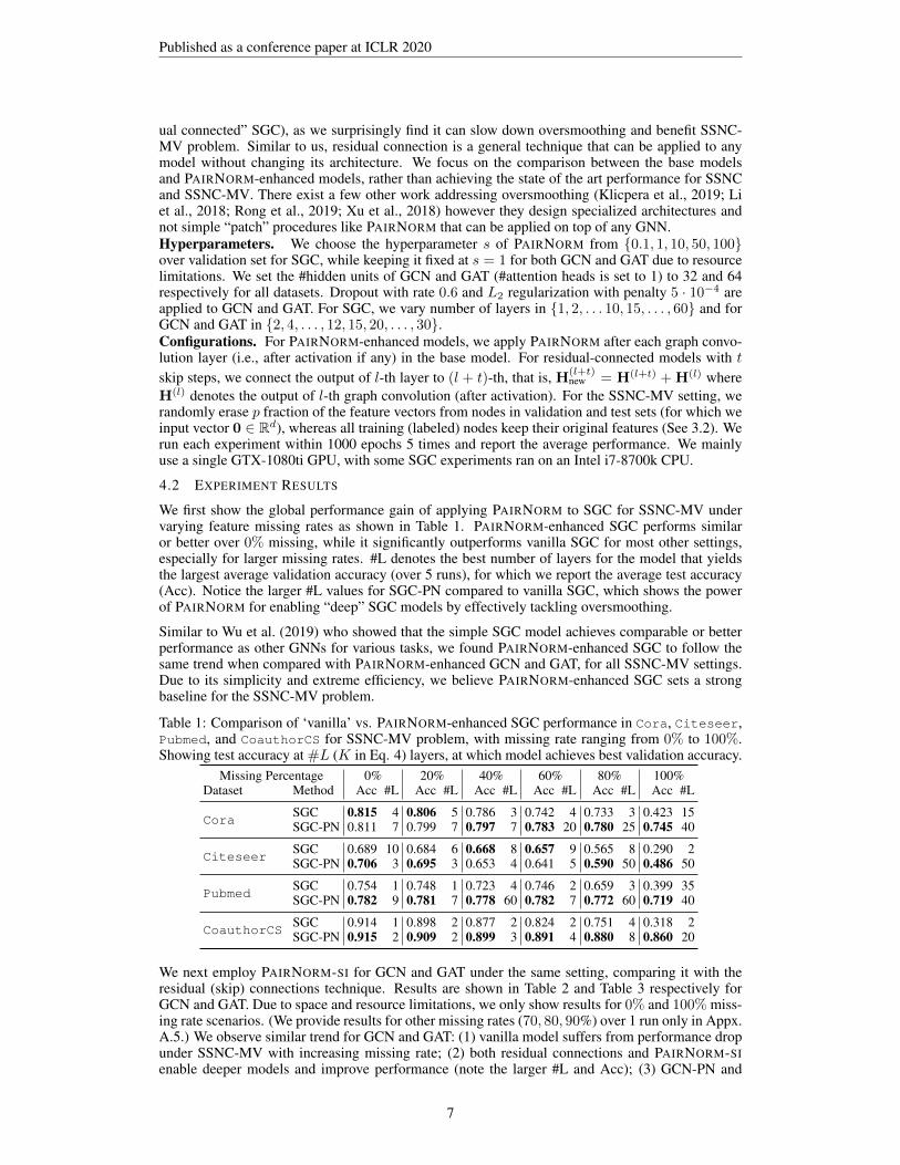
We first show the global performance gain of applying PAIRNORM to SGC for SSNC-MV undervarying feature missing rates as shown in Table 1. PAIRNORM-enhanced SGC performs similaror better over 0% missing, while it significantly outperforms vanilla SGC for most other settings,especially for larger missing rates. #L denotes the best number of layers for the model that yieldsthe largest average validation accuracy (over 5 runs), for which we report the average test accuracy(Acc). Notice the larger #L values for SGC-PN compared to vanilla SGC, which shows the powerof PAIRNORM for enabling “deep” SGC models by effectively tackling oversmoothing.

Similar to Wu et al. (2019) who showed that the simple SGC model achieves comparable or betterperformance as other GNNs for various tasks, we found PAIRNORM-enhanced SGC to follow thesame trend when compared with PAIRNORM-enhanced GCN and GAT, for all SSNC-MV settings.Due to its simplicity and extreme efficiency, we believe PAIRNORM-enhanced SGC sets a strongbaseline for the SSNC-MV problem.

Table 1: Comparison of ‘vanilla’ vs. PAIRNORM-enhanced SGC performance in Cora, Citeseer,Pubmed, and CoauthorCS for SSNC-MV problem, with missing rate ranging from 0% to 100%.Showing test accuracy at #L (K in Eq. 4) layers, at which model achieves best validation accuracy.

Missing Percentage 0% 20% 40% 60% 80% 100%Dataset Method Acc #L Acc #L Acc #L Acc #L Acc #L Acc #L

CoraSGC 0.815 4 0.806 5 0.786 3 0.742 4 0.733 3 0.423 15SGC-PN 0.811 7 0.799 7 0.797 7 0.783 20 0.780 25 0.745 40

CiteseerSGC 0.689 10 0.684 6 0.668 8 0.657 9 0.565 8 0.290 2SGC-PN 0.706 3 0.695 3 0.653 4 0.641 5 0.590 50 0.486 50

PubmedSGC 0.754 1 0.748 1 0.723 4 0.746 2 0.659 3 0.399 35SGC-PN 0.782 9 0.781 7 0.778 60 0.782 7 0.772 60 0.719 40

CoauthorCSSGC 0.914 1 0.898 2 0.877 2 0.824 2 0.751 4 0.318 2SGC-PN 0.915 2 0.909 2 0.899 3 0.891 4 0.880 8 0.860 20

We next employ PAIRNORM-SI for GCN and GAT under the same setting, comparing it with theresidual (skip) connections technique. Results are shown in Table 2 and Table 3 respectively forGCN and GAT. Due to space and resource limitations, we only show results for 0% and 100% miss-ing rate scenarios. (We provide results for other missing rates (70, 80, 90%) over 1 run only in Appx.A.5.) We observe similar trend for GCN and GAT: (1) vanilla model suffers from performance dropunder SSNC-MV with increasing missing rate; (2) both residual connections and PAIRNORM-SIenable deeper models and improve performance (note the larger #L and Acc); (3) GCN-PN and

7


GAT-PN achieve performance that is comparable or better than just using skips; (4) performancecan be further improved (albeit slightly) by using skips along with PAIRNORM-SI.4

Table 2: Comparison of ‘vanilla’ and (PAIRNORM-SI/ residual)-enhanced GCN performance onCora, Citeseer, Pubmed, and CoauthorCS for SSNC-MV problem, with 0% and 100% featuremissing rate. t represents the skip-step of residual connection. (See A.5 Fig. 8 for more settings.)

Dataset Cora Citeseer Pubmed CoauthorCSMissing(%) 0% 100% 0% 100% 0% 100% 0% 100%Method Acc #L Acc #L Acc #L Acc #L Acc #L Acc #L Acc #L Acc #L

GCN 0.821 2 0.582 2 0.695 2 0.313 2 0.779 2 0.449 2 0.877 2 0.452 4

GCN-PN 0.790 2 0.731 10 0.660 2 0.498 8 0.780 30 0.745 25 0.910 2 0.846 12GCN-t1 0.822 2 0.721 15 0.696 2 0.441 12 0.780 2 0.656 25 0.898 2 0.727 12GCN-t1-PN 0.780 2 0.724 30 0.648 2 0.465 10 0.756 15 0.690 12 0.898 2 0.830 20GCN-t2 0.820 2 0.722 10 0.691 2 0.432 20 0.779 2 0.645 20 0.882 4 0.630 20GCN-t2-PN 0.785 4 0.740 30 0.650 2 0.508 12 0.770 15 0.725 30 0.911 2 0.839 20

Table 3: Comparison of ‘vanilla’ and (PAIRNORM-SI/ residual)-enhanced GAT performance onCora, Citeseer, Pubmed, and CoauthorCS for SSNC-MV problem, with 0% and 100% featuremissing rate. t represents the skip-step of residual connection. (See A.5 Fig. 9 for more settings.)

Dataset Cora Citeseer Pubmed CoauthorCSMissing(%) 0% 100% 0% 100% 0% 100% 0% 100%Method Acc #L Acc #L Acc #L Acc #L Acc #L Acc #L Acc #L Acc #L

GAT 0.823 2 0.653 4 0.693 2 0.428 4 0.774 6 0.631 4 0.892 4 0.737 4

GAT-PN 0.787 2 0.718 6 0.670 2 0.483 4 0.774 12 0.714 10 0.916 2 0.843 8GAT-t1 0.822 2 0.706 8 0.693 2 0.461 6 0.769 4 0.698 8 0.899 4 0.842 10GAT-t1-PN 0.787 2 0.710 10 0.658 6 0.500 10 0.757 4 0.684 12 0.911 2 0.844 20GAT-t2 0.820 2 0.691 8 s0.692 2 0.461 6 0.774 8 0.702 8 0.895 4 0.803 6GAT-t2-PN 0.788 4 0.738 12 0.672 4 0.517 10 0.776 15 0.704 12 0.917 2 0.855 30

5 RELATED WORK

Oversmoothing in GNNs: Li et al. (2018) was the first to call attention to the oversmoothing prob-lem. Xu et al. (2018) introduced Jumping Knowledge Networks, which employ skip connectionsfor multi-hop message passing and also enable different neighborhood ranges. Klicpera et al. (2019)proposed a propagation scheme based on personalized Pagerank that ensures locality (via teleports)which in turn prevents oversmoothing. Li et al. (2019) built on ideas from ResNet to use residual aswell as dense connections to train deep GCNs. DropEdge Rong et al. (2019) proposed to alleviateoversmoothing through message passing reduction via removing a certain fraction of edges at ran-dom from the input graph. These are all specialized solutions that introduce additional parametersand/or a different network architecture.Normalization Schemes for Deep-NNs: There exist various normalization schemes proposed fordeep neural networks, including batch normalization Ioffe & Szegedy (2015), weight normalizationSalimans & Kingma (2016), layer normalization Ba et al. (2016), and so on. Conceptually thesehave substantially different goals (e.g., reducing training time), and were not proposed for graphneural networks nor the oversmoothing problem therein. Important difference to note is that largerdepth in regular neural-nets does not translate to more hops of propagation on a graph structure.

6 CONCLUSION

We investigated the oversmoothing problem in GNNs and proposed PAIRNORM, a novel normal-ization layer that boosts the robustness of deep GNNs against oversmoothing. PAIRNORM is fast tocompute, requires no change in network architecture nor any extra parameters, and can be applied toany GNN. Experiments on real-world classification tasks showed the effectiveness of PAIRNORM,where it provides performance gains when the task benefits from more layers. Future work willexplore other use cases of deeper GNNs that could further showcase PAIRNORM’s advantages.

4 Notice a slight performance drop when PAIRNORM is applied at 0% rate. For this setting, and the datasets we have, shallow networksare sufficient and smoothing through only a few (2-4) layers improves generalization ability for the SSNC problem (recall Figure 1 solid lines).PAIRNORM has a small reversing effect in these scenarios, hence the small performance drop.

8


REFERENCES

Jimmy Lei Ba, Jamie Ryan Kiros, and Geoffrey E Hinton. Layer normalization. CoRR,abs/1607.06450, 2016.

Olivier Chapelle, Bernhard Scholkopf, and Alexander Zien. Semi-Supervised Learning. 2006.

William L. Hamilton, Zhitao Ying, and Jure Leskovec. Inductive representation learning on largegraphs. In NIPS, pp. 1024–1034, 2017.

Kaiming He, Xiangyu Zhang, Shaoqing Ren, and Jian Sun. Deep Residual Learning for ImageRecognition. In Proceedings of 2016 IEEE Conference on Computer Vision and Pattern Recog-nition, pp. 770–778. IEEE, 2016.

Sergey Ioffe and Christian Szegedy. Batch normalization: Accelerating deep network training byreducing internal covariate shift. CoRR, abs/1502.03167, 2015.

Thomas N. Kipf and Max Welling. Semi-supervised classification with graph convolutional net-works. In International Conference on Learning Representations (ICLR). OpenReview.net, 2017.

Johannes Klicpera, Aleksandar Bojchevski, and Stephan Gunnemann. Combining neural networkswith personalized pagerank for classification on graphs. In International Conference on LearningRepresentations (ICLR), 2019.

Guohao Li, Matthias Muller, Ali Thabet, and Bernard Ghanem. Can GCNs go as deep as CNNs?CoRR, abs/1904.03751, 2019.

Qimai Li, Zhichao Han, and Xiao-Ming Wu. Deeper Insights into Graph Convolutional Networksfor Semi-Supervised Learning. In Proceedings of the 32nd AAAI Conference on Artificial Intelli-gence, pp. 3538–3545, 2018.

Hoang NT and Takanori Maehara. Revisiting graph neural networks: All we have is low-pass filters.CoRR, abs/1905.09550, 2019.

Meng Qu, Yoshua Bengio, and Jian Tang. Gmnn: Graph markov neural networks. In InternationalConference on Machine Learning, pp. 5241–5250, 2019.

Yu Rong, Wenbing Huang, Tingyang Xu, and Junzhou Huang. The truly deep graph convolutionalnetworks for node classification. CoRR, abs/1907.10903, 2019.

Tim Salimans and Durk P Kingma. Weight normalization: A simple reparameterization to acceleratetraining of deep neural networks. In Advances in Neural Information Processing Systems, pp.901–909, 2016.

Prithviraj Sen, Galileo Namata, Mustafa Bilgic, Lise Getoor, Brian Galligher, and Tina Eliassi-Rad.Collective classification in network data. AI magazine, 29(3):93–93, 2008.

Oleksandr Shchur, Maximilian Mumme, Aleksandar Bojchevski, and Stephan Gunnemann. Pitfallsof graph neural network evaluation. arXiv preprint arXiv:1811.05868, 2018.

Petar Velickovic, Guillem Cucurull, Arantxa Casanova, Adriana Romero, Pietro Li, and YoshuaBengio. Graph attention networks. In International Conference on Learning Representations(ICLR). OpenReview.net, 2018.

Felix Wu, Amauri H. Souza Jr., Tianyi Zhang, Christopher Fifty, Tao Yu, and Kilian Q. Weinberger.Simplifying graph convolutional networks. In ICML, volume 97 of Proceedings of MachineLearning Research, pp. 6861–6871. PMLR, 2019.

Keyulu Xu, Chengtao Li, Yonglong Tian, Tomohiro Sonobe, Ken-ichi Kawarabayashi, and StefanieJegelka. Representation Learning on Graphs with Jumping Knowledge Networks. In Proceedingsof the 35th International Conference on Machine Learning, volume 80, pp. 5453–5462, 2018.

9


A APPENDIX

A.1 DERIVATION OF EQ. 8

TPSD(X) =∑

i,j∈[n]

‖xi − xj‖22 =∑

i,j∈[n]

(xi − xj)T (xi − xj) (13)

=∑

i,j∈[n]

(xTi xi + xT

j xj − 2xTi xj) (14)

= 2n∑i∈[n]

xTi xi − 2

∑i,j∈[n]

xTi xj (15)

= 2n∑i∈[n]

‖xi‖22 − 21T XXT1 (16)

= 2n∑i∈[n]

‖xi‖22 − 2‖1T X‖22 (17)

= 2n2(1

n

n∑i=1

‖xi‖22 − ‖1

n

n∑i=1

xi‖22). (18)

A.2 DATASET STATISTICS

Table 4: Dataset statistics.Name #Nodes #Edges #Features #Classes Label RateCora 2708 5429 1433 7 0.052Citeseer 3327 4732 3703 6 0.036Pubmed 19717 44338 500 3 0.003CoauthorCS 18333 81894 6805 15 0.030

A.3 ADDITIONAL PERFORMANCE PLOTS WITH INCREASING NUMBER OF LAYERS

0 20 40Layers

0.5

1.0

Loss train_loss

val_losstest_loss

0 20 40Layers

0.6

0.8

1.0

Accuracy train_acc

val_acctest_acc

0 20 40Layers

4

6

8

Distance

row_diff

0 20 40Layers

0.2

0.3

0.4

Distance

col_diff

citeseer (random split: 3%/10%/87%) PairNorm Original

0 20 40Layers

0.4

0.6

0.8

1.0

Loss train_loss

val_losstest_loss

0 20 40Layers

0.4

0.6

0.8

Accuracy train_acc

val_acctest_acc

0 20 40Layers

0

2

4

Distance

row_diff

0 20 40Layers

0.02

0.04

Distance

col_diff

pubmed (random split: 3%/10%/87%) PairNorm Original

0 20 40Layers

0.5

1.0

1.5

Loss

train_lossval_losstest_loss

0 20 40Layers

0.4

0.6

0.8

1.0

Accu

racy


0 20 40Layers

0.0

2.5

5.0

7.5

10.0

Dist

ance

row_diff

0 20 40Layers

0.00

0.05

0.10

0.15

0.20

Dist

ance

col_diff

coauthor_CS (random split: 3%/10%/87%) PairNorm Original

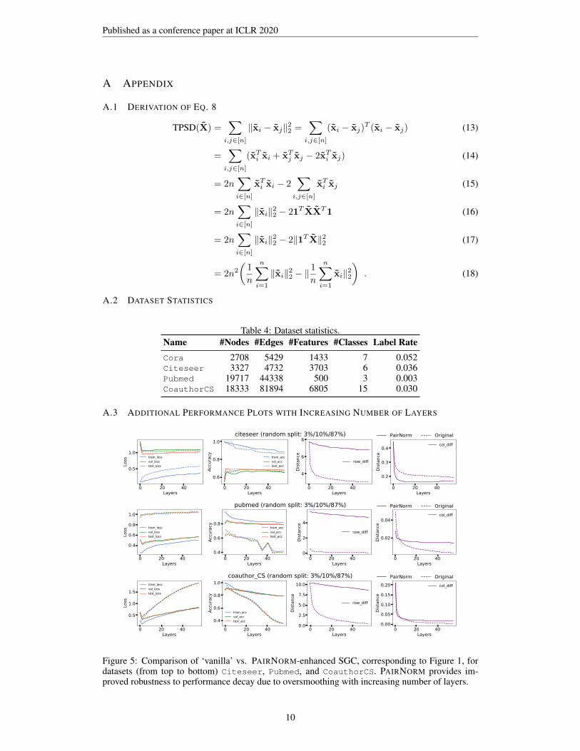
Figure 5: Comparison of ‘vanilla’ vs. PAIRNORM-enhanced SGC, corresponding to Figure 1, fordatasets (from top to bottom) Citeseer, Pubmed, and CoauthorCS. PAIRNORM provides im-proved robustness to performance decay due to oversmoothing with increasing number of layers.

10


10 20 30Layer

0.0

0.2

0.4

0.6

0.8

1.0

Accu

racy

citeseer-GCNPairNorm(SI)Original

10 20 30Layer

0.0

0.2

0.4

0.6

0.8

1.0

Accu

racy

citeseer-GATtrain_accval_acctest_acc

10 20 30Layer

0.0

0.2

0.4

0.6

0.8

1.0

Accuracy

pubmed-GCN

PairNorm(SI)Original

10 20 30Layer

0.0

0.2

0.4

0.6

0.8

1.0

Accuracy

pubmed-GAT


10 20 30Layer

0.0

0.2

0.4

0.6

0.8

1.0

Accu

racy

coauthor_CS-GCN


10 20 30Layer

0.0

0.2

0.4

0.6

0.8

1.0

Accu

racy

coauthor_CS-GAT


Figure 6: Comparison of ‘vanilla’ (dashed) vs. PAIRNORM-enhanced (solid) GCN (left) and GAT(right) models, corresponding to Figure 3, for datasets (from top to bottom) Citeseer, Pubmed, andCoauthorCS. PAIRNORM provides improved robustness against performance decay with increasingnumber of layers.

11


A.4 ADDITIONAL PERFORMANCE PLOTS WITH INCREASING NUMBER OF LAYERS UNDERSSNC-MV WITH p = 1

0 20 40Layer

0.0

0.2

0.4

0.6

0.8

1.0

Accu

racy

citeseer-SGC

0 10 20 30Layer

0.0

0.2

0.4

0.6

0.8

1.0

Accu

racy

citeseer-GCNPairNorm(SI)Original

10 20 30Layer

0.0

0.2

0.4

0.6

0.8

1.0

Accu

racy

citeseer-GATtrain_accval_acctest_acc

0 20 40Layer

0.0

0.2

0.4

0.6

0.8

1.0

Accuracy

pubmed-SGC

10 20 30Layer

0.0

0.2

0.4

0.6

0.8

1.0Ac

curacy

pubmed-GCN


10 20 30Layer

0.0

0.2

0.4

0.6

0.8

1.0

Accuracy

pubmed-GATtrain_accval_acctest_acc

0 20 40Layer

0.0

0.2

0.4

0.6

0.8

1.0

Accu

racy

coauthor_CS-SGC

10 20 30Layer

0.0

0.2

0.4

0.6

0.8

1.0

Accu

racy

coauthor_CS-GCN


10 20 30Layer

0.0

0.2

0.4

0.6

0.8

1.0Ac

cura

cycoauthor_CS-GAT


Figure 7: Comparison of ‘vanilla’ (dashed) vs. PAIRNORM-enhanced (solid) (from left to right)SGC, GCN, and GAT model performance under SSNC-MV for p = 1, corresponding to Figure 4,for datasets (from top to bottom) Citeseer, Pubmed, and CoauthorCS. Green diamond symbolsdepict the layer at which validation accuracy peaks. PAIRNORM boosts overall performance byenabling more robust deep GNNs.

12


A.5 ADDITIONAL EXPERIMENTS UNDER SSNC-MV WITH INCREASING MISSINGFRACTION p

In this section we report additional experiment results under the SSNC-MV setting with varyingmissing fraction, in particular p = {0.7, 0.8, 0.9, 1} and also report the base case where p = 0 forcomparison.

Figure 8 presents results on all four datasets for GCN vs. PAIRNORM-enhanced GCN (denotedPN for short). The models without any skip connections are denoted by *-0, with one-hop skipconnection by *-1, and with one and two-hop skip connections by *-2. Barcharts on the right reportthe best layer that each model produced the highest validation accuracy, and those on the left reportthe corresponding test accuracy. Figure 9 presents corresponding results for GAT.

We discuss the take-aways from these figures on the following page.

GCN-0 PN -0GCN-1 PN -1GCN-2 PN -2GCN-0 PN -0GCN-1 PN -1GCN-2 PN -2GCN-0 PN -0GCN-1 PN -1GCN-2 PN -2GCN-0 PN -0GCN-1 PN -1GCN-2 PN -2GCN-0 PN -0GCN-1 PN -1GCN-2 PN -2

0

5

10

0% missing 70% missing 80% missing 90% missing 100% missing

Best Layer


0.6

0.7

0.8


Test Acc cora GCN


0

5

10


Best Layer


0.4

0.6


Test Acc citeseer GCN


0

5

10


Best Layer


0.4

0.6

0.8


Test Acc pubmed GCN


0

5

10


Best Layer


0.4

0.6

0.8


Test Acc coauthor_CS GCN

Figure 8: Supplementary results to Table 2 for GCN on (from top to bottom) Cora, Citeseer,Pubmed, and CoauthorCS.

13


We make the following observations based on Figures 8 and 9:

• Performance of ‘vanilla’ GCN and GAT models without skip connections (i.e., GCN-0 andGAT-0) drop monotonically as we increase missing fraction p.

• PAIRNORM-enhanced ‘vanilla’ models (PN-0, no skips) perform comparably or better thanGCN-0 and GAT-0 in all cases, especially as p increases. In other words, with PAIRNORMat work, model performance is more robust against missing data.

• Best number of layers for GCN-0 as we increase p only changes between 2-4. For GAT-0,it changes mostly between 2-6.

• PAIRNORM-enhanced ‘vanilla’ models (PN-0, no skips) can go deeper, i.e., they can lever-age a larger range of #layers (2-12) as we increase p. Specifically, GCN-PN-0 (GAT-PN-0)uses equal number or more layers than GCN-0 (GAT-0) in almost all cases.

• Without any normalization, adding skip connections helps—GCN/GAT-1 and GCN/GAT-2are better than GCN/GAT-0, especially as we increase p.

• With PAIRNORM but no-skip, performance is comparable or better than just adding skips.• Adding skips on top of PAIRNORM does not seem to introduce any notable gains.

In summary, simply employing our PAIRNORM for GCN and GAT provides robustness againstoversmoothing that allows them to go deeper and achieve improved performance under SSNC-MV.

GAT-0 PN -0GAT-1 PN -1GAT-2 PN -2GAT-0 PN -0GAT-1 PN -1GAT-2 PN -2GAT-0 PN -0GAT-1 PN -1GAT-2 PN -2GAT-0 PN -0GAT-1 PN -1GAT-2 PN -2GAT-0 PN -0GAT-1 PN -1GAT-2 PN -2

0

5

10


Best Layer


0.6

0.8


Test Acc cora GAT


0

5

10


Best Layer


0.4

0.6


Test Acc citeseer GAT


0

5

10


Best Layer


0.5

0.6

0.7

0.8


Test Acc pubmed GAT


0

5

10


Best Layer


0.7

0.8

0.9


Test Acc coauthor_CS GAT

Figure 9: Supplementary results to Table 3 for GAT on (from top to bottom) Cora, Citeseer,Pubmed, and CoauthorCS.

14


A.6 CASE STUDY: ADDITIONAL MEASURES FOR PAIRNORM AND PAIRNORM-SI WITH SGCAND GCN

To better understand why PAIRNORM and PAIRNORM-SI are helpful for training deep GNNs, wereport additional measures for (SGC and GCN) with (PAIRNORM and PAIRNORM-SI) over theCora dataset. In the main text, we claim TPSD (total pairwise squared distances) is constant acrosslayers for SGC with PAIRNORM (for GCN/GAT this is not guaranteed because of the influence ofactivation function and dropout layer). In this section we empirically measure pairwise (squared)distances for both SGC and GCN, with PAIRNORM and PAIRNORM-SI.

A.6.1 SGC WITH PAIRNORM AND PAIRNORM-SI

To verify our analysis of PAIRNORM for SGC, and understand how the variant of PAIRNORM(PAIRNORM-SI) works, we measure the average pairwise squared distance (APSD) as well as theaverage pairwise distance (APD) between the representations for two categories of node pairs: (1)connected pairs (nodes that are directly connected in graph) and (2) random pairs (uniformly ran-domly chosen among the node set). APSD of random pairs reflects the TPSD, and APD of randompairs reflects the total pairwise distance (TPD). Under the homophily assumption of the labels w.r.t.the graph structure, we want APD or APSD of connected pairs to be small while keeping APD orAPSD of random pairs relatively large.

The results are shown in Figure 10. Without normalization, SGC suffers from fast diminishing APDand APSD of random pairs. As we have proved, PAIRNORM normalizes APSD to be constant acrosslayers, however it does not normalize APD, which appears to decrease linearly with increasing num-ber of layers. Surprisingly, although PAIRNORM-SI is not theoretically proved to have a constantAPSD and APD, empirically it achieves more stable APSD and APD than PAIRNORM. We werenot able to prove this phenomenon mathematically, and leave it for further investigation.

0 10 20 30 40 500

10

20

30

Averag

e sq

uared distan

ce

SGCconnected pairsrandom pairs

0 10 20 30 40 50Layers

0

1

2

3

4

5

6

Averag

e distan

ce

0 10 20 30 40 500

10

20

30

SGC + PairNorm

connected pairsrandom pairs

0 10 20 30 40 50Layers

0

1

2

3

4

5

6

0 10 20 30 40 500

10

20

30

SGC + PairNorm-SI


0 10 20 30 40 50Layers

1

2

3

4

5

6

Dataset: cora

Figure 10: Measuring average distance (squared and not-squared) between representations at eachlayer for SGC, SGC with PAIRNORM, and SGC with PAIRNORM-SI. The setting is the same withFigure 1 and they share the same performance.

APD does not capture the full information of the distribution of pairwise distances. To show howthe distribution changes by increasing number of layers, we use Tensorboard to plot the histogramsof pairwise distances, as shown in Figure 11. Comparing SGC and SGC with PAIRNORM, addingPAIRNORM keeps the left shift (shrinkage) of the distribution of random pair distances much slowerthan without normalization, while still sharing similar behavior of the distribution of connectedpairwise distances. PAIRNORM-SI seems to be more powerful in keeping the median and mean ofthe distribution of random pair distances stable, while “spreading” the distribution out by increasingthe variance. The performance of PAIRNORM and PAIRNORM-SI are similar, however it seems thatPAIRNORM-SI is more powerful in stabilizing TPD and TPSD.

15


distr. of random pair distances

Layers

Distance

Layers

SGC SGC + PairNorm SGC + PairNorm-SI distr. of connected pair distances distr. of connected pair distances

distr. of random pair distances distr. of random pair distances

Distance Distance

Dataset: Coradistr. of connected pair distances

Figure 11: Measuring distribution of distances between representations at each layer for SGC, SGCwith PAIRNORM, and SGC with PAIRNORM-SI. Supplementary results for Figure 10.

A.6.2 GCN WITH PAIRNORM AND PAIRNORM-SI

0 2 4 6 8 100.000

0.002

0.004

0.006

0.008

0.010

Averag

e sq

uared distan

ce

GCNconnected pairsrandom pairs

0 2 4 6 8 10Layers

0.00

0.02

0.04

0.06

0.08

0.10

Averag

e distan

ce

0 2 4 6 8 100

20406080

100120

GCN + PairNorm


0 2 4 6 8 10Layers

2

4

6

8

10

0 2 4 6 8 100.0

0.2

0.4

0.6

0.8GCN + PairNorm-SI


0 2 4 6 8 10Layers

0.2

0.4

0.6

0.8

Dataset: cora

Figure 12: Measuring average distance (squared and not-squared) between representations at eachlayer for GCN, GCN with PAIRNORM, and GCN with PAIRNORM-SI. We trained three 12-layerGCNs with #hidden=128 and dropout=0.6 in 1000 epochs. Respective test set accuracies are31.09%, 77.77%, 75.09%. Note that the scale of distances is not comparable across models, sincethey have learnable parameters that scale these distances differently.

The formal analysis for PAIRNORM and PAIRNORM-SI is based on SGC. GCN (and other GNNs)has learnable parameters, dropout layers, and activation layers, all of which complicate direct math-ematical analyses. Here we perform similar empirical measurements for pairwise distances to geta rough sense of how PAIRNORM and PAIRNORM-SI work with GCN based on the Cora dataset.Figures 12 and 13 demonstrate how PAIRNORM and PAIRNORM-SI can help train a relatively deep(12 layers) GCN.

Notice that oversmoothing occurs very quickly for GCN without any normalization, where both con-nected and random pair distances reach zero (!). In contrast, GCN with PAIRNORM or PAIRNORM-SI is able to keep random pair distances relatively apart while allowing connected pair distancesto shrink. As also stated in main text, using PAIRNORM-SI for GCN and GAT is relatively more

16


stable than using PAIRNORM in general cases (notice the near-constant random pair distances inthe rightmost subfigures). There are several possible explanations for why PAIRNORM-SI is morestable. First, as shown in Figure 10 and Figure 12, PAIRNORM-SI not only keeps APSD stable butalso APD, further, the plots of distributions of pairwise distances (Figures 11 and 13) also show thepower of PAIRNORM-SI (notice the large gap between smaller connected pairwise distances and thelarger random pairwise distances). Second, we conjecture that restricting representations to resideon a sphere can make training stable and faster, which we also observe empirically by studying thetraining curves. Third, GCN and GAT tend to overfit easily for the SSNC problem, due to manylearnable parameters across layers and limited labeled input data, therefore it is possible that addingmore restriction on these models helps reduce overfitting.

GCN GCN + PairNorm GCN + PairNorm-SI Dataset: Cora

distr. of connected pair distances distr. of connected pair distancesdistr. of connected pair distances

distr. of random pair distances distr. of random pair distances distr. of random pair distances

Layers

Distance

Layers

Distance Distance

Figure 13: Measuring distribution of distances between representations at each layer for GCN, GCNwith PAIRNORM, and GCN with PAIRNORM-SI. Supplementary results for Figure 12.

All in all, these empirical measurements as illustrated throughout the figures in this section demon-strates that PAIRNORM and PAIRNORM-SI successfully address the oversmoothing problem fordeep GNNs. Our work is the first to propose a normalization layer specifically designed for graphneural networks, which we hope will kick-start more work in this area toward training more robustand effective GNNs.

17

Documents

PAIRNORM: TACKLING OVERSMOOTHING IN GNNS