PAGE PROOFS Linear inequalities programming and linear · PDF fileLinear inequalities To begin our work in linear programming, we fi rst have to develop some skills with linear inequalities

15Linear inequalities

and linear programming

15.1 Kick off with CAS

15.2 Linear inequalities

15.3 Simultaneous linear inequalities

15.4 Linear programming

15.5 Applications

15.6 Review

c15LinearInequalitiesAndLinearProgramming.indd 744 12/09/15 4:58 AM

UNCORRECTED PAGE P

ROOFS

Please refer to the Resources tab in the Prelims section of your eBookPlUs for a comprehensive step-by-step guide on how to use your CAS technology.

15.1 Kick off with CASShading regions with CAS

When graphing a linear equation, the Cartesian plane is split into two regions (one on either side of the line). Linear inequalities replace the equals sign in an equation with an inequality sign (≤, ≥, < or >). This means that one of the regions the Cartesian plane is split into satisfi es the inequality, whereas the other region doesn’t satisfy the inequality.

1 Using CAS, sketch the graph of y < 12 − 3x.

2 Using any appropriate method, determine which region of the graph (shaded or unshaded) satisfi es the inequality, i.e. on which side of the line do the points make the inequality true?

3 Using CAS, sketch the graphs of y < 12 − 3x and y < 12 − x3

on the same set of axes.

4 Determine the point of intersection of the two lines sketched in question 3.

5 Determine which region of the graphs plotted in question 3 is the required region; that is, which region satisfi es both of the inequalities.

6 Use CAS to plot the following system of linear inequalities:

y < 10 – x

y < 4x

y ≥ 0

7 Use CAS to fi nd all the corner points of the required region for the system of linear inequalities plotted in question 6.


UNCORRECTED PAGE P

ROOFS

Linear inequalitiesTo begin our work in linear programming, we fi rst have to develop some skills with linear inequalities. Recall that linear equations come in two forms:

y = mx + cand ax + by = c.

For example, y = 3x – 4 is a linear equation, as is 3x + 4y = –9.

Linear inequalities also have two forms:

y < mx + cand ax + by < c.

For example, y < 3x – 4 is a linear inequality, as is 3x + 4y ≥ –9. It is the second form of equation that we will be chiefl y working with in this topic. The only difference between equations and inequalities is that the equals sign (=) is replaced with an ‘inequality’ sign. The possible inequality signs are:

≥ greater than or equal to

> greater than

< less than

≤ less than or equal to.

graphing a linear inequalityThe steps for graphing a linear inequality are the same as those for linear equations, with one extra step. The graph of an inequality is a region or half-plane while the graph of a linear equation is a straight line.

Step 1. Temporarily treat the inequality as an equation to fi nd the boundary of the region.

Step 2. Find two points using the equation to assist in graphing the boundary. Pick any value of x and fi nd the corresponding value of y. Pick another value of x and fi nd the corresponding value of y. This value of x should be reasonably far away from the fi rst one chosen.

Step 3. Plot the points from step 2 and join them with a straight line. Extend the straight line to the extent of your graph paper. A dashed line should be used for a < or > inequality and a solid line for a ≤ or ≥ inequality.

Step 4. Shade in a region, either above the graph or below the graph, depending upon the inequality sign given. The convention is to shade the region not required. Any point inside the shaded region is not a solution to the inequation. Thus, the unshaded (or clear) area is called the solution region or the feasible region. Note: Some CAS calculators shade the solution region.

15.2

Graph the linear inequality 3x + 4y ≥ –9.

tHinK WritE/DrAW

1 Find the boundary of the region.(a) Write the inequality as an equation.(b) Pick any value for x and fi nd the

corresponding y-value.

The boundary is 3x + 4y = –9. Let x = 03(0) + 4y = −9

WorKed eXampLe 111

Unit 4

AOS M4

Topic 2

Concept 1

Variables, constraints and inequalitiesConcept summary Practice questions

Unit 4

AOS M4

Topic 2

Concept 2

Graphing inequalitiesConcept summary Practice questions

InteractivityLinear inequalities in two variablesint-6488

746 maThs quesT 12 FurTher maThemaTiCs VCe units 3 and 4


UNCORRECTED PAGE P

ROOFS

Note that in Worked example 1, because the inequality was ‘greater than or equal to’, the solution region also included the straight line itself (shown with a solid line).

If the inequality had been just ‘greater than’ then the region would not have included the straight line points (a dashed line would have been used).

However, most problems in this topic will be of the ‘... equal to’ type.

A faster alternative to steps 1(b) to 1(e) in Worked example 1 is to find the x- and y-intercepts to the boundary line. First substitute x = 0 and find the corresponding

(c) Substitute the x-value into the equation and solve for y.

4y = −9

y = −94

= –2.25. First point is (0, –2.25)

(d) Pick another value for x and find the corresponding y-value.

(e) Substitute the x-value into the equation and solve for y.

Let x = 93(9) + 4y = −9

27 + 4y = −9 4y = −36 y = −9. Second point is (9, −9)

(f) Plot the two points on a graph and join them with a straight line. A solid line is used since the inequality contains a ≥ sign. Observe how the line is extended the full extent of the graph paper. This line divides the coordinate plane into two ‘half-planes’.

10

5

–5

–10

5 10–5–10 x

y

0

2 Find the required region.(a) Select a test point above the line to work

out the region or half-plane required.(b) Substitute the x- and y-values into

the inequality. If the inequality is satisfied (or true) then the half-plane containing the test point is required. If not, the other half-plane is required.

Test point: (5, 0) 3x + 4y ≥ −93(5) + 4(0) ≥ −9?15 ≥ –9 is true, so the region required is above the line.

3 Shade in the region not required (that is, the half-plane below the line) and add the legend.

10

5

–5

–10

5 10–5–10 0 x

y

Region required

Topic 15 Linear inequaLiTies and Linear programming 747


UNCORRECTED PAGE P

ROOFS

Graph the inequality 3x – 4y < 12 using the x- and y-intercept method and show that (5, 2) is a solution.

tHinK WritE/DrAW

1 Find the boundary.(a) Write the equation of the boundary.(b) Find the y-intercept by substituting

x = 0 into the equation and fi nding the corresponding value of y.

(c) Find the x-intercept by substituting y = 0 into the equation and fi nding the corresponding value of x.

The boundary of the region is 3x – 4y = 12. When x = 0, 3(0) − 4y = 12 −

4y = 12

y = −3 Point is (0, −3) When y = 0, 3x − 4(0) = 12 3x = 12 x = 4 Point is (4, 0)

–3

40

y

x

(d) Plot the two points on a graph and join them with a straight, dashed line.

2 Find the required region.(a) Select a test point, say (0, 0), to

work out the half-plane required.(b) Substitute the x- and y-values into

the inequality. If the inequality is satisfi ed (or true) then the half-plane containing the test point is required. If not, the other half-plane is required.

Test point: (0, 0) 3x − 4y < 123(0) + 4(0) < 12?0 < 12 is true, so the region required is above the line.

3 Shade in the region not required, that is, the half-plane below the line.

–3

4 50

2

y

x

Regionrequired

4 Plot the given point (5, 2) to see whether it is within the required region.

Alternatively: Substitute the co-ordinates of the given point (5, 2) into the inequality to see if it will make a true statement.

The point (5, 2) lies inside the unshaded region. Therefore, it is a solution to the inequality.

Test point (5, 2):3(5) – 4(2) < 12?

15 – 8 < 12?7 < 12 is true, therefore (5, 2) is a solution to the inequality.

WorKed eXampLe 222

value of y and then substitute y = 0 and fi nd the corresponding value of x. Plot these two points to get the straight line. This is called the x- and y-intercept method.



UNCORRECTED PAGE P

ROOFS

Linear inequalities1 WE1 Graph the solution to the linear inequality 4x + 7y ≤ 28.

2 Graph the solution to the linear inequality 50x – 65y ≥ 650.

3 WE2 Graph the inequality 7x – 12y ≤ 84 and show that (4, –3) is a solution.

4 Graph the inequality –5x – 3y ≥ 20 and show that (–10, –5) is a solution.


6 Graph the solutions to the following linear inequalities.

a 6x + 2y > 12 b 4x + y ≤ 5c 3x + 2y ≥ 0 d x – y > 20

7 Graph the inequality 4x + 5y ≤ 20 and show that (1, 1) is a solution.

8 Graph the inequality 6x – 4y + 20 > 0 and show that (10, 5) is a solution.

9 Graph the inequality 2x + 3y ≥ 6 and show that (7, 0) is a solution.

10 Graph the inequality 1.5x – 3.5y < 2.7.

11 Which one or more of the points below is/are solutions to the inequality in question 10?

A (5, –5) B (5, 5) C (10, 2) D (–1, –2) E (10, 6)

12 Graph the inequality 20x + 30y ≥ 300.

13 The point which is not a solution to the inequality in question 12 is:

A (10, 5) B (5, 8) C (5, 5) D (1, 10) E (2, 10)


15 Graph the linear inequality 2x + 7y ≤ 0 and show that (–5, 1) is inside the solution region.

16 Graph the solution to the linear inequality –1.8x + 0.4y ≤ 14.4.

ExErCisE 15.2

PrACtisE

ConsoliDAtE

MAstEr

15.3 Simultaneous linear inequalitiesAs with linear equations, it is possible to solve groups of linear inequalities simultaneously; that is, to find the solution that satisfies more than one inequality at the same time. You may recall that there are several methods for solving simultaneous linear equations; some of these techniques will be useful for inequations. Note that simultaneous linear inequalities are also called systems of linear inequalities.

graphical solution of simultaneous linear inequalitiesTo solve for two linear inequalities, follow these steps.

Step 1. Graph the solution for the first linear inequality.

Step 2. Graph the solution for the second linear inequality.

Step 3. The solution to both inequalities is the intersection of the solution regions from Steps 1 and 2.

InteractivityGraphing a linear inequality (simultaneous inequalities) int-6283



UNCORRECTED PAGE P

ROOFS

Find the solution to the simultaneous linear inequalities:

x + 2y2y2 ≤ 10 [1]2x + y ≤ 10 [2]

tHinK WritE/DrAW

1 Write the boundary equation for region [1].

The boundary for region [1] is x + 2y = 10.

2 Find the x- and y-intercepts of the boundary line.

When x = 0, 0 + 2y = 10 y = 5 (0, 5)When y = 0,

x + 2(0) = 10 x = 10 (10,

0)

3 Plot the straight line and determine the region of the solution by using a test point.

Test point: (0, 0)x + 2y ≤ 10

0 + 2(0) ≤ 10 is true, so (0, 0) is inside the solution region.

4 Repeat steps 1–3 for region [2]. The boundary for region [2] is 2x + y = 10. When x = 0, 2(0) + y = 10 y = 10 (0, 10)

When y = 0, 2x + 0 = 10 2x = 10 x = 5 (5, 0)Test point: (0, 0)

2x + y ≤ 102(0) + 0 ≤ 10 is true, so(0, 0) is inside the region.

5 Determine the overlapping areas of the two regions. This can be done graphically, by showing the two regions on the one set of axes. The clear area is the overlap of the two solution regions and represents the solution to the simultaneous linear inequalities.

10

–5

5 10–5 0 x

y

Region required

5

Region required

10

5

–5

5 10–5 0 x

y

10

5

–5

5 10–5 0 x

y

Region required

WorKed eXampLe 333



UNCORRECTED PAGE P

ROOFS

Note that in Worked example 3, there were three non-solution regions:

1. the region above and to the left of the fi rst line,2. the region above and to the right of the second line, and3. the region where the two exclusion zones overlap.

Notes

1. The convention of shading the region that is not required makes it easier to identify overlapping exclusion zones; however, CAS may shade the required region. Use test points to confi rm which style is being used.

2. In this topic, where more exclusion zones overlap, the regions will be shown in increasingly darker shades of blue.

3. In subsequent sections, we examine systems of three or more linear inequalities, but the methods are identical.

4. Examination questions usually ask for the required region to be shaded. Always read the question carefully and include a legend with your graphical solutions.

Find the solution to the system of linear inequalities at right.

x + 2y2y2 ≤ 5 [1]4x + 3y ≤ 12 [2]x ≥ 0 [3]y ≥ 0 [4]

tHinK WritE/DrAW

1 Write the boundary equations for each region and fi nd the intercepts or relevant information to sketch each line.

The boundary for region [1] is x + 2y = 5.When x = 0, y = 2.5 (0, 2.5)When y = 0, x = 5 (5, 0)The boundary for region [2] is 4x + 3y = 12.When x = 0, y = 4 (0, 4)When y = 0, x = 3 (3, 0)The boundary for region [3] is x = 0.This is a vertical line through x = 0.The boundary for region [4] is y = 0.This is a horizontal line through y = 0.

2 Use test points to identify the required region for each inequality. Note that (0, 0) cannot be used for inequalities [3] and [4] as this point lies on the boundary for each.

For x + 2y ≤ 5: Test point (0, 0)(0) + 2(0) ≤ 5 is true, so (0, 0) is inside the region.For 4x + 3y ≤ 12: Test point (0, 0)4(0) + 3(0) ≤ 12 is true, so (0, 0) is inside the region.For x ≥ 0: Test point (1, 0)

1 ≥ 0, so (1, 0) is inside the region.For y ≥ 0: Test point (0, 2)

2 ≥ 0, so (0, 2) is inside the region.

3 Show each region on the one set of axes. Remember to shade the region not required in each case. The clear area is the solution for this system of inequalities.

4

2

1 3 50 x

y

12 –2

Region required

WorKed eXampLe 444



UNCORRECTED PAGE P

ROOFS

Observe that the solution region is a polygon (in this case a quadrilateral). This is a feature of all of the subsequent problems we will study. Generally speaking, if there are n linear inequalities, we can get a polygon of up to n sides. The solution region is also called the feasible region.

Sometimes the overlap between solution regions is not so obvious.

Find the solution to the following system of linear inequalities.

8x + 5y ≤ 40 [1]3x + 4y ≤ 12 [2]2x + y ≤ 6 [3]x ≥ 0 [4]y ≥ 0 [5]

tHinK WritE/DrAW

1 Find the intercepts of the boundary lines and use a test point to determine which side of the boundary to shade. Note that inequations [4] and [5] indicate that we are interested only in positive values of x and y, as well as when x or y equal zero; that is, non-negative values of x and y.

Region [1]: 8x + 5y = 40 has intercepts of (0, 8) and (5, 0) with a test point of (0, 0) inside the feasible region.Region [2]: 3x + 4y = 12 has intercepts (0, 3) and (4, 0) with a test point of (0, 0) inside the feasible region.Region [3]: 2x + y = 6 has intercepts (0, 6) and (3, 0) with a test point of (0, 0) inside the feasible region.

2 Graph the solution to each of the inequalities on the same set of axes. Remember to shade the regions not required. The clear area is the solution region for this system of inequalities.Note: When we are interested in only positive values of x and y, it is usual not to extend lines beyond the axes, or to shade in the negative quadrants.

3

6

8

3 540 x

y

Region required

WorKed eXampLe 555

What Worked example 5 indicates is that not all the inequalities are part of the solution region. In Worked example 5, inequality [1] has no role to play. However, this is usually not obvious until all the inequalities have been graphed.

Note: In the exercises that follow, you will notice that the majority of the systems contain inequalities x ≥ 0 and y ≥ 0. These two inequalities describe the fi rst quadrant of the Cartesian plane, including the origin and the positive sections of the x- and y-axis.



UNCORRECTED PAGE P

ROOFS

Simultaneous linear inequalities1 WE3 Graph the solution to the following system of inequalities.

2x − 3y ≤ 125x + 4y ≤ 40

2 Graph the solution to the following system of inequalities.−4x + y ≥ 12x + 3y ≤ 21

3 WE4 Graph the solution to the following system of inequalities.2x + 3y ≤ 243x + 2y ≤ 18x ≥ 0y ≥ 0

4 Graph the solution to the following system of inequalities.5x + 12y ≤ 1206x + 5y ≤ 60x ≥ 0y ≥ 0

5 WE5 Graph the solution to the following system of inequalities. 2x + y ≤ 2x + 3y ≤ 33x + 2y ≤ 6x ≥ 0y ≥ 0

6 Graph the solution to the following system of inequalities.3x + 5y ≤ 75x + y ≤ 2010y + 4x ≤ 100x ≥ 0y ≥ 0

For questions 7–15, graph the solution to the given system of linear inequalities.

7 5x + 3y ≤ 153x + 5y ≤ 15

8 5x + 3y ≤ 15−x + y ≤ 2

9 2x + 3y ≤ 62x − 5y ≥ 10

10 6x + 8y ≥ 03x + 4y ≤ 12

11 8x + 3y ≤ 245x + 7y ≤ 35x ≥ 0y ≥ 0

12 8x + 2y ≤ 164x + 5y ≤ 20x ≥ 0y ≥ 0

13 2x + 5y ≤ 107x + 3y ≤ 21x ≥ 0y ≥ 0

14 3x + 2y ≥ 6x + y ≤ 6−2x + 6y ≤ 6x ≥ 0y ≥ 0

15 10x + 3y ≤ 307x + 5y ≤ 353x + 7y ≤ 21x ≥ 0y ≥ 0

16 Modify the first and third inequalities of question 15 so that ‘less than or equal to’ becomes ‘greater than or equal to’ and re-solve.

17 3x + y ≥ 3 5x + 4y ≤ 20 14x + 4y ≤ 28 x ≥ 0 y ≥ 0The point that is part of the solution to the system of linear inequalities above is:

A (1, 5) B (2, 1) C (3, 0) D (1, 3) E (0, 6)

ExErCisE 15.3

PrACtisE

ConsoliDAtE

MAstEr



UNCORRECTED PAGE P

ROOFS

18 A rectangular swimming pool is constructed with the following restrictions in mind:

a Write the restrictions in terms of algebraic inequalities.b Graph the solution to the system of linear inequalities.c Show that a pool of length of 10 m and a width of 10 m is not possible.

Linear programmingNow that you have the skills necessary for graphing inequations, you are in a position to tackle the main purpose of this topic: solving linear programming problems.

What is a linear programming problem? It consists of 3 vital components:

1. a set of variables (in this topic we shall always have exactly two) called decision variables

2. a set of restrictions or constraints on the values of these variables3. a function (called the objective function) of these two variables that we wish to

make either as large as possible (maximise) or as small as possible (minimise).

Generally, by convention, x and y are used to represent the two variables.

The decision variablesIn the general linear programming problem there are many variables. In the Further Mathematics course we are restricted to only two, so that Cartesian graphical methods can be employed. In real-life engineering situations (linear programming is part of a study known as industrial engineering), linear programming problems with up to 100 variables have been solved. In some cases the variables must be integers (whole numbers), while in other problems they can take on any real value; sometimes it may not be obvious which case applies.

The constraintsThe constraints are expressed as a set of inequalities, similar to those we encountered in the previous section. Let us consider a scenario which we will be working on in the next few examples. In this case there will be three constraints; but the procedures outlined in Worked examples 6, 7 and 8 would be exactly the same as for only two constraints.

15.4

1. The perimeter is to be at least 20 metres.

2. The difference between the length (y metres) and the width (x metres) must be 5 metres or more.

3. Neither length nor width can exceed 15 metres.



UNCORRECTED PAGE P

ROOFS

A company produces clothes washers and dryers.

Each product requires assembly in three different factories before it can be sold.

Each factory requires different amounts of time to work on each washer or dryer, according to the following table.

Use of time Factory A Factory B Factory C

Time spent on washer 2 hours 4 hours 2 hours

Time spent on dryer 1 hour 2 hours 2 hours

Maximum time the factory is available each day

24 hours 16 hours 12 hours

From this table we conclude that it takes 2 + 4 + 2 = 8 hours to produce a single washer and 1 + 2 + 2 = 5 hours to produce a single dryer. Convert these times into a series of constraints. The aim is to investigate the number of washers and dryers produced each day.

tHinK WritE

1 Identify the decision variables.

(a) What is the number of washers produced each day?

(b) What is the number of dryers produced each day? (You could just as easily choose x for dryers and y for washers.)

Let x = number of washers made daily

Let y = number of dryers made daily

2 Consider the daily capacity of factory A. For factory A:Time spent on x washers = 2x hoursTime spent on y dryers = 1y hoursMaximum time spent on items = 24 hours

3 Turn this into an inequality. (Because 24 hours is a maximum, we could use less time, therefore the ‘less than or equal sign’ is used.)

2x + 1y ≤ 24

4 Repeat steps 2 and 3 for factory B. For factory B:Time spent on x washers = 4x hoursTime spent on y dryers = 2y hoursMaximum time spent on items = 16 hours4x + 2y ≤ 16

5 Repeat steps 2 and 3 for factory C. For factory C:Time spent on x washers = 2x hoursTime spent on y dryers = 2y hoursMaximum time spent on items = 12 hours2x + 2y ≤ 12

6 Consider other (physical) constraints.Obviously, both x and y cannot be negative, since they represent a number of washers and dryers.

x ≥ 0y ≥ 0

WorKed eXampLe 666



UNCORRECTED PAGE P

ROOFS

It may or may not be reasonable to insist that x and y be integers. Is it possible to make 2.4 washers in a day? The answer to this is not necessarily obvious from the question, so for now, assume that x and y can take any positive value.

graphing the constraintsThe next stage in the process is to graph the constraints as we did in the previous section on simultaneous linear inequalities, and determine the overlapping solution region.

7 List all the constraints together. 2x + y ≤ 244x + 2y ≤ 162x + 2y ≤ 12x ≥ 0y ≥ 0

Graph the constraints from Worked example 6.

tHinK WritE/DrAW

1 List the constraints. 2x + y ≤ 244x + 2y ≤ 162x + 2y ≤ 12x ≥ 0y ≥ 0

2 (a) Since x ≥ 0 and y ≥ 0, we need to graph only in the fi rst quadrant.

(b) Find intersection points with axes.

(c) Demonstrate that (0, 0) is in the solution region of all three inequalities.

2x + y = 24 has intercepts (0, 24) and (12, 0).Since 2(0) + 0 ≤ 24, then (0, 0) is inside the solution region.4x + 2y = 16 has intercepts (0, 8) and (4, 0).Since 4(0) + 2(0) ≤ 16, then (0, 0) is inside the solution region.2x + 2y = 12 has intercepts (0, 6) and (6, 0).Since 2(0) + 2(0) ≤ 12, then (0, 0) is inside the solution region.

3 Graph each equation and shade the non-solution region for each inequality. (It is the 2nd and 3rd inequalities that ultimately determine the overlapped solution region, shown as a clear area.)

8

24

6

4 6 120 x

y

Regionrequired

WorKed eXampLe 777

Note the characteristic polygonal shape of the solution region. This will play a crucial role in the next stage.



UNCORRECTED PAGE P

ROOFS

The objective functionAs mentioned at the start of this section, the third component of a linear programming problem is the objective function. This is a function of the two decision variables usually relating to a cost, distance or some other relationship between them. The object in linear programming is to maximise (or in some cases minimise) the value of this function within the solution region. In theory, we would have to check every point in our solution region to see which one gave us the maximum (or minimum) value required. Even if we restricted ourselves to integers only, this could take a long time. Fortunately there is a theorem (which will not be proved) that states:

The maximum (or minimum) of the objective function occurs at one of the vertices (corner points) of the solution region polygon.

Sliding line method: By equating your objective function to different values, it will create a number of parallel lines on your graph. If this line touches or passes through the feasible region then it is a possible solution. As shown, the maximum (or minimum) of the objective function occurs at one of the corners. So this line can slide up and down (keeping the same gradient) to fi nd the required solution.

Corner point methods: Since the maximum (or minimum) of the objective function occurs at one of the corners, the corner point method is an effi cient process to use. To do this, evaluate the objective function at each of the corner points to fi nd the maximum (or minimum).

When selling its clothes washers and dryers, the company can make a profit of $150 on each washer and $100 on each dryer.

How many of each should be made to maximise the company’s daily profit?

tHinK WritE/DrAW

1 List the decision variables. Let x be the number of washers, and y the number of dryers.

2 Identify the objective function.$150 is made on each washer, $100 on each dryer.

Profit = 150 × number of washers+ 100 × number of dryers

= 150x + 100y

3 Label the vertices (corner points) of the solution region polygon.

D

C

A

B6

8

4 60 x

y

Region required

WorKed eXampLe 888

Unit 4

AOS M4

Topic 2

Concept 3

Objective functionConcept summary Practice questions

InteractivityLinear programming: corner point methodint-6282



UNCORRECTED PAGE P

ROOFS

Let us now combine all the stages into a single example.

4 Find the coordinates of the vertices.

(a) The coordinates of the Points A, B and D can be read directly from the graph.

(b) Point C is the point of intersection of the two lines, whose equations are 4x + 2y = 16 and 2x + 2y = 12.

Therefore, to fi nd the coordinates of point C, solve these equations simultaneously.

(c) Eliminate one of the variables (y) by subtraction and solve for the other variable (x).

Point A: (0, 0)Point B: (0, 6)Point D: (4, 0)Equation 1: 4x + 2y = 16 [1]Equation 2: 2x + 2y = 12 [2]

2x = 4 [1] − [2] x = 2

(d) Substitute back into one of the original equations [1] or [2], to fi nd the other variable (y).

Substitute into [1]: 4(2) + 2y = 16 8 + 2y = 16 2y = 8 y = 4

Point C: (2, 4)

5 Since the maximum profi t will occur at one of the vertices, evaluate the objective function for each vertex in the solution region.

Profi t = 150x + 100yPoint A (0, 0): Profi t = 150(0) + 100(0)

= 0Point B (0, 6): Profi t = 150(0) + 100(6)

= 600Point C (2, 4): Profi t = 150(2) + 100(4)

= 700Point D (4, 0): Profi t = 150(4) + 100(0)

= 600

6 Find the maximum profi t. Maximum profi t ($700) occurs when x = 2, y = 4. Thus, the company should make 2 washers and 4 dryers per day.

A company is deciding how much to invest in two new calculator models, graphics (x) and CAS ( y). They will base their decision on the capacity of their workforce to design, assemble and ship the devices. They wish to ship as many calculators as possible. The workforce restrictions are outlined in the following table. (All restrictions are per thousand calculators.)

Design phase Assembly phase Shipping

Graphics 1 worker 3 workers 2 workers

CAS 11 workers 4 workers 1 worker

Total capacity 99 workers 65 workers 40 workers

Use linear programming methods to determine the number of calculators (in thousands) that should be built.

WorKed eXampLe 999



UNCORRECTED PAGE P

ROOFS

tHinK WritE/DrAW

1 Identify the decision variables. Let x = number of graphics calculators(in thousands)Let y = number of CAS calculators(in thousands)

2 State the constraints. Clearly both x and y must not be negative.

Design: 1x + 11y ≤ 99 [1]Assembly: 3x + 4y ≤ 65 [2]Shipping: 2x + 1y ≤ 40 [3]Non-negative values: x ≥ 0

y ≥ 0

3 Identify the objective function.The question stated that the company wishes to make as many calculators as possible.

Objective function:Number = x + y

4 Graph the constraint inequations and identify the feasible region. Because of non-negative restriction on x and y, draw the graph in the 1st quadrant only.

40

9916.25

21.720 990 x

y

Region required

The second graph shows an enlarged version of the feasible region.

9

16.25

20

A

B C

D

E21.70 x

y

Region required

5 Find the coordinates of the vertices of the feasible region. (Coordinates of points A, B and E can be read directly from the graph.)

Point A: (0, 0) Point B: (0, 9) Point E: (20, 0)Point C: Intersection of x + 11y = 99 [4] and 3x + 4y = 65 [5]

(a) Solve simultaneously x + 11y = 99 and 3x + 4y = 65 to find the coordinates of point C.

(b) Multiply [4] by 3 to have the same x-coefficient as [5].

3 × [4]: 3x + 33y = 297

(c) Subtract the 2 equations. 3 × [4] – [5]: 29y = 232(d) Solve for y. y = 8(e) Substitute the value of y into equation [4]. Substitute into [4]: x + 11(8) = 99(f) Solve for x.

x + 88 = 99 x = 11

Point C: (11, 8)

(g) Similarly, solve simultaneously 3x + 4y = 65 and 2x + y = 40 to find coordinates of point D.

Point D: Intersection of 3x + 4y = 65 [6] and 2x + y = 40 [7]



UNCORRECTED PAGE P

ROOFS

Sometimes the constraints are related to each other, rather than a constant as in the previous examples.

(h) Multiply [7] by 4 to have the same y-coeffi cient as [6].

4 × [7]: 8x + 4y = 160

(i) Subtract the two equations. 4 × [7] – [6]: 5x = 95

(j) Solve for x. x = 19

(k) Substitute the value of x into equation [6]. Substitute into [6]: 3(19) + 4y = 65

(l) Solve for y.

57 + 4y = 65 4y = 8 y = 2

Point D: (19, 2)

6 Substitute coordinates of each corner point into the objective function and choose the maximum. (Remember that x and y are in thousands.)

Objective function:Number = x + yPoint A: (0, 0), number = 0 + 0

= 0Point B: (0, 9), number = 0 + 9

= 9Point C: (11, 8), number = 11 + 8

= 19Point D: (19, 2), number = 19 + 2

= 21* *MaximumPoint E: (20, 0), number = 20 + 0

= 20So, the company should make 19 000 graphics and 2000 CAS calculators.

Jenny spends some of her spare time outside school hours playing netball and working a part-time job. Each week she has a maximum of 20 hours available for the two activities.

The number of hours that she spends playing sport is less than or equal to four times the hours she spends working.

The hours spent at sport are greater than or equal to twice the hours spent at work.

Find the time spent on each activity during a week in order to maximise Jenny’s earnings if she earns $2.50 per hour playing netball and $6 per hour working. Also find her maximum earnings.

tHinK WritE/DrAW

1 Identify the decision variables. x = number of hours spent at sporty = number of hours spent at work

2 State the constraints. Maximum of 20 hours available. (Clearly both x and y are non-negative.)

x + y ≤ 20 [1] x ≤ 4y [2] x ≥ 2y [3] x ≥ 0 y ≥ 0

WorKed eXampLe 101010



UNCORRECTED PAGE P

ROOFS

3 Identify the objective function. (The objective is to maximise earning.)

Objective function:Earnings = 2.5x + 6y

4 Graph the constraints. x + y = 20 has intercepts (0, 20) and (20, 0), since 0 + 0 ≤ 20 is true, (0, 0) is inside the solution region.

The boundary lines for constraints [2] and [3] pass through the origin. Therefore, a second point is required to sketch each line. Also a test point other than (0, 0) must be selected for these constraints.

x = 4y has an intercept of (0, 0)When x = 20, y = 5 (20, 5)

Consider (20, 0) as a test point.Since 20 ≤ 4(0) is untrue, then (20, 0) is outside the solution region.x = 2y has an intercept of (0, 0)When x = 20, y = 10 (20, 10)Consider (20, 0) as a test point.Since 20 ≥ 2(0), is true, then (20, 0) is inside the solution region.

Identify the feasible region overall. We are dealing with the 1st quadrant only. 20

20

C

B

A

(20, 5)

(20, 10)

0 x

y

(16, 4)

Region required

13 , 6 1–3

2–3))

5 Identify the coordinates of the vertices of the feasible region.

Point A: (0, 0)Point B: Intersection of x + y = 20 [4]

(a) To find coordinates of point B, solve x + y = 20 and x = 2y simultaneously.

and x = 2y [5][5] becomes x – 2y = 0 [6][4] – [6]: 3y = 20

y = 623

Substitute into [5]: x = 2 × 623

x = 1313

Point B: a1313, 62

3b

(b) To find coordinates of point C, solve x + y = 20 and x = 4y simultaneously.

Point C: Intersection of x + y = 20 [7] and x = 4y [8][8] becomes: x – 4y = 0 [9][7] – [9]: 5y = 20

y = 4Substitute into [8]: x = 4(4)

x = 16Point C: (16, 4)



UNCORRECTED PAGE P

ROOFS

Linear programming1 WE6 The Danish–Australian Club is

organising a camping trip to the Snowy Mountains. A large campsite has 2-person cabins available at $40 per night and 3-person cabins at $45 per night. The club has a budget of $3000 to accommodate up to 180 people.

a Define the decision variables.b Determine the constraint based upon

the total club budget.c Determine the constraint based upon the number of members of the club.

2 An investment banker has a maximum of $1 000 000 to invest on behalf of a group of doctors. She can either purchase bonds or invest in real estate mortgages. However, the doctors, being conservative, insist that the amount invested in bonds be at least twice as much as that invested in mortgages.

Based on past experience, the fund manager knows that bonds will return 6% profit and real estate will return 11%.

a State the decision variables. b State the constraints.

3 WE7 The objective function from question 1 is based upon the total number of cabins used. Graph the constraints from question 1.

4 State the objective function from question 2 and graph the constraints.

5 WE8 Use linear programming techniques (sliding line or corner point) to find the values of the decision variables that minimise the total number of cabins rented from question 1.

6 Use linear programming techniques (sliding line or corner point), to determine the optimal ‘mix’ of investments from question 2; that is, determine maximum return.

7 WE9 A company is deciding how much to invest in two new TV models, flat screen (x) and curved screen (y). They will base their decision on the capacity of their workforce to design, assemble and ship the devices. They wish to ship as many TVs as possible. The workforce restrictions are shown in the following table (all restrictions are per thousand TVs).

ExErCisE 15.4

PrACtisE

6 Substitute coordinates of each point into the objective function to find the maximum earnings.

Objective function:Earnings = 2.5x + 6yPoint A: (0, 0) earnings = 2.5(0) + 6(0)

= 0

Point B: a1313, 62

3b

Earnings = 2.5 a1313

b + 6 a623b = 73.33

= 73.33Point C: (16, 4) earnings = 2.5(16) + 6(4) = 64So, Jenny should play netball for 131

3 hours and work

for 623 hours for maximum earnings of $73.33.



UNCORRECTED PAGE P

ROOFS

Design Assembly ShippingFlat 2 5 3Curved 15 7 3Total capacity 120 75 50

Use linear programming (shifting line or corner point) methods to determine the number of TVs (in thousands) that should be built.

8 Two teachers work together to produce a Mathematics text consisting of text material and tests. For each chapter of text material and for each test, the teachers devote a certain amount of time (in hours) to the task. Furthermore, each teacher can devote time only up to a maximum number of hours. The data is summarised in the table below.

Teacher A Teacher BText chapter 20 10Test 8 2Maximum time available 320 100

Let x be the number of text chapters and y be the number of tests.

If the publisher pays $1500 for each chapter and $250 for each test, how many of each should the teachers produce in order to maximise their income?

9 WE10 Kyle spends his leisure time playing basketball and football. Each week he has a maximum of 30 hours available for his two sports.

The number of hours he spends playing football is less than or equal to three times the hours he spends on basketball.

The hours spent at football are greater than or equal to two times the hours spent at basketball.

Find the time spent on each activity during a week in order to maximise Kyle’s earning if he earns $6.50 per hour playing football and $10 per hour playing basketball. Also find his maximum earnings.

10 A furniture manufacturer makes 2 kinds of sofas: leather and cloth. Each leather sofa requires 9 workers and each cloth sofa requires 8 workers. A maximum of 207 workers are available to make sofas each day. Furthermore, shipping and packaging cloth sofas requires 5 workers, while leather sofas require only 2 workers. There are 75 workers available for this task each day.Let x = number of leather sofas.

Let y = number of cloth sofas.

If the profit for a leather sofa is $400 and the profit for a cloth sofa is $370, how many of each should be produced each day?

11 A factory produces two different models of transistor radio. Each model requires two workers to assemble it. The time taken by each worker varies according to the following table.

Worker 1 Worker 2Model A 5 minutes 5 minutesModel B 18 minutes 4 minutesMaximum time available for each worker

360 minutes 150 minutes

ConsoliDAtE



UNCORRECTED PAGE P

ROOFS

The company makes $2.50 on each of Model A sold and $4.00 on each of Model B sold.

a Define the decision variables.b Write the constraints as linear inequalities.c Graph the constraints and indicate the solution region.d State the objective function.e Use linear programming methods to find how many of each radio should be

made to maximise takings.

12 At a car spray-painting workshop, each car receives three coats of paint, all of which have to be completed within one day. There are two types of car: sedan and utility. The times taken for each are listed in the following table.

Stage of painting

1st stage 2nd stage 3rd stage

Sedan 5 minutes 9 minutes 6 minutes

Utility 7 minutes 8 minutes 5 minutes

Total time available for each stage

140 minutes 183 minutes 120 minutes

a Define the decision variables.b Write the constraints as linear inequalities.

13 From the data in question 12,

a graph the constraints and indicate the feasible regionb state the objective functionc use linear programming methods to work out how many of each vehicle type

should be sprayed to maximise the total number of vehicles sprayed.

14 A large electronics firm must decide on the number of different models of computer monitor and models of hard disk drive that it will manufacture. For each model of each type there are the following budgetary constraints for different departments. (All budgetary numbers are in thousands of dollars.)

Department

Marketing Development Design Production

Computer monitor 7 11 22 11

Disk drive 8 7 12 3

Total budget available

320 319 594 264

a Define the decision variables.b Write the constraints as linear inequalities.

15 From the data in question 14,

a graph the constraints and indicate the solution regionb use linear programming methods to find how many models of monitor and

disk drive should be made to maximise profit, given that each monitor model provides a profit of $150 000 and each disk drive model provides a profit of $120 000.



UNCORRECTED PAGE P

ROOFS

16 Consider the washer and dryer problem in Worked examples 6–8. How would the solution change if the profit per washer was modified to $120 and the profit per dryer was modified to $130?

17 The Swiss Army Diet requires that a person eat only two foods: apples and cheese. A dieter is told that they may eat as much food as they wish, subject to the dietary constraints listed in the table.

Amount of vitamin X Amount of vitamin Y

An apple 3 units 3 units

A piece of cheese 10 units 4 units

Number of units Maximum of 98 Minimum of 50

Each apple also supplies 100 calories, while each piece of cheese also supplies 85 calories. Use linear programming techniques to determine the number of apples and pieces of cheese needed for the minimum calorie intake.

18 A paint shop mixes two kinds of paint — indoor paint and outdoor paint — subject to the following constraints:

1 At least 30 litres of paint in total must be mixed.2 Indoor paint requires 3 units of dye, while outdoor paint requires 8 units of

dye and there is a maximum of 100 units of dye available.Indoor paint yields a profit of $2.50 per litre, while outdoor paint yields $3.25 per litre. Use linear programming techniques to determine the volume of indoor and outdoor paint to be mixed to maximise the shop’s profit.

19 A flower grower sells roses and tulips. She has enough land to grow no more than 3000 of these plants altogether, subject to the following constraints:

1 The number of roses that she grows is less than or equal to 3 times the number of tulips grown.

2 The number of roses is greater than or equal to twice the number of tulips grown.

If she sells roses for $15 each and tulips for $6 each, find the number of each that would maximise her income from the sale of these plants.

20 An investment fund manager is given a maximum of $100 000 to invest. She invests in shares and gold according to the following constraints:

1 The value of the shares must be less than or equal to 2 times the value of gold.

2 The value of the shares must be greater than or equal to 12

the value of gold.

Historically, shares have returned 10% (they increase in value by 10%) per year, while gold has returned 16% per year. Use linear programming techniques to determine the manager’s investment strategy to maximise profit (or return).



UNCORRECTED PAGE P

ROOFS

21 The required region shown in the following graph is best described by which set of inequalities?

A 2x + 4y ≥ 82y − 3x ≥ 0x ≥ 0y ≥ 0

B 4x + 2y ≤ 03y − 2x ≤ 0x ≥ 0y ≥ 0

C 2x + 4y ≤ 82y − 3x ≤ 0x ≥ 0y ≥ 0

D 4x + 2y ≥ 03y − 2x ≥ 0x ≥ 0y ≥ 0

E 2x + 4y < 82y − 3x < 0x > 0y > 0

22 A small, used-car yard stocks sedans and wagons. Due to limited space in the yard, they cannot have more than 50 cars at any one time. Since they know that sedans are more popular than wagons, they decide never to have more wagons than sedans in stock. On average, they can purchase a wagon for $12 000 and a sedan for $12 500. To minimise insurance costs, they cannot have more than $490 000 worth of stock at any given time. Let x = the number of wagons and y = the number of sedans in the car yard.

Use a linear programming method (sliding line or corner point) to answer the following.

a Write down the 5 constraints involved.b The constraints are sketched on the graph

as shown. Identify the inequalities with the boundary lines OC, BF and AE.

c Write down the coordinates of each of the points C and D.

d If sedans make an average profit of $3500 and wagons make an average profit of $4000, optimise the number of each to stock to maximise profit.

ApplicationsThe applications in this section are particularly suited for the case where there are only two decision variables (x and y). In practice, when more decision variables are allowed, these problems can be much more sophisticated, but this is beyond the scope of Further Mathematics.

Blending problemsBlending consists of combining raw material from several different sources into a single composite. The raw materials contain one or more chemicals (or other components) in varying amounts, which are then restricted in some way in the blended composite.

MAstEr

BA

D

C

E

F

Region required

30

40

50y

x

20

10

10 20 30 40 500

15.5Unit 4

AOS M4

Topic 2

Concept 4

Solving linear programmingConcept summary Practice questions

(1, 1.5)

Region required

3

4

5y

x

2

1

1 2 3 4 50



UNCORRECTED PAGE P

ROOFS

A miller can buy wheat from three suppliers: Airy Farm, Berry Farm and Cherry Farm. In each case the wheat is contaminated with two things — bran and husks. When combined, the wheat must contain no more than 5% bran and no more than 4% husks. The miller wishes to make 50 tonnes of wheat in total, by purchasing from each farm. Each farm’s wheat contains the following amounts of bran and husks.

Bran Husks Cost per tonne

Airy Farm 3% 5% $70

Berry Farm 5% 2% $60

Cherry Farm 7% 6% $40

Maximum amount of contaminant allowed

5% 4%

Airy Farm charges $70 per tonne, Berry Farm charges $60 per tonne and Cherry Farm charges $40 per tonne.

Use linear programming techniques (sliding line or corner point) to find the amount of wheat to purchase from each supplier in order to keep costs to a minimum. That is:

a identify the decision variables

b define the constraint inequality caused by the restriction on bran

c define the constraint inequality caused by the restriction on husks

d define the remaining constraints

e graph the solution region

f define the objective function

g find the amount of wheat purchased from each supplier.

tHinK WritE/DrAW

a Identify the decision variables. Note that there are exactly 50 tonnes of wheat needed so if x and y come from Airy and Berry farms, then the rest must come from Cherry Farm.

a Let x = tonnes of wheat purchased from Airy Farm.Let y = tonnes of wheat purchased from Berry Farm.Let (50 – x – y) = tonnes of wheat purchased from Cherry Farm.

b (a) Defi ne the constraint due to bran. b 3% of x + 5% of y + 7% of (50 – x – y) ≤ 5% of 50 tonnes

(b) Multiply the inequality by 100. 0.03x + 0.05y + 0.07(50 – x – y) ≤ 0.05(50)

(c) Expand and collect like terms. 3x + 5y + 7(50 − x − y) ≤ 5(50)3x + 5y + 350 − 7x − 7y ≤ 250

(d) Multiply the inequality by –1, so the sign changes.

−4x − 2y + 350 ≤ 250 −4x − 2y ≤ −100 4x + 2y ≥ 100

WorKed eXampLe 111111



UNCORRECTED PAGE P

ROOFS

c Define the constraint due to husks. c 5% of x + 2% of y + 6% of (50 – x – y) ≤ 4% of 50 tonnes0.05x + 0.02y + 0.06(50 − x − y) ≤ 0.04(50) 5x + 2y + 6(50 − x − y) ≤ 4(50) 5x + 2y + 300 − 6x − 6y ≤ 200 −x − 4y + 300 ≤ 200 −x − 4y ≤ −100 x + 4y ≥ 100

d Complete the list of constraints. Note also that we need to look in the 1st quadrant only, since all supplies of wheat must be non-negative.

d x ≥ 0y ≥ 0

Supply of wheat from Cherry Farm must be non-negative too.

50 – x – y ≥ 0 or –x – y ≥ –50 orx + y ≤ 50

e 1 Graph the solution region. eA

CB

Region required

50y

x

25

25 50 1000

2 Find the coordinates of the vertices of the solution region.

Point A is (0, 50).

(a) Point B is the intersection of 4x + 2y = 100 and x + 4y = 100.

4x + 2y = 100 [1] x + 4y = 100 [2]

(b) Multiply [2] by 4 to eliminate x from the simultaneous equations.

4 × [2]: 4x + 16y = 4004 × [2] – [1]: 14y = 300

(c) Solve for y. y = 21.43(d) Substitute the value of y into [1]

and solve for x.Substitute into [1]: 4x + 2(21.43) = 100

4x + 42.86 = 100 x = 14.29

Thus, point B is (14.29, 21.43)(e) Point C is the intersection of

x + 4y = 100 and x + y = 50.x + 4y = 100 [2] x + y = 50 [3]

(f) Subtract equations to eliminate x and solve for y.

[2] – [3]: 3y = 50 y = 16.67

(g) Substitute the value of y into [3] and solve for x.

Substitute into [3]: x + 16.67 = 50 x = 33.33

Thus, point C is (33.33, 16.67)



UNCORRECTED PAGE P

ROOFS

In order for there to be exactly two decision variables, there must be exactly three sources of material. In Worked example 11 these were the three farms. If only two sources were available to provide the blended composite, then the solution would be a line segment, not a feasible region. There is no limit on the number of constraints (bran and husks); there can be as many of these as necessary.

Transportation problemsConsider a company which produces a single item in a number of factories for a number of showrooms. Transportation problems are concerned with how many from each factory should be sent to each showroom, so that each showroom’s demand for the product is fully met. Furthermore, there are different shipping costs between the factories and the showrooms. In Further Mathematics we are restricted to two factories and two distributors.

f Defi ne the objective function. The desired result is the values of x and y which produce the minimum cost.

f Cost = $70x + $60y + $40 (50 − x − y)= 70x + 60y + 2000 − 40x − 40y

Cost = 30x + 20y + 2000

g 1 (a) Substitute the coordinates of each vertex into the objective function.

g Point A: x = 0, y = 50Cost = 30(0) + 20(50) + 2000

= $3000

(b) Determine the minimum cost. Point B: x = 14.29, y = 21.43Cost = 30(14.29) + 20(21.43) + $2000

= $2857.30Point C: x = 33.33, y = 16.67Cost = 30(33.33) + 20(16.67) + 2000

= $3333.30

2 Determine the amounts from each supplier.

Since point B gives minimum costs, purchase:14.29 tonnes from Airy (x)21.43 tonnes from Berry (y)14.28 tonnes from Cherry (50 – x – y).

Birmingham Bicycle Builders makes bicycles at two factories and ships them to two different distributors.

Factory A produces 100 bicycles; Factory B produces 150.

Distributor X wants 70 bicycles; Distributor Y wants 90.

Furthermore, the shipping costs between factories (in dollars per bicycle) and distributors are shown in the table above right.

Use linear programming techniques to determine the number of bicycles shipped between factories and distributors in order to minimise total shipping cost. That is:

a define the decision variables and summarise in a table

b define the constraints based on the fact that all shipments must be non-negative

WorKed eXampLe 121212 Factory A Factory B

Distributor X $6 $7Distributor Y $3 $5



UNCORRECTED PAGE P

ROOFS

c graph the solution region

d define the objective function

e determine the best way to ship to minimise cost.

tHinK WritE/DrAW

a 1 Define the decision variables. (The controlling influence is what the distributors want.)

(a) Distributor X needs 70 bicycles. Find how many it gets from each factory.

(b) Proceed similarly for distributor Y.

a Let x = number of bicycles shipped to distributor X from factory A.Therefore 70 – x is the number shipped to X from factory B.Let y = number of bicycles shipped to distributor Y from factory A.Therefore 90 – y is the number shipped to Y from factory B.

2 Summarise the decision variables, supply and demand data in a table.

Factory A

Factory B

Total demand

from each distributor

Distributor X x 70 – x 70

Distributor Y y 90 – y 90

Total supply from each factory

100 150

b 1 Define constraints based on the fact that all shipments must be non-negative amounts.

b x ≥ 0y ≥ 070 − x ≥ 0 or x ≤ 7090 − y ≥ 0 or y ≤ 90

2 Define the remaining constraints on each factory’s supply.

Factory A: x + y ≤ 100Factory B: 70 − x + 90 − y ≤ 150 160 − x − y ≤ 150 −x − y ≤ −10 x + y ≥ 10

c 1 (a) Graph the solution region. Note that there are six constraints, but that the first two force us to look at the 1st quadrant only.

(b) Label the vertices of the feasible region.

c10090

y

x

10A

B

F E

D

C

10 70 1000

Region required



UNCORRECTED PAGE P

ROOFS

Note that the demand from each distributor is always met. In Worked example 12, distributor X received 10 + 60 = 70 bicycles, while distributor Y received 90 + 0 = 90. However, there is a surplus in factory B of 90 bicycles. This surplus could be shipped to a third distributor. Under what conditions will there be no surplus?

manufacturing problemsManufacturing problems involve manufacturing more than one item (in Further Mathematics, exactly two items) and having to share resources such as money, staff,

2 Determine the coordinates of the vertices. The intersection of a diagonal line with a vertical or horizontal line is done easily without using simultaneous linear equations as follows.

For point C:substitute y = 90 into x + y = 100.

For point D:substitute x = 70 into x + y = 100.

Point A: (0, 10)Point B: (0, 90)Point C: (10, 90)Point D: (70, 30)Point E: (70, 0)Point F: (10, 0)

d Determine the objective function from the shipping cost table.

d Factory A to distributor X:x bicycles at $6 per bicycle

Factory A to distributor Y:y bicycles at $3 per bicycle

Factory B to distributor X:(70 – x) at $7 per bicycle

Factory B to distributor Y:(90 – y) at $5 per bicycle

Total cost = 6x + 3y + 7(70 − x) + 5(90 − y)= 6x + 3y + 490 − 7x + 450 − 5y= −x − 2y + 940

e 1 Determine the cost for each vertex and find the minimum cost.

e Point A: Cost = −(0) − 2(10) + 940 = 920Point B: Cost = −(0) − 2(90) + 940 = 760Point C: Cost = −(10) − 2(90) + 940 = 750*

*MinimumPoint D: Cost = −(70) − 2(30) + 940 = 810Point E: Cost = −(70) − 2(0) + 940 = 870Point F: Cost = −(10) − 2(0) + 940 = 930

2 Determine the value of each variable, and thus, the amount to ship from each factory to each distributor.

Minimum costs occur when:x = 10, y = 90.Ship 10 from factory A to distributor X.Ship 90 from factory A to distributor Y.Ship (70 – 10) = 60 from factory B to distributor X.Ship (90 – 90) = 0 from factory B to distributor Y.



UNCORRECTED PAGE P

ROOFS

parts or time. Worked examples 6 to 9 in the previous section demonstrated such problems, as did questions 11 to 14 of Exercise 15.4.

Limitations of linear programming techniquesMany of the linear programming problems we have encountered required that the decision variables be positive integers; for example, they referred to quantities like the number of bicycles shipped from a factory or the number of calculators manufactured. However, what happens if the solution region for such a problem has vertices that are not integers? Consider the following example.

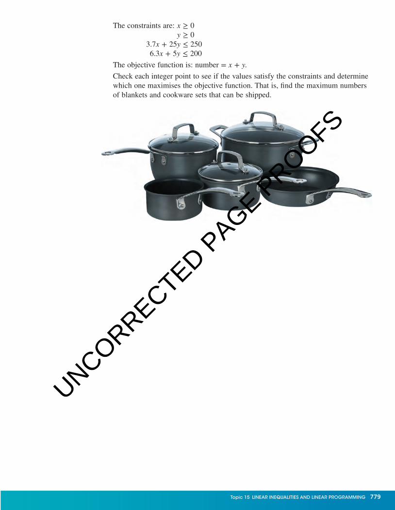
A manufacturer makes two products — blankets and cookware sets — that need to be shipped in special containers. Each blanket weighs 3.7 kg and has a volume of 6300 cm3. Each cookware set weighs 25 kg and has a volume of 5000 cm3. The shipping containers can hold 250 kg and have a maximum volume of 200 000 cm3. Use linear programming techniques to determine the largest number of each item that can be shipped in one container for optimal efficiency.

The decision variables are: let x = number of blankets shippedlet y = number of cookware sets shipped.

The constraints are: x ≥ 0y ≥ 0

3.7x + 25y ≤ 250 6300x + 5000y ≤ 200 000 or 6.3x + 5y ≤ 200 (dividing by 1000)

The solution region is shown in the diagram.

The vertices are found as follows. The intersection of the two lines shown (Point B) is found by solving the simultaneous linear equations:

3.7x + 25y = 250 6.3x + 5y = 200

The solution is x = 26.98, y = 6.01.

The other vertices are (0, 10) and (31.7, 0).

The objective function, which we wish to maximise, is:

Objective function: number = x + y.

The values of the objective function are:

Point A: (0, 10); number = 10Point B: (26.9, 6.01); number = 32.91* *MaximumPoint C: (31.7, 0); number = 31.7

Note that the ‘optimal’ solution (26.9, 6.01) has non-integer values for x and y. How is it possible to ship 26.9 blankets and 6.01 cooking sets? This is a class of problem known as integer programming, which is beyond the scope of Further Mathematics; however, a possible solution is given as follows.

B

C

A

Region required

20y

x

10

10 20 30 400



UNCORRECTED PAGE P

ROOFS

10

10

5

0 20 30

y

x

Region required

A

B

C

Consider the integer points closest to the optimal solution: (27, 6) and its nearest 8 neighbours, (26, 7), (27, 7), (28, 7), ..., (28, 5).

Check each one in turn to see if they satisfy the constraints and choose the one that has the largest objective function value.

The completion of this problem is left as question 16 in Exercise 15.5.

Applications1 WE11 A gardener can buy grass blends from three suppliers: Greener Grass, Green

Lawns and Green Turf. In each case the grass contains a number of grasses; two of these are tall fescue and ryegrass. When combined, the grass can contain no more than 25% tall fescue and no more than 15% ryegrass. The gardener needs to use 2 tonnes of grass in total, by purchasing from each supplier. Each supplier contains the following amounts of tall fescue and ryegrass.

Tall fescue Ryegrass Cost per tonne

Greener Grass 20% 18% $100

Green Lawns 25% 12% $90

Green Turf 30% 16% $75

Maximum allowed 25% 15%

Use linear programming techniques (sliding line or corner point) to find the amount of grass to purchase from each supplier in order to keep costs to a minimum. That is:

a define the decision variablesb define the constraintsc graph the solution regiond define the objective functione determine the amount of grass purchased from each nursery.

2 A smoothie store buys orange juice from suppliers A, B and C. In each case the juice contains pulp and seeds. When combined, the juice must contain no more than 7% pulp and no more than 4% seeds. The owner wishes to purchase a total of 150 litres of juice from three suppliers. Each supplier’s juice contains the following amounts of pulp and seeds.

ExErCisE 15.5

PrACtisE



UNCORRECTED PAGE P

ROOFS

Pulp Seeds Cost per litre (c)

Supplier A 10% 4% 45

Supplier B 8% 6% 60

Supplier C 5% 3% 75

Maximum allowed 7% 4%

Use linear programming techniques (sliding line or corner point) to find the amount of juice to purchase from each supplier in order to keep costs to a minimum. That is:

a define the decision variablesb define the constraintsc graph the solution regiond define the objective functione determine the amount of juice purchased from each supplier.

3 WE12 Fast Grow nurseries grow plants at two nurseries and ship them to two different distributors.

Nursery A produces 750 plants; Nursery B produces 900 plants.

Distributor X wants 600 plants while Distributor Y wants 700 plants.

The shipping costs between nurseries (in dollars per plant) and distributors are shown in the following table.

Nursery A Nursery B

Distributor X $0.70 $0.80

Distributor Y $0.60 $0.65

Use linear programming techniques (sliding line or corner point) to determine the number of plants shipped between nurseries and distributors in order to minimise total shipping cost. That is:

a define the decision variables and summarise in a tableb define the constraints based on the fact that all shipments must be

non-negativec graph the solution regiond define the objective functione determine the best way to ship to minimise cost.

4 Digi Electronics produces digital radios at two factories and ships them to two different distributors. Each factory produces 27 radios per day.

Distributor X requires 23 radios while Distributor Y requires 19 radios.

The shipping costs (in dollars per radio) between the factories and the distributors are shown in the following table:

Factory A Factory B

Distributor X $7 $12

Distributor Y $5 $10

Use linear programming techniques (sliding line or corner point) to determine the number of radios shipped between factories and distributors in order to minimise total shipping cost. That is:



UNCORRECTED PAGE P

ROOFS

a define the decision variablesb define the constraints based on the fact that all shipments must be non-negativec graph the solution regiond define the objective functione determine the best way to ship to minimise cost.

5 A local restaurant owner buys his orange juice from three suppliers: A, B and C. In each case the juice contains unwanted pulp and seeds. When combined, the juice must contain no more than 5% pulp and no more than 3% seeds. The owner wishes to purchase a total of 100 litres of juice from among the three suppliers. Each supplier’s juice contains the following amounts of pulp and seeds:

Pulp Seeds Cost per litre (¢)

Supplier A 7% 5% 35

Supplier B 6% 3% 45

Supplier C 3% 2% 55

Maximum amount of contaminant allowed

5% 3%

Supplier A charges $0.35 per litre, supplier B charges $0.45 per litre and supplier C charges $0.55 per litre. Use linear programming methods to find the amount of juice to buy from each supplier in order to minimise the cost. That is:

a identify the decision variablesb define the constraint inequation caused by the restriction on pulpc define the constraint inequation caused by the restriction on seedsd define the remaining constraints.

6 Using the information provided and the answers calculated in question 5,

a graph the solution regionb define the objective functionc find the amount of juice purchased from each supplier.

7 A canner of fruit salad can buy from three different suppliers, A, B and C, subject to the following restrictions on the minimum amount of peaches and cherries in the salad.

Ingredient Cost per kg ($)Peaches Cherries

Supplier A 23% 5% 1.10

Supplier B 20% 3% 0.90

Supplier C 30% 7% 1.40

Minimum amount of ingredient allowed

22% 4%

ConsoliDAtE



UNCORRECTED PAGE P

ROOFS

Use linear programming techniques (sliding line or corner point) to find the amount of salad to buy from each supplier to make up a total of 100 kg with the minimum cost.

8 Kumquat Computers produces computers at its two factories and ships them to two distributors. Each factory produces 35 computers per day. Distributor X requires 30 computers; distributor Y requires 25. The shipping costs (in dollars per computer) between the factories and the distributors are shown in the table:

Factory 1 Factory 2



Use linear programming methods (sliding line or corner point) to find the number of computers shipped between factories and distributors in order to minimise the cost. That is:

a define the decision variablesb define the constraints based on the fact that all shipments must be non-negativec graph the solution regiond define the objective functione determine the best way to ship to minimise cost.

9 A manufacturer of refrigerators has two factories: the first produces 60 refrigerators per week, the second produces 25 per week. Their two distributors require 30 and 45 refrigerators respectively. The shipping costs (in dollars per refrigerator) are given in the following table.

Factory 1 Factory 2



Use linear programming techniques (sliding line or corner point) to determine the best way to ship to minimise cost.

10 A shoemaker has two factories which produce 50 and 80 dozen pairs each. These are shipped to two factory outlets, Outlet X and Outlet Y, which require 50 and 30 dozen pairs each respectively. The shipping costs (in dollars per dozen pairs) are given in the following table.

Factory 1 Factory 2

Outlet X $14 $11

Outlet Y $16 $8

Use linear programming techniques (sliding line or corner point) to determine the best way to ship to minimise cost.

The following information relates to question 11, 12 and 13.

A cereal retailer obtains a particular type of cereal from three different suppliers, P, Q and R, subject to the following restrictions on the amounts of sultanas and dried apricots.



UNCORRECTED PAGE P

ROOFS

Sultanas Apricots Cost per kg ($)

Supplier P 15% 12% 1.20

Supplier Q 19% 10% 0.90

Supplier R 12% 15% 1.10

Minimum amount of ingredient needed

14% 11%

The total amount of cereal required is 100 kg.

11 If x = the number of kilograms of cereal from Supplier P and

y = the number of kilograms of cereal from Supplier Q,

then the constraint inequality caused by the restriction on sultanas is:

A 15x + 12y ≤ 1.20 B 3x + 7y ≥ 200C 3x + 7y ≤ 200 D 3x + 5y ≥ 400E 3x + 5y ≤ 400

12 The inequality which is not a constraint for this situation is:

A 3x + 5y ≤ 400 B x ≥ 0C y ≥ 0 D x + y ≥ 100E x + y ≤ 100

13 The feasible region for this situation is:

A

28 4–7

1331–3

Region required

y

x

100

0 80 100662–3

B

80

100

1000 x

y

4–7

28

2–3

66

1331–3

Region required

C

80

100

0 x

y

2–3

66

4–7

28

1331–3

Region required

100

D

80

100

0 x

y

2–3

66

4–7

28

1331–3

Region required

100



UNCORRECTED PAGE P

ROOFS

E

80

100

1000 x

y

2–3

66

4–7

28

1331–3

Region required

14 The line shown below has the equation of the form 2y + 3x = 6c.

The value of c must therefore be:

A 2B 5C 6D –6E –5

15 A refinery gets its petrol from three oil wells. Each well provides oil with a certain amount of lead and iso-octane according to the following table. The blended product must contain a maximum of 3.5% lead and a minimum of 65% iso-octane.

Ingredient

Cost per litre ($)Lead Iso-octane

Oil well A 4% 70% 0.24

Oil well B 2% 60% 0.22

Oil well C 6% 80% 0.26

Amount of ingredient allowed

3.5% maximum

65% minimum

Use linear programming techniques (sliding line or corner point) to determine how much to buy, at minimum cost, from each well per 100 litres of petrol refined.

16 Refer back to the text example on pages 772–3, which illustrated a limitation of the linear programming techniques used in this topic. The optimal solution involved non-integers but the situation required integer solutions. The 9 integer points surrounding the optimal solution are shown in the diagram {(26, 7), (27, 7), (28, 7), ..., (28, 5)}.

15

5

10

50 x

y

10 15

MAstEr

10

10

5

0 20 30

y

x

Region requiredA

B

C



UNCORRECTED PAGE P

ROOFS

The constraints are: x ≥ 0y ≥ 0

3.7x + 25y ≤ 250 6.3x + 5y ≤ 200

The objective function is: number = x + y.

Check each integer point to see if the values satisfy the constraints and determine which one maximises the objective function. That is, find the maximum numbers of blankets and cookware sets that can be shipped.



UNCORRECTED PAGE P

ROOFS

ONLINE ONLY 15.6 Review www.jacplus.com.au

the Maths Quest review is available in a customisable format for you to demonstrate your knowledge of this topic.

the review contains:• Multiple-choice questions — providing you with the

opportunity to practise answering questions using CAS technology

• short-answer questions — providing you with the opportunity to demonstrate the skills you have developed to ef� ciently answer questions using the most appropriate methods

• Extended-response questions — providing you with the opportunity to practise exam-style questions.

A summary of the key points covered in this topic is also available as a digital document.

REVIEW QUESTIONSDownload the Review questions document from the links found in the Resources section of your eBookPLUS.

studyON is an interactive and highly visual online tool that helps you to clearly identify strengths and weaknesses prior to your exams. You can then con� dently target areas of greatest need, enabling you to achieve your best results.

ONLINE ONLY Activitiesto access eBookPlUs activities, log on to

www.jacplus.com.au

InteractivitiesA comprehensive set of relevant interactivities to bring dif� cult mathematical concepts to life can be found in the Resources section of your eBookPLUS.



UNCORRECTED PAGE P

ROOFS

15 AnswersUnless stated otherwise, for all graphical answers to topic 15, ▭ indicates the region required.

EXERCISE 15.21

10

5 4

–5

–10

5 7 10–5–10 0 x

y

2

10

5

–5

–10

5 10 13–5–10 0 x

y

3

10

5

–5

–10

5

12

–5–10 0 x

y

–7

10

4

10

5

–5

–10

5 10–5–10 0 x

y

–6 2–3

–4

5

10

5

–5

–10

5 10–5–10 0

y

x

6 a

10

5

–5

–10

5 10–5–10 0 x

y

b

10

5

–5

–10

5 10–5–10 0 x

y

c

10

5

–5

–10

5 10–5–10 0 x

y

d

20

10

–10

–20

10 20–10–20 0 x

y


c15LinearInequalitiesAndLinearProgramming.indd 781 12/09/15 8:33 PM

UNCORRECTED PAGE P

ROOFS

7

10

5

–5

–10

–10 5 10–5 0 x

y

8

10

5

–5

–10

5 10–10 0 x

y

–5

9

10

5

–5

–10

5 10–5–10 0 x

y

10

10

5

–5

–10

–10 5 10–5 x

y

0

11 B, E

12

10

5

–5

–10

5 10 15–5 0 x

y

13 C

14

10

5

–5

–10

5 10–5–10 0 x

y

15

10

5

–5

–10

5 10–5–10 0 x

y

16

30

15

–15

–30

5 10–5–10 0 x

y

ExErCisE 15.31

10

5

–4

–10

5

6

–5–10 0 x

y

10

–5

2

10

–5

–10

5

7

10–5

–3

–10 0 x

y12

5



UNCORRECTED PAGE P

ROOFS

3

5

–5

–10

5

6

89

10

12

–5–10 0 x

y

10

4

10

20

10

1215

5

0 20

y

x

25

5 15 25

24

5 3

1

2

10 x

y

2 3

6

10

20

10

15

5

0 20

y

x

25

5 15 25

7

10

5

–5

–10

5 10–5–10 0 x

y

8

10

5

–5

–10

5 10–5–10 0 x

y

9

10

5

–5

–10

5 10–5–10 0 x

y

10

10

–5

–10

5 10–5–10 0 x

y

5

11

8

5

3 70 x

y

12

8

4

0

y

x2 5

13 7

2

0

y

x3 5

14

3

1

0

y

x

6

2 6



UNCORRECTED PAGE P

ROOFS

15

7

3

10

0

y

x3 5 7

16

7

3

10

0

y

x3 5 7

17 D

18 a 2x + 2y ≥ 20, –x + y ≥ 5, x ≤ 15, y ≤ 15, x ≥ 0, y ≥ 0

b 20

1015

5

105 15 200 x

y

c (10, 10) does not lie in the solution region.

ExErCisE 15.41 a x = the number of 2-person cabins rented,

y = the number of 3-person cabins rented.

b 40x + 45y ≤ 3000

c 2x + 3y ≤ 180

2 x = amount invested in bonds, y = amount invested in real estate mortgages.

a x + y ≤ 1 000 000

b x ≥ 2y or x – 2y ≥ 0

3

80100

4060

20

(30, 40)

4020 60 80 1000 x

y

75 90

662–3

4 Total return = 0.06x + 0.11y

5 The club should rent 60 3-person cabins (and not rent any 2-person cabins).

6 The optimal ‘mix’ is to invest one-third in real estate (at 11%) and the rest in bonds (at 6%) in order to maximise return.

7 x = number of flat screen TVs, y = number of curved screen TVs

Objective function: Number = x + y

The company should make 15 000 flat screen TVs and 0 curved screen TVs.

8 Teacher A: 20x + 8y ≤ 320

Teacher B: 10x + 2y ≤ 100

10 text chapters and 0 tests

9 x = number of hours on football, y = number of hours on basketball

Objective function: Earnings = 6.5 x + 10 y

Kyle should play football for 20 hours and basketball for 10 hours to maximise his earnings at $230.

10 Staff to build the sofas: 9x + 8y ≤ 207

Shipping and packaging constraint: 2x + 5y ≤ 75

The optimal solution is when 15 leather and 9 cloth sofas are produced.

11 a x = number of model A made

y = number of model B made

b x ≥ 0, y ≥ 0, 5x + 18y ≤ 360, 5x + 4y ≤ 150

c 40

2030

10

2010 30 400 x

y

d Profit = 2.5x + 4y

e x = 18, y = 15, Profit = $105

12 a x = number of sedans sprayed

y = number of utilities sprayed

b x ≥ 0, y ≥ 0, 5x + 7y ≤ 140, 9x + 8y ≤ 183, 6x + 5y ≤ 120

13 a

10

20

1015

5

0 20

y

x

25

5 15 25

b Number = x + y

c x = 7, y = 15, Vehicles = 22

14 a x = models of monitor

y = models of disk drive

b x ≥ 0, y ≥ 0, 7x + 8y ≤ 320, 11x + 7y ≤ 319, 22x + 12y ≤ 594, 11x + 3y ≤ 264

15 a

10

40

2030

10

020

y

x

50

5

(21, 11)

(15, 22)

(8, 33)

15 25 30

b Profit = 150 000x + 120 000y

x = 8, y = 33, Profit = $5 160 000

16 The solution would be x = 0, y = 6, with a profit of $780.

17 x = number of apples

y = number of pieces of cheese

Constraints: x ≥ 0, y ≥ 0,

3x + 10y ≤ 98, 3x + 4y ≥ 50

Objective function:

Calorie intake = 100x + 85y



UNCORRECTED PAGE P

ROOFS

Solution: x = 6, y = 8, Calories = 1280

(6, 8)

15

5

10

100 x

y

20 30

18 x = indoor paint

y = outdoor paint

Constraints: x ≥ 0, y ≥ 0, 3x + 8y ≤ 100, x + y ≥ 30

Objective function:

Profit = 2.50x + 3.25y

Solution: x = 33.33, y = 0, Profit = $83.33

10

10

15

5

020

y

x5 15 25 30 35

(28, 2)

19 x = number of roses

y = number of tulips

Constraints: x ≥ 0, y ≥ 0, x + y ≤ 3000, x ≤ 3y, x ≥ 2y

Objective function: Income = 15x + 6y

Solution: x = 2250, y = 750,

Income = $38 250

2000

3000

1000

1000 2000 3000

(3000, 1500)

(3000, 1000)

(2250, 750)

(2000, 1000)

0

CA

B

x

y

20 x = value of shares

y = value of gold

Constraints: x ≥ 0, y ≥ 0, x + y ≤ 100 000, x – 2y ≤ 0, x – 0.5y ≥ 0

Objective function:

Profit = 0.1x + 0.16y

Solution: x = 33 333.33,

y = 66 666.67, profit = $14 000

80100

4060

20

(× $1000)

(× $

1000

)

(33, 66)

4020 60 80 1000 x

y

(33, 66)(66, 33)

21 C

22 a x + y ≤ 50

12 000x + 12 500y ≤ 490 000

y ≥ x

x ≥ 0

y ≥ 0

b OC is y ≥ x

BF is x + y ≤ 50

AE is 12 000x + 12 500y ≤ 490 000

c C (25, 25)

D (20, 20)

d 20 sedans and 20 wagons

ExErCisE 15.51 a Let x = tonnes of grass from Greener Grass

Let y = tonnes of grass from Green Lawns

Let (2 − x − y)= tonnes of grass from Green Turf

b 10x + 5y ≥ 10, 4y − 2x ≥ 2, x ≥ 0, y ≥ 0, 2 − x − y ≥ 0 or x + y ≤ 2

c

1.62.0

0.81.2

0.4

0.80.4 1.2 1.6 2.00

A

BC

x

y

Point A: (0, 2), Point B: a35, 4

5b, Point C: (1, 1)

d Cost = 25x + 15y + 150

e 35 of a tonne from Greener Grass, 4

5 of a tonne from

Green Lawns, 35 of a tonne from Green Turf

2 a x = litres of orange juice from Supplier A

y = litres of orange juice from Supplier B

(150 − x − y) = litres of orange juice from Supplier C

b 5x + 3y ≤ 300, x + 3y ≤ 150, x ≥ 0, y ≥ 0, 150 − x − y ≥ 0 or x + y ≤ 150

c

80100120140160

4060

20

4020 60 80 100

120

140

1600

AB

Cx

y

Point A: (0, 50)

Point B: (37.5, 37.5)

Point C: (60, 0)

d Cost = 11 250 − 30x − 15y

e 60 litres from Supplier A

0 litres from Supplier B

90 litres from Supplier C



UNCORRECTED PAGE P

ROOFS

3 a Nursery A Nursery B Total

Distributor X x (600 – x) 600

Distributor Y y (700 – y) 700

Total 750 900

b x ≥ 0

y ≥ 0

600 − x ≥ 0 or x ≤ 600

700 − y ≥ 0 or y ≤ 700

Nursery A: x + y ≤ 750

Nursery B: x + y ≥ 400

c

400

600

800

200

200 400 600 8000

A

B C

D

Ex

y

Point A: (0, 400)

Point B: (0, 700)

Point C: (50, 700)

Point D: (600, 150)

Point E: (600, 0)

Point F: (400, 0)

d Total cost = 935 − 0.1x − 0.05y

e Minimum cost is at Point D

Ship 600 from nursery A to distributor X

Ship 150 from nursery A to distributor Y

Ship 0 from nursery B to distributor X

Ship 550 from nursery B to distributor Y

4 a Factory A Factory B Total

Distributor X x (23 – x) 23

Distributor Y y (19 – y) 19

Total 27 27

b x ≥ 0

y ≥ 0

23 − x ≥ 0 or x ≤ 23

19 − y ≥ 0 or y ≤ 19

Factory A: x + y ≤ 27

Factory B:x + y ≥ 15

c

20

30

10

10 20 300

C

AB

D

F E x

y

Point A: (0, 15)

Point B: (0, 19)

Point C: (8, 19)

Point D: (23, 4)

Point E: (23, 0)

Point F: (15, 0)

d Total cost = 466 − 5x − 5y

e Minimum cost is at Point C or D: (8, 19) or (23, 4).

Ship 8 or 23 from factory A to distributor X

Ship 19 or 4 from factory A to distributor Y

Ship 15 or 0 from factory B to distributor X

Ship 0 or 15 from factory B to distributor Y

5 a x = litres purchased from supplier A

y = litres purchased from supplier B

100 – x – y = litres purchased from supplier C

b 4x + 3y ≤ 200

c 3x + y ≤ 100

d x ≥ 0, y ≥ 0, x + y ≤ 100

6 a

80100

4060

20

(20, 40)

(× $1000)

4020 60 80 1000 x

y

b Cost = −20x – 10y + 5500 (in cents)

c x = 20, y = 40. Cost = $47.00. Purchase 20 litres from A, 40 litres from each of B and C.

7 x = kg purchased from supplier A

y = kg purchased from supplier B

100 – x – y = kg purchased from supplier C

Constraints: 7x + 10y ≤ 800, 2x + 4y ≤ 300, x ≥ 0, y ≥ 0, x + y ≤ 100

80100

0 x

y

100 150

(25, 62.5)

(66.7, 33.3)



UNCORRECTED PAGE P

ROOFS

Objective function:

Cost = –0.3x – 0.5y + 140

x = 25, y = 62.5, Cost = $101.25

Purchase 25 kg from A, 62.5 kg from B and 12.5 kg from C

8 a x = computers from factory 1 to distributor X

y = computers from factory 1 to distributor Y

(30 – x) = computers from factory 2 to distributor X

(25 – y) = computers from factory 2 to distributor Y

b x ≥ 0, y ≥ 0, x ≤ 30, y ≤ 25, x + y ≤ 35, x + y ≥ 20

c

2025

35

200 x

y

30 35

d Cost = –30x – 15y + 2525

e x = 30, y = 5, Cost = $1550

Ship 30 from factory 1 to distributor X, 5 from factory 1 to distributor Y, 20 from factory 2 to distributor Y.

9 Variables:

x = refrigerators from factory 1 to distributor X

y = refrigerators from factory 1 to distributor Y

(30 – x) = refrigerators from factory 2 to distributor X

(45 – y) = refrigerators from factory 2 to distributor Y

455060

300 x

y

50 60

x ≥ 0, y ≥ 0, x ≤ 30, y ≤ 45,

x + y ≤ 60, x + y ≥ 50

Cost = –6x – 7y + 1935

x = 15, y = 45, Cost = $1530

Ship 15 from factory 1 to distributor X, 45 from factory 1 to distributor Y, 15 from factory 2 to distributor X.

10 Variables:

x = dozen pairs of shoes from factory 1 to distributor X

y = dozen pairs of shoes from factory 1 to distributor Y

(50 – x) = dozen pairs of shoes from factory 2 to distributor X

30

50

0 x

y

50

(30 – y) = dozen pairs of shoes from factory 2 to distributor Y x ≥ 0, y ≥ 0, x ≤ 50, y ≤ 30, x + y ≤ 50, x + y ≥ 0

Cost = 3x + 8y + 790 x = 0, y = 0.

Cost = $790 Ship 50 from factory 2 to distributor X, 30 from factory 2 to distributor Y.

11 B

12 D

13 D

14 B

15 x = litres purchased from supplier A

y = litres purchased from supplier B

100 – x – y = litres purchased from supplier C

Constraints: 2x + 4y ≥ 250,

x + 2y ≤ 150, x ≥ 0, y ≥ 0,

x + y ≤ 100

10075

62.5

1000 x

y

150

125

(50, 50)

(75, 25)

Objective function:

Cost = –0.02x – 0.04y + 26

x = 0, y = 75. Cost = $23

x = 50, y = 50. Cost = $23

Purchase 75 L from B and 25 L from C (none from A) or purchase 50 L from A and 50 L from B (none from C)

16 Feasible solutions are (26, 5), (27, 5), (26, 6). Choose either of the last 2 points (x + y = 32).

The maximum number of Blankets and cookware sets that can be shipped is 32.



UNCORRECTED PAGE P

ROOFS

Documents

PAGE PROOFS Linear inequalities programming and linear · PDF fileLinear inequalities To begin our work in linear programming, we fi rst have to develop some skills with linear inequalities