Embed Size (px)
Citation preview

Karlstads universitet 651 88 KarlstadT fn 054-700 10 00 Fax 054-700 14 60
[email protected] www.kau.se
Computer science
Jonas Brolin
Mikael Hedegren
Packet Aggregation in Linux
Computer science
C-level thesis 15p
Date/Term: 08-06-03
Supervisor: Andreas Kassler
Examiner: Martin Blom
Serial Number: C2008:04

ii
This report is submitted in partial fulfillment of the requirements for the
Bachelor’s degree in Computer Science. All material in this report which is
not my own work has been identified and no material is included for which
a degree has previously been conferred.
Jonas Brolin
Mikael Hedegren
Approved 2008 06 03
Advisor: Andreas Kassler
Examiner: Martin Blom
iii
Abstract
Voice over IP (VoIP) traffic in a multi-hop wireless mesh network (WMN) suffers from a
large overhead due to mac/IP/UDP/RTP headers and time collisions. A consequence of the
large overhead is that only a small number of concurrent VoIP calls can be supported in a
WMN[17]. Hop-to-hop packet aggregation can reduce network overhead and increase the
capacity. Packet aggregation is a concept which combines several small packets, destined to a
common next-hop destination, to one large packet. The goal of this thesis was to implement
packet aggregation on a Linux distribution and to increase the number of concurrent VoIP
calls. We use as testbed a two-hop WMN with a fixed data rate of 2Mbit/s. Traffic was
generated between nodes using MGEN[20] to simulate VoIP behavior. The results from the
tests show that the number of supported concurrent flows in the testbed is increased by 135%
compared to unaggregated traffic.
iv
Contents
1 Introduction....................................................................................................................1
1.1 Primary goals.......................................................................................................1
1.2 Secondary goals...................................................................................................1
1.3 Outline..................................................................................................................2
2 Background.....................................................................................................................3
2.1 Introduction..........................................................................................................3
2.2 Packet Aggregation..............................................................................................3
2.3 Linux Networking................................................................................................5 2.3.1 Introduction 2.3.2 Linux Networking stack 2.3.3 Socket buffers 2.3.4 Introduction to Linux Traffic Control 2.3.5 Netfilter
2.4 Ad hoc On-Demand Distance Vector (AODV)...................................................17 2.4.1 AODV-UU
2.5 OpenWrt on Linksys ..........................................................................................19 2.5.1 The Linksys WRT54GL version 1.1 2.5.2 OpenWrt
2.6 Summary..............................................................................................................20
3 Implementation...............................................................................................................21
3.1 Introduction..........................................................................................................21
3.2 Different approaches to packet aggregation.........................................................21 3.2.1 Implementation as a user space application 3.2.2 Implementation as a kernel module 3.2.3 Implementation directly in networking stack 3.2.4 Conclusions
3.3 Implementation ...................................................................................................24 3.3.1 Packet Layout 3.3.2 Qdisc sch_simplerr (Classifier Module) 3.3.3 Qdisc sch_aggregate (Aggregation Module) 3.3.3.1 About maxSize, agg_max_size, -max and dynamic marking 3.3.4 deaggregate (Deaggregation Module) 3.3.5 Installation and configuration
3.4 AODV Extension.................................................................................................39 3.4.1 Calculating Signal-to-Noise Ratio (SNR) 3.4.2 Calculating Smoothed SNR 3.4.2 Retrieving signal and noise power
v
3.4.3 Extending AODV-UU 3.4.4 AODV Extension Issues 3.4.5 AODV Extension – Conclusion
3.5 OpenWRT............................................................................................................44
3.6 Summary..............................................................................................................45
4 Test and Evaluation........................................................................................................47
4.1 Introduction..........................................................................................................47
4.2 Test Setup ............................................................................................................48
4.3 Results..................................................................................................................50 4.3.1 Network test results. 4.3.2 Results from the aggregation module
4.4 Summary..............................................................................................................62
5 Conclusions......................................................................................................................63
5.1 General Summary.................................................................................................63
5.2 Open Issues..........................................................................................................63
5.3 Future Work.........................................................................................................65
5.4 Other Applications...............................................................................................65
5.5 Summary and Conclusions...................................................................................66
References...........................................................................................................................67
vi
List of Figures
Figure 1: Overview of Linux network stack with Netfilter hooks and modules described in the thesis...........................................................................................................................6
Figure 2: NAPI-aware drivers versus non-NAPI-aware devices [3]...............................7
Figure 3: Simple representation of the socket buffer memory map...............................11
Figure 4: Qdisc tree [26]......................................................................................................12
Figure 5: classes, filters and qdiscs.....................................................................................13
Figure 6: FIFO qdisc illustration.......................................................................................13
Figure 7: Example of AODV route discovery (picture from [1])....................................18
Figure 8: Construction and deconstruction of a meta packet.........................................24
Figure 9: qdisc organization..............................................................................................25
Figure 10: Dequeue flowchart............................................................................................27
Figure 11: Aggregation queue struct.................................................................................31
Figure 12: The mark field...................................................................................................33
Figure 13: AODV link measurement.................................................................................39
Figure 14: Test setup...........................................................................................................48
vii
List of graphs
Graph 1: Application throughput with 1 and 2Mbit bit rate..........................................50
Graph 2: End to end Latency in low traffic and total test run. ......................................52
Graph 3: Average loss ratio over the first 175s.................................................................53
Graph 4: Average jitter as measured by TRPR................................................................54
Graph 5: Supported flows in the testbed...........................................................................55
Graph 6: Latency over time with 4, 24, 48, 52 and 68 injected flows.............................58
Graph 7: Aggregation ratio................................................................................................61
Graph 8: Average packets sent per flow............................................................................61
viii
1 Introduction
This thesis describes the implementation of an aggregation scheme for small packets over
wireless links in order to increase performance of Voice over IP in wireless mesh networks.
The scheme was first introduced by in [1] and tested in the NS2 network emulator with
promising results.
1.1 Primary goals
The primary goals of this project was to implement aggregation and deaggregation in a
common Linux environment, to provide means to configuring and installing the new modules,
to perform a basic test as a proof of concept.
Similar projects have implemented packet aggregation in hardware, [24] and [25].
However the goal of this project was to implement aggregation in a common Linux
environment for more flexible use.
1.2 Secondary goals
The secondary goals of this project consists of implementing a full dynamic aggregation
scheme on a commonly available routing platform. The platform in question is the Linksys
WRT54GL with OpenWrt Linux based firmware. To facilitate the dynamic link aware
aggregation, extensions to the Advanced On Demand Routing protocol as presented by in [1]
was also needed.
1
1.3 Outline
● Background information about concepts and ideas used in this project are presented
in chapter 2.
● Implementation is described in chapter 3.
● The test results are shown in chapter 4.
● Conclusions from the tests and the project as a whole are presented in chapter 5.
2
2 Background
2.1 Introduction
This chapter introduces necessary background information on the components later used in
the implementation. Section 2.2 introduces the concept of packet aggregation as presented by
[1]. Section 2.3 presents the parts of Linux Networking that are relevant to this thesis, mainly
the kernel portion. The concepts presented within section 2.3 include the Linux network stack,
socket buffers, traffic control and Netfilter, found in section 2.3.2, 2.3.3, 2.3.4 and 2.3.5,
respectively. In section 2.4 the routing protocol AODV is presented. Information about the
customizable Linux-based router firmware OpenWRT can be found in section 2.5.
2.2 Packet Aggregation
The objective of this project is to implement packet aggregation, as presented by in [1], in
a common Linux environment, install and evaluate the components on a cheap commonly
available routing platform, in this case the Linksys WRT54GL.
To fully understand the rest of this essay it is vital that one understands the concept of and
rationale behind packet aggregation. For a complete understanding of the subject we
recommend reading [1]. But for the propose of this document a digested introduction of
packet aggregation will suffice.
The idea behind Packet aggregation is to enhance performance of time critical applications
such as voice over IP (VoIP) over wireless mesh networks by reducing the mac traffic
contention and collision overhead. The mac layer overhead in wireless mesh networks is
primarily a result of the Carrier Sense Multiple Access / Collision Avoidance, or CSMA/CA
for short, approach to traffic contention on the medium, which, in case of VoIP, can amount
to a significant part of the total sending time for a packet. Overhead as high as 80% is
3
possible [1], in part because only the actual data traffic on the net is transmitted at the highest
speed possible. All other traffic (such as channel negotiation) is done at basic rate of 6 Mbit in
54 Mbit networks. By aggregating more packets into one meta packet and sending this packet
over the medium, the impact of the traffic contention overhead is reduced. Simulation in ns2
have shown promising results for this approach [1].
There are a few approaches to packet aggregation with respect to where the actual
aggregation will take place. Ranging from endpoint to endpoint, where the aggregation of
packets is performed at the originating host, and deaggregation is performed on the receiving
host, to link level aggregation where the aggregation and deaggregation of packets is
performed by every router on a hop-by-hop basis.
The discussion on the best approach for packet aggregation is a bit outside the scope of this
paper, since this paper is primarily concerned with the implementation of the approach
suggested in [1] but the main arguments for a link level approach is the ability to aggregate
several flows, and adapting the size of the meta packet according to the optimal frame size for
the particular link.
The scheme proposed by [1] is a forced delay approach where packets are delayed to wait
for additional packets to be sent to the same next-hop node, which are then aggregated and
sent with the first packet. Should the total size of packets to be sent reach the optimal frame
size within the delay time they will be aggregated and sent at once. If however no more
packets are to be sent to the next-hop node the original packet will be sent as is.
This approach requires a way to keep track of which packets are eligible for aggregation,
the next-hop nodes, the associated frame sizes and time.
A more thorough explanation of the packet aggregation algorithm is explained in section
3.3.3.
4
2.3 Linux Networking
2.3.1 Introduction
This section will introduce the Linux kernel networking stack in 2.3.2. After the general
network stack comes a presentation of the socket buffer, which is a very important data
structure in this thesis. Socket buffers are introduced in section 2.3.3. Section 2.3.4 outlines
Linux traffic control. In the last section there is a presentation of the netfilter, which is a part
of the Linux iptables firewall and is later used in the implementation.
2.3.2 Linux Networking stack
This introduction to the Linux network stack presents the kernel handling of network
packets from the reception on the incoming device via routing or user space handling to
leaving on the outgoing device. As this section is intended as background information for the
rest of the thesis, only information about the specific parts on which the implementation
depends are discussed in detail and other parts will mentioned but a deeper discussion of these
parts is considered outside of the scope of this thesis. Some parts of Linux networking, such
as socket buffers, traffic control and netfilter are discussed separately in 2.3.3, 2.3.4 and 2.3.5.
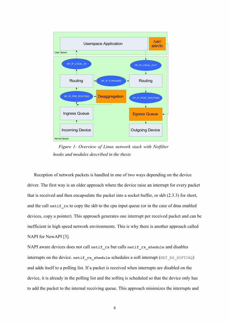
Figure 1 illustrates the Linux network stack including Netfilter hooks (ovals) and where
traffic control, aggregation (in Egress queue) and deaggregation is placed.
5
Reception of network packets is handled in one of two ways depending on the device
driver. The first way is an older approach where the device raise an interrupt for every packet
that is received and then encapsulate the packet into a socket buffer, or skb (2.3.3) for short,
and the call netif_rx to copy the skb to the cpu input queue (or in the case of dma enabled
devices, copy a pointer). This approach generates one interrupt per received packet and can be
inefficient in high speed network environments. This is why there is another approach called
NAPI for NewAPI [3].
NAPI aware devices does not call netif_rx but calls netif_rx_shedule and disables
interrupts on the device. netif_rx_shedule schedules a soft interrupt (NET_RX_SOFTIRQ)
and adds itself to a polling list. If a packet is received when interrupts are disabled on the
device, it is already in the polling list and the softirq is scheduled so that the device only has
to add the packet to the internal receiving queue. This approach minimizes the interrupts and
6
Figure 1: Overview of Linux network stack with Netfilter
hooks and modules described in the thesis
User Space
Kernel Space
Incoming Device
Ingress Queue
Routing
Outgoing Device
Egress Queue
Userspace Application
Routing
NF_IP_LOCAL_INNF_IP_LOCAL_OUT
NF_IP_PRE_ROUTING
NF_IP_FORWARD
NF_IP_POST_ROUTING
/usr/sbin/tc
Deaggregation
the processor(s) can process incoming packets at a rate that it can manage and schedule
network processing fairly compared to other kernel tasks.
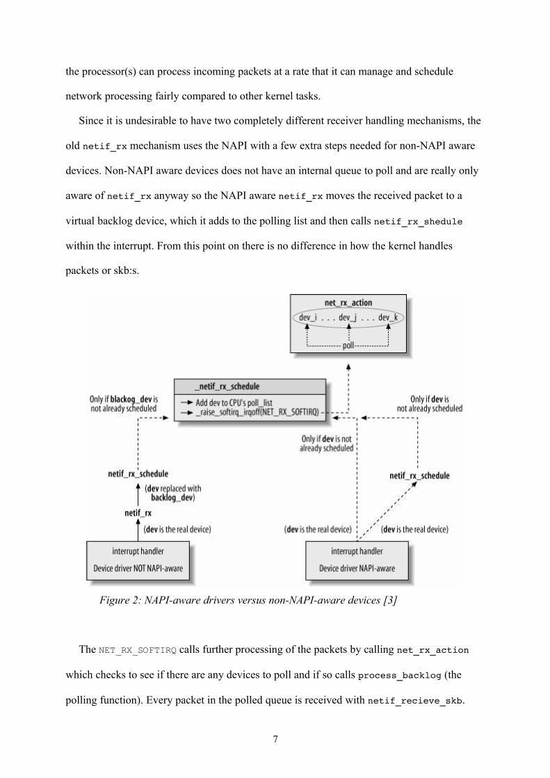
Since it is undesirable to have two completely different receiver handling mechanisms, the
old netif_rx mechanism uses the NAPI with a few extra steps needed for non-NAPI aware
devices. Non-NAPI aware devices does not have an internal queue to poll and are really only
aware of netif_rx anyway so the NAPI aware netif_rx moves the received packet to a
virtual backlog device, which it adds to the polling list and then calls netif_rx_shedule
within the interrupt. From this point on there is no difference in how the kernel handles
packets or skb:s.
The NET_RX_SOFTIRQ calls further processing of the packets by calling net_rx_action
which checks to see if there are any devices to poll and if so calls process_backlog (the
polling function). Every packet in the polled queue is received with netif_recieve_skb.
7
Figure 2: NAPI-aware drivers versus non-NAPI-aware devices [3]
This function moves the skb from layer 2 to layer 3, which includes setting the pointers to the
level 3 headers and possibly dropping or bridging it, depending on kernel configuration and
policies in place.
The actual passing to level 3 is done by calling IP_rcv, in case of IP v4 .This function is
responsible for some basic sanity checks such as checksum and length. Just before the
function finishes it will invoke any function registered with the first netfilter hook.
(NF_PRE_ROUTE). If the skb is not dropped or consumed by the netfilter hook then
IP_rcv_finnish is called. This function decides whether the packet should be forwarded or
delivered locally. If the packet is delivered locally, then IP_local_deliver will do transport
sanity checks and initiate transport header pointers and invoke functions registered to the
second netfilter hook. IP_local_deliver_finish will decide based on the IP protocol field
which protocol handler should handle the packet for delivery to user space sockets or internal
kernel processing (such as with ICMP).
Level 4 handling is outside the scope of this thesis and will not be discussed in any more
detail in this section.
If the skb is destined for another host then it is forwarded with ip_forward that performs
the basic sanity checks and invokes the third netfilter hook(NF_IP_FORWARD) before calling
ip_forward_finish which does the actual routing, i.e. decides what outgoing device to send
the skb to.
Routing is finished with the call to IP_output and IP_output_finish.
IP_output_finish calls the last netfilter hook (NF_IP_POST_ROUTING) before calling
IP_output_finish2.
Sending an skb to a device for transmission is done with a call to dev_queue_xmit which
enqueues the skb to the traffic control queue that is bonded to the device (Qdisc). If the device
is ready to send the dequeue function in the queue is called and the frame is sent by the
device.
8

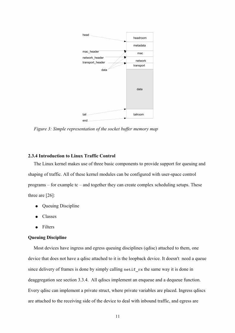
2.3.3 Socket buffers
The Linux networking stack is primarily concerned with the manipulation of socket buffers
which is a data type described in sk_buff.h found in the /include/linux directory in the
Linux source code.
The socket buffer, or skb as it is commonly known, is a complex data type which has
undergone some fairly major changes in the course of the Linux kernel development, but its
purpose has remained the same, namely to hold information of network packets. A full
presentation of all the fields and operations of the skb would take up too much space and is
outside the scope of this essay but a quick introduction of the structure, some of its data fields
and operations is vital to the understanding of this essay and some of our design decisions.
An skb contains a header and data, shown in figure 3. The header contains metadata fields
which are of primary concern to the kernel and handling of the packet. There are some cases
in which an skb is directly manipulated by a user space program. But these are special cases.
One of those will be discussed later in the presentation of different approaches to
implementation (see 3.2).
The primary fields of interest in this essay are next and prev, dev, dst, cb, len,
data_len, mark, transport_header, network_header, mac_header, tail, end,
head and data.
● prev: The prev and next pointers are pointers to the other nodes in a doubly liked
list. An skb is always part of a list in the kernel [3]. This list manipulation is largely
what qdiscs do.
● dev: The dev pointer is a pointer to the device that the skb arrived on or is leaving
on.
● dst: The dst pointer is a pointer to a dst_entry struct [/net/dst.h]. It holds
information about the destination of the packet and is manipulated by the routing
module in the kernel. This particular struct can be cast to an rtable struct
9
[/net/route.h] (which is done in the routing module) and this cast gives easy access
to all routing information regarding this packet.
● cb: The cb field is a 48 byte field which is free to use for private variables and will
not survive between layers in the networking stack.
● length: The length fields differ somewhat in what they represent, len is the length
of data including headers and will differ between layers in the network stack, i.e. in
layer 3 it will include the transport and network header but not the mac header.
data_len is the length of the actual data that is sent via the socket.
● mark: The mark field is an unsigned 32 bit integer which can be set by iptables or
any application capable of manipulating the skb directly. It is used in this
implementation to separate traffic and pass on information about frame size.
● transport_header, network_header and mac_header: The
transport_header, network_header and mac_header fields are pointers to the
respective header within the data part of the skb. Usage of the pointers are not defined
in layers above that correspond to the header, so for instance the mac_header is not
defined outside of the network devices. The data pointer points to the start of the
current level header, or active data. As the packet moves between levels, the data
pointer is moved to the appropriate header, e.g. when a packet is received on a device
and passed to the kernel for IP handling then the data pointer is simply moved from
the mac_header to the network_header. This saves cpu cycles compared to deleting
the MAC header.
● head, tail and end: The head, tail and end pointers exist for memory
management. This introduces the terms head room and tail room which are used to
determine if there is enough space to insert data at the beginning or end of the skb.
10
2.3.4 Introduction to Linux Traffic Control
The Linux kernel makes use of three basic components to provide support for queuing and
shaping of traffic. All of these kernel modules can be configured with user-space control
programs – for example tc – and together they can create complex scheduling setups. These
three are [26]:
● Queuing Discipline
● Classes
● Filters
Queuing Discipline
Most devices have ingress and egress queuing disciplines (qdisc) attached to them, one
device that does not have a qdisc attached to it is the loopback device. It doesn't need a queue
since delivery of frames is done by simply calling netif_rx the same way it is done in
deaggregation see section 3.3.4. All qdiscs implement an enqueue and a dequeue function.
Every qdisc can implement a private struct, where private variables are placed. Ingress qdiscs
are attached to the receiving side of the device to deal with inbound traffic, and egress are
11
Figure 3: Simple representation of the socket buffer memory map
data
transport
network
mac
metadata
head
data
tail
end
network_header
mac_header
transport_header
headroom
tailroom
mounted on the sending side to deal with outbound traffic. These will both be discussed later
in this chapter.
Qdisc Classes
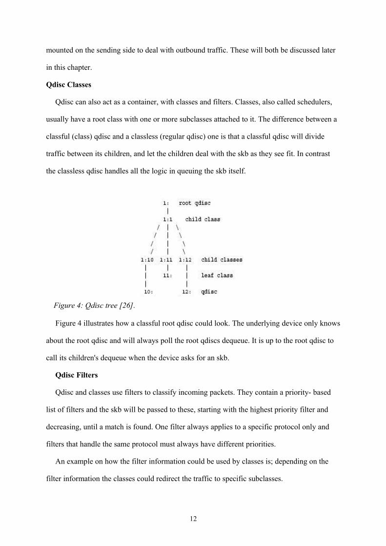
Qdisc can also act as a container, with classes and filters. Classes, also called schedulers,
usually have a root class with one or more subclasses attached to it. The difference between a
classful (class) qdisc and a classless (regular qdisc) one is that a classful qdisc will divide
traffic between its children, and let the children deal with the skb as they see fit. In contrast
the classless qdisc handles all the logic in queuing the skb itself.
Figure 4 illustrates how a classful root qdisc could look. The underlying device only knows
about the root qdisc and will always poll the root qdiscs dequeue. It is up to the root qdisc to
call its children's dequeue when the device asks for an skb.
Qdisc Filters
Qdisc and classes use filters to classify incoming packets. They contain a priority- based
list of filters and the skb will be passed to these, starting with the highest priority filter and
decreasing, until a match is found. One filter always applies to a specific protocol only and
filters that handle the same protocol must always have different priorities.
An example on how the filter information could be used by classes is; depending on the
filter information the classes could redirect the traffic to specific subclasses.
12
Figure 4: Qdisc tree [26].
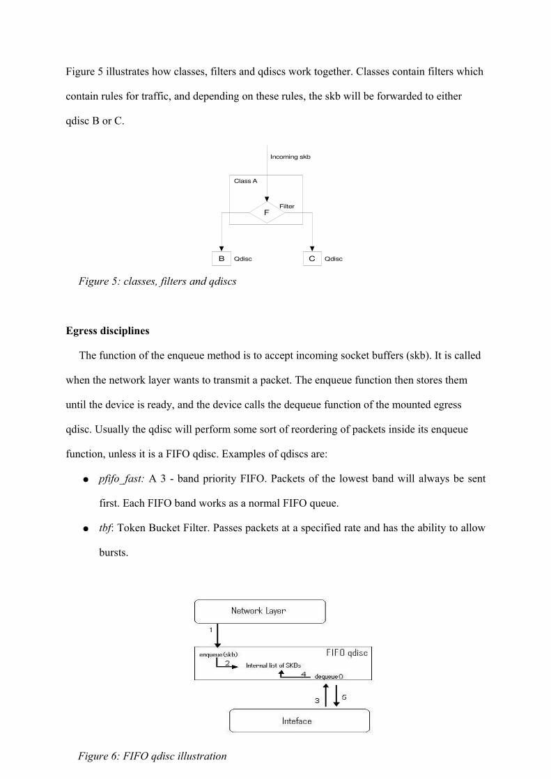
Figure 5 illustrates how classes, filters and qdiscs work together. Classes contain filters which
contain rules for traffic, and depending on these rules, the skb will be forwarded to either
qdisc B or C.
Egress disciplines
The function of the enqueue method is to accept incoming socket buffers (skb). It is called
when the network layer wants to transmit a packet. The enqueue function then stores them
until the device is ready, and the device calls the dequeue function of the mounted egress
qdisc. Usually the qdisc will perform some sort of reordering of packets inside its enqueue
function, unless it is a FIFO qdisc. Examples of qdiscs are:
● pfifo_fast: A 3 - band priority FIFO. Packets of the lowest band will always be sent
first. Each FIFO band works as a normal FIFO queue.
● tbf: Token Bucket Filter. Passes packets at a specified rate and has the ability to allow
bursts.
13
Figure 5: classes, filters and qdiscs
B C
Class A
QdiscQdisc
void enqueue(skb){int x = filter(skb)if(x==1) b.enqueue(skb);else if(x==2) c.enqueue(skb);}
C QdiscB Qdisc
A Class
F
Filter
C QdiscB Qdisc
Class A
FFilter
Incoming skb
Figure 6: FIFO qdisc illustration
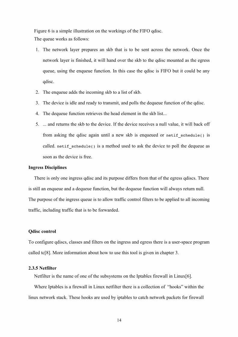
Figure 6 is a simple illustration on the workings of the FIFO qdisc.
The queue works as follows:
1. The network layer prepares an skb that is to be sent across the network. Once the
network layer is finished, it will hand over the skb to the qdisc mounted as the egress
queue, using the enqueue function. In this case the qdisc is FIFO but it could be any
qdisc.
2. The enqueue adds the incoming skb to a list of skb.
3. The device is idle and ready to transmit, and polls the dequeue function of the qdisc.
4. The dequeue function retrieves the head element in the skb list...
5. ... and returns the skb to the device. If the device receives a null value, it will back off
from asking the qdisc again until a new skb is enqueued or netif_schedule() is
called. netif_schedule() is a method used to ask the device to poll the dequeue as
soon as the device is free.
Ingress Disciplines
There is only one ingress qdisc and its purpose differs from that of the egress qdiscs. There
is still an enqueue and a dequeue function, but the dequeue function will always return null.
The purpose of the ingress queue is to allow traffic control filters to be applied to all incoming
traffic, including traffic that is to be forwarded.
Qdisc control
To configure qdiscs, classes and filters on the ingress and egress there is a user-space program
called tc[8]. More information about how to use this tool is given in chapter 3.
2.3.5 Netfilter
Netfilter is the name of one of the subsystems on the Iptables firewall in Linux[6].
Where Iptables is a firewall in Linux netfilter there is a collection of “hooks” within the
linux network stack. These hooks are used by iptables to catch network packets for firewall
14
processing. The netfilter hooks can be used not only by the firewall but by any application
that registers a kernel mode function with one or more of them. E.g. AODV-UU uses one
netfilter hook.
Some of the netfilter hooks are presented in 2.3.2 and the locations are illustrated in the
figure 1 in the same chapter. A table of the hooks and return types is presented at the end of
the chapter.
The mechanism of these hooks is quite simple; at different places in the network code, a
netfilter invocation code is called. This code calls all functions registered with this hook in
order of priority. Once a function finishes and returns a value the code will call the next
function if the return value is NF_ACCEPT, otherwise it will free its reference to the packet,
or skb, and update statistics according to the return code.
To register a function with a hook a few things has to be taken into account.
First, the function call has to conform to the format defined in the netfilter header file, it
has to be present in the kernel, either directly or as a part of a kernel module. It is however
perfectly possible to forward an skb directly to user space for processing.
Second, a netfilter hook struct has to be initialized with the proper hook number, priority
and function pointer to the function in question. This struct is initialized as part of the module
initialization process.
Once these requirements are met the function is registered to the desired netfilter hook as
soon as the module is initialized.
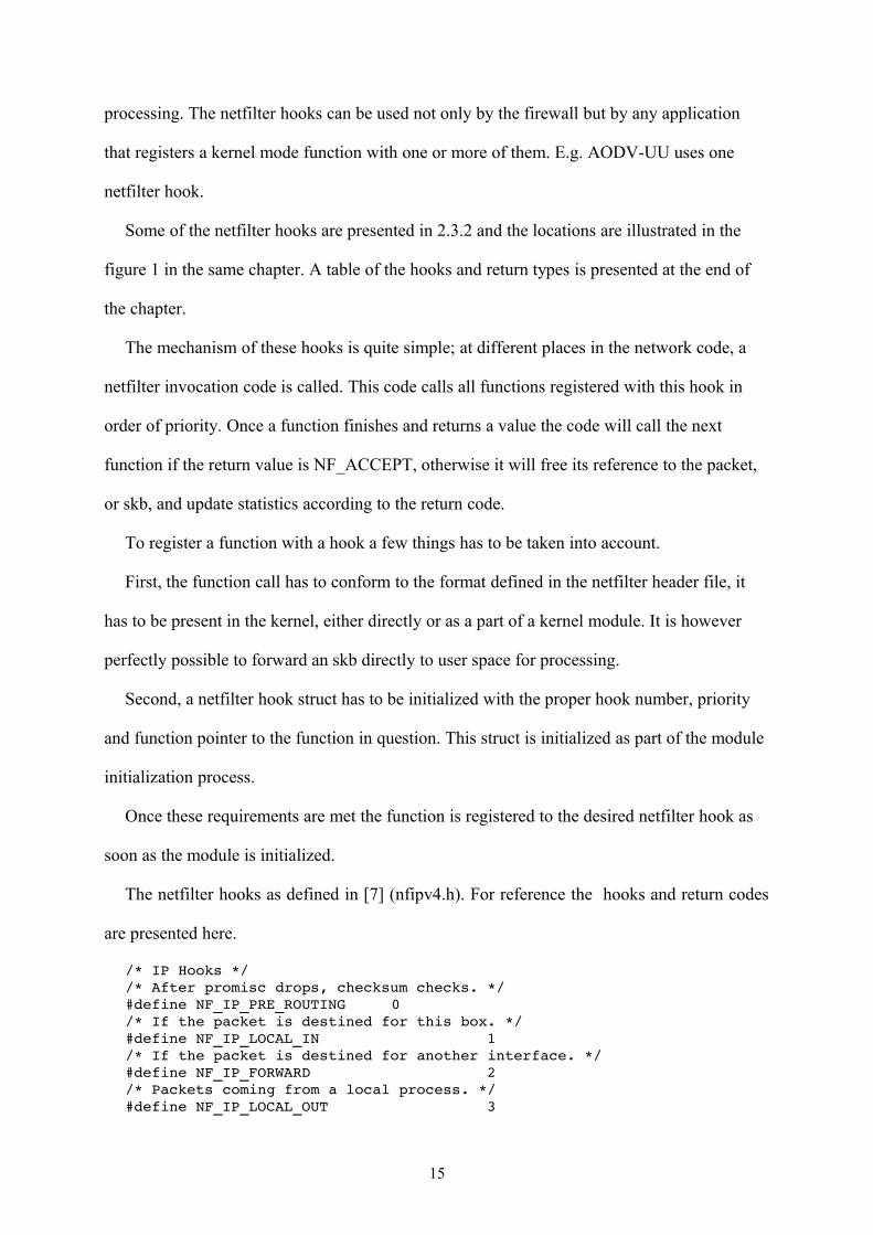
The netfilter hooks as defined in [7] (nfipv4.h). For reference the hooks and return codes
are presented here.
/* IP Hooks *//* After promisc drops, checksum checks. */#define NF_IP_PRE_ROUTING 0/* If the packet is destined for this box. */#define NF_IP_LOCAL_IN 1/* If the packet is destined for another interface. */#define NF_IP_FORWARD 2/* Packets coming from a local process. */#define NF_IP_LOCAL_OUT 3
15
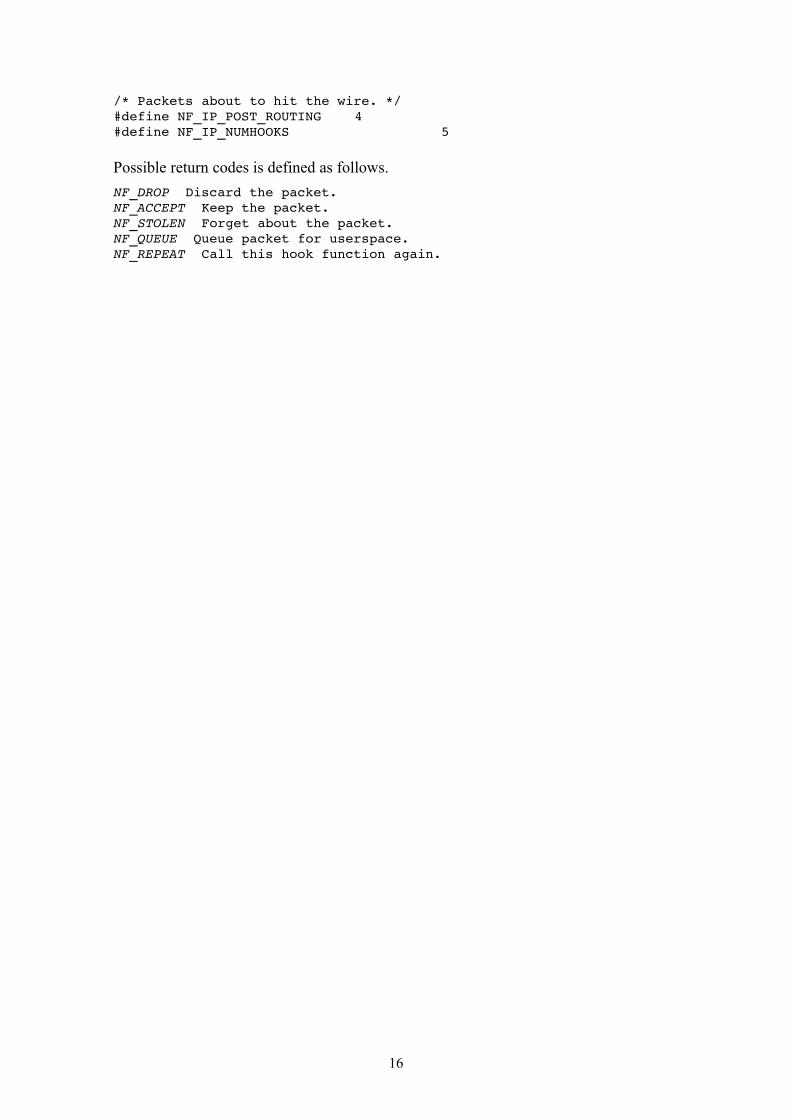
/* Packets about to hit the wire. */#define NF_IP_POST_ROUTING 4#define NF_IP_NUMHOOKS 5
Possible return codes is defined as follows.
NF_DROP Discard the packet. NF_ACCEPT Keep the packet. NF_STOLEN Forget about the packet. NF_QUEUE Queue packet for userspace. NF_REPEAT Call this hook function again.
16
2.4 Ad hoc On-Demand Distance Vector (AODV)
The AODV [9] routing protocol is a routing protocol designed for ad hoc mobile networks.
The protocol builds paths between nodes upon request from a source node, and maintains
these paths as long as they are needed. A node is here considered to be a AODV capable
computer or router.
AODV builds routes using a cycle of route requests and route reply. When a source host
wants to find a path to a unknown destination it broadcasts a route request (RREQ). The
RREQ contains the addresses of the source and the destination, a broadcast identifier and the
most recent sequence number for the destination of which the source is aware. Nodes
receiving this broadcast message update their information on their source node and set up
backwards pointers to the source node in the route tables. The node may then send a route
reply (RREP) if it is the destination or if it has a route to the destination with a sequence
number equal to or higher than that in the RREQ. If not, the node will rebroadcast the RREQ.
Since the nodes store the broadcast identifier and the source and destination address, the
nodes will be aware if they receive a RREQ it has already seen, and discard it to avoid loops
of route requests.
As the RREP is sent back to the source, the nodes set up forward pointers to the
destination. When the source node receives a route reply it can begin to send data packets
across the network. If the source receives another RREP with information of a better route,
the source may switch to the newer route.
17
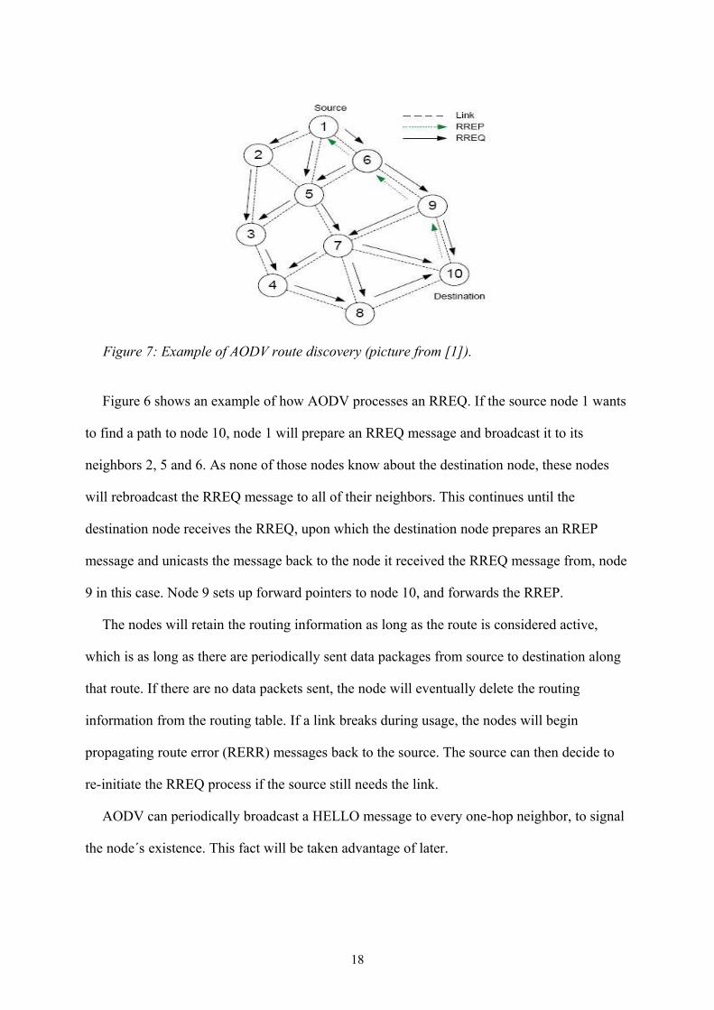
Figure 6 shows an example of how AODV processes an RREQ. If the source node 1 wants
to find a path to node 10, node 1 will prepare an RREQ message and broadcast it to its
neighbors 2, 5 and 6. As none of those nodes know about the destination node, these nodes
will rebroadcast the RREQ message to all of their neighbors. This continues until the
destination node receives the RREQ, upon which the destination node prepares an RREP
message and unicasts the message back to the node it received the RREQ message from, node
9 in this case. Node 9 sets up forward pointers to node 10, and forwards the RREP.
The nodes will retain the routing information as long as the route is considered active,
which is as long as there are periodically sent data packages from source to destination along
that route. If there are no data packets sent, the node will eventually delete the routing
information from the routing table. If a link breaks during usage, the nodes will begin
propagating route error (RERR) messages back to the source. The source can then decide to
re-initiate the RREQ process if the source still needs the link.
AODV can periodically broadcast a HELLO message to every one-hop neighbor, to signal
the node´s existence. This fact will be taken advantage of later.
18
Figure 7: Example of AODV route discovery (picture from [1]).
2.4.1 AODV-UU
AODV in itself is proposal by the IETF(RFC 3561) and not an implementation. There are
two RFC compliant implementations; KERNEL-AODV NIST and AODV-UU.
During this project the later is chosen since [1] suggested an extension of AODV-UU, and
since AODV-UU works on Linux kernel 2.4 as well as 2.6, while KERNEL-AODV requires
kernel version 2.4.
AODV-UU was created by Erik Nordström[10] at Uppsala University, hence the UU
suffix. It is implemented as a user-space daemon with a kernel component. The most current
release at the time of writing is 0.9.5.
2.5 OpenWrt on Linksys
One of the goals of this project is to get a packet aggregation working on a cheap
standardized commercial networking platform. The rationale behind this is that packet
aggregation is first and foremost a scheme to enhance over all performance by enhancing
performance over each link [1].
2.5.1 The Linksys WRT54GL version 1.1
This is the router of choice in this project because it is easily available and is sold as a
router for enthusiasts who want to install their own firmware on it [18].
Due to its relative fame in ”enthusiast” circles there are many different firmwares to
choose from for this particular router, many of which originate from the OpenWrt project.
OpenWrt is basically a Linux system and a cross compiler tool chain which makes it
possible to run the Linux system on a variety of machines including the Linksys WRT 54GL.
OpenWrt will be described in detail later in this chapter.
The Linksys WRT 54GL in a standard wireless router with a 10/100Mbit Ethernet wan
port and a 4 port 10/100 M bit switch and a 802.11g wireless interface with two antennae. It
19
has a Broadcom 5352 chip set with integrated wireless interface. Broadcom 5352 has a MIPS
32bit cpu which in this case is clocked at 200 MHz. It has an 8Mbyte flash memory and
16Mbyte ram. In its original configuration the settings is saved in an NVRAM.
2.5.2 OpenWrt
OpenWrt started off as a project to get a free and fully customizable firmware on the
Linksys WRT 54G routers which Linksys had used a Linux-based firmware on and therefore
published the source code for.
The first generation of OpenWrt firmware was codenamed White Russian (after the drink)
and was specialized for the Linksys router and similar Broadcom based routers. It used Linux
2.4 kernel and saved its configuration settings in the NVRAM.
The second and current generation of OpenWrt is codenamed Kamikaze (also after a
drink). This version is interesting due to the fact that it uses configuration files to save the
settings like a normal Linux system. It is targeted towards a much wider range of appliances,
from ADSL modems to Playstation3. It uses either the 2.6 or the 2.4 kernel depending on
what works best for that particular device.
2.6 Summary.
In this chapter, information about components used in the implementation has been
presented. Information about aggregation as a concept was presented in chapter 2.2, and in
chapter 2.3 Linux networking including the socketbuffer or skb, Queueing diciplines or
Qdisc, the control tool tc or traffic control and Netfilter was presented with figure 1 as a
simple illustration. In 2.4 AODV routing and the AODV-UU implementation was presented.
And in 2.5 OpenWrt and the Linksys WRT54GL was presented.
20
3 Implementation
3.1 Introduction
This chapter gives a detailed description of some possible solutions and one approach to
implementing packet aggregation in Linux. Section 3.2 describes possible solutions for packet
aggregation and includes the reasoning for why the specific solution was chosen. The chosen
implementation consists of an aggregation module, presented in section 3.3.3, and a
deaggregation module described in section 3.3.4. The aggregation module can only deal with
skb packets that are intended to go to a destination that supports aggregation and since there
are many destinations which potentially do not support aggregation, a parent qdisc to the
aggregation module has been designed, which is described in section 3.3.2. Furthermore, a
new packet format, the IP meta packet, is defined in section 3.3.1. Section 3.4 is a proposal
for an optional extension of the AODV-UU for distributed measuring of link quality, which
could be used together with dynamic marking. Dynamic marking is explained in section
3.3.3.1.
3.2 Different approaches to packet aggregation
We have considered three different approaches to packet aggregation in Linux. They range
between a user space application and a complete integration in the Linux networking stack.
3.2.1 Implementation as a user space application
The user space application approach has the primary benefits of easy coding and well
defined boundaries, it would be fairly easy to port to other versions of the Linux kernel. Since
coding for user space gives us access to all common libraries, little extra effort would be
needed to find information on the specific functionalities we require. Also the environment is
21
familiar. Both aggregation and deaggregation can be done in the same application. This
approach needs a small kernel module for catching packets for aggregation and possibly a
virtual device for reinserting deaggregated packets into the networking stack.
The primary drawback of a user space application is performance and missed aggregation
opportunities. Performance is of course important to a system with limited resources such as
the Linksys router and the fact that routing of VoIP packets is an extremely time critical
operation due to latency and jitter constraints. This approach raised some questions in regards
to the cost of transporting skb to and from user space and the efficiency of the code in user
space.
The issue with missed aggregation opportunities can be explained by the use of two
queues. The first queue in the aggregation application accumulates packets for aggregation
but it has to send the packets if the forced delay time expires, even if it has not reached the
size threshold. When it has sent the aggregated packet it is enqueued in the network queue in
the device where it could be held up, for example due to the network media not being free. If
another packet is received by the aggregation application before the previously aggregated
packet is dequeued from the network queue, there is no way to add this new packet to the one
already in the network queue. This is a missed aggregation opportunity.
3.2.2 Implementation as a kernel module
The second approach is very similar to the first with the exception that the application is
implemented as a kernel module. This approach shares some of the previous approaches´
benefits in that it is a well defined piece of code with a clear interface to the rest of the kernel
making it very portable (across different kernel versions). Kernel space programming does
however require that one can implement the desired functionality with the types and
operations already in the kernel. Unfortunately documentation of the Linux kernel code is
sparse and often outdated, since it is constantly developed, including new functionality
deprecating old and just generally changing available methods and structures to fit the current
22
development. This allows for good development but make kernel API's constantly changing.
The best way to come to understand the kernel is to simply read the source code and try to
figure out what can be used and how.
The benefit of implementing the application as a module in kernel space is performance,
the cost of transporting data between kernel space and user space is eliminated. This second
approach still has the problem of double queues. So the problem with missed opportunities
still exists.
3.2.3 Implementation directly in networking stack
The third approach is to put our aggregation directly in the networking stack by creating
a queue which aggregates packets and can be attached to any network interface. This
approach suffers no special performance penalty since it is in kernel space and it uses no extra
queue. The problem of missed opportunities is partly solved. The only extra queue present is
the cache on the network device but this is very small, usually only enough for one packet.
To solve this the implementation has to be placed in the driver, which would make it driver
specific and not an appropriate solution for a general implementation.
The discussion so far has been concentrated on aggregation and since it is possible to
create a custom queue, or Qdisc, and attach it to any network device on the egress queue it is
a good thing to do but only one “queue” or Qdisc can be attached on the ingress side namely
the ingress Qdisc which is not a queue at all and only implements a kind of traffic policing.
So the deaggregation has to be implemented in a manner similar to the second approach,
implementation as a kernel module with netfilter, but since we do not have the problem of
double queues here, this does not present a problem.
3.2.4 Conclusions
Of these three approaches, the third one is preferable from a performance point of view. As
has been shown, both implementation as a user space application and as a kernel module will
23
result in code which is well defined and easily ported. Performance is however a major
concern in the implementation of a algorithm specifically designed to increase performance
of, in this case, VoIP traffic. Another concern is the performance in smaller network routers.
This issue with performance is the reason why approach three, implementation directly in the
network stack, was chosen.
3.3 Implementation
3.3.1 Packet Layout
The IP Meta header
The IP meta header is the IP header of the aggregated packet. The IP meta header is an IP
version 4 header. The header length is always 20 bytes since no options are allowed and the
protocol field is set to a value that our deaggregation module will recognize – currently 253.
This value was chosen as it is reserved for experimentation[11].
Meta packet structure
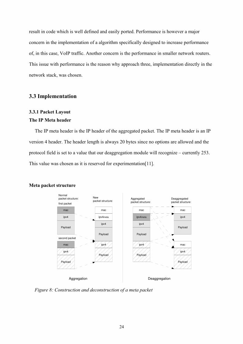
24
Figure 8: Construction and deconstruction of a meta packet
mac
ipv4
Payload
mac
ipv4
Payload
Normal packet structure:
first packet
second packet
mac
ipv4
Payload
ipv4
Payload
New packet structure:
ipv4meta
mac
ipv4
Payload
mac
ipv4
Payload
Deaggregated packet structure:
mac
ipv4
Payload
ipv4
Payload
Aggregated packet structure:
ipv4meta
Aggregation Deaggregation
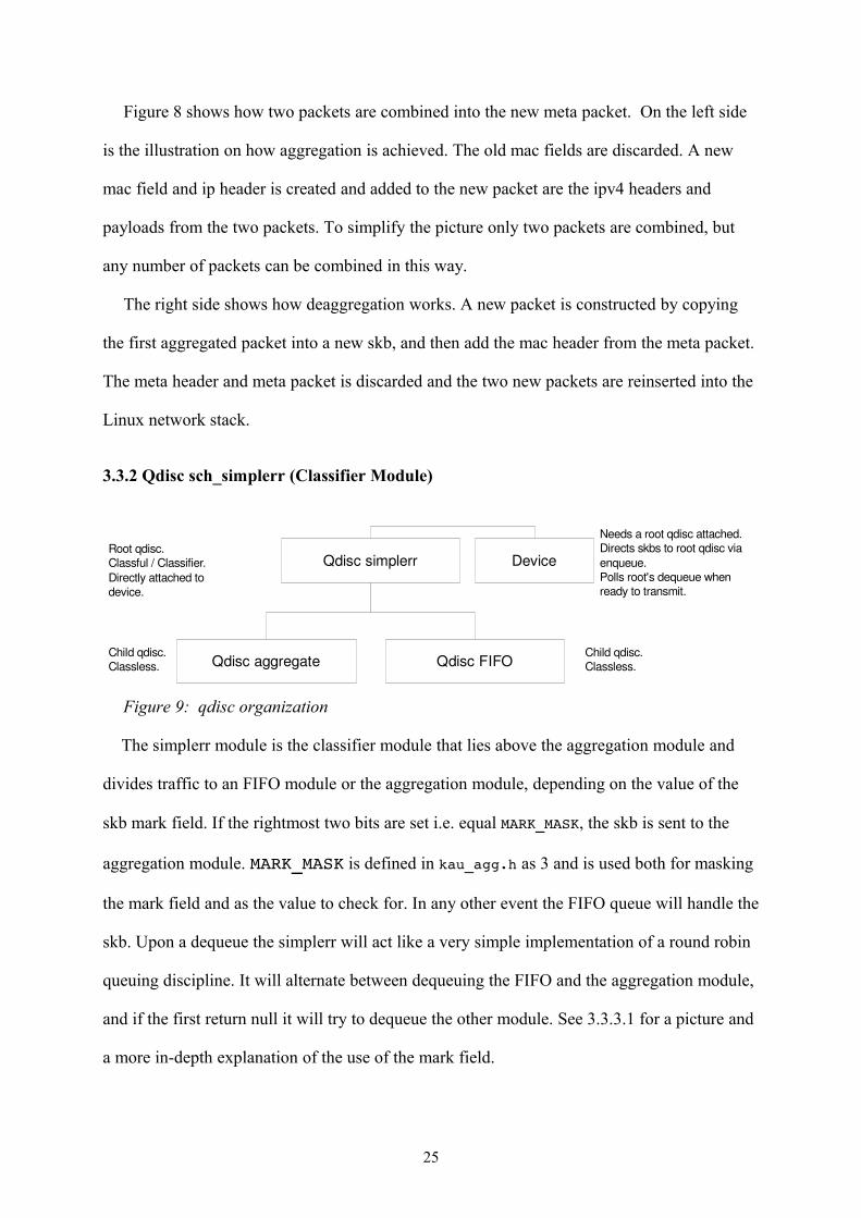
Figure 8 shows how two packets are combined into the new meta packet. On the left side
is the illustration on how aggregation is achieved. The old mac fields are discarded. A new
mac field and ip header is created and added to the new packet are the ipv4 headers and
payloads from the two packets. To simplify the picture only two packets are combined, but
any number of packets can be combined in this way.
The right side shows how deaggregation works. A new packet is constructed by copying
the first aggregated packet into a new skb, and then add the mac header from the meta packet.
The meta header and meta packet is discarded and the two new packets are reinserted into the
Linux network stack.
3.3.2 Qdisc sch_simplerr (Classifier Module)
The simplerr module is the classifier module that lies above the aggregation module and
divides traffic to an FIFO module or the aggregation module, depending on the value of the
skb mark field. If the rightmost two bits are set i.e. equal MARK_MASK, the skb is sent to the
aggregation module. MARK_MASK is defined in kau_agg.h as 3 and is used both for masking
the mark field and as the value to check for. In any other event the FIFO queue will handle the
skb. Upon a dequeue the simplerr will act like a very simple implementation of a round robin
queuing discipline. It will alternate between dequeuing the FIFO and the aggregation module,
and if the first return null it will try to dequeue the other module. See 3.3.3.1 for a picture and
a more in-depth explanation of the use of the mark field.
25
Figure 9: qdisc organization
Qdisc simplerr
Qdisc aggregate Qdisc FIFO
DeviceRoot qdisc.Classful / Classifier.Directly attached to device.
Child qdisc.Classless.
Child qdisc.Classless.
Needs a root qdisc attached.Directs skbs to root qdisc via enqueue.Polls root's dequeue when ready to transmit.
There are two fields in the qdisc struct that are used by the attached device to determine
whether the qdisc is holding any skbs. It is important to update these fields properly since the
device will be relying on them when determining if the dequeue of the root qdisc should be
called. The fields are inside the following two structs, both structs are instantiated in the qdisc
struct.
struct sk_buff_head q;
struct gnet_stats_queue qstats;
The skb_buff_head struct contains the field qlen which needs to be the exact number of
skbs that the simplerr module is handling. The gnet_stats_queue struct contains the field
backlog which needs to be the combined size – in bytes – of all those skbs. When the simplerr
receives an skb to enqueue, the qlen and backlog is simply updated with the new information.
At a dequeue from the FIFO module, the values of qlen and backlog are simply reduced by
one and the size of the skb respectively. When the aggregation module is dequeued the
simplerr module must first save the current length of the skbs inside the aggregation module,
as well as the number of skbs enqueued before calling the aggregation module's dequeue
function. After the dequeue, simplerr must compare the old information with the current size
and the number of skbs to correctly set qlen and backlog.
The above approach was chosen as the default approach of retrieving the information from
the skb returned by the aggregation module will not work, since there is no indication of how
many skbs have been bundled together. When the aggregation module receives an skb, the
skb will contain a complete packet with a mac header, IPv4 header and a payload. When
simplerr calls the aggregation module's dequeue method, the aggregation module will try to
bundle together several skbs' ipv4 header and payload, discarding all the mac headers. The
aggregation module will then add a new IPv4 header - the meta header, see chapter 3.3.1 –
and one new mac header on top. As the mac header is included in every skb given to the
aggregation module but only one is included in the returned skb, the length of any number of
26
mac headers could potentially be lost. This creates a dependency between the simplerr module
and the aggregation module.
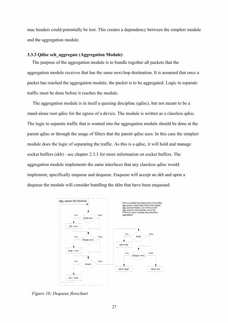
3.3.3 Qdisc sch_aggregate (Aggregation Module)
The purpose of the aggregation module is to bundle together all packets that the
aggregation module receives that has the same next-hop destination. It is assumed that once a
packet has reached the aggregation module, the packet is to be aggregated. Logic to separate
traffic must be done before it reaches the module.
The aggregation module is in itself a queuing discipline (qdisc), but not meant to be a
stand-alone root qdisc for the egress of a device. The module is written as a classless qdisc.
The logic to separate traffic that is wanted into the aggregation module should be done at the
parent qdisc or through the usage of filters that the parent qdisc uses. In this case the simplerr
module does the logic of separating the traffic. As this is a qdisc, it will hold and manage
socket buffers (skb) - see chapter 2.3.3 for more information on socket buffers. The
aggregation module implements the same interfaces that any classless qdisc would
implement, specifically enqueue and dequeue. Enqueue will accept an skb and upon a
dequeue the module will consider bundling the skbs that have been enqueued.
27
Figure 10: Dequeue flowchart
if(large<curr)
if(old<curr)
old = curr;
large = curr;
if(next)
curr = next;
if(old)
if(large>=min)
return old;
return large; return null;
True
True
True
True
True
False
False
False
False
False
agg_queue list traversalold is a variable that keeps track of the oldest agg_queue. large keeps track of the largest agg_queue(in bytes). curr is the current agg_queue in the traversal. min is the minimum value (in bytes) that should be aggregated.

Figure 10 illustrates the algorithm used by the aggregation module to decide what it should
dequeue. One agg_queue holds every skb going to the same next-hop destination, as well as
information pertaining to those skbs. The module will hold an skb as long as the skb is not
considered too old, or until enough skbs going to the same next-hop have been accumulated
and the size threshold has been reached. For more information on agg_queues and how to
configure the time before an skb is considered “too old” and size threshold , see next section.
There are several scenarios that could happen upon a dequeue;
1. If one skb is enqueued into the module and not enough other skbs going to the
same next-hop are enqueued to reach the size threshold, the skb will be considered too
old after a time, which can be configured via tc, and will be sent out upon a dequeue.
2. If several skbs for the same next-hop have been accumulated, the size threshold
will be reached. Upon a dequeue a new skb large enough to hold all the skbs and a
new IP header will be created. The information in the old skbs will be copied into the
new skb, and a the IP meta header will be created and inserted. The old skbs will be
destroyed, and the new skb is given to the parent simplerr. The parent will then give
the new skb to the device the parent is attached to, and the device will begin
transmission.
3. If the module determines that the skbs enqueued are not old enough and the size
threshold is not reached, the module will return null on a dequeue. This does not mean
that the module is empty - just that nothing met the criteria and was allowed to be sent.
If there are more skbs in queue than what is allowed to be sent across the link, the module
will only bundle together skbs up to the maximum allowed size. Next-hop queues (explained
in next section) keeps track of the oldest skb in the queue. The oldest next-hop queue is
always considered first, even when there are larger next-hop queues available.
28
Aggregation Module – Implementation
In order to bundle together skbs, at least two skbs have to be enqueued. A list capable of
keeping skbs is needed, and fortunately provided by the Linux kernel. The interface for the
list capable of maintaining skbs can be found in the file /net/linux/sk_buff.h.
The enqueued skbs can have different destinations but bundling skbs can only be done on
skbs with the same next-hop destination. Keeping one list with all skbs would mean that the
dequeue function would have to traverse the entire skb list every time to find the total size of
skbs for every next-hop destination, as well as finding if there is an skb that needs to be sent
due to timeout. To simplify this process a new struct and an interface was created. The point
of this new struct is to create an skb queue for every next-hop destination - instead of just one
– and to save certain information regarding that particular skb queue in a easily accessible
field. The new struct is defined as:
struct agg_queue{
__be32 dest; __u32 currSize;__u32 maxSize;psched_time_t timestamp;struct agg_queue *next;struct sk_buff_head skb_head;
};
Where:
● dest is the next-hop destination for all the skbs.
● currSize is the combined size of all skbs.
● maxSize is the maximum allowed size in bytes that the link between the current
node and the next node can handle.
● timestamp is the timestamp of the oldest packet in the skb list, which is the first
skb that arrived in the enqueue for this particular next-hop destination.
● next is a pointer to the next skb list, with another next-hop destination. This is
null if there are no more destinations.
29
● skb_head is the beginning of the skb list, and this list only contains skbs going to
the same next-hop destination. The skb list is used as an FIFO list.
All qdiscs implement a private struct where private variables are entered. A pointer to the first
next-hop destination is put inside. Definition follows.
struct aggregate_sched_data {
struct qdisc_ watchdog watchdog; unsigned int agg_min_size;
unsigned int agg_max_size; unsigned int agg_max_timeout; struct agg_queue *agg_queue_hdr;
};
● With the use of the head – agg_queue_hdr - node and the next field in the struct, a
list is implemented – with one entry for every next-hop destination.
● The agg_min_size field is the minimum size in bytes that the individual next-hop
destination queues need to reach before they are considered for aggregation, assuming
they do not get sent because they are considered to be too old. This field can be set by
the -min flag with tc. If not set, this field will default to AGG_MIN_LENGTH defined in
kau_agg.h.
● The agg_max_size field can be set by using the -max flag with tc, and is heavily
entwined with maxSize in the agg_queue declaration. See 3.3.3.1 for more
information. If not set, this field will default to AGG_MAX_LENGTH defined in
kau_agg.h.
● The agg_max_timeout field is used to determine the maximum amount of time in
microseconds that the module can hold a packet. If the packet is held longer than
agg_max_timeout, it is considered to be old, and must be sent as soon as possible.
This field can be set by the -timeout flag using tc. If not set, this field will default to
TIME_PAD defined in kau_agg.h.
● Watchdog is a built-in struct with a interface that allows the aggregation module to
ask the device the qdisc is attached to, to call the dequeue function at a specific time.
30
This is used to schedule another dequeue when the aggregation module will return
null, to ensure that the device polls the aggregation module regularly.
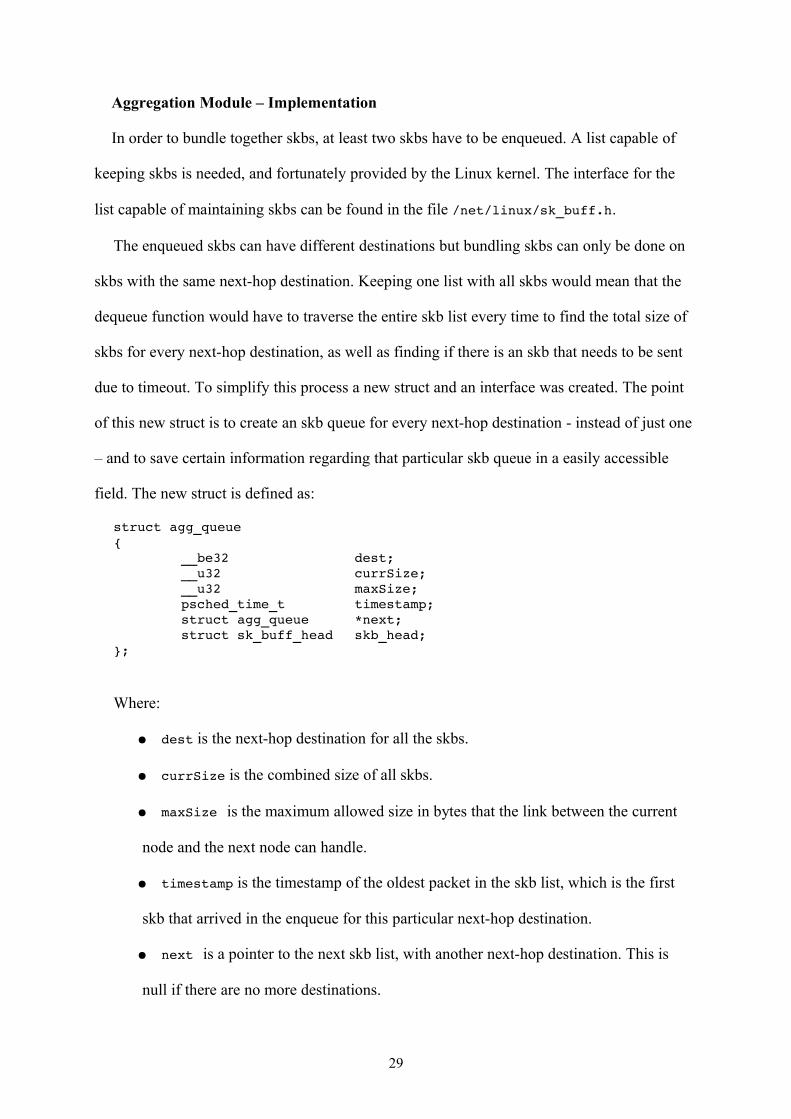
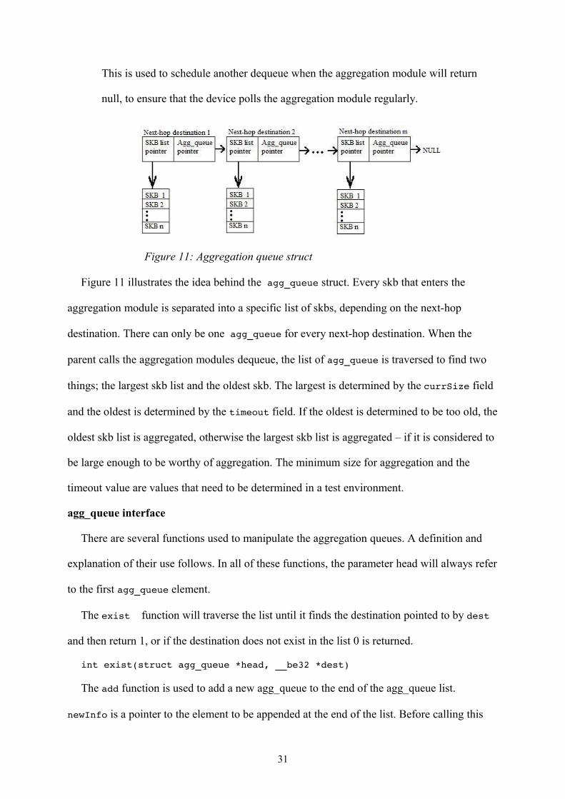
Figure 11 illustrates the idea behind the agg_queue struct. Every skb that enters the
aggregation module is separated into a specific list of skbs, depending on the next-hop
destination. There can only be one agg_queue for every next-hop destination. When the
parent calls the aggregation modules dequeue, the list of agg_queue is traversed to find two
things; the largest skb list and the oldest skb. The largest is determined by the currSize field
and the oldest is determined by the timeout field. If the oldest is determined to be too old, the
oldest skb list is aggregated, otherwise the largest skb list is aggregated – if it is considered to
be large enough to be worthy of aggregation. The minimum size for aggregation and the
timeout value are values that need to be determined in a test environment.
agg_queue interface
There are several functions used to manipulate the aggregation queues. A definition and
explanation of their use follows. In all of these functions, the parameter head will always refer
to the first agg_queue element.
The exist function will traverse the list until it finds the destination pointed to by dest
and then return 1, or if the destination does not exist in the list 0 is returned.
int exist(struct agg_queue *head, __be32 *dest)
The add function is used to add a new agg_queue to the end of the agg_queue list.
newInfo is a pointer to the element to be appended at the end of the list. Before calling this
31
Figure 11: Aggregation queue struct
function, a check must be made to make sure that the destination field in newInfo is unique.
That is, there can be no other agg_queues in the list that is going to the same next-hop
destination. If there already is an agg_queue with the destination in the list, addSkb should be
used.
void add(struct agg_queue* head,struct agg_queue* newInfo)
The addSkb function finds the agg_queue with the same destination as dest, and adds the
incoming skb to the end of that destinations skb list.
void addSkb(struct agg_queue* head, struct sk_buff *skb, __be32 *dest)
The remove function completely removes the agg_queue where the destination equals
dest. If there are skbs in the agg_queue, these will be removed.
int remove(struct agg_queue **head, __be32 *dest)
The purpose of the getDequeue function is to find the oldest skb and the largest skb list in
the agg_queue list. If it finds an skb that is considered to be too old, the agg_queue that the
skb is in is returned. If nothing old is found, the largest skb list is returned if it is considered to
be large enough. NULL is returned if nothing matches the criteria. The field
min_aggregation is set to agg_min_size. If do_mark_update is 1, dynamic marking is
used. The watchdog is used to schedule another dequeue from the device if getDequeue is
about to return null.
struct agg_queue* getDequeue(struct agg_queue* head, unsigned int min_aggregation, unsigned int do_mark_update, struct qdisc_watchdog *watchdog)
3.3.3.1 About maxSize, agg_max_size, -max and dynamic marking
The maxSize can be used in several ways, and can be set by tc using the -max flag if static
marking is intended. If max is not set, agg_max_size will default to AGG_MAX_LENGTH,
currently set to 1500 and defined in kau_agg.h, which in turn will set maxSize for every new
next-hop destination queue to 1500. If agg_max_size is set to 0, the module will allow for
dynamic marking, any other value will set maxSize to the same value as agg_max_size.
32
Dynamic marking allows the aggregation module to change the value of maxSize
whenever a new skb is received. The module will do this by first shifting the mark field two
bits to the right and then look at the 16 least significant bits of the mark field, and save the
value in the maxSize field. This implies that all skbs that enter the aggregation module when
in dynamic mode must have the mark field set. The agg_max_size field can be statically set
to anything between 100 and 2048 by using the max flag with tc, anything outside those
boundaries will make agg_max_size default to AGG_MAX_LENGTH. The dynamic marking
method can be used to only allow the module to send packets as large as the receiving node
can handle, but a valid method of calculating the maximum size for such a packet is beyond
the scope of this essay.
Figure 12 illustrates the use of the mark field for traffic separation in the classifier module
- see chapter 3.3.2 – as well as the bits used in dynamic marking.
3.3.4 deaggregate (Deaggregation Module)
The main function of the deaggregation module is to identify aggregated packets and to
restore the original packets from the meta packet and then reinsert them into the network
stack. This should be done in a way that does not interfere with the handling of ordinary
traffic and the original packets should be reinserted at a place where they will not bypass
ordinary firewall processing.
33
Figure 12: The mark field
11
two bit shift
The bits used in dynamic marking
The 32 bit skb>mark field
Bits used by classifier for traffic separation
One appealing idea is to implement a queue similar to the aggregation queue since it
would reside as an attachment to the device and be handled in much the same way as
aggregation with tc. But after some investigation into the ingress queue, which is part of the
Linux kernel and can be handled with tc, the arguments against such an approach, presented
below, weighs against it and an implementation using netfilter seems a better choice.
The main reason not to redesign the ingress queue is that it is in fact not a queue at all but a
filter. The documentation [Linux source] describes a policing filter. It is of course logical
since the reason to have a queue such as an egress queue (to wait for the medium to be free)
does not exist on the inbound side, the reception of a packet is handled by the device driver
and once a packet is delivered to memory it is more a matter of process scheduling at the
processor. A queue implementation would mean to add an artificial delay and a dequeue call
which is not necessary and would interfere with normal traffic.
To implement a module based on netfilter is on the other hand quite easy and follows the
general principles of the Linux kernel better. The biggest problem with this approach is to
reinsert the original packets into the correct place in the network stack.
The principle of the final implementation is to register a function with the first incoming
netfilter hook, this means that as soon as a packet passes the point in the network stack where
the netfilter hook is, then all functions registered to this hook are called in order based on
priority. The deaggregation function is registered with priority PRI_FIRST which ensures that
all packets pass by this function first, thus eliminating the risk that aggregation packets could
be discarded by other firewall rules or other functions registered to this hook.
To minimize the risks with the high priority by using a quick inspection of the packet and
to release all non meta packets as soon as possible also minimizing the processing overhead
on ordinary traffic.
Once a meta packet is found the deaggregation function can extract the original packets
one by one and insert them into the network stack. This is done by constructing a new skb,
34
copying the mac header from the original meta packet and then calling netif_rx which is a
function that device drivers call to insert a newly received packet into kernel memory. This
approach ensures that we do not miss any aggregated packets and the inserted packets will be
subjected to ordinary firewall operations.
Short introduction to the deaggregation code
For an easier understanding of the initialization function, this will be described first as it
explains some of the design choices in the main deaggregation function.
struct nf_hook_ops deaggregate
static int __init deagg_module_init(void)
The initialization function, deagg_module_init, has the responsibility to initialise the
nf_hook_ops struct, which is defined in netfilter.h and instantiated as deaggregate, with a
function pointer to the deaggregation function, protocol family, netfilter priority, netfilter
hook and module owner, and then to register deaggregate with netfilter. It also does a printout
to the kernel log just to log that it is loaded.
The initialisation and registration of the nf hook options tells the netfilter module to pass
all packets to the designated function, in this case deaggregation(), at the hook specified with
hooknum (NF_IP_PRE_ROUTING), with the protocol in pf (PF_INET i.e. IP) and in order of
the priority set by priority (NF_IP_PRI_FIRST). This of course sets a format for the function
to implement, it has to return a valid netfilter return value and it has to accept the correct
parameters.
deaggregation(hooknum, **skb, *in,*out,int (*okfn)(struct sk_buff *) )
Deaggregation is the actual function which is called by netfilter and contains nearly all the
logic in the deaggregation module.
35
3.3.5 Installation and configuration
Kernel configuration
To use the aggregation and the deaggregation modules they have to be compiled together
with the kernel, essentially as a part of the kernel. This requires that the source files are placed
in the correct part of the kernel source directory structure as described below. The following
adjustments to the kernel make files is also necessary to let make know about the new
modules.
The directory structure referred to is originating in the Linux source directory. The files to
place at the right place is kau_agg.h in include/net/, deaggregate.c in
net/sched/ ,sch_simplerr.c in net/sched/ and sch_aggregate.c in net/sched/
Makefile and Kconfig in net/sched/ contains the information about code in this
directory and has to be changed to include information about the new modules. Kconfig is
read by configuration utilities such as menuconfig and includes information about the
different modules as text and defines the configuration switches to include in the .config file,
should a module be chosen for inclusion as a module or directly linked into the kernel. The
Makefile has the target definitions in the directory.
A passage similar to
config NET_SCH_AGGREGATE tristate "KAU_AGG" help <informative text>
has to be added to Kconfig for every module that should be able to be included in the
kernel.
config NET_SCH_AGGREGATE is the definition which is used by the configuration utility
to define the target CONFIG_NET_SCH_AGGREGATE in the Makefile.
tristate “KAU_AGG” means that the menu entry KAU_AGG in menuconfig can be
chosen as not included, included as a module or linked directly into the kernel.
36
The text below help is purely a help text intended to inform the one who is
configuring the kernel about the particular module.
In the Makefile a line similar to
obj$(CONFIG_NET_SCH_AGGREGATE) += sch_aggregate.o
has to be added for every module that is to be compiled.
Once the changes in Kconfig Makefile and the files are copied to the right place, the new
kernel including the new modules can be built by configuring the kernel with make
menuconfig or any configuration utility of choice and the running make, or make modules if
only the modules are of interest and then installing them with make modules_install.
tc configuration
tc, the tool used to mount and control qdiscs, needs to have the file q_simplerr.c and the
following changes to be aware of the new qdisc. The add-on needs to be compiled together
with the rest of iproute2, which is “a collection of utilities for controlling TCP / IP networking
and traffic control in Linux”[12]. Since simplerr is used as a parent to the aggregation
module, the add-on only includes simplerr. The source code for the add-on is in q_simplerr.c,
and this file should be placed inside the /iproute2-(version)/tc/ folder, then compiled together
with the rest of iproute2 by doing a 'make' and 'make install' in the iproute2 root directory.
The source code for this add-on is supplied as appendix 5. The Makefile inside the tc
directory might be need these lines added to compile q_simplerr.c. correctly;
TCMODULES += q_simplerr.oq_simplerr.so: q_simplerr.c
$(CC) $(CFLAGS) shared fpic o q_simplerr.so q_simplerr.cthe 'all:' statement needs to be changed to:
all: libtc.a tc $(TCSO) q_simplerr.so
If everything compiled correctly, the file q_simplerr.so should appear in directory
/usr/lib/tc/. If it is missing, it will be inside the /iproute2-(version)/tc/ folder, and it needs to be
moved to the correct location manually.
37
Loading and usage
To be able to mount the qdiscs to the egress of a device the modules will first need to be
loaded. Loading the modules can be done in two ways; using modprobe command or the
insmod command. modprobe requires the modules to be placed inside /lib/modules/<kernel
version>/[13], while insmod[14] simply accepts any location specified. To load with
modprobe, write; 'modprobe <module_name>'. In this case, writing
modprobe sch_simplerrwill load the simplerr module. This will also cause the aggregation module to load. With
the use of insmod however, you must first load the aggregation module and then the simplerr
module. This is because modprobe reads and loads the dependencies, while insmod does not.
To load the modules with insmod write 'insmod /<location>/<module_name>' or in this case
(In that order.)
insmod /location/sch_aggregate.ko insmod /location/sch_simplerr.ko
Next is to mount the simplerr module as the root qdisc for the egress of a device. This is
done using the following command:
tc qdisc add dev DEVICE_ID root simplerr.
This will make the simplerr module load, and all because no parameters are specified all
the default values of the aggregation module are used. Write ifconfig to get a listing of every
available device and their corresponding ID. Parameters can also be specified by using the
following syntax:
tc qdisc add dev DEVICE_ID root simplerr timeout X min Y max Z
timeout will set the agg_max_timeout field, min will set the agg_min_size field and max
will control the agg_max_field. For more information see section 3.3.3.
To load the deaggregation module is equally simple;
modprobe deaggregate
if the module is correctly placed, or the below if the module is placed somewhere else.
insmod /location/deaggregate.ko
38
Now the aggregation module is loaded and ready to aggregate, and the deaggregate module
is loaded and waiting. To unload the the aggregation module and simplerr, simplerr must first
be dismounted as the root egress device with tc.
tc qdisc del dev eth1 root
After this the modules can all be unloaded with rmmod, by typing 'rmmod
<module_name>'. For example;
rmmod sch_simplerr
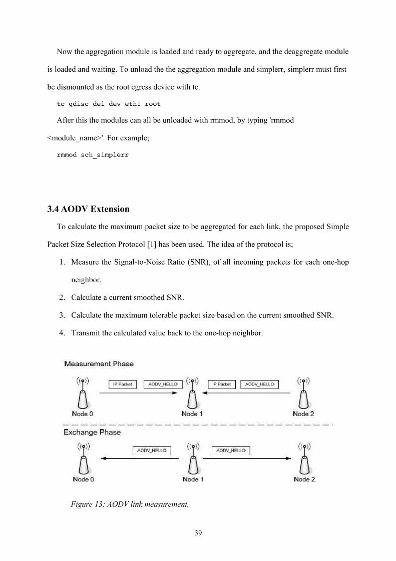
3.4 AODV Extension
To calculate the maximum packet size to be aggregated for each link, the proposed Simple
Packet Size Selection Protocol [1] has been used. The idea of the protocol is;
1. Measure the Signal-to-Noise Ratio (SNR), of all incoming packets for each one-hop
neighbor.
2. Calculate a current smoothed SNR.
3. Calculate the maximum tolerable packet size based on the current smoothed SNR.
4. Transmit the calculated value back to the one-hop neighbor.
39
Figure 13: AODV link measurement.
Figure 13 illustrates this behavior. Node 1 receives packets from Node 0 and Node 2. Node
1 will calculate the maximum tolerable packet size for each of the two links; Node 0 -> Node
1 and Node 2 -> Node 1; and then add the information to the AODV HELLO message that is
periodically broadcasted to all one-hop neighbors. Node 0 and Node 2 will receive the
HELLO, divide the message and find the entry that is specified to belong to them and then
retrieve the maximum packet size allowed on this link. The extended HELLO message from
Node 1 looks like this;
[HELLO][AddrNode0][PSnode0][AddrNode2][PSnode2]
Where:
● AddrNode0 is the IP address of Node 0.
● PSnode0 is the maximum tolerable packet size when Node 0 wants to send a packet to
Node 1.
● AddrNode2 is the IP address of Node 2.
● PSnode2 is the maximum tolerable packet size when Node 2 wants to send a packet to
Node 1.
Should there be more one-hop neighbors within range to Node 1, Node 1 will calculate the
maximum packet size for those nodes and add the information to the extended HELLO
message.
3.4.1 Calculating Signal-to-Noise Ratio (SNR)
SNR is defined as[4]:
SNR = 10 * log10 (Psignal / Pnoise )
where Psignal is the strength of the signal and Pnoise is the noise produced by the thermal
noise of the interface and concurrent transmissions. However, to calculate SNR in this way is
not possible on a real machine, see section 3.4.4 for more information.
40
3.4.2 Calculating Smoothed SNR
The smoothed SNR is used to avoid sudden jumps in the SNR value. It is defined[5] as the
exponential moving average of the previous smoothed SNR and the current measurement.
SNRcurrent = SNRprevious + SNRmeasured – SNRprevious)
where SNRmeasured is the measured SNR of the incoming packet, and is a smoothening
factor. When it is close to 0 the dampening is low, when it is close to 1, the dampening is
high.
3.4.2 Retrieving signal and noise power
To calculate signal power and thermal noise Wireless Extensions (WE) have been used.
Taken from the WE website[15], the author of the WE writes;
“The Wireless Extension (WE) is a generic API allowing a driver to expose to the user
space configuration and statistics specific to common Wireless LAN s.“
The WE add support to ask the driver to monitor a link, through the use of IOCTL calls.
IOCTL - Input Output Control - are often used to manipulate underlying hardware devices
from the Linux user space[16].
The IOCTL function is defined as[16]:
int ioctl(int d, int request, ...);
where the first argument is an open file descriptor, the second argument is a device-
dependent request code and the third argument is an untyped pointer to memory.
The WE add several request codes that can be passed to the wireless interface through
IOCTL, three of which can be used for signal and noise strength.
● SIOCSIWSPY – this request code is used to ask the driver to monitor certain
addresses.
41
● SIOCGIWSPY – this request code is used to ask the driver for the signal and noise
strength of all monitored addresses.
● SIOCGIWSTATS – is in this case used to retrieve thermal noise power.
3.4.3 Extending AODV-UU
AODV-UU has two modules, a kernel space module that catches all outgoing packets and
determines whether the packet is going to a destination over the wireless interface, and a user
space module that maintains and updates a routing table. It is also up to the user space module
to parse incoming AODV messages, and to prepare AODV messages to be sent across the
wireless network. Since the AODV_HELLO message is to be extended to include optimal
packet size (see section 3.4) the SNR calculation has been placed inside the user space
module.
The user space module has a struct rt_table where the routing information is stored. This
has been extended with these fields;
● double snr;
● char macAddr[17];
The SNR is used to store the smoothened SNR value and macAddr is used to store the mac
address of the node that the SNR value applies to.
When an AODV message is received it is sent to the function
aodv_socket_process_packet() where it is sent to other functions depending on the type of the
message. It is before the checks that the function update_spy_info() is called. The purpose of
is to update the SNR field in the rt_table struct. It is here that the ioctl function call with the
SIOCGIWSPY request code is used. The driver will fill up the memory pointed to by the third
argument in the ioctl call, with information of all the monitored addresses, the macAddr field
is then used to separate the rest of the monitored addresses from the address of the sender of
the AODV message. The SNR is retrived and then added to the routing table entry. If the
42
sender is not currently monitored the function will leave without updating any field, and
execution in aodv_socket_process_packet will continue.
For an address to be considered to be monitored, it must have been added to the routing
table in the AODV-UU. The only time a new entry in the routing table is created is when an
AODV_HELLO message is received from a new node. aodv_socket_process_packet will
send the HELLO message to hello_process() where – if this is a message from a new node –
the sender is added to the routing table and the wireless interface is asked to monitor the
sender using the SIOCSIWSPY request code.
In practice, this means that when a new node appears, the update_spy_info() call will
return a fault error, after which the hello_process() will be called and the new route added to
monitoring and routing table. Every message after that will cause the SNR information to
update. At a minimum the update will happen once a second, since HELLO messages are
broadcasted in that interval.
The thermal noise level is loaded dynamically at the startup of AODV-UU using the
SIOCGIWSTATS request code. It is enough for this to happen at startup as the thermal noise
level remains static.
3.4.4 AODV Extension Issues
The usage of wireless extensions has both its benefits and its drawbacks. A benefit is that
many drivers support WE [15] and that this solution is thus usable on many systems. A
drawback is that the drivers supplied in the OpenWrt implementation used do not support
WE. These drivers were supposed to be extended to include support of WE, but due to time
constraints the focus had to be shifted from driver extension to aggregation and
deaggregation.
Another issue is the fact that SNR calculation might not be a viable metric, since it does
not take into account collisions on the mac layer.
43
There is currently no way for the extended AODV to know if the recipient of the HELLO
broadcast is itself an extended AODV. If the recipient is not an extended AODV but rather a
'regular' version of AODV, the HELLO broadcast message from the extended AODV will be
dropped. Thus, the extended AODV will not register with the unextended version, and
potential routes will be unavailable. The extended version will know about the existence of
the unextended neighbors and will route traffic that way accordingly, but will not know
whether they are unextended.
3.4.5 AODV Extension – Conclusion
The AODV extension is incomplete due to time constraints. It will work in a test
environment and will help produce results for the aggregation and deaggregation algorithm,
but it needs the driver to support WE in order to work properly.
3.5 OpenWRT
As mentioned in 2.5 the Kamikaze variant of OpenWrt is much more flexible than
Whiterussian in that it uses Linux 2.4 or 2.6 kernel and also uses configuration files in a
manner similar to an ordinary Linux system. This increased flexibility and similarity to more
general purpose Linux systems allows a simple approach to development, where all
development, testing and debugging is done on general purpose Linux machines. In this case
Ubuntu 7.10 with kernel 2.6.22.
The main concern with the linksys routers has been drivers for the wireless chipset. While
there is a functioning driver for the 2.4 kernel, it is a binary driver that does not support all
features required for a full implementation of dynamic aggregation since it requires access to
SNR at the interface.
44
There is however a new free driver being developed called b43 which uses the new 802.11
stack which is used in Linux kernels later than 2.6.23. This driver will support all features
needed to implement dynamic packet aggregation.
The b43 driver is unfortunately far from stable and is only included in very late beta
development versions of OpenWrt (2007-12-29) and even then only a very limited set of
features work on the Linksys router. But work is ongoing and it is more a matter of when than
of if the new driver will work satisfactory on OpenWrt.
It was decided to develop the modules on the 2.6.22 kernel version present in Ubuntu 7.10
and test if the modules could be installed on the routers. It turned out they could, but the
unstable driver in the 2.6 kernel version made testing impossible. Time constraints prohibited
porting the kernel modules to the 2.4 kernel and so the implementation on OpenWrt was
abandoned for this thesis. Instead tests were performed on available desktop and laptops with
Ubuntu 7.10.
3.6 Summary
This chapter has presented the implementation of different parts of this project by first
presenting different possible approaches to the implementation design. Rationale for the
chosen design was presented and the various parts of the implementation was presented. A
layout for the aggregated packet was presented and an aggregating network queue with a
support filter queue to differentiate traffic that should be aggregated from traffic that should
not. A deaggregation module was presented as well as installation instructions for all parts of
the implementation. Apart from the strict implementation presentation the work done on
extending AODV to send link quality metrics and the work done on implementation on
OpenWRT was also presented.
45

46
4 Test and Evaluation
4.1 Introduction
The implementation presented in this thesis is based on the scheme proposed by in [1] and
one measure of success is that the implementation behaves in a manner similar to the NS2
simulations.
Due to limited time and resources it was not possible to duplicate the tests from [1] but a
limited test can still show if the implementation is performing as expected.
With the difference in test setup in mind, the results expected are:
• A higher number of supported flows on the network given a fixed network speed.
• A higher latency in aggregated flows with few concurrent flows due to forced delay
• A lower latency in aggregated flows with many concurrent flows due to better
network utilization and a lower impact of the forced delay
• A higher aggregation ratio as the load on the network increases.
The tests will be presented in four parts.
1. Test setup and the tools used in the tests will be presented in 4.2.
2. Results regarding the network utilization and behavior will be presented in 4.3
3. Results regarding the modules behavior will be presented in 4.4.
4. And a quick summary with some conclusions will be presented in 4.5.
47
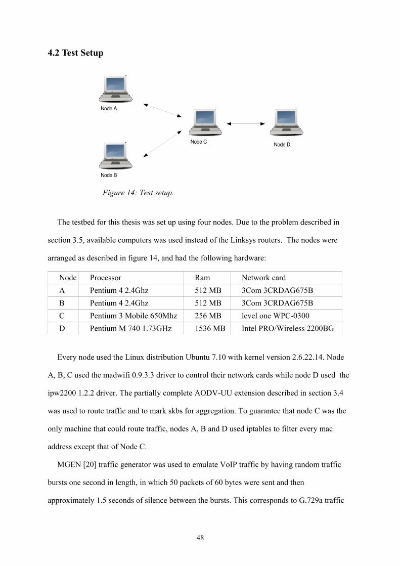
4.2 Test Setup
The testbed for this thesis was set up using four nodes. Due to the problem described in
section 3.5, available computers was used instead of the Linksys routers. The nodes were
arranged as described in figure 14, and had the following hardware:
Node Processor Ram Network card
A Pentium 4 2.4Ghz 512 MB 3Com 3CRDAG675B
B Pentium 4 2.4Ghz 512 MB 3Com 3CRDAG675B
C Pentium 3 Mobile 650Mhz 256 MB level one WPC-0300
D Pentium M 740 1.73GHz 1536 MB Intel PRO/Wireless 2200BG
Every node used the Linux distribution Ubuntu 7.10 with kernel version 2.6.22.14. Node
A, B, C used the madwifi 0.9.3.3 driver to control their network cards while node D used the
ipw2200 1.2.2 driver. The partially complete AODV-UU extension described in section 3.4
was used to route traffic and to mark skbs for aggregation. To guarantee that node C was the
only machine that could route traffic, nodes A, B and D used iptables to filter every mac
address except that of Node C.
MGEN [20] traffic generator was used to emulate VoIP traffic by having random traffic
bursts one second in length, in which 50 packets of 60 bytes were sent and then
approximately 1.5 seconds of silence between the bursts. This corresponds to G.729a traffic
48
Figure 14: Test setup.
Node A
Node B
Node C Node D
patterns with voice activity detection [19]. Traffic was created from node A to D, B to D and
the reverse directions. Node C was used to route the traffic. The data rate was set to 2Mbit/s.
Nodes A, B and D were set to capture incoming UDP packets on port 15000 and then start
transmission. After 180 seconds the test was terminated. This was repeated 20 times with an
increasing number of concurrent flows each time. One flow per link per test was used, which
means that the first time there was only 1 flow per link, and 20 flows per link at test 20. Since
there are four links (A-D, B-D, D-A, D-B) there were 4 flows in the first test, to a total of 80
injected flows in the last test.
A timeserver [21] was set up on node B, to allow node A and D to synchronize their clocks
before each test.
The aggregation module have some parameters that can be set. Timeout, which represents
how long a packet can be delayed before it must be sent, maximum size which represents
MTU and minimum size which is the minimum amount in bytes that need to have been
accumulated to cause the aggregation module to aggregate. Timeout was set to 5000, which is
5 milliseconds. Max was set to 1500 and min was set to 500, both in bytes.
The tool TRPR [22] was used to analyze the result provided by MGEN and produces
output files suitable for plotting.
49
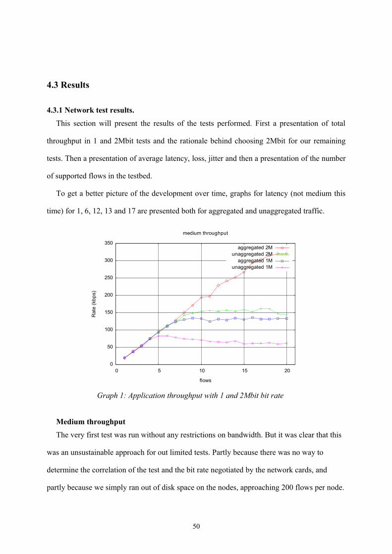
4.3 Results
4.3.1 Network test results.
This section will present the results of the tests performed. First a presentation of total
throughput in 1 and 2Mbit tests and the rationale behind choosing 2Mbit for our remaining
tests. Then a presentation of average latency, loss, jitter and then a presentation of the number
of supported flows in the testbed.
To get a better picture of the development over time, graphs for latency (not medium this
time) for 1, 6, 12, 13 and 17 are presented both for aggregated and unaggregated traffic.
Medium throughput
The very first test was run without any restrictions on bandwidth. But it was clear that this
was an unsustainable approach for out limited tests. Partly because there was no way to
determine the correlation of the test and the bit rate negotiated by the network cards, and
partly because we simply ran out of disk space on the nodes, approaching 200 flows per node.
50
Graph 1: Application throughput with 1 and 2Mbit bit rate
0
50
100
150
200
250
300
350
0 5 10 15 20
Rat
e (k
bp
s)
flows
medium throughput
aggregated 2Munaggregated 2M
aggregated 1Munaggregated 1M

To determine a bit rate that was as low as possible but would still yield good results over a
span of one to 20 flows per node, two tests was run at 1 and 2Mbit respectively and the
throughput was measured to determine the capacity of the test setup given the respective bit
rates.
As is visible in graph 1 the maximum capacity of the net is reached at 5 and 9 flows
respectively in the 1Mbit setup, and was determined to be insufficient to yield the best
possible results given a maximum of 20 flows per node.
In the 2Mbit test, as shown in graph 1, the maximum capacity is reached at 10 and 19
flows per node and was determined to be sufficient to yield good results given the maximum
of 20 flows per node.
It is interesting to see however that the relative difference between aggregated and
unaggregated traffic remains similar as the base rate of transmission changes.
What is shown in the graph is the average throughput of all four nodes combined and
plotted per test. The throughput is defined as the MGEN payload (32kbytes/packet) received
by each node. It is clearly visible that the throughput reaches a maximum capacity that is
supported by the network and that this capacity is fairly constant given network speed and
transmission method, aggregated or unaggregated. This could be interesting when considering
other potential uses for aggregation.
51
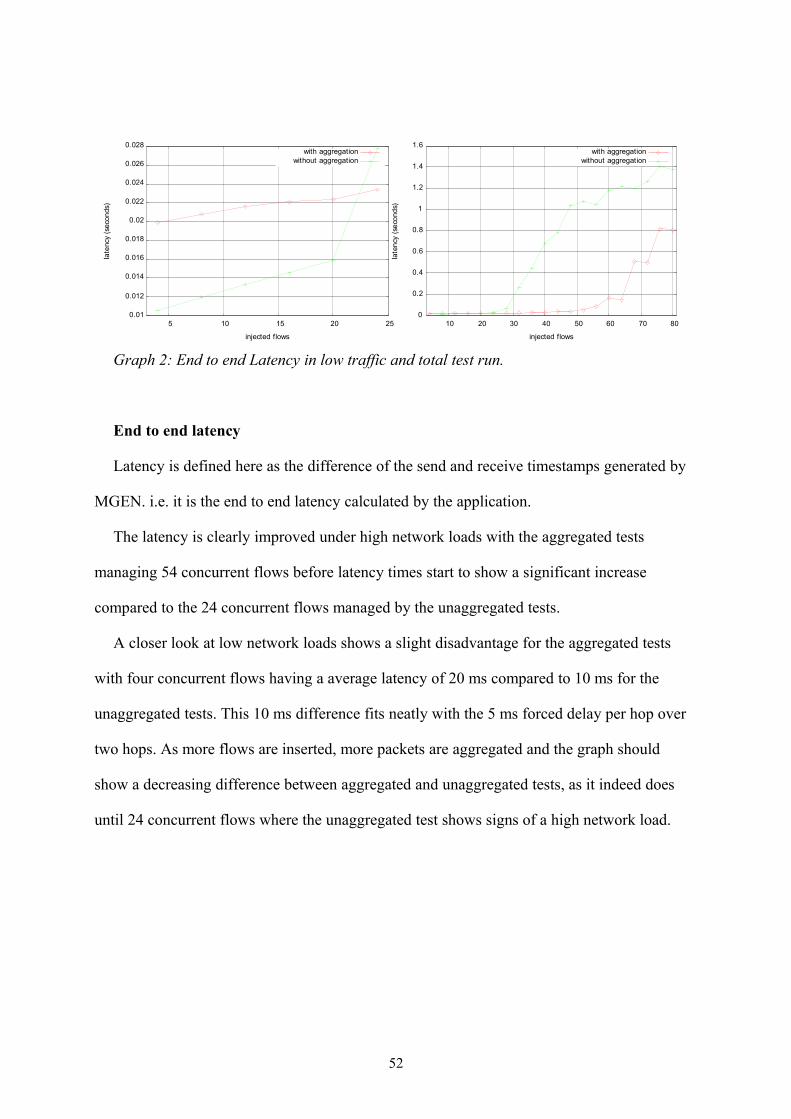
End to end latency
Latency is defined here as the difference of the send and receive timestamps generated by
MGEN. i.e. it is the end to end latency calculated by the application.
The latency is clearly improved under high network loads with the aggregated tests
managing 54 concurrent flows before latency times start to show a significant increase
compared to the 24 concurrent flows managed by the unaggregated tests.
A closer look at low network loads shows a slight disadvantage for the aggregated tests
with four concurrent flows having a average latency of 20 ms compared to 10 ms for the
unaggregated tests. This 10 ms difference fits neatly with the 5 ms forced delay per hop over
two hops. As more flows are inserted, more packets are aggregated and the graph should
show a decreasing difference between aggregated and unaggregated tests, as it indeed does
until 24 concurrent flows where the unaggregated test shows signs of a high network load.
52
Graph 2: End to end Latency in low traffic and total test run.
0.01
0.012
0.014
0.016
0.018
0.02
0.022
0.024
0.026
0.028
5 10 15 20 25
late
ncy
(sec
onds
)
injected flows
Average Latency
with aggregationwithout aggregation
0
0.2
0.4
0.6
0.8
1
1.2
1.4
1.6
10 20 30 40 50 60 70 80
late
ncy
(se
cond
s)
injected flows
Average Latency
with aggregationwithout aggregation
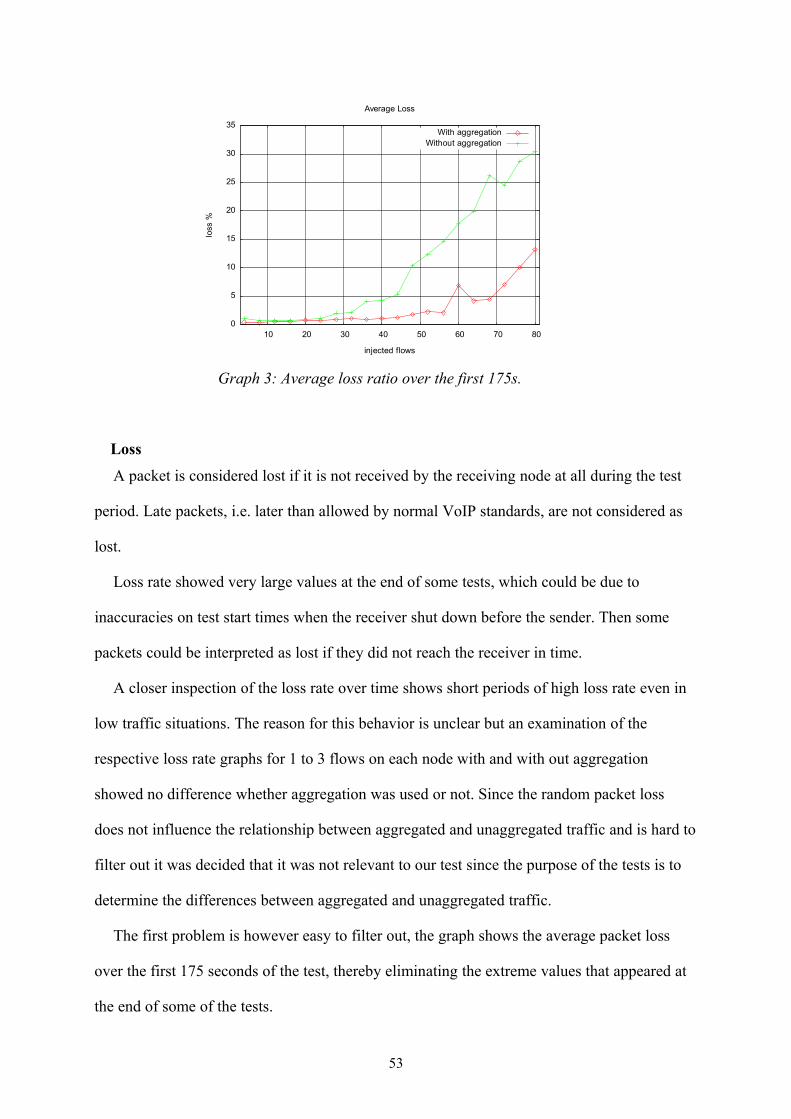
Loss
A packet is considered lost if it is not received by the receiving node at all during the test
period. Late packets, i.e. later than allowed by normal VoIP standards, are not considered as
lost.
Loss rate showed very large values at the end of some tests, which could be due to
inaccuracies on test start times when the receiver shut down before the sender. Then some
packets could be interpreted as lost if they did not reach the receiver in time.
A closer inspection of the loss rate over time shows short periods of high loss rate even in
low traffic situations. The reason for this behavior is unclear but an examination of the
respective loss rate graphs for 1 to 3 flows on each node with and with out aggregation
showed no difference whether aggregation was used or not. Since the random packet loss
does not influence the relationship between aggregated and unaggregated traffic and is hard to
filter out it was decided that it was not relevant to our test since the purpose of the tests is to
determine the differences between aggregated and unaggregated traffic.
The first problem is however easy to filter out, the graph shows the average packet loss
over the first 175 seconds of the test, thereby eliminating the extreme values that appeared at
the end of some of the tests.
53
Graph 3: Average loss ratio over the first 175s.
0
5
10
15
20
25
30
35
10 20 30 40 50 60 70 80
loss
%
injected flows
Average Loss
With aggregationWithout aggregation
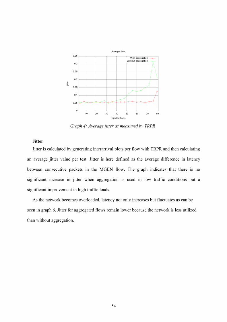
Jitter
Jitter is calculated by generating interarrival plots per flow with TRPR and then calculating
an average jitter value per test. Jitter is here defined as the average difference in latency
between consecutive packets in the MGEN flow. The graph indicates that there is no
significant increase in jitter when aggregation is used in low traffic conditions but a
significant improvement in high traffic loads.
As the network becomes overloaded, latency not only increases but fluctuates as can be
seen in graph 6. Jitter for aggregated flows remain lower because the network is less utilized
than without aggregation.
54
Graph 4: Average jitter as measured by TRPR
0
0.05
0.1
0.15
0.2
0.25
0.3
0.35
10 20 30 40 50 60 70 80
jitte
r
injected flows
Average Jitter
With aggregationWithout aggregation
Supported flows
A flow is considered supported if the average loss ratio is below 5% and the average
latency plus jitter is below 150 ms. These limits work under the assumption that the
distributions are fairly even, and the client implements a perfect jitter buffer. This is
unfortunately not true as is shown later when a closer inspection of the results over time is
presented, but it does provide a comparative metric which can be used to see the different
behavior of aggregated tests and unaggregated tests. The increase in supported flows is 135%
from 17 to 40 indicating a significant improvement. Further tests with other settings and real
VoIP communication should yield interesting results hopefully also provide better settings to
maximize the aggregation performance.
55
Graph 5: Supported flows in the testbed.
0
10
20
30
40
50
60
70
80
90
10 20 30 40 50 60 70 80
sup
por
ted
flo
ws
injected flows
supported flows
With aggregationWithout aggregation
Optimal support

Latency over time.
To better understand the behavior of the traffic and to see how sound the previous test
interpretations are it is interesting to study the latency as it changes over time, and keeping the
number of flows constant. Latency measures the time from start node to end node and
therefore gives a good picture of the conditions on the link.
For this purpose per packet latency is plotted for test number 1, 6, 12, 13 and 17 which
corresponds to 4, 24, 48, 52 and 68 injected flows. All graphs are from node D, i.e.hte
resrunting graphs show the flows arriving on node D, as it is considered representable for all
nodes and the actual values for each packet is of no interest. The tests were chosen for
different reasons.
• Test 1 was chosen to give a baseline for the behavior of low utilization situation.
• Test 6 was chosen because unaggregated traffic reaches a maximum value of 17
supported flows and the average delay times start to increase.
• Test 12 was chosen because the unaggregated traffic is bottoming out.
• Test 13 was chosen because aggregated traffic reaches a maximum value of 40
supported flows and the average delay times start to increase.
• Test 17 was chosen because aggregated traffic is bottoming out.
As is shown, the latency times in high load situations is not evenly distributed and shows
spikes. Since significant route instability was also occurring, observed by more lost and added
routes in the routing logs. In these situations we believe that most of these spikes can be
explained by a lost route. AODV-UU considers a link as down after five consecutive lost
HELLO messages from one host and deletes routes involving this link. The route is
reestablished once a new HELLO message is received from the host. Unfortunately there are
no routing log files saved from the tests so proving that routing instability is impossible in this
case.
56
AODV-UU can be easily configured for stable routes by increasing the lost route threshold
to a value larger than the test time in seconds, in this case over 180, or routing could be set up
with static routes. A test with stable routes could eliminate route instability as a source for
traffic degradation and could be useful for further evaluation of the aggregation. But
considering that this algorithm is designed for wireless mesh networks, dynamic routing is a
natural part of the environment and route stability is an important factor with the dynamic
routing protocols.
57
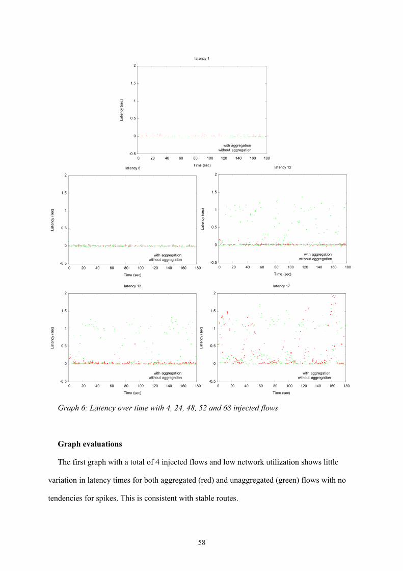
Graph evaluations
The first graph with a total of 4 injected flows and low network utilization shows little
variation in latency times for both aggregated (red) and unaggregated (green) flows with no
tendencies for spikes. This is consistent with stable routes.
58
Graph 6: Latency over time with 4, 24, 48, 52 and 68 injected flows
-0.5
0
0.5
1
1.5
2
0 20 40 60 80 100 120 140 160 180
Lat
enc
y (s
ec)
Time (sec)
latency 1
with aggregationwithout aggregation
-0.5
0
0.5
1
1.5
2
0 20 40 60 80 100 120 140 160 180
Late
ncy
(sec
)
Time (sec)
latency 6
with aggregationwithout aggregation
-0.5
0
0.5
1
1.5
2
0 20 40 60 80 100 120 140 160 180
Late
ncy
(sec
)
Time (sec)
latency 12
with aggregationwithout aggregation
-0.5
0
0.5
1
1.5
2
0 20 40 60 80 100 120 140 160 180
Late
ncy
(sec
)
Time (sec)
latency 13
with aggregationwithout aggregation
-0.5
0
0.5
1
1.5
2
0 20 40 60 80 100 120 140 160 180
Lat
enc
y (s
ec)
Time (sec)
latency 17
with aggregationwithout aggregation
The second graph with a total of 24 injected flows, is the test with the most supported
unaggregated flows (17). There are some spikes consistent with the lost route that would have
interrupted voice communication for a short time but did not influence the average value too
much. Aggregated traffic still behaves in a good manner with only one small spike.
The third graph with a total of 48 injected flows, which is the test where the unaggregated
test reached 0 supported flows and the network is completely overloaded. On inspection route
stability was very poor at this point and the latency times varies between 0.1 to 1.5 seconds.
Aggregated traffic, however, still behaves in a fairly good manner with some occasional
spikes similar to the situation for unaggregated traffic and 24 injected flows.
The fourth graph with a total of 52 injected flows shows a similar behavior to graph 3. This
is the test with the most supported aggregated flows (40). Compared to graph 3 the only
discernible difference is that the spikes for the aggregated traffic is a bit more pronounced.
The fifth graph with a total of 68 injected flows shows a completely overloaded network.
This is the test where supported aggregated flows reached 0. The aggregated traffic starts to
resemble the unaggregated traffic with one interesting difference; where unaggregated traffic
seems to frequently jump between high and low latency with relatively short durations of the
spikes, aggregated traffic seems to loose route with a lower frequency but the height (max
latency) and duration of the individual spike is increased. This behavior could be explained by
a higher processor load on the router when processing the aggregated backlog once the route
is reestablished.
In conclusion to this latency evaluation, the network s stable in low traffic situations but
once the peak in supported flows is reached the difference in latency within flows are
indicating that the number of supported flows in reality lower, (close to the expected sharp
drop off expected). But even if the actual numbers of supported flows in higher utilization
scenarios is not to be too trusted the difference in what is a high utilization of the network
59
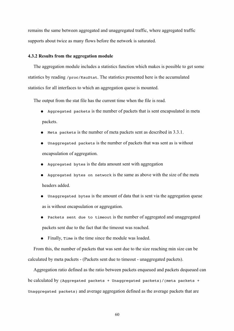
remains the same between aggregated and unaggregated traffic, where aggregated traffic
supports about twice as many flows before the network is saturated.
4.3.2 Results from the aggregation module
The aggregation module includes a statistics function which makes is possible to get some
statistics by reading /proc/KauStat. The statistics presented here is the accumulated
statistics for all interfaces to which an aggregation queue is mounted.
The output from the stat file has the current time when the file is read.
● Aggregated packets is the number of packets that is sent encapsulated in meta
packets.
● Meta packets is the number of meta packets sent as described in 3.3.1.
● Unaggregated packets is the number of packets that was sent as is without
encapsulation of aggregation.
● Aggregated bytes is the data amount sent with aggregation
● Aggregated bytes on network is the same as above with the size of the meta
headers added.
● Unaggregated bytes is the amount of data that is sent via the aggregation queue
as is without encapsulation or aggregation.
● Packets sent due to timeout is the number of aggregated and unaggregated
packets sent due to the fact that the timeout was reached.
● Finally, Time is the time since the module was loaded.
From this, the number of packets that was sent due to the size reaching min size can be
calculated by meta packets - (Packets sent due to timeout - unaggregated packets).
Aggregation ratio defined as the ratio between packets enqueued and packets dequeued can
be calculated by (Aggregated packets + Unaggregated packets)/(meta packets +
Unaggregated packets) and average aggregation defined as the average packets that are
60
aggregated into one meta packet can be calculated by Aggregated packets / meta
packets.
The module behavior can be examined by manipulating the data from these statistics files.
Graph 7 show the average aggregation and aggregation ratio. It indicates that the
aggregation ratio is a linear function, proportional to the number of concurrent flows in the
link. It also seems to indicate that average aggregation will eventually be equal to the
aggregation ratio as the occurrence of unaggregated packets approaches zero as the number of
flows increase. Another reasonable assumption although not evident in the graphs is that both
curves will level out at max frame size / unaggregated frame size due to the fact that no more
packets can be aggregated into one meta packet. To prove this a higher bandwidth and more
flows are required.
Graph 8 show the average number of packets per flow on the network and illustrates some
interesting things in the modules´ behavior.
The number of packets generated by MGEN per flow during the tests has a random
variation, but this variation is small compared to the total number of packets per flow and an
average over all flows results in an even smaller variation. In this context the variation can be
considered to small to impact the packet count on the network in any significant way. It is
interesting to see that the average number of packets per flow on the network (red) is greatly
61
Graph 8: Average packets sent per flowGraph 7: Aggregation ratio
1
1.5
2
2.5
3
3.5
4
4.5
5
5.5
2 4 6 8 10 12 14 16 18 20
agg
reg
atio
n r
atio
test
Average aggregation
Average aggregationAggregation ratio
0
1000
2000
3000
4000
5000
6000
7000
10 20 30 40 50 60 70 80
nu
mb
er o
f p
acke
ts
flows
average packets sent per flow
totalunaggregated
total meta packetstimeout
size
reduced as the number of concurrent flows on the network increase. The unaggregated traffic
is approaching zero and the number of aggregated packets (blue) is increasing up to a point,
around 24 concurrent flows on the network. After that the increase of aggregated traffic
compared to unaggregated traffic on the network is offset by the average aggregation
increasing the number of packets per meta packet.
It can also be seen that as the number of concurrent flows increase, the number of meta
packets sent before the timeout because the min size has been reached is increased.
4.4 Summary
The tests show that in a test setup as described in 4.2 with the bit rate limited to 2Mbit, the
aggregation scheme does indeed perform as expected.
Latency and the number of supported flows is consistent with the predicted results.
Another interesting result is the latency over time, which is probably influenced by route
instability. This will have to be proven in further tests. But it does indicate that aggregation
can increase route stability in wireless mesh networks simply by lowering network utilization.
The results from the module itself shows the behavior with a low bit rate, but some
interesting tendencies can just be hinted at as the load increases. The tendency to send packets
before the forced delay due to a large enough size needs higher bandwidth tests in order to be
properly shown.
62
5 Conclusions
In this chapter a general summary of the project as a whole is presented in 5.1.Open issues
regarding the implementation and work that we were for various reasons unable to finish is
discussed in 5.2 Questions and ideas about future work that have been raised during the
course of this project is discussed in 5.3. Other applications for the implementation are
discussed in 5.4, and a final summary and conclusions drawn from this thesis are presented in
5.5.
5.1 General Summary
The primary goal of the project, which was to implement the aggregation in Linux, was
met. With the results from the tests showing the viability of the implementation. Lack of time
and unexpected driver issues prevented the implementation of the secondary goals. Dynamic
aggregation is however possible if and when the AODV-UU or another similar routing
protocol due to the passing of the frame size as part of the firewall mark field. The code is
well commented since it is thought of as a base for further development, and porting to other
kernels by a third person should be as easy as possible. Hopefully future use of this
implementation will prove useful for further research in the field of wireless networks.
5.2 Open Issues
There are some issues that are still outstanding and improvements that we did not have
time to address.
The aggregation qdisc is supposed to be able to be mounted as a sub queue to any classful
qdisc such as cbq, a popular queuing discipline in the Linux kernel. Unfortunately it can only
63

be mounted on simplerr, partly because no tc module specific to the aggregation qdisc is
written. This is however not very difficult to implement. The other more serious reason is the
calculation of statistics such as backlog and queue length used by other qdiscs. This is not
compatible with aggregation since number and length of packets enqueued is not equal to
dequeued. Simplerr solves this by reading the aggregation statistics directly from the
aggregation qdisc, but it creates a dependency between aggregation and simplerr.
Another issue is related to dynamic aggregation. While it is possible to send the max frame
size with the firewall mark field, the minimum aggregation size is set statically by tc.
Unfortunately tests have proven that it is most often the min size that determines the actual
frame size. To make the aggregation module fully support dynamic aggregation min size has
to be redefined as a fixed size smaller than max size, or as a defined fraction or percentage of
max size.
The unfortunate problems with the extensions to AODV-UU does present the issue of
reported signal strength from the different drivers but the partial implementation presented in
the thesis shows that a full implementation is possible given some restrictions on the drivers
used or by using another approach to calculate the frame size.
As to the implementation on the Linksys routers, the main issue is of course the driver to
the broadcom chipset. This issue can be solved by either porting the modules to the 2.4
kernel. Another approach is to further develop the b43 driver present in the later 2.6 versions
of the kernel. While this approach is a project all in itself it would enable the use of dynamic
aggregation since it would be possible to access parts of the chipset that is impossible with the
binary driver.
The last open issue to be discussed here is the matter or route stability and the impact on
the tests. If the assumptions that route stability is the cause of the spikes in the latency graphs
proves to be correct, a discussion on the possible impact on the tests and real world
64
performance is desired. But it would also show that the use of aggregation can also increase
route stability due to lower network utilization.
5.3 Future Work
The tests clearly show potential for increased performance of wireless networks by
aggregating packets to reduce network overhead. To maximize the advantage of aggregation,
the effect of timeout values and packet sizes have to be further researched. Porting of the
modules to other kernel versions, including 2.4 version for greater versatility of application
platforms, would of course be interesting. Such a porting to IPv6 which should be possible
without too much hassle.
The networking group at Karlstads University currently integrates the aggregation module
in the platform which is developed in the DAIDALOS project [23]. The aggregation module
is an optional part on the mobile terminals and the mobile gateways to enhance the VoIP
capacity. The Daidalos platform is based on Ubuntu 6.06. Thus, the aggregation module had
to be backported to Kernel version 2.6.16, which is used in this Ubuntu version. By April
2008 a first working version for the Daidalos platform is available. Future activities include
the use of IPv6 instead of IPv4 and the dynamic control of the min and the timeout parameters
be the DAIDALOS QoS controller component.
5.4 Other Applications
The use of aggregation is clearly not limited to VoIP communication, but could be used for
any type of network communication where per link frame size optimization would be
beneficial.
65
5.5 Summary and Conclusions
This thesis presents a implementation of packet aggregation in a Linux environment.
Even though not all goals were met, the primary goals of implementing the aggregation
scheme in the Linux kernel were fulfilled. And while the secondary goals were not met, there
has been some progress made towards finishing them as well, and hopefully this work will
still prove beneficial to anyone who wishes to further develop aggregation as a concept.
Tests show that the aggregation modules behave as expected and the effect on the network
shows that this implementation can be a valuable tool for future research into the field of
wireless networks.
66
References
[1] Dely Peter, Adaptive Aggregation of Voice over IP in Wireless Mesh Networks, Karlstad University, 200708.
[2] Akyildiz I.F., Wang X., Wang W., Wireless Mesh Networks: a survey, Computer Networks, 2005. 47(4): p 445 – 487.
[3] Christian Benvenuti, Understanding Linux Network Internals, 2006, O'Reilly, ISBN 0-596-00255-6.
[4] Xiuchao, W., Simulate 802.11b channel within ns2. 2004, National University ofSingapore: Singapore.
[5] NIST/SEMATECH, e-Handbook of Statistical Methods. 2006 [cited 20080326]; URL:
http://www.itl.nist.gov/div898/handbook/pmc/section4/pmc431.htm.
[6] Rusty Russell and Harald Welte, Linux netfilter Hacking HOWTO [cited 20080416];
URL: http://www.netfilter.org/documentation/HOWTO//netfilter-hacking-HOWTO.html
[7]Linux source 2.6.22 /include/linux/netfilter_ipv4.h
[8] Linux Advanced Routing & Traffic Control, TC man page,[cited ,20080416]; URL: http://
lartc.org/manpages/tc.txt
[9] Department of Computer Science University of California Santa Barbara, AODV,[cited
20080416]; URL: http://moment.cs.ucsb.edu/AODV/
[10] Department of Computer Science Uppsala University, AODV-UU [cited 20080416];
URL: http://core.it.uu.se/core/index.php/AODV-UU
[11] IETF, RFC 3692 IP protocol field, [cited 20080324 ]; URL:
http://tools.ietf.org/html/rfc3692#section-2.1,
[12] The Linux Foundation, Net: Iproute2, [cited 20080324]; URL: http://www.linux-
foundation.org/en/Net:Iproute2
[13] Linux Documentation, modprobe – Linux man page,[cited 20080416]; URL:
http://linux.die.net/man/8/modprobe
[14] Linux Documentation, insmod – Linux man page,[cited 20080416]; URL:
http://linux.die.net/man/8/insmod
[15] Jean Tourrilhes, Wireless tools for Linux,[cited 20080416]; URL:
http://www.hpl.hp.com/personal/Jean_Tourrilhes/Linux/Tools.html
[16] Linux Documentation, ioctl – Linux man page, [cited 20080416]; URL:
http://linux.die.net/man/2/ioctl
67
[17] K. Kyungtae and H. Sangjin, "VoMESH: voice over wireless mesh networks," in Proc. of
IEEE Wireless Communications and Networking Conference Las Vegas, NV, USA, 2006, pp.
193-8.
[18] Linksys, [cited 20080509]; URL: http://www-se.linksys.com
[19] International Telecommunication Union, “ITU-T Recommendation P.59 - Artificial
conversational speech”. 1993
[20] Naval research laboratory, Multi-Generator (MGEN), [cited 20080324]; URL:
http://cs.itd.nrl.navy.mil/work/mgen/,
[21] L. Frank Baum , Network Time Protocol (NTP) deamon, [cited 20080326]; URL: http://
www.cis.udel.edu/~mills/ntp/html/ntpd.html ,
[22] Naval research Laboratory, trpr 2.0b1 User's Guide,[cited 20080326]; URL:
http://pf.itd.nrl.navy.mil/protools/trpr.html ,
[23] FP6 IST Integrated Project DAIDALOS,[cited 20080525]; URL: http://www.ist-
daidalos.org/
[24]Ashish Jain, Marco Gruteser, Mike Neufeld, Dirk Grunwald, “Benefits of Packet
Aggregation in Ad-Hoc Wireless Network”, Department of Computer Science , University of
Colorado at Boulder , August 2003.
[25] Sangkil Jung, Sangjin Hong, Kyungtae Kim, Junghoon Jee, Eunah Kim, “Voice
Transmission Enhancing Model on Wireless Mesh Networks ”
[26] Bert Hubert, “Linux Advanced Routing & Traffic Control HOWTO” , 20031029
68


![Index [assets.cambridge.org]assets.cambridge.org/97805218/60253/index/9780521860253_index… · aggregation. See bubble, aggregation; particle, aggregation; particle, concentration](https://img.pdfslide.us/doc/110x75/60634dbbe29a93467d378f87/index-aggregation-see-bubble-aggregation-particle-aggregation-particle.jpg)