Package ‘WebPower’ - cran.r-project.org · MRT3 Example Data For MRT With 3 Arms Description •ID. The identiﬁcation number of the subjects. •cluster. The cluster number

Package ‘WebPower’April 16, 2018

Title Basic and Advanced Statistical Power Analysis

Version 0.5

Date 2018-04-01

Author Zhiyong Zhang [aut, cre],Yujiao Mai [aut],Miao Yang [ctb]

Maintainer Zhiyong Zhang <[email protected]>

Depends R (>= 3.2.5), MASS, stats, grDevices, graphics, lme4, lavaan,parallel, PearsonDS

License GPL (>= 3)

Description This is a collection of tools for conducting both basic and advanced statistical power anal-ysis including correlation, proportion, t-test, one-way ANOVA, two-way ANOVA, linear regres-sion, logistic regression, Poisson regression, mediation analysis, longitudinal data analysis, struc-tural equation modeling and multilevel modeling. It also serves as the engine for conduct-ing power analysis online at <https://webpower.psychstat.org>.

URL https://webpower.psychstat.org

Encoding UTF-8

LazyLoad yes

LazyData yes

NeedsCompilation no

Repository CRAN

Date/Publication 2018-04-16 09:08:06 UTC

R topics documented:WebPower-package . . . . . . . . . . . . . . . . . . . . . . . . . . . . . . . . . . . . . 2CRT2 . . . . . . . . . . . . . . . . . . . . . . . . . . . . . . . . . . . . . . . . . . . . 3CRT3 . . . . . . . . . . . . . . . . . . . . . . . . . . . . . . . . . . . . . . . . . . . . 4estCRT2arm . . . . . . . . . . . . . . . . . . . . . . . . . . . . . . . . . . . . . . . . . 5MRT2 . . . . . . . . . . . . . . . . . . . . . . . . . . . . . . . . . . . . . . . . . . . . 5MRT3 . . . . . . . . . . . . . . . . . . . . . . . . . . . . . . . . . . . . . . . . . . . . 6

1

https://webpower.psychstat.org

2 WebPower-package

nuniroot . . . . . . . . . . . . . . . . . . . . . . . . . . . . . . . . . . . . . . . . . . . 7plot.lcs.power . . . . . . . . . . . . . . . . . . . . . . . . . . . . . . . . . . . . . . . . 8plot.webpower . . . . . . . . . . . . . . . . . . . . . . . . . . . . . . . . . . . . . . . . 8print.webpower . . . . . . . . . . . . . . . . . . . . . . . . . . . . . . . . . . . . . . . 9summary.power . . . . . . . . . . . . . . . . . . . . . . . . . . . . . . . . . . . . . . . 10wp.anova . . . . . . . . . . . . . . . . . . . . . . . . . . . . . . . . . . . . . . . . . . 10wp.anova.binary . . . . . . . . . . . . . . . . . . . . . . . . . . . . . . . . . . . . . . . 13wp.anova.count . . . . . . . . . . . . . . . . . . . . . . . . . . . . . . . . . . . . . . . 15wp.blcsm . . . . . . . . . . . . . . . . . . . . . . . . . . . . . . . . . . . . . . . . . . 17wp.correlation . . . . . . . . . . . . . . . . . . . . . . . . . . . . . . . . . . . . . . . . 20wp.crt2arm . . . . . . . . . . . . . . . . . . . . . . . . . . . . . . . . . . . . . . . . . 23wp.crt3arm . . . . . . . . . . . . . . . . . . . . . . . . . . . . . . . . . . . . . . . . . 25wp.effect.CRT2arm . . . . . . . . . . . . . . . . . . . . . . . . . . . . . . . . . . . . . 27wp.effect.CRT3arm . . . . . . . . . . . . . . . . . . . . . . . . . . . . . . . . . . . . . 28wp.effect.MRT2arm . . . . . . . . . . . . . . . . . . . . . . . . . . . . . . . . . . . . . 29wp.effect.MRT3arm . . . . . . . . . . . . . . . . . . . . . . . . . . . . . . . . . . . . . 30wp.kanova . . . . . . . . . . . . . . . . . . . . . . . . . . . . . . . . . . . . . . . . . . 32wp.lcsm . . . . . . . . . . . . . . . . . . . . . . . . . . . . . . . . . . . . . . . . . . . 33wp.logistic . . . . . . . . . . . . . . . . . . . . . . . . . . . . . . . . . . . . . . . . . . 35wp.mc.sem.basic . . . . . . . . . . . . . . . . . . . . . . . . . . . . . . . . . . . . . . 37wp.mc.sem.boot . . . . . . . . . . . . . . . . . . . . . . . . . . . . . . . . . . . . . . . 40wp.mc.sem.power.curve . . . . . . . . . . . . . . . . . . . . . . . . . . . . . . . . . . . 43wp.mc.t . . . . . . . . . . . . . . . . . . . . . . . . . . . . . . . . . . . . . . . . . . . 45wp.mediation . . . . . . . . . . . . . . . . . . . . . . . . . . . . . . . . . . . . . . . . 47wp.mmrm . . . . . . . . . . . . . . . . . . . . . . . . . . . . . . . . . . . . . . . . . . 49wp.mrt2arm . . . . . . . . . . . . . . . . . . . . . . . . . . . . . . . . . . . . . . . . . 50wp.mrt3arm . . . . . . . . . . . . . . . . . . . . . . . . . . . . . . . . . . . . . . . . . 52wp.poisson . . . . . . . . . . . . . . . . . . . . . . . . . . . . . . . . . . . . . . . . . 55wp.popPar . . . . . . . . . . . . . . . . . . . . . . . . . . . . . . . . . . . . . . . . . . 57wp.prop . . . . . . . . . . . . . . . . . . . . . . . . . . . . . . . . . . . . . . . . . . . 57wp.regression . . . . . . . . . . . . . . . . . . . . . . . . . . . . . . . . . . . . . . . . 59wp.rmanova . . . . . . . . . . . . . . . . . . . . . . . . . . . . . . . . . . . . . . . . . 62wp.sem.chisq . . . . . . . . . . . . . . . . . . . . . . . . . . . . . . . . . . . . . . . . 64wp.sem.rmsea . . . . . . . . . . . . . . . . . . . . . . . . . . . . . . . . . . . . . . . . 66wp.t . . . . . . . . . . . . . . . . . . . . . . . . . . . . . . . . . . . . . . . . . . . . . 68

Index 72

WebPower-package Basic and Advanced Statistical Power Analysis

Description

This is a collection of tools for conducting both basic and advanced statistical power analysis includ-ing correlation, proportion, t-test, one-way ANOVA, two-way ANOVA, linear regression, logisticregression, Poisson regression, mediation analysis, longitudinal data analysis, structural equationmodeling and multilevel modeling. It also serves as the engineer for conducting power analysisonline at https://webpower.psychstat.org.

CRT2 3

Details

This is a collection of tools for conducting both basic and advanced statistical power analysis includ-ing correlation, proportion, t-test, one-way ANOVA, two-way ANOVA, linear regression, logisticregression, Poisson regression, mediation analysis, longitudinal data analysis, structural equationmodeling and multilevel modeling. It also serves as the engineer for conducting power analysisonline at https://webpower.psychstat.org.

References

Zhang, Z., & Yuan, K.-H. (2018). Practical Statistical Power Analysis Using Webpower and R(Eds). Granger, IN: ISDSA Press.

CRT2 Example Data For CRT With 2 Arms

Description

• ID. The identification number of the subjects.

• cluster. The cluster number.

• score. The score of the subject.

• group. The group number.

Usage

CRT2

Format

An object of class data.frame with 8 rows and 4 columns.

Examples

# ID cluster score group# 1 1 6 0# 2 1 2 0# 3 2 6 1# 4 2 5 1# 5 3 1 0# 6 3 4 0# 7 4 6 1# 8 4 4 1

4 CRT3

CRT3 Example Data For CRT With 3 Arms

Description





Usage

CRT3

Format


Examples

# id cluster score group# 1 1 1.93 0# 2 1 1.51 0# 3 1 2.13 0# 4 1 2.96 0# 5 1 3.84 0# 6 2 3.36 1# 7 2 3.13 1# 8 2 1.71 1# 9 2 3.1 1# 10 2 2.53 1# 11 3 2.01 2# 12 3 4.73 2# 13 3 3.34 2# 14 3 0.11 2# 15 3 3.6 2# 16 4 2 0# 17 4 1.99 0# 18 4 1.89 0# 19 4 2.25 0# 20 4 1.83 0# 21 5 3.03 1# 22 5 2.08 1# 23 5 1.5 1# 24 5 3.18 1# 25 5 1.92 1# 26 6 3.49 2# 27 6 3.08 2# 28 6 4.54 2

estCRT2arm 5

# 29 6 2.34 2# 30 6 4.33 2

estCRT2arm Estimate multilevel effect size from data

Description

Estimate multilevel effect size from data

Usage

estCRT2arm(file)estCRT3arm(file)estMRT2arm(file)estMRT3arm(file)

Arguments

file a data file

MRT2 Example Data For MRT With 2 Arms

Description





Usage

MRT2

Format


6 MRT3

Examples

#Example data for MRT with 2 arms# id cluster score group# 1 1 6 0# 2 1 2 0# 3 1 3 1# 4 1 3 1# 5 2 6 0# 6 2 10 0# 7 2 7 1# 8 2 6 1# 9 3 6 0# 10 3 5 0# 11 3 4 1# 12 3 4 1# 13 4 1 0# 14 4 8 0# 15 4 10 1# 16 4 -2 1

MRT3 Example Data For MRT With 3 Arms

Description





Usage

MRT3

Format


Examples

# id cluster score group# 1 1 2 0# 2 1 3 0# 3 1 2 1# 4 1 0 1# 5 1 3 2# 6 1 2 2# 7 2 1 0

nuniroot 7

# 8 2 4 0# 9 2 2 1# 10 2 3 1# 11 2 3 2# 12 2 1 2# 13 3 1 0# 14 3 4 0# 15 3 1 1# 16 3 1 1# 17 3 2 2# 18 3 0 2# 19 4 4 0# 20 4 3 0# 21 4 1 1# 22 4 3 1# 23 4 3 2# 24 4 3 2

nuniroot Sove An Single Equation

Description

The function searches in an interval for a root (i.e., zero) of the function f with respect to its firstargument. The argument interval is for the input of x, the corresponding outcome interval will beused as the interval to be searched in.

Usage

nuniroot(f, interval, maxlength = 100)

Arguments

f Function for which the root is sought.

interval A vector containing the end-points of the interval to be searched for the root.

maxlength The number of vaulue points in the interval to be searched. It is 100 by default.

Value

A list with at least four components: root and f.root give the location of the root and the value ofthe function evaluated at that point. iter and estim.prec give the number of iterations used and anapproximate estimated precision for root. (If the root occurs at one of the endpoints, the estimatedprecision is NA.)

8 plot.webpower

Examples

f <- function(x) 1+x-0.5*x^2interval <- c(-3,-2,1,2,6)nuniroot(f,interval)

plot.lcs.power Plot the power curve for Latent Change Score Models

Description

This function is used to plot the power analysis results for Latent Change Score Models.

Usage

## S3 method for class 'lcs.power'plot(x, parameter, ...)

Arguments

x Data to plot.

parameter Parameters for features of the plot.

... Extra arguments. It is not required.

References

Zhang, Z., & Liu, H. (2018). Sample Size and Measurement Occasion Planning for Latent ChangeScore Models through Monte Carlo Simulation. In E. Ferrer, S. M. Boker, and K. J. Grimm (Eds.)Advances in Longitudinal Models for Multivariate Psychology: A Festschrift for Jack McArdle.


plot.webpower To plot Statistical Power Curve

Description

This function is used to plot the power curves generated by webpower.

Usage

## S3 method for class 'webpower'plot(x, xvar = NULL, yvar = NULL, xlab = NULL,ylab = NULL, ...)

print.webpower 9

Arguments

x Objects of power analysis.xvar The variable name used as the x (horizontal) axis. It is not required.yvar The variable name used as the y (vertical) axis. It is not required.xlab The label for the x axis. It is not required.ylab The label for the y axis. It is not required.... Extra arguments. It is not required.

Value

The plot.

Examples

res <- wp.correlation(n=50,r=0.3, alternative="two.sided")plot(res)

print.webpower To Print Statistical Power Analysis Results

Description

This function is used to summary the power analysis results.

Usage

## S3 method for class 'webpower'print(x, ...)

Arguments

x Object of power analysis. It is an object returned by a webpower function suchas wp.anova().


Value

The printing of the input object of power analysis.

Examples

res <- wp.correlation(n=50,r=0.3, alternative="two.sided")print(res)

10 wp.anova

summary.power Summary Statistical Power Analysis Results

Description

This function is used to summary the power analysis results.

Usage

## S3 method for class 'power'summary(object, ...)

Arguments

object Object of power analysis. It is an object returned by a webpower function forSEM based on Monte Carlo methods with class = ’power’.


Value

The summary of the input object of power analysis.

wp.anova Statistical Power Analysis for One-way ANOVA

Description

One-way analysis of variance (one-way ANOVA) is a technique used to compare means of two ormore groups (e.g., Maxwell & Delaney, 2003 ). The ANOVA tests the null hypothesis that samplesin two or more groups are drawn from populations with the same mean values. The ANOVAanalysis typically produces an F-statistic, the ratio of the bewteen-group variance to the within-group variance.

Usage

wp.anova(k = NULL, n = NULL, f = NULL, alpha = 0.05, power = NULL,type = c("overall", "two.sided", "greater", "less"))

wp.anova 11

Arguments

k Number of groups.

n Sample size.

f Effect size. We use the statistic f as the measure of effect size for one-wayANOVA as in Cohen (1988). Cohen defined the size of effect as: small 0.1,medium 0.25, and large 0.4.

alpha Significance level chosed for the test. It equals 0.05 by default.

power Statistical power.

type Type of test ("overall" or "two.sided" or "greater" or "less"). The defaultis "two.sided". The option "overall" is for the overall test of anova; "two.sided"is for a contrast anova; "greater" is testing the between-group vairance greaterthan the within-group, while "less" is vis versus.

Value

An object of the power analysis.

References

Cohen, J. (1988). Statistical power analysis for the behavioral sciences (2nd Ed). Hillsdale, NJ:Lawrence Erlbaum Associates.

Maxwell, S. E., & Delaney, H. D. (2004). Designing experiments and analyzing data: A modelcomparison perspective (Vol. 1). Psychology Press.


Examples

#To calculate the statistical power for the overall test of one-way ANOVA:wp.anova(f=0.25,k=4, n=100, alpha=0.05)# Power for One-way ANOVA## k n f alpha power# 4 100 0.25 0.05 0.5181755## NOTE: n is the total sample size (overall)# URL: http://psychstat.org/anova

#To calculate the power curve with a sequence of sample sizes:res <- wp.anova(f=0.25, k=4, n=seq(100,200,10), alpha=0.05)res# Power for One-way ANOVA## k n f alpha power# 4 100 0.25 0.05 0.5181755# 4 110 0.25 0.05 0.5636701# 4 120 0.25 0.05 0.6065228# 4 130 0.25 0.05 0.6465721

12 wp.anova

# 4 140 0.25 0.05 0.6837365# 4 150 0.25 0.05 0.7180010# 4 160 0.25 0.05 0.7494045# 4 170 0.25 0.05 0.7780286# 4 180 0.25 0.05 0.8039869# 4 190 0.25 0.05 0.8274169# 4 200 0.25 0.05 0.8484718## NOTE: n is the total sample size (overall)# URL: http://psychstat.org/anova

#To plot the power curve:plot(res, type='b')

#To estimate the sample size with a given power:wp.anova(f=0.25,k=4, n=NULL, alpha=0.05, power=0.8)# Power for One-way ANOVA## k n f alpha power# 4 178.3971 0.25 0.05 0.8## NOTE: n is the total sample size (overall)# URL: http://psychstat.org/anova

#To estimate the minimum detectable effect size with a given power:wp.anova(f=NULL,k=4, n=100, alpha=0.05, power=0.8)# Power for One-way ANOVA## k n f alpha power# 4 100 0.3369881 0.05 0.8## NOTE: n is the total sample size (overall)# URL: http://psychstat.org/anova

#To conduct power analysis for a contrast one-way ANOVA:wp.anova(f=0.25,k=4, n=100, alpha=0.05, type='two.sided')# Power for One-way ANOVA## k n f alpha power# 4 100 0.25 0.05 0.6967142## NOTE: n is the total sample size (contrast, two.sided)# URL: http://psychstat.org/anova

#To calculate the power curve with a sequence of sample sizes:res <- wp.anova(f=seq(0.1, 0.8, 0.1), k=4, n=100, alpha=0.05)res# Power for One-way ANOVA## k n f alpha power# 4 100 0.1 0.05 0.1128198# 4 100 0.2 0.05 0.3452612# 4 100 0.3 0.05 0.6915962

wp.anova.binary 13

# 4 100 0.4 0.05 0.9235525# 4 100 0.5 0.05 0.9911867# 4 100 0.6 0.05 0.9995595# 4 100 0.7 0.05 0.9999908# 4 100 0.8 0.05 0.9999999## NOTE: n is the total sample size (overall)# URL: http://psychstat.org/anova

wp.anova.binary Statistical Power Analysis for One-way ANOVA with Binary Data

Description

The power analysis procedure for one-way ANOVA with binary data is introduced by Mai andZhang (2017). One-way ANOVA with binary data is used for comparing means of three or moregroups of binary data. Its outcome variable is supposed to follow Bernoulli distribution. And itsoverall test uses a likelihood ratio test statistics.

Usage

wp.anova.binary(k = NULL, n = NULL, V = NULL, alpha = 0.05,power = NULL)

Arguments

k Number of groups.

n Sample size.

V Effect size. See the research by Mai and Zhang (2017) for details.



Value


References

Mai, Y., & Zhang, Z. (2017). Statistical Power Analysis for Comparing Means with Binary orCount Data Based on Analogous ANOVA. In L. A. van der Ark, M. Wiberg, S. A. Culpepper,J. A. Douglas, & W.-C. Wang (Eds.), Quantitative Psychology - The 81st Annual Meeting of thePsychometric Society, Asheville, North Carolina, 2016: Springer.


14 wp.anova.binary

Examples

#To calculate the statistical power for one-way ANOVA (overall test) with binary data:wp.anova.binary(k=4,n=100,V=0.15,alpha=0.05)# One-way Analogous ANOVA with Binary Data## k n V alpha power# 4 100 0.15 0.05 0.5723443## NOTE: n is the total sample size# URL: http://psychstat.org/anovabinary

#To generate a power curve given a sequence of sample sizes:res <- wp.anova.binary(k=4,n=seq(100,200,10),V=0.15,alpha=0.05,power=NULL)res# One-way Analogous ANOVA with Binary Data## k n V alpha power# 4 100 0.15 0.05 0.5723443# 4 110 0.15 0.05 0.6179014# 4 120 0.15 0.05 0.6601594# 4 130 0.15 0.05 0.6990429# 4 140 0.15 0.05 0.7345606# 4 150 0.15 0.05 0.7667880# 4 160 0.15 0.05 0.7958511# 4 170 0.15 0.05 0.8219126# 4 180 0.15 0.05 0.8451603# 4 190 0.15 0.05 0.8657970# 4 200 0.15 0.05 0.8840327## NOTE: n is the total sample size# URL: http://psychstat.org/anovabinary

#To plot the power curve:plot(res)

#To calculate the required sample size for one-way ANOVA (overall test) with binary data:wp.anova.binary(k=4,n=NULL,V=0.15,power=0.8, alpha=0.05)# One-way Analogous ANOVA with Binary Data## k n V alpha power# 4 161.5195 0.15 0.05 0.8## NOTE: n is the total sample size# URL: http://psychstat.org/anovabinary

#To calculate the minimum detectable effect size for one-way ANOVA (overall test) with binary data:wp.anova.binary(k=4,n=100,V=NULL,power=0.8, alpha=0.05)# One-way Analogous ANOVA with Binary Data## k n V alpha power# 4 100 0.1906373 0.05 0.8#

wp.anova.count 15

# NOTE: n is the total sample size# URL: http://psychstat.org/anovabinary

#To generate a power curve given a sequence of effect sizes:wp.anova.binary(k=4,n=100,V=seq(0.1,0.5,0.05),alpha=0.05,power=NULL)# One-way Analogous ANOVA with Binary Data## k n V alpha power# 4 100 0.10 0.05 0.2746396# 4 100 0.15 0.05 0.5723443# 4 100 0.20 0.05 0.8402271# 4 100 0.25 0.05 0.9659434# 4 100 0.30 0.05 0.9961203# 4 100 0.35 0.05 0.9997729# 4 100 0.40 0.05 0.9999933# 4 100 0.45 0.05 0.9999999# 4 100 0.50 0.05 1.0000000## NOTE: n is the total sample size# URL: http://psychstat.org/anovabinary

wp.anova.count Statistical Power Analysis for One-way ANOVA with Count Data

Description

The power analysis procedure for one-way ANOVA with count data is introduced by Mai and Zhang(2017). One-way ANOVA with count data is used for comparing means of three or more groupsof binary data. Its outcome variable is supposed to follow Poisson distribution. And its overall testuses a likelihood ratio test statistics.

Usage

wp.anova.count(k = NULL, n = NULL, V = NULL, alpha = 0.05,power = NULL)

Arguments

k Number of groups.

n Sample size.

V Effect size. See the research by Mai and Zhang (2017) for details.



Value


16 wp.anova.count

References

Mai, Y., & Zhang, Z. (2017). Statistical Power Analysis for Comparing Means with Binary orCount Data Based on Analogous ANOVA. In L. A. van der Ark, M. Wiberg, S. A. Culpepper,J. A. Douglas, & W.-C. Wang (Eds.), Quantitative Psychology - The 81st Annual Meeting of thePsychometric Society, Asheville, North Carolina, 2016: Springer.


Examples

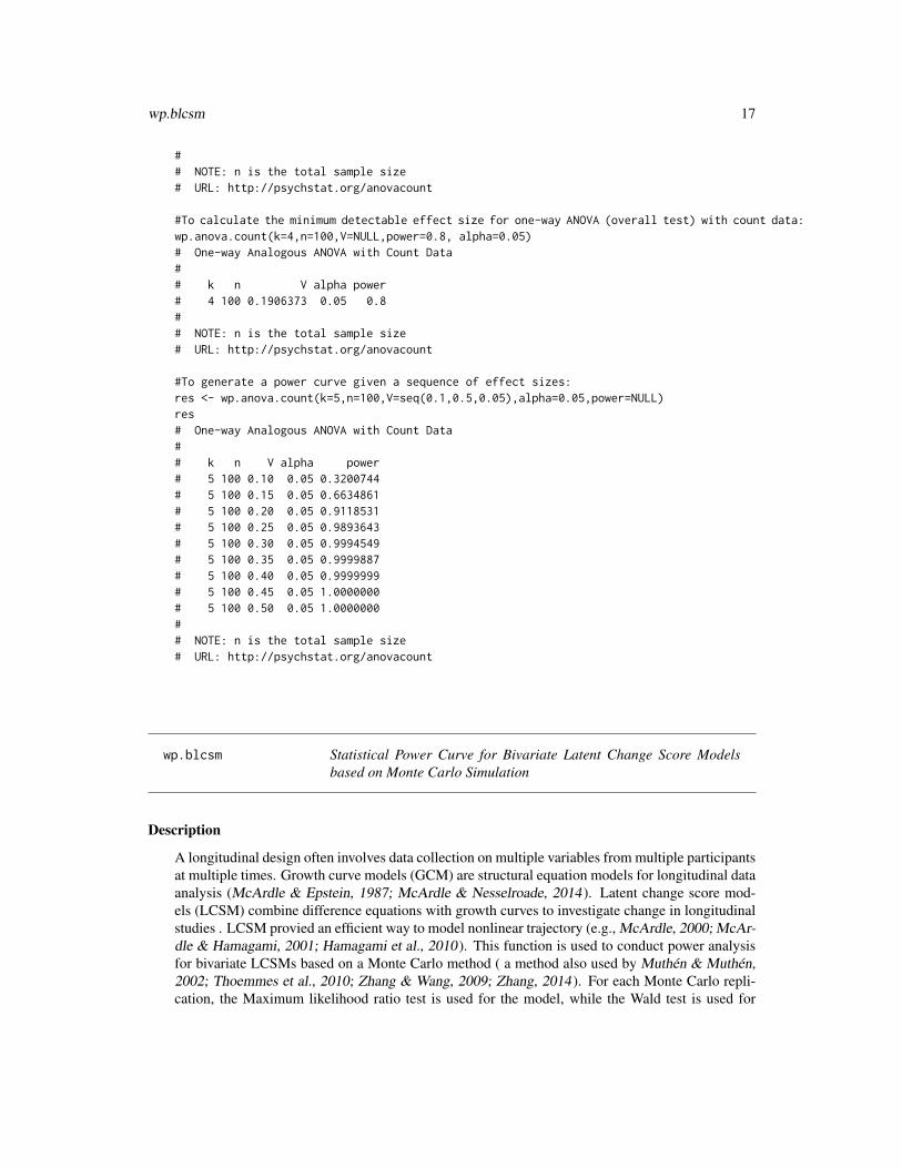
#To calculate the statistical power for one-way ANOVA (overall test) with count data:wp.anova.count(k=4,n=100,V=0.148,alpha=0.05)# One-way Analogous ANOVA with Count Data## k n V alpha power# 4 100 0.148 0.05 0.5597441## NOTE: n is the total sample size# URL: http://psychstat.org/anovacount

#To generate a power curve given sequence of sample sizes:res <- wp.anova.count(k=4,n=seq(100,200,10),V=0.148,alpha=0.05,power=NULL)res# One-way Analogous ANOVA with Count Data## k n V alpha power# 4 100 0.148 0.05 0.5597441# 4 110 0.148 0.05 0.6049618# 4 120 0.148 0.05 0.6470911# 4 130 0.148 0.05 0.6860351# 4 140 0.148 0.05 0.7217782# 4 150 0.148 0.05 0.7543699# 4 160 0.148 0.05 0.7839101# 4 170 0.148 0.05 0.8105368# 4 180 0.148 0.05 0.8344142# 4 190 0.148 0.05 0.8557241# 4 200 0.148 0.05 0.8746580## NOTE: n is the total sample size# URL: http://psychstat.org/anovacount


#To calculate the required sample size for one-way ANOVA (overall test) with count data:wp.anova.count(k=4,n=NULL,V=0.148,power=0.8, alpha=0.05)# One-way Analogous ANOVA with Count Data## k n V alpha power# 4 165.9143 0.148 0.05 0.8

wp.blcsm 17

## NOTE: n is the total sample size# URL: http://psychstat.org/anovacount

#To calculate the minimum detectable effect size for one-way ANOVA (overall test) with count data:wp.anova.count(k=4,n=100,V=NULL,power=0.8, alpha=0.05)# One-way Analogous ANOVA with Count Data## k n V alpha power# 4 100 0.1906373 0.05 0.8## NOTE: n is the total sample size# URL: http://psychstat.org/anovacount

#To generate a power curve given a sequence of effect sizes:res <- wp.anova.count(k=5,n=100,V=seq(0.1,0.5,0.05),alpha=0.05,power=NULL)res# One-way Analogous ANOVA with Count Data## k n V alpha power# 5 100 0.10 0.05 0.3200744# 5 100 0.15 0.05 0.6634861# 5 100 0.20 0.05 0.9118531# 5 100 0.25 0.05 0.9893643# 5 100 0.30 0.05 0.9994549# 5 100 0.35 0.05 0.9999887# 5 100 0.40 0.05 0.9999999# 5 100 0.45 0.05 1.0000000# 5 100 0.50 0.05 1.0000000## NOTE: n is the total sample size# URL: http://psychstat.org/anovacount

wp.blcsm Statistical Power Curve for Bivariate Latent Change Score Modelsbased on Monte Carlo Simulation

Description

A longitudinal design often involves data collection on multiple variables from multiple participantsat multiple times. Growth curve models (GCM) are structural equation models for longitudinal dataanalysis (McArdle & Epstein, 1987; McArdle & Nesselroade, 2014 ). Latent change score mod-els (LCSM) combine difference equations with growth curves to investigate change in longitudinalstudies . LCSM provied an efficient way to model nonlinear trajectory (e.g., McArdle, 2000; McAr-dle & Hamagami, 2001; Hamagami et al., 2010 ). This function is used to conduct power analysisfor bivariate LCSMs based on a Monte Carlo method ( a method also used by Muthén & Muthén,2002; Thoemmes et al., 2010; Zhang & Wang, 2009; Zhang, 2014 ). For each Monte Carlo repli-cation, the Maximum likelihood ratio test is used for the model, while the Wald test is used for

18 wp.blcsm

the parameter test. The method can obtain the power for testing each individual parameter of themodels such as the change rate and coupling parameters.

Usage

wp.blcsm(N = 100, T = 5, R = 1000, betay = 0, my0 = 0, mys = 0,varey = 1, vary0 = 1, varys = 1, vary0ys = 0, alpha = 0.05,betax = 0, mx0 = 0, mxs = 0, varex = 1, varx0 = 1, varxs = 1,varx0xs = 0, varx0y0 = 0, varx0ys = 0, vary0xs = 0, varxsys = 0,gammax = 0, gammay = 0, ...)

Arguments

N Sample size. It is 100 by default.

T Number of measurement occasions. It is 5 by default.

R Number of replications for the Monte Carlo simulation. It is 1000 by default.

betay Parameter in the model: The compound rate of change for variable y. Its defaultvalue is 0.

my0 Parameter in the model: Mean of the initial latent score for variable y. Its defaultvalue is 0.

mys Parameter in the model: Mean of the linear constant effect for variable y. Itsdefault value is 0.

varey Parameter in the model: Variance of the measurement error/uniqueness scorefor variable y. Its default value is 1.

vary0 Parameter in the model: Variance of the initial latent score for variable y. Itsdefault value is 1.

varys Parameter in the model: Variance of the linear constant effect for variable y. Itsdefault value is 0.

vary0ys Parameter in the model: Covariance of the initial latent score and the linearconstant effect for variable y. Its default value is 0.

alpha significance level chosed for the test. It equals 0.05 by default.

betax Parameter in the model: The compound rate of change for variable x. Its defaultvalue is 0.

mx0 Parameter in the model: Mean of the initial latent score for variable x. Its defaultvalue is 0.

mxs Parameter in the model: Mean of the linear constant effect for variable x. Itsdefault value is 0.

varex Parameter in the model: Variance of the measurement error/uniqueness scorefor variable x. Its default value is 1.

varx0 Parameter in the model: Variance of the initial latent score for variable x. Itsdefault value is 1.

varxs Parameter in the model: Variance of the linear constant effect for variable x. Itsdefault value is 0.

wp.blcsm 19

varx0xs Parameter in the model: Covariance of the initial latent score and the linearconstant effect for variable x. Its default value is 0.

varx0y0 Parameter in the model: Covariance of the initial latent scores for y and x. Itsdefault value is 0.

varx0ys Parameter in the model: Covariance of the initial latent score for x and the linearconstant effect for y. Its default value is 0.

vary0xs Parameter in the model: Covariance of the initial latent score for y and the linearconstant effect for x. Its default value is 0.

varxsys Parameter in the model: Covariance of the linear constant effects for y and x. Itsdefault value is 0.

gammax Coupling parameter in the model: The effect of variable x on the change scoreof variable y. Its default value is 0.

gammay Coupling parameter in the model: The effect of variable y on the change scoreof variable x. Its default value is 0.


Value

An object of the power analysis. The output of the R function includes 4 main pieces of informationfor each parameter in the model. The first is the Monte Carlo estimate (mc.est). It is calculated asthe mean of the R sets of parameter estimates from the simulated data. Note that the Monte Carloestimates should be close to the population parameter values used in the model. The second is theMonte Carlo standard deviation (mc.sd), which is calculated as the standard deviation of the R setsof parameter estimates. The third is the Monte Carlo standard error (mc.se), which is obtained asthe average of the R sets of standard error estimates of the parameter estimates. Lastly, mc.power isthe statistical power for each parameter.

References



Examples

## Not run:#To conduct power analysis for a bivariate LCSM with sample size equal to 100:wp.blcsm(N=100, T=5, R=1000, betay=0.08, my0=20, mys=1.5, varey=9,

vary0=3, varys=1, vary0ys=0, alpha=0.05, betax=0.2, mx0=20, mxs=5,varex=9, varx0=3, varxs=1, varx0xs=0, varx0y0=1, varx0ys=0,

vary0xs=0, varxsys=0, gammax=0, gammay=-.1)# pop.par mc.est mc.sd mc.se mc.power N T# betax 0.20 0.230 0.260 0.187 0.241 100 5# betay 0.08 0.164 0.572 0.435 0.081 100 5# gammax 0.00 -0.033 0.234 0.178 0.112 100 5# gammay -0.10 -0.175 0.641 0.458 0.075 100 5

20 wp.correlation

# mx0 20.00 20.004 0.336 0.326 1.000 100 5# mxs 5.00 5.933 7.848 5.615 0.167 100 5# my0 20.00 20.019 0.346 0.326 1.000 100 5# mys 1.50 0.451 6.933 5.321 0.156 100 5# varex 9.00 8.941 0.744 0.732 1.000 100 5# varey 9.00 8.939 0.749 0.720 1.000 100 5# varx0 3.00 3.029 1.243 1.222 0.739 100 5# varx0xs 0.00 -0.210 0.768 0.767 0.030 100 5# varx0y0 1.00 1.052 0.840 0.835 0.226 100 5# varx0ys 0.00 -0.012 0.668 0.601 0.017 100 5# varxs 0.60 2.343 6.805 2.687 0.090 100 5# varxsys 0.00 0.072 3.559 1.740 0.019 100 5# vary0 3.00 2.951 1.423 1.245 0.684 100 5# vary0xs 0.00 0.198 2.263 1.629 0.031 100 5# vary0ys 0.00 -0.371 1.970 1.511 0.106 100 5# varys 0.05 1.415 3.730 2.096 0.024 100 5

#To conduct power analysis for a bivariate LCSM with sample size equal to 500:wp.blcsm(N=500, T=5, R=1000, betay=0.08, my0=20, mys=1.5, varey=9,

vary0=3, varys=1, vary0ys=0, alpha=0.05, betax=0.2, mx0=20, mxs=5, varex=9, varx0=3, varxs=1, varx0xs=0, varx0y0=1,

varx0ys=0, vary0xs=0, varxsys=0, gammax=0, gammay=-.1)# pop.par mc.est mc.sd mc.se mc.power N T# betax 0.20 0.2009 0.031 0.031 1.000 500 5# betay 0.08 0.0830 0.070 0.068 0.199 500 5# gammax 0.00 -0.0014 0.030 0.029 0.057 500 5# gammay -0.10 -0.1022 0.072 0.073 0.271 500 5# mx0 20.00 19.9911 0.145 0.145 1.000 500 5# mxs 5.00 5.0308 0.939 0.942 1.000 500 5# my0 20.00 19.9999 0.143 0.146 1.000 500 5# mys 1.50 1.4684 0.889 0.885 0.420 500 5# varex 9.00 8.9836 0.340 0.328 1.000 500 5# varey 9.00 8.9961 0.341 0.328 1.000 500 5# varx0 3.00 3.0052 0.524 0.523 1.000 500 5# varx0xs 0.00 -0.0144 0.222 0.230 0.047 500 5# varx0y0 1.00 1.0064 0.360 0.360 0.808 500 5# varx0ys 0.00 -0.0012 0.199 0.201 0.051 500 5# varxs 1.00 1.0312 0.180 0.189 1.000 500 5# varxsys 0.00 0.0028 0.161 0.163 0.045 500 5# vary0 3.00 2.9777 0.519 0.547 1.000 500 5# vary0xs 0.00 0.0072 0.286 0.294 0.035 500 5# vary0ys 0.00 -0.0135 0.252 0.257 0.043 500 5# varys 1.00 1.0246 0.260 0.253 0.999 500 5

## End(Not run)

wp.correlation Statistical Power Analysis for Correlation

wp.correlation 21

Description

This function is for power analysis for correlation. Correlation measures whether and how a pairof variables are related. The Pearson Product Moment correlation coefficient (r) is adopted here.The power calculation for correlation is conducted based on Fisher’s z transformation of Pearsoncorrelation coefficent (Fisher, 1915, 1921).

Usage

wp.correlation(n = NULL, r = NULL, power = NULL, p = 0, rho0 = 0,alpha = 0.05, alternative = c("two.sided", "less", "greater"))

Arguments

n Sample size.

r Effect size or correlation. According to Cohen (1988), a correlation coefficientof 0.10, 0.30, and 0.50 are considered as an effect size of "small", "medium",and "large", respectively.


p Number of variables to partial out.

rho0 Null correlation coefficient.


alternative Direction of the alternative hypothesis ("two.sided" or "less" or "greater").The default is "two.sided".

Value


References


Fisher, R. A. (1915). Frequency distribution of the values of the correlation coefficient in samplesfrom an indefinitely large population. Biometrika, 10(4), 507-521.

Fisher, R. A. (1921). On the probable error of a coefficient of correlation deduced from a smallsample. Metron, 1, 3-32.


Examples

wp.correlation(n=50,r=0.3, alternative="two.sided")# Power for correlation## n r alpha power# 50 0.3 0.05 0.5728731#

22 wp.correlation

# URL: http://psychstat.org/correlation

#To calculate the power curve with a sequence of sample sizes:res <- wp.correlation(n=seq(50,100,10),r=0.3, alternative="two.sided")res# Power for correlation## n r alpha power# 50 0.3 0.05 0.5728731# 60 0.3 0.05 0.6541956# 70 0.3 0.05 0.7230482# 80 0.3 0.05 0.7803111# 90 0.3 0.05 0.8272250# 100 0.3 0.05 0.8651692## URL: http://psychstat.org/correlation


#To estimate the sample size with a given power:wp.correlation(n=NULL, r=0.3, power=0.8, alternative="two.sided")# Power for correlation## n r alpha power# 83.94932 0.3 0.05 0.8## URL: http://psychstat.org/correlation

#To estimate the minimum detectable effect size with a given power:wp.correlation(n=NULL,r=0.3, power=0.8, alternative="two.sided")# Power for correlation## n r alpha power# 83.94932 0.3 0.05 0.8## URL: http://psychstat.org/correlation##To calculate the power curve with a sequence of effect sizes:res <- wp.correlation(n=100,r=seq(0.05,0.8,0.05), alternative="two.sided")res# Power for correlation## n r alpha power# 100 0.05 0.05 0.07854715# 100 0.10 0.05 0.16839833# 100 0.15 0.05 0.32163978# 100 0.20 0.05 0.51870091# 100 0.25 0.05 0.71507374# 100 0.30 0.05 0.86516918# 100 0.35 0.05 0.95128316# 100 0.40 0.05 0.98724538# 100 0.45 0.05 0.99772995

wp.crt2arm 23

# 100 0.50 0.05 0.99974699# 100 0.55 0.05 0.99998418# 100 0.60 0.05 0.99999952# 100 0.65 0.05 0.99999999# 100 0.70 0.05 1.00000000# 100 0.75 0.05 1.00000000# 100 0.80 0.05 1.00000000## URL: http://psychstat.org/correlation

wp.crt2arm Statistical Power Analysis for Cluster Randomized Trials with 2 Arms

Description

Cluster randomized trials (CRT) are a type of multilevel design for the situation when the entirecluster is randomly assigned to either a treatment arm or a contral arm (Liu, 2013). The datafrom CRT can be analyzed in a two-level hierachical linear model, where the indicator variablefor treatment assignment is included in second level. If a study contains multiple treatments, thenmutiple indicators will be used. This function is for designs with 2 arms (i.e., a treatment and acontrol). Details leading to power calculation can be found in Raudenbush (1997) and Liu (2013).

Usage

wp.crt2arm(n = NULL, f = NULL, J = NULL, icc = NULL, power = NULL,alpha = 0.05, alternative = c("two.sided", "one.sided"))

Arguments

n Sample size. It is the number of individuals within each cluster.

f Effect size. It specifies either the main effect of treatment, or the mean differencebetween the treatment clusters and the control clusters.

J Number of clusters / sides. It tells how many clusters are considered in the studydesign. At least two clusters are required.

icc Intra-class correlation. ICC is calculated as the ratio of between-cluster varianceto the total variance. It quantifies the degree to which two randomly drawnobservations within a cluster are correlated.



alternative Type of the alternative hypothesis ("two.sided" or "one.sided"). The defaultis "two.sided". The option "one.sided" can be either "less" or "greater".

Value


24 wp.crt2arm

References

Liu, X. S. (2013). Statistical power analysis for the social and behavioral sciences: basic andadvanced techniques. Routledge.

Raudenbush, S. W. (1997). Statistical analysis and optimal design for cluster randomized trials.Psychological Methods, 2(2), 173.


Examples

#To calculate the statistical power given sample size and effect size:wp.crt2arm(f = 0.6, n = 20, J = 10, icc = 0.1, alpha = 0.05, power = NULL)# Cluster randomized trials with 2 arms## J n f icc power alpha# 10 20 0.6 0.1 0.5901684 0.05## NOTE: n is the number of subjects per cluster.# URL: http://psychstat.org/crt2arm

#To generate a power curve given a sequence of sample sizes:res <- wp.crt2arm(f = 0.6, n = seq(20,100,10), J = 10,

icc = 0.1, alpha = 0.05, power = NULL)res# Cluster randomized trials with 2 arms## J n f icc power alpha# 10 20 0.6 0.1 0.5901684 0.05# 10 30 0.6 0.1 0.6365313 0.05# 10 40 0.6 0.1 0.6620030 0.05# 10 50 0.6 0.1 0.6780525 0.05# 10 60 0.6 0.1 0.6890755 0.05# 10 70 0.6 0.1 0.6971076 0.05# 10 80 0.6 0.1 0.7032181 0.05# 10 90 0.6 0.1 0.7080217 0.05# 10 100 0.6 0.1 0.7118967 0.05## NOTE: n is the number of subjects per cluster.# URL: http://psychstat.org/crt2arm


#To calculate the required sample size given power and effect size:wp.crt2arm(f = 0.8, n = NULL, J = 10,

icc = 0.1, alpha = 0.05, power = 0.8)# Cluster randomized trials with 2 arms## J n f icc power alpha# 10 16.02558 0.8 0.1 0.8 0.05

wp.crt3arm 25

## NOTE: n is the number of subjects per cluster.# URL: http://psychstat.org/crt2arm

wp.crt3arm Statistical Power Analysis for Cluster Randomized Trials with 3 Arms

Description

Cluster randomized trials (CRT) are a type of multilevel design for the situation when the entirecluster is randomly assigned to either a treatment arm or a contral arm (Liu, 2013). The datafrom CRT can be analyzed in a two-level hierachical linear model, where the indicator variablefor treatment assignment is included in second level. If a study contains multiple treatments, thenmutiple indicators will be used. This function is for designs with 3 arms (i.e., two treatments and acontrol). Details leading to power calculation can be found in Raudenbush (1997) and Liu (2013).

Usage

wp.crt3arm(n = NULL, f = NULL, J = NULL, icc = NULL, power = NULL,alpha = 0.05, alternative = c("two.sided", "one.sided"),type = c("main", "treatment", "omnibus"))

Arguments


f Effect size. It specifies one of the three types of effects: the main effect oftreatment, the mean difference between the treatment clusters, and the controlclusters.

J Number of clusters / sides. It tells how many clusters are considered in the studydesign. At least two clusters are required.

icc Intra-class correlation. ICC is calculated as the ratio of between-cluster varianceto the total variance. It quantifies the degree to which two randomly drawnobservations within a cluster are correlated.




type Type of effect ("main" or "treatment" or "omnibus") with "main" as default.The type "main" tests the difference between the average tratment arms and thecontrol arm; Type "treatment" tests the differnce between the two treament arms;and Type "omnibus" tests whether the tree arms are all equivalent.

26 wp.crt3arm

Value


References




Examples

#To calculate the statistical power given sample size and effect size:wp.crt3arm(f = 0.5, n = 20, J = 10, icc = 0.1, alpha = 0.05, power = NULL)# Cluster randomized trials with 3 arms## J n f icc power alpha# 10 20 0.5 0.1 0.3940027 0.05## NOTE: n is the number of subjects per cluster.# URL: http://psychstat.org/crt3arm

#To generate a power curve given a sequence of sample sizes:res <- wp.crt3arm(f = 0.5, n = seq(20, 100, 10), J = 10,

icc = 0.1, alpha = 0.05, power = NULL)res# Cluster randomized trials with 3 arms## J n f icc power alpha# 10 20 0.5 0.1 0.3940027 0.05# 10 30 0.5 0.1 0.4304055 0.05# 10 40 0.5 0.1 0.4513376 0.05# 10 50 0.5 0.1 0.4649131 0.05# 10 60 0.5 0.1 0.4744248 0.05# 10 70 0.5 0.1 0.4814577 0.05# 10 80 0.5 0.1 0.4868682 0.05# 10 90 0.5 0.1 0.4911592 0.05# 10 100 0.5 0.1 0.4946454 0.05## NOTE: n is the number of subjects per cluster.# URL: http://psychstat.org/crt3arm


#To calculate the required sample size given power and effect size:wp.crt3arm(f = 0.8, n = NULL, J = 10, icc = 0.1, alpha = 0.05, power = 0.8)# Cluster randomized trials with 3 arms

wp.effect.CRT2arm 27

## J n f icc power alpha# 10 27.25145 0.8 0.1 0.8 0.05## NOTE: n is the number of subjects per cluster.# URL: http://psychstat.org/crt3arm

wp.effect.CRT2arm Effect size calculatator based on raw data for Cluster RandomizedTrials with 2 Arms

Description

This function is for effect size and ICC calculation for CRT with 2 arms based on empirical data.Cluster randomized trials (CRT) are a type of multilevel design for the situation when the entirecluster is randomly assigned to either a treatment arm or a contral arm (Liu, 2013). The datafrom CRT can be analyzed in a two-level hierachical linear model, where the indicator variablefor treatment assignment is included in second level. If a study contains multiple treatments, thenmutiple indicators will be used. This function is for designs with 3 arms (i.e., two treatments and acontrol). Details leading to power calculation can be found in Raudenbush (1997) and Liu (2013).The Effect size f specifies the main effect of treatment, the mean difference between the treatmentclusters and the control clusters. This function is used to calculate the effect size with a input dataset.

Usage

wp.effect.CRT2arm(file)

Arguments

file The input data set. The first column of the data is the ID variable, the secondcolumn represents cluster, the third column is the outcome variable, and thefourth column is the condition variable (0 for control, 1 for condition).

Value

A list including effect size f and ICC.

References



28 wp.effect.CRT3arm

Examples

#Empirical data set CRT2:CRT2#ID cluster score group#1 1 6 0#2 1 2 0#3 2 6 1#4 2 5 1#5 3 1 0#6 3 4 0#7 4 6 1#8 4 4 1

#To calculate the effect size and ICC based on empirical datawp.effect.CRT2arm (CRT2)# Effect size for CRT2arm## f ICC# 1.264911 -0.5## NOTE: f is the effect size.# URL: http://psychstat.org/crt2arm

wp.effect.CRT3arm Effect size calculatator based on raw data for Cluster RandomizedTrials with 3 Arms

Description

This function is for effect size and ICC calculation for Cluster randomized trials (CRT) with 3 armsbased on empirical data. CRT are a type of multilevel design for the situation when the entirecluster is randomly assigned to either a treatment arm or a contral arm (Liu, 2013). The datafrom CRT can be analyzed in a two-level hierachical linear model, where the indicator variablefor treatment assignment is included in second level. If a study contains multiple treatments, thenmutiple indicators will be used. This function is for designs with 3 arms (i.e., two treatments and acontrol). Details leading to power calculation can be found in Raudenbush (1997) and Liu (2013).The Effect size f specifies the main effect of treatment, the mean difference between the treatmentclusters and the control clusters. This function is used to calculate the effect size with a input dataset.

Usage

wp.effect.CRT3arm(file)

wp.effect.MRT2arm 29

Arguments

file The input data set. The first column of the data is the ID variable, the secondcolumn represents cluster, the third column is the outcome variable, and thefourth column is the condition variable (0 for control, 1 for treatment1, 2 fortreatment2).

Value

A list including effect size f1, f2, f3, and ICC.

References



Examples

#To calculate the effect sizes based on empirical datawp.effect.CRT3arm (CRT3)# Effect size for CRT3arm## f1 f2 f3 ICC# 0.6389258 -0.6189113 0.3931397 -0.019794## NOTE: f1 for treatment main effect;# f2 for difference between two treatments;# f3 for effect size of omnibus test.# URL: http://psychstat.org/crt3arm

wp.effect.MRT2arm Effect size calculatator based on raw data for Multisite RandomizedTrials with 2 Arms

Description

This function is for effect size calculation for Multisite randomized trials (MRT) with 2 arms basedon empirical data. MRTs are a type of multilevel design for the situation when the entire clusteris randomly assigned to either a treatment arm or a contral arm (Liu, 2013). The data from MRTcan be analyzed in a two-level hierachical linear model, where the indicator variable for treatmentassignment is included in first level. If a study contains multiple treatments, then mutiple indicatorswill be used. Three types of tests are considered in the function: (1) The "main" type tests treatmentmain effect; (2) The "site" type tests the variance of cluster/site means; and (3) The "variance" typetests variance of treatment effects. Details leading to power calculation can be found in Raudenbush(1997) and Liu (2013). This function is used to calculate the effect size with a input data set.

30 wp.effect.MRT3arm

Usage

wp.effect.MRT2arm(file)

Arguments

file The input data set. The first column of the data is the ID variable, the secondcolumn represents cluster, the third column is the outcome variable, and thefourth column is the condition variable (0 for control, 1 for condition).

Value

A list including effect size f.

References



Examples

#To calculate the effect size based on empirical datawp.effect.MRT2arm (MRT2)# Effect size for MRT2arm## f# -0.2986755## NOTE: f is the effect size.# URL: http://psychstat.org/mrt2arm

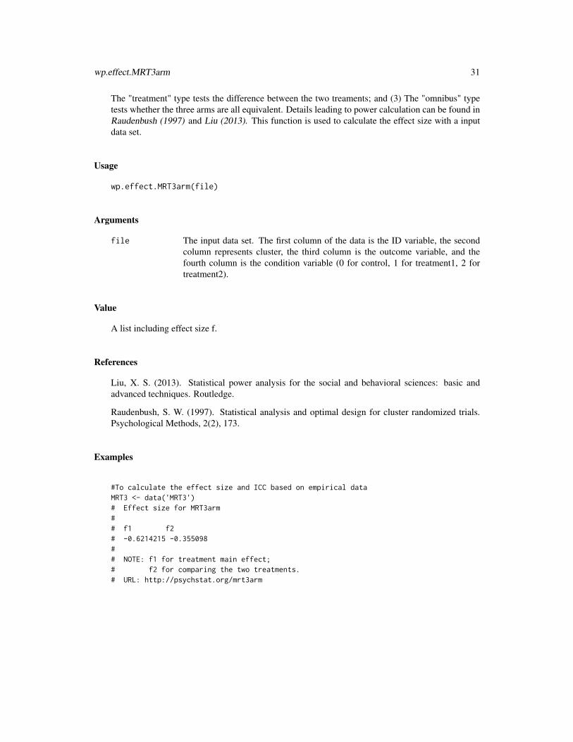
wp.effect.MRT3arm Effect size calculatator based on raw data for Multisite RandomizedTrials with 3 Arms

Description

This function is for effect size calculation for Multisite randomized trials (MRT) with 3 arms basedon empirical data. MRTs are a type of multilevel design for the situation when the entire clusteris randomly assigned to either a treatment arm or a contral arm (Liu, 2013). The data from MRTcan be analyzed in a two-level hierachical linear model, where the indicator variable for reatmentassignment is included in first level. If a study contains multiple treatments, then mutiple indicatorswill be used. This function is for designs with 3 arms (i.e., two treatments and a control). Threetypes of tests are considered in the function: (1) The "main" type tests treatment main effect; (2)

wp.effect.MRT3arm 31

The "treatment" type tests the difference between the two treaments; and (3) The "omnibus" typetests whether the three arms are all equivalent. Details leading to power calculation can be found inRaudenbush (1997) and Liu (2013). This function is used to calculate the effect size with a inputdata set.

Usage

wp.effect.MRT3arm(file)

Arguments

file The input data set. The first column of the data is the ID variable, the secondcolumn represents cluster, the third column is the outcome variable, and thefourth column is the condition variable (0 for control, 1 for treatment1, 2 fortreatment2).

Value

A list including effect size f.

References



Examples

#To calculate the effect size and ICC based on empirical dataMRT3 <- data('MRT3')# Effect size for MRT3arm## f1 f2# -0.6214215 -0.355098## NOTE: f1 for treatment main effect;# f2 for comparing the two treatments.# URL: http://psychstat.org/mrt3arm

32 wp.kanova

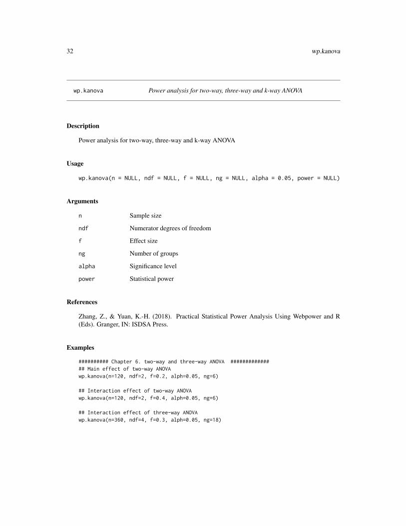
wp.kanova Power analysis for two-way, three-way and k-way ANOVA

Description

Power analysis for two-way, three-way and k-way ANOVA

Usage

wp.kanova(n = NULL, ndf = NULL, f = NULL, ng = NULL, alpha = 0.05, power = NULL)

Arguments

n Sample size

ndf Numerator degrees of freedom

f Effect size

ng Number of groups

alpha Significance level

power Statistical power

References


Examples

########## Chapter 6. two-way and three-way ANOVA ############### Main effect of two-way ANOVAwp.kanova(n=120, ndf=2, f=0.2, alph=0.05, ng=6)

## Interaction effect of two-way ANOVAwp.kanova(n=120, ndf=2, f=0.4, alph=0.05, ng=6)

## Interaction effect of three-way ANOVAwp.kanova(n=360, ndf=4, f=0.3, alph=0.05, ng=18)

wp.lcsm 33

wp.lcsm Statistical Power Curve for Univariate Latent Change Score Modelsbased on Monte Carlo Simulation

Description

A longitudinal design often involves data collection on multiple variables from multiple participantsat multiple times. Growth curve models (GCM) are structural equation models for longitudinal dataanalysis (McArdle & Epstein, 1987; McArdle & Nesselroade, 2014 ). Latent change score mod-els (LCSM) combine difference equations with growth curves to investigate change in longitudinalstudies . LCSM provied an efficient way to model nonlinear trajectory (e.g., McArdle, 2000; McAr-dle & Hamagami, 2001; Hamagami et al., 2010 ). This function is used to conduct power analysisfor univariate LCSMs based on a Monte Carlo method ( a method also used by Muthén & Muthén,2002; Thoemmes et al., 2010; Zhang & Wang, 2009; Zhang, 2014 ). For each Monte Carlo repli-cation, the Maximum likelihood ratio test is used for the model, while the Wald test is used forthe parameter test. The method can obtain the power for testing each individual parameter of themodels such as the change rate and coupling parameters.

Usage

wp.lcsm(N = 100, T = 5, R = 1000, betay = 0, my0 = 0, mys = 0,varey = 1, vary0 = 1, varys = 1, vary0ys = 0, alpha = 0.05, ...)

Arguments

N Sample size. It is 100 by default.

T Number of measurement occasions. It is 5 by default.

R Number of replications for the Monte Carlo simulation. It is 1000 by default.

betay Parameter in the model: The compound rate of change. Its default value is 0.

my0 Parameter in the model: Mean of the initial latent score. Its default value is 0.

mys Parameter in the model: Mean of the linear constant effect. Its default value is0.

varey Parameter in the model: Variance of the measurement error/uniqueness score.Its default value is 1.

vary0 Parameter in the model: Variance of the initial latent score. Its default value is1.

varys Parameter in the model: Variance of the linear constant effect. Its default valueis 0.

vary0ys Parameter in the model: Covariance of the initial latent score and the linearconstant effect. Its default value is 0.



34 wp.lcsm

Value

An object of the power analysis. The output of the R function includes 4 main pieces of informationfor each parameter in the model. The first is the Monte Carlo estimate (mc.est). It is calculated asthe mean of the R sets of parameter estimates from the simulated data. Note that the Monte Carloestimates should be close to the population parameter values used in the model. The second is theMonte Carlo standard deviation (mc.sd), which is calculated as the standard deviation of the R setsof parameter estimates. The third is the Monte Carlo standard error (mc.se), which is obtained asthe average of the R sets of standard error estimates of the parameter estimates. Lastly, mc.power isthe statistical power for each parameter.

References



Examples

## Not run:#Power analysis for a univariate LCSM#Power for each parameter given sample size, number of measurement occasions,# true effect (true values of parameters), and significance level:wp.lcsm(N = 100, T = 5, R = 1000, betay = 0.1, my0 = 20, mys = 1.5,

varey = 9, vary0 = 2.5, varys = .05, vary0ys = 0, alpha = 0.05)# pop.par mc.est mc.sd mc.se mc.power N T# betay 0.10 0.103 0.043 0.044 0.664 100 5# my0 20.00 19.999 0.324 0.319 1.000 100 5# mys 1.50 1.418 1.106 1.120 0.274 100 5# varey 9.00 8.961 0.724 0.732 1.000 100 5# vary0 2.50 2.463 1.151 1.139 0.583 100 5# vary0ys 0.00 -0.004 0.408 0.403 0.048 100 5# varys 0.05 0.053 0.173 0.175 0.050 100 5## #To calculate the Type I error rate and power for parameters

wp.lcsm(N = 100, T = 5, R = 1000, betay = 0, my0 = 0, mys = 0,varey = 1, vary0 = 1, varys = 1, vary0ys = 0,alpha = 0.05)

# pop.par mc.est mc.sd mc.se mc.power N T# betay 0 0.001 0.056 0.056 0.046 100 5# my0 0 0.001 0.129 0.126 0.056 100 5# mys 0 0.002 0.105 0.105 0.044 100 5# varey 1 0.994 0.083 0.081 1.000 100 5# vary0 1 0.990 0.236 0.230 1.000 100 5# vary0ys 0 -0.005 0.136 0.136 0.044 100 5# varys 1 1.006 0.227 0.227 1.000 100 5

# To generate a power curve for different sample sizes for a univariate LCSMres <- wp.lcsm(N = seq(100, 200, 10), T = 5, R = 1000, betay = 0.1,

my0 = 20, mys = 1.5, varey = 9, vary0 = 2.5,varys = .05, vary0ys = 0, alpha = 0.05)

wp.logistic 35

#plot(res, parameter='betay')#plot(res, parameter='mys')

# To generate a power curve for different numbers of occasions for a univariate LCSMres <- wp.lcsm(N = 100, T = 4:10, R = 1000, betay = 0.1, my0 = 20, mys = 1.5,

varey = 9, vary0 = 2.5, varys = .05, vary0ys = 0, alpha = 0.05)#plot(res, parameter='betay')#plot(res, parameter='mys')

## End(Not run)

wp.logistic Statistical Power Analysis for Logistic Regression

Description

This function is for Logistic regression models. Logistic regression is a type of generalized linearmodels where the outcome variable follows Bernoulli distribution. Here, Maximum likelihoodmethods is used to estimate the model parameters. The estimated regression coefficent is assumedto follow a normal distribution. A Wald test is use to test the mean difference between the estimatedparameter and the null parameter (tipically the null hypothesis assumes it equals 0). The procedureintroduced by Demidenko (2007) is adopted here for computing the statistical power.

Usage

wp.logistic(n = NULL, p0 = NULL, p1 = NULL, alpha = 0.05,power = NULL, alternative = c("two.sided", "less", "greater"),family = c("Bernoulli", "exponential", "lognormal", "normal", "Poisson","uniform"), parameter = NULL)

Arguments

n Sample size.p0 Prob(Y=1|X=0 ): the probobility of observieng 1 for the outcome variable Y

when the predictor X equals 0.p1 Prob(Y=1|X=1 ): the probobility of observieng 1 for the outcome variable Y

when the predictor X equals 1.alpha significance level chosed for the test. It equals 0.05 by default.power Statistical power.alternative Direction of the alternative hypothesis ("two.sided" or "less" or "greater").

The default is "two.sided".family Distribution of the predictor ("Bernoulli","exponential", "lognormal", "normal",

"Poisson", "uniform"). The default is "Bernoulli".parameter Corresponding parameter for the predictor’s distribution. The default is 0.5 for

"Bernoulli", 1 for "exponential", (0,1) for "lognormal" or "normal", 1 for "Pois-son", and (0,1) for "uniform".

36 wp.logistic

Value


References

Demidenko, E. (2007). Sample size determination for logistic regression revisited. Statistics inmedicine, 26(18), 3385-3397.


Examples

#To calculate the statistical power given sample size and effect size:wp.logistic(n = 200, p0 = 0.15, p1 = 0.1, alpha = 0.05,

power = NULL, family = "normal", parameter = c(0,1))# Power for logistic regression## p0 p1 beta0 beta1 n alpha power# 0.15 0.1 -1.734601 -0.4626235 200 0.05 0.6299315## URL: http://psychstat.org/logistic

#To generate a power curve given a sequence of sample sizes:res <- wp.logistic(n = seq(100,500,50), p0 = 0.15, p1 = 0.1, alpha = 0.05,

power = NULL, family = "normal", parameter = c(0,1))res# Power for logistic regression## p0 p1 beta0 beta1 n alpha power# 0.15 0.1 -1.734601 -0.4626235 100 0.05 0.3672683# 0.15 0.1 -1.734601 -0.4626235 150 0.05 0.5098635# 0.15 0.1 -1.734601 -0.4626235 200 0.05 0.6299315# 0.15 0.1 -1.734601 -0.4626235 250 0.05 0.7264597# 0.15 0.1 -1.734601 -0.4626235 300 0.05 0.8014116# 0.15 0.1 -1.734601 -0.4626235 350 0.05 0.8580388# 0.15 0.1 -1.734601 -0.4626235 400 0.05 0.8998785# 0.15 0.1 -1.734601 -0.4626235 450 0.05 0.9302222# 0.15 0.1 -1.734601 -0.4626235 500 0.05 0.9518824## URL: http://psychstat.org/logistic


#To calculate the required sample size given power and effect size:wp.logistic(n = NULL, p0 = 0.15, p1 = 0.1, alpha = 0.05,

power = 0.8, family = "normal", parameter = c(0,1))# Power for logistic regression## p0 p1 beta0 beta1 n alpha power

wp.mc.sem.basic 37

# 0.15 0.1 -1.734601 -0.4626235 298.9207 0.05 0.8## URL: http://psychstat.org/logistic

wp.mc.sem.basic Statistical Power Analysis for Structural Equation Modeling / Media-tion based on Monte Carlo Simulation

Description

Structural equation modeling (SEM) is a multivariate technique used to analyze relationships amongobserved and latent variables. It can be viewed as a combination of factor analysis and multivariateregression analysis. A mediation model can be viewed as a SEM model. Funtions wp.sem.chisqand wp.sem.rmsea provide anlytical solutions of power analysis for SEM. Function wp.mediationprovides anlytical solutions of power analysis for a simple mediatoin model. This function providesa solution based on Monte Carlo simulation (see Zhang, 2014 ). If the model is a mediation, Sobeltest is used for the mediation / indirect effects. The solution is extended from the general frameworkfor power analysis for complex mediation models using Monte Carlo simulation in Mplus (Muthén& Muthén, 2011) proposed by Thoemmes et al. (2010). We extended the framework in two ways.First, the method allows the specification of nonnormal data in the Monte Carlo simulation and canthereby reflect more closely practical data collection. Second, the function wp.mc.sem.basic of afree, open-source R package, WebPower, is developed to ease power anlysis for mediation modelsusing the proposed method.

Usage

wp.mc.sem.basic(model, indirect = NULL, nobs = 100, nrep = 1000,alpha = 0.95, skewness = NULL, kurtosis = NULL, ovnames = NULL,se = "default", estimator = "default", parallel = "no",ncore = Sys.getenv("NUMBER_OF_PROCESSORS"), cl = NULL, ...)

Arguments

model Model specified using lavaan syntax. More about model specification can befound in Rosseel (2012).

indirect Indirect effect difined using lavaan syntax.

nobs Sample size.

nrep Number of replications for the Monte Carlo simulation.


skewness A sequence of skewnesses of the observed variables.

kurtosis A sequence of kurtosises of the observed variables.

ovnames Names of the observed variables in the model.

38 wp.mc.sem.basic

se The method for calculatating the standard errors. Its default method "default"is regular standard errors. More about methods specification standard errorscalculatationcan be found in Rosseel (2012).

estimator Estimator. It is Maxmum likelihood estimator by default. More about estimatorspecification can be found in Rosseel (2012).

parallel Parallel computing ("no" or "parallel" or "snow"). It is "no" by default,which means it will not use parallel computing. The option "parallel" is to usemultiple cores in a computer for parallel computing. It is used with the numberof cores (ncore). The option "snow" is to use clusters for parallel computing. Itis used with the number of clusters (cl ).

ncore Number of processors used for parallel computing. By default, ncore = Sys.getenv(’NUMBER_OF_PROCESSORS’).

cl Number of clusters. It is NULL by default. When it is NULL, the program willdetect the number of clusters automatically.


Value

An object of the power analysis. The power for all parameters in the model as well as the indirecteffects if specified.

References

MacCallum, R. C., Browne, M. W., & Sugawara, H. M. (1996). Power analysis and determinationof sample size for covariance structure modeling. Psychological methods, 1(2), 130.

Rosseel, Y. (2012). Lavaan: An R package for structural equation modeling and more. Version0.5–12 (BETA). Ghent, Belgium: Ghent University.

Satorra, A., & Saris, W. E. (1985). Power of the likelihood ratio test in covariance structure analysis.Psychometrika, 50(1), 83-90.

Thoemmes, F., MacKinnon, D. P., & Reiser, M. R. (2010). Power analysis for complex mediationaldesigns using Monte Carlo methods. Structural Equation Modeling, 17(3), 510-534.

Zhang, Z. (2014). Monte Carlo based statistical power analysis for mediation models: Methods andsoftware. Behavior research methods, 46(4), 1184-1198.


Examples

## Not run:#To calculate power for mediation based on Monte Carlo simulation when Sobel test is used:#To specify the modeldemo ="y ~ cp*x + start(0)*x + b*m + start(0.39)* mm ~ a*x + start(0.39)*xx ~~ start(1)*xm ~~ start(1)*my ~~ start(1)*y"

wp.mc.sem.basic 39

#To specify the indirect effectsmediation = "ab := a*babc:= a*b + cp"#To calculate power for mediation using regular standard errorssobel.regular = wp.mc.sem.basic(model=demo, indirect=mediation, nobs=100, nrep=1000,

parallel="snow", skewness=c(0, 0, 1.3), kurtosis=c(0,0,10), ovnames=c("x","m","y"))

#To calculate power for mediation using robust standard errorssobel.robust = wp.mc.sem.basic(model=demo, indirect=mediation, nobs=100, nrep=1000,

parallel="snow", skewness=c(0, 0, 1.3), kurtosis=c(0,0,10), ovnames=c("x","m","y"), se="robust")

#To print the power for mediation based on Sobel test using regular standard errors:summary(sobel.regular)# Basic information:## Esimation method ML# Standard error standard# Number of requested replications 1000# Number of successful replications 1000## True Estimate MSE SD Power Coverage# Regressions:# y ~# x (cp) 0.000 0.003 0.106 0.107 0.045 0.955# m (b) 0.390 0.387 0.099 0.113 0.965 0.919# m ~# x (a) 0.390 0.389 0.100 0.101 0.976 0.953# Variances:# x 1.000 0.995 0.141 0.139 1.000 0.936# m 1.000 0.981 0.139 0.137 1.000 0.923# y 1.000 0.968 0.137 0.330 1.000 0.560## Indirect/Mediation effects:# ab 0.152 0.150 0.056 0.060 0.886 0.928# abc 0.152 0.153 0.106 0.109 0.305 0.948

#To print the power analysis results for mediation based on Sobel test using robust standard errors:summary(sobel.robust)# Basic information:## Esimation method ML# Standard error robust.sem# Number of requested replications 1000# Number of successful replications 1000## True Estimate MSE SD Power Coverage# Regressions:# y ~# x (cp) 0.000 -0.003 0.106 0.113 0.055 0.945# m (b) 0.390 0.398 0.111 0.119 0.972 0.927# m ~

40 wp.mc.sem.boot

# x (a) 0.390 0.389 0.099 0.101 0.974 0.939## Intercepts:# y 0.000 0.000 0.100 0.104 0.058 0.942# m 0.000 0.000 0.100 0.105 0.054 0.946# x 0.000 -0.004 0.100 0.104 0.066 0.934## Variances:# x 1.000 0.991 0.138 0.140 1.000 0.930# m 1.000 0.976 0.135 0.135 1.000 0.915# y 1.000 1.002 0.281 0.365 0.981 0.805## Indirect/Mediation effects:# ab 0.152 0.156 0.060 0.064 0.870 0.900# abc 0.152 0.153 0.108 0.117 0.303 0.936

## End(Not run)

wp.mc.sem.boot Statistical Power Analysis for Structural Equation Modeling / Media-tion based on Monte Carlo Simulation: bootstrap method

Description

Structural equation modeling (SEM) is a multivariate technique used to analyze relationships amongobserved and latent variables. It can be viewed as a combination of factor analysis and multivariateregression analysis. A mediation model can be viewed as a SEM model. Funtions wp.sem.chisqand wp.sem.rmsea provide anlytical solutions of power analysis for SEM. Function wp.mediationprovides anlytical solutions of power analysis for a simple mediatoin model. This function providesa solution based on Monte Carlo simulation (see Zhang, 2014 ) and a bootstrap method for testingthe indirect /mediation effects. The solution is extended from the general framework for poweranalysis for complex mediation models using Monte Carlo simulation in Mplus (Muthén & Muthén,2011) proposed by Thoemmes et al. (2010). We extended the framework in three ways. First, weproposes a general method to conduct power analysis for mediation models based on the bootstrapmethod. The method is still based on Monte Carlo simulation but uses the bootstrap method totest mediation effects. Second, the method allows the specification of nonnormal data in the MonteCarlo simulation and can thereby reflect more closely practical data collection. Third, the functionwp.mc.sem.boot of a free, open-source R package, WebPower, is developed to ease power anlysisfor mediation models using the proposed method.

Usage

wp.mc.sem.boot(model, indirect = NULL, nobs = 100, nrep = 1000,nboot = 1000, alpha = 0.95, skewness = NULL, kurtosis = NULL,ovnames = NULL, se = "default", estimator = "default",parallel = "no", ncore = Sys.getenv("NUMBER_OF_PROCESSORS"), cl = NULL,...)

wp.mc.sem.boot 41

Arguments



nobs Sample size. It is 100 by default.

nrep Number of replications for the Monte Carlo simulation. It is 1000 by default.

nboot Number of replications for the bootstrap to test the specified parameter (e.g.,mediation). It is 1000 by default.


skewness A sequence of skewnesses of the observed variables. It is not required.

kurtosis A sequence of kurtosises of the observed variables. It is not required.

ovnames Names of the observed variables in the model. It is not required.







Value


References



Zhang, Z. (2014). Monte Carlo based statistical power analysis for mediation models: Methods andsoftware. Behavior research methods, 46(4), 1184-1198.


42 wp.mc.sem.boot

Examples

## Not run:#To specify the modeldemo ="y ~ cp*x + start(0)*x + b*m + start(0.39)* mm ~ a*x + start(0.39)*xx ~~ start(1)*xm ~~ start(1)*my ~~ start(1)*y"#To specify the indirect effectsmediation = "ab := a*babc:= a*b + cp"#Power for mediation based on MC method when bootstrap method is used to test the effects:mediation.boot = wp.mc.sem.boot(model=demo, indirect=mediation, nobs=100,

nrep=1000, nboot=2000, parallel="parallel",skewness=c(0, 0, 1.3), kurtosis=c(0,0,10), ovnames=c("x","m","y"))

#To print the power analysis resultssummary(mediation.boot)

#Example: Power for Simple Mediation Analysisex1model <- "math ~ c*ME + start(0)*ME + b*HE + start(0.39)*HEHE ~ a*ME + start(0.39)*ME"

indirect <- "ab:=a*b"

boot.normal <- wp.mc.sem.boot(ex1model,indirect, 50, nrep=2000,nboot=2000, parallel='parallel')

summmary(boot.normal)

boot.non.normal <- wp.mc.sem.boot(ex1model,indirect, 100, nrep=2000,nboot=2000, parallel='parallel', skewness=c(-0.3, -0.7, 1.3),

kurtosis=c(1.5, 0, 5), ovnames=c('ME','HE','math'))summmary(boot.non.normal)

#Example: Multiple Group Mediation Analysis (Moderated Mediation)ex3model <- "y ~ start(c(0.283, 0.283))*x + c(c1,c2)*x + start(c(0.36, 0.14))*m + c(b1,b2)*mm ~ start(c(0.721, 0.721))*x + c(a1,a2)*xm =~ c(1,1)*m1 + start(c(0.8, 0.8))*m2 + start(c(0.8, 0.8))*m3x ~~ start(c(0.25, 0.25))*xy ~~ start(c(0.81, 0.95))*ym ~~ start(c(0.87, 0.87))*mm1 ~~ start(c(0.36, 0.36))*m1m2 ~~ start(c(0.36, 0.36))*m2m3 ~~ start(c(0.36, 0.36))*m3"

wp.mc.sem.power.curve 43

# med1 and med2 are the mediation effect for group1 and group2, respectively.indirect <- "med1 := a1*b1med2 := a2*b2diffmed := a1*b1 - a2*b2"

bootstrap <- wp.mc.sem.boot(ex3model, indirect, nobs=c(400,200),nrep=2000, nboot=1000, prallel='parallel')

summary(bootstrap)

#Example: A Longitudinal Mediation Modelex4model <- "x2 ~ start(.9)*x1 + x*x1x3 ~ start(.9)*x2 + x*x2m2 ~ start(.3)*x1 + a*x1 + start(.3)*m1 + m*m1m3 ~ start(.3)*x2 + a*x2 + start(.3)*m2 + m*m2y2 ~ start(.3)*m1 + b*m1 + start(.7)*y1 + y*y1y3 ~ start(.3)*m2 + b*m2 + start(.7)*y2 + y*y2 + start(0)*x1 + c*x1x1 ~~ start(.37)*m1x1 ~~ start(.27)*y1y1 ~~ start(.2278)*m1x2 ~~ start(.19)*x2x3 ~~ start(.19)*x3m2 ~~ start(.7534)*m2m3 ~~ start(.7534)*m3y2 ~~ start(.3243)*y2y3 ~~ start(.3243)*y3"

indirect <- "ab := a*b"

bootstrap <- wp.mc.sem.boot(ex4model, indirect, nobs=50, nrep=1000,nboot=1000, parallel='parallel', ncore=8)

summary(bootstrap)

## End(Not run)

wp.mc.sem.power.curve Statistical Power Curve for Structural Equation Modeling / Mediationbased on Monte Carlo Simulation

Description

A power curve is useful to graphically display how power changes with sample size (e.g., Zhang& Wang). This function is to generate a power curve for SEM based on Monte Carlo simulation,either using Sobel test or bootstrap method to test the indirect / mediation effects if applicable.

44 wp.mc.sem.power.curve

Usage

wp.mc.sem.power.curve(model, indirect = NULL, nobs = 100, type = "basic",nrep = 1000, nboot = 1000, alpha = 0.95, skewness = NULL,kurtosis = NULL, ovnames = NULL, se = "default",estimator = "default", parallel = "no",ncore = Sys.getenv("NUMBER_OF_PROCESSORS"), cl = NULL, ...)

Arguments



nobs Sample size. It is 100 by default.

type The method used to test the indirect effects ('basic' or 'boot'). By defaulttype=’basic’. The type ’basic’ is to use Sobel test (see also wp.mc.sem.basic),while ’boot’ is to use bootstrap method (see also wp.mc.sem.boot).

nrep Number of replications for the Monte Carlo simulation. It is 1000 by default.

nboot Number of replications for the bootstrap to test the specified parameter (e.g.,mediation). It is 1000 by default.


skewness A sequence of skewnesses of the observed variables. It is not required.

kurtosis A sequence of kurtosises of the observed variables. It is not required.

ovnames Names of the observed variables in the model. It is not required.







Value


wp.mc.t 45

References




Examples

## Not run:#To specify the modelex2model ="ept ~ start(0.4)*hvltt + b*hvltt + start(0)*age + start(0)*edu + start(2)*Rhvltt ~ start(-0.35)*age + a*age +c*edu + start(0.5)*eduR ~ start(-0.06)*age + start(0.2)*eduR =~ 1*ws + start(0.8)*ls + start(0.5)*ltage ~~ start(30)*ageedu ~~ start(8)*eduage ~~ start(-2.8)*eduhvltt ~~ start(23)*hvlttR ~~ start(14)*Rws ~~ start(3)*wsls ~~ start(3)*lslt ~~ start(3)*ltept ~~ start(3)*ept"#To specify the indirect effectsindirect = "ind1 := a*b + c*b"nobs <- seq(100, 2000, by =200)#To calculate power curve:power.curve = wp.mc.sem.power.curve(model=ex2model, indirect=indirect,

nobs=nobs, type='boot', parallel="muticore")

## End(Not run)

wp.mc.t Power analysis for t-test based on Monte Carlo simulation

Description

Power analysis for t-test based on Monte Carlo simulation

46 wp.mc.t

Usage

wp.mc.t(n = NULL, R0 = 1e+05, R1 = 1000, mu0 = 0, mu1 = 0,sd = 1, skewness = 0, kurtosis = 3, alpha = 0.05,type = c("two.sample", "one.sample", "paired"),alternative = c("two.sided", "less", "greater"))

Arguments

n Sample size

R0 Number of replications under the null

R1 Number of replications

mu0 Population mean under the null

mu1 Population mean under the alternative

sd Standard deviation

skewness Skewness

kurtosis kurtosis

alpha Significance level

type Type of anlaysis

alternative alternative hypothesis

References


Examples

########## Chapter 16. Monte Carlo t-test #############wp.mc.t(n=20 , mu0=0, mu1=0.5, sd=1, skewness=0,kurtosis=3, type = c("one.sample"), alternative = c("two.sided"))

wp.mc.t(n=40 , mu0=0, mu1=0.3, sd=1, skewness=1,kurtosis=6, type = c("paired"), alternative = c("greater"))

wp.mc.t(n=c(15, 15), mu1=c(0.2, 0.5), sd=c(0.2, 0.5),skewness=c(1, 2), kurtosis=c(4, 6), type = c("two.sample"), alternative = c("less"))

wp.mediation 47

wp.mediation Statistical Power Analysis for Simple Mediation

Description

This function is for mediation models. Mediation models can be used to investigate the underlyingmechanisms related to why an input variable x influences an output variable y (e.g., Hayes, 2013;MacKinnon, 2008 ). The mediation effect is calculated as a*b, where a is the path coefficent fromthe predictor x to the mediator m, and b is the path coefficent from the mediator m to the out-come variable y. Sobel test statistic (Sobel, 1982) is used to test whether the mediation effect issignificantly different from zero.

Usage

wp.mediation(n = NULL, power = NULL, a = 0.5, b = 0.5, varx = 1,vary = 1, varm = 1, alpha = 0.05)

Arguments

n Sample size.


a Coefficient from x to m. The default value is 0.5.

b Coefficient from m to y. The default value is 0.5.

varx Variance of x. The default value is 1.

vary Variance of y. The default value is 1.

varm Variance of m. The default value is 1.


Value


References

Hayes, A. F. (2013). Introduction to mediation, moderation, and conditional process analysis: Aregression-based approach. Guilford Press.

MacKinnon, D. P. (2008). Introduction to statistical mediation analysis. Routledge.

Sobel, M. E. (1982). Asymptotic confidence intervals for indirect effects in structural equationmodels. Sociological methodology, 13, 290-312.


48 wp.mediation

Examples

#To calculate the statistical power given sample size and effect size:wp.mediation(n = 100, power = NULL, a = 0.5, b = 0.5,

varx = 1, vary = 1, varm = 1, alpha = 0.05)# Power for simple mediation## n power a b varx varm vary alpha# 100 0.9337271 0.5 0.5 1 1 1 0.05## URL: http://psychstat.org/mediation

#To generate a power curve given a sequence of sample sizes:res <- wp.mediation(n = seq(50,100,5), power = NULL, a = 0.5, b = 0.5,

varx = 1, vary = 1, varm = 1, alpha = 0.05)res# Power for simple mediation## n power a b varx varm vary alpha# 50 0.6877704 0.5 0.5 1 1 1 0.05# 55 0.7287681 0.5 0.5 1 1 1 0.05# 60 0.7652593 0.5 0.5 1 1 1 0.05# 65 0.7975459 0.5 0.5 1 1 1 0.05# 70 0.8259584 0.5 0.5 1 1 1 0.05# 75 0.8508388 0.5 0.5 1 1 1 0.05# 80 0.8725282 0.5 0.5 1 1 1 0.05# 85 0.8913577 0.5 0.5 1 1 1 0.05# 90 0.9076417 0.5 0.5 1 1 1 0.05# 95 0.9216744 0.5 0.5 1 1 1 0.05# 100 0.9337271 0.5 0.5 1 1 1 0.05## URL: http://psychstat.org/mediation


#To calculate the required sample size given power and effect size:wp.mediation(n = NULL, power = 0.9, a = 0.5, b = 0.5,

varx = 1, vary = 1, varm = 1, alpha = 0.05)# Power for simple mediation## n power a b varx varm vary alpha# 87.56182 0.9 0.5 0.5 1 1 1 0.05## URL: http://psychstat.org/mediation

#To calculate the minimum detectable effect size of one coefficent given power and sample size:wp.mediation(n = 100, power = 0.9, a = NULL, b = 0.5,

varx = 1, vary = 1, varm = 1, alpha = 0.05)# Power for simple mediation## n power a b varx varm vary alpha

wp.mmrm 49

# 100 0.9 0.7335197 0.5 1 1 1 0.05## URL: http://psychstat.org/mediation

wp.mmrm Power analysis for longitudinal data analysis

Description

The two functions are adapted from the R package longpower by Michael C. Donohue. More willbe added later.

Usage

wp.mmrm(N = NULL, Ra = NULL, ra = NULL, sigmaa = NULL,Rb = NULL, rb = NULL, sigmab = NULL, lambda = 1,delta = NULL, alpha = 0.05, power = NULL,alternative = c("two.sided", "one.sided"))wp.mmrm.ar1(N = NULL, rho = NULL, ra = NULL, sigmaa = NULL,rb = NULL, sigmab = NULL, lambda = 1, times = 1:length(ra),delta = NULL, alpha = 0.05, power = NULL,alternative = c("two.sided", "one.sided"))

Arguments

N NRa Rara rasigmaa sigmaaRb Rbrb rbsigmab sigmablambda lambdadelta deltaalpha Significance levelpower Statistical poweralternative alternative hypothesisrho rhotimes times

References

Lu, K., Luo, X., Chen, P.-Y. (2008) Sample size estimation for repeated measures analysis in ran-domized clinical trials with missing data. International Journal of Biostatistics, 4, (1)

50 wp.mrt2arm

wp.mrt2arm Statistical Power Analysis for Multisite Randomized Trials with 2Arms

Description

Multisite randomized trials (MRT) are a type of multilevel design for the situation when the entirecluster is randomly assigned to either a treatment arm or a contral arm (Liu, 2013). The datafrom MRT can be analyzed in a two-level hierachical linear model, where the indicator variable fortreatment assignment is included in first level. If a study contains multiple treatments, then mutipleindicators will be used. This function is for designs with 2 arms (i.e., a treatment and a control).Three types of tests are considered in the function: (1) The "main" type tests treatment main effect;(2) The "site" type tests the variance of cluster/site means; and (3) The "variance" type tests varianceof treatment effects. Details leading to power calculation can be found in Raudenbush (1997) andLiu (2013).

Usage

wp.mrt2arm(n = NULL, f = NULL, J = NULL, tau00 = NULL, tau11 = NULL,sg2 = NULL, power = NULL, alpha = 0.05, alternative = c("two.sided","one.sided"), type = c("main", "site", "variance"))

Arguments


f Effect size. It specifies the main effect of treatment, the mean difference betweenthe treatment clusters/sites and the control clusters/sites. Effect size must bepositive.

J Number of clusters / sites. It tells how many clusters are considered in the studydesign. At least two clusters are required.

tau00 Variance of cluster/site means. It is one of the residual variances in the secondlevel. Its value must be positive.

tau11 Variance of treatment effects across sites. It is one of the residual variances inthe second level. Its value must be positive.

sg2 Level-one error Variance. The residual variance in the first level.




type Type of effect ("main" or "site" or "variance") with "main" as default. Thetype "main" tests treatment main effect, no tau00 needed; Type "site" tests thevariance of cluster/site means, no tau11 or f needed; and Type "variance" testsvariance of treatment effects, no tau00 or f needed.

wp.mrt2arm 51

Value


References




Examples

#To calculate the statistical power given sample size and effect size:#For main effectwp.mrt2arm(n = 45, f = 0.5, J = 20, tau11 = 0.5,

sg2 = 1.25, alpha = 0.05, power = NULL)# Power analysis for Multileve model Multisite randomized trials with 2 arms## J n f tau11 sg2 power alpha# 20 45 0.5 0.5 1.25 0.8583253 0.05## NOTE: n is the number of subjects per cluster# URL: http://psychstat.org/mrt2arm

#For variance of treament effectwp.mrt2arm(n = 45, f = 0.5, J = 20, tau11 = 0.5,

sg2 = 1.25, alpha = 0.05, power = NULL, type = "variance")# Power analysis for Multileve model Multisite randomized trials with 2 arms## J n f tau11 sg2 power alpha# 20 45 0.5 0.5 1.25 0.9987823 0.05## NOTE: n is the number of subjects per cluster# URL: http://psychstat.org/mrt2arm

#For testing site variablityres<- wp.mrt2arm(n = 45, f = 0.5, J = 20, tau11 = 0.5,

sg2 = 1.25, alpha = 0.05, power = NULL, type = "site")# Power analysis for Multileve model Multisite randomized trials with 2 arms## J n f tau11 sg2 alpha# 20 45 0.5 0.5 1.25 0.05## NOTE: n is the number of subjects per cluster# URL: http://psychstat.org/mrt2arm

#To generate a power curve given a sequence of sample sizes:wp.mrt2arm(n = seq(10,50,5), f = 0.5, J = 20, tau11 = 0.5,

52 wp.mrt3arm

sg2 = 1.25, alpha = 0.05, power = NULL)# Power analysis for Multileve model Multisite randomized trials with 2 arms## J n f tau11 sg2 power alpha# 20 10 0.5 0.5 1.25 0.6599499 0.05# 20 15 0.5 0.5 1.25 0.7383281 0.05# 20 20 0.5 0.5 1.25 0.7818294 0.05# 20 25 0.5 0.5 1.25 0.8090084 0.05# 20 30 0.5 0.5 1.25 0.8274288 0.05# 20 35 0.5 0.5 1.25 0.8406659 0.05# 20 40 0.5 0.5 1.25 0.8506049 0.05# 20 45 0.5 0.5 1.25 0.8583253 0.05# 20 50 0.5 0.5 1.25 0.8644864 0.05## NOTE: n is the number of subjects per cluster# URL: http://psychstat.org/mrt2arm


#To calculate the required sample size given power and effect size:wp.mrt2arm(n = NULL, f = 0.5, J = 20, tau11 = 0.5,

sg2 = 1.25, alpha = 0.05, power = 0.8)# Power analysis for Multileve model Multisite randomized trials with 2 arms## J n f tau11 sg2 power alpha# 20 23.10086 0.5 0.5 1.25 0.8 0.05## NOTE: n is the number of subjects per cluster# URL: http://psychstat.org/mrt2arm

wp.mrt3arm Statistical Power Analysis for Multisite Randomized Trials with 3Arms

Description

Multisite randomized trials (MRT) are a type of multilevel design for the situation when the entirecluster is randomly assigned to either a treatment arm or a contral arm (Liu, 2013). The datafrom MRT can be analyzed in a two-level hierachical linear model, where the indicator variable forreatment assignment is included in first level. If a study contains multiple treatments, then mutipleindicators will be used. This function is for designs with 3 arms (i.e., two treatments and a control).Three types of tests are considered in the function: (1) The "main" type tests treatment main effect;(2) The "treatment" type tests the difference between the two treaments; and (3) The "omnibus"type tests whether the three arms are all equivalent. Details leading to power calculation can befound in Raudenbush (1997) and Liu (2013).

wp.mrt3arm 53

Usage

wp.mrt3arm(n = NULL, f1 = NULL, f2 = NULL, J = NULL, tau = NULL,sg2 = NULL, power = NULL, alpha = 0.05, alternative = c("two.sided","one.sided"), type = c("main", "treatment", "omnibus"))

Arguments


f1 Effect size for treatment main effect. Effect size must be positive.

f2 Effect size for the difference between two treatments. Effect size must be posi-tive.

J Number of clusters / sites. It tells how many clusters are considered in the studydesign. At least two clusters are required.

tau Variance of treatment effects across sites/clusters.

sg2 Level-one error Variance. The residual variance in the first level.




type Type of effect ("main" or "treatment" or "omnibus") with "main" as default.The type "main" tests the difference between the average tratment arms and thecontraol arm; Type "treatment" tests the difference between the two treatmentarms; and Type "omnibus" tests whether the three arms are all equivalent.

Value


References




Examples

#To calculate the statistical power given sample size and effect size:#For main effectwp.mrt3arm(n = 30, f1 = 0.43, J = 20, tau = 0.4,

sg2 = 2.25, alpha = 0.05, power = NULL)# Multisite randomized trials with 3 arms#

54 wp.mrt3arm

# J n f1 tau sg2 power alpha# 20 30 0.43 0.4 2.25 0.8066964 0.05## NOTE: n is the number of subjects per cluster# URL: http://psychstat.org/mrt3arm

#For tesing difference between effectswp.mrt3arm(n = 30, f2 = 0.2, J = 20, tau = 0.4, sg2 = 2.25,

alpha = 0.05, power = NULL, type="treatment")# Multisite randomized trials with 3 arms## J n f2 tau sg2 power alpha# 20 30 0.2 0.4 2.25 0.2070712 0.05## NOTE: n is the number of subjects per cluster# URL: http://psychstat.org/mrt3arm

#For testing site variablitywp.mrt3arm(n = 30, f1=0.43, f2 = 0.2, J = 20, tau = 0.4, sg2 = 2.25,

alpha = 0.05, power = NULL, type="omnibus")# Multisite randomized trials with 3 arms## J n f1 f2 tau sg2 power alpha# 20 30 0.43 0.2 0.4 2.25 0.7950757 0.05## NOTE: n is the number of subjects per cluster# URL: http://psychstat.org/mrt3arm

#To generate a power curve given a sequence of numbers of sites/clusters:res <- wp.mrt3arm(n = 30, f2 = 0.2, J = seq(20,120,10), tau = 0.4,

sg2 = 2.25, alpha = 0.05, power = NULL, type="treatment")res# Multisite randomized trials with 3 arms## J n f2 tau sg2 power alpha# 20 30 0.2 0.4 2.25 0.2070712 0.05# 30 30 0.2 0.4 2.25 0.2953799 0.05# 40 30 0.2 0.4 2.25 0.3804554 0.05# 50 30 0.2 0.4 2.25 0.4603091 0.05# 60 30 0.2 0.4 2.25 0.5337417 0.05# 70 30 0.2 0.4 2.25 0.6001544 0.05# 80 30 0.2 0.4 2.25 0.6593902 0.05# 90 30 0.2 0.4 2.25 0.7116052 0.05# 100 30 0.2 0.4 2.25 0.7571648 0.05# 110 30 0.2 0.4 2.25 0.7965644 0.05# 120 30 0.2 0.4 2.25 0.8303690 0.05## NOTE: n is the number of subjects per cluster# URL: http://psychstat.org/mrt3arm


wp.poisson 55

#To calculate the required sample size given power and effect size:wp.mrt3arm(n = NULL, f1 = 0.43, J = 20, tau = 0.4,

sg2 = 2.25, alpha = 0.05, power = 0.8)# Multisite randomized trials with 3 arms## J n f1 tau sg2 power alpha# 20 28.61907 0.43 0.4 2.25 0.8 0.05## NOTE: n is the number of subjects per cluster# URL: http://psychstat.org/mrt3arm

wp.poisson Statistical Power Analysis for Poisson Regression

Description

This function is for Poisson regression models. Poisson regression is a type of generalized linearmodels where the outcomes are usually count data. Here, Maximum likelihood methods is used toestimate the model parameters. The estimated regression coefficent is assumed to follow a normaldistribution. A Wald test is used to test the mean difference between the estimated parameter andthe null parameter (tipically the null hypothesis assumes it equals 0). The procedure introduced byDemidenko (2007) is adopted here for computing the statistical power.

Usage

wp.poisson(n = NULL, exp0 = NULL, exp1 = NULL, alpha = 0.05,power = NULL, alternative = c("two.sided", "less", "greater"),family = c("Bernoulli", "exponential", "lognormal", "normal", "Poisson","uniform"), parameter = NULL)

Arguments

n Sample size.exp0 The base rate under the null hypothesis. It always takes positive value. See the

article by Demidenko (2007) for details.exp1 The relative increase of the event rate. It is used for calculatation of the effect

size. See the article by Demidenko (2007) for details.alpha significance level chosed for the test. It equals 0.05 by default.power Statistical power.alternative Direction of the alternative hypothesis ("two.sided" or "less" or "greater").

The default is "two.sided".family Distribution of the predictor ("Bernoulli","exponential", "lognormal", "normal",

"Poisson", "uniform"). The default is "Bernoulli".parameter Corresponding parameter for the predictor’s distribution. The default is 0.5 for

"Bernoulli", 1 for "exponential", (0,1) for "lognormal" or "normal", 1 for "Pois-son", and (0,1) for "uniform".

56 wp.poisson

Value


References

Demidenko, E. (2007). Sample size determination for logistic regression revisited. Statistics inmedicine, 26(18), 3385-3397.


Examples

#To calculate the statistical power given sample size and effect size:wp.poisson(n = 4406, exp0 = 2.798, exp1 = 0.8938, alpha = 0.05,

power = NULL, family = "Bernoulli", parameter = 0.53)# Power for Poisson regression## n power alpha exp0 exp1 beta0 beta1 paremeter# 4406 0.9999789 0.05 2.798 0.8938 1.028905 -0.1122732 0.53## URL: http://psychstat.org/poisson

#To generate a power curve given a sequence of sample sizes:res <- wp.poisson(n = seq(800, 1500, 100), exp0 = 2.798, exp1 = 0.8938,

alpha = 0.05, power = NULL, family = "Bernoulli", parameter = 0.53)res# Power for Poisson regression## n power alpha exp0 exp1 beta0 beta1 paremeter# 800 0.7324097 0.05 2.798 0.8938 1.028905 -0.1122732 0.53# 900 0.7813088 0.05 2.798 0.8938 1.028905 -0.1122732 0.53# 1000 0.8224254 0.05 2.798 0.8938 1.028905 -0.1122732 0.53# 1100 0.8566618 0.05 2.798 0.8938 1.028905 -0.1122732 0.53# 1200 0.8849241 0.05 2.798 0.8938 1.028905 -0.1122732 0.53# 1300 0.9080755 0.05 2.798 0.8938 1.028905 -0.1122732 0.53# 1400 0.9269092 0.05 2.798 0.8938 1.028905 -0.1122732 0.53# 1500 0.9421344 0.05 2.798 0.8938 1.028905 -0.1122732 0.53## URL: http://psychstat.org/poisson


#To calculate the required sample size given power and effect size:wp.poisson(n = NULL, exp0 = 2.798, exp1 = 0.8938, alpha = 0.05,

power = 0.8, family = "Bernoulli", parameter = 0.53)# Power for Poisson regression## n power alpha exp0 exp1 beta0 beta1 paremeter# 943.2628 0.8 0.05 2.798 0.8938 1.028905 -0.1122732 0.53

wp.popPar 57

## URL: http://psychstat.org/poisson

wp.popPar Extract Population Value Table

Description

This function is used to extract population value table for parameters form an power analysis objectfor SEM based on Monte Carlo methods (class = ’power’).

Usage

wp.popPar(object)

Arguments

object Object of power analysis. It is an object returned by a webpower function forSEM based on Monte Carlo methods with class = ’power’.

Value

Population value table of parameters from the input object of power analysis.

wp.prop Statistical Power Analysis for Tests of Proportions

Description

Tests of proportions are a technique used to compare proportions of success or agreement in oneor two samples. The one-sample test of proportion tests the null proportion of success, usually 0.5.The two-sample test of proportions tests the null hypothesis that the two samples are drawn frompopulations with the same proportion of success. A z-test is used to evaluate whether the givendifference in proportions is statistical significantly different from the null hypothesis. The powercalculation is based on the arcsine transformation of the proportion (see Cohen, 1988, p.548 ).

Usage

wp.prop(h = NULL, n1 = NULL, n2 = NULL, alpha = 0.05, power = NULL,type = c("1p", "2p", "2p2n"), alternative = c("two.sided", "less","greater"))

58 wp.prop

Arguments

h Effect size of the proportion comparison. Cohen (1992) suggested that effectsize values of 0.2, 0.5, and 0.8 represent "small", "medium", and "large" effectsizes, repectively.

n1 Sample size of the first group.

n2 Sample size of the second group if applicable.



type Type of comparison ("1p" or "2p" or "2p2n"). The default is "1p". 1p: onesample; 2p: two sample with equal sample size; 2p2n: two sample with unequalsample size.


Value


References

Cohen, J. (1992). A power primer. Psychological bulletin, 112(1), 155.



Examples

#To calculate the power for two groups of proportion with unequal sample size:wp.prop(h=0.52,n1=35,n2=50,alternative="greater",type="2p2n")# Power for two-sample proportion (unequal n)## h n1 n2 alpha power# 0.52 35 50 0.05 0.7625743## NOTE: Sample size for each group# URL: http://psychstat.org/prop2p2n

#To calculate the power curve with a sequence of sample sizes:res <- wp.prop(h=0.52,n1=seq(10,100,10),alternative="greater",type="1p")res# Power for one-sample proportion test## h n alpha power# 0.52 10 0.05 0.4998128# 0.52 20 0.05 0.7519557# 0.52 30 0.05 0.8855706# 0.52 40 0.05 0.9499031

wp.regression 59

# 0.52 50 0.05 0.9789283# 0.52 60 0.05 0.9914150# 0.52 70 0.05 0.9965928# 0.52 80 0.05 0.9986772# 0.52 90 0.05 0.9994960# 0.52 100 0.05 0.9998111## URL: http://psychstat.org/prop


#To estimate the sample size with a given power:wp.prop(h=0.52,n1=NULL,power=0.8,alternative="greater",type="1p")# Power for one-sample proportion test## h n alpha power# 0.52 22.86449 0.05 0.8## URL: http://psychstat.org/prop

#To estimate the minimum detectable effect size with a given power:wp.prop(h=NULL,n1=35,power=0.8,alternative="greater",type="1p")# Power for one-sample proportion test## h n alpha power# 0.4202907 35 0.05 0.8## URL: http://psychstat.org/prop

#To calculate the power curve with a sequence of effect sizes:wp.prop(h=seq(0.1, 0.8, 0.1),n1=100,alternative="greater",type="1p")# Power for one-sample proportion test## h n alpha power# 0.1 100 0.05 0.2595110# 0.2 100 0.05 0.6387600# 0.3 100 0.05 0.9123145# 0.4 100 0.05 0.9907423# 0.5 100 0.05 0.9996034# 0.6 100 0.05 0.9999934# 0.7 100 0.05 1.0000000# 0.8 100 0.05 1.0000000## URL: http://psychstat.org/prop

wp.regression Statistical Power Analysis for Linear Regression

60 wp.regression

Description

This function is for power analysis for regression models. Regression is a statistical techniquefor examining the relationship between one or more independent variables (or predictors) and onedependent variable (or the outcome). Regression provides an F-statistic that can be formulatedusing the ratio between variation in the outcome variable that is explained by the predictors andthe unexplained variation (Cohen, 1988)). The test statistc can also be experessed in terms ofcaomparison between Full and Reduced models (Maxwell & Delaney, 2003).

Usage

wp.regression(n = NULL, p1 = NULL, p2 = 0, f2 = NULL, alpha = 0.05,power = NULL)

Arguments

n Sample size.

p1 Number of predictors in the full model.

p2 Number of predictors in the reduced moedel, it is 0 by default. See the book byMaxwell and Delaney (2003) for the definition of the reduced model.

f2 Effect size. We use the statistic f2 as the measure of effect size for linear regres-sion proposed by Cohen(1988, p.410). Cohen discussed the effect size in threedifferent cases. The calculatation of f2 can be generalized using the idea of afull model and a reduced model by Maxwell and Delaney (2003).



Value

An object of the power analysis

References


Maxwell, S. E., & Delaney, H. D. (2004). Designing experiments and analyzing data: A modelcomparison perspective (Vol. 1). Psychology Press.


Examples

#To calculate the statistical power given sample size and effect size:wp.regression(n = 100, p1 = 3, f2 = 0.1, alpha = 0.05, power = NULL)# Power for multiple regression## n p1 p2 f2 alpha power

wp.regression 61

# 100 3 0 0.1 0.05 0.7420463## URL: http://psychstat.org/regression

#To generate a power curve given a sequence of sample sizes:res <- wp.regression(n = seq(50,300,50), p1 = 3, f2 = 0.1,

alpha = 0.05, power = NULL)res# Power for multiple regression## n p1 p2 f2 alpha power# 50 3 0 0.1 0.05 0.4077879# 100 3 0 0.1 0.05 0.7420463# 150 3 0 0.1 0.05 0.9092082# 200 3 0 0.1 0.05 0.9724593# 250 3 0 0.1 0.05 0.9925216# 300 3 0 0.1 0.05 0.9981375## URL: http://psychstat.org/regression


#To calculate the required sample size given power and effect size:wp.regression(n = NULL, p1 = 3, f2 = 0.1, alpha = 0.05, power = 0.8)# Power for multiple regression## n p1 p2 f2 alpha power# 113.0103 3 0 0.1 0.05 0.8## URL: http://psychstat.org/regression

#The statistical power given sample size and effect size when controling two predictors:wp.regression(n = 100, p1 = 3, p2 = 2, f2 = 0.1429, alpha = 0.05, power = NULL)# Power for multiple regression## n p1 p2 f2 alpha power# 100 3 2 0.1429 0.05 0.9594695## URL: http://psychstat.org/regression

# To generate a power curve given a sequence of effect sizes:res <- wp.regression(n = 50, p1 = 3, f2 = seq(0.05,0.5,0.05),

alpha = 0.05, power = NULL)res# Power for multiple regression## n p1 p2 f2 alpha power# 50 3 0 0.05 0.05 0.2164842# 50 3 0 0.10 0.05 0.4077879# 50 3 0 0.15 0.05 0.5821296# 50 3 0 0.20 0.05 0.7210141# 50 3 0 0.25 0.05 0.8220164

62 wp.rmanova

# 50 3 0 0.30 0.05 0.8906954# 50 3 0 0.35 0.05 0.9350154# 50 3 0 0.40 0.05 0.9624324# 50 3 0 0.45 0.05 0.9788077# 50 3 0 0.50 0.05 0.9883012## URL: http://psychstat.org/regression

wp.rmanova Statistical Power Analysis for Repeated Measures ANOVA

Description

Repeated-measures ANOVA can be used to compare the means of a sequence of measurements(e.g., O’brien & Kaiser, 1985 ). In a repeated-measures design, evey subject is exposed to all dif-ferent treatments, or more commonly measured across different time points. Power analysis for (1)the within-effect test about the mean difference among measurements by default. If the subjects arefrom more than one group,the power analysis is also available for (2) the between-effect test aboutmean difference among groups and (3) the interaction effect test of the measurements and groups.

Usage

wp.rmanova(n = NULL, ng = NULL, nm = NULL, f = NULL, nscor = 1,alpha = 0.05, power = NULL, type = 0)

Arguments

n Sample size.

ng Number of groups.

nm Number of measurements.

f Effect size. We use the statistic f as the measure of effect size for repeated-measures ANOVA as in Cohen(1988, p.275).

nscor Nonsphericity correction coefficient. The nonsphericity correction coefficientis a measure of the degree of sphericity in the population. A coefficient of 1means sphericity is met, while a coefficient less than 1 means not met. Thesamller value of the coefficient means the further departure from sphericity. Thelowest value of the coefficient is 1/(nm-1) where nm is the total number of mea-surements. Two viable approaches for computing the empirical nonsphericitycorrection coefficient are sggested. One is by Greenhouse and Geisser (1959),the other is by Huynh and Feldt (1976).



type Type of analysis (0 or 1 or 2). The value "0" is for between-effect; "1" is forwithin-effect; and "2" is for interaction effect.

wp.rmanova 63

Value

An object of the power analysis

References


Greenhouse, S. W., & Geisser, S. (1959). On methods in the analysis of profile data. Psychometrika,24(2), 95-112.

Huynh, H., & Feldt, L. S. (1976). Estimation of the Box correction for degrees of freedom fromsample data in randomized block and split-plot designs. Journal of educational statistics, 1(1),69-82.

O’brien, R. G., & Kaiser, M. K. (1985). MANOVA method for analyzing repeated measures de-signs: an extensive primer. Psychological bulletin, 97(2), 316.


Examples

#To calculate the statistical power for repeated-measures ANOVA:wp.rmanova(n=30, ng=3, nm=4, f=0.36, nscor=0.7)# Repeated-measures ANOVA analysis## n f ng nm nscor alpha power# 30 0.36 3 4 0.7 0.05 0.2674167## NOTE: Power analysis for between-effect test# URL: http://psychstat.org/rmanova

#To generate a power curve given a sequence of sample sizes:wp.rmanova(n=seq(30,150,20), ng=3, nm=4, f=0.36, nscor=0.7)# Repeated-measures ANOVA analysis## n f ng nm nscor alpha power# 30 0.36 3 4 0.7 0.05 0.2674167# 50 0.36 3 4 0.7 0.05 0.4386000# 70 0.36 3 4 0.7 0.05 0.5894599# 90 0.36 3 4 0.7 0.05 0.7110142# 110 0.36 3 4 0.7 0.05 0.8029337# 130 0.36 3 4 0.7 0.05 0.8691834# 150 0.36 3 4 0.7 0.05 0.9151497## NOTE: Power analysis for between-effect test# URL: http://psychstat.org/rmanova


#To calculate the required sample size given power and effect size:

64 wp.sem.chisq

wp.rmanova(n=NULL, ng=3, nm=4, f=0.36, power=0.8, nscor=0.7)# Repeated-measures ANOVA analysis## n f ng nm nscor alpha power# 109.2546 0.36 3 4 0.7 0.05 0.8## NOTE: Power analysis for between-effect test# URL: http://psychstat.org/rmanova

#To calculate the minimum detectable effect size given power and sample size:wp.rmanova(n=30, ng=3, nm=4, f=NULL, power=0.8, nscor=0.7)# Repeated-measures ANOVA analysis## n f ng nm nscor alpha power# 30 0.716768 3 4 0.7 0.05 0.8## NOTE: Power analysis for between-effect test# URL: http://psychstat.org/rmanova

# To generate a power curve given a sequence of effec sizes:wp.rmanova(n=30, ng=3, nm=4, f=seq(0.1,0.5,0.05), nscor=0.7)# Repeated-measures ANOVA analysis## n f ng nm nscor alpha power# 30 0.10 3 4 0.7 0.05 0.06442235# 30 0.15 3 4 0.7 0.05 0.08327886# 30 0.20 3 4 0.7 0.05 0.11101678# 30 0.25 3 4 0.7 0.05 0.14853115# 30 0.30 3 4 0.7 0.05 0.19640404# 30 0.35 3 4 0.7 0.05 0.25460008# 30 0.40 3 4 0.7 0.05 0.32223192# 30 0.45 3 4 0.7 0.05 0.39746082# 30 0.50 3 4 0.7 0.05 0.47757523## NOTE: Power analysis for between-effect test# URL: http://psychstat.org/rmanova

wp.sem.chisq Statistical Power Analysis for Structural Equation Modeling based onChi-Squared Test

Description

Structural equation modeling (SEM) is a multivariate technique used to analyze relationships amongobserved and latent variables. It can be viewed as a combination of factor analysis and multivariateregression analysis. Two methods are widely used in power analysis for SEM. One is based on thelikelihood ratio test proposed by Satorra and Saris (1985). The other is based on RMSEA proposedby MacCallum et al. (1996). This function is for SEM power analysis based on the likelihood ratiotest.

wp.sem.chisq 65

Usage

wp.sem.chisq(n = NULL, df = NULL, effect = NULL, power = NULL,alpha = 0.05)

Arguments

n Sample size.

df Degrees of freedom. The degrees of freedom of the chi-squared test.

effect Effect size. It specifies the population misfit of a SEM model, which is thedifference between two SEM models: a full model (Mf) and a reduced model(Mr). A convienient way to get the effect size is to fit the reduced model usingSEM software such R package ’lavaan’ (Rossel, 2012). Then the effect size iscalculated as the chi-squared statistics dividing by the sample size.



Value


References

Satorra, A., & Saris, W. E. (1985). Power of the likelihood ratio test in covariance structure analysis.Psychometrika, 50(1), 83-90.

Rossel, Y. (2012). Lavaan: An R package for structural equation modeling and more. Version0.5–12 (BETA). Retrieved from http://users. ugent. be/~ yrosseel/lavaan/lavaanIntroduction.


Examples

#To calculate the statistical power given sample size and effect size:wp.sem.chisq(n = 100, df = 4, effect = 0.054, power = NULL, alpha = 0.05)# Power for SEM (Satorra & Saris, 1985)## n df effect power alpha# 100 4 0.054 0.4221152 0.05## URL: http://psychstat.org/semchisq

#To generate a power curve given a sequence of sample sizes:res <- wp.sem.chisq(n = seq(100,600,100), df = 4,

effect = 0.054, power = NULL, alpha = 0.05)res# Power for SEM (Satorra & Saris, 1985)## n df effect power alpha

66 wp.sem.rmsea

# 100 4 0.054 0.4221152 0.05# 200 4 0.054 0.7510630 0.05# 300 4 0.054 0.9145660 0.05# 400 4 0.054 0.9750481 0.05# 500 4 0.054 0.9935453 0.05# 600 4 0.054 0.9984820 0.05## URL: http://psychstat.org/semchisq


#To generate a power curve given a sequence of alphas:res <- wp.sem.chisq(n = 100, df = 4, effect = 0.054, power = NULL,

alpha = c(0.001, 0.005, 0.01, 0.025, 0.05))res# Power for SEM (Satorra & Saris, 1985)## n df effect power alpha# 100 4 0.054 0.06539478 0.001# 100 4 0.054 0.14952768 0.005# 100 4 0.054 0.20867087 0.010# 100 4 0.054 0.31584011 0.025# 100 4 0.054 0.42211515 0.050## URL: http://psychstat.org/semchisq

#To calculate the required sample size given power and effect size:wp.sem.chisq(n = NULL, df = 4, effect = 0.054, power = 0.8, alpha = 0.05)# Power for SEM (Satorra & Saris, 1985)## n df effect power alpha# 222.0238 4 0.054 0.8 0.05## URL: http://psychstat.org/semchisq

#To calculate the minimum detectable effect size of one coefficent given power and sample size:wp.sem.chisq(n = 100, df = 4, effect = NULL, power = 0.8, alpha = 0.05)# Power for SEM (Satorra & Saris, 1985)## n df effect power alpha# 100 4 0.1205597 0.8 0.05## URL: http://psychstat.org/semchisq

wp.sem.rmsea Statistical Power Analysis for Structural Equation Modeling based onRMSEA

wp.sem.rmsea 67

Description

Structural equation modeling (SEM) is a multivariate technique used to analyze relationships amongobserved and latent variables. It can be viewed as a combination of factor analysis and multivariateregression analysis. Two methods are widely used in power analysis for SEM. One is based on thelikelihood ratio test proposed by Satorra and Saris (1985). The other is based on RMSEA proposedby MacCallum et al. (1996). This function is for SEM power analysis based on RMSEA.

Usage

wp.sem.rmsea(n = NULL, df = NULL, rmsea0 = NULL, rmsea1 = NULL,power = NULL, alpha = 0.05, type = c("close", "notclose"))

Arguments

n Sample size.

df Degrees of freedom. The degrees of freedom of the chi-squared test.

rmsea0 RMSEA for H0. It usually euquals zero.

rmsea1 RMSEA for H1.



type Close fit or non-clase fit ('close' or 'notclose'). It is ’close’ by default.

Value


References

MacCallum, R. C., Browne, M. W., & Sugawara, H. M. (1996). Power analysis and determinationof sample size for covariance structure modeling. Psychological methods, 1(2), 130.


Examples

#To calculate the statistical power given sample size and effect size:wp.sem.rmsea (n = 100, df = 4, rmsea0 = 0,

rmsea1 = 0.116, power = NULL, alpha = 0.05)# Power for SEM based on RMSEA## n df rmsea0 rmsea1 power alpha# 100 4 0 0.116 0.4208173 0.05## URL: http://psychstat.org/rmsea

#To generate a power curve given a sequence of sample sizes:res <- wp.sem.rmsea (n = seq(100,600,100), df = 4, rmsea0 = 0,

68 wp.t

rmsea1 = 0.116, power = NULL, alpha = 0.05)res# Power for SEM based on RMSEA## n df rmsea0 rmsea1 power alpha# 100 4 0 0.116 0.4208173 0.05# 200 4 0 0.116 0.7494932 0.05# 300 4 0 0.116 0.9135968 0.05# 400 4 0 0.116 0.9746240 0.05# 500 4 0 0.116 0.9933963 0.05# 600 4 0 0.116 0.9984373 0.05## URL: http://psychstat.org/rmsea


#To calculate the required sample size given power and effect size:wp.sem.rmsea (n = NULL, df = 4, rmsea0 = 0,

rmsea1 = 0.116, power = 0.8, alpha = 0.05)# Power for SEM based on RMSEA## n df rmsea0 rmsea1 power alpha# 222.7465 4 0 0.116 0.8 0.05## URL: http://psychstat.org/rmsea

# #To calculate the minimum detectable effect size of rmsea1 given power and sample size:wp.sem.rmsea (n = 100, df = 4, rmsea0 = 0,

rmsea1 = NULL, power = 0.8, alpha = 0.05)# Power for SEM based on RMSEA## n df rmsea0 rmsea1 power alpha# 100 4 0 0.1736082 0.8 0.05## URL: http://psychstat.org/rmsea

wp.t Statistical Power Analysis for t-Tests

Description

A t-test is a statistical hypothesis test in which the test statistic follows a Student’s t distributionif the null hypothesis is true and follows a non-central t distribution if the alternative hypothesisis true. The t test can assess the statistical significance of (1) the difference between populationmean and a specific value, (2) the difference between two independent populaion means, and (3)difference between means of matched paires.

wp.t 69

Usage

wp.t(n1 = NULL, n2 = NULL, d = NULL, alpha = 0.05, power = NULL,type = c("two.sample", "one.sample", "paired", "two.sample.2n"),alternative = c("two.sided", "less", "greater"),tol = .Machine$double.eps^0.25)

Arguments

n1 Sample size of the first group.

n2 Sample size of the second group if applicable.

d Effect size. See the book by Cohen (1988) for details.



type Type of comparison ("one.sample" or "two.sample" or "two.sample.2n" or"two.sample.2n" or "paired"). "two.sample" is two-sample t-test with equalsample sizes, two.sample.2n" is two-sample t-test with unequal sample sizes,"paired" is paired t-test


tol tolerance in root solver.

Value


References



Examples

#To calculate the power for one sample t-test given sample size and effect size:wp.t(n1=150, d=0.2, type="one.sample")# One-sample t-test## n d alpha power# 150 0.2 0.05 0.682153## URL: http://psychstat.org/ttest

#To calculate the power for paired t-test given sample size and effect size:wp.t(n1=40, d=-0.4, type="paired", alternative="less")# Paired t-test#

70 wp.t

# n d alpha power# 40 -0.4 0.05 0.7997378## NOTE: n is number of *pairs*# URL: http://psychstat.org/ttest

#To estimate the required sample size given power and effect size for paired t-test :wp.t(d=0.4, power=0.8, type="paired", alternative="greater")# Paired t-test## n d alpha power# 40.02908 0.4 0.05 0.8## NOTE: n is number of *pairs*# URL: http://psychstat.org/ttest

#To estimate the power for balanced two-sample t-test given sample size and effect size:wp.t(n1=70, d=0.3, type="two.sample", alternative="greater")# Two-sample t-test## n d alpha power# 70 0.3 0.05 0.5482577## NOTE: n is number in *each* group# URL: http://psychstat.org/ttest

#To estimate the power for unbalanced two-sample t-test given sample size and effect size:wp.t(n1=30, n2=40, d=0.356, type="two.sample.2n", alternative="two.sided")# Unbalanced two-sample t-test## n1 n2 d alpha power# 30 40 0.356 0.05 0.3064767## NOTE: n1 and n2 are number in *each* group# URL: http://psychstat.org/ttest2n

#To estimate the power curve for unbalanced two-sample t-test given a sequence of effect sizes:res <- wp.t(n1=30, n2=40, d=seq(0.2,0.8,0.05), type="two.sample.2n",

alternative="two.sided")res# Unbalanced two-sample t-test## n1 n2 d alpha power# 30 40 0.20 0.05 0.1291567# 30 40 0.25 0.05 0.1751916# 30 40 0.30 0.05 0.2317880# 30 40 0.35 0.05 0.2979681# 30 40 0.40 0.05 0.3719259# 30 40 0.45 0.05 0.4510800# 30 40 0.50 0.05 0.5322896# 30 40 0.55 0.05 0.6121937# 30 40 0.60 0.05 0.6876059# 30 40 0.65 0.05 0.7558815

wp.t 71

# 30 40 0.70 0.05 0.8151817# 30 40 0.75 0.05 0.8645929# 30 40 0.80 0.05 0.9040910## NOTE: n1 and n2 are number in *each* group# URL: http://psychstat.org/ttest2n

#To plot a power curve:plot(res, xvar='d', yvar='power')

Index

∗Topic datasetsCRT2, 3CRT3, 4MRT2, 5MRT3, 6

CRT2, 3CRT3, 4

estCRT2arm, 5estCRT3arm (estCRT2arm), 5estMRT2arm (estCRT2arm), 5estMRT3arm (estCRT2arm), 5

MRT2, 5MRT3, 6

nuniroot, 7

plot.lcs.power, 8plot.webpower, 8print.webpower, 9print.webpower-package

(print.webpower), 9

summary.power, 10

WebPower (WebPower-package), 2WebPower-package, 2wp.anova, 10wp.anova.binary, 13wp.anova.count, 15wp.blcsm, 17wp.correlation, 20wp.crt2arm, 23wp.crt3arm, 25wp.effect.CRT2arm, 27wp.effect.CRT3arm, 28wp.effect.MRT2arm, 29wp.effect.MRT3arm, 30wp.kanova, 32

wp.lcsm, 33wp.logistic, 35wp.mc.sem.basic, 37wp.mc.sem.boot, 40wp.mc.sem.power.curve, 43wp.mc.t, 45wp.mediation, 47wp.mmrm, 49wp.mrt2arm, 50wp.mrt3arm, 52wp.poisson, 55wp.popPar, 57wp.prop, 57wp.regression, 59wp.rmanova, 62wp.sem.chisq, 64wp.sem.rmsea, 66wp.t, 68

72

Documents

Package ‘WebPower’ - cran.r-project.org · MRT3 Example Data For MRT With 3 Arms Description •ID. The identiﬁcation number of the subjects. •cluster. The cluster number