Package ‘StatMatch’ - R · Package ‘StatMatch ... comb.samples 3 ... For instance form.x=~x1+x2 means that the variables x1 and x2 have to be con-

Package ‘StatMatch’January 9, 2017

Type Package

Title Statistical Matching

Version 1.2.5

Date 2016-12-22

Author Marcello D'Orazio

Maintainer Marcello D'Orazio <[email protected]>

Depends R (>= 2.7.0), proxy, clue, survey, RANN, lpSolve

Suggests MASS, Hmisc

Description Integration of two data sources referred to the same target population which share a num-ber of common variables (aka data fusion). Some functions can also be used to impute miss-ing values in data sets through hot deck imputation methods. Methods to perform statisti-cal matching when dealing with data from complex sample surveys are available too.

License GPL (>= 2)

NeedsCompilation no

Repository CRAN

Date/Publication 2017-01-09 17:11:42

R topics documented:StatMatch-package . . . . . . . . . . . . . . . . . . . . . . . . . . . . . . . . . . . . . 2comb.samples . . . . . . . . . . . . . . . . . . . . . . . . . . . . . . . . . . . . . . . . 3comp.prop . . . . . . . . . . . . . . . . . . . . . . . . . . . . . . . . . . . . . . . . . . 8create.fused . . . . . . . . . . . . . . . . . . . . . . . . . . . . . . . . . . . . . . . . . 11fact2dummy . . . . . . . . . . . . . . . . . . . . . . . . . . . . . . . . . . . . . . . . . 13Fbwidths.by.x . . . . . . . . . . . . . . . . . . . . . . . . . . . . . . . . . . . . . . . . 14Frechet.bounds.cat . . . . . . . . . . . . . . . . . . . . . . . . . . . . . . . . . . . . . 17gower.dist . . . . . . . . . . . . . . . . . . . . . . . . . . . . . . . . . . . . . . . . . . 21harmonize.x . . . . . . . . . . . . . . . . . . . . . . . . . . . . . . . . . . . . . . . . . 23mahalanobis.dist . . . . . . . . . . . . . . . . . . . . . . . . . . . . . . . . . . . . . . 28maximum.dist . . . . . . . . . . . . . . . . . . . . . . . . . . . . . . . . . . . . . . . . 30mixed.mtc . . . . . . . . . . . . . . . . . . . . . . . . . . . . . . . . . . . . . . . . . . 31NND.hotdeck . . . . . . . . . . . . . . . . . . . . . . . . . . . . . . . . . . . . . . . . 37

1

2 StatMatch-package

pBayes . . . . . . . . . . . . . . . . . . . . . . . . . . . . . . . . . . . . . . . . . . . . 41pw.assoc . . . . . . . . . . . . . . . . . . . . . . . . . . . . . . . . . . . . . . . . . . . 44RANDwNND.hotdeck . . . . . . . . . . . . . . . . . . . . . . . . . . . . . . . . . . . 46rankNND.hotdeck . . . . . . . . . . . . . . . . . . . . . . . . . . . . . . . . . . . . . . 51samp.A . . . . . . . . . . . . . . . . . . . . . . . . . . . . . . . . . . . . . . . . . . . 54samp.B . . . . . . . . . . . . . . . . . . . . . . . . . . . . . . . . . . . . . . . . . . . 55samp.C . . . . . . . . . . . . . . . . . . . . . . . . . . . . . . . . . . . . . . . . . . . 56

Index 58

StatMatch-package Statistical Matching or Data Fusion

Description

Functions to perform statistical matching (aka data fusion), i.e. the integration of two data sources.Some functions can also be used to impute missing values in data sets through hot deck imputationmethods.

Details

Statistical matching (aka data fusion) aims at integrating two data sources referred to same targetpopulation and sharing a number of variables in common. The final objective is that of studyingthe relationship of variables not jointly observed in a single data sources. The integration can beperformed at micro (a synthetic of fused file is the output) or macro level (estimates of correlations,regression coefficients, contingency tables are required). Nonparametric hot deck imputation meth-ods (random, rank and nearest neighbour donor) can be used to derive the synthetic data set. Inalternative it is possible to use a mixed (parametric–nonparametric) procedure based on predictivemean matching. Methods to perform statistical matching when dealing with data from complexsample surveys are available too. Finally some functions can be used to explore the uncertainty dueto the typical matching framework. For major details see D’Orazio et al. (2006) or the packagevignette.

Author(s)

Marcello D’Orazio

Maintainer: Marcello D’Orazio <[email protected]>

References

D’Orazio M., Di Zio M., Scanu M. (2006) Statistical Matching, Theory and Practice. Wiley, Chich-ester.

comb.samples 3

comb.samples Statistical Matching of data from complex sample surveys

Description

This function permits to cross–tabulate two categorical variables, Y and Z, observed separately intwo independent surveys (Y is collected in survey A and Z is collected in survey B) carried out onthe same target population. The two surveys share a number of common variables X. When it isavailable a third survey C, carried on the same population, in which both Y and Z are collected,these data are used as a source of auxiliary information.

The statistical matching is performed by carrying out calibration of the survey weights, as suggestedin Renssen (1998).

It is possible also to use the function to derive the estimates that units present a given category of thetarget variable (estimation are based on Liner Probability Models and are obtained as a by-productof the Renssen’s method).

Usage

comb.samples(svy.A, svy.B, svy.C=NULL, y.lab, z.lab, form.x,estimation=NULL, micro=FALSE, ...)

Arguments

svy.A A svydesign R object that stores the data collected in the survey A and allthe information concerning the sampling design. This object can be created byusing the function svydesign in the package survey. All the variables specifiedin form.x and by y.lab must be available in svy.A.

svy.B A svydesign R object that stores the data collected in the survey B and allthe information concerning the sampling design. This object can be created byusing the function svydesign in the package survey. All the variables specifiedin form.x and by z.lab must be available in svy.B.

svy.C A svydesign R object that stores the data collected in the the survey C and allthe information concerning the sampling design. This object can be created byusing the function svydesign in the package survey.When svy.C=NULL (default), i.e. no auxiliary information is available, the func-tion returns an estimate of the contingency table of Y vs. Z under the ConditionalIndependence assumption (CIA) (see Details for major information).When svy.C is available, if estimation="incomplete" then it must contain atleast y.lab and z.lab variables. On the contrary, when estimation="synthetic"all the variables specified in form.x, y.lab and z.lab must be available insvy.C.

y.lab A string providing the name of the Y variable, collected in survey A and insurvey C (if available). The Y variable can be a categorical variable (factor inR) or a continuous one (in this latter case z.lab should be categorical).

4 comb.samples

z.lab A string providing the name of the Z variable collected in survey B and in surveyC (if available). The Z variable can be a categorical variable (factor in R)m ora continuous one (in this latter case y.lab should be categorical).

form.x A R formula specifying the matching variables (subset of the X variables) col-lected in all the surveys, and how have to be considered in combining samples.For instance form.x=~x1+x2 means that the variables x1 and x2 have to be con-sidered marginally without taking into account their cross-tabulation; just theirmarginal distribution is considered. In order to skip the intercept the formulahas to be written as form.x=~x1+x2-1.When dealing with categorical variables, if the formula is written asform.x=~x1:x2-1, it means that the the joint distribution of the two variables(table of x1 vs. x2) has to be considered.To better understand the usage of form.x see model.matrix (see alsoformula).Due to weights calibration features, it is preferable to work with categorical Xvariables. In some cases, procedure may be successful when a single continu-ous variable is considered jointly with one or more categorical variables, but inmost of the cases, it may be necessary to categorize the continuous variable (seeDetails).

estimation A character string that identifies the method to be used to estimate the table of Yvs. Z when data from survey C are available. As suggested in Renssen (1998),two alternative methods are available: (i) Incomplete Two-Way Stratification(estimation="incomplete", or estimation="ITWS", the default one) and (ii)Synthetic Two-Way Stratification (estimation="synthetic" orestimation="STWS"). In the first case (estimation="incomplete") only Yand Z variables must be available in svy.C. On the contrary, whenestimation="synthetic" the survey C must contain all the X variables spec-ified via form.x, the Y variable and the Z variable. See Details for furtherinformation.

micro Predictions of Z in A and of Y in B are provided. In particular when Y and Zare both categorical variables it is provided the estimated probability that a unitpresents a category of the given variable. These probabilities are estimated asa by-product of the whole procedure by considering Linear Probability Models,as suggested in Renssen (1998) (see Details)

... Further arguments that may be necessary for calibration. In particular, the argu-ment calfun allows to specify the calibration function:(i) calfun="linear" for linear calibration (default);(ii) calfun="raking" to rake the survey weights; and(iii) calfun="logit" for logit calibration. See calibrate for major details.Note that when calfun="linear" there is the chance of having negative cali-brated weights. This drawback can be avoided by requiring that the final weightslie in a given interval specified via the argument bounds of the function calibrate.Generally speaking, in sample surveys one expects that weights are greater thanor equal to 1, i.e. bounds=c(1, Inf).The number of iterations used in calibration can be modified by using the argu-ment maxit (by default maxit=50).See calibrate for further details.

comb.samples 5

Details

This function estimates the contingency table of Y vs. Z by performing a series of calibrations ofthe survey weights. In practice the estimation is carried out on data in survey C by exploiting all theinformation from surveys A and B. When survey C is not available the table of Y vs. Z is estimatedunder the assumption of Conditional Independence (CIA), i.e. p(Y,Z) = p(Y |X) × p(Z|X) ×p(X).

When data from survey C are available (Renssen, 1998), the table of Y vs. Z can be estimated by:Incomplete Two-Way Stratification (ITWS) or Synthetic Two-Way Stratification (STWS). In thefirst case (ITWS) the weights of the units in survey C are calibrated so that the new weights allow toreproduce the marginal distributions of Y estimated on survey A, and that of Z estimated on surveyB. Note that the distribution of the X variables in survey A and in survey B, must be harmonizedbefore performing ITWS (see harmonize.x).

The Synthetic Two-Way Stratification allows to estimate the table of Y vs. Z by considering also theX variables observed in C. This method consists in correcting the table of Y vs. Z estimated underthe CIA according to the relationship between Y and Z observed in survey C (for major details seeRenssen, 1998).

When the argument micro is set to TRUE the function provides also Z.A and Y.B. The first data.framehas the same rows as svy.A and the number of columns equals the number of categories of the Zvariable specified via z.lab. Each row provides the estimated probabilities of assuming a valuein the various categories. The same happens for Y.B which presents the estimated probabilities ofassuming a category of y.lab for each unit in B.

The estimated probabilities are obtained by applying the linear probability models (for major detailssee Renssen, 1998). Unfortunately, such models may provide estimated probabilities less than 0 orgreater than 1. Much caution should be used in using such predictions for practical purposes.

Value

A R list with the results of the calibration procedure according to the input arguments.

yz.CIA The table of Y (y.lab) vs. Z (z.lab) estimated under the Conditional Indepen-dence Assumption (CIA).

cal.C The survey object svy.C after the calibration. Only when svy.C is provided.

yz.est The table of Y (y.lab) vs. Z (z.lab) estimated under the method specified viaestimation argument. Only when svy.C is provided.

Z.A Only when micro=TRUE. It is a data frame with the same rows as in svy.Aand the number of columns is equal to the number of categories of the variablez.lab. Each row provides the estimated probabilities for that unit of presentingthe various categories of z.lab.

Y.B Only when micro=TRUE. It is a data frame with the same rows as in svy.B andthe number of columns is equal to the number of categories of y.lab. Eachrow provides the estimated probabilities for that unit of presenting the variouscategories of y.lab.

call Stores the call to this function with all the values specified for the various argu-ments (call=match.call()).

6 comb.samples

Author(s)

Marcello D’Orazio <[email protected]>

References

D’Orazio, M., Di Zio, M. and Scanu, M. (2006). Statistical Matching: Theory and Practice. Wiley,Chichester.

Renssen, R.H. (1998) “Use of Statistical Matching Techniques in Calibration Estimation”. SurveyMethodology, 24, pp. 171–183.

See Also

calibrate, svydesign, harmonize.x

Examples

data(quine, package="MASS") #loads quine from MASSstr(quine)quine$c.Days <- cut(quine$Days, c(-1, seq(0,20,10),100))table(quine$c.Days)

# split quine in two subsetsset.seed(124)lab.A <- sample(nrow(quine), 70, replace=TRUE)quine.A <- quine[lab.A, c("Eth","Sex","Age","Lrn")]quine.B <- quine[-lab.A, c("Eth","Sex","Age","c.Days")]

# create svydesign objectsrequire(survey)quine.A$f <- 70/nrow(quine) # sampling fractionquine.B$f <- (nrow(quine)-70)/nrow(quine)svy.qA <- svydesign(~1, fpc=~f, data=quine.A)svy.qB <- svydesign(~1, fpc=~f, data=quine.B)

# Harmonizazion wrt the joint distribution# of ('Sex' x 'Age' x 'Eth')

# vector of population total known# estimated from the full data set# note the formula!tot.m <- colSums(model.matrix(~Eth:Sex:Age-1, data=quine))tot.m

out.hz <- harmonize.x(svy.A=svy.qA, svy.B=svy.qB, x.tot=tot.m,form.x=~Eth:Sex:Age-1, cal.method="linear")

# estimation of 'Lrn' vs. 'c.Days' under the CIA

svy.qA.h <- out.hz$cal.A

comb.samples 7

svy.qB.h <- out.hz$cal.B

out.1 <- comb.samples(svy.A=svy.qA.h, svy.B=svy.qB.h,svy.C=NULL, y.lab="Lrn", z.lab="c.Days",form.x=~Eth:Sex:Age-1)

out.1$yz.CIAaddmargins(out.1$yz.CIA)

## incomplete two-way stratification

# select a sample C from quine# and define a survey object

set.seed(4321)lab.C <- sample(nrow(quine), 50, replace=TRUE)quine.C <- quine[lab.C, c("Lrn","c.Days")]quine.C$f <- 50/nrow(quine) # sampling fractionsvy.qC <- svydesign(~1, fpc=~f, data=quine.C)

# call comb.samplesout.2 <- comb.samples(svy.A=svy.qA.h, svy.B=svy.qB.h,

svy.C=svy.qC, y.lab="Lrn", z.lab="c.Days",form.x=~Eth:Sex:Age-1, estimation="incomplete",calfun="linear", maxit=100)

summary(weights(out.2$cal.C))out.2$yz.est # estimated table of 'Lrn' vs. 'c.Days'# difference wrt the table 'Lrn' vs. 'c.Days' under CIAaddmargins(out.2$yz.est)-addmargins(out.2$yz.CIA)

# synthetic two-way stratification# only macro estimation

quine.C <- quine[lab.C, ]quine.C$f <- 50/nrow(quine) # sampling fractionsvy.qC <- svydesign(~1, fpc=~f, data=quine.C)

out.3 <- comb.samples(svy.A=svy.qA.h, svy.B=svy.qB.h,svy.C=svy.qC, y.lab="Lrn", z.lab="c.Days",form.x=~Eth:Sex:Age-1, estimation="synthetic",calfun="linear",bounds=c(.5,Inf), maxit=100)

summary(weights(out.3$cal.C))

out.3$yz.est # estimated table of 'Lrn' vs. 'c.Days'# difference wrt the table of 'Lrn' vs. 'c.Days' under CIAaddmargins(out.3$yz.est)-addmargins(out.3$yz.CIA)# diff wrt the table of 'Lrn' vs. 'c.Days' under incomplete 2wsaddmargins(out.3$yz.est)-addmargins(out.2$yz.CIA)

# synthetic two-way stratification

8 comp.prop

# with micro predictions

out.4 <- comb.samples(svy.A=svy.qA.h, svy.B=svy.qB.h,svy.C=svy.qC, y.lab="Lrn", z.lab="c.Days",form.x=~Eth:Sex:Age-1, estimation="synthetic",micro=TRUE, calfun="linear",bounds=c(.5,Inf),maxit=100)

head(out.4$Z.A)head(out.4$Y.B)

comp.prop Compares two distributions of categorical variables

Description

This function compares two distributions of the same categorical variable(s).

Usage

comp.prop(p1, p2, n1, n2=NULL, ref=FALSE)

Arguments

p1 A vector or an array containing relative or absolute frequencies for one or morecategorical variables. Usually it is the output of the function xtabs or table.

p2 A vector or an array containing relative or absolute frequencies for one or morecategorical variables. Usually it is the output of the function xtabs or table.If ref=FALSE then p2 is a further estimate of the distribution of the categoricalvariable(s) being considered. On the contrary (ref=FALSE) it is the ’reference’distribution (the distribution considered true).

n1 The sample size of the sample of the sample on which p1 has been estimated.

n2 The sample size of the sample of the sample on which p2 has been estimated,required just when ref=FALSE (p2 is estimated on another sample and is not thereference distribution).

ref Logical. Denotes whether p2 is the reference distribution (true distribution whenref=TRUE) or just another estimate (ref=FALSE) of the distribution derived fromanother sample with sample size n2.

comp.prop 9

Details

This function computes some similarity or dissimilarity measures among marginal (joint) distribu-tion of categorical variables(s). The following measures are considered:

Dissimilarity index or total variation distance:

∆12 =1

2

J∑j=1

|p1,j − p2,j |

where ps,j are the relative frequencies (0 ≤ ps,j ≤ 1). The dissimilarity index ranges from 0(minimum dissimilarity) to 1. It can be interpreted as the smallest fraction of units that need to bereclassified in order to make the distributions equal. When p2 is the reference distribution (true orexpected distribution under a given hypothesis) than, following the Agresti’s rule of thumb (Agresti2002, pp. 329–330) , values of ∆12 < 0.03 denotes that the estimated distribution p1 follow thetrue or expected pattern quite closely.

Overlap between two distributions:

O12 =

J∑j=1

min(p1,j , p2,j)

It is a measure of similarity which ranges from 0 to 1 (the distributions are equal). It is worth notingthat O12 = 1−∆12.

Bhattacharyya coefficient:

B12 =

J∑j=1

√p1,j × p2,j

It is a measure of similarity and ranges from 0 to 1 (the distributions are equal).

Hellinger’s distance:

dH,12 =√

1−B1,2

It is a dissimilarity measure which ranges from 0 (distributions are equal) to 1 (max dissimilarity). Itsatisfies all the properties of a distance measure (0 ≤ dH,12 ≤ 1; symmetry and triangle inequality).Hellinger’s distance is related to the dissimilarity index, and it is possible to show that:

d2H,12 ≤ ∆12 ≤ dH,12

√2

Alongside with those similarity/dissimilarity measures the Pearson’s Chi-squared is computed. Twoformulas are considered. When p2 is the reference distribution (true or expected under some hy-pothesis, ref=TRUE):

χ2P = n1

J∑j=1

(p1, j − p2,j)2

p2,j

10 comp.prop

When p2 is a distribution estimated on a second sample then:

χ2P =

2∑i=1

J∑j=1

ni(pi,j − p+,j)

2

p+,j

where p+,j is the expected frequency for category j, obtained as follows:

p+,j =n1p1,j + n2p2,j

n1 + n2

The Chi-Square value can be used to test the hypothesis that two distributions are equal (df=J-1).Unfortunately such a test would not be useful when the distribution are estimated from samplesselected from finite population using complex selection schemes (stratification, clustering, etc.). Insuch a case different alternative corrected Chi-square tests are available (cf. Sarndal et al., 1992,Sec. 13.5). One possibility consist in dividing the Pearson’s Chi-square test by the generaliseddesign effect of both the surveys. Its estimation is not simple (sampling design variables need tobe available). The generalised design effect is smaller than 1 in the presence of stratified randomsampling designs. It exceeds 1 the presence of a two stage cluster sampling design. For the purposesof analysis it is reported the value of the generalised design effect g that would determine theacceptance of the null hypothesis (equality of distributions) in the case of alpha=0.05 (df=J-1), i.e.values of g such that

χ2P

g≤ χ2

J−1,0.05

Value

A list object with two or three components depending on the argument ref.

meas A vector with the measures of similarity/dissimilarity between the distributions:dissimilarity index ("tvd"), overlap ("overlap"), Bhattacharyya coefficient("Bhatt") and Hellinger’s distance ("Hell").

chi.sq A vector with the following values: Pearson’s Chi-square ("Pearson"), the de-grees of freedom ("df"), the percentile of a Chi-squared distribution ("q0.05")and the largest admissible value of the generalised design effect that would de-termine the acceptance of H0 (equality of distributions).

p.exp When ref=FALSE it is reported the value of the reference distribution p+,j esti-mated used in deriving the Chi-square statistic and also the dissimilarity index.On the contrary (ref=FALSE) it is set equal to the argument p2.

Author(s)


References

Agresti A (2002) Categorical Data Analysis. Second Edition. Wiley, new York.

Sarndal CE, Swensson B, Wretman JH (1992) Model Assisted Survey Sampling. Springer–Verlag,New York.

create.fused 11

Examples

data(quine, package="MASS") #loads quine from MASSstr(quine)

# split quine in two subsetsset.seed(124)lab.A <- sample(nrow(quine), 70, replace=TRUE)quine.A <- quine[lab.A, c("Eth","Sex","Age")]quine.B <- quine[-lab.A, c("Eth","Sex","Age")]

# compare est. distributions from 2 samples# 1 variablett.A <- xtabs(~Age, data=quine.A)tt.B <- xtabs(~Age, data=quine.B)comp.prop(p1=tt.A, p2=tt.B, n1=nrow(quine.A), n2=nrow(quine.B), ref=FALSE)

# joint distr. of more variablestt.A <- xtabs(~Eth+Sex+Age, data=quine.A)tt.B <- xtabs(~Eth+Sex+Age, data=quine.B)comp.prop(p1=tt.A, p2=tt.B, n1=nrow(quine.A), n2=nrow(quine.B), ref=FALSE)

# compare est. distr. with a one considered as referencett.A <- xtabs(~Eth+Sex+Age, data=quine.A)tt.all <- xtabs(~Eth+Sex+Age, data=quine)comp.prop(p1=tt.A, p2=tt.all, n1=nrow(quine.A), n2=NULL, ref=TRUE)

create.fused Creates a matched (synthetic) dataset

Description

Creates a synthetic data frame after the statistical matching of two data sources at micro level.

Usage

create.fused(data.rec, data.don, mtc.ids,z.vars, dup.x=FALSE, match.vars=NULL)

Arguments

data.rec A matrix or data frame that plays the role of recipient in the statistical matchingapplication.

data.don A matrix or data frame that that plays the role of donor in the statistical matchingapplication.

12 create.fused

mtc.ids A matrix with two columns. Each row must contain the name or the index ofthe recipient record (row) in data.don and the name or the index of the corre-sponding donor record (row) in data.don. Note that this type of matrix is re-turned by the functions NND.hotdeck, RANDwNND.hotdeck, rankNND.hotdeck,and mixed.mtc.

z.vars A character vector with the names of the variables available only in data.donthat should be “donated” to data.rec.

dup.x Logical. When TRUE the values of the matching variables in data.don are also“donated” to data.rec. The names of the matching variables have to be spec-ified with the argument match.vars. To avoid confusion, the matching vari-ables added to data.rec are renamed by adding the suffix “don”. By defaultdup.x=FALSE.

match.vars A character vector with the names of the matching variables. It has to be speci-fied only when dup.x=TRUE.

Details

This function allows to create the synthetic (or fused) data set after the application of a statisticalmatching in a micro framework. For details see D’Orazio et al. (2006).

Value

The data frame data.rec with the z.vars filled in and, when dup.x=TRUE, with the values of thematching variables match.vars observed on the donor records.

Author(s)


References


See Also

NND.hotdeck RANDwNND.hotdeck rankNND.hotdeck

Examples

lab <- c(1:15, 51:65, 101:115)iris.rec <- iris[lab, c(1:3,5)] # recipient data.frameiris.don <- iris[-lab, c(1:2,4:5)] # donor data.frame

# Now iris.rec and iris.don have the variables# "Sepal.Length", "Sepal.Width" and "Species"# in common.# "Petal.Length" is available only in iris.rec# "Petal.Width" is available only in iris.don

fact2dummy 13

# find the closest donors using NND hot deck;# distances are computed on "Sepal.Length" and "Sepal.Width"

out.NND <- NND.hotdeck(data.rec=iris.rec, data.don=iris.don,match.vars=c("Sepal.Length", "Sepal.Width"),don.class="Species")

# create synthetic data.set, without the# duplication of the matching variables

fused.0 <- create.fused(data.rec=iris.rec, data.don=iris.don,mtc.ids=out.NND$mtc.ids, z.vars="Petal.Width")

# create synthetic data.set, with the "duplication"# of the matching variables

fused.1 <- create.fused(data.rec=iris.rec, data.don=iris.don,mtc.ids=out.NND$mtc.ids, z.vars="Petal.Width",dup.x=TRUE, match.vars=c("Sepal.Length", "Sepal.Width"))

fact2dummy Transforms a categorical variable in a set of dummy variables

Description

Transforms a factor or more factors contained in a data frame in a set of dummy variables.

Usage

fact2dummy(data, all=TRUE, lab="x")

Arguments

data A factor or a data frame that contains one or more factors (columns whose classis “factor” or “ordered”) that have to be substituted by dummy variables.

all Logical. When all=TRUE (default) the output matrix will contain as manydummy variables as the number of the levels of the factor variable. On thecontrary, when all=FALSE, the dummy variable related to the last level of thefactor is dropped.

lab A character string with the name of the variable to be pasted with its levels. Thisis used only when data is a factor. By default it is set to “x”.

Details

This function substitutes categorical variables in the input data frame (columns whose class is “fac-tor” or “ordered”) with the corresponding dummy variables.

14 Fbwidths.by.x

Value

A matrix with the dummy variables instead of initial factor variables.

Author(s)


See Also

gower.dist

Examples

x <- runif(5)y <- factor(c(1,2,1,2,2))z <- ordered(c(1,2,3,2,2))xyz <- data.frame(x,y,z)fact2dummy(xyz)

fact2dummy(xyz, all=FALSE)

#example with iris data framestr(iris)ir.mat <- fact2dummy(iris)

Fbwidths.by.x Computes the Frechet bounds of cells in a contingency table by con-sidering all the possible subsets of the common variables.

Description

This function permits to compute the bounds for cell probabilities in the contingency table Y vs. Zstarting from the marginal tables (X vs. Y), (X vs. Z) and the joint distribution of the X variables,by considering all the possible subsets of the X variables. In this manner it is possible to identifywhich subset of the X variables produces the major reduction of the uncertainty.

Usage

Fbwidths.by.x(tab.x, tab.xy, tab.xz, compress.sum=FALSE)

Fbwidths.by.x 15

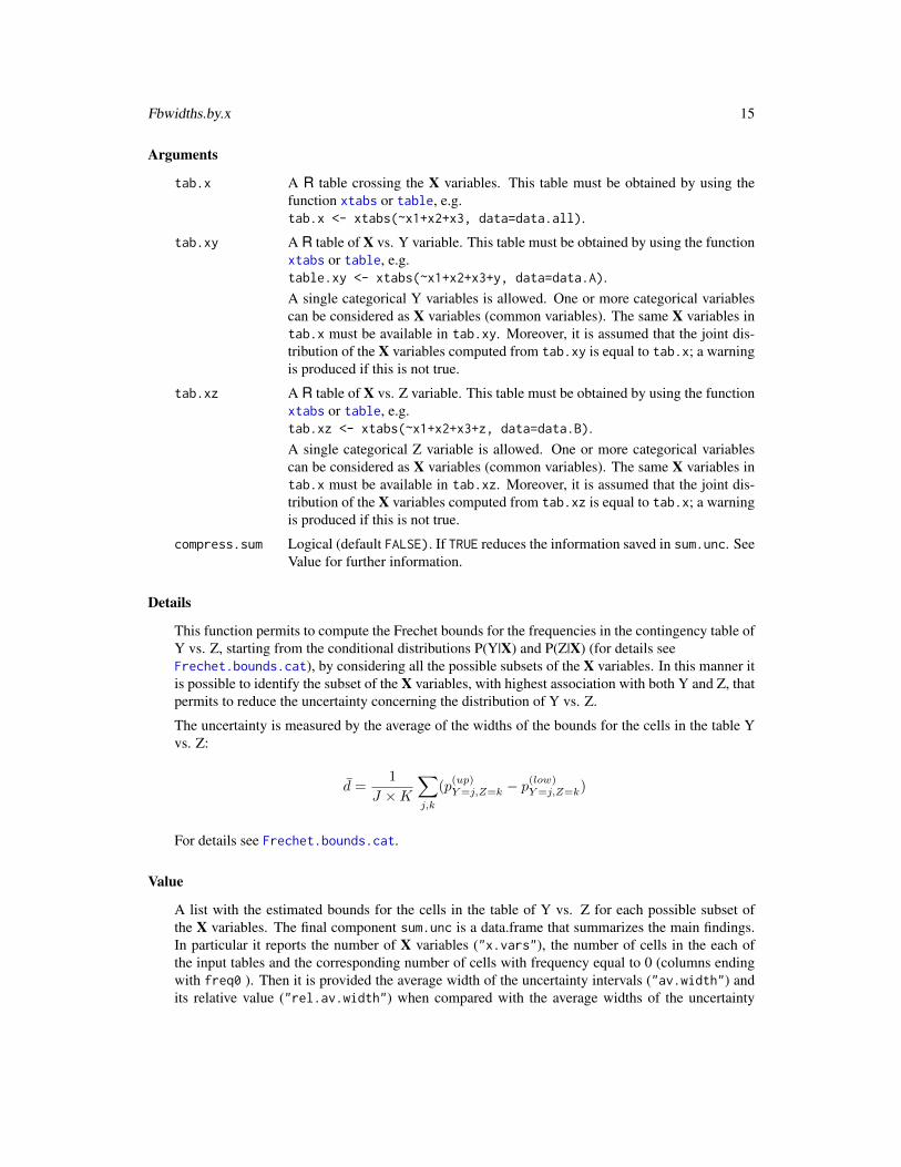
Arguments

tab.x A R table crossing the X variables. This table must be obtained by using thefunction xtabs or table, e.g.tab.x <- xtabs(~x1+x2+x3, data=data.all).

tab.xy A R table of X vs. Y variable. This table must be obtained by using the functionxtabs or table, e.g.table.xy <- xtabs(~x1+x2+x3+y, data=data.A).A single categorical Y variables is allowed. One or more categorical variablescan be considered as X variables (common variables). The same X variables intab.x must be available in tab.xy. Moreover, it is assumed that the joint dis-tribution of the X variables computed from tab.xy is equal to tab.x; a warningis produced if this is not true.

tab.xz A R table of X vs. Z variable. This table must be obtained by using the functionxtabs or table, e.g.tab.xz <- xtabs(~x1+x2+x3+z, data=data.B).A single categorical Z variable is allowed. One or more categorical variablescan be considered as X variables (common variables). The same X variables intab.x must be available in tab.xz. Moreover, it is assumed that the joint dis-tribution of the X variables computed from tab.xz is equal to tab.x; a warningis produced if this is not true.

compress.sum Logical (default FALSE). If TRUE reduces the information saved in sum.unc. SeeValue for further information.

Details

This function permits to compute the Frechet bounds for the frequencies in the contingency table ofY vs. Z, starting from the conditional distributions P(Y|X) and P(Z|X) (for details seeFrechet.bounds.cat), by considering all the possible subsets of the X variables. In this manner itis possible to identify the subset of the X variables, with highest association with both Y and Z, thatpermits to reduce the uncertainty concerning the distribution of Y vs. Z.

The uncertainty is measured by the average of the widths of the bounds for the cells in the table Yvs. Z:

d =1

J ×K∑j,k

(p(up)Y=j,Z=k − p

(low)Y=j,Z=k)

For details see Frechet.bounds.cat.

Value

A list with the estimated bounds for the cells in the table of Y vs. Z for each possible subset ofthe X variables. The final component sum.unc is a data.frame that summarizes the main findings.In particular it reports the number of X variables ("x.vars"), the number of cells in the each ofthe input tables and the corresponding number of cells with frequency equal to 0 (columns endingwith freq0 ). Then it is provided the average width of the uncertainty intervals ("av.width") andits relative value ("rel.av.width") when compared with the average widths of the uncertainty

16 Fbwidths.by.x

intervals when no X variables are considered (i.e. unconditioned "av.width", reported in thefirst row of the data.frame).

When compress.sum = TRUE the data.frame sum.unc will show a combination of the X variablesonly if it determines a reduction of the ("av.width") when compared to the preceding one.

Note that in the presence of too many cells with 0s in the input contingency tables is an indication ofsparseness; this is an unappealing situation when estimating the cells’ relative frequencies needed toderive the bounds; in such cases the corresponding results may be unreliable. A possible alternativeway of working consists in estimating the required parameters by considering a pseudo-Bayes esti-mator (see pBayes); in practice the input tab.x, tab.xy and tab.xz should be the ones providedby the pBayes function.

Author(s)


References

Ballin, M., D’Orazio, M., Di Zio, M., Scanu, M. and Torelli, N. (2009) “Statistical Matching of TwoSurveys with a Common Subset”. Working Paper, 124. Dip. Scienze Economiche e Statistiche,Univ. di Trieste, Trieste.


See Also

Frechet.bounds.cat, harmonize.x

Examples

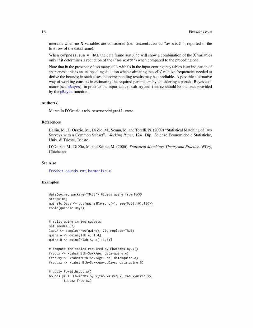
data(quine, package="MASS") #loads quine from MASSstr(quine)quine$c.Days <- cut(quine$Days, c(-1, seq(0,50,10),100))table(quine$c.Days)

# split quine in two subsetsset.seed(4567)lab.A <- sample(nrow(quine), 70, replace=TRUE)quine.A <- quine[lab.A, 1:4]quine.B <- quine[-lab.A, c(1:3,6)]

# compute the tables required by Fbwidths.by.x()freq.x <- xtabs(~Eth+Sex+Age, data=quine.A)freq.xy <- xtabs(~Eth+Sex+Age+Lrn, data=quine.A)freq.xz <- xtabs(~Eth+Sex+Age+c.Days, data=quine.B)

# apply Fbwidths.by.x()bounds.yz <- Fbwidths.by.x(tab.x=freq.x, tab.xy=freq.xy,

tab.xz=freq.xz)

Frechet.bounds.cat 17

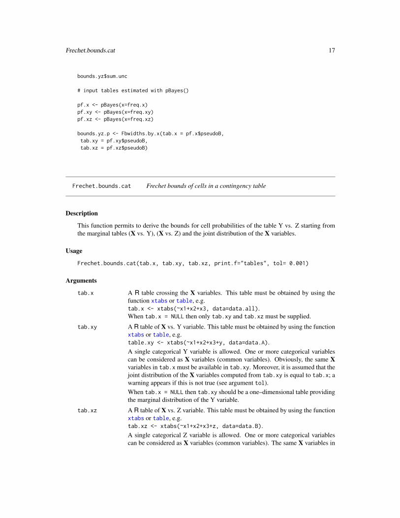
bounds.yz$sum.unc

# input tables estimated with pBayes()

pf.x <- pBayes(x=freq.x)pf.xy <- pBayes(x=freq.xy)pf.xz <- pBayes(x=freq.xz)

bounds.yz.p <- Fbwidths.by.x(tab.x = pf.x$pseudoB,tab.xy = pf.xy$pseudoB,tab.xz = pf.xz$pseudoB)

Frechet.bounds.cat Frechet bounds of cells in a contingency table

Description

This function permits to derive the bounds for cell probabilities of the table Y vs. Z starting fromthe marginal tables (X vs. Y), (X vs. Z) and the joint distribution of the X variables.

Usage

Frechet.bounds.cat(tab.x, tab.xy, tab.xz, print.f="tables", tol= 0.001)

Arguments

tab.x A R table crossing the X variables. This table must be obtained by using thefunction xtabs or table, e.g.tab.x <- xtabs(~x1+x2+x3, data=data.all).When tab.x = NULL then only tab.xy and tab.xz must be supplied.

tab.xy A R table of X vs. Y variable. This table must be obtained by using the functionxtabs or table, e.g.table.xy <- xtabs(~x1+x2+x3+y, data=data.A).A single categorical Y variable is allowed. One or more categorical variablescan be considered as X variables (common variables). Obviously, the same Xvariables in tab.x must be available in tab.xy. Moreover, it is assumed that thejoint distribution of the X variables computed from tab.xy is equal to tab.x; awarning appears if this is not true (see argument tol).When tab.x = NULL then tab.xy should be a one–dimensional table providingthe marginal distribution of the Y variable.

tab.xz A R table of X vs. Z variable. This table must be obtained by using the functionxtabs or table, e.g.tab.xz <- xtabs(~x1+x2+x3+z, data=data.B).A single categorical Z variable is allowed. One or more categorical variablescan be considered as X variables (common variables). The same X variables in

18 Frechet.bounds.cat

tab.x must be available in tab.xz. Moreover, it is assumed that the joint dis-tribution of the X variables computed from tab.xz is equal to tab.x; a warningappears if this is not true (see argument tol).When tab.x = NULL then tab.xz should be a one–dimensional table providingthe marginal distribution of the Z variable.

print.f A string: when print.f="tables" (default) all the cells’ estimates will besaved as tables in a list. On the contrary, if print.f="data.frame", they willbe saved as columns of a data.frame.

tol Tolerance used in comparing joint distributions as far as X variables are consid-ered (default tol= 0.001); the joint distribution of the X variables computedfrom tab.xy and tab.xz should be equal to that in tab.x.

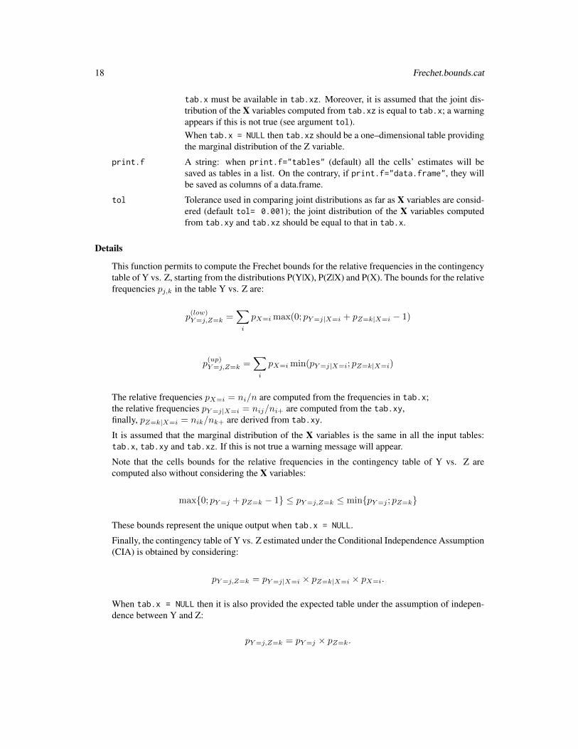
Details

This function permits to compute the Frechet bounds for the relative frequencies in the contingencytable of Y vs. Z, starting from the distributions P(Y|X), P(Z|X) and P(X). The bounds for the relativefrequencies pj,k in the table Y vs. Z are:

p(low)Y=j,Z=k =

∑i

pX=i max(0; pY=j|X=i + pZ=k|X=i − 1)

p(up)Y=j,Z=k =

∑i

pX=i min(pY=j|X=i; pZ=k|X=i)

The relative frequencies pX=i = ni/n are computed from the frequencies in tab.x;the relative frequencies pY=j|X=i = nij/ni+ are computed from the tab.xy,finally, pZ=k|X=i = nik/nk+ are derived from tab.xy.

It is assumed that the marginal distribution of the X variables is the same in all the input tables:tab.x, tab.xy and tab.xz. If this is not true a warning message will appear.

Note that the cells bounds for the relative frequencies in the contingency table of Y vs. Z arecomputed also without considering the X variables:

max{0; pY=j + pZ=k − 1} ≤ pY=j,Z=k ≤ min{pY=j ; pZ=k}

These bounds represent the unique output when tab.x = NULL.

Finally, the contingency table of Y vs. Z estimated under the Conditional Independence Assumption(CIA) is obtained by considering:

pY=j,Z=k = pY=j|X=i × pZ=k|X=i × pX=i.

When tab.x = NULL then it is also provided the expected table under the assumption of indepen-dence between Y and Z:

pY=j,Z=k = pY=j × pZ=k.

Frechet.bounds.cat 19

Note that in the presence of too many cells with 0s in the input contingency tables is an indication ofsparseness; this is an unappealing situation when estimating the cells’ relative frequencies needed toderive the bounds; in such cases the corresponding results may be unreliable. A possible alternativeway of working consists in estimating the required parameters by considering a pseudo-Bayes esti-mator (see pBayes); in practice the input tab.x, tab.xy and tab.xz should be the ones providedby the pBayes function.

Value

When print.f="tables" (default) a list with the following components:

low.u The estimated lower bounds for the relative frequencies in the table Y vs. Zwithout conditioning on the X variables.

up.u The estimated upper bounds for the relative frequencies in the table Y vs. Zwithout conditioning on the X variables.

CIA The estimated relative frequencies in the table Y vs. Z under the ConditionalIndependence Assumption (CIA).

low.cx The estimated lower bounds for the relative frequencies in the table Y vs. Zwhen conditioning on the X variables.

up.cx The estimated upper bounds for the relative frequencies in the table Y vs. Zwhen conditioning on the X variables.

uncertainty The uncertainty associated to input data, summarized in terms of average widthof uncertainty bounds with and without conditioning on the X variables

When print.f="data.frame" the output list contains just two components:

bounds A data.frame whose columns reports the estimated uncertainty bounds.

uncertainty The uncertainty associated to input data, summarized in terms of average widthof uncertainty bounds with and without conditioning on the X variables

Author(s)


References

Ballin, M., D’Orazio, M., Di Zio, M., Scanu, M. and Torelli, N. (2009) “Statistical Matching of TwoSurveys with a Common Subset”. Working Paper, 124. Dip. Scienze Economiche e Statistiche,Univ. di Trieste, Trieste.


See Also

Fbwidths.by.x, harmonize.x

20 Frechet.bounds.cat

Examples


# split quine in two subsetsset.seed(7654)lab.A <- sample(nrow(quine), 70, replace=TRUE)quine.A <- quine[lab.A, 1:3]quine.B <- quine[-lab.A, 2:4]

# compute the tables required by Frechet.bounds.cat()freq.x <- xtabs(~Sex+Age, data=quine.A)freq.xy <- xtabs(~Sex+Age+Eth, data=quine.A)freq.xz <- xtabs(~Sex+Age+Lrn, data=quine.B)

# apply Frechet.bounds.cat()bounds.yz <- Frechet.bounds.cat(tab.x=freq.x, tab.xy=freq.xy,

tab.xz=freq.xz, print.f="data.frame")bounds.yz

#compare marg. distribution of Xs in A and Bcomp.prop(p1=margin.table(freq.xy,c(1,2)), p2=margin.table(freq.xz,c(1,2)),

n1=nrow(quine.A), n2=nrow(quine.B))

# harmonize distr. of Sex vs. Age before applying# Frechet.bounds.cat()

N <- nrow(quine)quine.A$pop <- Nquine.A$f <- N/70 # reciprocal sampling fractionquine.B$pop <- Nquine.B$f <- N/(N-70)

# derive the table of Sex vs. Age related to the whole data settot.sex.age <- colSums(model.matrix(~Sex*Age-1, data=quine))tot.sex.age

# use hamonize.x() to harmonize the Sex vs. Age between# quine.A and quine.B

# create svydesign objectsrequire(survey)svy.qA <- svydesign(~1, weights=~f, fpc=~pop, data=quine.A)svy.qB <- svydesign(~1, weights=~f, fpc=~pop, data=quine.B)

# apply harmonize.xout.hz <- harmonize.x(svy.A=svy.qA, svy.B=svy.qB, form.x=~Sex*Age-1, x.tot=tot.sex.age)

# compute the new tables required by Frechet.bounds.cat()freq.x <- xtabs(out.hz$weights.A~Sex+Age, data=quine.A)freq.xy <- xtabs(out.hz$weights.A~Sex+Age+Eth, data=quine.A)

gower.dist 21

freq.xz <- xtabs(out.hz$weights.B~Sex+Age+Lrn, data=quine.B)

#compare marg. distribution of Xs in A and Bcomp.prop(p1=margin.table(freq.xy,c(1,2)), p2=margin.table(freq.xz,c(1,2)),

n1=nrow(quine.A), n2=nrow(quine.B))

# apply Frechet.bounds.cat()bounds.yz <- Frechet.bounds.cat(tab.x=freq.x, tab.xy=freq.xy,

tab.xz=freq.xz, print.f="data.frame")bounds.yz

gower.dist Computes the Gower’s Distance

Description

This function computes the Gower’s distance (dissimilarity) among units in a dataset or amongobservations in two distinct datasets.

Usage

gower.dist(data.x, data.y=data.x, rngs=NULL, KR.corr=TRUE)

Arguments

data.x A matrix or a data frame containing variables that should be used in the compu-tation of the distance.Columns of mode numeric will be considered as interval scaled variables; columnsof mode character or class factor will be considered as categorical nominalvariables; columns of class ordered will be considered as categorical ordinalvariables and, columns of mode logical will be considered as binary asym-metric variables (see Details for further information).Missing values (NA) are allowed.If only data.x is supplied, the dissimilarities between rows of data.x will becomputed.

data.y A numeric matrix or data frame with the same variables, of the same type, asthose in data.x. Dissimilarities between rows of data.x and rows of data.ywill be computed. If not provided, by default it is assumed equal to data.x andonly dissimilarities between rows of data.x will be computed.

rngs A vector with the ranges to scale the variables. Its length must be equal tonumber of variables in data.x. In correspondence of nonnumeric variables,just put 1 or NA. When rngs=NULL (default) the range of a numeric variable isestimated by jointly considering the values for the variable in data.x and thosein data.y. Therefore, assuming rngs=NULL, if a variable "X1" is considered:

rngs["X1"] <- max(data.x[,"X1"], data.y[,"X1"]) -min(data.x[,"X1"], data.y[,"X1"])

22 gower.dist

.

KR.corr When TRUE (default) the extension of the Gower’s dissimilarity measure pro-posed by Kaufman and Rousseeuw (1990) is used. Otherwise, whenKR.corr=FALSE, the Gower’s (1971) formula is considered.

Details

This function computes distances among records when variables of different type (categorical andcontinuous) have been observed. In order to handle different types of variables, the Gower’s dissim-ilarity coefficient (Gower, 1971) is used. By default (KR.corr=TRUE) the Kaufman and Rousseeuw(1990) extension of the Gower’s dissimilarity coefficient is used.

The final dissimilarity between the ith and jth unit is obtained as a weighted sum of dissimilaritiesfor each variable:

d(i, j) =

∑k δijkdijk∑

k δijk

In particular, dijk represents the distance between the ith and jth unit computed considering the kthvariable. It depends on the nature of the variable:

• logical columns are considered as asymmetric binary variables, for such case dijk = 0 ifxik = xjk = TRUE, 1 otherwise;

• factor or character columns are considered as categorical nominal variables and dijk = 0if xik = xjk, 1 otherwise;

• numeric columns are considered as interval-scaled variables and

dijk =|xik − xjk|

Rk

being Rk the range of the kth variable. The range is the one supplied with the argument rngs(rngs[k]) or the one computed on available data (when rngs=NULL);

• ordered columns are considered as categorical ordinal variables and the values are substitutedwith the corresponding position index, rik in the factor levels. When KR.corr=FALSE theseposition indexes (that are different from the output of the R function rank) are transformed inthe following manner

zik =(rik − 1)

max (rik)− 1

These new values, zik, are treated as observations of an interval scaled variable.

As far as the weight δijk is concerned:

• δijk = 0 if xik = NA or xjk = NA;

• δijk = 0 if the variable is asymmetric binary and xik = xjk = 0 or xik = xjk = FALSE;

• δijk = 1 in all the other cases.

In practice, NAs and couple of cases with xik = xjk = FALSE do not contribute to distance compu-tation.

Value

A matrix object with distances among rows of data.x and those of data.y.

harmonize.x 23

Author(s)


References

Gower, J. C. (1971), “A general coefficient of similarity and some of its properties”. Biometrics,27, 623–637.

Kaufman, L. and Rousseeuw, P.J. (1990), Finding Groups in Data: An Introduction to ClusterAnalysis. Wiley, New York.

See Also

daisy, dist

Examples

x1 <- as.logical(rbinom(10,1,0.5))x2 <- sample(letters, 10, replace=TRUE)x3 <- rnorm(10)x4 <- ordered(cut(x3, -4:4, include.lowest=TRUE))xx <- data.frame(x1, x2, x3, x4, stringsAsFactors = FALSE)

# matrix of distances among observations in xxdx <- gower.dist(xx)head(dx)

# matrix of distances among first obs. in xx# and the remaining onesgower.dist(data.x=xx[1:6,], data.y=xx[7:10,])

harmonize.x Harmonizes the marginal (joint) distribution of a set of variables ob-served independently in two sample surveys referred to the same targetpopulation

Description

This function permits to harmonize the marginal or the joint distribution of a set of variables ob-served independently in two sample surveys carried out on the same target population. This harmo-nization is carried out by using the calibration of the survey weights of the sample units in both thesurveys according to the procedure suggested by Renssen (1998).

Usage

harmonize.x(svy.A, svy.B, form.x, x.tot=NULL,cal.method="linear", ...)

24 harmonize.x

Arguments

svy.A A svydesign R object that stores the data collected in the the survey A and allthe information concerning the sampling design. This object can be created byusing the function svydesign in the package survey.

svy.B A svydesign R object that stores the data collected in the the survey B and allthe information concerning the sampling design. This object can be created byusing the function svydesign in the package survey.

form.x A R formula specifying which of the variables, common to both the surveys,have to be considered, and how have to be considered. For instanceform.x=~x1+x2 means that the marginal distribution of the variables x1 andx2 have to be harmonized and there is also an ‘Intercept’. In order to skip theintercept the formula has to be written in the following mannerform.x=~x1+x2-1.When dealing with categorical variables, if the formula is written in the follow-ing manner form.x=~x1:x2-1 it means that the harmonization has to be carriedout by considering the joint distribution of the two variables (x1 vs. x2). Tobetter understand how form.x works see model.matrix (see also formula).Due to weights calibration features, it is preferable to work with categoricalX variables. In some cases, the procedure may be successful when a singlecontinuous variable is considered jointly with one or more categorical variables.When dealing with several continuous variable it may be preferable to categorizethem.

x.tot A vector or table with known population totals for the X variables. A vector isrequired when cal.method="linear" or cal.method="raking". The namesand the length of the vector depends on the way it is specified the argumentform.x (see model.matrix). A contingency table is required whencal.method="poststratify" (for details see postStratify).When x.tot is not provided (i.e. x.tot=NULL) then the vector of totals is es-timated as a weighted average of the totals estimated on the two surveys. Theweight assigned to the totals estimated from A is λ = nA/(nA + nB); 1 − λis the weight assigned to X totals estimated from survey B (nA and nB are thenumber of units in A and B respectively).

cal.method A string that specifies how the calibration of the weights in svy.A and svy.Bhas to be carried out. By default cal.method="linear" linear calibration isperformed. In particular, the calibration is carried out by mean of the functioncalibrate in the package survey.Alternatively, it is possible to rake the origin survey weights by specifyingcal.method="raking". Finally, it is possible to perform a simple post-stratificationby setting cal.method="poststratify". Note that in this case the weights ad-justments are carried out by considering the functionpostStratify in the package survey.

... Further arguments that may be necessary for calibration or post-stratification. Inparticular, when cal.method="linear" there is the chance of having negativeweights. This drawback can be avoided by requiring that the final weights liein a given interval specified via bounds argument (an argument of calibrate).

harmonize.x 25

In sample surveys one expects that weights are greater than or equal to 1, i.e.bounds=c(1, Inf).The number of iterations used in calibration can be modified too by using theargument maxit (by default maxit=50).See calibrate for further details.

Details

This function harmonizes the totals of the X variables, observed in both survey A and survey B, tobe equal to given known totals specified via x.tot. When these totals are not known (x.tot=NULL)they are estimated by combining the estimates derived from the two separate surveys. The harmo-nization is carried out according to a procedure suggested by Renssen (1998) based on calibration ofsurvey weights (for major details on calibration see Sarndal and Lundstrom, 2005). The procedureis particularly suited to deal with categorical X variables, in this case it permits to harmonize thejoint or the marginal distribution of the categorical variables being considered. Note that an incom-plete crossing of the X variables can be considered: i.e. harmonisation wrt to the joint distributionof X1 ×X2 and the marginal distribution of X3).

The calibration procedure may not produce the final result due to convergence problems. In this casean error message appears. In order to reach convergence it may be necessary to launch the procedurewith less constraints (i.e a reduced number of population totals) by joining adjacent categories orby discarding some variables.

In some limited cases it could be possible to consider both categorical and continuous variables. Inthis situation it may happen that calibration is not successful. In order to reach convergence it maybe necessary to categorize the continuous X variables.

Post-stratification is a special case of calibration; all the weights of the units in a given post-stratumare modified so the reproduce the known total for that post-stratum. Post-stratification avoids prob-lems of convergence but, on the other hand it may produce final weights with a higher variabilitythan those derived from the calibration.

Value

A R with list the results of calibration procedures carried out on survey A and survey B, respectively.In particular the following components will be provided:

cal.A The survey object svy.A after the calibration; in particular, the weights now arecalibrated with respect to the totals of the X variables.

cal.B The survey object svy.B after the calibration; in particular, the weights now arecalibrated with respect to the totals of the X variables.

weights.A The new calibrated weights associated to the the units in svy.A.

weights.B The new calibrated weights associated to the the units in svy.B.

call Stores the call to this function with all the values specified for the various argu-ments (call=match.call()).

Author(s)


26 harmonize.x

References


Renssen, R.H. (1998) “Use of Statistical Matching Techniques in Calibration Estimation”. SurveyMethodology, N. 24, pp. 171–183.

Sarndal, C.E. and Lundstrom, S. (2005) Estimation in Surveys with Nonresponse. Wiley, Chichester.

See Also

comb.samples, calibrate, svydesign, postStratify,

Examples


# split quine in two subsetsset.seed(7654)lab.A <- sample(nrow(quine), 70, replace=TRUE)quine.A <- quine[lab.A, c("Eth","Sex","Age","Lrn")]quine.B <- quine[-lab.A, c("Eth","Sex","Age","Days")]

# create svydesign objectsrequire(survey)quine.A$f <- 70/nrow(quine) # sampling fractionquine.B$f <- (nrow(quine)-70)/nrow(quine)svy.qA <- svydesign(~1, fpc=~f, data=quine.A)svy.qB <- svydesign(~1, fpc=~f, data=quine.B)

#------------------------------------------------------# example (1)# Harmonizazion of the distr. of Sex vs. Age# usign poststratification

# (1.a) known population totals# the population toatal are computed on the full data frametot.sex.age <- xtabs(~Sex+Age, data=quine)tot.sex.age

out.hz <- harmonize.x(svy.A=svy.qA, svy.B=svy.qB, form.x=~Sex+Age,x.tot=tot.sex.age, cal.method="poststratify")

tot.A <- xtabs(out.hz$weights.A~Sex+Age, data=quine.A)tot.B <- xtabs(out.hz$weights.B~Sex+Age, data=quine.B)

tot.sex.age-tot.Atot.sex.age-tot.B

# (1.b) unknown population totals (x.tot=NULL)# the population total is estimated by combining totals from the

harmonize.x 27

# two surveys

out.hz <- harmonize.x(svy.A=svy.qA, svy.B=svy.qB, form.x=~Sex+Age,x.tot=NULL, cal.method="poststratify")

tot.A <- xtabs(out.hz$weights.A~Sex+Age, data=quine.A)tot.B <- xtabs(out.hz$weights.B~Sex+Age, data=quine.B)

tot.Atot.A-tot.B

#-----------------------------------------------------# example (2)# Harmonizazion wrt the maginal distribution# of 'Eth', 'Sex' and 'Age'# using linear calibration

# (2.a) vector of population total known# estimated from the full data set# note the formula! only marginal distribution of the# variables are consideredtot.m <- colSums(model.matrix(~Eth+Sex+Age-1, data=quine))tot.m

out.hz <- harmonize.x(svy.A=svy.qA, svy.B=svy.qB, x.tot=tot.m,form.x=~Eth+Sex+Age-1, cal.method="linear")

summary(out.hz$weights.A) #check for negative weightssummary(out.hz$weights.B) #check for negative weights

tot.msvytable(formula=~Eth, design=out.hz$cal.A)svytable(formula=~Eth, design=out.hz$cal.B)

svytable(formula=~Sex, design=out.hz$cal.A)svytable(formula=~Sex, design=out.hz$cal.B)

# Note: margins are equal but joint distributions are not!svytable(formula=~Sex+Age, design=out.hz$cal.A)svytable(formula=~Sex+Age, design=out.hz$cal.B)

# (2.b) vector of population total unknownout.hz <- harmonize.x(svy.A=svy.qA, svy.B=svy.qB, x.tot=NULL,

form.x=~Eth+Sex+Age-1, cal.method="linear")svytable(formula=~Eth, design=out.hz$cal.A)svytable(formula=~Eth, design=out.hz$cal.B)

svytable(formula=~Sex, design=out.hz$cal.A)svytable(formula=~Sex, design=out.hz$cal.B)

#-----------------------------------------------------# example (3)# Harmonizazion wrt the joint distribution of 'Sex' vs. 'Age'

28 mahalanobis.dist

# and the marginal distribution of 'Eth'# using raking

# vector of population total known# estimated from the full data set# note the formula!tot.m <- colSums(model.matrix(~Eth+(Sex:Age-1)-1, data=quine))tot.m

out.hz <- harmonize.x(svy.A=svy.qA, svy.B=svy.qB, x.tot=tot.m,form.x=~Eth+(Sex:Age)-1, cal.method="raking")

summary(out.hz$weights.A) #check for negative weightssummary(out.hz$weights.B) #check for negative weights

tot.msvytable(formula=~Eth, design=out.hz$cal.A)svytable(formula=~Eth, design=out.hz$cal.B)

svytable(formula=~Sex+Age, design=out.hz$cal.A)svytable(formula=~Sex+Age, design=out.hz$cal.B)

#-----------------------------------------------------# example (4)# Harmonizazion wrt the joint distribution# of ('Sex' x 'Age' x 'Eth')

# vector of population total known# estimated from the full data set# note the formula!tot.m <- colSums(model.matrix(~Eth:Sex:Age-1, data=quine))tot.m

out.hz <- harmonize.x(svy.A=svy.qA, svy.B=svy.qB, x.tot=tot.m,form.x=~Eth:Sex:Age-1, cal.method="linear")

tot.msvytable(formula=~Eth+Sex+Age, design=out.hz$cal.A)svytable(formula=~Eth+Sex+Age, design=out.hz$cal.B)

mahalanobis.dist Computes the Mahalanobis Distance

Description

This function computes the Mahalanobis distance among units in a dataset or among observationsin two distinct datasets.

Usage

mahalanobis.dist(data.x, data.y=NULL, vc=NULL)

mahalanobis.dist 29

Arguments

data.x A matrix or a data frame containing variables that should be used in the com-putation of the distance. Only continuous variables are allowed. Missing values(NA) are not allowed.

When only data.x is supplied, the distances between rows of data.x is com-puted.

data.y A numeric matrix or data frame with the same variables, of the same type, asthose in data.x (only continuous variables are allowed). Dissimilarities be-tween rows of data.x and rows of data.y will be computed. If not provided,by default it is assumed data.y=data.x and only dissimilarities between rowsof data.x will be computed.

vc Covariance matrix that should be used in distance computation. If it is notsupplied (vc=NULL) it is estimated from the input data. In particular, whenvc=NULL and only data.x is supplied then the covariance matrix is estimatedfrom data.x (var(data.x)). On the contrary when vc=NULL and both data.xand data.y are available then the covariance matrix is estimated on the joineddata sets (i.e. var(rbind(data.x, data.y))).

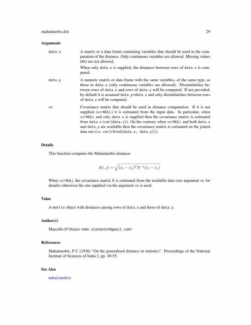
Details

This function computes the Mahalanobis distance:

d(i, j) =√

(xi − xj)TS−1(xi − xj)

When vc=NULL the covariance matrix S is estimated from the available data (see argument vc fordetails) otherwise the one supplied via the argument vc is used.

Value


Author(s)


References

Mahalanobis, P C (1936) “On the generalised distance in statistics”. Proceedings of the NationalInstitute of Sciences of India 2, pp. 49-55.

See Also

mahalanobis

30 maximum.dist

Examples

md1 <- mahalanobis.dist(iris[1:6,1:4])md2 <- mahalanobis.dist(data.x=iris[1:6,1:4], data.y=iris[51:60, 1:4])

vv <- var(iris[,1:4])md1a <- mahalanobis.dist(data.x=iris[1:6,1:4], vc=vv)md2a <- mahalanobis.dist(data.x=iris[1:6,1:4], data.y=iris[51:60, 1:4], vc=vv)

maximum.dist Computes the Maximum Distance

Description

This function computes the Maximum distance (or L∞ norm) among units in a dataset or amongobservations in two distinct datasets.

Usage

maximum.dist(data.x, data.y=data.x, rank=FALSE)

Arguments

data.x A matrix or a data frame containing variables that should be used in the com-putation of the distance. Only continuous variables are allowed. Missing values(NA) are not allowed.When only data.x is supplied, the distances between rows of data.x is com-puted.

data.y A numeric matrix or data frame with the same variables, of the same type, asthose in data.x (only continuous variables are allowed). Dissimilarities be-tween rows of data.x and rows of data.y will be computed. If not provided,by default it is assumed data.y=data.x and only dissimilarities between rowsof data.x will be computed.

rank Logical, when TRUE the original values are substituted by their ranks dividedby the number of values plus one (following suggestion in Kovar et al. 1988).This rank transformation permits to remove the effect of different scales on thedistance computation. When computing ranks the tied observations assume theaverage of their position (ties.method = "average" in calling the rank func-tion).

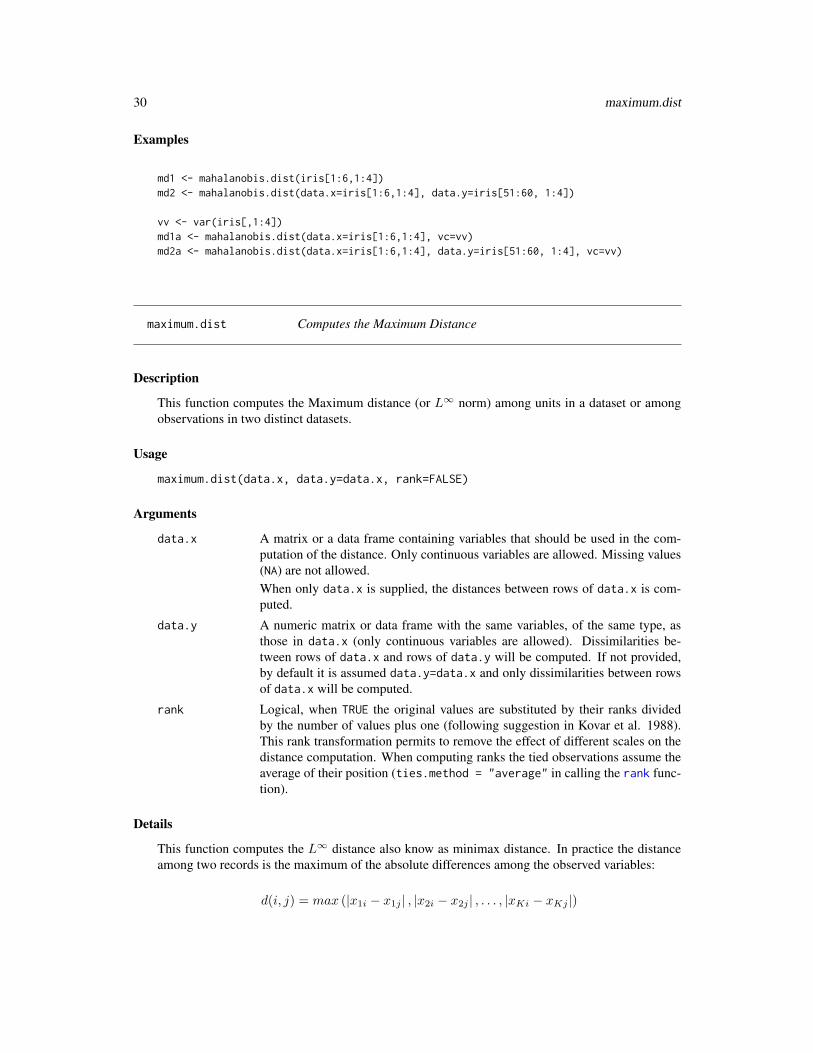
Details

This function computes the L∞ distance also know as minimax distance. In practice the distanceamong two records is the maximum of the absolute differences among the observed variables:

d(i, j) = max (|x1i − x1j | , |x2i − x2j | , . . . , |xKi − xKj |)

mixed.mtc 31

When rank=TRUE the original values are substituted by their ranks divided by the number of valuesplus one (following suggestion in Kovar et al. 1988).

Value


Author(s)


References

Kovar, J.G., MacMillan, J. and Whitridge, P. (1988). “Overview and strategy for the GeneralizedEdit and Imputation System”. Statistics Canada, Methodology Branch Working Paper No. BSMD88-007 E/F.

See Also

rank,

Examples

md1 <- maximum.dist(iris[1:10,1:4])md2 <- maximum.dist(iris[1:10,1:4], rank=TRUE)

md3 <- maximum.dist(data.x=iris[1:50,1:4], data.y=iris[51:100,1:4])md4 <- maximum.dist(data.x=iris[1:50,1:4], data.y=iris[51:100,1:4], rank=TRUE)

mixed.mtc Statistical Matching via Mixed Methods

Description

This function implements some mixed methods to perform statistical matching between two datasources.

Usage

mixed.mtc(data.rec, data.don, match.vars, y.rec, z.don, method="ML",rho.yz=NULL, micro=FALSE, constr.alg="Hungarian")

32 mixed.mtc

Arguments

data.rec A matrix or data frame that plays the role of recipient in the statistical matchingapplication. This data set must contain all variables (columns) that should beused in statistical matching, i.e. the variables called by the argumentsmatch.vars and y.rec. Note that continuous variables are expected, if thereare some categorical variables they are recoded into dummies. Missing values(NA) are not allowed.

data.don A matrix or data frame that plays the role of donor in the statistical matchingapplication. This data set must contain all the numeric variables (columns) thatshould be used in statistical matching, i.e. the variables called by the argumentsmatch.vars and z.don. Note that continuous variables are expected, if thereare some categorical variables they are recoded into dummies. Missing values(NA) are not allowed.

match.vars A character vector with the names of the common variables (the columns in boththe data frames) to be used as matching variables (X).

y.rec A character vector with the name of the target variable Y that is observed onlyfor units in data.rec. Only one continuous variable is allowed.

z.don A character vector with the name of the target variable Z that is observed onlyfor units in data.don. Only one continuous variable is allowed.

method A character vector that identifies the method that should be used to estimatethe parameters of the regression models: Y vs. X and Z vs. X. MaximumLikelihood method is used when method="ML" (default); on the contrary, whenmethod="MS" the parameters are estimated according to approach proposed byMoriarity and Scheuren (2001 and 2003). See Details for further information.

rho.yz A numeric value representing a guess for the correlation among the Y (y.rec)and the Z variable (z.don) that are not jointly observed. When method="MS"then the argument cor.yz must specify the value of the correlation coefficientρY Z ; on the contrary, when method="ML", it must specify the partial correlationcoefficient among Y and Z given X (ρY Z|X).By default (rho.yz=NULL). In practice, in absence of auxiliary information con-cerning the correlation coefficient or the partial correlation coefficient, the sta-tistical matching is carried out under the assumption of independence among Yand Z given X (Conditional Independence Assumption, CIA ), i.e. ρY Z|X = 0.

micro Logical. When micro=FALSE (default) only the parameter estimates are re-turned. On the contrary, when micro=TRUE the function returns also data.recfilled in with the values for the variable Z. The donors for filling in Z in data.recare identified using a constrained distance hot deck method. In this case, thenumber of units (rows) in data.don must be grater or equal to the number ofunits (rows) in data.rec. See next argument and Details for further informa-tion.

constr.alg A string that has to be specified when micro=TRUE, in order to solve the trans-portation problem involved by the constrained distance hot deck method. Twochoices are available: “lpSolve” and “Hungarian”. In the first case,constr.alg="lpSolve", the transportation problem is solved by means of thefunction lp.transport available in the package lpSolve. When

mixed.mtc 33

constr.alg="Hungarian" (default) the transportation problem is solved usingthe Hungarian method implemented in the function solve_LSAP available in thepackage clue (Hornik, 2012). Note that Hungarian algorithm is more efficientand requires less processing time.

Details

This function implements some mixed methods to perform statistical matching. A mixed methodconsists of two steps:

(1) adoption of a parametric model for the joint distribution of (X, Y, Z) and estimation of itsparameters;

(2) derivation of a complete “synthetic” data set (recipient data set filled in with values for the Zvariable) using a nonparametric approach.

In this case, as far as (1) is concerned, it is assumed that (X, Y, Z) follows a multivariate normaldistribution. Please note that if some of the X are categorical, then they are recoded into dummiesbefore starting with the estimation. In such a case the assumption of multivariate normal distributionmay be questionable.

The whole procedure is based on the imputation method known as predictive mean matching. Theprocedure consists of three steps:

step 1a) Regression step: the two linear regression models Y vs. X and Z vs. X are considered andtheir parameters are estimated.

step 1b) Computation of intermediate values. For the units in data.rec the following intermediatevalues are derived:

za = αZ + βZXxa + ea

for each a = 1, . . . , nA, being nA the number of units in data.rec (rows of data.rec). Notethat, ea is a random draw from the multivariate normal distribution with zero mean and estimatedresidual variance σZ|X.

Similarly, for the units in data.don the following intermediate values are derived:

yb = αY + βYXxb + eb

for each b = 1, . . . , nB , being nB the number of units in data.don (rows of data.don). eb isa random draw from the multivariate normal distribution with zero mean and estimated residualvariance σY |X.

step 2) Matching step. For each observation (row) in data.rec a donor is chosen in data.donthrough a nearest neighbor constrained distance hot deck procedure. The distances are computedbetween (ya, za) and (yb, zb) using Mahalanobis distance.

For further details see Sections 2.5.1 and 3.6.1 in D’Orazio et al. (2006).

In step 1a) the parameters of the regression model can be estimated by means of the MaximumLikelihood method (method="ML") (see D’Orazio et al., 2006, pp. 19–23,73–75) or, using theMoriarity and Scheuren (2001 and 2003) approach (method="MS") (see also D’Orazio et al., 2006,pp. 75–76). The two estimation methods are compared in D’Orazio et al. (2005).

34 mixed.mtc

When method="MS", if the value specified for the argument rho.yz is not compatible with theother correlation coefficients estimated from the data, then it is substituted with the closest valuecompatible with the other estimated coefficients.

When micro=FALSE only the estimation of the parameters is performed (step 1a). Otherwise,(micro=TRUE) the whole procedure is carried out.

Value

A list with a varying number of components depending on the values of the arguments method andrho.yz.

mu The estimated mean vector.

vc The estimated variance–covariance matrix.

cor The estimated correlation matrix.

res.var A vector with estimates of the residual variances σY |ZX and σZ|YX.

start.prho.yz It is the initial guess for the partial correlation coefficient ρY Z|X passed in inputvia the rho.yz argument when method="ML".

rho.yz Returned in output only when method="MS". It is a vector with four values:the initial guess for ρY Z ; the lower and upper bounds for ρY Z in the statisti-cal matching framework given the correlation coefficients among Y and X andthe correlation coefficients among Z and X estimated from the available data;and, finally, the closest admissible value used in computations instead of theinitial rho.yz that resulted not coherent with the others correlation coefficientsestimated from the available data.

phi When method="MS". Estimates of the φ terms introduced by Moriarity andScheuren (2001 and 2003).

filled.rec The data.rec filled in with the values of Z. It is returned only whenmicro=TRUE.

mtc.ids when micro=TRUE. This is a matrix with the same number of rows of data.recand two columns. The first column contains the row names of the data.recand the second column contains the row names of the corresponding donorsselected from the data.don. When the input matrices do not contain row names,a numeric matrix with the indexes of the rows is provided.

dist.rd A vector with the distances among each recipient unit and the correspondingdonor, returned only in case micro=TRUE.

call How the function has been called.

Author(s)


References

D’Orazio, M., Di Zio, M. and Scanu, M. (2005). “A comparison among different estimators ofregression parameters on statistically matched files through an extensive simulation study”, Con-tributi, 2005/10, Istituto Nazionale di Statistica, Rome.

mixed.mtc 35


Hornik K. (2012). clue: Cluster ensembles. R package version 0.3-45. https://CRAN.R-project.org/package=clue.

Moriarity, C., and Scheuren, F. (2001). “Statistical matching: a paradigm for assessing the un-certainty in the procedure”. Journal of Official Statistics, 17, 407–422. http://www.jos.nu/Articles/abstract.asp?article=173407

Moriarity, C., and Scheuren, F. (2003). “A note on Rubin’s statistical matching using file concatena-tion with adjusted weights and multiple imputation”, Journal of Business and Economic Statistics,21, 65–73.

See Also

NND.hotdeck, mahalanobis.dist

Examples

# reproduce the statistical matching framework# starting from the iris data.frameset.seed(98765)pos <- sample(1:150, 50, replace=FALSE)ir.A <- iris[pos,c(1,3:5)]ir.B <- iris[-pos, 2:5]

xx <- intersect(colnames(ir.A), colnames(ir.B))xx # common variables

# ML estimation method under CIA ((rho_YZ|X=0));# only parameter estimates (micro=FALSE)# only continuous matching variablesxx.mtc <- c("Petal.Length", "Petal.Width")mtc.1 <- mixed.mtc(data.rec=ir.A, data.don=ir.B, match.vars=xx.mtc,

y.rec="Sepal.Length", z.don="Sepal.Width")

# estimated correlation matrixmtc.1$cor

# ML estimation method under CIA ((rho_YZ|X=0));# only parameter estimates (micro=FALSE)# categorical variable 'Species' used as matching variable

xx.mtc <- xxmtc.2 <- mixed.mtc(data.rec=ir.A, data.don=ir.B, match.vars=xx.mtc,

y.rec="Sepal.Length", z.don="Sepal.Width")


# ML estimation method with partial correlation coefficient

https://CRAN.R-project.org/package=clue


http://www.jos.nu/Articles/abstract.asp?article=173407

http://www.jos.nu/Articles/abstract.asp?article=173407

36 mixed.mtc

# set equal to 0.5 (rho_YZ|X=0.5)# only parameter estimates (micro=FALSE)

mtc.3 <- mixed.mtc(data.rec=ir.A, data.don=ir.B, match.vars=xx.mtc,y.rec="Sepal.Length", z.don="Sepal.Width",rho.yz=0.5)


# ML estimation method with partial correlation coefficient# set equal to 0.5 (rho_YZ|X=0.5)# with imputation step (micro=TRUE)

mtc.4 <- mixed.mtc(data.rec=ir.A, data.don=ir.B, match.vars=xx.mtc,y.rec="Sepal.Length", z.don="Sepal.Width",rho.yz=0.5, micro=TRUE, constr.alg="Hungarian")

# first rows of data.rec filled in with zhead(mtc.4$filled.rec)

## Moriarity and Scheuren estimation method under CIA;# only with parameter estimates (micro=FALSE)mtc.5 <- mixed.mtc(data.rec=ir.A, data.don=ir.B, match.vars=xx.mtc,

y.rec="Sepal.Length", z.don="Sepal.Width",method="MS")

# the starting value of rho.yz and the value used# in computationsmtc.5$rho.yz


# Moriarity and Scheuren estimation method# with correlation coefficient set equal to -0.15 (rho_YZ=-0.15)# with imputation step (micro=TRUE)

mtc.6 <- mixed.mtc(data.rec=ir.A, data.don=ir.B, match.vars=xx.mtc,y.rec="Sepal.Length", z.don="Sepal.Width",method="MS", rho.yz=-0.15,micro=TRUE, constr.alg="lpSolve")

# the starting value of rho.yz and the value used# in computationsmtc.6$rho.yz


# first rows of data.rec filled in with z imputed valueshead(mtc.6$filled.rec)

NND.hotdeck 37

NND.hotdeck Distance Hot Deck method.

Description

This function implements the distance hot deck method to match the records of two data sourcesthat share some variables.

Usage

NND.hotdeck(data.rec, data.don, match.vars,don.class=NULL, dist.fun="Manhattan",constrained=FALSE, constr.alg="Hungarian",k=1, keep.t=FALSE, ...)

Arguments

data.rec A matrix or data frame that plays the role of recipient. This data frame mustcontain the variables (columns) that should be used, directly or indirectly, in thematching application (specified via match.vars and eventually don.class).Missing values (NA) are allowed.

data.don A matrix or data frame that plays the role of donor. The variables (columns)involved, directly or indirectly, in the computation of distance must be the sameand of the same type as those in data.rec (specified via match.vars and even-tually don.class).

match.vars A character vector with the names of the matching variables (the columns inboth the data frames) that have to be used to compute distances among records(rows) in data.rec and those in data.don. The variables used in computingdistances may cointain missing values but in this case a limited number of dis-tance functions can be used (see Details for clarifications).

don.class A character vector with the names of the variables (columns in both the dataframes) that have to be used to identify the donation classes. In this case thecomputation of distances is limited to those units of data.rec and data.docthat belong to the same donation class. The case of empty donation classesshould be avoided. It would be preferable that variables used to form donationclasses are defined as factor.The variables chosen for the creation of the donation clasess should not containmissing values (NAs).When not specified (default) no donation classes are used. This choice may re-quire more memory to store a larger distance matrix and a higher computationaleffort.

38 NND.hotdeck

dist.fun A string with the name of the distance function that has to be used. The fol-lowing distances are allowed: “Manhattan” (aka “City block”; default), “Eu-clidean”, “Mahalanobis”,“exact” or “exact matching”, “Gower”, “minimax” orone of the distance functions available in the package proxy. Note that thedistance is computed using the function dist of the package proxy with the ex-ception of the “Gower” (see function gower.dist for details), “Mahalanobis”(function mahalanobis.dist) and “minimax” (see maximum.dist) cases.When dist.fun="Manhattan", "Euclidean", "Mahalanobis" or "minimax"all the non numeric variables in data.rec and data.don will be converted to nu-meric. On the contrary, when dist.fun="exact" or dist.fun="exact matching",all the variables in data.rec and data.don will be converted to character and,as far as the distance computation is concerned, they will be treated as categor-ical nominal variables, i.e. distance is 0 if a couple of units presents the sameresponse category and 1 otherwise.

constrained Logical. When constrained=FALSE (default) each record in data.don can beused as a donor more than once. On the contrary, whenconstrained=TRUE each record in data.don can be used as a donor only ktimes. In this case, the set of donors is selected by solving an optimizationproblem, in order to minimize the overall matching distance. See description ofthe argument constr.alg for details.

constr.alg A string that has to be specified when constrained=TRUE. Two choices areavailable: “lpSolve” and “hungarian”. In the first case, constr.alg="lpSolve",the optimization problem is solved by means of the function lp.transportavailable in the package lpSolve. When constr.alg="hungarian" (default)the problem is solved using the Hungarian method, implemented in functionsolve_LSAP available in the package clue. Note that Hungarian algorithm isfaster and more efficient if compared to constr.alg="lpSolve" but it allowsselecting a donor just once, i.e. k = 1 .

k The number of times that a unit in data.don can be selected as a donor whenconstrained=TRUE (default k = 1 ). When k>1 then optimization problem canbe solved by setting constr.alg="lpSolve". Hungarian algorithm (constr.alg="hungarian")can be used only when k = 1.

keep.t Logical, when donation classes are used by setting keep.t=TRUE prints infor-mation on the donation classes being processed (by default keep.t=FALSE).

... Additional arguments that may be required by gower.dist, or bymaximum.dist, or by dist.

Details

This function finds a donor record in data.don for each record in data.rec. In the unconstrainedcase, it searches for the closest donor record in data.don for each record in the recipient data set,according to the chosen distance function. When for a given recipient record there are more donorsavailable at the minimum distance, one of them is picked at random.

In the constrained case a donor can be used just a fixed number of times, as specified by the kargument, but the whole set of donors is chosen in order to minimize the overall matching distance.When k=1 the number of units (rows) in the donor data set has to be larger or equal to the numberof units of the recipient data set; when the donation classes are used, this condition must be satisfied

NND.hotdeck 39

in each donation class. For further details on nearest neighbor distance hot deck refer to Chapter 2in D’Orazio et al. (2006).

This function can also be used to impute missing values in a data set using the nearest neighbordistance hot deck. In this case data.rec is the part of the initial data set that contains missingvalues; on the contrary, data.don is the part of the data set without missing values. See R code inthe Examples for details.

Please note that only “Gower” and “minimax” distance functions allow for the presence of missingvalues (NAs) in the variables used in computing distances. In both the cases when one of the of theobservations presents a variable showing an NA, then this variable is excluded from the computationof distance.

Value

A R list with the following components:

mtc.ids A matrix with the same number of rows of data.rec and two columns. The firstcolumn contains the row names of the data.rec and the second column containsthe row names of the corresponding donors selected from the data.don. Whenthe input matrices do not contain row names, a numeric matrix with the indexesof the rows is provided.

dist.rd A vector with the distances among each recipient unit and the correspondingdonor.

noad When constrained=FALSE, it reports the number of available donors at theminimum distance for each recipient unit.


Author(s)


References


Hornik K. (2012). clue: Cluster ensembles. R package version 0.3-45. https://CRAN.R-project.org/package=clue.

Rodgers, W.L. (1984). “An evaluation of statistical matching”. Journal of Business and EconomicStatistics, 2, 91–102.

Singh, A.C., Mantel, H., Kinack, M. and Rowe, G. (1993). “Statistical matching: use of auxiliaryinformation as an alternative to the conditional independence assumption”. Survey Methodology,19, 59–79.

See Also

RANDwNND.hotdeck



40 NND.hotdeck

Examples

# reproduce the classical matching frameworklab <- c(1:15, 51:65, 101:115)iris.rec <- iris[lab, c(1:3,5)] # recipient data.frameiris.don <- iris[-lab, c(1:2,4:5)] #donor data.frame

# Now iris.rec and iris.don have the variables# "Sepal.Length", "Sepal.Width" and "Species"# in common.# "Petal.Length" is available only in iris.rec# "Petal.Width" is available only in iris.don

# Find the closest donors donors computing distance# on "Sepal.Length" and "Sepal.Width"# unconstrained case, Euclidean distance

out.NND.1 <- NND.hotdeck(data.rec=iris.rec, data.don=iris.don,match.vars=c("Sepal.Length", "Sepal.Width") )

# create the synthetic data.set:# fill in "Petal.Width" in iris.rec

fused.1 <- create.fused(data.rec=iris.rec, data.don=iris.don,mtc.ids=out.NND.1$mtc.ids, z.vars="Petal.Width")

# Find the closest donors computing distance# on "Sepal.Length", "Sepal.Width" and Species;# unconstrained case, Gower's distance

out.NND.2 <- NND.hotdeck(data.rec=iris.rec, data.don=iris.don,match.vars=c("Sepal.Length", "Sepal.Width", "Species"),dist.fun="Gower")

# find the closest donors using "Species" to form donation classes# and "Sepal.Length" and "Sepal.Width" to compute distance;# unconstrained case.

out.NND.3 <- NND.hotdeck(data.rec=iris.rec, data.don=iris.don,match.vars=c("Sepal.Length", "Sepal.Width"),don.class="Species")

# find the donors using "Species" to form donation classes# and "Sepal.Length" and "Sepal.Width" to compute distance;# constrained case, "Hungarian" algorithm

library(clue)out.NND.4 <- NND.hotdeck(data.rec=iris.rec, data.don=iris.don,

pBayes 41

match.vars=c("Sepal.Length", "Sepal.Width"),don.class="Species", constrained=TRUE,constr.alg="Hungarian")

# Example of Imputation of missing values.# Introducing missing values in irisir.mat <- irismiss <- rbinom(nrow(iris), 1, 0.3)ir.mat[miss==1,"Sepal.Length"] <- NAiris.rec <- ir.mat[miss==1,-1]iris.don <- ir.mat[miss==0,]

#search for NND donorsimp.NND <- NND.hotdeck(data.rec=iris.rec, data.don=iris.don,

match.vars=c("Sepal.Width","Petal.Length", "Petal.Width"),don.class="Species")

# imputing missing valuesiris.rec.imp <- create.fused(data.rec=iris.rec, data.don=iris.don,

mtc.ids=imp.NND$mtc.ids, z.vars="Sepal.Length")

# rebuild the imputed data.framefinal <- rbind(iris.rec.imp, iris.don)

pBayes Pseudo-Bayes estimates of cell probabilities

Description

Estimation of cells counts using the pseudo-Bayes estimator.

Usage

pBayes(x, method="m.ind", const=NULL)

Arguments

x A contingency table with observed cell counts. Typically the output of table orxtabs. More in general an R array with the counts.

method The method for estimating the final cell frequencies. The following options areavailable:method = "Jeffreys", consists in adding 0.5 to each cell before estimation ofthe relative frequencies, in particular the final relative frequencies are derived bymeans of pi = (ni + 0.5)/(n+ c/2), being n the sum of all the counts and c thenumber of cells in the table. The final estimated cell frequencies are obtained asni = n× pi.

42 pBayes

method = "minimax", consists in adding√

(n)/c to each cell before estimationof the relative frequencies, in particular the final relative frequencies are derivedby means of pi = (ni + sqrt(n)/c)/(n+ sqrt(n)).method = "invcat", consists in adding 1/c to each cell before estimation ofthe relative frequencies, in particular the final relative frequencies are derived bymeans of pi = (ni + 1/c)/(n+ 1).method = "user", consists in adding a used defined constant a (a > 0) to eachcell before estimation of the relative frequencies with pi = (ni +a/c)/(n+a×c). The constant a should be passed via the argument const.method = "m.ind", the prior guess for the unknown cell probabilities is ob-tained by considering estimated probabilities under the mutual independencehypothesis. In such a case a data driven K is considered (see Details). Thisoption is available when dealing with at least two-way contingency tables(length(dim(x))>=2).method = "h.assoc", the prior guess for the unknown cell probabilities isobtained by considering estimated probabilities under the homogeneous asso-ciation hypothesis. In such a case a data drive K is considered (see Details).This option is available when dealing with at least two-way contingency tables(length(dim(x))>=2).

const Numeric value, a user defined constant a (a > 0) added to each cell beforeestimation of the relative frequencies when method = "user". As a generalrule of thumb it is preferable to avoid that the sum of constant over all the cellsin table is greater than 0.20× n.

Details

This function estimates the frequencies in a contingency table by using the pseudo-Bayes approach.In practice the estimator being considered is a weighted average of the observed cell counts nh anda suitable prior guess for cell probabilities γh:

ph =n

n+Kph +

K

n+Kγh

K depends on the parameters of Dirichilet prior distribution being considered (for major details seeChapter 12 in Bishop et al., 1974). It is worth noting that with a constant prior guess γh = 1/c(h = 1, 2, · · · , c), setting K = 1 corresponds to adding 1/c to each cell before estimation ofthe relative frequencies (method = "invcat"); with K = c/2 the constant 0.5 is added to eachcell (method = "Jeffreys"); finally when K =

√n the quantity

√n/c is added to each cell

(method = "minimax"). All these cases corresponds to adding a flattening constant; the higher isthe value of K the more the estimates will be shrinked towards γh = 1/c (flattening).

When method = "m.ind" the prior guess γh is estimated under the hypothesis of mutual inde-pendence between the variables crossed in the initial contingency table x, supposed to be at least atwo-way table. In this case the value of K is estimated via a data driven approach by considering

K =1−

∑h p

2h∑

h (γh − ph)2

pBayes 43

On the contrary, when method = "h.assoc" the prior guess γh is estimated under the hypothesisof homogeneous association between the variables crossed in the initial contingency table x.

Please note that when the input table is estimated from sample data where a weight is assigned toeach unit, the weights should e used in estimation of the input table but it is suggested to rescalethem so that they sum up to n, the sample size.

Value

A list object with three components.

invo A vector with the sample size "n", the number of cells ("no.cells") in x, theaverage cell frequency ("av.cfr"), the number of cells showing frequenciesequal to zero ("no.0s"), the const input argument, the chosen/estimated K("K") and the relative size of K, i.e. K/(n+K) ("rel.K").

prior A table having the same dimension as x with the considered prior values for thecell frequencies.

pseudoB A table with having the same dimension as x providing the pseudo-Bayes esti-mates for the cell frequencies in x.

Author(s)


References

Bishop Y.M.M., Fienberg, S.E., Holland, P.W. (1974) Discrete Multivariate Analysis: Theory andPractice. The Massachusetts Institute of Technology

Examples

data(samp.A, package="StatMatch")tab <- xtabs(~ area5 + urb + c.age + sex + edu7, data = samp.A)out.pb <- pBayes(x=tab, method="m.ind")out.pb$info

out.pb <- pBayes(x=tab, method="h.assoc")out.pb$info

out.pb <- pBayes(x=tab, method="Jeffreys")out.pb$info

# usage of weights in estimating the input tablen <- nrow(samp.A)r.w <- samp.A$ww / sum(samp.A$ww) * n # rescale weights to sum up to ntab.w <- xtabs(r.w ~ area5 + urb + c.age + sex + edu7, data = samp.A)out.pbw <- pBayes(x=tab.w, method="m.ind")out.pbw$info

44 pw.assoc

pw.assoc Pairwise association measure between categorical variables

Description

This function computes some association measures between a categorical nominal variable and eachof the other available predictors (also categorical variables).

Usage

pw.assoc(formula, data, weights=NULL, freq0c=NULL)

Arguments

formula A formula of the type y~x1+x2 where y denotes the name of the categoricalvariable (a factor in R) which plays the role of the dependent variable whilex1 and x2 are the name of the predictors (both categorical variables). Numericvariables are not allowed; eventual numerical variables should be categorized(see function cut) before being passed to pw.assoc.

data The data frame which contains the variables called by formula.

weights The name of the eventual variable in data which provides the units’ weights.Weights are used to estimate frequencies (a cell frequency is estimated by sum-ming the weights of the units which present the given characteristics). Defaultis NULL (no weights available, each unit counts 1).

freq0c A small number which is substituted to eventual cells with zero frequenciesin order to avoid computation failures. When NULL (default) a cell with zerofrequency is substitutes with 1/N^2, being N the sample size.

Details

This function computes some association measures among the response variable and each of thepredictors specified in the formula. The following association measure are considered:

Cramer’s V:

V =

√χ2

N ×min [I − 1, J − 1]

N is the sample size, I is the number of rows and J is the number of columns. Cramer’s V rangesfrom 0 to 1.

Goodman–Kruskal λ(R|C):

λ(R|C) =

∑Jj=1maxi(pij)−maxi(pi+)

1−maxi(pi+)

pw.assoc 45

It ranges from 0 to 1, and denotes how much the knowledge of the column variable (predictor) helpsin reducing the prediction error of the values of the row variable.

Goodman–Kruskal τ(R|C):

τ(R|C) =

∑Ii=1

∑Jj=1 p

2ij/p+j −

∑Ii=1 p

2i+

1−∑I

i=1 p2i+

It takes values in the interval [0,1] and has the same PRE meaning of the lambda.

Theil’s Uncertainty coefficient:

U(R|C) =

∑Ii=1

∑Jj=1 pij log(pij/p+j)−

∑Ii=1 pi+logpi+

−∑I

i=1 pi+logpi+

It takes values in the interval [0,1] and measure the reduction of uncertainty in the row variable dueto knowing the column variable.

It is worth noting that λ, τ and U are asymmetric measures of the proportional reduction of the vari-ance of the row column when passing from its marginal distribution to its conditional distributiongiven the column variable obtained starting from the general expression (cf. Agresti, 2002, p. 56):

V (R)− E[V (R|C)]

V (R)

They differ in the way of measuring variance, in fact it does not exist a general accepted definitionof the variance of a categorical variable.

Value

A list object with four components.

V A vector with the estimated Cramer’s V for each couple response-predictor.

labda A vector with the values of Goodman-Kruscal λ(R|C) for each couple response-predictor.

tau A vector with the values of Goodman-Kruscal τ(R|C) for each couple response-predictor.

U A vector whit the values of Theil’s uncertainty coefficient U(R|C) for each cou-ple response-predictor.

Author(s)


References

Agresti A (2002) Categorical Data Analysis. Second Edition. Wiley, new York.

46 RANDwNND.hotdeck

Examples


# how Lrn is response variablepw.assoc(Lrn~Age+Sex+Eth, data=quine)

# usage of units' weightsquine$ww <- runif(nrow(quine), 1,4) #random gen 1<=weights<=4pw.assoc(Lrn~Age+Sex+Eth, data=quine, weights="ww")

RANDwNND.hotdeck Random Distance hot deck.

Description

This function implements a variant of the distance hot deck method. For each recipient record asubset of of the closest donors is retained and then a donor is selected.

Usage

RANDwNND.hotdeck(data.rec, data.don, match.vars=NULL,don.class=NULL, dist.fun="Manhattan",cut.don="rot", k=NULL, weight.don=NULL,keep.t=FALSE, ...)

Arguments

data.rec A numeric matrix or data frame that plays the role of recipient. This data framemust contain the variables (columns), specified via match.vars and don.class,that should be used in the matching.Missing values (NA) are allowed.

data.don A matrix or data frame that plays the role of donor. This data frame must containthe variables (columns), specified via match.vars and don.class, that shouldbe used in the matching.

match.vars A character vector with the names of the variables (the columns in both thedata frames) that have to be used to compute distances among records (rows)in data.rec and those in data.don. When no matching variables are con-sidered (match.vars=NULL) then all the units in the same donation class areconsidered as possible donors. Hence one of them is selected at random orwith probability proportional to its weight (see argument weight.don). Whenmatch.vars=NULL and the donation classes are not created(don.class=NULL) then all the available records in the data.don are consideredas potential donors.

RANDwNND.hotdeck 47

don.class A character vector with the names of the variables (columns in both the dataframes) that have to be used to identify donation classes. In this case the com-putation of distances is limited to those units in data.rec and data.doc thatbelong to the same donation class. The case of empty donation classes shouldbe avoided. It would be preferable that variables used to form donation classesare defined as factor.When not specified (default), no donation classes are used. This may result in aheavy computational effort.

dist.fun A string with the name of the distance function that has to be used. The fol-lowing distances can be used: “Manhattan” (aka “City block”; default), “Eu-clidean”, “Mahalanobis”,“exact” or “exact matching”, “Gower”, “minimax”,“difference”, or one of the distance functions available in the package proxy.Note that the distances are computed using the function dist of the packageproxy with the exception of the “Gower” (see function gower.dist for details),“Mahalanobis” (function mahalanobis.dist), “minimax” (see maximum.dist)“difference” case. Note that dist.fun="difference" computes just the differ-ence between the values of the unique numeric matching variable considered;in practice, it should be used when the subset of the donation classes shouldbe formed by comparing the values of the unique matching variable (for furtherdetails see the argument cut.don.By setting dist.fun="ANN" or dist.fun="RANN" it is possible to search forthe k nearest neighbours for each recipient record by using the Artificial NeuralNetwork (ANN) implemented in the package ANN. The search is done via thefunction nn2 provided by the package RANN.When dist.fun="Manhattan", "Euclidean", "Mahalanobis" or "minimax"all the non numeric variables in data.rec and data.don will be converted tonumeric. On the contrary, when dist.fun="exact" ordist.fun="exact matching", all the variables in data.rec and data.don willbe converted to character and, as far as the distance computation is concerned,they will be treated as categorical nominal variables, i.e. distance is 0 if a coupleof units shows the same response category and 1 otherwise.

cut.don A character string that, jointly with the argument k, identifies the rule to be usedto form the subset of the closest donor records.

• cut.don="rot": (default) then the number of the closest donors to retainis given by

[√nD]

+ 1; being nD the total number of available donors. Inthis case k must not to be specified.

• cut.don="span": the number of closest donors is determined as the pro-portion k of all the available donors, i.e. [nD × k]. Note that, in this case,0 < k ≤ 1.

• cut.don="exact": the kth closest donors out of the nD are retained. Inthis case, 0 < k ≤ nD.

• cut.don="min": the donors at the minimum distance from the recipient areretained.

• cut.don="k.dist": only the donors whose distance from the recipient isless or equal to the value specified with the argument k. Note that in thiscase it is not possible to use dist.fun="ANN".

48 RANDwNND.hotdeck

• cut.don="lt" or cut.don="<": only the donors whose value of the match-ing variable is smaller than the value of the recipient Note that in this caseit is has to be set dist.fun="difference".

• cut.don="le" or cut.don="<=": only the donors whose value of the match-ing variable is smaller or equal to the value of the recipient Note that in thiscase it is has to be set dist.fun="difference".

• cut.don="ge" or cut.don=">=": only the donors whose value of the match-ing variable is greater or equal to the value of the recipient Note that in thiscase it is has to be set dist.fun="difference".

• cut.don="gt" or cut.don=">": only the donors whose value of the match-ing variable is greater than the value of the recipient Note that in this caseit is has to be set dist.fun="difference".

k Depends on the cut.don argument.

weight.don A character string providing the name of the variable with the weights associ-ated to the donor units in data.don. When this variable is specified, then theselection of a donor among those in the subset of the closest donors is done withprobability proportional to its weight (units with larger weight will have a higherchance of being selected). When weight.don=NULL (default) all the units in thesubset of the closest donors will have the same probability of being selected.


... Additional arguments that may be required by gower.dist, bymaximum.dist, by dist or by nn2.

Details

This function finds a donor record for each record in the recipient data set. The donor is chosenat random in the subset of available donors. This procedure is known as random hot deck (cf.Andridge and Little, 2010). In RANDwNND.hotdeck , the number of closest donors retained to formthe subset is determined according to criterion specified with the argument cut.don. The selectionof the donor among those in the subset is carried out with equal probability (weight.don=NULL)or with probability proportional to a weight associated to the donors (specified via the weight.donargument). This procedure is is known as weighted random hot deck (cf. Andridge and Little,2010).

The search for the subset of the closest donors can be speed up by using the Artificial Neural Net-work as implemented in the package ANN that is called by the function nn2 provided by the packageRANN. Note that this search can be used in all the cases with the exception of cut.don="k.dist".The search of the closest donors can be exact or approximate (for details see nn2.

Note that the same donor can be used more than once.

This function can also be used to impute missing values in a data set. In this case data.rec is thepart of the initial data set that contains missing values; on the contrary, data.don is the part of thedata set without missing values. See R code in the Examples for details.

Value


RANDwNND.hotdeck 49

mtc.ids A matrix with the same number of rows of data.rec and two columns. The firstcolumn contains the row names of the data.rec and the second column containsthe row names of the corresponding donors selected from the data.don. Whenthe input matrices do not contain row names, then a numeric matrix with theindexes of the rows is provided.

sum.dist A matrix with summary statistics concerning the subset of the closest donors.The first three columns report the minimum, the maximum and the standarddeviation of the distances among the recipient record and the donors in the subsetof the closest donors, respectively. The 4th column reports the cutting distance,i.e. the value of the distance such that donors at a higher distance are discarded.The 5th column reports the distance between the recipient and the donor chosenat random in the subset of the donors.

noad For each recipient unit, reports the number of donor records in the subset ofclosest donors.


Author(s)


References

Andridge, R.R., and Little, R.J.A. (2010) “A Review of Hot Deck Imputation for Survey Non-response”. International Statistical Review, 78, 40–64.


Rodgers, W.L. (1984). “An evaluation of statistical matching”. Journal of Business and EconomicStatistics, 2, 91–102.


See Also

NND.hotdeck

Examples

data(samp.A, samp.B, package="StatMatch") #loads data sets?samp.A?samp.B

# samp.A plays the role of recipient# samp.B plays the role of donor# find a donor in the in the same region ("area5") and with the same# gender ("sex"), then only the closest k=20 donors in terms of

50 RANDwNND.hotdeck

# "age" are cnsidered and one of them is picked up at random

out.NND.1 <- RANDwNND.hotdeck(data.rec=samp.A, data.don=samp.B,don.class=c("area5", "sex"), dist.fun="ANN",match.vars="age", cut.don="exact", k=20)

# create the synthetic (or fused) data.frame:# fill in "labour5" in Afused.1 <- create.fused(data.rec=samp.A, data.don=samp.B,

mtc.ids=out.NND.1$mtc.ids, z.vars="labour5")head(fused.1)

# weights ("ww") are used in selecting the donor in the final step

out.NND.2 <- RANDwNND.hotdeck(data.rec=samp.A, data.don=samp.B,don.class=c("area5", "sex"), dist.fun="ANN",match.vars="age", cut.don="exact",k=20, weight.don="ww")

fused.2 <- create.fused(data.rec=samp.A, data.don=samp.B,mtc.ids=out.NND.2$mtc.ids, z.vars="labour5")

head(fused.2)

# find a donor in the in the same region ("area5") and with the same# gender ("sex"), then only the donors with "age" <= to the age of the# recipient are considered,# then one of them is picked up at random

out.NND.3 <- RANDwNND.hotdeck(data.rec=samp.A, data.don=samp.B,don.class=c("area5", "sex"), dist.fun="diff",match.vars="age", cut.don="<=")

# create the synthetic (or fused) data.frame:# fill in "labour5" in Afused.3 <- create.fused(data.rec=samp.A, data.don=samp.B,

mtc.ids=out.NND.3$mtc.ids, z.vars="labour5")head(fused.3)

# Example of Imputation of missing values# introducing missing vales in irisir.mat <- irismiss <- rbinom(nrow(iris), 1, 0.3)ir.mat[miss==1,"Sepal.Length"] <- NAiris.rec <- ir.mat[miss==1,-1]iris.don <- ir.mat[miss==0,]

#search for NND donorsimp.NND <- RANDwNND.hotdeck(data.rec=iris.rec, data.don=iris.don,

match.vars=c("Sepal.Width","Petal.Length", "Petal.Width"),don.class="Species")

# imputing missing valuesiris.rec.imp <- create.fused(data.rec=iris.rec, data.don=iris.don,

mtc.ids=imp.NND$mtc.ids, z.vars="Sepal.Length")

rankNND.hotdeck 51

# rebuild the imputed data.framefinal <- rbind(iris.rec.imp, iris.don)

rankNND.hotdeck Rank distance hot deck method.

Description

This function implements rank hot deck distance method. For each recipient record the closestdonors is chosen by considering the distance among the percentage points of the empirical cumula-tive distribution function.

Usage

rankNND.hotdeck(data.rec, data.don, var.rec, var.don=var.rec,don.class=NULL, weight.rec=NULL, weight.don=NULL,constrained=FALSE, constr.alg="Hungarian",keep.t=FALSE)

Arguments

data.rec A numeric matrix or data frame that plays the role of recipient. This data framemust contain the variable var.rec to be used in computing the percentage pointsof the empirical cumulative distribution function and eventually the variablesthat should be used to identify the donation classes (see argument don.class)and the case weights (see argument weight.rec).Missing values (NA) are not allowed.

data.don A matrix or data frame that plays the role of donor. This data frame must containthe variable var.don to be used in computing percentage points of the the em-pirical cumulative distribution function and eventually the variables that shouldbe used to identify the donation classes (see argument don.class) and the caseweights (see argument weight.don).

var.rec A character vector with the name of the variable in data.rec that should beranked.

var.don A character vector with the name of the variable data.don that should be ranked.If not specified, by default var.don=var.rec.

don.class A character vector with the names of the variables (columns in both the dataframes) that have to be used to identify donation classes. In each donation classthe computation of percentage points is carried out independently. Then onlydistances among percentage points of the units in the same donation class arecomputed. The case of empty donation classes should be avoided. It would bepreferable the variables used to form donation classes are defined as factor.When not specified (default), no donation classes are used.

52 rankNND.hotdeck

weight.rec Eventual name of the variable in data.rec that provides the weights that shouldbe used in computing the the empirical cumulative distribution function forvar.rec (see Details).

weight.don Eventual name of the variable in data.don that provides the weights that shouldbe used in computing the the empirical cumulative distribution function forvar.don (see Details).

constrained Logical. When constrained=FALSE (default) each record in data.don can beused as a donor more than once. On the contrary, whenconstrained=TRUE each record in data.don can be used as a donor only once.In this case, the set of donors is selected by solving a transportation problem, inorder to minimize the overall matching distance. See description of the argumentconstr.alg for details.

constr.alg A string that has to be specified when constrained=TRUE. Two choices areavailable: “lpSolve” and “Hungarian”. In the first case, constr.alg="lpSolve",the transportation problem is solved by means of the function lp.transportavailable in the package lpSolve. When constr.alg="Hungarian" (default)the transportation problem is solved using the Hungarian method, implementedin function solve_LSAP available in the package clue. Note thatconstr.alg="Hungarian" is faster and more efficient.


Details

This function finds a donor record for each record in the recipient data set. The chosen donor is theone at the closest distance in terms of empirical cumulative distribution (Singh et al., 1990). In prac-tice the distance is computed by considering the estimated empirical cumulative distribution for thereference variable (var.rec and var.don) in data.rec and data.don. The empirical cumulativedistribution function is estimated by:

F (y) =1

n

n∑i=1

I(yi ≤ y)

being I() = 1 if yi ≤ y and 0 otherwise.

In the presence of weights the empirical cumulative distribution function is estimated by:

F (y) =

∑ni=1 wiI(yi ≤ y)∑n

i=1 wi

In the unconstrained case, when there are more donors at the same distance, one of them is chosenat random.

Note that when the donation classes are introduced then empirical cumulative distribution functionis estimated independently in each donation classes and the search of a recipient is restricted todonors in the same donation class.

A donor can be chosen more than once. To avoid this set constrained=TRUE. In such a case adonor can be chosen just once and the selection of the donors is carried out by solving a transporta-tion problem with the objective of minimizing the overall matching distance (sum of the distancesrecipient-donor).

rankNND.hotdeck 53

Value


mtc.ids A matrix with the same number of rows of data.rec and two columns. The firstcolumn contains the row names of the data.rec and the second column containsthe row names of the corresponding donors selected from the data.don. Whenthe input matrices do not contain row names, then a numeric matrix with theindexes of the rows is provided.

dist.rd A vector with the distances among each recipient unit and the correspondingdonor.

noad The number of available donors at the minimum distance for each recipient unit(only in unconstrained case)


Author(s)


References



See Also

NND.hotdeck

Examples

data(samp.A, samp.B, package="StatMatch") #loads data sets

# samp.A plays the role of recipient?samp.A

# samp.B plays the role of donor?samp.B

# rankNND.hotdeck()# donation classes formed using "area5"# ecdf conputed on "age"# UNCONSTRAINED caseout.1 <- rankNND.hotdeck(data.rec=samp.A, data.don=samp.B, var.rec="age",

don.class="area5")fused.1 <- create.fused(data.rec=samp.A, data.don=samp.B,

54 samp.A

mtc.ids=out.1$mtc.ids, z.vars="labour5")head(fused.1)

# as before but ecdf estimated using weights# UNCONSTRAINED caseout.2 <- rankNND.hotdeck(data.rec=samp.A, data.don=samp.B, var.rec="age",

don.class="area5",weight.rec="ww", weight.don="ww")

fused.2 <- create.fused(data.rec=samp.A, data.don=samp.B,mtc.ids=out.2$mtc.ids, z.vars="labour5")

head(fused.2)

samp.A Artificial data set resembling EU–SILC survey

Description

This data set provides a limited number of variables observed at persons levels among those usuallycollected in the European Union Statistics on Income and Living Conditions Survey (EU–SILC).The data are artificially generated, just to show the application of the statistical matching techniquesimplemented in StatMatch.

Usage

data(samp.A)

Format

A data frame with 3009 observations and the following variables:

HH.P.id unique unit identifier of the type aa.bb where aa identifies the Household while bb iden-tifies the household member

area5 large geographic area, factor with 5 levels: ‘NE’=North–East, ‘NO’=North–West, ‘C’=center,‘S’=South, ‘I’=islands

urb Degree of urbanization, factor with 3 levels: ‘1’=densely populated area, ‘2’=intermediatearea, ‘3’=thinly populated area

hsize integer, size of the household in which the person lives

hsize5 factor with 5 levels derived from hsize, where the 5th level ‘>=5’ denotes 5 and morepeople in the household

age integer, the person’s age

c.age factor, age categorized in 5 classes

sex factor, the person’s gender: ‘1’=male, ‘2’=female

marital factor, the person’s marital status: ‘1’=never married, ‘2’=married, ‘3’=other (separated,widowed, divorced)

samp.B 55

edu7 factor, the person’s highest education level attained, follows the ISCED-97 categories: ‘0’=pre–primary education, ‘1’=primary education, ‘2’=lower secondary education, ‘3’= (upper) sec-ondary education, ‘4’= post–secondary non tertiary education, ‘5’=first stage of tertiary edu-cation (not leading directly to an advanced research qualification), ‘6’=second stage of tertiaryeducation (leading to an advanced research qualification)

n.income numeric, the person’s net income in Euros

c.neti factor, the person’s net income categorized in 7 classes of thousand of Euros

ww numeric, the unit’s weight

Details

Please note that this data set is just for illustrative purposes. The unit’s weight do not reflect theItalian population size. The variables included are derived starting from the those usually observedin the EU–SILC survey.

Source

This data set is artificially created starting from the EU–SILC survey structure.

References

http://ec.europa.eu/eurostat/web/income-and-living-conditions/overview

samp.B Artificial data set resembling EU–SILC survey

Description


Usage

data(samp.B)

Format






56 samp.C








labour5 the person’s self–defined economic status, factor with 5 levels: ‘1’=employee workingfull–time or part–time, ‘2’=self–employed working full–time or part–time, ‘3’=unemployed,‘4’=In retirement or in early retirement or has given up business, ‘5’=other status (student,permanent disabled, in compulsory military service, fulfilling domestic tasks, etc.)


Details


Source


References


samp.C Artificial data set resembling EU–SILC survey

Description


Usage

data(samp.C)


samp.C 57

Format












labour5 the person’s self–defined economic status, factor with 5 levels: ‘1’=employee workingfull–time or part–time, ‘2’=self–employed working full–time or part–time, ‘3’=unemployed,‘4’=In retirement or in early retirement or has given up business, ‘5’=other status (student,permanent disabled, in compulsory military service, fulfilling domestic tasks, etc.)

n.income numeric, the person’s net income in Euros

c.neti factor, the person’s net income categorized in 7 classes of thousand of Euros


Details


Source


References



Index

∗Topic clusterfact2dummy, 13gower.dist, 21

∗Topic datasetssamp.A, 54samp.B, 55samp.C, 56

∗Topic manipcreate.fused, 11

∗Topic multivariatecomp.prop, 8fact2dummy, 13Fbwidths.by.x, 14Frechet.bounds.cat, 17gower.dist, 21mahalanobis.dist, 28maximum.dist, 30pBayes, 41pw.assoc, 44

∗Topic nonparametricmixed.mtc, 31NND.hotdeck, 37RANDwNND.hotdeck, 46rankNND.hotdeck, 51

∗Topic regressionmixed.mtc, 31

∗Topic surveycomb.samples, 3harmonize.x, 23

calibrate, 4, 6, 24–26comb.samples, 3, 26comp.prop, 8create.fused, 11cut, 44

daisy, 23dist, 23, 38, 47, 48

fact2dummy, 13

Fbwidths.by.x, 14, 19formula, 4, 24Frechet.bounds.cat, 15, 16, 17

gower.dist, 14, 21, 38, 47, 48

harmonize.x, 5, 6, 16, 19, 23

lp.transport, 32, 38, 52

mahalanobis, 29mahalanobis.dist, 28, 35, 38, 47maximum.dist, 30, 38, 47, 48mixed.mtc, 12, 31model.matrix, 4, 24

nn2, 47, 48NND.hotdeck, 12, 35, 37, 49, 53

pBayes, 16, 19, 41postStratify, 24, 26pw.assoc, 44

RANDwNND.hotdeck, 12, 39, 46rank, 22, 30, 31rankNND.hotdeck, 12, 51

samp.A, 54samp.B, 55samp.C, 56solve_LSAP, 33, 38, 52StatMatch (StatMatch-package), 2StatMatch-package, 2svydesign, 3, 6, 24, 26

table, 8, 15, 17, 41

xtabs, 8, 15, 17, 41

58

Documents

Package ‘StatMatch’ - R · Package ‘StatMatch ... comb.samples 3 ... For instance form.x=~x1+x2 means that the variables x1 and x2 have to be con-