Embed Size (px)
Citation preview

Package ‘geosphere’November 5, 2017
Type Package
Title Spherical Trigonometry
Version 1.5-7
Date 2017-11-02
Imports sp
Depends R (>= 3.0.0)
Suggests methods, raster
Description Spherical trigonometry for geographic applications. That is, compute distances and re-lated measures for angular (longitude/latitude) locations.
License GPL (>= 3)
LazyLoad yes
NeedsCompilation yes
Author Robert J. Hijmans [cre, aut],Ed Williams [ctb],Chris Vennes [ctb]
Maintainer Robert J. Hijmans <[email protected]>
Repository CRAN
Date/Publication 2017-11-05 18:42:40 UTC
R topics documented:geosphere-package . . . . . . . . . . . . . . . . . . . . . . . . . . . . . . . . . . . . . 2alongTrackDistance . . . . . . . . . . . . . . . . . . . . . . . . . . . . . . . . . . . . . 3antipode . . . . . . . . . . . . . . . . . . . . . . . . . . . . . . . . . . . . . . . . . . . 4areaPolygon . . . . . . . . . . . . . . . . . . . . . . . . . . . . . . . . . . . . . . . . . 5bearing . . . . . . . . . . . . . . . . . . . . . . . . . . . . . . . . . . . . . . . . . . . 6bearingRhumb . . . . . . . . . . . . . . . . . . . . . . . . . . . . . . . . . . . . . . . . 7centroid . . . . . . . . . . . . . . . . . . . . . . . . . . . . . . . . . . . . . . . . . . . 8daylength . . . . . . . . . . . . . . . . . . . . . . . . . . . . . . . . . . . . . . . . . . 9destPoint . . . . . . . . . . . . . . . . . . . . . . . . . . . . . . . . . . . . . . . . . . 10destPointRhumb . . . . . . . . . . . . . . . . . . . . . . . . . . . . . . . . . . . . . . . 11
1

2 geosphere-package
dist2gc . . . . . . . . . . . . . . . . . . . . . . . . . . . . . . . . . . . . . . . . . . . . 12dist2Line . . . . . . . . . . . . . . . . . . . . . . . . . . . . . . . . . . . . . . . . . . 13distCosine . . . . . . . . . . . . . . . . . . . . . . . . . . . . . . . . . . . . . . . . . . 14distGeo . . . . . . . . . . . . . . . . . . . . . . . . . . . . . . . . . . . . . . . . . . . 15distHaversine . . . . . . . . . . . . . . . . . . . . . . . . . . . . . . . . . . . . . . . . 16distm . . . . . . . . . . . . . . . . . . . . . . . . . . . . . . . . . . . . . . . . . . . . 17distMeeus . . . . . . . . . . . . . . . . . . . . . . . . . . . . . . . . . . . . . . . . . . 18distRhumb . . . . . . . . . . . . . . . . . . . . . . . . . . . . . . . . . . . . . . . . . . 20distVincentyEllipsoid . . . . . . . . . . . . . . . . . . . . . . . . . . . . . . . . . . . . 21distVincentySphere . . . . . . . . . . . . . . . . . . . . . . . . . . . . . . . . . . . . . 22finalBearing . . . . . . . . . . . . . . . . . . . . . . . . . . . . . . . . . . . . . . . . . 23gcIntersect . . . . . . . . . . . . . . . . . . . . . . . . . . . . . . . . . . . . . . . . . . 24gcIntersectBearing . . . . . . . . . . . . . . . . . . . . . . . . . . . . . . . . . . . . . 25gcLat . . . . . . . . . . . . . . . . . . . . . . . . . . . . . . . . . . . . . . . . . . . . 26gcLon . . . . . . . . . . . . . . . . . . . . . . . . . . . . . . . . . . . . . . . . . . . . 27gcMaxLat . . . . . . . . . . . . . . . . . . . . . . . . . . . . . . . . . . . . . . . . . . 28geodesic . . . . . . . . . . . . . . . . . . . . . . . . . . . . . . . . . . . . . . . . . . . 29geomean . . . . . . . . . . . . . . . . . . . . . . . . . . . . . . . . . . . . . . . . . . . 30greatCircle . . . . . . . . . . . . . . . . . . . . . . . . . . . . . . . . . . . . . . . . . . 31greatCircleBearing . . . . . . . . . . . . . . . . . . . . . . . . . . . . . . . . . . . . . 32horizon . . . . . . . . . . . . . . . . . . . . . . . . . . . . . . . . . . . . . . . . . . . 32intermediate . . . . . . . . . . . . . . . . . . . . . . . . . . . . . . . . . . . . . . . . . 33lengthLine . . . . . . . . . . . . . . . . . . . . . . . . . . . . . . . . . . . . . . . . . . 34makePoly . . . . . . . . . . . . . . . . . . . . . . . . . . . . . . . . . . . . . . . . . . 35mercator . . . . . . . . . . . . . . . . . . . . . . . . . . . . . . . . . . . . . . . . . . . 36midPoint . . . . . . . . . . . . . . . . . . . . . . . . . . . . . . . . . . . . . . . . . . . 36onGreatCircle . . . . . . . . . . . . . . . . . . . . . . . . . . . . . . . . . . . . . . . . 37perimeter . . . . . . . . . . . . . . . . . . . . . . . . . . . . . . . . . . . . . . . . . . 38plotArrows . . . . . . . . . . . . . . . . . . . . . . . . . . . . . . . . . . . . . . . . . 39randomCoordinates . . . . . . . . . . . . . . . . . . . . . . . . . . . . . . . . . . . . . 40refEllipsoids . . . . . . . . . . . . . . . . . . . . . . . . . . . . . . . . . . . . . . . . . 41span . . . . . . . . . . . . . . . . . . . . . . . . . . . . . . . . . . . . . . . . . . . . . 41wrld . . . . . . . . . . . . . . . . . . . . . . . . . . . . . . . . . . . . . . . . . . . . . 42
Index 44
geosphere-package Geosphere
Description
This package implements functions that compute various aspects of distance, direction, area, etc.for geographic (geodetic) coordinates. Some of the functions are based on an ellipsoid (spheroid)model of the world, other functions use a (simpler, but less accuarate) spherical model. Functionsusing an ellipsoid can be recognized by having arguments to specify the ellipsoid’s radius andflattening (a and f). By setting the value for f to zero, the ellipsoid becomes a sphere.

alongTrackDistance 3
There are also functions to compute intersections of of rhumb lines. There are also functions tocompute the distance between points and polylines, and to characterize spherical polygons; for ran-dom sampling on a sphere, and to compute daylength. See the vignette vignette('geosphere')for examples.
Geographic locations must be specified in latitude and longitude in degrees (NOT radians). Degreesare (obviously) in decimal notation. Thus 12 degrees, 30 minutes, 10 seconds = 12 + 30/60 +10/3600 = 12.50278 degrees. The Southern and Western hemispheres have a negative sign.
The default unit of distance is meter; but this can be adjusted by supplying a different radius r tofunctions.
Directions are expressed in degrees (North = 0 and 360, East = 90, Sout = 180, and West = 270degrees).
Acknowledgements
David Purdy, Bill Monahan and others for suggestions to improve the package.
Author(s)
Robert Hijmans, using code by C.F.F. Karney and Chris Veness; formulas by Ed Williams; andwith contributions from George Wang, Elias Pipping and others. Maintainer: Robert J. Hijmans<[email protected]>
References
C.F.F. Karney, 2013. Algorithms for geodesics, J. Geodesy 87: 43-55. https://dx.doi.org/10.1007/s00190-012-0578-z. Addenda: http://geographiclib.sf.net/geod-addenda.html.Also see http://geographiclib.sourceforge.net/
http://www.edwilliams.org/avform.htm
http://www.movable-type.co.uk/scripts/latlong.html
http://en.wikipedia.org/wiki/Great_circle_distance
http://mathworld.wolfram.com/SphericalTrigonometry.html
alongTrackDistance Along Track Distance
Description
The "along track distance" is the distance from the start point (p1) to the closest point on the pathto a third point (p3), following a great circle path defined by points p1 and p2. See dist2gc for the"cross track distance"
Usage
alongTrackDistance(p1, p2, p3, r=6378137)

4 antipode
Arguments
p1 longitude/latitude of point(s). Can be a vector of two numbers, a matrix of 2columns (first one is longitude, second is latitude) or a SpatialPoints* object
p2 as abovep3 as abover radius of the earth; default = 6378137m
Value
A distance in units of r (default is meters)
Author(s)
Ed Williams and Robert Hijmans
See Also
dist2gc
Examples
alongTrackDistance(c(0,0),c(60,60),c(50,40))
antipode Antipodes
Description
Compute an antipode, or check whether two points are antipodes. Antipodes are places on Earththat are diametrically opposite to one another; and could be connected by a straight line through thecentre of the Earth.
Antipodal points are connected by an infinite number of great circles (e.g. the meridians connectingthe poles), and can therefore not be used in some great circle based computations.
Usage
antipode(p)antipodal(p1, p2, tol=1e-9)
Arguments
p Longitude/latitude of a single point, in degrees; can be a vector of two numbers,a matrix of 2 columns (first one is longitude, second is latitude) or a Spatial-Points* object
p1 as abovep2 as abovetol tolerance for equality

areaPolygon 5
Value
antipodal points or a logical value (TRUE if antipodal)
Author(s)
Robert Hijmans
References
http://en.wikipedia.org/wiki/Antipodes
Examples
antipode(rbind(c(5,52), c(-120,37), c(-60,0), c(0,70)))antipodal(c(0,0), c(180,0))
areaPolygon Area of a longitude/latitude polygon
Description
Compute the area of a polygon in angular coordinates (longitude/latitude) on an ellipsoid.
Usage
## S4 method for signature 'matrix'areaPolygon(x, a=6378137, f=1/298.257223563, ...)
## S4 method for signature 'SpatialPolygons'areaPolygon(x, a=6378137, f=1/298.257223563, ...)
Arguments
x longitude/latitude of the points forming a polygon; Must be a matrix or data.frameof 2 columns (first one is longitude, second is latitude) or a SpatialPolygons* ob-ject
a major (equatorial) radius of the ellipsoid
f ellipsoid flattening. The default value is for WGS84
... Additional arguments. None implemented
Value
area in square meters
Note
Use raster::area for polygons that have a planar (projected) coordinate reference system.

6 bearing
Author(s)
This function calls GeographicLib code by C.F.F. Karney
References
C.F.F. Karney, 2013. Algorithms for geodesics, J. Geodesy 87: 43-55. https://dx.doi.org/10.1007/s00190-012-0578-z. Addenda: http://geographiclib.sf.net/geod-addenda.html.Also see http://geographiclib.sourceforge.net/
See Also
centroid, perimeter
Examples
p <- rbind(c(-180,-20), c(-140,55), c(10, 0), c(-140,-60), c(-180,-20))areaPolygon(p)
# Be careful with very large polygons, as they may not be what they seem!# For example, if you wanted a polygon to compute the area equal to about 1/4 of the ellipsoid# this won't work:b <- matrix(c(-180, 0, 90, 90, 0, 0, -180, 0), ncol=2, byrow=TRUE)areaPolygon(b)# Becausee the shortest path between (-180,0) and (0,0) is# over one of the poles, not along the equator!# Inserting a point along the equator fixes thatb <- matrix(c(-180, 0, 0, 0, -90,0, -180, 0), ncol=2, byrow=TRUE)areaPolygon(b)
bearing Direction of travel
Description
Get the initial bearing (direction; azimuth) to go from point p1 to point p2 (in longitude/latitude)following the shortest path on an ellipsoid (geodetic). Note that the bearing of travel changescontinuously while going along the path. A route with constant bearing is a rhumb line (seebearingRhumb).
Usage
bearing(p1, p2, a=6378137, f=1/298.257223563)

bearingRhumb 7
Arguments
p1 longitude/latitude of point(s). Can be a vector of two numbers, a matrix of 2columns (first one is longitude, second is latitude) or a SpatialPoints* object
p2 as above. Can also be missing, in which case the bearing is computed goingfrom the first point to the next and continuing along the following points
a major (equatorial) radius of the ellipsoid. The default value is for WGS84
f ellipsoid flattening. The default value is for WGS84
Value
Bearing in degrees
Note
use f=0 to get a bearing on a sphere (great circle)
Author(s)
Robert Hijmans
References
C.F.F. Karney, 2013. Algorithms for geodesics, J. Geodesy 87: 43-55. https://dx.doi.org/10.1007/s00190-012-0578-z. Addenda: http://geographiclib.sf.net/geod-addenda.html.Also see http://geographiclib.sourceforge.net/
See Also
bearingRhumb
Examples
bearing(c(10,10),c(20,20))
bearingRhumb Rhumbline direction
Description
Bearing (direction of travel; true course) along a rhumb line (loxodrome) between two points.
Usage
bearingRhumb(p1, p2)

8 centroid
Arguments
p1 longitude/latitude of point(s). Can be a vector of two numbers, a matrix of 2columns (first one is longitude, second is latitude) or a SpatialPoints* object
p2 as above
Value
A direction (bearing) in degrees
Note
Unlike most great circles, a rhumb line is a line of constant bearing (direction), i.e. tracks ofconstant true course. The meridians and the equator are both rhumb lines and great circles. Rhumblines approaching a pole become a tightly wound spiral.
Author(s)
Chris Veness and Robert Hijmans, based on formulae by Ed Williams
References
http://www.edwilliams.org/avform.htm#Rhumb
http://en.wikipedia.org/wiki/Rhumb_line
See Also
bearing, distRhumb
Examples
bearingRhumb(c(10,10),c(20,20))
centroid Centroid of spherical polygons
Description
Compute the centroid of longitude/latitude polygons. Unlike other functions in this package, thereis no spherical trigonomery involved in the implementation of this function. Instead, the functionprojects the polygon to the (conformal) Mercator coordinate reference system, computes the cen-troid, and then inversely projects it to longitude and latitude. This approach fails for polygons thatinclude one of the poles (and is rather biased for anything close to the poles). The function shouldwork for polygons that cross the -180/180 meridian (date line).
Usage
centroid(x, ...)

daylength 9
Arguments
x a 2-column matrix (longitude/latitude)
... Additional arguments. None implemented
Value
A matrix (longitude/latitude)
Note
For multi-part polygons, the centroid of the largest part is returned.
Author(s)
Robert J. Hijmans
See Also
area, perimeter
Examples
pol <- rbind(c(-180,-20), c(-160,5), c(-60, 0), c(-160,-60), c(-180,-20))centroid(pol)
daylength Daylength
Description
Compute daylength (photoperiod) for a latitude and date.
Usage
daylength(lat, doy)
Arguments
lat latitude, in degrees. I.e. between -90.0 and 90.0
doy Interger, day of the year (1..365) for leap years; or an object of class Date; ora character that can be coerced into a date, using ’yyyy-mm-dd’ format, e.g.’1982-11-23’
Value
Daylength in hours

10 destPoint
Author(s)
Robert J. Hijmans
References
Forsythe, William C., Edward J. Rykiel Jr., Randal S. Stahl, Hsin-i Wu and Robert M. Schoolfield,1995. A model comparison for daylength as a function of latitude and day of the year. EcologicalModeling 80:87-95.
Examples
daylength(-25, '2010-10-10')daylength(45, 1:365)
# average monthly daylengthdl <- daylength(45, 1:365)tapply(dl, rep(1:12, c(31,28,31,30,31,30,31,31,30,31,30,31)), mean)
destPoint Destination given bearing (direction) and distance
Description
Given a start point, initial bearing (direction), and distance, this function computes the destinationpoint travelling along a the shortest path on an ellipsoid (the geodesic).
Usage
destPoint(p, b, d, a=6378137, f=1/298.257223563, ...)
Arguments
p Longitude and Latitude of point(s), in degrees. Can be a vector of two numbers,a matrix of 2 columns (first one is longitude, second is latitude) or a Spatial-Points* object
b numeric. Bearing (direction) in degrees
d numeric. Distance in meters
a major (equatorial) radius of the ellipsoid. The default value is for WGS84
f ellipsoid flattening. The default value is for WGS84
... additional arguments. If an argument ’r’ is supplied, this is taken as the radiusof the earth (e.g. 6378137 m) and computations are for a sphere (great circle)instead of an ellipsoid (geodetic). This is for backwards compatibility only
Value
A pair of coordinates (longitude/latitude)

destPointRhumb 11
Note
Direction changes continuously when travelling along a geodesic. Therefore, the final direction isnot the same as the initial direction. You can compute the final direction with finalBearing (seeexamples, below)
Author(s)
This function calls GeographicLib code by C.F.F. Karney
References
C.F.F. Karney, 2013. Algorithms for geodesics, J. Geodesy 87: 43-55. https://dx.doi.org/10.1007/s00190-012-0578-z. Addenda: http://geographiclib.sf.net/geod-addenda.html.Also see http://geographiclib.sourceforge.net/
Examples
p <- cbind(5,52)d <- destPoint(p,30,10000)d
#final direction, when arriving at endpoint:finalBearing(d, p)
destPointRhumb Destination along a rhumb line
Description
Calculate the destination point when travelling along a ’rhumb line’ (loxodrome), given a start point,direction, and distance.
Usage
destPointRhumb(p, b, d, r = 6378137)
Arguments
p longitude/latitude of point(s). Can be a vector of two numbers, a matrix of 2columns (first one is longitude, second is latitude) or a SpatialPoints* object
b bearing (direction) in degrees
d distance; in the same unit as r (default is meters)
r radius of the earth; default = 6378137 m
Value
Coordinates (longitude/latitude) of a point

12 dist2gc
Author(s)
Chris Veness; ported to R by Robert Hijmans
References
http://www.edwilliams.org/avform.htm#Rhumb
http://www.movable-type.co.uk/scripts/latlong.html
http://en.wikipedia.org/wiki/Rhumb_line
See Also
destPoint
Examples
destPointRhumb(c(0,0), 30, 100000, r = 6378137)
dist2gc Cross Track Distance
Description
Compute the distance of a point to a great-circle path (also referred to as the cross track distanceor cross track error). The great circle is defined by p1 and p2, while p3 is the point away from thepath.
Usage
dist2gc(p1, p2, p3, r=6378137, sign=FALSE)
Arguments
p1 Start of great circle path. longitude/latitude of point(s). Can be a vector of twonumbers, a matrix of 2 columns (first one is longitude, second is latitude) or aSpatialPoints* object
p2 End of great circle path. As above
p3 Point away from the great cricle path. As for p2
r radius of the earth; default = 6378137
sign logical. If TRUE, a negative sign is used to indicated that the points are to the leftof the great circle
Value
A distance in units of r (default is meters) If sign=TRUE, the sign indicates which side of the pathp3 is on. Positive means right of the course from p1 to p2, negative means left.

dist2Line 13
Author(s)
Ed Williams and Robert Hijmans
References
http://www.movable-type.co.uk/scripts/latlong.html
http://www.edwilliams.org/ftp/avsig/avform.txt
See Also
dist2Line, alongTrackDistance
Examples
dist2gc(c(0,0),c(90,90),c(80,80))
dist2Line Distance between points and lines or the border of polygons.
Description
The shortest distance between points and polylines or polygons.
Usage
dist2Line(p, line, distfun=distGeo)
Arguments
p longitude/latitude of point(s). Can be a vector of two numbers, a matrix of 2columns (first one is longitude, second is latitude) or a SpatialPoints* object
line longitude/latitude of line as a matrix of 2 columns (first one is longitude, secondis latitude) or a SpatialLines* or SpatialPolygons* object
distfun A distance function, such as distGeo
Value
matrix with distance and lon/lat of the nearest point on the line. Distance is in the same unit asr in the distfun(default is meters). If line is a Spatial* object, the ID (index) of (one of) thenearest objects is also returned. Thus if the objects are polygons and the point is inside a polygonthe function may return the ID of a neighboring polygon that shares the nearest border. You can usethe over functions in packages sp or rgeos for point-in-polygon queries.
Author(s)
George Wang and Robert Hijmans
14 distCosine
See Also
dist2gc, alongTrackDistance
Examples
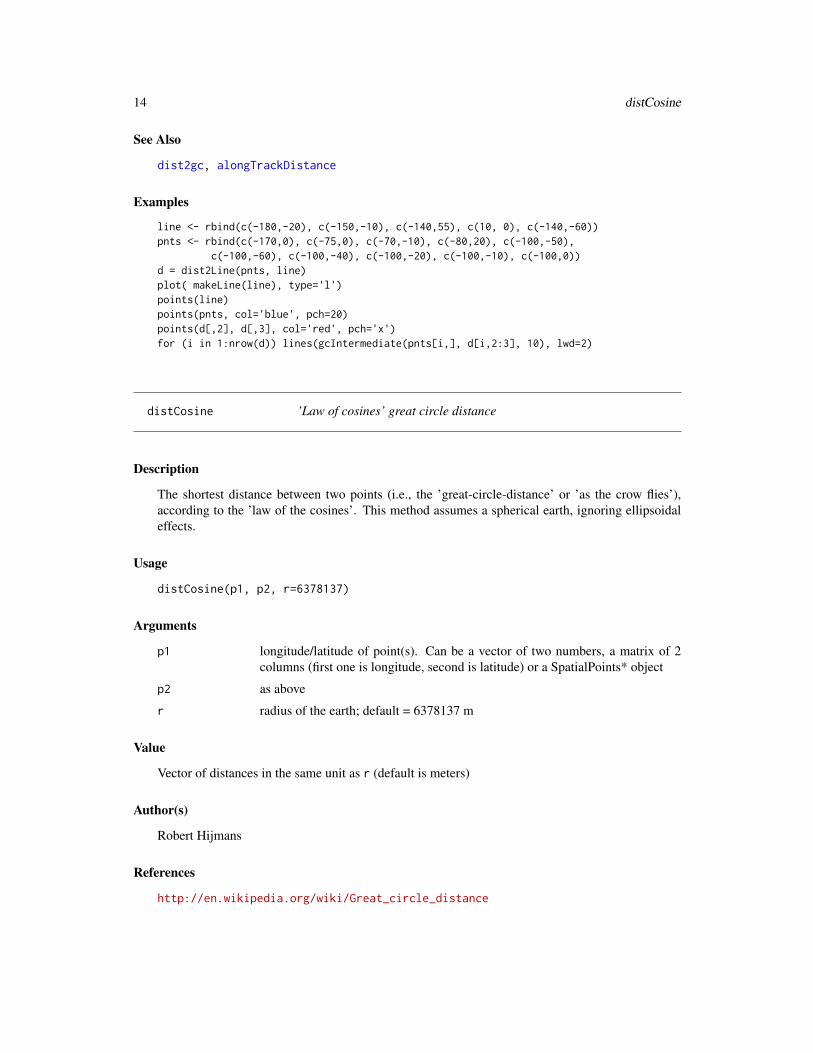
line <- rbind(c(-180,-20), c(-150,-10), c(-140,55), c(10, 0), c(-140,-60))pnts <- rbind(c(-170,0), c(-75,0), c(-70,-10), c(-80,20), c(-100,-50),
c(-100,-60), c(-100,-40), c(-100,-20), c(-100,-10), c(-100,0))d = dist2Line(pnts, line)plot( makeLine(line), type='l')points(line)points(pnts, col='blue', pch=20)points(d[,2], d[,3], col='red', pch='x')for (i in 1:nrow(d)) lines(gcIntermediate(pnts[i,], d[i,2:3], 10), lwd=2)
distCosine ’Law of cosines’ great circle distance
Description
The shortest distance between two points (i.e., the ’great-circle-distance’ or ’as the crow flies’),according to the ’law of the cosines’. This method assumes a spherical earth, ignoring ellipsoidaleffects.
Usage
distCosine(p1, p2, r=6378137)
Arguments
p1 longitude/latitude of point(s). Can be a vector of two numbers, a matrix of 2columns (first one is longitude, second is latitude) or a SpatialPoints* object
p2 as above
r radius of the earth; default = 6378137 m
Value
Vector of distances in the same unit as r (default is meters)
Author(s)
Robert Hijmans
References
http://en.wikipedia.org/wiki/Great_circle_distance

distGeo 15
See Also
distGeo, distHaversine, distVincentySphere, distVincentyEllipsoid, distMeeus
Examples
distCosine(c(0,0),c(90,90))
distGeo Distance on an ellipsoid (the geodesic)
Description
Highly accurate estimate of the shortest distance between two points on an ellipsoid (default isWGS84 ellipsoid). The shortest path between two points on an ellipsoid is called the geodesic.
Usage
distGeo(p1, p2, a=6378137, f=1/298.257223563)
Arguments
p1 longitude/latitude of point(s). Can be a vector of two numbers, a matrix of2 columns (first column is longitude, second column is latitude) or a Spatial-Points* object
p2 as above; or missing, in which case the sequential distance between the pointsin p1 is computed
a numeric. Major (equatorial) radius of the ellipsoid. The default value is forWGS84
f numeric. Ellipsoid flattening. The default value is for WGS84
Details
Parameters from the WGS84 ellipsoid are used by default. It is the best available global ellipsoid,but for some areas other ellipsoids could be preferable, or even necessary if you work with a printedmap that refers to that ellipsoid. Here are parameters for some commonly used ellipsoids. Also seethe refEllipsoids function.
ellipsoid a fWGS84 6378137 1/298.257223563GRS80 6378137 1/298.257222101GRS67 6378160 1/298.25Airy 1830 6377563.396 1/299.3249646Bessel 1841 6377397.155 1/299.1528434Clarke 1880 6378249.145 1/293.465Clarke 1866 6378206.4 1/294.9786982International 1924 6378388 1/297Krasovsky 1940 6378245 1/298.2997381

16 distHaversine
more info: http://en.wikipedia.org/wiki/Reference_ellipsoid
Value
Vector of distances in meters
Author(s)
This function calls GeographicLib code by C.F.F. Karney
References
C.F.F. Karney, 2013. Algorithms for geodesics, J. Geodesy 87: 43-55. https://dx.doi.org/10.1007/s00190-012-0578-z. Addenda: http://geographiclib.sf.net/geod-addenda.html.Also see http://geographiclib.sourceforge.net/
See Also
distCosine, distHaversine, distVincentySphere, distVincentyEllipsoid, distMeeus
Examples
distGeo(c(0,0),c(90,90))
distHaversine ’Haversine’ great circle distance
Description
The shortest distance between two points (i.e., the ’great-circle-distance’ or ’as the crow flies’),according to the ’haversine method’. This method assumes a spherical earth, ignoring ellipsoidaleffects.
Usage
distHaversine(p1, p2, r=6378137)
Arguments
p1 longitude/latitude of point(s). Can be a vector of two numbers, a matrix of 2columns (first one is longitude, second is latitude) or a SpatialPoints* object
p2 as above; or missing, in which case the sequential distance between the pointsin p1 is computed
r radius of the earth; default = 6378137 m

distm 17
Details
The Haversine (’half-versed-sine’) formula was published by R.W. Sinnott in 1984, although ithas been known for much longer. At that time computational precision was lower than today (15digits precision). With current precision, the spherical law of cosines formula appears to giveequally good results down to very small distances. If you want greater accuracy, you could usethe distVincentyEllipsoid method.
Value
Vector of distances in the same unit as r (default is meters)
Author(s)
Chris Veness and Robert Hijmans
References
Sinnott, R.W, 1984. Virtues of the Haversine. Sky and Telescope 68(2): 159
http://www.movable-type.co.uk/scripts/latlong.html
http://en.wikipedia.org/wiki/Great_circle_distance
See Also
distGeo, distCosine, distVincentySphere, distVincentyEllipsoid, distMeeus
Examples
distHaversine(c(0,0),c(90,90))
distm Distance matrix
Description
Distance matrix of a set of points, or between two sets of points
Usage
distm(x, y, fun=distGeo)
Arguments
x longitude/latitude of point(s). Can be a vector of two numbers, a matrix of 2columns (first one is longitude, second is latitude) or a SpatialPoints* object
y Same as x. If missing, y is the same as x
fun A function to compute distances (e.g., distCosine or distGeo)

18 distMeeus
Value
Matrix of distances
Author(s)
Robert Hijmans
References
http://en.wikipedia.org/wiki/Great_circle_distance
See Also
distGeo, distCosine, distHaversine, distVincentySphere, distVincentyEllipsoid
Examples
xy <- rbind(c(0,0),c(90,90),c(10,10),c(-120,-45))distm(xy)xy2 <- rbind(c(0,0),c(10,-10))distm(xy, xy2)
distMeeus ’Meeus’ great circle distance
Description
The shortest distance between two points on an ellipsoid (the ’geodetic’), according to the ’Meeus’method. distGeo should be more accurate.
Usage
distMeeus(p1, p2, a=6378137, f=1/298.257223563)
Arguments
p1 longitude/latitude of point(s), in degrees 1; can be a vector of two numbers, amatrix of 2 columns (first one is longitude, second is latitude) or a SpatialPoints*object
p2 as above; or missing, in which case the sequential distance between the pointsin p1 is computed
a numeric. Major (equatorial) radius of the ellipsoid. The default value is forWGS84
f numeric. Ellipsoid flattening. The default value is for WGS84

distMeeus 19
Details
Parameters from the WGS84 ellipsoid are used by default. It is the best available global ellipsoid,but for some areas other ellipsoids could be preferable, or even necessary if you work with a printedmap that refers to that ellipsoid. Here are parameters for some commonly used ellipsoids:
ellipsoid a fWGS84 6378137 1/298.257223563GRS80 6378137 1/298.257222101GRS67 6378160 1/298.25Airy 1830 6377563.396 1/299.3249646Bessel 1841 6377397.155 1/299.1528434Clarke 1880 6378249.145 1/293.465Clarke 1866 6378206.4 1/294.9786982International 1924 6378388 1/297Krasovsky 1940 6378245 1/298.2997381
more info: http://en.wikipedia.org/wiki/Reference_ellipsoid
Value
Distance value in the same units as parameter a of the ellipsoid (default is meters)
Note
This algorithm is also used in the spDists function in the sp package
Author(s)
Robert Hijmans, based on a script by Stephen R. Schmitt
References
Meeus, J., 1999 (2nd edition). Astronomical algoritms. Willman-Bell, 477p.
See Also
distGeo, distVincentyEllipsoid, distVincentySphere, distHaversine, distCosine
Examples
distMeeus(c(0,0),c(90,90))# on a 'Clarke 1880' ellipsoiddistMeeus(c(0,0),c(90,90), a=6378249.145, f=1/293.465)

20 distRhumb
distRhumb Distance along a rhumb line
Description
A rhumb line (loxodrome) is a path of constant bearing (direction), which crosses all meridians atthe same angle.
Usage
distRhumb(p1, p2, r=6378137)
Arguments
p1 longitude/latitude of point(s). Can be a vector of two numbers, a matrix of 2columns (first one is longitude, second is latitude) or a SpatialPoints* object
p2 as above; or missing, in which case the sequential distance between the pointsin p1 is computed
r radius of the earth; default = 6378137 m
Details
Rhumb (from the Spanish word for course, ’rumbo’) lines are straight lines on a Mercator projectionmap. They were used in navigation because it is easier to follow a constant compass bearing thanto continually adjust the bearing as is needed to follow a great circle, even though rhumb linesare normally longer than great-circle (orthodrome) routes. Most rhumb lines will gradually spiraltowards one of the poles.
Value
distance in units of r (default=meters)
Author(s)
Robert Hijmans and Chris Veness
References
http://www.movable-type.co.uk/scripts/latlong.html
See Also
distCosine, distHaversine, distVincentySphere, distVincentyEllipsoid
Examples
distRhumb(c(10,10),c(20,20))
distVincentyEllipsoid 21
distVincentyEllipsoid ’Vincenty’ (ellipsoid) great circle distance
Description
The shortest distance between two points (i.e., the ’great-circle-distance’ or ’as the crow flies’),according to the ’Vincenty (ellipsoid)’ method. This method uses an ellipsoid and the results arevery accurate. The method is computationally more intensive than the other great-circled methodsin this package.
Usage
distVincentyEllipsoid(p1, p2, a=6378137, b=6356752.3142, f=1/298.257223563)
Arguments
p1 longitude/latitude of point(s), in degrees 1; can be a vector of two numbers, amatrix of 2 columns (first one is longitude, second is latitude) or a SpatialPoints*object
p2 as above; or missing, in which case the sequential distance between the pointsin p1 is computed
a Equatorial axis of ellipsoid
b Polar axis of ellipsoid
f Inverse flattening of ellipsoid
Details
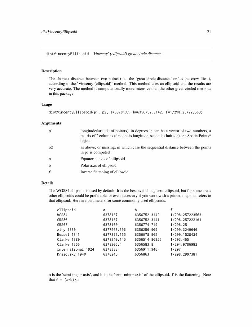
The WGS84 ellipsoid is used by default. It is the best available global ellipsoid, but for some areasother ellipsoids could be preferable, or even necessary if you work with a printed map that refers tothat ellipsoid. Here are parameters for some commonly used ellipsoids:
ellipsoid a b fWGS84 6378137 6356752.3142 1/298.257223563GRS80 6378137 6356752.3141 1/298.257222101GRS67 6378160 6356774.719 1/298.25Airy 1830 6377563.396 6356256.909 1/299.3249646Bessel 1841 6377397.155 6356078.965 1/299.1528434Clarke 1880 6378249.145 6356514.86955 1/293.465Clarke 1866 6378206.4 6356583.8 1/294.9786982International 1924 6378388 6356911.946 1/297Krasovsky 1940 6378245 6356863 1/298.2997381
a is the ’semi-major axis’, and b is the ’semi-minor axis’ of the ellipsoid. f is the flattening. Notethat f = (a-b)/a

22 distVincentySphere
more info: http://en.wikipedia.org/wiki/Reference_ellipsoid
Value
Distance value in the same units as the ellipsoid (default is meters)
Author(s)
Chris Veness and Robert Hijmans
References
Vincenty, T. 1975. Direct and inverse solutions of geodesics on the ellipsoid with application ofnested equations. Survey Review Vol. 23, No. 176, pp88-93. Available here:
http://www.movable-type.co.uk/scripts/latlong-vincenty.html
http://en.wikipedia.org/wiki/Great_circle_distance
See Also
distGeo, distVincentySphere, distHaversine, distCosine, distMeeus
Examples
distVincentyEllipsoid(c(0,0),c(90,90))# on a 'Clarke 1880' ellipsoiddistVincentyEllipsoid(c(0,0),c(90,90), a=6378249.145, b=6356514.86955, f=1/293.465)
distVincentySphere ’Vincenty’ (sphere) great circle distance
Description
The shortest distance between two points (i.e., the ’great-circle-distance’ or ’as the crow flies’),according to the ’Vincenty (sphere)’ method. This method assumes a spherical earth, ignoringellipsoidal effects and it is less accurate then the distVicentyEllipsoid method.
Usage
distVincentySphere(p1, p2, r=6378137)
Arguments
p1 longitude/latitude of point(s). Can be a vector of two numbers, a matrix of 2columns (first one is longitude, second is latitude) or a SpatialPoints* object
p2 as above; or missing, in which case the sequential distance between the pointsin p1 is computed
r radius of the earth; default = 6378137 m

finalBearing 23
Value
Distance value in the same unit as r (default is meters)
Author(s)
Robert Hijmans
References
http://en.wikipedia.org/wiki/Great_circle_distance
See Also
distGeo, distVincentyEllipsoid, distHaversine, distCosine, distMeeus
Examples
distVincentySphere(c(0,0),c(90,90))
finalBearing Final direction
Description
Get the final direction (bearing) when arriving at p2 after starting from p1 and following the shortestpath on an ellipsoid (following a geodetic) or on a sphere (following a great circle).
Usage
finalBearing(p1, p2, a=6378137, f=1/298.257223563, sphere=FALSE)
Arguments
p1 longitude/latitude of point(s). Can be a vector of two numbers, a matrix of2 columns (first column is longitude, second column is latitude) or a Spatial-Points* object
p2 as above
a major (equatorial) radius of the ellipsoid. The default value is for WGS84
f ellipsoid flattening. The default value is for WGS84
sphere logical. If TRUE, the bearing is computed for a sphere, instead of for an ellipsoid
Value
A vector of directions (bearings) in degrees

24 gcIntersect
Author(s)
This function calls GeographicLib code by C.F.F. Karney
References
C.F.F. Karney, 2013. Algorithms for geodesics, J. Geodesy 87: 43-55. https://dx.doi.org/10.1007/s00190-012-0578-z. Addenda: http://geographiclib.sf.net/geod-addenda.html.Also see http://geographiclib.sourceforge.net/
See Also
bearing
Examples
bearing(c(10,10),c(20,20))finalBearing(c(10,10),c(20,20))
gcIntersect Intersections of two great circles
Description
Get the two points where two great cricles cross each other. Great circles are defined by two pointson it.
Usage
gcIntersect(p1, p2, p3, p4)
Arguments
p1 Longitude/latitude of a single point, in degrees; can be a vector of two numbers,a matrix of 2 columns (first one is longitude, second is latitude) or a Spatial-Points* object
p2 As above
p3 As above
p4 As above
Value
two points for each pair of great circles
Author(s)
Robert Hijmans, based on equations by Ed Williams (see reference)

gcIntersectBearing 25
References
http://www.edwilliams.org/intersect.htm
See Also
gcIntersectBearing
Examples
p1 <- c(5,52); p2 <- c(-120,37); p3 <- c(-60,0); p4 <- c(0,70)gcIntersect(p1,p2,p3,p4)
gcIntersectBearing Intersections of two great circles
Description
Get the two points where two great cricles cross each other. In this function, great circles are definedby a points and an initial bearing. In function gcIntersect they are defined by two sets of points.
Usage
gcIntersectBearing(p1, brng1, p2, brng2)
Arguments
p1 longitude/latitude of point(s). Can be a vector of two numbers, a matrix of 2columns (first one is longitude, second is latitude) or a SpatialPoints* object
brng1 Bearing from p1
p2 As above. Should have same length as p1, or a single point (or vice versa whenp1 is a single point
brng2 Bearing from p2
Value
a matrix with four columns (two points)
Author(s)
Chris Veness and Robert Hijmans based on code by Ed Williams
References
http://www.edwilliams.org/avform.htm#Intersection
http://www.movable-type.co.uk/scripts/latlong.html

26 gcLat
See Also
gcIntersect
Examples
gcIntersectBearing(c(10,0), 10, c(-10,0), 10)
gcLat Latitude on a Great Circle
Description
Latitude at which a great circle crosses a longitude
Usage
gcLat(p1, p2, lon)
Arguments
p1 Longitude/latitude of a single point, in degrees; can be a vector of two numbers,a matrix of 2 columns (first one is longitude, second is latitude) or a Spatial-Points* object
p2 As above
lon Longitude
Value
A numeric (latitude)
Author(s)
Robert Hijmans based on a formula by Ed Williams
References
http://www.edwilliams.org/avform.htm#Int
See Also
gcLon, gcMaxLat
Examples
gcLat(c(5,52), c(-120,37), lon=-120)

gcLon 27
gcLon Longitude on a Great Circle
Description
Longitudes at which a great circle crosses a latitude (parallel)
Usage
gcLon(p1, p2, lat)
Arguments
p1 longitude/latitude of point(s). Can be a vector of two numbers, a matrix of 2columns (first one is longitude, second is latitude) or a SpatialPoints* object
p2 as above
lat a latitude
Value
vector of two numbers (longitudes)
Author(s)
Robert Hijmans based on code by Ed Williams
References
http://www.edwilliams.org/avform.htm#Intersection
See Also
gcLat, gcMaxLat
Examples
gcLon(c(5,52), c(-120,37), 40)

28 gcMaxLat
gcMaxLat Highest latitude on a great circle
Description
What is northern most point that will be reached when following a great circle? Computed withClairaut’s formula. The southern most point is the antipode of the northern-most point. This doesnot seem to be very precise; and you could use optimization instead to find this point (see examples)
Usage
gcMaxLat(p1, p2)
Arguments
p1 longitude/latitude of point(s). Can be a vector of two numbers, a matrix of 2columns (first one is longitude, second is latitude) or a SpatialPoints* object
p2 as above
Value
A matrix with coordinates (longitude/latitude)
Author(s)
Ed Williams, Chris Veness, Robert Hijmans
References
http://www.edwilliams.org/ftp/avsig/avform.txt
http://www.movable-type.co.uk/scripts/latlong.html
See Also
gcLat, gcLon
Examples
gcMaxLat(c(5,52), c(-120,37))
# Another way to get there:f <- function(lon){gcLat(c(5,52), c(-120,37), lon)}optimize(f, interval=c(-180, 180), maximum=TRUE)

geodesic 29
geodesic geodesic and inverse geodesic problem
Description
Highly accurate estimate of the ’geodesic problem’ (find location and azimuth at arrival when de-parting from a location, given an direction (azimuth) at departure and distance) and the ’inversegeodesic problem’ (find the distance between two points and the azimuth of departure and arrivalfor the shortest path. Computations are for an ellipsoid (default is WGS84 ellipsoid).
This is a direct implementation of the the GeographicLib code by C.F.F. Karney that is also used inseveral other functions in this package (for example, in distGeo and areaPolygon).
Usage
geodesic(p, azi, d, a=6378137, f=1/298.257223563, ...)
geodesic_inverse(p1, p2, a=6378137, f=1/298.257223563, ...)
Arguments
p longitude/latitude of point(s). Can be a vector of two numbers, a matrix of2 columns (first column is longitude, second column is latitude) or a Spatial-Points* object
p1 as above
p2 as above
azi numeric. Azimuth of departure in degrees
d numeric. Distance in meters
a numeric. Major (equatorial) radius of the ellipsoid. The default value is forWGS84
f numeric. Ellipsoid flattening. The default value is for WGS84
... additional arguments (none implemented)
Details
Parameters from the WGS84 ellipsoid are used by default. It is the best available global ellipsoid,but for some areas other ellipsoids could be preferable, or even necessary if you work with a printedmap that refers to that ellipsoid. Here are parameters for some commonly used ellipsoids.
ellipsoid a fWGS84 6378137 1/298.257223563GRS80 6378137 1/298.257222101GRS67 6378160 1/298.25Airy 1830 6377563.396 1/299.3249646Bessel 1841 6377397.155 1/299.1528434Clarke 1880 6378249.145 1/293.465

30 geomean
Clarke 1866 6378206.4 1/294.9786982International 1924 6378388 1/297Krasovsky 1940 6378245 1/298.2997381
more info: http://en.wikipedia.org/wiki/Reference_ellipsoid
Value
Three column matrix with columns ’longitude’, ’latitude’, ’azimuth’ (geodesic); or ’distance’ (inmeters), ’azimuth1’ (of departure), ’azimuth2’ (of arrival) (geodesic_inverse)
Author(s)
This function calls GeographicLib code by C.F.F. Karney
References
C.F.F. Karney, 2013. Algorithms for geodesics, J. Geodesy 87: 43-55. https://dx.doi.org/10.1007/s00190-012-0578-z. Addenda: http://geographiclib.sf.net/geod-addenda.html.Also see http://geographiclib.sourceforge.net/
See Also
distGeo
Examples
geodesic(cbind(0,0), 30, 1000000)geodesic_inverse(cbind(0,0), cbind(90,90))
geomean Mean location of sperhical coordinates
Description
mean location for spherical (longitude/latitude) coordinates that deals with the angularity. I.e., themean of longitudes -179 and 178 is 179.5
Usage
geomean(xy, w)
Arguments
xy matrix with two columns (longitude/latitude), or a SpatialPoints or SpatialPoly-gons object with a longitude/latitude CRS
w weights (vector of numeric values, with a length that is equal to the number ofspatial features in x

greatCircle 31
Value
Ccoordinate pair (numeric)
Author(s)
Robert J. Hijmans
Examples
xy <- cbind(x=c(-179,179, 177), y=c(12,14,16))xygeomean(xy)
greatCircle Great circle
Description
Get points on a great circle as defined by the shortest distance between two specified points
Usage
greatCircle(p1, p2, n=360, sp=FALSE)
Arguments
p1 longitude/latitude of point(s). Can be a vector of two numbers, a matrix of 2columns (first one is longitude, second is latitude) or a SpatialPoints* object
p2 as above
n The requested number of points on the Great Circle
sp Logical. Return a SpatialLines object?
Value
A matrix of points, or a list of such matrices (e.g., if multiple bearings are supplied)
Author(s)
Robert Hijmans, based on a formula provided by Ed Williams
References
http://www.edwilliams.org/avform.htm#Int
Examples
greatCircle(c(5,52), c(-120,37), n=36)

32 horizon
greatCircleBearing Great circle
Description
Get points on a great circle as defined by a point and an initial bearing
Usage
greatCircleBearing(p, brng, n=360)
Arguments
p longitude/latitude of a single point. Can be a vector of two numbers, a matrix of2 columns (first one is longitude, second is latitude) or a SpatialPoints* object
brng bearing
n The requested number of points on the great circle
Value
A matrix of points, or a list of matrices (e.g., if multiple bearings are supplied)
Author(s)
Robert Hijmans based on formulae by Ed Williams
References
http://www.edwilliams.org/avform.htm#Int
Examples
greatCircleBearing(c(5,52), 45, n=12)
horizon Distance to the horizon
Description
Empirical function to compute the distance to the horizon from a given altitude. The earth is as-sumed to be smooth, i.e. mountains and other obstacles are ignored.
Usage
horizon(h, r=6378137)

intermediate 33
Arguments
h altitude, numeric >= 0. Should have the same unit as rr radius of the earth; default value is 6378137 m
Value
Distance in units of h (default is meters)
Author(s)
Robert J. Hijmans
References
http://www.edwilliams.org/avform.htm#Horizon
Bowditch, 1995. American Practical Navigator. Table 12.
Examples
horizon(1.80) # mehorizon(324) # Eiffel tower
intermediate Intermediate points on a great circle (sphere)
Description
Get intermediate points (way points) between the two locations with longitude/latitude coordinates.gcIntermediate is based on a spherical model of the earth and internally uses distCosine.
Usage
gcIntermediate(p1, p2, n=50, breakAtDateLine=FALSE, addStartEnd=FALSE, sp=FALSE, sepNA)
Arguments
p1 longitude/latitude of a single point, in degrees. This can be a vector of twonumbers, a matrix of 2 columns (first one is longitude, second is latitude) or aSpatialPoints* object
p2 as for p1n integer. The desired number of intermediate pointsbreakAtDateLine
logical. Return two matrices if the dateline is crossed?addStartEnd logical. Add p1 and p2 to the result?sp logical. Return a SpatialLines object?sepNA logical. Rather than as a list, return the values as a two column matrix with lines
seperated by a row of NA values? (for use in ’plot’)

34 lengthLine
Value
matrix or list with intermediate points
Author(s)
Robert Hijmans based on code by Ed Williams (great circle)
References
http://www.edwilliams.org/avform.htm#Intermediate
Examples
gcIntermediate(c(5,52), c(-120,37), n=6, addStartEnd=TRUE)
lengthLine Length of lines
Description
Compute the length of lines
Usage
lengthLine(line)
Arguments
line longitude/latitude of line as a matrix of 2 columns (first one is longitude, secondis latitude) or a SpatialLines* or SpatialPolygons* object
Value
length (in meters) for each line
See Also
For planar coordinates, see gLength
Examples
line <- rbind(c(-180,-20), c(-150,-10), c(-140,55), c(10, 0), c(-140,-60))d <- lengthLine(line)

makePoly 35
makePoly Add vertices to a polygon or line
Description
Make a polygon or line by adding intermedate points (vertices) on the great circles inbetween thepoints supplied. This can be relevant when vertices are relatively far apart. It can make the shape ofthe object to be accurate, when plotted on a plane. makePoly will also close the polygon if needed.
Usage
makePoly(p, interval=10000, sp=FALSE, ...)makeLine(p, interval=10000, sp=FALSE, ...)
Arguments
p a 2-column matrix (longitude/latitude) or a SpatialPolygons or SpatialLines ob-ject
interval maximum interval of points, in units of r
sp Logical. If TRUE, a SpatialPolygons object is retunred (depends on the ’sp’ pack-age)
... additional arguments passed to distGeo
Value
A matrix
Author(s)
Robert J. Hijmans
Examples
pol <- rbind(c(-180,-20), c(-160,5), c(-60, 0), c(-160,-60), c(-180,-20))plot(pol)lines(pol, col='red', lwd=3)pol2 = makePoly(pol, interval=100000)lines(pol2, col='blue', lwd=2)

36 midPoint
mercator Mercator projection
Description
Transform longitude/latiude points to the Mercator projection. The main purpose of this function isto compute centroids, and to illustrate rhumb lines in the vignette.
Usage
mercator(p, inverse=FALSE, r=6378137)
Arguments
p longitude/latitude of point(s). Can be a vector of two numbers, a matrix of 2columns (first one is longitude, second is latitude) or a SpatialPoints* object
inverse Logical. If TRUE, do the inverse projection (from Mercator to longitude/latitude
r Numeric. Radius of the earth; default = 6378137 m
Value
matrix
Author(s)
Robert Hijmans
Examples
a = mercator(c(5,52))amercator(a, inverse=TRUE)
midPoint Mid-point
Description
Find the point half-way between two points along an ellipsoid
Usage
midPoint(p1, p2, a=6378137, f = 1/298.257223563)

onGreatCircle 37
Arguments
p1 longitude/latitude of point(s). Can be a vector of two numbers, a matrix of 2columns (first one is longitude, second is latitude) or a SpatialPoints* object
p2 As above
a major (equatorial) radius of the ellipsoid
f ellipsoid flattening. The default value is for WGS84
Value
matrix with coordinate pairs
Author(s)
Elias Pipping and Robert Hijmans
Examples
midPoint(c(0,0),c(90,90))midPoint(c(0,0),c(90,90), f=0)
onGreatCircle Is a point on a given great circle?
Description
Test if a point is on a great circle defined by two other points.
Usage
onGreatCircle(p1, p2, p3, tol=0.0001)
Arguments
p1 Longitude/latitude of the first point defining a great circle, in degrees; can be avector of two numbers, a matrix of 2 columns (first one is longitude, second islatitude) or a SpatialPoints* object
p2 as above for the second point
p3 the point(s) to be tested if they are on the great circle or not
tol numeric. maximum distance from the great circle (in degrees) that is toleratedto be considered on the circle
Value
logical

38 perimeter
Author(s)
Robert Hijmans
Examples
onGreatCircle(c(0,0), c(30,30), rbind(c(-10 -11.33812), c(10,20)))
perimeter Compute the perimeter of a longitude/latitude polygon
Description
Compute the perimeter of a polygon (or the length of a line) with longitude/latitude coordinates, onan ellipsoid (WGS84 by default)
Usage
## S4 method for signature 'matrix'perimeter(x, a=6378137, f=1/298.257223563, ...)
## S4 method for signature 'SpatialPolygons'perimeter(x, a=6378137, f=1/298.257223563, ...)
## S4 method for signature 'SpatialLines'perimeter(x, a=6378137, f=1/298.257223563, ...)
Arguments
x Longitude/latitude of the points forming a polygon or line; Must be a matrix of2 columns (first one is longitude, second is latitude) or a SpatialPolygons* orSpatialLines* object
a major (equatorial) radius of the ellipsoid. The default value is for WGS84f ellipsoid flattening. The default value is for WGS84... Additional arguments. None implemented
Value
Numeric. The perimeter or length in m.
Author(s)
This function calls GeographicLib code by C.F.F. Karney
References
C.F.F. Karney, 2013. Algorithms for geodesics, J. Geodesy 87: 43-55. https://dx.doi.org/10.1007/s00190-012-0578-z. Addenda: http://geographiclib.sf.net/geod-addenda.html.Also see http://geographiclib.sourceforge.net/

plotArrows 39
See Also
areaPolygon, centroid
Examples
xy <- rbind(c(-180,-20), c(-140,55), c(10, 0), c(-140,-60), c(-180,-20))perimeter(xy)
plotArrows Plot
Description
Plot polygons with arrow heads on each line segment, pointing towards the next vertex. This showsthe direction of each line segment.
Usage
plotArrows(p, fraction=0.9, length=0.15, first='', add=FALSE, ...)
Arguments
p Polygons (either a 2 column matrix or data.frame; or a SpatialPolygons* object
fraction numeric between 0 and 1. When smaller then 1, interrupted lines are drawn
length length of the edges of the arrow head (in inches)
first Character to plot on first (and last) vertex
add Logical. If TRUE, the plot is added to an existing plot
... Additional arguments, see Details
Note
Based on an example in Software for Data Analysis by John Chambers (pp 250-251) but adjustedsuch that the line segments follow great circles between vertices.
Author(s)
Robert J. Hijmans
Examples
pol <- rbind(c(-180,-20), c(-160,5), c(-60, 0), c(-160,-60), c(-180,-20))plotArrows(pol)

40 randomCoordinates
randomCoordinates Random or regularly distributed coordinates on the globe
Description
randomCoordinates returns a ’uniform random sample’ in the sense that the probability that a pointis drawn from any region is equal to the area of that region divided by the area of the entire sphere.This would not happen if you took a random uniform sample of longitude and latitude, as the samplewould be biased towards the poles.
regularCoordiaates returns a set of coordinates that are regularly distributed on the globe.
Usage
randomCoordinates(n)regularCoordinates(N)
Arguments
n Sample size (number of points (coordinate pairs))
N Number of ’parts’ in which the earth is subdived )
Value
Matrix of lon/lat coordiantes
Author(s)
Robert Hijmans, based on code by Nils Haeck (regularCoordinates), http://mathforum.org/kb/message.jspa?messageID=3985660&tstart=0
and suggstions by Michael Orion (randomCoordinates), http://sci.tech-archive.net/Archive/sci.math/2005-09/msg04691.html
Examples
randomCoordinates(3)regularCoordinates(1)

refEllipsoids 41
refEllipsoids Reference ellipsoids
Description
This function returns a data.frame with parameters a (semi-major axis) and 1/f (inverse flattening)for a set of reference ellipsoids.
Usage
refEllipsoids()
Value
data.frame
Note
To compute parameter b you can do
Author(s)
Robert J. Hijmans
See Also
area, perimeter
Examples
e <- refEllipsoids()e[e$code=='WE', ]
#to compute semi-minor axis b:e$b <- e$a - e$a / e$invf
span Span of polygons
Description
Compute the approximate surface span of polygons in longitude and latitude direction. Span iscomputed by rasterizing the polygons; and precision increases with the number of ’scan lines’. Youcan either use a fixed number of scan lines for each polygon, or a fixed band-width.

42 wrld
Usage
span(x, ...)
Arguments
x a SpatialPolygons* object or a 2-column matrix (longitude/latitude)
... Additional arguments, see Details
Details
The following additional arguments can be passed, to replace default values for this function
nbands Character. Method to determine the number of bands to ’scan’ the polygon. Either ’fixed’ or ’variable’n Integer >= 1. If nbands=’fixed’, how many bands should be usedres Numeric. If nbands=’variable’, what should the bandwidth be (in degrees)?fun Logical. A function such as mean or min. Mean computes the average span... further additional arguments passed to distGeo
Value
A list, or a matrix if a function fun is specified. Values are in the units of r (default is meter)
Author(s)
Robert J. Hijmans
Examples
pol <- rbind(c(-180,-20), c(-160,5), c(-60, 0), c(-160,-60), c(-180,-20))plot(pol)lines(pol)# lon and lat span in mspan(pol, fun=max)x <- span(pol)max(x$latspan)mean(x$latspan)plot(x$longitude, x$lonspan)
wrld World countries
Description
world coastline and country outlines in longitude/latitude (wrld) and in Mercator projection (merc).

wrld 43
Usage
data(wrld)data(merc)
Source
Derived from the wrld_simpl data set in package maptools

Index
∗Topic datasetswrld, 42
∗Topic methodscentroid, 8geomean, 30makePoly, 35plotArrows, 39refEllipsoids, 41span, 41
∗Topic packagegeosphere-package, 2
∗Topic spatialalongTrackDistance, 3antipode, 4areaPolygon, 5bearing, 6bearingRhumb, 7centroid, 8daylength, 9destPoint, 10destPointRhumb, 11dist2gc, 12dist2Line, 13distCosine, 14distGeo, 15distHaversine, 16distm, 17distMeeus, 18distRhumb, 20distVincentyEllipsoid, 21distVincentySphere, 22finalBearing, 23gcIntersect, 24gcIntersectBearing, 25gcLat, 26gcLon, 27gcMaxLat, 28geodesic, 29geomean, 30
geosphere-package, 2greatCircle, 31greatCircleBearing, 32horizon, 32intermediate, 33lengthLine, 34makePoly, 35mercator, 36midPoint, 36onGreatCircle, 37perimeter, 38plotArrows, 39randomCoordinates, 40refEllipsoids, 41span, 41
alongTrackDistance, 3, 13, 14antipodal (antipode), 4antipode, 4, 28area, 9, 41areaPolygon, 5, 29, 39areaPolygon,data.frame-method
(areaPolygon), 5areaPolygon,matrix-method
(areaPolygon), 5areaPolygon,SpatialPolygons-method
(areaPolygon), 5
bearing, 6, 8, 24bearingRhumb, 6, 7, 7
centroid, 6, 8, 39centroid,data.frame-method (centroid), 8centroid,matrix-method (centroid), 8centroid,SpatialPolygons-method
(centroid), 8
daylength, 9destPoint, 10, 12destPointRhumb, 11
44

INDEX 45
dist2gc, 3, 4, 12, 14dist2Line, 13, 13distCosine, 14, 16–20, 22, 23, 33distGeo, 13, 15, 15, 17–19, 22, 23, 29, 30distHaversine, 15, 16, 16, 18–20, 22, 23distm, 17distMeeus, 15–17, 18, 22, 23distRhumb, 8, 20distVincentyEllipsoid, 15–20, 21, 23distVincentySphere, 15–20, 22, 22
finalBearing, 11, 23
gcIntermediate (intermediate), 33gcIntersect, 24, 25, 26gcIntersectBearing, 25, 25gcLat, 26, 27, 28gcLon, 26, 27, 28gcMaxLat, 26, 27, 28geodesic, 29geodesic_inverse (geodesic), 29geomean, 30geosphere (geosphere-package), 2geosphere-package, 2gLength, 34greatCircle, 31greatCircleBearing, 32
horizon, 32
intermediate, 33
lengthLine, 34
makeLine (makePoly), 35makePoly, 35merc (wrld), 42mercator, 36midPoint, 36
onGreatCircle, 37
perimeter, 6, 9, 38, 41perimeter,data.frame-method
(perimeter), 38perimeter,matrix-method (perimeter), 38perimeter,SpatialLines-method
(perimeter), 38perimeter,SpatialPolygons-method
(perimeter), 38
plotArrows, 39
randomCoordinates, 40refEllipsoids, 15, 41regularCoordinates (randomCoordinates),
40
span, 41span,matrix-method (span), 41span,SpatialPolygons-method (span), 41
wrld, 42