Package ‘ﬂexclust’ - The Comprehensive R Archive Network · · 2018-02-15Package ‘ﬂexclust’ February 15, 2018 Version 1.3-5 Date 2018-02-14 Title Flexible Cluster Algorithms

Package ‘flexclust’February 15, 2018

Version 1.3-5

Date 2018-02-14

Title Flexible Cluster Algorithms

Depends R (>= 2.14.0), graphics, grid, lattice, modeltools

Imports methods, parallel, stats, stats4

Suggests ellipse, clue, cluster, seriation

Description The main function kcca implements a general framework fork-centroids cluster analysis supporting arbitrary distancemeasures and centroid computation. Further cluster methodsinclude hard competitive learning, neural gas, and QTclustering. There are numerous visualization methods forcluster results (neighborhood graphs, convex cluster hulls,barcharts of centroids, ...), and bootstrap methods for theanalysis of cluster stability.

License GPL-2

Encoding UTF-8

Author Friedrich Leisch [aut, cre],Evgenia Dimitriadou [ctb]

Maintainer ORPHANED

NeedsCompilation yes

X-CRAN-Comment Orphaned and corrected on 2018-02-14 as check errorswere not corrected despite reminders.Included incorrect formula for Canberra distance, no registration,missing imports.

Repository CRAN

Date/Publication 2018-02-14 14:38:52

X-CRAN-Original-Maintainer Friedrich Leisch<[email protected]>

1

2 R topics documented:

R topics documented:

achieve . . . . . . . . . . . . . . . . . . . . . . . . . . . . . . . . . . . . . . . . . . . 3auto . . . . . . . . . . . . . . . . . . . . . . . . . . . . . . . . . . . . . . . . . . . . . 3barplot-methods . . . . . . . . . . . . . . . . . . . . . . . . . . . . . . . . . . . . . . . 5birth . . . . . . . . . . . . . . . . . . . . . . . . . . . . . . . . . . . . . . . . . . . . . 7bootFlexclust . . . . . . . . . . . . . . . . . . . . . . . . . . . . . . . . . . . . . . . . 8bundestag . . . . . . . . . . . . . . . . . . . . . . . . . . . . . . . . . . . . . . . . . . 9bwplot-methods . . . . . . . . . . . . . . . . . . . . . . . . . . . . . . . . . . . . . . . 11cclust . . . . . . . . . . . . . . . . . . . . . . . . . . . . . . . . . . . . . . . . . . . . 12clusterSim . . . . . . . . . . . . . . . . . . . . . . . . . . . . . . . . . . . . . . . . . . 14conversion . . . . . . . . . . . . . . . . . . . . . . . . . . . . . . . . . . . . . . . . . . 16dentitio . . . . . . . . . . . . . . . . . . . . . . . . . . . . . . . . . . . . . . . . . . . 17dist2 . . . . . . . . . . . . . . . . . . . . . . . . . . . . . . . . . . . . . . . . . . . . . 18distances . . . . . . . . . . . . . . . . . . . . . . . . . . . . . . . . . . . . . . . . . . . 19flexclustControl-class . . . . . . . . . . . . . . . . . . . . . . . . . . . . . . . . . . . . 20flxColors . . . . . . . . . . . . . . . . . . . . . . . . . . . . . . . . . . . . . . . . . . 22image-methods . . . . . . . . . . . . . . . . . . . . . . . . . . . . . . . . . . . . . . . 23info . . . . . . . . . . . . . . . . . . . . . . . . . . . . . . . . . . . . . . . . . . . . . 24kcca . . . . . . . . . . . . . . . . . . . . . . . . . . . . . . . . . . . . . . . . . . . . . 25kcca2df . . . . . . . . . . . . . . . . . . . . . . . . . . . . . . . . . . . . . . . . . . . 28milk . . . . . . . . . . . . . . . . . . . . . . . . . . . . . . . . . . . . . . . . . . . . . 28Nclus . . . . . . . . . . . . . . . . . . . . . . . . . . . . . . . . . . . . . . . . . . . . 29nutrient . . . . . . . . . . . . . . . . . . . . . . . . . . . . . . . . . . . . . . . . . . . 30pairs-methods . . . . . . . . . . . . . . . . . . . . . . . . . . . . . . . . . . . . . . . . 30parameters . . . . . . . . . . . . . . . . . . . . . . . . . . . . . . . . . . . . . . . . . . 31plot-methods . . . . . . . . . . . . . . . . . . . . . . . . . . . . . . . . . . . . . . . . 31predict-methods . . . . . . . . . . . . . . . . . . . . . . . . . . . . . . . . . . . . . . . 33priceFeature . . . . . . . . . . . . . . . . . . . . . . . . . . . . . . . . . . . . . . . . . 33projAxes . . . . . . . . . . . . . . . . . . . . . . . . . . . . . . . . . . . . . . . . . . . 34propBarchart . . . . . . . . . . . . . . . . . . . . . . . . . . . . . . . . . . . . . . . . 36qtclust . . . . . . . . . . . . . . . . . . . . . . . . . . . . . . . . . . . . . . . . . . . . 38randIndex . . . . . . . . . . . . . . . . . . . . . . . . . . . . . . . . . . . . . . . . . . 39randomTour . . . . . . . . . . . . . . . . . . . . . . . . . . . . . . . . . . . . . . . . . 41shadow . . . . . . . . . . . . . . . . . . . . . . . . . . . . . . . . . . . . . . . . . . . 43shadowStars . . . . . . . . . . . . . . . . . . . . . . . . . . . . . . . . . . . . . . . . . 44stepFlexclust . . . . . . . . . . . . . . . . . . . . . . . . . . . . . . . . . . . . . . . . 46stripes . . . . . . . . . . . . . . . . . . . . . . . . . . . . . . . . . . . . . . . . . . . . 48volunteers . . . . . . . . . . . . . . . . . . . . . . . . . . . . . . . . . . . . . . . . . . 49

Index 51

achieve 3

achieve Achievement Test Scores for New Haven Schools

Description

Measurements at the beginning of the 4th grade (when the national average is 4.0) and of the 6thgrade in 25 schools in New Haven.

Usage

data(achieve)

Format

A data frame with 25 observations on the following 4 variables.

read4: 4th grade reading

arith4: 4th grade arithmetic

read6: 6th grade reading

arith6: 6th grade arithmetic

References

John A. Hartigan: Clustering Algorithms. Wiley, New York, 1975.

auto Automobile Customer Survey Data

Description

A German manufacturer of premium cars asked customers approximately 3 months after a carpurchase which characteristics of the car were most important for the decision to buy the car. Thesurvey was done in 1983 and the data set contains all responses without missing values.

Usage

data(auto)

4 auto

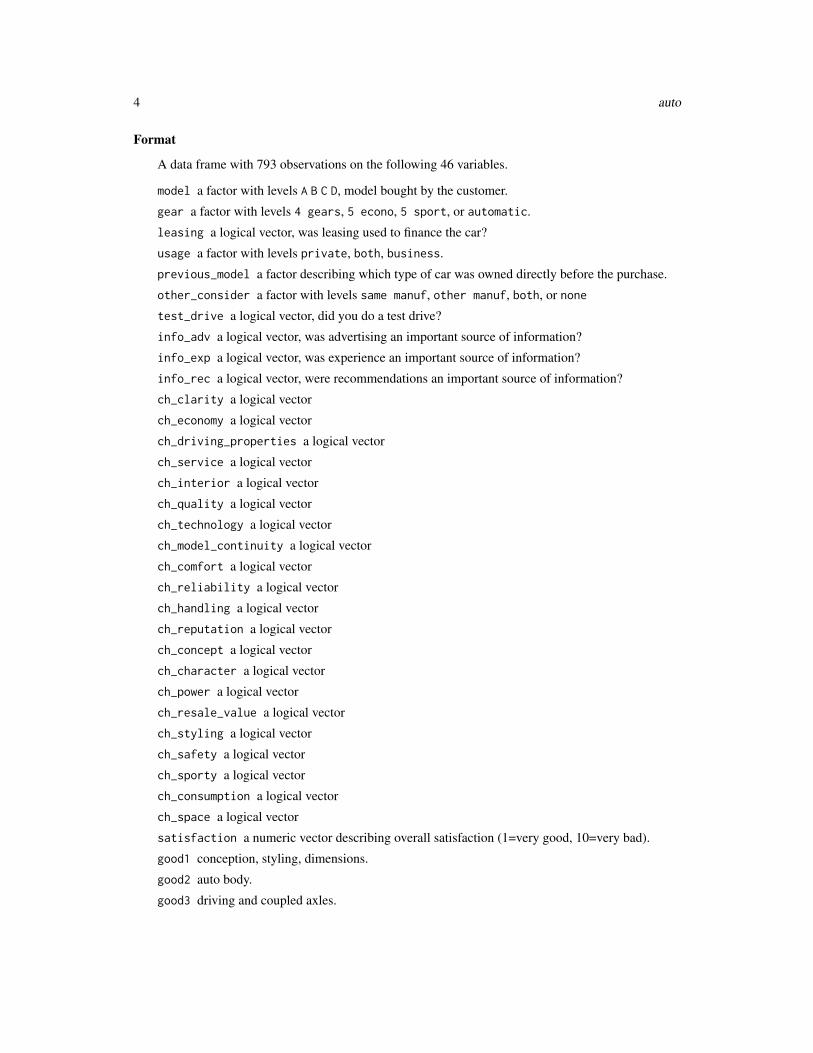
Format


model a factor with levels A B C D, model bought by the customer.

gear a factor with levels 4 gears, 5 econo, 5 sport, or automatic.

leasing a logical vector, was leasing used to finance the car?

usage a factor with levels private, both, business.

previous_model a factor describing which type of car was owned directly before the purchase.

other_consider a factor with levels same manuf, other manuf, both, or none

test_drive a logical vector, did you do a test drive?

info_adv a logical vector, was advertising an important source of information?

info_exp a logical vector, was experience an important source of information?

info_rec a logical vector, were recommendations an important source of information?

ch_clarity a logical vector

ch_economy a logical vector

ch_driving_properties a logical vector

ch_service a logical vector

ch_interior a logical vector

ch_quality a logical vector

ch_technology a logical vector

ch_model_continuity a logical vector

ch_comfort a logical vector

ch_reliability a logical vector

ch_handling a logical vector

ch_reputation a logical vector

ch_concept a logical vector

ch_character a logical vector

ch_power a logical vector

ch_resale_value a logical vector

ch_styling a logical vector

ch_safety a logical vector

ch_sporty a logical vector

ch_consumption a logical vector

ch_space a logical vector

satisfaction a numeric vector describing overall satisfaction (1=very good, 10=very bad).

good1 conception, styling, dimensions.

good2 auto body.

good3 driving and coupled axles.

barplot-methods 5

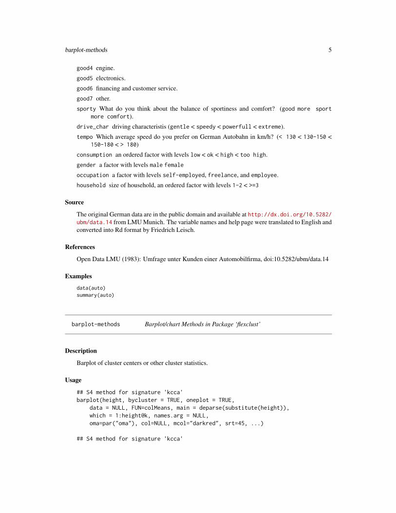
good4 engine.

good5 electronics.

good6 financing and customer service.

good7 other.

sporty What do you think about the balance of sportiness and comfort? (good more sportmore comfort).

drive_char driving characteristis (gentle < speedy < powerfull < extreme).

tempo Which average speed do you prefer on German Autobahn in km/h? (< 130 < 130-150 <150-180 < > 180)

consumption an ordered factor with levels low < ok < high < too high.

gender a factor with levels male female

occupation a factor with levels self-employed, freelance, and employee.

household size of household, an ordered factor with levels 1-2 < >=3

Source

The original German data are in the public domain and available at http://dx.doi.org/10.5282/ubm/data.14 from LMU Munich. The variable names and help page were translated to English andconverted into Rd format by Friedrich Leisch.

References

Open Data LMU (1983): Umfrage unter Kunden einer Automobilfirma, doi:10.5282/ubm/data.14

Examples

data(auto)summary(auto)

barplot-methods Barplot/chart Methods in Package ‘flexclust’

Description

Barplot of cluster centers or other cluster statistics.

Usage

## S4 method for signature 'kcca'barplot(height, bycluster = TRUE, oneplot = TRUE,

data = NULL, FUN=colMeans, main = deparse(substitute(height)),which = 1:height@k, names.arg = NULL,oma=par("oma"), col=NULL, mcol="darkred", srt=45, ...)

## S4 method for signature 'kcca'

http://dx.doi.org/10.5282/ubm/data.14

http://dx.doi.org/10.5282/ubm/data.14

6 barplot-methods

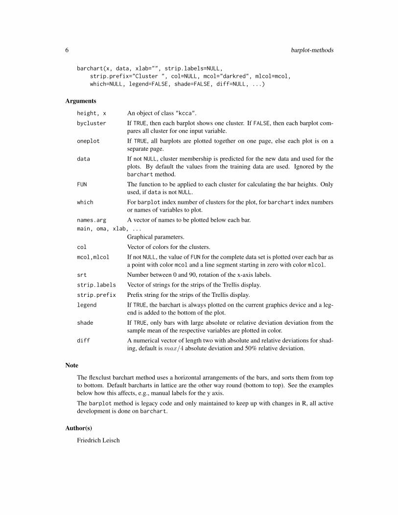
barchart(x, data, xlab="", strip.labels=NULL,strip.prefix="Cluster ", col=NULL, mcol="darkred", mlcol=mcol,which=NULL, legend=FALSE, shade=FALSE, diff=NULL, ...)

Arguments

height, x An object of class "kcca".

bycluster If TRUE, then each barplot shows one cluster. If FALSE, then each barplot com-pares all cluster for one input variable.

oneplot If TRUE, all barplots are plotted together on one page, else each plot is on aseparate page.

data If not NULL, cluster membership is predicted for the new data and used for theplots. By default the values from the training data are used. Ignored by thebarchart method.

FUN The function to be applied to each cluster for calculating the bar heights. Onlyused, if data is not NULL.

which For barplot index number of clusters for the plot, for barchart index numbersor names of variables to plot.

names.arg A vector of names to be plotted below each bar.main, oma, xlab, ...

Graphical parameters.

col Vector of colors for the clusters.

mcol,mlcol If not NULL, the value of FUN for the complete data set is plotted over each bar asa point with color mcol and a line segment starting in zero with color mlcol.

srt Number between 0 and 90, rotation of the x-axis labels.

strip.labels Vector of strings for the strips of the Trellis display.

strip.prefix Prefix string for the strips of the Trellis display.

legend If TRUE, the barchart is always plotted on the current graphics device and a leg-end is added to the bottom of the plot.

shade If TRUE, only bars with large absolute or relative deviation deviation from thesample mean of the respective variables are plotted in color.

diff A numerical vector of length two with absolute and relative deviations for shad-ing, default is max/4 absolute deviation and 50% relative deviation.

Note

The flexclust barchart method uses a horizontal arrangements of the bars, and sorts them from topto bottom. Default barcharts in lattice are the other way round (bottom to top). See the examplesbelow how this affects, e.g., manual labels for the y axis.

The barplot method is legacy code and only maintained to keep up with changes in R, all activedevelopment is done on barchart.

Author(s)

Friedrich Leisch

birth 7

References

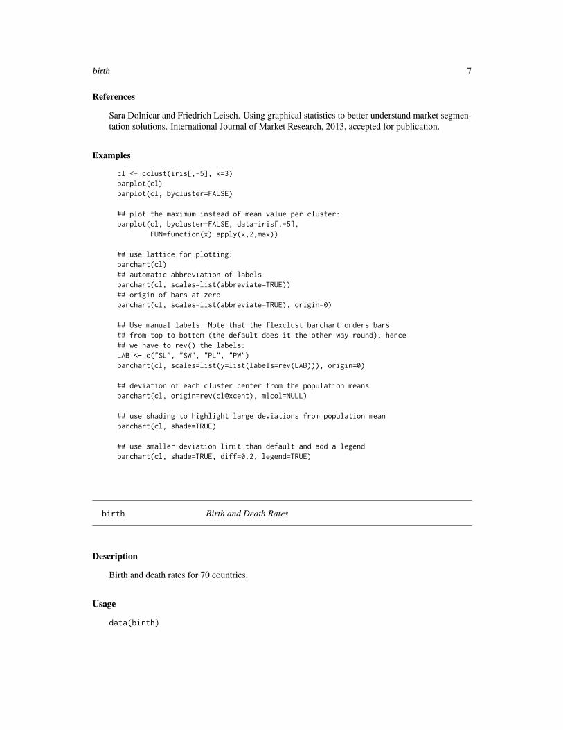
Sara Dolnicar and Friedrich Leisch. Using graphical statistics to better understand market segmen-tation solutions. International Journal of Market Research, 2013, accepted for publication.

Examples

cl <- cclust(iris[,-5], k=3)barplot(cl)barplot(cl, bycluster=FALSE)

## plot the maximum instead of mean value per cluster:barplot(cl, bycluster=FALSE, data=iris[,-5],

FUN=function(x) apply(x,2,max))

## use lattice for plotting:barchart(cl)## automatic abbreviation of labelsbarchart(cl, scales=list(abbreviate=TRUE))## origin of bars at zerobarchart(cl, scales=list(abbreviate=TRUE), origin=0)

## Use manual labels. Note that the flexclust barchart orders bars## from top to bottom (the default does it the other way round), hence## we have to rev() the labels:LAB <- c("SL", "SW", "PL", "PW")barchart(cl, scales=list(y=list(labels=rev(LAB))), origin=0)

## deviation of each cluster center from the population meansbarchart(cl, origin=rev(cl@xcent), mlcol=NULL)

## use shading to highlight large deviations from population meanbarchart(cl, shade=TRUE)

## use smaller deviation limit than default and add a legendbarchart(cl, shade=TRUE, diff=0.2, legend=TRUE)

birth Birth and Death Rates

Description

Birth and death rates for 70 countries.

Usage

data(birth)

8 bootFlexclust

Format


birth: birth rate (in percent)

death: death rate (in percent)

References


bootFlexclust Bootstrap Flexclust Algorithms

Description

Runs clustering algorithms repeatedly for different numbers of clusters on bootstrap replica of theoriginal data and returns corresponding cluster assignments, centroids and Rand indices comparingpairs of partitions.

Usage

bootFlexclust(x, k, nboot=100, correct=TRUE, seed=NULL,multicore=TRUE, verbose=FALSE, ...)

## S4 method for signature 'bootFlexclust'summary(object)## S4 method for signature 'bootFlexclust,missing'plot(x, y, ...)## S4 method for signature 'bootFlexclust'boxplot(x, ...)## S4 method for signature 'bootFlexclust'densityplot(x, data, ...)

Arguments

x, k, ... Passed to stepFlexclust.

nboot Number of bootstrap pairs of partitions.

correct Logical, correct the index for agreement by chance?

seed If not NULL, a call to set.seed() is made before any clustering is done.

multicore If TRUE, use package parallel for parallel processing. In addition, it may be aworkstation cluster object as returned by makeCluster, see examples below.

verbose If TRUE, show progress information during computations. Will not work withmulticore=TRUE.

y, data Not used.

object An object of class "bootFlexclust".

bundestag 9

Details

Availability of multicore is checked when flexclust is loaded and stored in getOption("flexclust")$have_multicore.Set to FALSE for debugging and more sensible error messages in case something goes wrong.

Author(s)

Friedrich Leisch

See Also

stepFlexclust

Examples

## Not run:

## data uniform on unit squarex <- matrix(runif(400), ncol=2)

cl <- FALSE

## to run bootstrap replications on a workstation cluster do the following:library("parallel")cl <- makeCluster(2, type = "PSOCK")clusterCall(cl, function() require("flexclust"))

## 50 bootstrap replicates for speed in example,## use more for real applicationsbcl <- bootFlexclust(x, k=2:7, nboot=50, FUN=cclust, multicore=cl)

bclsummary(bcl)

## splitting the square into four quadrants should be the most stable## solution (increase nboot if not)plot(bcl)densityplot(bcl, from=0)

## End(Not run)

bundestag German Parliament Election Data

Description

Results of the elections 2002, 2005 or 2009 for the German Bundestag, the first chamber of theGerman parliament.

10 bundestag

Usage

data(btw2002)data(btw2005)data(btw2009)bundestag(year, second=TRUE, percent=TRUE, nazero=TRUE, state=FALSE)

Arguments

year numeric or character, year of the election.

second logical, return second or first votes?

percent logical, return percentages or absolute numbers?

nazero logical, convert NAs to 0?

state logical or character. If TRUE then only column state from the correspondingdata frame is returned, and all other arguments are ignored. If character, then itis used as pattern to grep for the corresponding state(s), see examples.

Format

btw200x are data frames with 299 rows (corresponding to constituencies) and 17 columns. Allcolumns except state are numeric.

state: factor, the 16 German federal states.

eligible: number of citizens eligible to vote.

votes: number of eligible citizens who did vote.

invalid1, invalid2: number of invalid first and second votes (see details below).

valid1, valid2: number of valid first and second votes.

SPD1, SPD2: number of first and second votes for the Social Democrats.

UNION1, UNION2: number of first and second votes for CDU/CSU, the conservative ChristianDemocrats.

GRUENE1, GRUENE2: number of first and second votes for the Green Party.

FDP1, FDP2: number of first and second votes for the Liberal Party.

LINKE1, LINKE2: number of first and second votes for the Left Party (PDS in 2002).

Missing values indicate that a party did not candidate in the corresponding constituency.

Details

btw200x are the original data sets. bundestag() is a helper function which extracts first or sec-ond votes, calculates percentages (number of votes for a party divided by number of valid votes),replaces missing values by zero, and converts the result from a data frame to a matrix. By defaultit returns the percentage of second votes for each party, which determines the number of seats eachparty gets in parliament.

bwplot-methods 11

German Federal Elections

Half of the Members of the German Bundestag are elected directly from Germany’s 299 constituen-cies, the other half on the parties’ state lists. Accordingly, each voter has two votes in the electionsto the German Bundestag. The first vote, allowing voters to elect their local representatives to theBundestag, decides which candidates are sent to Parliament from the constituencies.

The second vote is cast for a party list. And it is this second vote that determines the relativestrengths of the parties represented in the Bundestag. At least 598 Members of the German Bun-destag are elected in this way. In addition to this, there are certain circumstances in which somecandidates win what are known as “overhang mandates” when the seats are being distributed.

References

Homepage of the Bundestag: http://www.bundestag.de

Examples

p02 <- bundestag(2002)pairs(p02)p05 <- bundestag(2005)pairs(p05)p09 <- bundestag(2009)pairs(p09)

state <- bundestag(2002, state=TRUE)table(state)

start.with.b <- bundestag(2002, state="^B")table(start.with.b)

pairs(p09, col=2-(state=="Bayern"))

bwplot-methods Box-Whisker Plot Methods in Package ‘flexclust’

Description

Seperate boxplot of variables in each cluster in comparison with boxplot for complete sample.

Usage

## S4 method for signature 'kcca'bwplot(x, data, xlab="",

strip.labels=NULL, strip.prefix="Cluster ",col=NULL, shade=!is.null(shadefun), shadefun=NULL, ...)

http://www.bundestag.de

12 cclust

Arguments

x An object of class "kcca".

data If not NULL, cluster membership is predicted for the new data and used for theplots. By default the values from the training data are used.

xlab, ... Graphical parameters.

col Vector of colors for the clusters.

strip.labels Vector of strings for the strips of the Trellis display.

strip.prefix Prefix string for the strips of the Trellis display.

shade If TRUE, only boxes with larger deviation from the median or quartiles of thetotal population of the respective variables are filled with color.

shadefun A function or name of a function to compute which boxes are shaded, e.g."medianInside" (default) or "boxOverlap".

Examples

set.seed(1)cl <- cclust(iris[,-5], k=3, save.data=TRUE)bwplot(cl)

## fill only boxes with color which do not contain the overall median## (grey dot of background box)bwplot(cl, shade=TRUE)

## fill only boxes with color which do not overlap with the box of the## complete sample (grey background box)bwplot(cl, shadefun="boxOverlap")

cclust Convex Clustering

Description

Perform k-means clustering, hard competitive learning or neural gas on a data matrix.

Usage

cclust(x, k, dist = "euclidean", method = "kmeans",weights=NULL, control=NULL, group=NULL, simple=FALSE,save.data=FALSE)

cclust 13

Arguments

x A numeric matrix of data, or an object that can be coerced to such a matrix (suchas a numeric vector or a data frame with all numeric columns).

k Either the number of clusters, or a vector of cluster assignments, or a matrix ofinitial (distinct) cluster centroids. If a number, a random set of (distinct) rows inx is chosen as the initial centroids.

dist Distance measure, one of "euclidean" (mean square distance) or "manhattan "(absolute distance).

method Clustering algorithm: one of "kmeans", "hardcl" or "neuralgas", see detailsbelow.

weights An optional vector of weights to be used in the fitting process. Works only incombination with hard competitive learning.

control An object of class cclustControl.

group Currently ignored.

simple Return an object of class kccasimple?

save.data Save a copy of x in the return object?

Details

This function uses the same computational engine as the earlier function of the same name frompackage ‘cclust’. The main difference is that it returns an S4 object of class "kcca", hence allavailable methods for "kcca" objects can be used. By default kcca and cclust use exactly thesame algorithm, but cclust will usually be much faster because it uses compiled code.

If dist is "euclidean", the distance between the cluster center and the data points is the Euclidiandistance (ordinary kmeans algorithm), and cluster means are used as centroids. If "manhattan",the distance between the cluster center and the data points is the sum of the absolute values of thedistances, and the column-wise cluster medians are used as centroids.

If method is "kmeans", the classic kmeans algorithm as given by MacQueen (1967) is used, whichworks by repeatedly moving all cluster centers to the mean of their respective Voronoi sets. If"hardcl", on-line updates are used (AKA hard competitive learning), which work by randomlydrawing an observation from x and moving the closest center towards that point (e.g., Ripley 1996).If "neuralgas" then the neural gas algorithm by Martinetz et al (1993) is used. It is similar tohard competitive learning, but in addition to the closest centroid also the second closest centroid ismoved in each iteration.

Value

An object of class "kcca".

Author(s)

Evgenia Dimitriadou and Friedrich Leisch

14 clusterSim

References

MacQueen, J. (1967). Some methods for classification and analysis of multivariate observations.In Proceedings of the Fifth Berkeley Symposium on Mathematical Statistics and Probability, eds L.M. Le Cam \& J. Neyman, 1, pp. 281–297. Berkeley, CA: University of California Press.

Martinetz T., Berkovich S., and Schulten K (1993). ‘Neural-Gas’ Network for Vector Quantizationand its Application to Time-Series Prediction. IEEE Transactions on Neural Networks, 4 (4), pp.558–569.

Ripley, B. D. (1996) Pattern Recognition and Neural Networks. Cambridge.

See Also

cclustControl-class, kcca

Examples

## a 2-dimensional examplex<-rbind(matrix(rnorm(100,sd=0.3),ncol=2),

matrix(rnorm(100,mean=1,sd=0.3),ncol=2))cl<-cclust(x,2)plot(x, col=predict(cl))points(cl@centers, pch="x", cex=2, col=3)

## a 3-dimensional examplex<-rbind(matrix(rnorm(150,sd=0.3),ncol=3),

matrix(rnorm(150,mean=2,sd=0.3),ncol=3),matrix(rnorm(150,mean=4,sd=0.3),ncol=3))

cl<-cclust(x, 6, method="neuralgas", save.data=TRUE)pairs(x, col=predict(cl))plot(cl)

clusterSim Cluster Similarity Matrix

Description

Returns a matrix of cluster similarities. Currently two methods for computing similarities of clustersare implemented, see details below.

Usage

## S4 method for signature 'kcca'clusterSim(object, data=NULL, method=c("shadow", "centers"),

symmetric=FALSE, ...)## S4 method for signature 'kccasimple'clusterSim(object, data=NULL, method=c("shadow", "centers"),

symmetric=FALSE, ...)

clusterSim 15

Arguments

object fitted object.

data Data to use for computation of the shadow values. If the cluster object x was cre-ated with save.data=TRUE, then these are used by default. Ignored if method="centers".

method Type of similarities, see details below.

symmetric Compute symmetric or asymmetric shadow values? Ignored if method="centers".

... currently not used.

Details

If method="shadow" (the default), then the similarity of two clusters is proportional to the numberof points in a cluster, where the centroid of the other cluster is second-closest. See Leisch (2006,2008) for detailed formulas.

If method="centers", then first the pairwise distances between all centroids are computed andrescaled to [0,1]. The similarity between tow clusters is then simply 1 minus the rescaled distance.

Author(s)

Friedrich Leisch

References

Friedrich Leisch. A Toolbox for K-Centroids Cluster Analysis. Computational Statistics and DataAnalysis, 51 (2), 526–544, 2006.

Friedrich Leisch. Visualizing cluster analysis and finite mixture models. In Chun houh Chen, Wolf-gang Haerdle, and Antony Unwin, editors, Handbook of Data Visualization, Springer Handbooksof Computational Statistics. Springer Verlag, 2008.

Examples

example(Nclus)

clusterSim(cl)clusterSim(cl, symmetric=TRUE)

## should have similar structure but will be numerically different:clusterSim(cl, symmetric=TRUE, data=Nclus[sample(1:550, 200),])

## different concept of cluster similarityclusterSim(cl, method="centers")

16 conversion

conversion Conversion Between S3 Partition Objects and KCCA

Description

These functions can be used to convert the results from cluster functions like kmeans or pam toobjects of class "kcca" and vice versa

Usage

as.kcca(object, ...)

## S3 method for class 'hclust'as.kcca(object, data, k, family=NULL, save.data=FALSE, ...)## S3 method for class 'kmeans'as.kcca(object, data, save.data=FALSE, ...)## S3 method for class 'partition'as.kcca(object, data=NULL, save.data=FALSE, ...)## S3 method for class 'skmeans'as.kcca(object, data, save.data=FALSE, ...)## S4 method for signature 'kccasimple,kmeans'coerce(from, to="kmeans", strict=TRUE)

Arguments


data data which were used to obtain the clustering. For "partition" objects createdby functions from package cluster this is optional, if object contains the data.

save.data Save a copy of the data in the return object?

k number of clusters.

family object of class kccaFamily, can be omitted for some known distances.

... currently not used.from, to, strict

usual arguments for coerce

Details

For hierarchical clustering the cluster memberships of the converted object can be different fromthe result of cutree, because one KCCA-iteration has to be performed in order to obtain a validkcca object. In this case a warning is issued.

Author(s)

Friedrich Leisch

dentitio 17

Examples

data(Nclus)

cl1 <- kmeans(Nclus, 4)cl1cl1a <- as.kcca(cl1, Nclus)cl1acl1b <- as(cl1a, "kmeans")

library("cluster")cl2 <- pam(Nclus, 4)cl2cl2a <- as.kcca(cl2)cl2a## the samecl2b = as.kcca(cl2, Nclus)cl2b

## hierarchical clusteringhc <- hclust(dist(USArrests))plot(hc)rect.hclust(hc, k=3)c3 <- cutree(hc, k=3)k3 <- as.kcca(hc, USArrests, k=3)barchart(k3)table(c3, clusters(k3))

dentitio Dentition of Mammals

Description

Mammal’s teeth divided into the 4 groups: incisors, canines, premolars and molars.

Usage

data(dentitio)

Format


top.inc: top incisors

bot.inc: bottom incisors

top.can: top canines

18 dist2

bot.can: bottom canines

top.pre: top premolars

bot.pre: bottom premolars

top.mol: top molars

bot.mol: bottom molars

References


dist2 Compute pairwise distances between two data sets

Description

This function computes and returns the distance matrix computed by using the specified distancemeasure to compute the pairwise distances between the rows of two data matrices.

Usage

dist2(x, y, method = "euclidean", p=2)

Arguments

x A data matrix.

y A vector or second data matrix.

method the distance measure to be used. This must be one of "euclidean", "maximum","manhattan", "canberra", "binary" or "minkowski". Any unambiguoussubstring can be given.

p The power of the Minkowski distance.

Details

This is a two-data-set equivalent of the standard function dist. It returns a matrix of all pairwisedistances between rows in x and y. The current implementation is efficient only if y has not toomany rows (the code is vectorized in x but not in y).

Note

The definition of Canberra distance was wrong for negative data prior to version 1.3-5.

Author(s)

Friedrich Leisch

distances 19

See Also

dist

Examples

x = matrix(rnorm(20), ncol=4)rownames(x) = paste("X", 1:nrow(x), sep=".")y = matrix(rnorm(12), ncol=4)rownames(y) = paste("Y", 1:nrow(y), sep=".")

dist2(x, y)dist2(x, y, "man")

data(milk)dist2(milk[1:5,], milk[4:6,])

distances Distance and Centroid Computation

Description

Helper functions to create kccaFamily objects.

Usage

distAngle(x, centers)distCanberra(x, centers)distCor(x, centers)distEuclidean(x, centers)distJaccard(x, centers)distManhattan(x, centers)distMax(x, centers)distMinkowski(x, centers, p=2)

centAngle(x)centMean(x)centMedian(x)

centOptim(x, dist)centOptim01(x, dist)

Arguments

x A data matrix.

centers A matrix of centroids.

p The power of the Minkowski distance.

dist A distance function.

20 flexclustControl-class

Author(s)

Friedrich Leisch

flexclustControl-class

Classes "flexclustControl" and "cclustControl"

Description

Hyperparameters for cluster algorithms.

Objects from the Class

Objects can be created by calls of the form new("flexclustControl", ...). In addition, namedlists can be coerced to flexclustControl objects, names are completed if unique (see examples).

Slots

Objects of class flexclustControl have the following slots:

iter.max: Maximum number of iterations.

tolerance: The algorithm is stopped when the (relative) change of the optimization criterion issmaller than tolerance.

verbose: If a positive integer, then progress is reported every verbose iterations. If 0, no output isgenerated during model fitting.

classify: Character string, one of "auto", "weighted", "hard" or "simann".

initcent: Character string, name of function for initial centroids, currently "randomcent" (thedefault) and "kmeanspp" are available.

gamma: Gamma value for weighted hard competitive learning.

simann: Parameters for simulated annealing optimization (only used when classify="simann").

ntry: Number of trials per iteration for QT clustering.

min.size: Clusters smaller than this value are treated as outliers.

Objects of class cclustControl inherit from flexclustControl and have the following additionalslots:

method: Learning rate for hard competitive learning, one of "polynomial" or "exponential".

pol.rate: Positive number for polynomial learning rate of form 1/iterpar.

exp.rate Vector of length 2 with parameters for exponential learning rate of form par1∗(par2/par1)(iter/iter.max).

ng.rate: Vector of length 4 with parameters for neural gas, see details below.

flexclustControl-class 21

Learning Rate of Neural Gas

The neural gas algorithm uses updates of form

cnew = cold+ e ∗ exp(−m/l) ∗ (x− cold)

for every centroid, where m is the order (minus 1) of the centroid with respect to distance to datapoint x (0=closest, 1=second, . . . ). The parameters e and l are given by

e = par1 ∗ (par2/par1)(iter/iter.max),

l = par3 ∗ (par4/par3)(iter/iter.max).

See Martinetz et al (1993) for details of the algorithm, and the examples section on how to obtaindefault values.

Author(s)

Friedrich Leisch

References

Martinetz T., Berkovich S., and Schulten K. (1993). "Neural-Gas Network for Vector Quantizationand its Application to Time-Series Prediction." IEEE Transactions on Neural Networks, 4 (4), pp.558–569.

Arthur D. and Vassilvitskii S. (2007). "k-means++: the advantages of careful seeding". Proceedingsof the 18th annual ACM-SIAM symposium on Discrete algorithms. pp. 1027-1035.

See Also

kcca, cclust

Examples

## have a look at the defaultsnew("flexclustControl")

## corce a listmycont = list(iter=500, tol=0.001, class="w")as(mycont, "flexclustControl")

## some additional slotsas(mycont, "cclustControl")

## default values for ng.ratenew("cclustControl")@ng.rate

22 flxColors

flxColors Flexclust Color Palettes

Description

Create and access palettes for the plot methods.

Usage

flxColors(n=1:8, color=c("full","medium", "light","dark"), grey=FALSE)

Arguments

n Index number of color to return (1 to 8)

color Type of color, see details.

grey Return grey value corresponding to palette.

Details

This function creates color palettes in HCL space for up to 8 colors. All palettes have constantchroma and luminance, only the hue of the colors change within a palette.

Palettes "full" and "dark" have the same luminance, and palettes "medium" and "light" havethe same luminance.

Author(s)

Friedrich Leisch

See Also

hcl

Examples

opar <- par(c("mfrow", "mar", "xaxt"))par(mfrow=c(2,2), mar=c(0,0,2,0), yaxt="n")

x <- rep(1, 8)

barplot(x, col = flxColors(color="full"), main="full")barplot(x, col = flxColors(color="dark"), main="dark")barplot(x, col = flxColors(color="medium"), main="medium")barplot(x, col = flxColors(color="light"), main="light")

par(opar)

image-methods 23

image-methods Methods for Function image in Package ‘flexclust’

Description

Image plot of cluster segments overlaid by neighbourhood graph.

Usage

## S4 method for signature 'kcca'image(x, which = 1:2, npoints = 100,

xlab = "", ylab = "", fastcol = TRUE, col=NULL,clwd=0, graph=TRUE, ...)

Arguments

x An object of class "kcca".

which Index number of dimensions of input space to plot.

npoints Number of grid points for image.

fastcol If TRUE, a greedy algorithm is used for the background colors of the segments,which may result in neighbouring segments having the same color. If FALSE,neighbouring segments always have different colors at a speed penalty.

col Vector of background colors for the segments.

clwd Line width of contour lines at cluster boundaries, use larger values for npointsthan the default to get smooth lines. (Warning: We really need a smarter way todraw cluster boundaries!)

graph Logical, add a neighborhood graph to the plot?xlab, ylab, ...

Graphical parameters.

Details

This works only for "kcca" objects, no method is available for "kccasimple" objects.

Author(s)

Friedrich Leisch

See Also

kcca

24 info

info Get Information on Fitted Flexclust Objects

Description

Returns descriptive information about fitted flexclust objects like cluster sizes or sum of within-cluster distances.

Usage

## S4 method for signature 'flexclust,character'info(object, which, drop=TRUE, ...)

Arguments


which which information to get. Use which="help" to list available information.

drop logical. If TRUE the result is coerced to the lowest possible dimension.

... passed to methods.

Details

Function info can be used to access slots of fitted flexclust objects in a portable way, and in additioncomputes some meta-information like sum of within-cluster distances.

Function infoCheck returns a logical value that is TRUE if the requested information can be com-puted from the object.

Author(s)

Friedrich Leisch

See Also

info

Examples

data("Nclus")plot(Nclus)

cl1 = cclust(Nclus, k=4)summary(cl1)

## these two are the sameinfo(cl1)info(cl1, "help")

kcca 25

## cluster sizesi1 = info(cl1, "size")i1

## average within cluster distancesi2 = info(cl1, "av_dist")i2

## the sum of all within-cluster distancesi3 = info(cl1, "distsum")i3

## sum(i1*i2) must of course be the same as i3stopifnot(all.equal(sum(i1*i2), i3))

## This should return TRUEinfoCheck(cl1, "size")## and this FALSEinfoCheck(cl1, "Homer Simpson")## both combinedi4 = infoCheck(cl1, c("size", "Homer Simpson"))i4

stopifnot(all.equal(i4, c(TRUE, FALSE)))

kcca K-Centroids Cluster Analysis

Description

Perform k-centroids clustering on a data matrix.

Usage

kcca(x, k, family=kccaFamily("kmeans"), weights=NULL, group=NULL,control=NULL, simple=FALSE, save.data=FALSE)

kccaFamily(which=NULL, dist=NULL, cent=NULL, name=which,preproc = NULL, trim=0, groupFun = "minSumClusters")

## S4 method for signature 'kccasimple'summary(object)

Arguments


26 kcca

k Either the number of clusters, or a vector of cluster assignments, or a matrix ofinitial (distinct) cluster centroids. If a number, a random set of (distinct) rows inx is chosen as the initial centroids.

family Object of class kccaFamily.

weights An optional vector of weights to be used in the clustering process, cannot becombined with all families.

group An optional grouping vector for the data, see details below.

control An object of class flexclustControl.



which One of "kmeans", "kmedians", "angle", "jaccard", or "ejaccard".

name Optional long name for family, used only for show methods.

dist A function for distance computation, ignored if which is specified.

cent A function for centroid computation, ignored if which is specified.

preproc Function for data preprocessing.

trim A number in between 0 and 0.5, if non-zero then trimmed means are used forthe kmeans family, ignored by all other families.

groupFun Function or name of function to obtain clusters for grouped data, see detailsbelow.

object Object of class "kcca".

Details

See the paper A Toolbox for K-Centroids Cluster Analysis referenced below for details.

Value

Function kcca returns objects of class "kcca" or "kccasimple" depending on the value of argu-ment simple. The simpler objects contain fewer slots and hence are faster to compute, but containno auxiliary information used by the plotting methods. Most plot methods for "kccasimple" ob-jects do nothing and return a warning. If only centroids, cluster membership or prediction for newdata are of interest, then the simple objects are sufficient.

Predefined Families

Function kccaFamily() currently has the following predefined families (distance / centroid):

kmeans: Euclidean distance / mean

kmedians: Manhattan distance / median

angle: angle between observation and centroid / standardized mean

jaccard: Jaccard distance / numeric optimization

ejaccard: Jaccard distance / mean

See Leisch (2006) for details on all combinations.

kcca 27

Group Constraints

If group is not NULL, then observations from the same group are restricted to belong to the samecluster (must-link constraint) or different clusters (cannot-link constraint) during the fitting process.If groupFun = "minSumClusters", then all group members are assign to the cluster where thecenter has minimal average distance to the group members. If groupFun = "majorityClusters",then all group members are assigned to the cluster the majority would belong to without a constraint.

groupFun = "differentClusters" implements a cannot-link constraint, i.e., members of onegroup are not allowed to belong to the same cluster. The optimal allocation for each group is foundby solving a linear sum assignment problem using solve_LSAP. Obviously the group sizes must besmaller than the number of clusters in this case.

Ties are broken at random in all cases. Note that at the moment not all methods for fitted "kcca"objects respect the grouping information, most importantly the plot method when a data argumentis specified.

Author(s)

Friedrich Leisch

References

Friedrich Leisch. A Toolbox for K-Centroids Cluster Analysis. Computational Statistics and DataAnalysis, 51 (2), 526–544, 2006.

Friedrich Leisch and Bettina Gruen. Extending standard cluster algorithms to allow for group con-straints. In Alfredo Rizzi and Maurizio Vichi, editors, Compstat 2006-Proceedings in Computa-tional Statistics, pages 885-892. Physica Verlag, Heidelberg, Germany, 2006.

See Also

stepFlexclust, cclust, distances

Examples


## try kmeanscl1 = kcca(Nclus, k=4)cl1

image(cl1)points(Nclus)

## A barplot of the centroidsbarplot(cl1)

## now use k-medians and kmeans++ initialization, cluster centroids## should be similar...

28 milk

cl2 = kcca(Nclus, k=4, family=kccaFamily("kmedians"),control=list(initcent="kmeanspp"))

cl2

## ... but the boundaries of the partitions have a different shapeimage(cl2)points(Nclus)

kcca2df Convert Cluster Result to Data Frame

Description

Convert object of class "kcca" to a data frame in long format.

Usage

kcca2df(object, data)

Arguments

object Object of class "kcca".

data Optional data if not saved in object.

Value

A data.frame with columns value, variable and group.

Examples

c.iris <- cclust(iris[,-5], 3, save.data=TRUE)df.c.iris <- kcca2df(c.iris)summary(df.c.iris)densityplot(~value|variable+group, data=df.c.iris)

milk Milk of Mammals

Description

The data set contains the ingredients of mammal’s milk of 25 animals.

Usage

data(milk)

Nclus 29

Format

A data frame with 25 observations on the following 5 variables (all in percent).

water: water

protein: protein

fat: fat

lactose: lactose

ash: ash

References


Nclus Artificial Example with 4 Gaussians

Description

A simple artificial regression example with 4 clusters, all of them having a Gaussian distribution.

Usage

data(Nclus)

Details

The Nclus data set can be re-created by loading package flexmix and running ExNclus(100) usingset.seed(2602). It has been saved as a data set for simplicity of examples only.

Examples

data(Nclus)cl <- cclust(Nclus, k=4, simple=FALSE, save.data=TRUE)plot(cl)

30 pairs-methods

nutrient Nutrients in Meat, Fish and Fowl

Description

The data set contains the measurements of nutrients in several types of meat, fish and fowl.

Usage

data(nutrient)

Format


energy: food energy (calories)

protein: protein (grams)

fat: fat (grams)

calcium: calcium (milli grams)

iron: iron (milli grams)

References


pairs-methods Methods for Function pairs in Package ‘flexclust’

Description

Plot a matrix of neighbourhood graphs.

Usage

## S4 method for signature 'kcca'pairs(x, which=NULL, project=NULL, oma=NULL, ...)

Arguments

x an object of class "kcca"

which Index numbers of dimensions of (projected) input space to plot, default is to plotall dimensions.

project Projection object for which a predict method exists, e.g., the result of prcomp.

oma Outer margin.

... Passed to the plot method.

parameters 31

Details


Author(s)

Friedrich Leisch

parameters Get Centroids from KCCA Object

Description

Returns the matrix of centroids of a fitted object of class "kcca".

Usage

## S4 method for signature 'kccasimple'parameters(object, ...)

Arguments



Author(s)

Friedrich Leisch

plot-methods Methods for Function plot in Package ‘flexclust’

Description

Plot the neighbourhood graph of a cluster solution together with projected data points.

Usage

## S4 method for signature 'kcca,missing'plot(x, y, which=1:2, project=NULL,

data=NULL, points=TRUE, hull=TRUE, hull.args=NULL,number = TRUE, simlines=TRUE,lwd=1, maxlwd=8*lwd, cex=1.5, numcol=FALSE, nodes=16,add=FALSE, xlab="", ylab="", xlim = NULL,ylim = NULL, pch=NULL, col=NULL, ...)

32 plot-methods

Arguments

x an object of class "kcca"

y not used

which Index numbers of dimensions of (projected) input space to plot.

project Projection object for which a predict method exists, e.g., the result of prcomp.

data Data to include in plot. If the cluster object x was created with save.data=TRUE,then these are used by default.

points Logical, shall data points be plotted (if available)?

hull If TRUE, then hulls of the data are plotted (if available). Can either be a logicalvalue, one of the strings "convex" (the default) or "ellipse", or a function forplotting the hulls.

hull.args A list of arguments for the hull function.

number Logical, plot number labels in nodes of graph?

numcol, cex Color and size of number labels in nodes of graph. If numcol is logical, itswitches between black and the color of the clusters, else it is taken as a vectorof colors.

nodes Plotting symbol to use for nodes if no numbers are drawn.

simlines Logical, plot edges of graph?

lwd, maxlwd Numerical, thickness of lines.

add Logical, add to existing plot?

xlab, ylab Axis labels.

xlim, ylim Axis range.

pch, col, ... Plotting symbols and colors for data points.

Details


Author(s)

Friedrich Leisch

References

Friedrich Leisch. Visualizing cluster analysis and finite mixture models. In Chun houh Chen, Wolf-gang Haerdle, and Antony Unwin, editors, Handbook of Data Visualization, Springer Handbooksof Computational Statistics. Springer Verlag, 2008.

predict-methods 33

predict-methods Predict Cluster Membership

Description

Return either the cluster membership of training data or predict for new data.

Usage

## S4 method for signature 'kccasimple'predict(object, newdata, ...)## S4 method for signature 'flexclust,ANY'clusters(object, newdata, ...)

Arguments

object Object of class inheriting from "flexclust".

newdata An optional data matrix with the same number of columns as the cluster centers.If omitted, the fitted values are used.

... Currently not used.

Details

clusters can be used on any object of class "flexclust" and returns the cluster memberships ofthe training data.

predict can be used only on objects of class "kcca" (which inherit from "flexclust"). If nonewdata argument is specified, the function is identical to clusters, if newdata is specified, thencluster memberships for the new data are predicted. clusters(object, newdata, ...) is analias for predict(object, newdata, ...).

Author(s)

Friedrich Leisch

priceFeature Artificial 2d Market Segment Data

Description

Simple artificial 2-dimensional data to demonstrate clustering for market segmentation. One di-mension is the hypothetical feature sophistication (or performance or quality, etc) of a product, thesecond dimension the price customers are willing to pay for the product.

34 projAxes

Usage

priceFeature(n, which=c("2clust", "3clust", "5clust","ellipse", "triangle", "circle", "square","largesmall"))

Arguments

n sample size

which shape of data set

References

Sara Dolnicar and Friedrich Leisch. Evaluation of structure and reproducibility of cluster solutionsusing the bootstrap. Marketing Letters, 21:83-101, 2010.

Examples

plot(priceFeature(200, "2clust"))plot(priceFeature(200, "3clust"))plot(priceFeature(200, "5clust"))plot(priceFeature(200, "ell"))plot(priceFeature(200, "tri"))plot(priceFeature(200, "circ"))plot(priceFeature(200, "square"))plot(priceFeature(200, "largesmall"))

projAxes Add Arrows for Projected Axes to a Plot

Description

Adds arrows for original coordinate axes to a projection plot.

Usage

projAxes(object, which=1:2, center=NULL,col="red", radius=NULL,minradius=0.1, textargs=list(col=col),col.names=getColnames(object),which.names="", group = NULL, groupFun = colMeans,plot=TRUE, ...)

placeLabels(object)## S4 method for signature 'projAxes'placeLabels(object)

projAxes 35

Arguments

object Return value of a projection method like prcomp.

which Index number of dimensions of (projected) input space that have been plotted.

center Center of the coordinate system to use in projected space. Default is the centerof the plotting region.

col Color of arrows.

radius Relative size of the arrows.

minradius Minimum radius of arrows to include (relative to arrow size).

textargs List of arguments for text.

col.names Variable names of the original data.

which.names A regular expression which variable names to include in the plot.

group An optional grouping variable for the original coordinates. Coordinates withgroup NA are omitted.

groupFun Function used to aggregate the projected coordinates if group is specified.

plot Logical,if TRUE the axes are added to the current plot.

... Passed to arrows.

Value

projAxes invisibly returns an object of class "projAxes", which can be added to an existing plotby its plot method.

Author(s)

Friedrich Leisch

Examples

data(milk)milk.pca <- prcomp(milk, scale=TRUE)

## create a biplot step by stepplot(predict(milk.pca), type="n")text(predict(milk.pca), rownames(milk), col="green", cex=0.8)projAxes(milk.pca)

## the same, but arrows are blue, centered at origin and all arrows are## plottedplot(predict(milk.pca), type="n")text(predict(milk.pca), rownames(milk), col="green", cex=0.8)projAxes(milk.pca, col="blue", center=0, minradius=0)

## use points instead of text, plot PC2 and PC3, manual radius## specification, store resultplot(predict(milk.pca)[,c(2,3)])arr <- projAxes(milk.pca, which=c(2,3), radius=1.2, plot=FALSE)

36 propBarchart

plot(arr)

## Not run:

## manually try to find new places for the labels: each arrow is marked## active in turn, use the left mouse button to find a better location## for the label. Use the right mouse button to go on to the next## variable.

arr1 <- placeLabels(arr)

## now do the plot again:plot(predict(milk.pca)[,c(2,3)])plot(arr1)

## End(Not run)

propBarchart Barcharts and Boxplots for Columns of a Data Matrix Split by Groups

Description

Split a binary or numeric matrix by a grouping variable, run a series of tests on all variables, adjustfor multiple testing and graphically represent results.

Usage

propBarchart(x, g, alpha=0.05, correct="holm", test="prop.test",sort=FALSE, strip.prefix="", strip.labels=NULL,which=NULL, ...)

## S4 method for signature 'propBarchart'summary(object, ...)

groupBWplot(x, g, alpha=0.05, correct="holm", col=NULL,shade=!is.null(shadefun), shadefun=NULL,strip.prefix="", strip.labels=NULL, which=NULL, ...)

Arguments

x A binary data matrix.

g A factor specifying the groups.

alpha Significance level for test of differences in proportions.

correct Correction method for multiple testing, passed to p.adjust.

test Test to use for detecting significant differences in proportions.

sort Logical, sort variables by total sample mean?

propBarchart 37

strip.prefix Character string prepended to strips of the barchart (the remainder of the stripare group levels and group sizes). Ignored if strip.labels is specified.

strip.labels Character vector of labels to use for strips of barchart.

which Index numbers or names of variables to plot.

... Passed on to barchart or bwplot.

object Return value of propBarchart.

col Vector of colors for the panels.

shade If TRUE, only variables with significant differences in median are filled withcolor.

shadefun A function or name of a function to compute which boxes are shaded, e.g."kruskalTest" (default), "medianInside" or "boxOverlap".

Details

Function propBarchart splits a binary data matrix into subgroups, computes the percentage of onesin each column and compares the proportions in the groups using prop.test. The p-values for allvariables are adjusted for multiple testing and a barchart of group percentages is drawn highlightingvariables with significant differences in proportion. The summary method can be used to create acorresponding table for publications.

Function groupBWplot takes a general numeric matrix, also splits into subgroups and uses boxesinstead of bars. By default kruskal.test is used to compute significant differences in location, inaddition the heuristics from bwplot,kcca-method can be used. Boxes of the complete sample areused as reference in the background.

Author(s)

Friedrich Leisch

See Also

barplot-methods, bwplot,kcca-method

Examples

## create a binary matrix from the iris data plus a random noise columnx <- apply(iris[,-5], 2, function(z) z>median(z))x <- cbind(x, Noise=sample(0:1, 150, replace=TRUE))

## There are significant differences in all 4 original variables, Noise## has most likely no significant difference (of course the difference## will be significant in alpha percent of all random samples).p <- propBarchart(x, iris$Species)psummary(p)

x <- iris[,-5]x <- cbind(x, Noise=rnorm(150, mean=3))groupBWplot(x, iris$Species)

38 qtclust

groupBWplot(x, iris$Species, shade=TRUE)groupBWplot(x, iris$Species, shadefun="medianInside")

qtclust Stochastic QT Clustering

Description

Perform stochastic QT clustering on a data matrix.

Usage

qtclust(x, radius, family = kccaFamily("kmeans"), control = NULL,save.data=FALSE, kcca=FALSE)

Arguments


radius Maximum radius of clusters.

family Object of class kccaFamily specifying the distance measure to be used.

control An object of class flexclustControl specifying the minimum number of ob-servations per cluster (min.size), and trials per iteration (ntry, see details be-low)..


kcca Run kcca after the QT cluster algorithm has converged?

Details

This function implements a variation of the QT clustering algorithm by Heyer et al. (1999), seeScharl and Leisch (2006). The main difference is that in each iteration not all possible cluster startpoints are considered, but only a random sample of size control@ntry. We also consider onlypoints as initial centers where at least one other point is within a circle with radius radius. In mostcases the resulting solutions are almost the same at a considerable speed increase, in some caseseven better solutions are obtained than with the original algorithm. If control@ntry is set to thesize of the data set, an algorithm similar to the original algorithm as proposed by Heyer et al. (1999)is obtained.

Value

Function qtclust by default returns objects of class "kccasimple". If argument kcca is TRUE,function kcca() is run afterwards (initialized on the QT cluster solution). Data points not clusteredby the QT cluster algorithm are omitted from the kcca() iterations, but filled back into the returnobject. All plot methods defined for objects of class "kcca" can be used.

randIndex 39

Author(s)

Friedrich Leisch

References

Heyer, L. J., Kruglyak, S., Yooseph, S. (1999). Exploring expression data: Identification and anal-ysis of coexpressed genes. Genome Research 9, 1106–1115.

Theresa Scharl and Friedrich Leisch. The stochastic QT-clust algorithm: evaluation of stability andvariance on time-course microarray data. In Alfredo Rizzi and Maurizio Vichi, editors, Compstat2006 – Proceedings in Computational Statistics, pages 1015-1022. Physica Verlag, Heidelberg,Germany, 2006.

Examples

x <- matrix(10*runif(1000), ncol=2)

## maximum distrance of point to cluster center is 3cl1 <- qtclust(x, radius=3)

## maximum distrance of point to cluster center is 1## -> more clusters, longer runtimecl2 <- qtclust(x, radius=1)

opar <- par(c("mfrow","mar"))par(mfrow=c(2,1), mar=c(2.1,2.1,1,1))plot(x, col=predict(cl1), xlab="", ylab="")plot(x, col=predict(cl2), xlab="", ylab="")par(opar)

randIndex Compare Partitions

Description

Compute the (adjusted) Rand, Jaccard and Fowlkes-Mallows index for agreement of two partitions.

Usage

comPart(x, y, type=c("ARI","RI","J","FM"))## S4 method for signature 'flexclust,flexclust'comPart(x, y, type)## S4 method for signature 'numeric,numeric'comPart(x, y, type)## S4 method for signature 'flexclust,numeric'comPart(x, y, type)## S4 method for signature 'numeric,flexclust'comPart(x, y, type)

40 randIndex

randIndex(x, y, correct=TRUE, original=!correct)## S4 method for signature 'table,missing'randIndex(x, y, correct=TRUE, original=!correct)## S4 method for signature 'ANY,ANY'randIndex(x, y, correct=TRUE, original=!correct)

Arguments

x Either a 2-dimensional cross-tabulation of cluster assignments (for randIndexonly), an object inheriting from class "flexclust", or an integer vector of clus-ter memberships.

y An object inheriting from class "flexclust", or an integer vector of clustermemberships.

type character vector of abbreviations of indices to compute.correct, original

Logical, correct the Rand index for agreement by chance?

Value

A vector of indices.

Rand Index

Let A denote the number of all pairs of data points which are either put into the same cluster byboth partitions or put into different clusters by both partitions. Conversely, let D denote the numberof all pairs of data points that are put into one cluster in one partition, but into different clusters bythe other partition. The partitions disagree for all pairs D and agree for all pairs A. We can measurethe agreement by the Rand index A/(A + D) which is invariant with respect to permutations ofcluster labels.

The index has to be corrected for agreement by chance if the sizes of the clusters are not uniform(which is usually the case), or if there are many clusters, see Hubert \& Arabie (1985) for details.

Jaccard Index

If the number of clusters is very large, then usually the vast majority of pairs of points will not bein the same cluster. The Jaccard index tries to account for this by using only pairs of points that arein the same cluster in the defintion of A.

Fowlkes-Mallows

Let A again be the pairs of points that are in the same cluster in both partitions. Fowlkes-Mallowsdivides this number by the geometric mean of the sums of the number of pairs in each cluster of thetwo partitions. This gives the probability that a pair of points which are in the same cluster in onepartition are also in the same cluster in the other partition.

Author(s)

Friedrich Leisch

randomTour 41

References

Lawrence Hubert and Phipps Arabie. Comparing partitions. Journal of Classification, 2, 193–218,1985.

Marina Meila. Comparing clusterings - an axiomatic view. In Stefan Wrobel and Luc De Raedt,editors, Proceedings of the International Machine Learning Conference (ICML). ACM Press, 2005.

Examples

## no class correlations: corrected Rand almost zerog1 <- sample(1:5, size=1000, replace=TRUE)g2 <- sample(1:5, size=1000, replace=TRUE)tab <- table(g1, g2)randIndex(tab)

## uncorrected version will be large, because there are many points## which are assigned to different clusters in both casesrandIndex(tab, correct=FALSE)comPart(g1, g2)

## let pairs (g1=1,g2=1) and (g1=3,g2=3) agree betterk <- sample(1:1000, size=200)g1[k] <- 1g2[k] <- 1k <- sample(1:1000, size=200)g1[k] <- 3g2[k] <- 3tab <- table(g1, g2)

## the index should be larger than beforerandIndex(tab, correct=TRUE, original=TRUE)comPart(g1, g2)

randomTour Plot a Random Tour

Description

Create a series of projection plots corresponding to a random tour through the data.

Usage

randomTour(object, ...)

## S4 method for signature 'ANY'randomTour(object, ...)## S4 method for signature 'matrix'randomTour(object, ...)## S4 method for signature 'flexclust'

42 randomTour

randomTour(object, data=NULL, col=NULL, ...)

randomTourMatrix(x, directions=10,steps=100, sec=4, sleep = sec/steps,axiscol=2, axislab=colnames(x),center=NULL, radius=1, minradius=0.01, asp=1,...)

Arguments

object, x A matrix or an object of class "flexclust".

data Data to include in plot.

col Plotting colors for data points.

directions Integer value, how many different directions are toured.

steps Integer, number of steps in each direction.

sec Numerical, lower bound for the number of seconds each direction takes.

sleep Numerical, sleep for as many seconds after each picture has been plotted.

axiscol If not NULL, then arrows are plotted for projections of the original coordinateaxes in these colors.

axislab Optional labels for the projected axes.

center Center of the coordinate system to use in projected space. Default is the centerof the plotting region.

radius Relative size of the arrows.

minradius Minimum radius of arrows to include.

asp, ... Passed on to randomTourMatrix and from there to plot.

Details

Two random locations are chosen, and data then projected onto hyperplanes which are orthogonalto step vectors interpolating the two locations. The first two coordinates of the projected data areplotted. If directions is larger than one, then after the first steps plots one more random locationis chosen, and the procedure is repeated from the current position to the new location, etc..

The whole procedure is similar to a grand tour, but no attempt is made to optimize subsequentdirections, randomTour simply chooses a random direction in each iteration. Use rggobi for thereal thing.

Obviously the function needs a reasonably fast computer and graphics device to give a smoothimpression, for x11 it may be necessary to use type="Xlib" rather than cairo.

Author(s)

Friedrich Leisch

shadow 43

Examples

if(interactive()){par(ask=FALSE)randomTour(iris[,1:4], axiscol=2:5)randomTour(iris[,1:4], col=as.numeric(iris$Species), axiscol=4)

x <- matrix(runif(300), ncol=3)x <- rbind(x, x+1, x+2)cl <- cclust(x, k=3, save.data=TRUE)

randomTour(cl, center=0, axiscol="black")

## now use predicted cluster membership for new data as colorsrandomTour(cl, center=0, axiscol="black",

data=matrix(rnorm(3000, mean=1, sd=2), ncol=3))}

shadow Cluster shadows and silhouettes

Description

Compute and plot shadows and silhouettes.

Usage

## S4 method for signature 'kccasimple'shadow(object, ...)## S4 method for signature 'kcca'Silhouette(object, data=NULL, ...)

Arguments

object an object of class "kcca" or "kccasimple".

data data to compute silhouette values for. If the cluster object was created withsave.data=TRUE, then these are used by default.


Details

The shadow value of each data point is defined as twice the distance to the closest centroid dividedby the sum of distances to closest and second-closest centroid. If the shadow values of a point isclose to 0, then the point is close to its cluster centroid. If the shadow value is close to 1, it is almostequidistant to the two centroids. Thus, a cluster that is well separated from all other clusters shouldhave many points with small shadow values.

The silhouette value of a data point is defined as the scaled difference between the average dissimi-larity of a point to all points in its own cluster to the smallest average dissimilarity to the points ofa different cluster. Large silhouette values indicate good separation.

44 shadowStars

The main difference between silhouette values and shadow values is that we replace average dis-similarities to points in a cluster by dissimilarities to point averages (=centroids). See Leisch (2009)for details.

Author(s)

Friedrich Leisch

References

Friedrich Leisch. Neighborhood graphs, stripes and shadow plots for cluster visualization. Statisticsand Computing, 2009. Accepted for publication on 2009-06-16.

See Also

silhouette

Examples

data(Nclus)set.seed(1)c5 <- cclust(Nclus, 5, save.data=TRUE)c5plot(c5)

## high shadow values indicate clusters with *bad* separationshadow(c5)plot(shadow(c5))

## high Silhouette values indicate clusters with *good* separationSilhouette(c5)plot(Silhouette(c5))

shadowStars Shadow Stars

Description

Shadow star plots and corresponding panel functions.

Usage

shadowStars(object, which=1:2, project=NULL,width=1, varwidth=FALSE,panel=panelShadowStripes,box=NULL, col=NULL, add=FALSE, ...)

panelShadowStripes(x, col, ...)panelShadowViolin(x, ...)

shadowStars 45

panelShadowBP(x, ...)panelShadowSkeleton(x, ...)

Arguments

object an object of class "kcca"

which index numbers of dimensions of (projected) input space to plot.

project projection object for which a predict method exists, e.g., the result of prcomp.

width width of vertices connecting the cluster centroids.

varwidth logical, shall all vertices have the same width or should the width be proportionalto number of points shown on the vertex?

panel function used to draw vertices.

box color of rectangle drawn around each vertex.

col a vector of colors for the clusters.

add logical, start a new plot?

... passed on to panel function.

x shadow values of data points corresponding to the vertex.

Details

The shadow value of each data point is defined as twice the distance to the closest centroid dividedby the sum of distances to closest and second-closest centroid. If the shadow values of a point isclose to 0, then the point is close to its cluster centroid. If the shadow value is close to 1, it is almostequidistant to the two centroids. Thus, a cluster that is well separated from all other clusters shouldhave many points with small shadow values.

The neighborhood graph of a cluster solution connects two centroids by a vertex if at least one datapoint has the two centroids as closest and second closest. The width of the vertex is proportional tothe sum of shadow values of all points having these two as closest and second closest. A shadowstar depicts the distribution of shadow values on the vertex, see Leisch (2009) for details.

Currently four panel functions are available:

panelShadowStripes: line segment for each shadow value.

panelShadowViolin: violin plot of shadow values.

panelShadowBP: box-percentile plot of shadow values.

panelShadowSkeleton: average shadow value.

Author(s)

Friedrich Leisch

References


46 stepFlexclust

See Also

shadow

Examples

data(Nclus)set.seed(1)c5 <- cclust(Nclus, 5, save.data=TRUE)c5plot(c5)

shadowStars(c5)shadowStars(c5, varwidth=TRUE)

shadowStars(c5, panel=panelShadowViolin)shadowStars(c5, panel=panelShadowBP)

## always use varwidth=TRUE with panelShadowSkeleton, otherwise a few## large shadow values can lead to misleading results:shadowStars(c5, panel=panelShadowSkeleton)shadowStars(c5, panel=panelShadowSkeleton, varwidth=TRUE)

stepFlexclust Run Flexclust Algorithms Repeatedly

Description

Runs clustering algorithms repeatedly for different numbers of clusters and returns the minimumwithin cluster distance solution for each.

Usage

stepFlexclust(x, k, nrep=3, verbose=TRUE, FUN = kcca, drop=TRUE,group=NULL, simple=FALSE, save.data=FALSE, seed=NULL,multicore=TRUE, ...)

stepcclust(...)

## S4 method for signature 'stepFlexclust,missing'plot(x, y,type=c("barplot", "lines"), totaldist=NULL,xlab=NULL, ylab=NULL, ...)

## S4 method for signature 'stepFlexclust'getModel(object, which=1)

stepFlexclust 47

Arguments

x, ... passed to kcca or cclust.

k A vector of integers passed in turn to the k argument of kcca

nrep For each value of k run kcca nrep times and keep only the best solution.

FUN Cluster function to use, typically kcca or cclust.

verbose If TRUE, show progress information during computations.

drop If TRUE and K is of length 1, then a single cluster object is returned instead of a"stepFlexclust" object.

group An optional grouping vector for the data, see kcca for details.



seed If not NULL, a call to set.seed() is made before any clustering is done.

multicore If TRUE, use mclapply() from package parallel for parallel processing.

y Not used.

type Create a barplot or lines plot.

totaldist Include value for 1-cluster solution in plot? Default is TRUE if K contains 2, elseFALSE.

xlab, ylab Graphical parameters.

object Object of class "stepFlexclust".

which Number of model to get. If character, interpreted as number of clusters.

Details

stepcclust is a simple wrapper for stepFlexclust(...,FUN=cclust).

Author(s)

Friedrich Leisch

Examples


## multicore off for CRAN checkscl1 = stepFlexclust(Nclus, k=2:7, FUN=cclust, multicore=FALSE)cl1

plot(cl1)

# two ways to do the same:getModel(cl1, 4)cl1[[4]]

opar=par("mfrow")

48 stripes

par(mfrow=c(2,2))for(k in 3:6){

image(getModel(cl1, as.character(k)), data=Nclus)title(main=paste(k, "clusters"))

}par(opar)

stripes Stripes Plot

Description

Plot distance of data points to cluster centroids using stripes.

Usage

stripes(object, groups=NULL, type=c("first", "second", "all"),beside=(type!="first"), col=NULL, gp.line=NULL, gp.bar=NULL,gp.bar2=NULL, number=TRUE, legend=!is.null(groups),ylim=NULL, ylab="distance from centroid",margins=c(2,5,3,2), ...)

Arguments

object an object of class "kcca".

groups grouping variable to color-code the stripes. By default cluster membership isused as groups.

type plot distance to closest, closest and second-closest or to all centroids?

beside logical, make different stripes for different clusters?

col vector of colors for clusters or groups.gp.line, gp.bar, gp.bar2

graphical parameters for horizontal lines and background rectangular areas, seegpar.

number logical, write cluster numbers on x-axis?

legend logical, plot a legend for the groups?

ylim, ylab graphical parameters for y-axis.

margins margin of the plot.

... further graphical parameters.

Details

A simple, yet very effective plot for visualizing the distance of each point from its closest andsecond-closest cluster centroids is a stripes plot. For each of the k clusters we have a rectangu-lar area, which we optionally vertically divide into k smaller rectangles (beside=TRUE). Then wedraw a horizontal line segment for each data point marking the distance of the data point from thecorresponding centroid.

volunteers 49

Author(s)

Friedrich Leisch

References


Examples

bw05 <- bundestag(2005)bavaria <- bundestag(2005, state="Bayern")

set.seed(1)c4 <- cclust(bw05, k=4, save.data=TRUE)plot(c4)

stripes(c4)stripes(c4, beside=TRUE)

stripes(c4, type="sec")stripes(c4, type="sec", beside=FALSE)stripes(c4, type="all")

stripes(c4, groups=bavaria)

## ugly, but shows how colors of all parts can be changedlibrary("grid")stripes(c4, type="all",

gp.bar=gpar(col="red", lwd=3, fill="white"),gp.bar2=gpar(col="green", lwd=3, fill="black"))

volunteers Motivation of Australian Volunteers

Description

Part of an Australian survey on motivation of volunteers to work for non-profit organisations likeRed Cross, State Emergency Service, Rural Fire Service, Surf Life Saving, Rotary, Parents andCitizens Associations, etc..

Usage

data(volunteers)

50 volunteers

Format

A data frame with 1415 observations on the following 21 variables: age and gender of respondentsplus 19 binary motivation items (1 applies/ 0 does not apply).

GENDER Gender of respondent.

AGEG Age group, a factor with categorized age of respondents.

meet.people I can meet different types of people.

no.one.else There is no-one else to do the work.

example It sets a good example for others.

socialise I can socialise with people who are like me.

help.others It gives me the chance to help others.

give.back I can give something back to society.

career It will help my career prospects.

lonely It makes me feel less lonely.

active It keeps me active.

community It will improve my community.

cause I can support an important cause.

faith I can put faith into action.

services I want to maintain services that I may use one day.

children My children are involved with the organisation.

good.job I feel like I am doing a good job.

benefited I know someone who has benefited from the organisation.

network I can build a network of contacts.

recognition I can gain recognition within the community.

mind.off It takes my mind off other things.

Source

Institute for Innovation in Business and Social Research, University of Wollongong, NSW, Australia

Melanie Randle, Friedrich Leisch, and Sara Dolnicar. Competition or collaboration? The effectof non-profit brand image on volunteer recruitment strategy. Journal of Brand Management, 2013.Accepted for publication.

Index

∗Topic classesflexclustControl-class, 20

∗Topic clusterbootFlexclust, 8cclust, 12clusterSim, 14conversion, 16dist2, 18distances, 19info, 24kcca, 25kcca2df, 28parameters, 31qtclust, 38randIndex, 39stepFlexclust, 46

∗Topic colorflxColors, 22

∗Topic datagenpriceFeature, 33

∗Topic datasetsachieve, 3auto, 3birth, 7bundestag, 9dentitio, 17milk, 28Nclus, 29nutrient, 30volunteers, 49

∗Topic hplotbarplot-methods, 5bwplot-methods, 11image-methods, 23pairs-methods, 30plot-methods, 31projAxes, 34propBarchart, 36randomTour, 41

shadow, 43shadowStars, 44stripes, 48

∗Topic methodsbarplot-methods, 5bwplot-methods, 11image-methods, 23pairs-methods, 30plot-methods, 31predict-methods, 33randomTour, 41shadow, 43shadowStars, 44

∗Topic multivariatedist2, 18

[[,stepFlexclust,ANY,missing-method(stepFlexclust), 46

achieve, 3arrows, 35as.kcca (conversion), 16auto, 3

barchart, 37barchart,kcca-method (barplot-methods),

5barchart,kccasimple-method

(barplot-methods), 5barplot,kcca-method (barplot-methods), 5barplot,kccasimple-method

(barplot-methods), 5barplot-methods, 5birth, 7bootFlexclust, 8bootFlexclust-class (bootFlexclust), 8boxplot,bootFlexclust-method

(bootFlexclust), 8btw2002 (bundestag), 9btw2005 (bundestag), 9btw2009 (bundestag), 9

51

52 INDEX

bundestag, 9bwplot, 37bwplot,kcca-method (bwplot-methods), 11bwplot,kccasimple-method

(bwplot-methods), 11bwplot-methods, 11

cclust, 12, 21, 27, 47cclustControl (flexclustControl-class),

20cclustControl-class

(flexclustControl-class), 20centAngle (distances), 19centMean (distances), 19centMedian (distances), 19centOptim (distances), 19centOptim01 (distances), 19clusters,flexclust,ANY-method

(predict-methods), 33clusters,flexclust,missing-method

(predict-methods), 33clusterSim, 14clusterSim,kcca-method (clusterSim), 14clusterSim,kccasimple-method

(clusterSim), 14coerce, 16coerce,kccasimple,kmeans-method

(conversion), 16coerce,list,cclustControl-method

(flexclustControl-class), 20coerce,list,flexclustControl-method

(flexclustControl-class), 20coerce,NULL,cclustControl-method

(flexclustControl-class), 20coerce,NULL,flexclustControl-method

(flexclustControl-class), 20comPart (randIndex), 39comPart,flexclust,flexclust-method

(randIndex), 39comPart,flexclust,numeric-method

(randIndex), 39comPart,numeric,flexclust-method

(randIndex), 39comPart,numeric,numeric-method

(randIndex), 39conversion, 16cutree, 16

densityplot,bootFlexclust-method

(bootFlexclust), 8dentitio, 17dist, 18, 19dist2, 18distances, 19, 27distAngle (distances), 19distCanberra (distances), 19distCor (distances), 19distEuclidean (distances), 19distJaccard (distances), 19distManhattan (distances), 19distMax (distances), 19distMinkowski (distances), 19

flexclust-class (kcca), 25flexclustControl, 38flexclustControl

(flexclustControl-class), 20flexclustControl-class, 20flxColors, 22

getModel (stepFlexclust), 46getModel,stepFlexclust-method

(stepFlexclust), 46gpar, 48grep, 10groupBWplot (propBarchart), 36

hcl, 22

image,kcca-method (image-methods), 23image,kccasimple-method

(image-methods), 23image-methods, 23info, 24, 24info,flexclust,character-method (info),

24

kcca, 13, 14, 21, 23, 25, 38, 47kcca-class (kcca), 25kcca2df, 28kccaFamily, 19, 38kccaFamily (kcca), 25kccaFamily-class (kcca), 25kccasimple-class (kcca), 25kmeans, 16kruskal.test, 37

makeCluster, 8milk, 28

INDEX 53

Nclus, 29nutrient, 30

p.adjust, 36pairs,kcca-method (pairs-methods), 30pairs,kccasimple-method

(pairs-methods), 30pairs-methods, 30pam, 16panelShadowBP (shadowStars), 44panelShadowSkeleton (shadowStars), 44panelShadowStripes (shadowStars), 44panelShadowViolin (shadowStars), 44parameters, 31parameters,kccasimple-method

(parameters), 31placeLabels (projAxes), 34placeLabels,projAxes-method (projAxes),

34plot,bootFlexclust,missing-method

(bootFlexclust), 8plot,kcca,missing-method

(plot-methods), 31plot,kccasimple,missing-method

(plot-methods), 31plot,projAxes,missing-method

(projAxes), 34plot,shadow,ANY-method (shadow), 43plot,Silhouette,ANY-method (shadow), 43plot,stepFlexclust,missing-method

(stepFlexclust), 46plot-methods, 31plot.priceFeature (priceFeature), 33prcomp, 30, 32, 35, 45predict,kccasimple-method

(predict-methods), 33predict-methods, 33priceFeature, 33projAxes, 34projAxes-class (projAxes), 34prop.test, 37propBarchart, 36propBarchart-class (propBarchart), 36

qtclust, 38

randIndex, 39randIndex,ANY,ANY-method (randIndex), 39

randIndex,table,missing-method(randIndex), 39

randomTour, 41randomTour,ANY-method (randomTour), 41randomTour,flexclust-method

(randomTour), 41randomTour,matrix-method (randomTour),

41randomTourMatrix (randomTour), 41

shadow, 43, 46shadow,kccasimple-method (shadow), 43shadowStars, 44show,bootFlexclust-method

(bootFlexclust), 8show,kccasimple-method (kcca), 25show,propBarchart-method

(propBarchart), 36show,shadow-method (shadow), 43show,Silhouette-method (shadow), 43show,stepFlexclust-method

(stepFlexclust), 46Silhouette (shadow), 43silhouette, 44Silhouette,kcca-method (shadow), 43solve_LSAP, 27stepcclust (stepFlexclust), 46stepFlexclust, 8, 9, 27, 46stepFlexclust-class (stepFlexclust), 46stripes, 48summary,bootFlexclust-method

(bootFlexclust), 8summary,kccasimple-method (kcca), 25summary,propBarchart-method

(propBarchart), 36

text, 35

volunteers, 49

x11, 42

Documents

Package ‘ﬂexclust’ - The Comprehensive R Archive Network · · 2018-02-15Package ‘ﬂexclust’ February 15, 2018 Version 1.3-5 Date 2018-02-14 Title Flexible Cluster Algorithms