Embed Size (px)
Citation preview
General rights Copyright and moral rights for the publications made accessible in the public portal are retained by the authors and/or other copyright owners and it is a condition of accessing publications that users recognise and abide by the legal requirements associated with these rights.
Users may download and print one copy of any publication from the public portal for the purpose of private study or research.
You may not further distribute the material or use it for any profit-making activity or commercial gain
You may freely distribute the URL identifying the publication in the public portal If you believe that this document breaches copyright please contact us providing details, and we will remove access to the work immediately and investigate your claim.
Downloaded from orbit.dtu.dk on: Dec 24, 2019
Minimum Variance Beamforming for High Frame-Rate Ultrasound Imaging
Holfort, Iben Kraglund; Gran, Fredrik; Jensen, Jørgen Arendt
Published in:Proceedings of IEEE Ultrasonics Symposium
Link to article, DOI:10.1109/ULTSYM.2007.388
Publication date:2007
Document VersionPublisher's PDF, also known as Version of record
Link back to DTU Orbit
Citation (APA):Holfort, I. K., Gran, F., & Jensen, J. A. (2007). Minimum Variance Beamforming for High Frame-Rate UltrasoundImaging. In Proceedings of IEEE Ultrasonics Symposium (pp. 1541-1544). IEEE.https://doi.org/10.1109/ULTSYM.2007.388
Minimum Variance Beamforming for HighFrame-Rate Ultrasound Imaging
Iben Kraglund Holfort, Fredrik Gran and Jørgen Arendt Jensen
Center for Fast Ultrasound Imaging, Ørsted•DTU, Bldg. 349,Technical University of Denmark, DK-2800 Kgs. Lyngby, Denmark
Abstract— This paper investigates the application of adap-tive beamforming in medical ultrasound imaging. A minimumvariance (MV) approach for near-field beamforming of broad-band data is proposed. The approach is implemented in thefrequency domain, and it provides a set of adapted, complexapodization weights for each frequency sub-band. As opposed tothe conventional, Delay and Sum (DS) beamformer, this approachis dependent on the specific data.
The performance of the proposed MV beamformer is testedon simulated synthetic aperture (SA) ultrasound data, obtainedusing Field II. For the simulations, a 7 MHz, 128-element, phasedarray transducer with λ/2-spacing was used. Data is obtainedusing a single element as the transmitting aperture and all 128 el-ements as the receiving aperture. A full SA sequence consistingof 128 emissions was simulated by sliding the active transmittingelement across the array. Data for 13 point targets and a circularcyst with a radius of 5 mm were simulated. The performance ofthe MV beamformer is compared to DS using boxcar weightsand Hanning weights, and is quantified by the Full Width atHalf Maximum (FWHM) and the peak-side-lobe level (PSL).Single emission {DS Boxcar, DS Hanning, MV} provide a PSL of{−16, −36, −49} dB and a FWHM of {0.79, 1.33, 0.08} mm= {3.59λ, 6.05λ, 0.36λ}. Using all 128 emissions, {DS Boxcar,DS Hanning, MV} provide a PSL of {−32, −49, −65} dB, anda FWHM of {0.63, 0.97, 0.08} mm = {2.86λ, 4.41λ, 0.36λ}.The contrast of the beamformed single emission responses of thecircular cyst were calculated to {−18, −37, −40} dB.
The simulations have shown that the frequency sub-band MVbeamformer provides a significant increase in lateral resolutioncompared to DS, even when using considerably fewer emissions.An increase in resolution is seen when using only one singleemission. Furthermore, it is seen that an increase of the numberof emissions does not alter the FWHM. Thus, the MV beam-former introduces the possibility for high frame-rate imagingwith increased resolution.
I. INTRODUCTION
Recently, the application of adaptive beamforming methodsto the field of medical ultrasound imaging has been an in-creasingly area of interest. In recent literature [1]–[6] adaptivebeamformers have been applied to medical ultrasound imagingwith significant improvements in terms of lateral resolutionand contrast.
In traditional beamforming, the Delay and Sum (DS) beam-former uses a fixed, predefined set of apodization weights.Whereas the adaptive methods actively finds a set of apodiza-tion weights, which is adapted to the specific data.
One of these adaptive methods is the Minimum Variance(MV) beamformer, which finds a set of weights that minimizesthe variance of the weighted sensor signals under the constraintthat the signal emerging from the point of interest is passed
without distortion. The MV optimized weights are found in asingle iteration, but it does require a matrix inversion, whichincreases the computational cost compared to DS.
In this paper an approach for near-field beamforming ofbroad-band data is proposed. This approach is implementedin the frequency domain, and it provides a set of adapted,complex apodization weights for each frequency sub-band.
II. METHOD
A. Presteering
As in conventional beamforming, the sensor signals arepresteered, so that each scan line is dynamically focused.Considering a linear array transducer with M sensor elements,the mth dynamically focused sensor signal along the �th scanline is given by
ym,�(z) = s
(‖�r (xmt)
� (z)‖ + ‖�r (rcv)m,� (z)‖
c
)(1)
for m = 0, 1, . . . ,M − 1 and � = 0, 1, . . . , L − 1, where zdenotes the spatial position along the �th scan line, s(t) is thereceived waveform, �r (xmt) and �r (rcv) are the spatial positionsof the transmitting and the receiving sensor elements, and c isthe speed of sound.
The output of the beamformer is given by the weighted sumof the dynamically focused scan lines, so that the �th scan lineis given by
b�(z) =M−1∑m=0
wm,� ym,�(z) , (2)
where wm,� is the apodization weight for the mth sensorsignal.
B. Sub-Band Beamforming
The MV beamformer [7] is originally developed for narrow-band applications. Applying MV to broad-band ultrasounddata, the sensor signals are divided into sub-bands using theshort-time Fourier transform. For each point, z0, along the �thscan line, the Fourier transform is applied on a segment of thesensor signals. The mth segmented sensor signal is given by
ym,�(z, z0) = ym,�(z − z0), z ∈ [−Z/2;Z/2] , (3)
1051-0117/07/$25.00 ©2007 IEEE 2007 IEEE Ultrasonics Symposium1541
Authorized licensed use limited to: Danmarks Tekniske Informationscenter. Downloaded on November 18, 2009 at 08:49 from IEEE Xplore. Restrictions apply.
where Z is the size of the segment. For the given point, z0,the beamformer output for each spatial frequency sub-band,k, is given by
B�(k, z0) =M−1∑m=0
w∗m,�(k, z0)Ym,�(k, z0) , (4)
where Ym,�(k, z0) is the Fourier transform of the mth seg-mented sensor signal, ym,�(z, z0), given in (3), and {·}∗denotes the complex conjugate. By defining the vectors
w�(k, z0) =(w0,�(k, z0) w1,�(k, z0) · · · wM−1,�(k, z0)
)T
Y�(k, z0) =(Y0,�(k, z0) Y1,�(k, z0) · · · YM−1,�(k, z0)
)T
the beamformer output (4) rewrites into
B�(k, z0) = w�(k, z0)HY�(k, z0) , (5)
where the superscripts, {·}T and {·}H , denote the non-conjugate and the conjugate transpose, respectively.
Note that the sub-band division provides the possibility ofweighting both each sub-band and each point differently.
C. Minimum Variance Beamforming
The adaptive beamformer uses a set of apodization weights,which are dependent on the frequency content of the specificsensor signals. The MV beamformer continuously updates theweights, so that the variance (or power) of the beamformeroutput is minimized, while the response from the focus pointis passed without distortion. The power of the beamformeroutput is given by
P�(k, z0) = E {|B�(k, z0)|2}
(6)
= w�(k, z0)HR�(k, z0)w�(k, z0) , (7)
where E {·} denotes the expectation value, and R�(k, z0) isthe covariance matrix given by
R�(k, z0) = E {Y�(k, z0)Y�(k, z0)H
}. (8)
Mathematically, the MV beamformer is expressed as [7]
minw�(k,z0)
w�(k, z0)HR�(k, z0)w�(k, z0)
subject to w�(k, z0)He(k, z0) = 1 , (9)
where e(k, z0) is the so-called steering vector, which charac-terizes the response from the focus point.
The solution to the optimization problem (9) can be foundin a single iteration using Lagrangian multiplier theory as [7]
w�(k, z0) =R�(k, z0)−1e(k, z0)
e(k, z0)HR�(k, z0)−1e(k, z0), (10)
provided that R�(k, z0)−1 exists. Due to presteering and sub-band division, the response from the focus point will resemblea plane wave incident directly onto the array. Thus, the steeringvector is constant across the array and independent on thefrequency, and it simply becomes a M×1-vector of ones.
D. Subarray Averaging
In real applications, the covariance matrix is unknown andmust be estimated from data. To obtain a useful estimate, thearray is divided into overlapping subarrays, and the subcovari-ance matrices are averaged across the array. According to [8]the spatially smoothed covariance matrix estimate will alwaysbecome non-singular, if the size of the subarray satisfiesMp ≤ M
2 . The covariance matrix estimate can be expressedas
R�(k, z0) =M−Mp+1∑
p=0
Gp,�(k, z0)Gp,�(k, z0)H , (11)
where Gp,�(k, z0) denotes the pth subarray given by
Gp,�(k, z0) = (Yp,�(k, z0) Yp+1,�(k, z0) · · · Yp+Mp−1,�(k, z0))T
for p = 0, 1, . . . ,Mp−1. Note that this reduces the dimensionof the covariance matrix, and thus the number of weights willbe reduced correspondingly.
III. RESULTS
The proposed MV beamformer is tested on simulated syntheticaperture (SA) ultrasound data, obtained using Field II [9],[10]. For the simulations, a 7 MHz, 128-element, phased arraytransducer with λ/2-spacing was used. Data is obtained usinga single element as the transmitting aperture and all M =128 elements as the receiving aperture. A full SA sequenceconsisting of 128 emissions was simulated by sliding the activetransmitting element across the array. Data for 13 point targetsand a circular cyst with a radius of 5 mm were simulated.
The MV beamformer is implemented in the frequencydomain using the short time Fourier transform with a segmentsize corresponding to the length of the excitation pulse con-volved with the two-way impulse response of the transducer.A subarray size of Mp = M
4 = 32 was used, and beforebeamforming, additional white, Gaussian noise with a signal-to-noise ratio (SNR) of 60 dB was added to each of the sensorsignals.
The performance of MV is compared to DS using boxcarweights and Hanning weights. The performance is quantifiedby the Full Width at Half Maximum (FWHM) and the peak-side-lobe level (PSL), which is defined as the peak value ofthe first side-lobe.
A. Point Targets
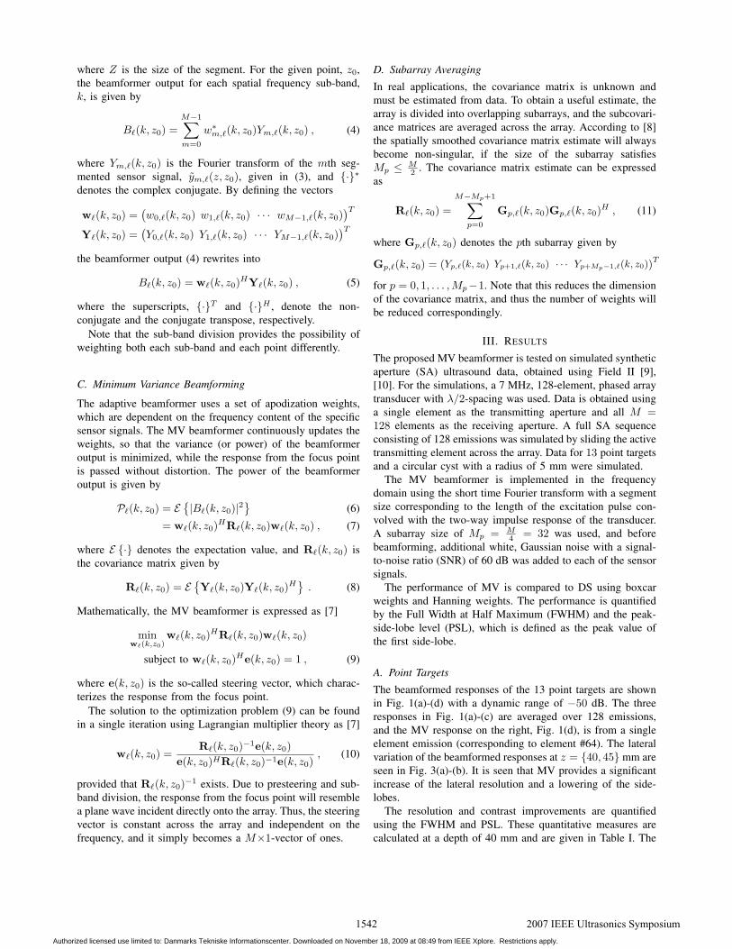
The beamformed responses of the 13 point targets are shownin Fig. 1(a)-(d) with a dynamic range of −50 dB. The threeresponses in Fig. 1(a)-(c) are averaged over 128 emissions,and the MV response on the right, Fig. 1(d), is from a singleelement emission (corresponding to element #64). The lateralvariation of the beamformed responses at z = {40, 45} mm areseen in Fig. 3(a)-(b). It is seen that MV provides a significantincrease of the lateral resolution and a lowering of the side-lobes.
The resolution and contrast improvements are quantifiedusing the FWHM and PSL. These quantitative measures arecalculated at a depth of 40 mm and are given in Table I. The
2007 IEEE Ultrasonics Symposium1542
Authorized licensed use limited to: Danmarks Tekniske Informationscenter. Downloaded on November 18, 2009 at 08:49 from IEEE Xplore. Restrictions apply.
Lateral distance [mm]
Axi
al d
ista
nce
[mm
]
−10 0 10
25
30
35
40
45
50
55
60
65
(a) DS, Boxcar
Lateral distance [mm]
Axi
al d
ista
nce
[mm
]
−10 0 10
25
30
35
40
45
50
55
60
65
(b) DS, Hanning
Lateral distance [mm]
Axi
al d
ista
nce
[mm
]
−10 0 10
25
30
35
40
45
50
55
60
65
(c) MV
Lateral distance [mm]
Axi
al d
ista
nce
[mm
]
−10 0 10
25
30
35
40
45
50
55
60
65
(d) MV, single element
Fig. 1. Beamformed responses of the 13 point targets. (a)-(c) The images are averaged over 128 emissions. (d) No averaging is applied, response from asingle element emission (element #64). All images are shown with a dynamic range of −50 dB.
measures are given for the single element emission and for thefull SA sequence. It is seen that the MV beamformer providesa significant improvement in terms of both FWHM and PSL.The FWHM of MV from a single emission response compriseonly {12.7%, 8.2%} of the FWHM from the full DS sequenceusing DS{Boxcar,Hanning}.
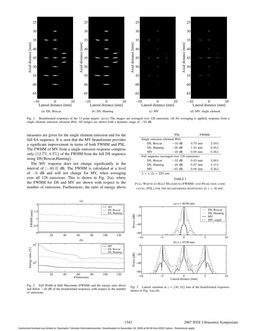
The MV response does not change significantly in theinterval of [−40; 0] dB. The FWHM is calculated at a levelof −6 dB and will not change for MV, when averagingover all 128 emissions. This is shown in Fig. 2(a), wherethe FWHM for DS and MV are shown with respect to thenumber of emissions. Furthermore, the ratio of energy above
20 40 60 80 100 1200
0.5
1
1.5
2
FWH
M [
mm
]
(a)
MVDS, BoxcarDS, Hanning
20 40 60 80 100 120
100
102
# Emissions
Ene
rgy
ratio
[%
]
(b)
MVDS, BoxcarDS, Hanning
Fig. 2. Full Width at Half Maximum (FWHM) and the energy ratio aboveand below −40 dB of the beamformed responses with respect to the numberof emissions.
PSL FWHM
Single emission (element #64)DS, Boxcar −16 dB 0.79 mm 3.59λ
DS, Hanning −36 dB 1.33 mm 6.05λ
MV −49 dB 0.08 mm 0.36λ
Full sequence (averaged over 128 emissions)DS, Boxcar −32 dB 0.63 mm 2.86λ
DS, Hanning −49 dB 0.97 mm 4.41λ
MV −65 dB 0.08 mm 0.36λ
λ = c/f0 = 220 µm
TABLE I
FULL WIDTH AT HALF MAXIMUM (FWHM) AND PEAK-SIDE-LOBE
LEVEL (PSL) FOR THE BEAMFORMED RESPONSES AT z = 40 MM.
−10 −5 0 5 10
−60
−40
−20
0
Pow
er [
dB]
(a) z = 40.00 mm
DS, BoxcarDS, HanningMVMV, single
−10 −5 0 5 10
−60
−40
−20
0
Lateral distance [mm]
Pow
er [
dB]
(b) z = 45.00 mm
Fig. 3. Lateral variation at z = {40, 45} mm of the beamformed responsesshown in Fig. 1(a)-(d).
2007 IEEE Ultrasonics Symposium1543
Authorized licensed use limited to: Danmarks Tekniske Informationscenter. Downloaded on November 18, 2009 at 08:49 from IEEE Xplore. Restrictions apply.
Lateral distance [mm]
Axi
al d
ista
nce
[mm
]
−10 −5 0 5 10
30
35
40
45
50
(a) DS, Boxcar Contrast: −18 dB
Lateral distance [mm]
Axi
al d
ista
nce
[mm
]
−10 −5 0 5 10
30
35
40
45
50
(b) DS, Hanning Contrast: −37 dB
Lateral distance [mm]
Axi
al d
ista
nce
[mm
]
−10 −5 0 5 10
30
35
40
45
50
(c) MV Contrast: −40 dB
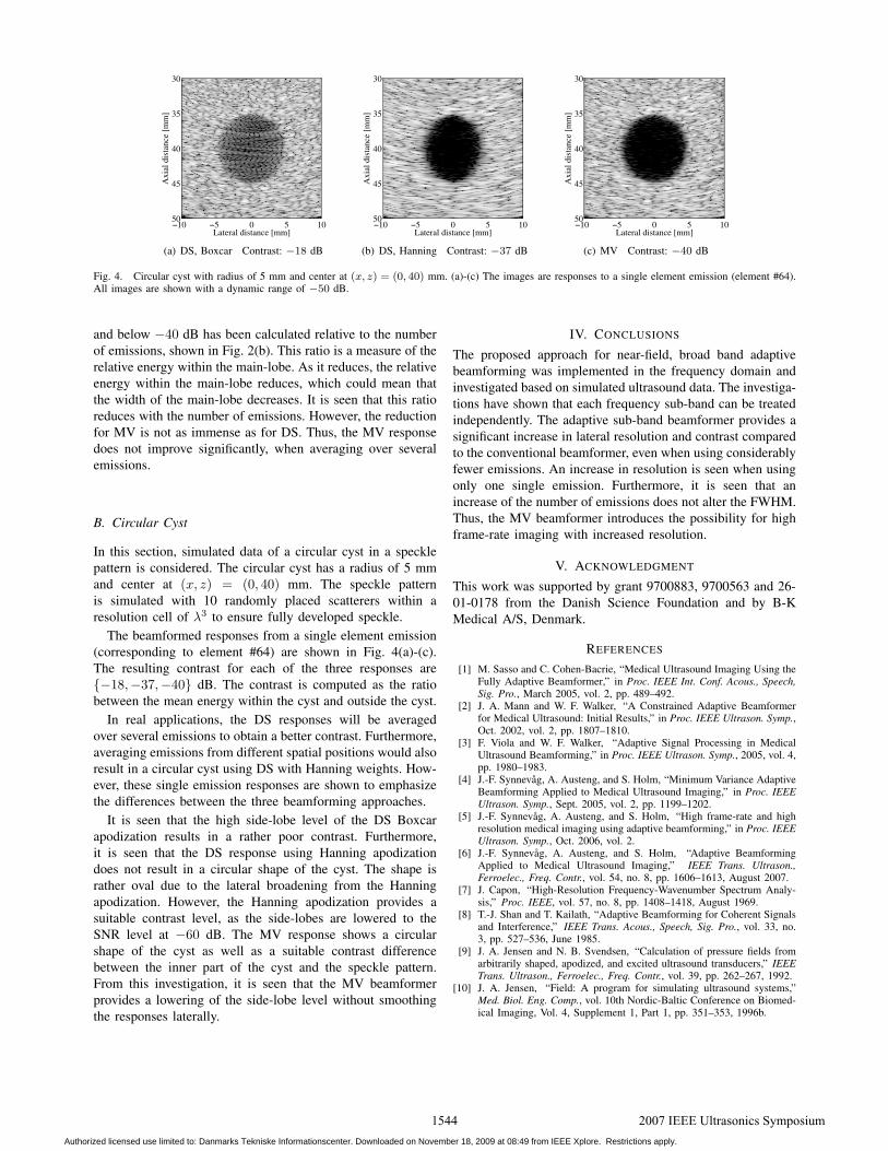
Fig. 4. Circular cyst with radius of 5 mm and center at (x, z) = (0, 40) mm. (a)-(c) The images are responses to a single element emission (element #64).All images are shown with a dynamic range of −50 dB.
and below −40 dB has been calculated relative to the numberof emissions, shown in Fig. 2(b). This ratio is a measure of therelative energy within the main-lobe. As it reduces, the relativeenergy within the main-lobe reduces, which could mean thatthe width of the main-lobe decreases. It is seen that this ratioreduces with the number of emissions. However, the reductionfor MV is not as immense as for DS. Thus, the MV responsedoes not improve significantly, when averaging over severalemissions.
B. Circular Cyst
In this section, simulated data of a circular cyst in a specklepattern is considered. The circular cyst has a radius of 5 mmand center at (x, z) = (0, 40) mm. The speckle patternis simulated with 10 randomly placed scatterers within aresolution cell of λ3 to ensure fully developed speckle.
The beamformed responses from a single element emission(corresponding to element #64) are shown in Fig. 4(a)-(c).The resulting contrast for each of the three responses are{−18,−37,−40} dB. The contrast is computed as the ratiobetween the mean energy within the cyst and outside the cyst.
In real applications, the DS responses will be averagedover several emissions to obtain a better contrast. Furthermore,averaging emissions from different spatial positions would alsoresult in a circular cyst using DS with Hanning weights. How-ever, these single emission responses are shown to emphasizethe differences between the three beamforming approaches.
It is seen that the high side-lobe level of the DS Boxcarapodization results in a rather poor contrast. Furthermore,it is seen that the DS response using Hanning apodizationdoes not result in a circular shape of the cyst. The shape israther oval due to the lateral broadening from the Hanningapodization. However, the Hanning apodization provides asuitable contrast level, as the side-lobes are lowered to theSNR level at −60 dB. The MV response shows a circularshape of the cyst as well as a suitable contrast differencebetween the inner part of the cyst and the speckle pattern.From this investigation, it is seen that the MV beamformerprovides a lowering of the side-lobe level without smoothingthe responses laterally.
IV. CONCLUSIONS
The proposed approach for near-field, broad band adaptivebeamforming was implemented in the frequency domain andinvestigated based on simulated ultrasound data. The investiga-tions have shown that each frequency sub-band can be treatedindependently. The adaptive sub-band beamformer provides asignificant increase in lateral resolution and contrast comparedto the conventional beamformer, even when using considerablyfewer emissions. An increase in resolution is seen when usingonly one single emission. Furthermore, it is seen that anincrease of the number of emissions does not alter the FWHM.Thus, the MV beamformer introduces the possibility for highframe-rate imaging with increased resolution.
V. ACKNOWLEDGMENT
This work was supported by grant 9700883, 9700563 and 26-01-0178 from the Danish Science Foundation and by B-KMedical A/S, Denmark.
REFERENCES
[1] M. Sasso and C. Cohen-Bacrie, “Medical Ultrasound Imaging Using theFully Adaptive Beamformer,” in Proc. IEEE Int. Conf. Acous., Speech,Sig. Pro., March 2005, vol. 2, pp. 489–492.
[2] J. A. Mann and W. F. Walker, “A Constrained Adaptive Beamformerfor Medical Ultrasound: Initial Results,” in Proc. IEEE Ultrason. Symp.,Oct. 2002, vol. 2, pp. 1807–1810.
[3] F. Viola and W. F. Walker, “Adaptive Signal Processing in MedicalUltrasound Beamforming,” in Proc. IEEE Ultrason. Symp., 2005, vol. 4,pp. 1980–1983.
[4] J.-F. Synnevag, A. Austeng, and S. Holm, “Minimum Variance AdaptiveBeamforming Applied to Medical Ultrasound Imaging,” in Proc. IEEEUltrason. Symp., Sept. 2005, vol. 2, pp. 1199–1202.
[5] J.-F. Synnevag, A. Austeng, and S. Holm, “High frame-rate and highresolution medical imaging using adaptive beamforming,” in Proc. IEEEUltrason. Symp., Oct. 2006, vol. 2.
[6] J.-F. Synnevag, A. Austeng, and S. Holm, “Adaptive BeamformingApplied to Medical Ultrasound Imaging,” IEEE Trans. Ultrason.,Ferroelec., Freq. Contr., vol. 54, no. 8, pp. 1606–1613, August 2007.
[7] J. Capon, “High-Resolution Frequency-Wavenumber Spectrum Analy-sis,” Proc. IEEE, vol. 57, no. 8, pp. 1408–1418, August 1969.
[8] T.-J. Shan and T. Kailath, “Adaptive Beamforming for Coherent Signalsand Interference,” IEEE Trans. Acous., Speech, Sig. Pro., vol. 33, no.3, pp. 527–536, June 1985.
[9] J. A. Jensen and N. B. Svendsen, “Calculation of pressure fields fromarbitrarily shaped, apodized, and excited ultrasound transducers,” IEEETrans. Ultrason., Ferroelec., Freq. Contr., vol. 39, pp. 262–267, 1992.
[10] J. A. Jensen, “Field: A program for simulating ultrasound systems,”Med. Biol. Eng. Comp., vol. 10th Nordic-Baltic Conference on Biomed-ical Imaging, Vol. 4, Supplement 1, Part 1, pp. 351–353, 1996b.
2007 IEEE Ultrasonics Symposium1544
Authorized licensed use limited to: Danmarks Tekniske Informationscenter. Downloaded on November 18, 2009 at 08:49 from IEEE Xplore. Restrictions apply.