AD-R163 231 THE P-VERSION OF THE FINITE ELEMENT METHOD FOR vi'CONSTRAINT BOUNDARY CONDIT..(U) MARYLAND UNIV COLLEGEPARK INST FOR PHYSICAL SCIENCE AND TECH.

UNCLASSIFIED I RUSKA ETAL. APR 87 N-i96F/G 22

mhmmhhhmhhhhuEu'."osmmm

111.0 1" 18 N

1.2111111. '

MICROCOPY RESOLUTION TEST CHARTNATIONAL BUREAU OF STANDARDS-1963-A

11111mr

w 7W:~w~ - ~iW~ 'w -~ -~ . -

bmi REM

I FILE COPy

MARYLAND S ECTE

COLLEGE PARK CAMPUS

The p-version of the finite element method

cv for constraint boundary conditions

I. Babu.gka00 Institute for Physical Science and Technology

University of MarylandCollege Park, Maryland 20T42

Iand

Manil SuriDepartmerk of Mathematics

University of Mayland Baltimore CountyCatonsville,-Maryland 21228

Technical Note BN-1064

DESTRIBTION STATZ I"dE AApproved for public reloase:

Dbtlibufm Uniadd April 1987

INSTITUTE P:OR PI-IYSICAL SCI:NCC=AND TQC CINOLOOY

87 7 29 004

Lnci u.)

SECUP11TV CLASSUICATION OF THI PAGE (3Mma Do*mw _______________

1. ISPRT umeft6. RCPORMN CAORG ENRUMER

7. AUTNOR1(s) L. CONTRAT Olt G*AXT HUMNEW'u

I. Babuska and Manil Suri AFOSR 85-0322

S. PERFORMNG ORGANS ZATION HNM AND ADDRSS I0. P"MM9 MI11T.4 PRJCT. TASKUnivesityof Mrylad, ColegePK, 0742Al S WOobK UNIT NUtrS

Institute for Physical Science and Technology

Department of Mathematics, UMBC, Catonsvi1 ~ ______________

It. CONTROLLING OFFICE NMN AND ADDRESS I2 REPORT OATS

Department of the Navy Apr. NU 1987PAE

Of fice of Naval Research1. Uf OPAE

14. MOWS MGr ASSN NAME £ ADDRESSj(S t.Vjmt 1m. CdPWjhV*MdQO.) IL SECURITY CLASS (of We NPWQI

1S. DISTRIIUUTION STATEMENT (of Wet Repeed)

Approved for public release: distribution unlimited

17. 'DISTRIEUTION STATEMENT (of IA. Aobe*M etod A tob 104 20 fit 600m. 1mM RpIN1

Id. SUPPLEMENTARY NOTES

Is. KEY WORDS rG..tbw.em on 0~0 aide It waom mod I I -IF by WeekA alober)

20. AUSTRACT (CemWM an mrVna0 side 11 nemea and WdSW& bP 6" Moo"ama.

The paper addresses the impleme ntation of general constraint boundaryconditions for a system of equations by the p-version of the finite elementmethod. By constraint boundary conditions we mean conditions where somerelation between the components is prescribed at the boundary. Optimal errorbounds are proven.

DO I j"' 14 73 EDITION OIP I NOV of #a GOWRLETES/N 0I102- LP. 014. 6601 UCURTV CL.ASUPICATIW OF YNIS PAGE (Whom N

The p-version of the finite element method

for constraint boundary conditions

by

1. Babuska'

Institute for Physical Science and TechnologyUniversity of Maryland

College Park, Maryland 20742

and

Manil Suri2

Department of MathematicsUniversity of Maryland Baltimore County

Catonsville, Maryland 21228

'Partially supported by ONR Contract OOO14-85-K-0169.

2 Research partially supported by the Air Force Office of Scien-tific Research, Air Force Systems Command, USAF, under Grant No.AJOSR- 65-0322.

The p-version of the finite element method

for constraint boundary conditions

Abstract. Ie paper addresses the implementation of general

constraint boundary conditions for a system of equations by the

p-version of the finite element method. By constraint boundaryfke, awl)os

conditions ke conditions where some relation between the

components is prescribed at the boundary. Optimal error bounds

are proven. 01 V4 5f

U .!AI J +,l .

r.

L' . . . .

i T:f l,J.,t-. ix

I)TIC

1. Introduction.

There Is a large variety of boundary conditions for systems

of differential equations of elliptic type. Some physically natu-

ral conditions may be formulated by a variational approach through

constrait conditions. For example, the two dimensional elastici-

ty problem can be formulated as the minimization of a quadratic

functional F(u), u - (u1 ,u2 ) over a set H satisfying

1 2 1 2(H ()) c H c (H (0))

*Selections of H then characterize the boundary conditions.

Obviously the choice H - (H (0))2 induces the (essential)

Dirichlet conditions, i.e., the displacement is given on 00,

while H - (H (0))2 induces the (natural) Neumann conditions,

i.e., the tractions are prescribed on ao. In addition to these

classical conditions other types are important in applications.

One of these conditions is characterized by

(1.1) H - ((ulu 2 )e (H())2 101 (s) + u20 2 (s) - 0 on 00)

where P1 and p2 are given functions defined on 00. These con-

ditions are in the most simple case tfe symmetry conditions and in

general traction free constraints at the boundary.

So far we have only mentioned homogeneous boundary conditions.

Nonhomogeneous conditions are defined in the usual way, when the

minimization of F is over a hyperplane H - (u + vj u c H,V

v C (H (I) 2).

The constraint boundary condition we mentioned above Is a type

of essential condition. Hence when solving such problems by the

finite element method In general and by the p or h-p versions

2

in particular, we face the problem of implementing the nonhomogen-

neous boundary conditions (which are outside the finite element

space).

The p and h-p versions are recent developments, where p,

the degree of the elements used is not fixed but is increasing.

This is in contrast to the classical h-version, where the degree

p is kept fixed. The first commercial programs available are

PROBE (Noetic Tech., St. Louis) and FIESTA (ISHES, Bergamo, Italy).

The implementation of Dirichlet boundary conditions for the

p-version of the finite element method has been addressed by us in

(2] and (4]. A general survey on the state of the art of the p

and h-p versions may be found in (1].

In this paper we will address the implementation of the con-

straint conditions (1.1) in a simplified setting (to avoid nota-

tional difficulties). Section 2 deals with preliminaries and

notation. In Section 3 we formulate an abstract approach and

based on it prove that the suggested finite element formulation of

the constraint boundary condition leads to the optimal rate of

convergence of the p-version. Section 4 addresses some imple-

mentatlonal aspects.

3

2. The basic notation and preliminaries.

2.1. The Sobolev spaces

Let P 2 be the two dimensional Euclidean space, x - (x1,x 2)

p 2 . Let 0 c P 2be a bounded Lipschitzian domain with the boun-

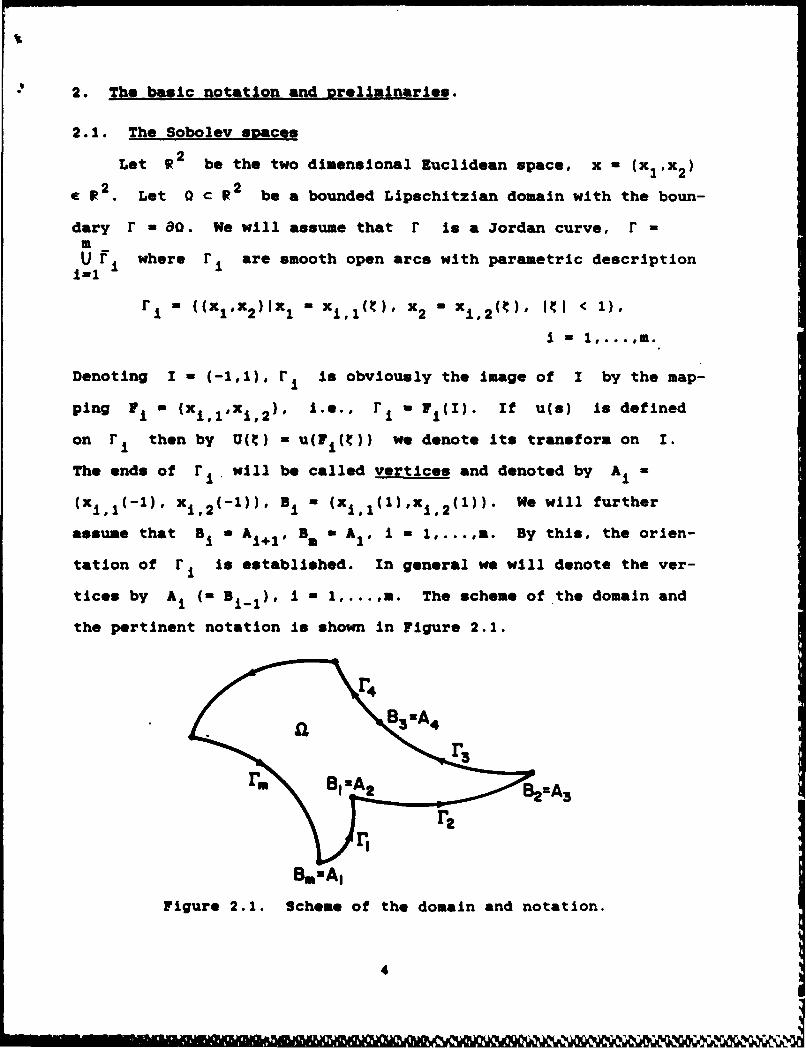
dary r - 80. We will assume that r is a Jordan curve, rm

U r I where r are smooth open arcs with parametric description

r - ((2C11x2)1x1 M X i'l(t), x 2 M- 1,2 (t) R1t < 1).

Denoting I - (-1.1), r is obviously the image of I by the map-

ping Fj - (X Il x 12' i.e., r I 1FI(I). If u(s) is defined

on rIthen by U(R) -u( i (M) we denote its transform on 1.

The ends of r I.will be called vertices and denoted by Ai I

(x iil(-l), xi12(-1)). , B (X1 I'(l).x 12 (1)). We will further

assume that B I= iA i+1 Bma - Ale i - le ...on. By this, the orien-

tation of r IIs established. In general we will denote the ver-

tices by A I (M B i-1)# I -1 .m The scheme of the domain and

the pertinent notation Is shown In Figure 2.1.

r4

Remark 2.1. We assumed that the domain Q is simply connected.

This assumption has been made only for notational simplicity.

Remark 2.2. We assumed that the domain is Lipschitzian. Once

more, our results are valid (with proper modification) in the case

when, for example, some arcs coincide (as in the case of the slit

domain).

Remark 2.3. We have assumed that the arcs F are sufficiently

smooth. For the sake of simplicity we assume that they are Cm

arcs (i.e., the functions x ij , i = 1, ...,m, J = 1,2 are C'm

functions).

By H k(Q), k a 0 integer we denote the usual Sobolev space

of functions with square integrable derivatives on 0. The norm

will be denoted by k!*I~ . If t < q <.t+l, t 0 integer,

then we define Hq(Q) - (Ht(O),Ht+1 ()) 0 , 0 = q-t where by

we denote the usual Interpolated space using the K-method

(see (5]). The scalar product (.,.) and the norm Hq.(0

are defined accordingly.

By C (5), k z 0 integer, we denote the space of all func-

tions with k continuous derivatives on Q. It is possible toIcIshow that H (0) '-p C0( M for k > 1, where by L-. we denote

continuous imbedding. On the other hand, H1(0) 4 C0 (6).

For I - (-1,1), H k(I), k z 0 is defined analogously as

before. If k > 1/2 then H k(I) - C0 (I) but Hk(I) a C0(I)

for k s 1/2.

So far we have defined H k(I), k a 0. We will also be inter-

ested in H k(I), < 0. We define for k i 0

5

• o'I

s uvdx

-1kH-k (I} vO V1Hk (1)

(Let us remark that sometimes (see e.g. (5]) our space H-k(I) is

denoted by (H ())' whereas H-k (I) is used to denote the dual

space of Hk()).

If u is defined on r then we define

H k(y) = {uju(F1 (9)) - U(t) - H k(I))

11 uli = ! u I.Hq(r H k (I)

So far we have considered only scalar functions on Q and I.

The spaces of vector functions are defined by Cartesian products,

2H k(0) (H k(o)) 2 .

Let now

Q = ((x,*X2)11x 11 < 1, Ix21 < 1)

= ((x1 ,x2)11x I < 1, x -1)

Q will be called the standard square and rQ, 1 - 1,2,3,4 Its

sides ({Q, i - 2,3,4 are defined analogously to rQ in an

obvious way). Let

T - ((x,x2)11x1 1 < 1, 0 < x2 < (1+x1) for x < 0,

0 < x2 < (1-xI)/I1 for x > 0)

T - (IXM 1<1 )1 (xx 2) 1* 2 )

TT will be called the standard triangle and r1 i - 1.2,3 its

sides.

6

- - :.~e'~'

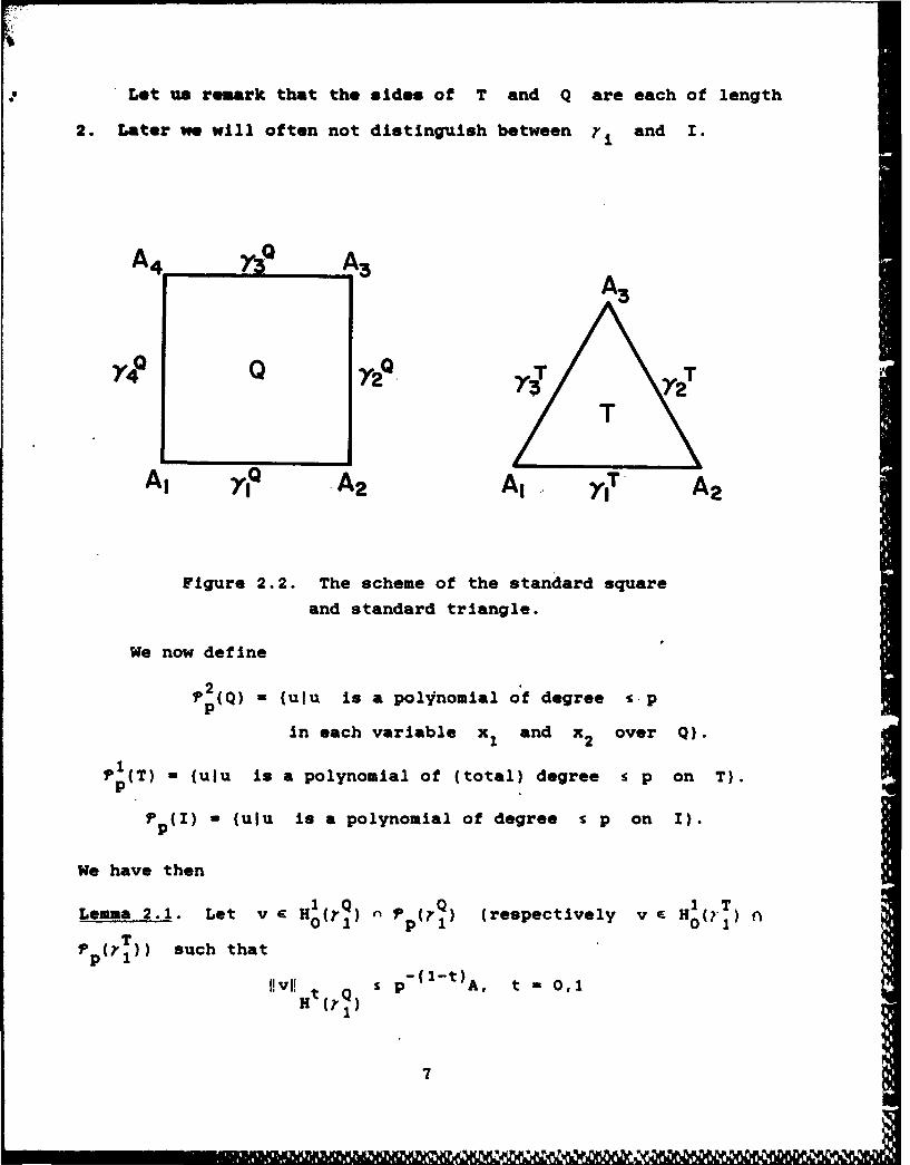
'U Lot us remark that the sides of T and Q are each of length

2. Later we will often not distinguish between r .and 1.

A4_______ 3 A3

Y4 QT T

T

Al A2 Al 7 T- A2

Figure 2.2. The scheme of the standard square

and standard triangle.

We now define

P? (Q) - (ulu is a polynomial of degree %-pp

In each variable x 1 and overover

P()- (ulu is a polynomial of (total) degree s p on T).p

P p(1) - (ulu is a polynomial of degree Sp on I).

We have then

Lemma 2.1. Let v e H Qr) "P (rQ (respectively v e 1( T)0 1 p1 H0 (r 1)P (r T such that

HvB! t Q p- ( 1t)A, t - 0,1

7

* respectively

T vl p ltA, t =0,1.

H (V1)

Then there exists u e 2 (Q) (respectively P1 (T)) such thatp p

ul IV = v (respectively uj I T =V), ul CI- 0 (respectively

uj T- T = 0) andT-1

Pul 1 5 C-1/2A

respectively

fHui I Cp 1 / 'A.

For the proof see (2] or [3].

2.2. The model problem

Let

2H 1(0) c Xt(Q) c 2H 1 (Q)0

where X(Q) Is closed in 2H 1(0). X(Q) will be called the con-

straint space. Assume that there is given a continuous bilinear

form B(u,v) on 2 H I (Q) - ~H I(0),.u = (u11u ), v = (v11v') such

tha t

(2.1) .B(u,u) a vllul;,2 Y > 0 for any u e 2 H 1 (0).2H1 (0)

Then obviously for any G1 -E (X(O))', there is a unique u0 S t0

such that

B(u01 v) = G 1 (v)

holds for any v X (Q). We also have

U 0 2H I ( Q) 'S C ! ( H 1 ( 0 ) ) ,

Denote X (0) = (U 2 H (0), u-p C X(Q)). x (0) will bep p

called the p-hyperplane. Then our model problem is given by:

Find u 0 e P (0) such that

(2.2) B(uoV) = G1 (v), V v E X(Q).

We have then

(2.3) :u0 !2 1 C[IPH! 1 + G 1 !! 2 1.H() H(0) 1H H())

If p = 0 then we will speak about a homogeneous constraint

problem while for p * 0 we will speak about a nonhomogeneous

constraint problem. We call these constraint problems because

I(Q) - 2HI(Q)

There are many constraint problems in applications. We will

consider the one when

.2

X(Q) = ((u11u) 2 H 1(Q)I Zc~$) ue~ 0, k = 1,2, j=t=i

where a = {0 are matrices of smooth functions on r (say

C OD )) Additional assumptions on (k,)p will be imposed

later.

Obviously when ak,k = , k, 0 for k # t we get Dirn-

chlet boundary conditions (in general we get Dirichlet conditions

when a have rank 2 for all x e r ) If (ak = 0 there

is no constraint and we have the Neumann problem.

If aJ has rank 1 then we can write the constraint on r

as

0()u1 + a0 u =01111 1,2 2

which will be written in the form

9

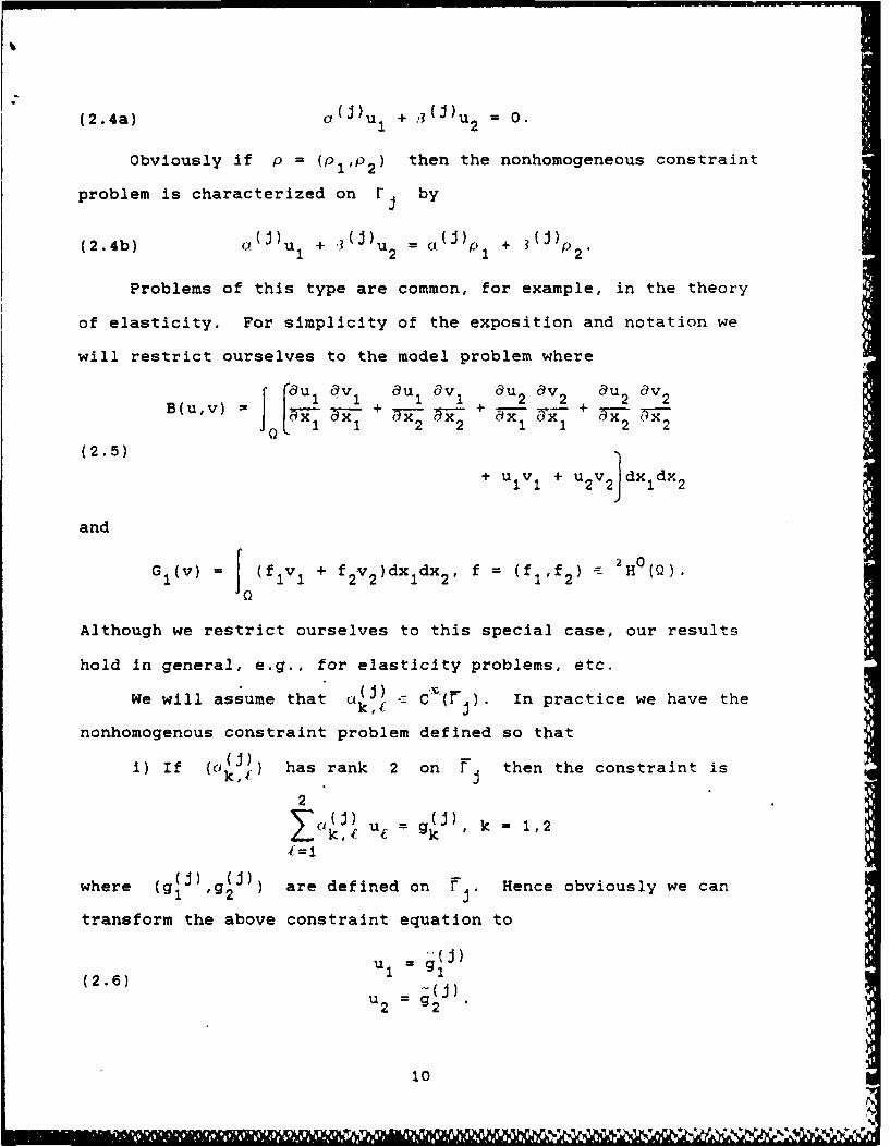
(2.4a) a(J)u + ,3(u 2 = 0.

Obviously if p = (p1 ,P2 ) then the nonhomogeneous constraint

problem is characterized on r by

(2.4b) A ,(J)U I + 3 (J)u2 = C1 U p1 + 3(j)

Problems of this type are common, for example, in the theory

of elasticity. For simplicity of the exposition and notation we

will restrict ourselves to the model problem where

B(u,v) = au 1V 1 u3 1 + au xa 2 + aux2 av2

[JQ, -,i 1 '7X2 7x2 1 1 2 7x2(2.5) 9

+ U1V1 + u2v2 dxldx2

and

00G 1(V) = (f IV I + f 2 v 2)dX IdX 2F f = (flif 2) H 2H(Q).

Although we restrict ourselves to this special case, our results

hold in general, e.g., for elasticity problems, etc.

We will assume that (j) C".(r. In practice we have the

nonhomogenous constraint problem defined so that{ (J)

i) If (ok,4 has rank 2 on F then the constraint is

2

(4=1c )Uk , = g (), k = 1,2

where (g1) ,g2)) are defined on r-J, Hence obviously we can

transform the above constraint equation to

(2.6) 1 "I)u 2 g2

10

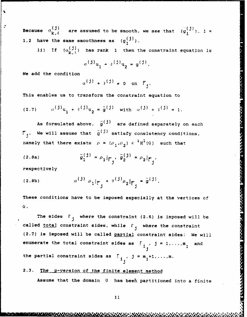
B au e ((J ) '(J)Because are assumed to be smooth, we see that (g9 }, 1 =

1,2 have the same smoothness as (glj)}.

( (j)ii) If (c}k,t has rank 1 then the constraint equation is

0(j)U 1 +3(J)u 2 =g(J)

We add the condition

a(J ) + 3(j) o 0 on Fa.

This enables us to transform the constraint equation to

(2.7) !(J)U I + 3(j)U 2 = g(J) with U(j ) + 3(j) = 1.

As formulated above, g are defined separately on each

rJ. We will assume that g(j) satisfy consistency conditions,

namely that there exists p = (p1,P2 ) 2H 1(Q) such that

(2.8a) iJ) = P= p2J- -1g 1 1 F- g2 21F

respectively

(2.8b) 0(J) Pr i+ 3(j) P 2 1F =g

These conditions have to be imposed especially at the vertices cf

The sides r where the constraint (2.6) is imposed will bea€

called total constraint sides, while F where the constraint

(2.7) is imposed will be called partial constraint sides: We will

enumerate the total constraint sides as i JF j = 1,...,m and

the partial constraint sides as rIJ, j = m +1,...,m.

2.3. The p-version of the finite element method

Assume that the domain Q has beeh partitioned into a f-inite

11

p.

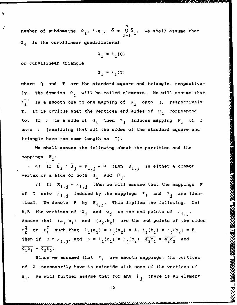
nnumber of subdomains 01, i.e., 0 = U 0 We shall assume thati=1I

Q is the curvilinear quadrilateral

o =i(Q )

or curvilinear triangle

0 =i(T)

where Q and T are the standard square and triangle, respective-

ly. The domains 0 will be called elements. We will assume that

T-I is a smooth one to one mapping of 0 onto Q, respectively

T. It is obvious what the vertices and sides of Q4 correspond

to. If / is a side of 0 then 7 induces mapping Fi of I

onto I (realizing that all the sides of the standard square and

triangle have the same length as I).

We shall assume the following about the partition and the

mappings F :

. 0) If I - 0 = Rij -0 then R,,j is either a common

vertex or a side of both 0 and 0 J

3) If Ri'j = 7i,j then we will assume that the mappings F

of I onto ?,j induced by the mappings Vi and w are iden-

tical. We denote F by Fij. This implies the following. Let

A,B the vertices-of O0 and 0 be the end points of

Assume that (al,b 1 ) and (a2,b2 ) are the end points of the sides

'k or T such that (a = j(a2) = A, 7 (b1 ) = %(b 2 ) = B.

Then if C e )i,j, and C i j(c 1 ) =7 1 (c2 ), a1c= a2c= and

b= =1 1 2 2

Since we assumed that I are smooth mappings, the vertices

of 0 necessarily have tc coincide with some of the vertices of

Q We will further assume that for any F there is an element

12

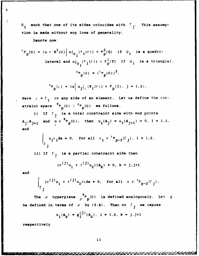
o such that one of its sides coincides with rJ This assump-

tion is made without any loss of generality.

Denote now

( (0 ( = 1 ) u P 2(Q) if 0 is a quadri-HpO -( lQ uIQoi( t p 1

lateral and ujl (T 101)) -- ? 1(T) if 0 is a triangle),i pi

1p (0) - (?P (0)) 2

2. , ) = {(U} UjI (FI (t P p( ), 1,2).

Here j = r or any side of an element. Let us define the con-

straint space r (0) z 2p (0) as follows.p p

i) If P is a total constraint side with end points

AJ0A J+1 and u EVP p(0), then u I(A = ui(Aj+i 1 = 0, i = 1,2,

and

[ uitids - O, for all 1- 2 (r ) i = 1,2.P

ii) If P is a partial constraint side then

(0(J)u 1+ ,3(J)u2 )(Ak) 0 0, k - JJ+1

and

1 (Uj)u 2 + (J 1u2 )ds - 0, for all r 2Ira

The p hyperplane Q p(Q) is defined analogously. Let g

be defined in terms of p by (2.8). Then on r we impose

ui(Ak) = g i)(ak), i = 1,2, Ic J,J+1

respectively

13

((J) ~u 1 + !(J) 2 HA k) - g W(k .- ,+

and

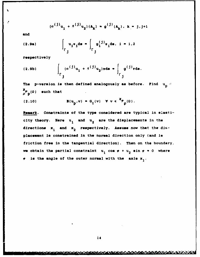
(2.9a) g o- 9 1 P 'do, I - 1,2Ir u1 1 s

respectively

(2.9b) fr (Oa~ 'I + #3(J) u2 )Yds - fr 1 rs

The p-version ithndefined anlgul sbefore. Find u -

P(0) such thatPp

(2.10) B(u 'v) -G (v) Vv C P (0).p p

Remark. Constraints of the type considered are typical In elasti-

city theory. Here u1and u 2 are the displacements In the

directions x1and x 2 respectively. Assume now that the dis-

placement is constrained In the normal direction only (and Is

friction free in the tangential direction). Then on the boundary,

we obtain the partial constraint u I coon 0 + u 2 sin f a 0 where

v is the angle of the outer normal with the axis x I'

14

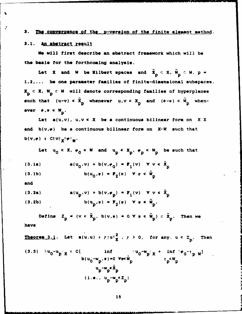
S. Th cveraence of the p-verson of the finite element method.

3. 1. An abstra _"eWsult

We will first describe an abstract framework which will be

the basis for the forthcoming analysis.

Lot X and W be Hilbert spaces and Xp C X, Wp W, p

1.2.... be one parameter families of finite-dimensional subspaces.

xp C X. N p W will denote corresponding families of hyperplanes

such that (u-v) e Xp whenever u,v E Xp and (O-v) e Wp when-

ever ,ve N Vp.

Let a(u,v), u,v e X be a continuous bilinear form on X X

and b(v,v) be a continuous bilinear form on X-W such that

b(v,*) % CI!vP x M;!.

Let u0 e X, 0 0 W and u p Xp, p 4 W p be such that

(3.1a) a(uov) + b(v, O0 ) = (v) V v C p

(3.1b) b(uoV) - VF2 () V r C Wp

and

(3.2a) a(upv) + b(VVp F(v) V v C Xp

(3.2b) b(u p W) - 2() V 0 C p.

Define Zp W (V C Xp, b(v,*) - 0 V V Wp) C X P. Then we

have

2Theor a 3. Let a(u,u) r r!u,: , > 0, for any. u c Z . Then

(3.3) !iuoU s Cc nf ;,uowp + tnf O-p W]

b(uo-Wp , I) 0 Vp Wp l EWp

(i.e., u p-WE Zp)

15

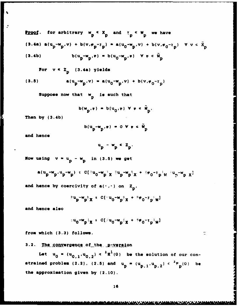
troo. for arbitrary w p cX arnd t p W pwe have

(3.4a) a(u,-wp DV) * b~vop, - a(u0 -w ,v) + b~~ox) V v i X

(3.4b) b(u -w~ p P) - b(u 0 -W Y) V r' p

For v a Z (3.4a) yields

(3.5) a(u -w p .v) - a(u 0 -W v) + bvV0

Suppose now that w pis such that

b(w p r) - b(u0 OV) V 0 p W

Then by (3.4b)

b(u p-W pP) - 0 V 0 p

and hence

now using v-up w. in (3.5) we got

a(u -w ,u -w ) C(Iu -wp ~ 'u -W1i+' _p p p p 0 p I p p .X 09~' p UIn x1

and hence by coercivity of a(-,-) on Z p

"1u -w + H C40- '1p p!X S C - p ! 0 ,p..

and hence also

U w I C (,;u pX + 1! o ;pIW

fram which (3.3) follows.

3.2. The onergqpqA of the__V-yerpJon

Let u (U 0 11 ,u 0) H I(Q) be the solution of our con-

strained problem (2.2), (2.5) and up M (u 'IU p 2) 1P (0) be

the approximation given by (2.10).

----------

9"

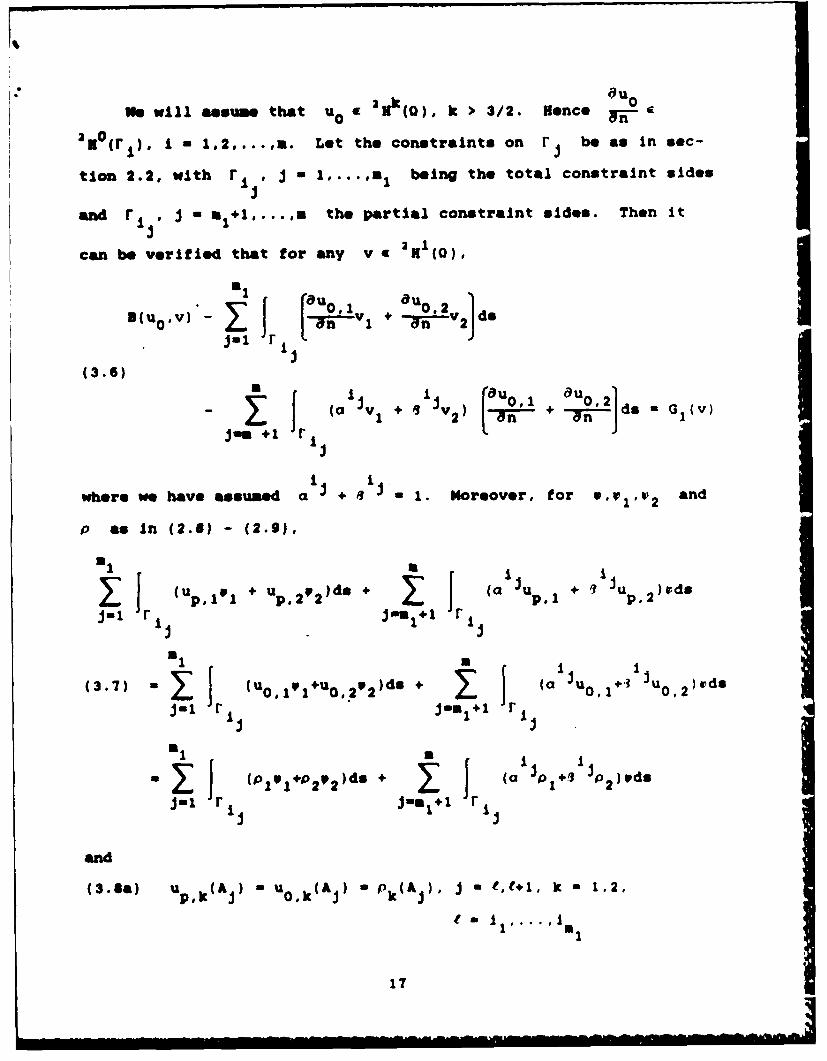
We will assume that u 41 20X(0), k > 3/2. Hence 00 87-

2 0(rL) I - 1,2,.... Let the constraints on r be as in sec-

tion 2.2, with r , J l.an being the total constraint sides

and r I J, J a 1 ..., the partial constraint sides. Then it

can be verified that for any v a aH (0),

B~ JV) 0 u 2 ) doJ-1 r nOI vI+d

(3.6)

(a 5 1 2) ( +- -ya' -Jdo - G(v)

where we have assumed a + '3 = 1. Moreover, for P.Plp 2 and

p as in (2.0) - (2.9),

(Up + 1 V )p2 2 do + (a Up, 1 + I i u ,2 rd

SrJI

(3.7) = (uO +U V )do + (a1JUO'+' 1 JUo 2lds

mml JI i i

- . (p 9 +4P2 2 )do + (a ' 1 +3 Jp )wds

J- ri J- m 1+1 r _

and

(3.1a) up,klAj) A uoklA3 ) ( pk(AJ), t , 4,1, k - 1.2,

, l.....

1 a1

17

(a Up P'I)(A ) J +(0 uV,2 )(A ) - (aU 0,1)(HA) + (3tuO0,2)(A )

(3.8b) - 01 (2 HA 0 0 02 )(Aj

JeJ- e,e+1, C - ti+ ... is

(O remark that u 0 '1 (At), I - 1,2 has meaning because we assumed

that u0 aflk(Q), k > 3/2).

We now define

X * 21I(0), di.i =I.,

H (0)

and for any 6 - (61,62) C X,

Xp. 6 a- (U (u 2) app(), uk(AJ) - 6k(AJ) k - 1,2

I 1 2

- -aI .)(A ) * 5 A .... C -+ (, )(1Aa).

We then take in our abstract framework

Xp - Xp, , Xp - Xp.O

where p satisfies (2.6) - (2.6). Moreover, lot

fl H 1/2( a- 1/2l a.,

with the norm

al m 1/2

[u [ZN- /2(r I Jn 1 + H (r

O see then that o q N whore (see (3.6))

is

Au1 0,2 i

' j = - 0- - I r 41 n --r 1 1. ,. . m

n k ], J M 1 ..M

Define W p p W jWp c W where

IWp ) H_12( 2e P1- (

I H-1 / 2 (rl ) p_ 2 (r), a - +l1 ...p. . -

Let a(-.-) and b(,*) be bilinear forms defined respec-

tively on XX and K-N by

a(u,v) - B(u,v)

b(u,p) 1 10i 1 + U202 )do + (a 1 uI + 3 1 J )v de.Jr i Ja1+1 r i

It may be seen that the right hand side of (3.7) defines a linearfunctional G2 on W . Then (3.6) - (3.8) show that (u0 #00 )

satisfy (3.1) with F k - 1,2. Moreover, if we can find a

unique pair (u p. ) satisfying (3.2), then up will be precise-

ly our finite element solution satisfying (2.10). We will now

verify that the mixed method defined above satisfies the assump-

tions of Theorem 3.1. This in turn will lead to the existence and

uniqueness of the solution (U p0 p of (3.2) and an estimate of

the rate of convergence of up to u.

Obviously, a(uv) satisfies the desired continuity and

19

coercivity conditions. for j a 1,2,...,n we have

1rue doIS C H~ 1/2(r ) k -12(

from which the continuity of b(-,) may be deduced. Hence

Theorem 3.1 is applicable. Let us now estimate inf 0- fWr-EW

p

k-3/2(First, let m 1+1 s j m. We assumed that 0ojr H I(F. ), k >

3/2. Hence o Oj (F i +) H k-3/2 (I). Let (Y p-2j (I.

be such that

J39)a d& # P d4., V P p-2 MI .

Then, with q= - a, we have

( 3 .1 0 ) q H 0 ( ) C p ( k 3 / 2 ) H - / 2 ( )

Now, for arbitrary v EH 1I (I), we have by (3.9)

J qv d? j q(v-a 1)dt q H0 ()V-(71 H0(1 P1

v 1 -W1 H(I)1 H0 1H (I) H (I) 1 H(I)

where a1 is a polynomial of degree p - 2 satisfying

.v -a1 0 Cp -v 1 I*This yields

(3.11) q H 1 (1 P (~k 1/2). + k-3/2 ( )

Interpolating (3.10), (3.11) and using the fact that F is a

smooth mapping, we obtain 2

20-m t j1

inf 1,1 -x01 1 (1/2 Cp ~ Oij !k-3/2(

We get similar estimates for r = 1J. .. m, so that

(3.12) mtf 110 - P ! :5Cp 0(ic2.zP MW PH()

We now estimate inf :u 0 - w !Ix, Using the results from [2], there

exist z P (0), 1 = 1,2 such that

(3. 3a !! O i- I I t(Q) :5 C -( - )I , !H k(0), 1 = ,2 t = 0 1

(3.13b) U 0i1(N) = z i(N) for each node N of the mesh

(3.13c) Iu 0 -z I' !! Htr SCp(k1/2t) P 0i kI (0,t =0,1, 1 = 1,2

Let ma +1 s j sa. Let us denote x = a JuO,-I)+31Ju02z2)

Then we have x(A i - r (A ) +1 0. Let m(k) - x(F( )) and let

T(F(k)) 'P P()~~ (1) Satisfy T(±l) - 0 and

v dk ;v d, V~ve 'Pp-2(i

Because of (3.13b) we can write

J ''dt dr,, V P P(1), (,)±1) = 0

and hence by Lemma 3.2 of (2]

!! -;; H(I)1/-) l 0 V2 k( t=0)

Using (3.13c), this gives

21

H t(1) 0H kQ

Now using Lemma 2.1 it follows that there is a w e I P (0) such

that w =0 on Q - where 0 is the element with the side

r W=T on r w=0 on a6 -r and

(3.14) !iw!! S Cp k-1) Iu 0 !U

Letting w =(w,w) H 1(0), we see that w will satis-ii ii

fy (3.14) with H (0) replaced by H 1(0).

Let now w = z + w i i zFZ2+ (w,w). Using (3.13b) and

the fact that w(A.) =0, we obtain

(a i (u lw)' + 0 (u 0 2 w p 2 ))(Ae) = 0, t = J I~ i +1.

Moreover, for v e P p-2 (r~ )

Iri a Ju 11w 'l+ J 0 ,2 W p2 ))vp ds

Jr (K - (a + (3 1 w)v ds = Iri(x-w)V, ds = 0

where we have used a a+0 a 1. We may construct wi as

above for all partial constraint sides. An analogous construction

can be carried out for total constraint sides as well. Then if

m

we see that

22

u - w IEXp p p

b (uo-W, ) = 0, V , W0 p p

andm

Up ,, +__ p 5 w1u <Cp-(k-l)du! 2 kJ=1 H (

This provides a bound for the first term in the right hand side of

(3.3). Hence we have proven

Theorem 3.2. Let 2H k(Q), k > 3/2. Then

;1u - ! < Cp- (k-1),juCp ' 210 2kHH () (Q)

where u0 is the exact solution and up is the finite element

solution of the constrained problem, provided that u0 and up

exist .o

The next theorem deals with the question of existence and

uniqueness of (u0 1 O) and (u ,p ).

Theorem 3.3. The (exact) solution (uol O) of the constrained

problem exists. The finite element solution (U p.P ) exists and

is unique.

Proof. In Section 2.2 we have shown that u0 exists and hence

(Uo,1o) exists, too. The finite element solution (U p, p) is

determined by the solution of a linear system of equations with

square matrix. Hence the existence follows from the uniqueness. -

Assume therefore that there is a solution (u ,pp ) of the trivial

problem. Obviously u = = 0 is also a solution of this problem.

Hence u = 0 because of Theorem 3.1. We have to show thereforep

that

23

r v + 3?v2) p d = 0

I

implies Vp 0. Because a + 3 = 1 we also have v' dP = 011

for all v 1 (1 n H0 (I) while V' P 1_(I). This leads to(I 0p p-2

(p = 0 which leads to the desired result.

Remark. We have dealt only with a model problem. It is obvious

that the theorem holds in general, as for example, for the theory

of elasticity.

V

24

2W INp 14),1

4. Some aspects of implementation.

Here we will make some comments about the implementation in*

the framework of the code PROBE (see [6]). The shape functions

are defined as usual on the standard square or triangle. There are

three types:

a) the model shape functions which are linear on every side

of Q, respectively T;

b) the side functions which are zero at the vertices of Q,

respectively T and on r are of the formX

= i 5 ( )dx, J = 1,2,...

-1

where t is the Legendre polymonial of degree J.t

is then a polynomial of degree J+1;

c) The internal shape functions which are zero on aQ

(respectively aT).

The stiffness matrices are first computed in the standard way

without constraints. Then the constraints.are imposed at the ver-

tices A This only involves the amplitudes for the nodal shape

functions. Then the conditions (2.9 a,b) only involve amplitudes

for the side shape functions. The functions v in (2.9 a,b) are

computed as derivatives of the Legendre polynomials from the usual

recurrence formula and the integration is made using numericalquadrature,

The condition (2.9a) is especially simple because ui =

cli"i. Integrating by parts and exploiting orthogonality of the

The code PROBE is the code of Noetic Tech., St. Louis.

25

$ m -' 7I i

Legendre polynomials we get the amplitudes for the side shape

functions on the total constraint sides directly.

26

mI

References

(1] Babuska, I., The p and h-p versions of the finite elementmethod, the state of the art, Technical Note BN-1156, Insti-tute for Physical Science and Technology, University ofMaryland, 1986.

(2] Babuska, I. and Sur, M., The optimal convergence rate of thep-version of the finite element method, Technical NoteBN-1045, Institute for Physical Science and Technology,University of Maryland, 1985. To appear in SIAM 3. Numer.Anal., 1987.

[3] Babuska, I. and Surl, M., The h-p version of the finite ele-ment method with quasiuniform meshes, Technical Note BN-1046,Institute for Physical Science and Technology, University ofMaryland, 1986. RAIRO Model Math. Anal. Numer. Vol. 21,No. 2, 1987.

[4] Babuska, I. and Sur, M., The treatment of nonhomogeneousDirichlet boundary conditions by the p-version of the finiteelement method, Technical Note BN-1063 , Institute for Physi-cal Science and Technology, University of Maryland, 1987.

[5] Lions, J.L., and Magenes, E., Non-Homogeneous Boundary ValueProblems and Applications - I, Springer-Verlag, New York,Heidelberg, Berlin, 1972.

(6] Szabo, B.A., PROBE: Theoretical Manual, Noetic TechnologiesCorporation, St. Louis, Missouri, 1985.

27

K Lan Inte'a-1 part or tim

wieW pmmml admitrstle of ts ietr uitt o taSelemi nd TeeshmmW. It Me tim tolleirg goaie:

l" To oomt reemeb t i mtmtleal tiMeory and oampmtatlouml

aom oi Aif bsheto mran nurylane difntial *ontooiand areaI. amra n~mera~b

" o lp bsis wIpp bimeteen of meratol ireclyton I em~eolra ig

" poidetoa ledL ossmuotIg evitenal ar" atr numeplricapliematimtlon Pto the matime ori os aim Matl1 and Cogvrmte

o To be an industieI he State~ o yand andsokfo toeasingo

merltsm eaeamom(ubis t.

La"atr TorL~ wmeith Anlyis IdMUnstitute~ arnaysts al oLa and th

TMathlomatUicesity Gof Mand, Cwpollgeamsofh Mal andComute

Scleos qwtmts WeIncldesaotve ollbora~onwit goern

matagwls uf a te atoml wvu f tsdmdI" Tobe n Itervtlosl entr atstuy ad romrv fo ra*LI

studntsto umercalmatemates o ae supm ed y raeig goern

a