P robability-P ossibility T ransform ations, T riangular F ...Henri.Prade/Papers/DFoulMauP.pdf · P robability-P ossibility T ransform ations, T riangular F uzzy S ets, and P robabilistic

Reliable Computing 10: 273–297, 2004. 273c! 2004 Kluwer Academic Publishers. Printed in the Netherlands.

Probability-Possibility Transformations,Triangular Fuzzy Sets,and Probabilistic Inequalities

DIDIER DUBOISInstitut de Recherche en Informatique de Toulouse IRIT, Universite Paul Sabatier,118 route de Narbonne, 31062 Toulouse, France, e-mail: [email protected]

LAURENT FOULLOY, GILLES MAURISLaboratoire d’Informatique, Systemes, Traitement de l’Information et de la Connaissance, LISTIC,Universite de Savoie—BP 806, 74016 Annecy, France, e-mail: {foulloy, mauris}@univ-savoie.fr

and

HENRI PRADEInstitut de Recherche en Informatique de Toulouse IRIT, Universite Paul Sabatier,118 route de Narbonne, 31062 Toulouse, France, e-mail: [email protected]

(Received: 14 October 2002; accepted: 22 February 2003)

Abstract. A possibility measure can encode a family of probability measures. This fact is the basis for atransformation of a probability distribution into a possibility distribution that generalises the notion ofbest interval substitute to a probability distribution with prescribed confidence. This paper describesnew properties of this transformation, by relating it with the well-known probability inequalitiesof Bienayme-Chebychev and Camp-Meidel. The paper also provides a justification of symmetrictriangular fuzzy numbers in the spirit of such inequalities. It shows that the cuts of such a triangularfuzzy number contains the “confidence intervals” of any symmetric probability distribution with thesame mode and support. This result is also the basis of a fuzzy approach to the representation ofuncertainty in measurement. It consists in representing measurements by a family of nested intervalswith various confidence levels. From the operational point of view, the proposed representation iscompatible with the recommendations of the ISO Guide for the expression of uncertainty in physicalmeasurement.

1. Introduction

A crucial step in the design of a problem solving tool where fuzzy sets [39] areinvolved is the determination of the membership functions of these fuzzy sets. Thisaspect is closely related to the interpretation of membership degrees: according tothe problem, it is mainly devised in terms of similarity, preference, or uncertainty[13]. In this paper, only the uncertainty semantics will be considered. In this scope,possibility theory, introduced by Zadeh [40] appears as a mathematical counterpartof probability theory, that deals with uncertainty by means of fuzzy sets.

However, because of the lack of canonical methods for constructing membershipfunctions, fuzzy set methods have often been dismissed prematurely by practitioners

274 DIDIER DUBOIS ET AL.

who are unfamiliar with this topic, especially in areas such as measurement. There-fore, traditional probabilistic methods remain dominant in the field of measurementand instrumentation and for the representation of uncertainty at large.

When the available information is frequentist, resorting to probabilistic mod-elling is natural. However, a common practice is to extract, from a probabilitydistribution, intervals containing the value under concern, with a prescribed con-fidence level. This practice corresponds to a major departure from the regularprobabilistic representation, since such a “confidence interval” represents a reliableset of possible values for a parameter. It can be viewed as a probability-possibilitytransformation, quite the converse move with respect to the Laplacean indifferenceprinciple, which presupposes uniform probability distributions when there is equalpossibility among cases. However the weak point of the interval representation isthe necessity of choosing a confidence level. It is usually taken as 95% (whichmeans a .05 probability for the value to be out of the interval). However this choiceis rather arbitrary.

Possibility measures encode families of probability distributions [2], [14] andcan be viewed as a particular case of random sets [1], [9], [38]. Hence it is temptingto try to generalise our notion of confidence interval using a probability-possibilitytransformation. The idea of viewing possibility distributions, especially member-ship functions of fuzzy numbers, as encoding confidence intervals, is actually notnew. Well before the advent of fuzzy sets, in the late forties, Shackle [34] introducedthe connection between confidence intervals and the measurement of possibility inhis theory of potential surprise, which is a first draft of possibility theory. McCain[30] also independently pointed out that a fuzzy interval models a nested set ofconfidence intervals with a continuum of confidence levels. The idea of relatingfuzzy sets to nested confidence sets via a probability-possibility transformation wasfirst proposed by Dubois and Prade [9]. Doing so, it is clear that some informationis lost (since a probability family is obtained). However it may supply a nestedfamily of confidence intervals instead of a single one. The guiding principle for thistransformation is to minimise informational loss. The corresponding transformationhas already been proposed in the past [9], [15], [25], [31]. More recent results havebeen obtained by Lasserre [26], Mauris et al. [27], [29] and applied to the problemof representing physical measurements.

This paper further explores the connection between this probability-possibilitytransformation, confidence intervals, and other well-known concepts and results inprobability theory such as probabilistic inequalities. It also demonstrates the pecu-liar role played by symmetric triangular fuzzy numbers, which appear as the naturalfuzzy counterpart to uniform probability distributions on bounded intervals. Lastly,it is suggested that possibility distributions, and especially the so-called truncatedtriangle possibility distribution, are a natural tool for the non-parametric repre-sentation of uncertainty measurement. A new procedure is proposed for buildinga membership function representing uncertainty in measurement. The procedureis based on piling up all the confidence intervals of the statistical distribution of

PROBABILITY-POSSIBILITY TRANSFORMATIONS, TRIANGULAR FUZZY SETS... 275

the measures considered. This approach is well founded at the theoretical level inthe possibility and probability frameworks [1], [19]. At the operational level, itis compatible with the recommendations of the ISO Guide, for the expression ofuncertainty in measurement [20].

The paper is organised as follows. The second section deals with our proposal tobuild a possibility representation of measurement uncertainty, thus making a bridgebetween probability theory and possibility theory via the notion of confidenceintervals. Bridges with the well-known Bienayme-Chebychev and Camp-Meidelprobabilistic inequalities are established. In the third section, it is shown that thetriangular possibility distribution is a legitimate transformation of the uniformprobability distribution with the same support, and that it is an upper bound ofall the possibility transforms associated with all the bounded symmetric unimodalprobability distributions with the same support. Finally, operational considerationsconcerning the representation of measurement uncertainty are presented and relatedwith the ISO guide recommendations in metrology.

2. Probability-Possibility Transformations

The problem of converting possibility measures into probability measures andconversely has received attention in the past, but not by so many scholars (See[32], for a recent comparative review). This question is philosophically interestingas part of the debate between probability and fuzzy sets. Indeed, as pointed outby Zadeh [40], the membership function of a fuzzy set can be used for encoding apossibility distribution, and a possibility degree can be viewed as an upper bound ona probability degree (see [14], for instance). Possibility-probability transformationscan be useful in any problem where heterogeneous uncertain and imprecise datamust be dealt with (e.g. subjective, linguistic-like evaluations and statistical data).However, as pointed out in Dubois et al. [15], the probabilistic representationsand the possibilistic ones are not just two equivalent representations of uncertainty.Hence there should be no symmetry between the two mutual conversion procedures,contrary to some proposals equating both kinds of uncertainty [24]. The possibilisticrepresentation is weaker because it explicitly handles imprecision (e.g. incompleteknowledge) and because possibility measures are based on an ordinal structurerather than an additive one. Turning a probability measure into a possibility measuremay be useful in the presence of other weak sources of information, or whencomputing with possibilities is simpler than computing with probabilities [22].Opposite transformations turning a possibility measure into a probability measurewere also proposed in Dubois and Prade [8], [9] and are of interest in the scope ofdecision-making [35], [36].

Dubois et al. [15] suggest that each kind of transformation should be guid-ed by a particular information principle: the principle of insufficient reason whengoing from possibility to probability, and the principle of maximum specificitywhen going from probability to possibility. The first principle aims at finding a


probability measure which preserves the uncertainty of choice between outcomes,and symmetries observed in a given problem, while the second principle aims atfinding the most informative possibility distribution, under the constraints dictatedby the possibility/probability consistency principle. This paper focuses on trans-forming a frequentist probability distribution into a maximally specific possibilitydistribution whose associated set of probability measures contains the former. Avalid frequentist probability distribution contains all the information that can begathered by observing a random phenomenon, and the criterion of maximal speci-ficity intends to preserve as much original information as possible. This criterion isnot necessarily adapted to the transformation of a subjective probability distributionreflecting an expert opinion. One may question the Bayesian credo, that any state ofan agent’s knowledge is necessarily representable by a single probability, since theform of a subjective probability is dictated by the exchangeable betting framework.In that case, a different criterion was proposed [16], which selects a less precisepossibility measure.

2.1. BASICS OF POSSIBILITY THEORY

Possibility measures [5], [11], [40] are set functions similar to probability measures,but they rely on an axiom which only involves the operation “supremum.” Apossibility measure ! on a set X (e.g. the set of reals) is characterised by a possibilitydistribution " : X ! [0, 1] and is defined by:

#A $ X, !(A) = sup{"(x), x % A}. (2.1)

On finite sets this definition reduces to:

#A $ X, !(A) = max{"(x), x % A}. (2.2)

To ensure !(X) = 1, a normalization condition demands that "(x) = 1, for somex % X. The basic feature of a possibility distribution is the preference ordering itinduces on X. Namely " describes what is known on the value of a variable V and"(x) > "(x&) means that V = x is more plausible than V = x&. When "(x) = 0 itmeans that x is an impossible value of the variable V to which " is attached. When"(x) = 1 it just means that x is one of the most plausible values of this variable.Due to the definition of the possibility of an event, the possibility representationcan be purely qualitative [12]. It may only use the fact that the unit interval is atotal ordering. The obtained theory of uncertainty is to a large extent less expressivethan probability, but also less demanding in information. Especially, it perfectlycaptures ignorance, letting the possibility of any event be equal to 1, except for theever-impossible one. A possibility distribution " is more informative than anotherone "& whenever "& > ". Indeed, the set of possible values of V according to " ismore restricted than the set of possible values of V according to "&. We then saythat " is more specific than "&. In terms of fuzzy sets, this is fuzzy set inclusion of" in "&.


While probability measures are self-dual in the sense that P(A) = 1 " P(Ac)where Ac is the complement of A, possibility measures are not so and N(A) =1 " !(Ac) is the degree of necessity! of A [11]. Necessity measures satisfy similarproperties as possibility measures with respect to set-intersection, for instanceN(A) = inf{N(X\{x}), x #% A}, noticing that 1 " "(x) = N(X\{x}).

Possibility and probability do not capture the same facets of uncertainty. Thebasic feature of probabilistic representations of uncertainty is additivity. Probabilitymeasures use the full strength of the algebraic structure of the unit interval. Uniformprobability distributions on finite sets often model randomness. However, if consid-ered as modelling belief, uniform probability distributions are also used in the caseof total ignorance. In this situation, the probability of an outcome only depends onthe number of such outcomes. Yet, only a set function that would assign the samedegree to each non-impossible event (elementary or not) can model ignorance (thelack of knowledge) in a faithful way. The uniform possibility distribution is sucha set function. But there does not exist a probability measure of this kind [17].Uniform probability distributions only capture the idea of indecisiveness in frontof a choice between outcomes. Hence while probability theory offers a quantitativemodel for randomness and indecisiveness, possibility theory offers a qualitativemodel of incomplete knowledge.

As it turns out, a numerical possibility measure, restricted to measurable subsets,can also be viewed as an upper probability function [2], [14], [22]. Formally, sucha real-valued possibility measure ! is equivalent to the family P(!) of probabilitymeasures such that P(!) = {P, #A measurable, P(A) $ !(A)}. Equivalently, thatP(!) = {P, #A measurable, P(A) % N(A)}. The embedding of fuzzy sets intorandom set theory as done by Goodman and Nguyen [19], Wang Peizhuang [38], isalso worth noticing. A possibility measure is actually a nested random set S whoserealisations are its '-cuts A' = {x, "(x) % '}, that is, "(x) is the probability that theknown value x belongs to the unknown set S (see also Dubois et al. [8], De Coomanand Aeyels [1]).

A numerical possibility distribution " : R ! [0, 1] is called a fuzzy interval assoon as its '-cuts are (closed) intervals. When the modal value of " (xm such that"(xm) = 1) reduces to a singleton, it is also called a fuzzy number. Then, if " iscontinuous,

N(A') = 1 " ', #' % (0, 1], and "(x) = sup{!!(A')c", x % A' , ' % (0, 1]}.

2.2. BASIC TRANSFORMATION PRINCIPLES

The conversion problem between possibility and probability has roots in the pos-sibility/probability consistency principle of Zadeh [39], that he proposed in the

! This definition of necessity measures via duality makes sense if the range of ! is upperbounded.Otherwise, necessity measures must be separately defined (as when possibility and necessity measuresare used as approximations of infinite additive measures [22]).


paper founding possibility theory in 1978. This principle claims that an event mustbe possible prior to being probable, hence suggesting that degrees of possibility,whatever they are, cannot be less than degrees of probability (Dubois and Prade[7], Delgado et al. [3]). This is coherent with the fact that possibility measurescan encode upper probabilities. In the following, a probability measure P and apossibility measure ! are said to be consistent if and only if P % P(!). This isthe natural encoding of the principle of probability-possibility consistency. It looksnatural to pick the result of transforming a possibility measure ! into a probabilitymeasure P in the set P(!), and conversely to choose the possibility measure !obtained from a probability measure P in such a way that P % P(!).

The starting point for devising transformation principles is to acknowledgethe informational differences between possibility and probability measures. It isclear from the above discussion that by going from a probabilistic representationto a possibilistic representation, some information is lost because we go frompoint-valued probabilities to interval-valued ones. The converse transformationfrom possibility to probability adds information to some possibilistic incompleteknowledge.

More precisely, the probability-possibility transformation leads to find a brack-eting of P(A) for any measurable A $ X in terms of an interval [N(A), !(A)].When [N(A), !(A)] serves as a bracketing of P(A), ! is consistent with P. BecauseN(A) > 0 ( !(A) = 1, this bracketing is never tight since it is always of the form[', 1] or [0, )]. In order to keep as much information as possible, one should getthe tightest intervals. It is easy to see that the fuzzy set with membership function "should be minimal in the sense of inclusion so that " is maximally specific (whilerespecting the constraint !(A) % P(A)). A refinement in this specificity orderingconsists in requesting that this fuzzy set be of minimal cardinality, i.e. that the value#x %X

"(x) be minimal (in the finite case).

Moreover, the possibility distribution " obtained from p should satisfy theconstraint:

"(x) > "(x&) if and only if p(x) > p(x&) (order preservation)

since the ordering of elementary values is the basic information retained in possi-bilistic representations. However this condition may be weakened into:

p(x) > p(x&) implies "(x) > "(x&) (weak order-preservation),

in the sense that equally probable events need not be equally possible. The aboveprinciples for possibility/probability transformations sound reasonable but alterna-tive ones have been proposed. These alternative views are discussed in [15], [32].The most prominent one, due to Klir [18], [24], [25] is based on a principle ofinformation invariance. In Klir’s view, the transformation should be based on threeassumptions:


• A scaling assumption that forces each value "i to be a function of pi / p1 (wherep1 % p2 % · · · % pn) that can be ratio-scale, interval scale, Log-interval scaletransformations, etc.

• An uncertainty invariance assumption according to which the entropy H(p)should be numerically equal to the measure of information E(") contained inthe transform " of p. In order to be coherent with the probabilistic entropy, E(")can be the logarithmic imprecision index of Higashi and Klir [23], for instance.

• Transformations should satisfy the consistency condition "(u) % p(u), #u, stat-ing that what is probable must be possible.

Klir’s assumptions are debatable. The uncertainty invariance equation E(") =H(p), along with a scaling transformation assumption (e.g., "(x) = 'p(x) + ) , #x),reduces the problem of computing " from p to that of solving an algebraic equationwith one or two unknowns. Then, the scaling assumption leads to assume that "(x)is a function of p(x) only. This pointwiseness assumption may conflict with theprobability/possibility consistency principle that requires ! % P for all events. SeeDubois and Prade [7, pp. 258–259] for an example of such a violation. Then, thenice link between possibility and probability, casting possibility measures in thesetting of upper and lower probabilities cannot be maintained.

The second and the most questionable prerequisite assumes that possibilistic andprobabilistic information measures are commensurate. The basic idea is that thechoice between possibility and probability is a mere matter of translation betweenlanguages “neither of which is weaker or stronger than the other” (quoting Klir andParviz [25]). It means that entropy and imprecision capture the same facet of uncer-tainty, albeit in different guises. Our approach does not make this assumption.

2.3. PROBABILITY-POSSIBILITY TRANSFORMATIONS IN THE FINITE CASE

The problem of turning a probability distribution p defined by probability valuesp1 % p2 % · · · % pn into a possibility distribution " on a finite set X = x1, x2, …, xnis thus stated as follows:

Find a possibility distribution " = ("1, "2, …, "n) such thatP(A) $ !(A) #A $ Xp and " are order-equivalentand " is maximally specific (any other solution "& is such that " $ "&).

The solution to this problem exists and is unique. It already appears in [3], [9],and is given by:

"1 = 1,

"i =$

j= i, n

pj if pi!1 > pi

= "i!1 otherwise.


The proof is easy, noticing that if pi!1 > pi,#

j= i, npj is the minimal possible value

for !({xi, …, xn}) = "i.However, if probabilities pi = pi+1 for some i, requesting weak order preservation

only no longer preserves the unicity of the most specific possibility distributionconsistent with p. Namely, we may choose between

" 1i =

$

j= i, n

pj, " 1i+1 =

$

j= i+1, n

pj

and

" 2i =

$

j= i+1, n

pj, " 2i+1 =

$

j= i, n

pj.

In particular there are n! most specific, weakly order-equivalent possibilistictransforms of the uniform probability distribution, each obtained by means of anarbitrary permutation * of elements of X. Namely #i, " *

i = i / n. The obtainedpossibility distribution always has minimal cardinality

#j= 1, n

"j.

3. Continuous Probability-Possibility Transformations

Physical measurements generally are values in the set R of real numbers. Probabilityand possibility distributions considered here will be defined on R. In the continuouscase, our fundamental proposition is to derive a possibility distribution from acontinuous density by means of a nominal (representative) value and the whole set ofconfidence intervals (with level ranging from 0 to 1) built around this nominal value.Only unimodal probability densities are considered. In the case of measurements,the nominal value will be the modal value xm of the acquired data. For symmetricdensities, the mode is equal to the mean and to the median and therefore this choiceis natural. However, for asymmetric densities this choice is debatable. This papernevertheless suggests the mode of the distribution as the most natural nominalvalue.

3.1. MAIN RESULTS

Let us first recall our notion of a confidence interval: let p be a unimodal probabilitydensity and x" be a “one-point” estimation of the “real” value (for example themode or the mean value of the probability density). An interval is defined aroundthe “one-point” estimation, and its confidence level corresponds to the probabilitythat this interval contains the “real” value. For a confidence level ', such an interval,denoted I"' is called a confidence interval, and its confidence level is P(I"' ) = '(95%, 99% are values often used in the measurement area); 1 " P(I"' ) is the risklevel, that is, the probability for the real value to be outside the interval. In thefollowing, a nested family {I"'} of such confidence intervals all containing x", isassumed to be given.


DEFINITION 3.1. The fuzzy confidence interval induced by a continuous probabil-ity density p around x" is the possibility distribution (denoted "") whose '-cuts arethe closed confidence interval I"' of confidence level P(I"' ) = ' around the nominalvalue x" computed from p.

According to the definition, a possibility distribution "" can be defined asfollows:

""(x) = sup{1 " P(I"' ), x % I"'}.

The possibility distribution "" is continuous and encodes the whole set ofconfidence intervals in its membership function. Moreover, ""(x") = 1. It can beproved that p % P(!") where !" is the possibility measure associated with "".

THEOREM 3.1. For any probability density p, the possibility distribution "" inDefinition 3.1 is consistent with p, that is: #A measurable, !"(A) % P(A), !"

and P being the possibility and probability measures associated respectively to ""

and p.

Proof. For any measurable set A $ R, define the set C = {x % R,""(x) $ !"(A)}. Obviously, A $ C, because #A measurable, !"(A) = sup

x %A""(x) =

!"(C). Now, P(C) = !"(A). Indeed Cc is the cut of level !"(A) of "", therefore,P(Cc) = 1 " !"(A), due to Definition 3.1. Finally, !"(A) % P(A) since A $ C. !

A similar result was pointed out in the finite setting by Dubois and Prade [6]. Amore general result in the infinite setting is proved by Jamison and Lodwick [22].In the sequel, we show that ensuring the preservation of the maximal amount ofinformation in "" can motivate the choice of the nominal value as the mode xm ofthe probability density. This is justified by the following lemma. In this lemma, thelength of a measurable subset of the reals is its Lebesgue measure.

LEMMA 3.1. For any continuous probability density p having a finite number ofmodes, any minimal length measurable subset I of the real line such that P(I) = ' %(0, 1], is of the form {x, p(x) % )} for some ) % [0, pmax] where pmax = supx p(x).It thus contains the modal value(s) of p.

Proof. Let I = {x, p(x) % )}. I is a closed interval or a finite union thereof.Assume that there exists another measurable subset J of R such that P(J) = P(I)with length(J) < length(I). Considering the three following disjoint domainsof R: I + J, I\J and J\I, we find that since P(J) = P(I) by assumption:P(J) " P(I) =

%J \ I p(x) dx "

%I \ J p(x) dx = 0. Now, for x % I\J, p(x) % ) , and

for x % J\I, p(x) < ) , therefore:%

I \ J dx = length(I\J) $%

J \ I dx = length(J\I).Hence, length(I\J) + length(I + J) = length(I) $ length(J\I) + length(I + J) =length(J) which contradicts the assumption. !

Remark 3.1. Lemma 3.1 can be easily extended to continuous probability distri-butions on Rd by replacing the length by the Lebesgue measure on Rd, i.e thehyper-volume, in the above proof.


This lemma does not require that the support of P be bounded. It has beenproved in [15] for unimodal probability densities. Here, the proof is valid for anycontinuous probability density with a finite number of modes. However the unicityof the minimal length set I' such that P(I') = ' % (0, 1] is not always ensured.It holds for unimodal continuous probability densities with no range of constantvalue. It is also obvious from Lemma 3.1 that for any confidence level ', thesmallest sets I' such that P(I') = ' % (0, 1] are nested. The lemma proves thatthese most informative (that is, with minimal length) confidence sets are cuts ofthe probability density. We call such intervals the confidence intervals around themode. The corresponding possibility distribution is denoted " xm and

" xm(x) = 1 " P!{y, p(y) % p(x)}

".

Since the minimal length sets I' contain the modal values of p, i.e. xm suchthat p(xm) = pmax, whatever the probability density, it gives a justification forchoosing x" = xm and building the confidence intervals around modal values evenfor asymmetrical or multi-modal densities. Choosing confidence sets of minimallength ensures that this possibility distribution will be maximally specific. Thedegree of imprecision of " is defined by

%R "(y) dy =

%[a, b] "(y) dy (if [a, b] is the

support of "). It is also equal to%

[0, 1] length(A') d', due to Fubini’s theorem. Thus,minimising the size of the cuts of " consistent with p comes down to minimisingthe imprecision of ".

The notion of confidence intervals has been introduced in probability theoryfor a long time [21]. In the paper, we use the terminology “confidence interval”for reliable interval substitutes to probability distributions. It does not correspondto the traditional terminology. In statistics, a confidence interval has a different,although related, meaning [21]. Given a parameterized family {p,} of probabilitymeasures, and an observation x0, the 95% confidence interval is the plausible rangeof the parameter ,, defined as {, , x0 % I,} where I, is a suitably defined interval[a, , b,] such that P,(I, ) % 0.95. Here we call I, a confidence interval associatedto p, . Our notion of confidence interval is much closer to Fisher’s fiducial interval(see again [21]).

A closed form expression of the possibility distribution induced by confidenceintervals around the mode x" = xm is obtained for unimodal continuous probabilitydensities strictly increasing on the left and decreasing on the right of xm:

#x % ["-, xm], " xm(x) = " xm!ƒ(x)

"=&

(!-, x]p(y) dy +

&

(ƒ(x), +-]p(y) dy, (3.1)

where ƒ is the mapping defined by: #x % ["-, xm], ƒ(x) = y % xm such thatp(x) = p(y). The function ƒ is continuous and strictly decreasing, therefore a one-to-one mapping, and from (3.1) is clear that is " xm is continuous and differentiable,since p is continuous.

Remark 3.2. When p is unimodal, it is increasing before xm and decreasing afterxm. When these monotonicity properties are in the wide sense only, (3.1) no longer


makes sense because ƒ is no longer a one-to-one mapping. When p is still strictlymonotonic on both sides of xm, but has discontinuities, function ƒ may still makessense if defined as ƒ(x) = max{y | p(y) % p(x)}, but it may not be strictly decreasingany longer.

Remark 3.3. Using the closed form expression (3.1), the confidence interval takesthe following form: Ixm

' = [(" xm! )!1(1 " '), ƒ

!(" xm

! )!1(1 " ')"] where (" xm

! )!1 isthe inverse function of the increasing part of " xm.

LEMMA 3.2 [15]. If the unimodal density p has a bounded support supp(p) =[a, b], then #c % [a, b], #. : [a, c] ! [c, b] such that .(c) = c, . is decreasing, let"., c be the possibility distribution defined by:

"., c(x) = "., c!.(x)

"=

&

(!-, x]p(y) dy +

&

(.(x), +-]p(y) dy.

Then "., c is consistent with p.

Proof. #A such that c % A, !(A) = 1 % P(A) when A is measurable; ifsup A = x < c, and since " is continuous, !(A) = !(("-, x]) = "., c(x) %P(("-, x]) % P(A). The same holds if x = inf A > c using [x, +-). Other cases areproved similarly. So "., c is consistent with p. !

This result also follows from Theorem 3.1 and can be easily adapted to densitieswith infinite support. Joining the results of Lemmas 3.1 and 3.2 yields:

LEMMA 3.3. The least specific possibility distribution consistent with a probabilitydistribution P with unimodal continuous density p (in the sense that P % P(!)), andthat satisfies the order preservation condition is "., x! where .(x) = max{y | p(y) %p(x)}, and x" = xm.

Proof. The order preservation condition forces the cuts of " to be of the form{x | p(x) % p(y)}, #y, and the core of " to be {xm}, the modal value of p.From Lemma 3.2, "., xm with .(x) = max{y | p(y) % p(x)} is consistent withp. Now if "& is such that "&(x) < "., xm (x), for x < xm and "& satisfies orderpreservation, we clearly see that "&(x) = "&(.(x)) and !&(("-, x] / [.(x), +-)) <!., xm (("-, x] / [.(x), +-)) = P(("-, x] / [.(x), +-)), i.e. "& is not consistentp. Note that . obtained here is the function ƒ in (3.1). !

The situation can be summarised as follows: In order for " to be consistentwith p, we need that #I = [x, y], !(Ic) % P(Ic) =

%(!-, x] p(t) dt +

%(y, +-] p(t) dt

for the complement of I. Lemma 3.2 says that if this condition is fulfilled for anested family of intervals, that are the cuts of ", then " is consistent with p. Tominimise the area under ", it is enough to minimise the size of these intervals,and Lemma 3.1 tells us that they should be taken as the cuts of the probabilitydensity itself. Lemma 3.3 also points out that this is equivalent to requesting that


the ordering induced by p be preserved by ". If p is symmetric with mode xm, thenthe possibility distribution " xm(x) is then easily defined as

#x % ["-, xm], " xm(x) = " xm(2xm " x) = 1 " P([x, 2xm " x]).

So we have proved the following theorem.

THEOREM 3.2. For unimodal continuous probability densities p with no range ofconstant value, if x" is taken as the mode xm, the possibility distribution inducedby confidence intervals around the mode (cuts of p) is identical to the one obtainedby the maximal specificity probability-possibility transformation, which verifies theconsistency principle and the order preservation condition.

Remark 3.4. For unimodal continuous densities which have ranges of constant value,Definition 3.1 may not define the possibility distribution everywhere, especially ifthe confidence intervals are given from cuts of p. Indeed there may be values )in ]0, 1] such that P(I) #= ) for any cut I of p. Respecting the order preservationproperty leads to assign a constant value to " xm(x) in the intervals where " xm isundefined. Then, " xm is not continuous. Then Lemma 3.3 gives another approachwhich is applicable to when p has ranges of constant unequal values. It preservesthe continuity of " xm if these ranges are on the left-hand side of xm but only theweak order preservation property holds. This technique, based on (3.1), can beextended to when there are ranges of constant unequal values on each side of " xm

(the domain function ƒ in (3.1) has been arbitrarily chosen on the left side of xm).When there are ranges of constant equal values of p one on each side of xm (e.g.symmetric p’s), the continuity of " xm is no longer ensured by using cuts of p, norby (3.1).

Dubois et al. [15] already pointed out the relationship between the probability-possibility transformation based on cuts of p and confidence intervals. Howeverthis connection is but a consequence of their proposal. Here, the converse approachis used: we start from the notion of confidence intervals as a basis for definingpossibility distributions.

EXAMPLE 3.1. For the triangular probability density with xmean = 0 and * = 1defined by #x % ["

&6, +

&6], p(x) = 1 /

&6 " |x / 6|, a double-parabolic-shaped

possibility distribution "(x) = 1 + x2 / 6 + 2|x /&

6|, #x % ["&

6, +&

6], is obtained(see Figure 3). The possibility distribution transforms of the reduced Gaussianand double exponential distributions (xmean = 0 and * = 1) are also plotted onFigure 3.

In summary, a statistical interpretation of possibility distributions in terms ofconfidence intervals is thus available. Definition 3.1 is more general because noassumptions are required, but the closed form (3.1) is more operational though itmainly concerns unimodal distributions with no range of constant density value.


3.2. FROM POSSIBILITY TO PROBABILITY: THE CONVERSE TRANSFORMATION

The closed form (3.1) enables the converse transformation (possibility-probability)to be considered. Differentiating " xm(x) stated by (3.1), we obtain for the deriva-tive "&:

#x % ["-, xm], "&(x) = p(x) " p!ƒ(x)

"ƒ&(x),

#y % [xm, +-], "&(y) = "p(y) + p!ƒ!1(y)

"/ ƒ&

!ƒ!1(y)

".

The latter also reads "&(y) = "p(ƒ(x)) + p(x) / ƒ&(x), since y = ƒ(x), and ƒ&(x) #= 0due to the strict monotonicity of p(x) before and after xm. Eliminating ƒ&(x) betweenthe two expressions, we obtain:

#x % ["-, xm], p(x) ='

"&(x) 0 " &!ƒ(x)

"()'"&

!ƒ(x)

"" "&(x)

(.

This expression allows to define the possibility-probability transformation of aunimodal possibility distribution " by defining a function g as follows:

#x % ["-, xm], g(x) = y % xm such that "(x) = "(y).

Therefore "&(x) = "&(g(x))g&(x) because "(x) = "(g(x)), and thus

#x % ["-, xm], p(x) = "&(x) /!1 " g&(x)

", and

#y % [xm, +-], p(y) = p(x).(3.2)

Therefore,%

(xm , +-] p(y) dy = "%

(!-, xm] p(x)g&(x) dx and the function p sodefined satisfies the normalization condition:

&

(!-, xm]p(x) dx +

&

(xm , +-]p(y) dy

=&

(!-, xm]"&(x) /

!1 " g&(x)

"dx "

&

(!-, xm]"&(x) 0 g&(x) /

!1 " g&(x)

"dx

=&

(!-, xm]"&(x)

!1 " g&(x)

"/!1 " g&(x)

"dx

=&

(!-, xm]"&(x) dx

= "(xm) " "("-) = 1 " 0 = 1.

When p is a continuous unimodal probability distribution, applying successively(3.1) and (3.2) retrieves p. Note that this possibility-probability transformation isdifferent from the pignistic transformation proposed by Smets [35]. This is notsurprising because the latter is based on another information principle, i.e. theinsufficient reason principle, and consists in replacing each cut of " by uniformlydistributed densities on this cut.


3.3. PROBABILISTIC INEQUALITIES VIEWED AS PROBABILITY-POSSIBILITYTRANSFORMATIONS

Several well-known notions in statistics exist [21] that define bracketing approx-imations of confidence intervals for unknown probability distributions. When theprobability law of considered measurements is unknown, the confidence intervalscan be supplied by the Bienayme-Chebychev inequality that can be written asfollows. Let X be the quantity to be estimated and xmean the mean value of itsprobability distribution, * its standard deviation:

P(X % [xmean " k*, xmean + k*]) % 1 " 1 / k2, for k % 1.

It allows to define confidence intervals of confidence value 1 / k2 centred onthe mean-value xmean of an unknown probability law whose associated probabilitymeasure is denoted P. Note that P only needs to be known by its mean-value xmean

and its standard deviation *, and it does not necessarily need to be unimodal norsymmetric.

If the probability law is known to be unimodal and symmetric, a tighter bound,the Camp-Meidel inequality can be applied [21]:

P(X % [xmean " k*, xmean + k*]) % 1 " 1 / 2.25k2, for k % 1.

The preceding probability inequalities suggest a simple method to build distri-bution free possibility approximations for probability distributions, due to Theo-rem 3.1, letting "(xmean " k*) = "(xmean + k*) = 1 / k2, for k % 1 for instance.The confidence intervals for the Camp-Meidel inequality have a smaller length thanthose obtained by the Bienayme-Chebychev inequality. This difference is due tothe richer knowledge available for the probability distribution in the former case.In some sense, our results in the previous subsections give a systematic method forbuilding the tightest inequalities adapted to each probability distribution.

4. Symmetric Triangular Fuzzy Numbers

The most usual possibility distribution found in applications of fuzzy sets is the tri-angular fuzzy number completely defined by its support [x1, x2] and its modal valuexm such that "(xm) = 1. It is often used in granular representations of subsets of thereal line using fuzzy partitions. It is also very often used in fuzzy interval analysis,because it is a good trade-off between expressiveness and simplicity. Some authorshave tried to justify the use of the triangular shape using some more elaborate,but still ad hoc rationale [33]. In contrast, the above results lead to a very naturalinterpretation of the symmetric triangular fuzzy number as yielding the optimaldistribution-free confidence intervals for symmetric probability distributions withbounded support.


4.1. TRIANGULAR FUZZY NUMBERS YIELD A PROBABILISTIC INEQUALITY FORBOUNDED SUPPORT SYMMETRIC DENSITIES

First, consider the case of the uniform probability distribution on a bounded interval[x1, x2]. This is the most natural probabilistic representation of incomplete knowl-edge when only the support is known. It is non-committal in the sense of maximalentropy, for instance, and it applies Laplace indifference principle stating that whatis equipossible is equiprobable. The following result shows that triangular fuzzynumbers are obtained from the probability-possibility transformation under theweak order preservation condition:

THEOREM 4.1. The possibility distribution transform of the uniform probabilitydistribution on a bounded interval [x1, x2] around x" = xmean is the triangularpossibility distribution (denoted t.p.d.) of mode xmean and whose support is thesupport of the probability distribution.

Proof. It is straightforward because integrating a constant (as per (3.1)) gives alinear function on each side of xmean. !

So the set of confidence intervals of the uniform probability distribution aroundits mean-value yields a symmetric triangular fuzzy number. Note that choosing x" asany other value in the support is possible and yields the triangular fuzzy number withsupport [x1, x2] and modal value x". It is also consistent with p. This is because ifwe only request the weak order preservation condition, the most specific possibilitydistribution containing the uniform probability distribution is not unique any longer.Requiring the full order preservation condition yields the non-fuzzy interval [x1, x2],the uniform possibility distribution. The choice of x" = xmean is very natural froma symmetry argument. Moreover, the uniform probability distribution suggests theidea that even if as likely as the other values, the central value of the interval isin some sense more plausible than the other ones. Indeed, it would be strange toselect a representative value of the uniform probability distribution closer to oneboundary than to the other one. On such a basis, we can prove the main result ofthis section:

THEOREM 4.2. The triangular symmetric possibility distribution of support [x1 , x2]and of mode xm = (x1+x2)/2 is the least upper bound of all the possibility transformsof symmetric probability distributions of mode xm and support [x1, x2].

The proof requires the following lemma (see Figure 1).

LEMMA 4.1. The possibility transform of any unimodal symmetric probabilitydensity has no inflexion point (with vanishing second derivative), and its shape isconvex on the left and the right sides of the modal value.

Proof. From the symmetry assumption, the expression in (3.1) becomes:

#x % ["-, xm), " xm(x) = " xm!ƒ(x)

"= 2

%(!-, x] p(y) dy,

#x % [xm, +-), " xm(x) = " xm!ƒ!1(x)

".


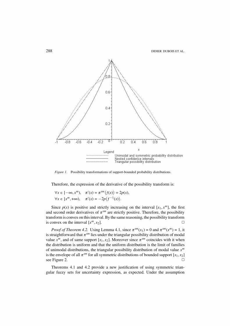
Figure 1. Possibility transformations of support-bounded probability distributions.

Therefore, the expression of the derivative of the possibility transform is:

#x % ["-, xm), "&(x) = " xm!ƒ(x)

"= 2p(x),

#x % [xm, +-), "&(x) = "2p!ƒ!1(x)

".

Since p(x) is positive and strictly increasing on the interval [x1, xm], the firstand second order derivatives of " xm are strictly positive. Therefore, the possibilitytransform is convex on this interval. By the same reasoning, the possibility transformis convex on the interval [xm, x2]. !

Proof of Theorem 4.2. Using Lemma 4.1, since " xm(x1) = 0 and " xm(xm) = 1, itis straightforward that " xm lies under the triangular possibility distribution of modalvalue xm, and of same support [x1, x2]. Moreover since " xm coincides with it whenthe distribution is uniform and that the uniform distribution is the limit of familiesof unimodal distributions, the triangular possibility distribution of modal value xm

is the envelope of all " xm for all symmetric distributions of bounded support [x1, x2]see Figure 2. !

Theorems 4.1 and 4.2 provide a new justification of using symmetric trian-gular fuzzy sets for uncertainty expression, as expected. Under the assumption


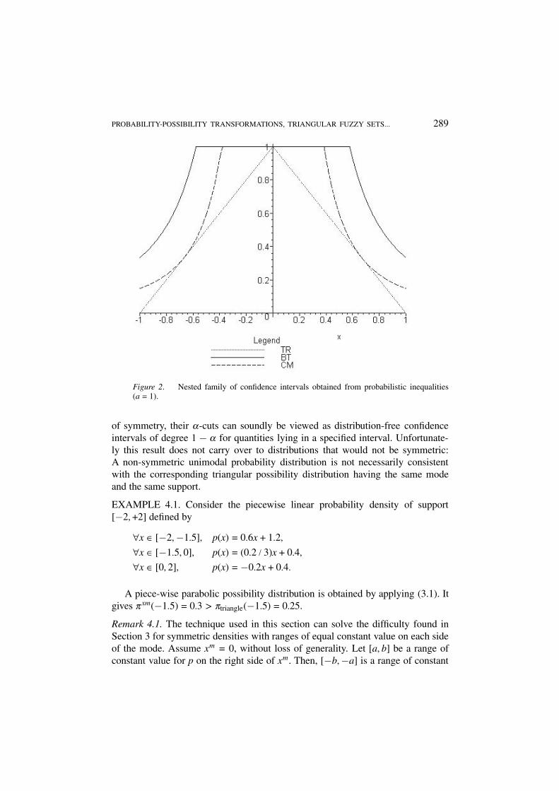
Figure 2. Nested family of confidence intervals obtained from probabilistic inequalities(a = 1).

of symmetry, their '-cuts can soundly be viewed as distribution-free confidenceintervals of degree 1 " ' for quantities lying in a specified interval. Unfortunate-ly this result does not carry over to distributions that would not be symmetric:A non-symmetric unimodal probability distribution is not necessarily consistentwith the corresponding triangular possibility distribution having the same modeand the same support.

EXAMPLE 4.1. Consider the piecewise linear probability density of support["2, +2] defined by

#x % ["2,"1.5], p(x) = 0.6x + 1.2,#x % ["1.5, 0], p(x) = (0.2 / 3)x + 0.4,#x % [0, 2], p(x) = "0.2x + 0.4.

A piece-wise parabolic possibility distribution is obtained by applying (3.1). Itgives " xm("1.5) = 0.3 > "triangle("1.5) = 0.25.

Remark 4.1. The technique used in this section can solve the difficulty found inSection 3 for symmetric densities with ranges of equal constant value on each sideof the mode. Assume xm = 0, without loss of generality. Let [a, b] be a range ofconstant value for p on the right side of xm. Then, ["b,"a] is a range of constant


(identical) value for p on the right side of xm. Then for values x and "x, wherex % [a, b], just let " xm(x) = " xm("x) = 1 " P(["x, x]). This method can be adaptedto such asymmetric densities with ranges of equal constant value on each side ofthe mode as well.

It is interesting to compare the possibility distributions obtained by the Bien-ayme-Chebychev and Camp-Meidel inequalities with the triangular fuzzy numbers.The two classical inequalities are valid for larger classes of probability distributionshence they should yield less specific bounds than the triangular fuzzy number. Con-sider a uniform probability distribution with support ["a, +a], for some positivevalue a. Its variance is * 2 = a2 / 3. Let "BT and "CM be the probability distri-butions stemming from the Bienayme-Chebychev and Camp-Meidel inequalitiesrespectively:

"BT(x) = min(1, a2 / 3x2),"CM(x) = min(1, 4a2 / 27x2),

while " xm(x) = max(0, 1" |x| /a). It is easy to verify that indeed "BT(x) % "CM(x) %" xm(x). More specifically, the differences "BT(x) " " xm(x) and "CM(x) " " xm(x) areboth minimal for x = ±2a / 3. And "CM(2a / 3) = " xm(2a / 3): The Camp-Meidel dis-tribution has a tangency point with the triangular distribution (see Figure 2). So, thetriangular fuzzy number encodes strictly better distribution-free confidence inter-vals than the Camp-Meidel inequality for support-bounded symmetric distributionswith prescribed support.

4.2. THE TRUNCATED TRIANGULAR POSSIBILITY DISTRIBUTION ANDUNBOUNDED DENSITIES

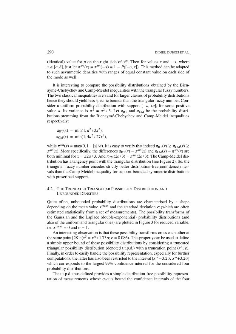
Quite often, unbounded probability distributions are characterised by a shapedepending on the mean value xmean and the standard deviation * (which are oftenestimated statistically from a set of measurements). The possibility transforms ofthe Gaussian and the Laplace (double-exponential) probability distributions (andalso of the uniform and triangular ones) are plotted in Figure 3 for reduced variable,i.e. xmean = 0 and * = 1.

An interesting observation is that these possibility transforms cross each other atthe same point [28]: (x5 = xm+1.73*; 1 = 0.086). This property can be used to definea simple upper bound of these possibility distributions by considering a truncatedtriangular possibility distribution (denoted t.t.p.d.) with a truncation point (x1 ; 1).Finally, in order to easily handle the possibility representation, especially for furthercomputations, the latter has also been restricted to the interval [xm"3.2*, xm +3.2*]which corresponds to the largest 99% confidence interval for the considered fourprobability distributions.

The t.t.p.d. thus defined provides a simple distribution-free possibility represen-tation of measurements whose '-cuts bound the confidence intervals of the four


Figure 3. Possibility distributions associated to the four considered probability laws.

probability laws. An application of this possibility expression to measurementsacquired by an ultrasonic range sensor has been presented in [27].

Note that the Bienayme-Chebychev inequality supplies a possibility distributionthat is far worse than the t.t.p.d. in terms of specificity. It is not unexpected becausethe t.t.p.d. is an approximation of the set of confidence intervals dedicated to the fourconsidered probability distributions. However, the Bienayme-Chebychev inequalitygives a set of confidence intervals valid for any probability distribution one mightchoose.

The Camp-Meidel inequality supplies a possibility distribution that it is neitherfar from what an upper bound of the four optimal possibility distributions couldbe, nor far from the t.t.p.d. Anyway, the t.t.p.d. is more interesting in terms ofspecificity. Of course, the t.t.p.d. can only be used when the probability model-ling of the measurement result can be described by one of these four probabilitydistributions.

4.3. ADDITIVE PROPAGATION OF SYMMETRIC TRIANGULAR POSSIBILITYDISTRIBUTIONS

Like in the case of random variables, possibility distributions of functions of pos-sibilistic variables can be computed by an appropriate tool called the extension


principle [39]. According to this principle, fuzzy operations are identified withinterval analysis for each cut. It thus provides a graded generalisation of intervalcalculus [4]. Moreover, the invariant forms are far more numerous for possibilitypropagation than in probability propagation, i.e. not only double exponential, andGaussian distributions [10].

A general parameterized representation of fuzzy intervals has been first proposedin [7], [10]. Let L be any u.s.c. non-increasing mapping from [0, +-) to [0, 1]satisfying the following requirements: #x > 0, L(x) < 1; #x < 1, L(x) > 0;L(0) = 1. Two cases are considered: either L(1) = 0, or L(x) > 0, #x, and then weassume that lim

x#+-L(x) = 0.

Under these requirements, L is said to be a shape function. L(x) = max(1"xn, 0),max(1 " x, 0)n, for n > 0, e!x, e!x2

, 1x + 1

are examples of shape-functions. Weconsider the class of u.s.c. fuzzy intervals whose membership function A(0) canbe described by means of two shape functions L and R and four parameters:xa

m! , xam" % R / {"-, +-}, s, t % [0, +-) having the form

A(x) = L!(xa

m! " x) / s"

#x < xam! ,

A(x) = 1 if x % [xam! , xa

m"],

A(x) = R!(x " xa

m") / t

"#x > xa

m".

For s = 0 (resp. t = 0), A(x) = 0 when x < xam! (resp. x > xa

m"), by convention. A

fuzzy interval A described as above is called an LR-fuzzy interval and the notationA = (xa

m! , xam", s, t)LR is adopted. L and R are called the left shape and the right shape

functions, respectively. The parameters s and t are called the left spread and theright spread, respectively.

The addition of fuzzy numbers is a possibilistic counterpart to the convolutionof random variables. The sum A 2 B of A and B is defined by the sup-min extensionprinciple:

A 2 B(z) = supx

min!A(x), B(z " x)

".

The following result was pointed out in [7], [10] for the addition of L-R fuzzynumbers of the form A = (xa

m! , xam", s, t)LR and B = (xb

m! , xbm", u, v)LR:

A 2 B = (xam! + xb

m! , xam" + xb

m", s + u, t + v)LR.

The cuts (A 2 B)' can be obtained by applying interval arithmetic to the '-cutsA' and B' . So, the addition of two triangular symmetric possibility distributionsof support [xa

1 , xa2] (respectively [xb

1 , xb2]) and of mode xa

m (respectively xbm) is the

triangular possibility distribution of support [xa1 +xb

1 , xa2 +xb

2] and of mode xam+xb

m.

THEOREM 4.3. Let A and B be two symmetric triangular fuzzy numbers. Themembership function of A 2 B is a possibility distribution consistent with the sum(by regular convolution) of any two symmetric probability distributions having thesame supports as A and B respectively.


Proof. The addition of A and B by the sup-min extension principle yields asymmetric triangular fuzzy number. Due to Theorem 4.2, the symmetric triangularfuzzy number is the maximally specific possibility distribution consistent with allthe bounded symmetric probability distributions with the same support. Obviously,the probability density of the random addition of any two symmetric probabilitydistributions pa and pb having supports [xa

1 , xa2] and [xb

1 , xb2] is symmetric, has

support [xa1 + xb

1 , xa2 + xb

2], and therefore is consistent with the triangular distributionobtained by the addition of the two triangular possibility distributions. Hence A 2 Bis less specific than the possibilistic transforms of the result of the convolution ofpa and pb. !

Remark 4.2. The same theorem holds for the subtraction. However it generally willnot hold for other type of operations, nor for any shape-function, nor for asymmetricfuzzy numbers.

5. Application to the Representation of Uncertainty in Measurement

Generally, the acquisition of information by measurement systems is not perfect, i.e.not totally corresponding to the observed phenomena. The reasons for imperfectionare various: approximate definition of the measurand, limited knowledge of theenvironment context, variability of influence quantities, and so on. These effects leadto shifts and/or to fluctuations of the values, i.e. uncertainties. Representing theseuncertainties is an old issue in science, but the norm to deal with these uncertainties isquite recent. Indeed, the ISO Guide for the expression of uncertainty in measurement[20] prepared under the aegis of the main international organisations in metrology:!

BIPM, IEC, ISO, OIML, has been published in 1993.According to this ISO Guide, the expression of measurement uncertainty must

satisfy some requirements in order to be widely used at the practical level. TheGuide recommends a parametric representation of the measurement uncertaintywhich:

a) characterises the dispersion of the observed values; for example the standarddeviation or half the width of an interval at a given level of confidence,

b) can provide a confidence interval which contains an important proportion ofthe observed values,

c) can be easily propagated in further processing.

Thus, the ISO Guide proposed to characterise the measurement result by thebest estimation of the measurand (i.e. in general the mean value) and the standarddeviation. In fact, it simplifies the probability approach by considering only thefirst two moments (mean value, variance) of the probability distribution. In the

! BIPM: Bureau International des Poids et Mesures; IEC: International Electro-technical Commit-tee; ISO: International Organization for standardization; OIML: International Organization of LegalMetrology.


fuzzy/possibility representation proposed before, the best estimation is simply thevalue which has membership degree 1, i.e. the modal value. Using the horizontalview of a fuzzy subset, each cut defines an interval of confidence 1" '. Therefore,the fuzzy/possibility representation is compatible with the Guide, especially withthe second aspect of point (a), and moreover provides the intervals for the wholeset of levels of confidence, and not only for an arbitrary one, e.g. 99%. Note thatthere are many probability distributions corresponding to the prescribed mode andgiven confidence intervals, e.g. for 0.5 and 0.95. One practical difficulty with thechoice of the mode for a representative value is that it is less easy to estimate thanfor instance the mean value. Recent proposals such as so called rough histograms(Strauss et al. [37]), where the partition underlying histograms is changed into afuzzy partition, may provide robust estimators of the mode.

This is coherent with the fact that a possibility distribution is an upper bound ofa family of probability distributions. The level of confidence 1"' is a lower boundof the probability that the value belongs to the interval I' . This representation isthus not equivalent to the definition of one single probability distribution, and isparticularly interesting for the expression of the so-called uncertainty of type B(i.e. those are evaluated by other means than statistical methods). As illustratedby many examples in the ISO Guide, an uncertainty of type B is often given byexperts under the form of a few intervals (but not all of them) correspondingto particular levels of confidence, generally 0 and 1 [27]. Therefore, building apossibility distribution from these intervals sounds a more natural method thanderiving the standard deviation since the latter requires assumptions on the shapeof the probability law which is often a priori unknown in theses cases. Moreover,defining a possibility distribution by linear interpolation between the consideredinterval bounds is well-founded as demonstrated in Section 3.

6. Conclusion

This paper has proposed a systematic approach for the transformation of a con-tinuous probability distribution into a maximally specific possibility distributionthat enables upper bounds of probabilities of events to be computed. The obtainedpossibility distribution encodes a nested family of tightest confidence intervalsaround the mode of the statistical distribution considered. There are of course oth-er transformations from probability to possibility [6], [15], [16], [31], [32]. Theone proposed here aims at preserving as much of the information contained inthe probability distribution one starts with. Each '-cut of the obtained possibilitydistribution is the smallest (hence the most informative) interval one may use inplace of the probability distribution, with a guarantee that the probability that theunknown parameter of interest lies in this interval is at least 1 " '.

Moreover, a possibility-theoretic interpretation of probabilistic inequalities suchas Bienayme-Chebychev and Camp-Meidel inequalities has been suggested.Applied to support-bounded densities, this result provides a new justification of


triangular fuzzy numbers for representing uncertainty within an interval. Indeed,the triangular possibility distribution is an optimal transform of the uniform prob-ability distribution and it is the upper envelope of all the possibility distributionstransformed from symmetric probability densities with the same support. It yieldsbetter confidence intervals for this class of distributions than the Camp-Meidelinequalities.

As an application, a new procedure for a fuzzy/possibility expression of mea-surement uncertainty has been outlined, based on these results. It uses the truncatedtriangular possibility distribution obtained as an approximation of four standarddensities. At the operational level, the proposed expression is compatible with theISO Guide of expression of uncertainty in measurement. When the uncertaintyis expressed by a standard deviation only, then a better specificity is obtained byusing the triangular possibility distribution than the ttpd. But, when the uncertaintyis only expressed by the range of the set of measures, then a better specificity isobtained by using the truncated triangular possibility distribution. It is then uselessto compute a standard deviation from the supplied range of measures in the lattercase. And finally, when the range and the standard deviation are both supplied, thenthe greater the standard-deviation/range ratio will be, the more useful the triangularpossibility distribution will be.

Further research should consider the propagation of the proposed fuzzy/possibility expression of measurement uncertainty, and the extent to which it canbe used as a substitute to a plain random variable propagation. If this question issimple (as shown above) for operations like the addition or the subtraction whichpreserve the symmetry of probability distribution, it is more difficult for operationslike division which do not preserve symmetry. It presupposes a deeper study of thepossibility transforms of unimodal but asymmetric probability distributions. Canasymmetric triangular fuzzy numbers be used? As mentioned before, an importantpoint is then to choose the nominal value, i.e. the value x" used in definition 1.Must it be the modal, the mean or the median value ? It seems that this choice mustbe made before building a distribution-free possibility representation in order tobe able to find an adequate family of nested intervals to be used in an operationaldefinition of a consistent possibility distribution.

Acknowledgement

Authors are indebted to V. Lasserre for her early contribution to some parts of thiswork.

References

1. De Cooman, G. and Aeyels, D.: A Random Set Description of a Possibility Measure and ItsNatural Extension, IEEE Trans on Systems, Man and Cybernetics 30 (2000), pp. 124–131.

2. De Cooman, G. and Aeyels, D.: Supremum-Preserving Upper Probabilities, Information Sciences118 (1999), pp. 173–212.


3. Delgado, M. and Moral, S.: On the Concept of Possibility-Probability Consistency, Fuzzy Setsand Systems 21 (1987), pp. 311–318.

4. Dubois, D., Kerre, E., Mesiar, R., and Prade, H.: Fuzzy Interval Analysis, in: Dubois, D. andPrade, H. (eds), Fundamentals of Fuzzy Sets, The Handbooks of Fuzzy Sets Series, KluwerAcademic Publishers, Boston, USA, 2000, pp. 483–581.

5. Dubois, D., Nguyen, H. T., and Prade, H.: Possibility Theory, Probability and Fuzzy Sets:Misunderstandings, Bridges and Gaps, in: Dubois, D. and Prade, H. (eds), Fundamentals ofFuzzy Sets, The Handbooks of Fuzzy Sets Series, Kluwer Academic Publishers, Boston, USA,2000, pp. 343–438.

6. Dubois, D. and Prade, H.: Consonant Approximations of Belief Functions, Int. J. ApproximateReasoning 4 (1990), pp. 419–449.

7. Dubois, D. and Prade, H.: Fuzzy Sets and Systems: Theory and Applications, Academic Press,New York, 1980.

8. Dubois, D. and Prade, H.: Fuzzy Sets, Probability and Measurement, European Journal ofOperational Research 40 (1989) pp. 135–154.

9. Dubois, D. and Prade, H.: On Several Representations of an Uncertain Body of Evidence, in:Gupta, M. M. and Sanchez, E. (eds), Fuzzy Information and Decision Processes, North-Holland,1982, pp. 167–181.

10. Dubois, D. and Prade, H.: Operations on Fuzzy Numbers, Int. J. Systems Science 9 (1978)pp. 613–626.

11. Dubois, D. and Prade, H.: Possibility Theory: An Approach to Computerized Processing ofUncertainty, Plenum Press, New York, 1988.

12. Dubois, D. and Prade, H.: Qualitative Possibility Theory and Its Applications to ConstraintSatisfaction and Decision under Uncertainty, Int. Journal of Intelligent Systems 14 (1999),pp. 45–61.

13. Dubois, D. and Prade, H.: The Three Semantics of Fuzzy Sets, Fuzzy Sets and Systems 90 (1997),pp. 141–150.

14. Dubois, D. and Prade, H.: When Upper Probabilities Are Possibility Measures, Fuzzy Sets andSystems 49 (1992), pp. 65–74.

15. Dubois, D., Prade, H., and Sandri, S.: On Possibility/Probability Transformations, in:Lowen, R. and Roubens, M. (eds), Fuzzy Logic, Kluwer Academic Publishers, Dordrecht, 1993,pp. 103–112.

16. Dubois, D., Prade, H., and Smets, P.: New Semantics for Quantitative Possibility Theory, in:Proc.of the 6th European Conference on Symbolic and Quantitative Approaches to Reasoningand Uncertainty (ESQARU 2001), Toulouse, France, LNAI 2143, Springer-Verlag, Berlin, 2001,pp. 410–421.

17. Dubois, D., Prade, H., and Smets, P.: Representing Partial Ignorance, IEEE Trans. on Systems,Man and Cybernetics 26 (1996), pp. 361–377.

18. Geer, J. F. and Klir, G.: A Mathematical Analysis of Information-Preserving Transformationsbetween Probabilistic and Possibilistic Formulations of Uncertainty, Int. J. of General Systems20 (1992), pp. 143–176.

19. Goodman, I. R. and Nguyen, H. T.: Uncertainty Models for Knowledge-Based Systems, North-Holland, Amsterdam, 1985.

20. Guide for the Expression of Uncertainty in Measurement, ISO 1993, 1993.21. Kendall, M. and Stuart, A.: The Advanced Theory of Statistics, Ed. Griffin and Co., 1977.22. Jamison, K. D. and Lodwick, W. A.: The Construction of Consistent Possibility and Necessity

Measures, Fuzzy Sets and Systems 132 (2002), pp. 65–74.23. Higashi, M. and Klir, G.: Measures of Uncertainty and Information Based on Possibility Distri-

butions, Int. J. General Systems 8 (1982), pp. 43–58.24. Klir, G. J.: A Principle of Uncertainty and Information Invariance, Int. Journal of General Systems

17 (1990), pp. 249–275.25. Klir, G. J. and Parviz, B.: Probability-Possibility Transformations: A Comparison, Int. J. of

General Systems 21 (1992), pp. 291–310.26. Lasserre, V.: Modelisation floue des incertitudes de mesures de capteurs, Ph. D. Thesis, University

of Savoie, Annecy, France, 1999.


27. Mauris, G., Berrah, L., Foulloy, L., and Haurat, A.: Fuzzy Handling of Measurement Errors inInstrumentation, IEEE Trans. on Measurement and Instrumentation 49 (2000), pp. 89–93.

28. Mauris, G., Lasserre, V., and Foulloy, L.: A Fuzzy Approach for the Expression of Uncertaintyin Measurement, Int. Journal of Measurement 29 (2001), pp. 165–177.

29. Mauris, G., Lasserre, V., and Foulloy, L.: Fuzzy Modeling of Measurement Data Acquired fromPhysical Sensors, IEEE Trans. on Measurement and Instrumentation 49 (2000), pp. 1201–1205.

30. McCain, R. A.: Fuzzy Confidence Intervals, Fuzzy Sets and Systems 10 (1983), pp. 281–290.31. Moral, S.: Constructing a Possibility Distribution from a Probability Distribution, in: Jones, A.,

Kauffmann, A., and Zimmermann, H. J. (eds), Fuzzy Sets Theory and Applications, D. Reidel,Dordrecht, 1986, pp. 51–60.

32. Oussalah, M.: On the Probability/Possibility Transformations: A Comparative Analysis, Int.Journal of General Systems 29 (2000), pp. 671–718.

33. Pedrycz, W.: Why Triangular Membership Functions?, Fuzzy Sets and Systems 64 (1994),pp. 21–30.

34. Shackle, G. L. S.: Decision Order and Time in Human Affairs, Cambridge University Press,1961.

35. Smets, P.: Constructing the Pignistic Probability Function in a Context of Uncertainty, in: Hen-rion, M., Schachter, R. D., Kanal, L. N., and Lemmer, J. F. (eds), Uncertainty in ArtificialIntelligence, North-Holland, Amsterdam, 1990, pp. 29–40.

36. Smets, P.: Decision Making in a Context Where Uncertainty Is Represented by Belief Functions,in: Srivastava, R. P. (ed.), Belief Functions in Business Decisions, Physica-Verlag, Heidelberg,2001.

37. Strauss, O., Comby, F., and Aldon, M.-J.: Rough Histograms for Robust Statistics, in: IEEE Int.Conf. On Pattern Recognition (ICPR’00), Barcelona, 2000, pp. 2684–2687.

38. Wang, P. Z.: From the Fuzzy Statistics to the Falling Random Subsets, in: Wang, P. P. (ed.),Advances in Fuzzy Sets, Possibility Theory and Applications, Plenum Press, New York, 1983,pp. 81–96.

39. Zadeh, L. A.: Fuzzy Sets, Information and Control 8 (1965), pp. 338–353.40. Zadeh, L. A.: Fuzzy Sets as a Basis for a Theory of Possibility, Fuzzy Sets and Systems 1 (1978),

pp. 3–28.

Documents

P robability-P ossibility T ransform ations, T riangular F ...Henri.Prade/Papers/DFoulMauP.pdf · P robability-P ossibility T ransform ations, T riangular F uzzy S ets, and P robabilistic