P) Ehrenberg-Oaxaca_1976_Unemployment insurance duration of unemployment.pdf

American Economic Association

Unemployment Insurance, Duration of Unemployment, and Subsequent Wage GainAuthor(s): Ronald G. Ehrenberg and Ronald L. OaxacaSource: The American Economic Review, Vol. 66, No. 5 (Dec., 1976), pp. 754-766Published by: American Economic AssociationStable URL: http://www.jstor.org/stable/1827489 .

Accessed: 27/06/2013 17:16

Your use of the JSTOR archive indicates your acceptance of the Terms & Conditions of Use, available at .http://www.jstor.org/page/info/about/policies/terms.jsp

.JSTOR is a not-for-profit service that helps scholars, researchers, and students discover, use, and build upon a wide range ofcontent in a trusted digital archive. We use information technology and tools to increase productivity and facilitate new formsof scholarship. For more information about JSTOR, please contact [email protected].

.

American Economic Association is collaborating with JSTOR to digitize, preserve and extend access to TheAmerican Economic Review.

http://www.jstor.org

This content downloaded from 200.24.23.76 on Thu, 27 Jun 2013 17:16:25 PMAll use subject to JSTOR Terms and Conditions

http://www.jstor.org/action/showPublisher?publisherCode=aea

http://www.jstor.org/stable/1827489?origin=JSTOR-pdf

http://www.jstor.org/page/info/about/policies/terms.jsp


Unemployment Insurance, Duration of

Unemployment, and Subsequent

Wage Gain

By RONALD G. EHRENBERG AND RONALD L. OAXACA*

Recent debate over potential methods to reduce the unemployment rate has

.stressed the impact of the unemployment insurance (UI) system, arguing that liberal benefit levels tend to increase the level of unemployment.' That the system may have this effect in the short run should not be surprising in that an explicit objective of the UI system is to provide temporary income maintenance for unemployed workers, so as to allow them to reject job offers substantially below their skill levels and to engage in productive job search.2 Indeed all formal analytic models of job search imply that increases in UI benefit levels will both increase unemployed workers' expected durations of unemployment and their expected postunemployment wages.3 Consequently, any discussion of' the appropriate level of UI benefits must con- sider this intertemporal tradeoff and evaluate whether the cost to society of increased durations of spells of unemployment when UI benefits are raised is more than off-

set by the increases in expected postunemployment wages.

In order to evaluate what the "optimal" level of UI benefits is, one must therefore first estimate the magnitude of the rela-' tionships between UI benefits' levels and unemployed workers' durations of unemployment and postunemployment -wages. There have been several previous studies of the impact of UI benefits on duration of spells of unemployment, however none have been completely satisfactory meth- odologically.4 To our knowledge, there have been no previous studies of the system's impact on subsequent wage rates.5 We attempt to fill these gaps, utilizing data from the National Longitudinal Sur- vey (NLS) to estimate both relationships.

The plan of our paper is as follows. First, we sketch the implications of theories of job search for our estimating equations. Next, we briefly discuss the NLS data. The following four sections summarize the empirical results we have obtained for four cohorts of data: older males, ages 45-59; Women, ages 30-44; and younger males

* Associate professor of economics and labor economics, Cornell University, and associate professor of economics, University of Arizona. This paper sum- marizes the results of research supported under U.S. Department of Labor Contract L74-49, however the views expressed here are solely the responsibility of the authors. We are deeply indebted to Edward Karl for his research assistance during the course of the study. An earlier version of this paper was delivered at the Third World Congress of the Econometric Society.

'See for example, Martin Feldstein (1973). ' See William Haber and Merrill Murray, pp. 26-35. 'See for example, Dale Mortensen. Kenneth Bur-

dett surveys these theories and emphasizes the importance of each of the various assumptions cus- tomarily made in models of this type.

' Many of these studies are enumerated in Ehren- berg (1974). By far the best appears to be by Ronald Schmidt, who is concerned primarily with testing the implications of search theory rather than with estimating the impact of UI benefits. Stephen Marston presents an approach which is quite different from that found in most of the studies, including our own.

Kathleen Classen has attempted to estimate the system's impact on workers' annual and high quarter earnings, using data from the Continuous Wage and Benefit History File for Pennsylvania. Unfortunately, this data base has numerous weaknesses as compared to the NLS data used in this study (see Ehrenberg, 1975).

754



VOL. 66 NO. 5 EHRENBERG AND OAXACA: UNEMPLOYMENT INSURANCE 755

and females, ages 14-24. Finally, we con- sider the implications of our results for public policy. Due to space limitations our discussion here is necessarily brief and details of our research are found elsewhere.6

I. Implications of Theories of Job Search

Numerous models of unemployed workers' job search under imperfect information have been developed during the past few years. While the specific form of the solution to the individual's decision problem depends on the specific assumptions made, the implications of these models for unemployed workers' expected durations of spells of unemployment (E(D)) and expected postunemployment wages (E(W)) are fairly robust and appear to be invari- ant to many of the assumptions. These implications include:

(i) Anything that reduces the cost of being unemployed (c) will increase an individual's expected duration of unemployment and expected postunemployment wage.

(ii) Anything that decreases an individual's horizon (n) will decrease his expected duration of spell and postunemployment wage.

(iii) Anything that influences an individual's skill level (s) will increase his expected postunemployment wage but may have an ambiguous effect on expected duration.7

(iv) Anything that increases the individual's discount rate (r) will reduce his search and lead to a decrease in both his expected duration of spell and postunemployment wage.

(v) Anything that influences the distribution of potential wage offers (d) that an unemployed individual faces will in-

fluence his expected postunemployment wage and duration of spell.

Thus, models of job search under imperfect information suggest a two-equation .model of the determinants of an individual's expected duration of unemployment and postunemployment wage of the form

(1) E(D) = f(c,n,s,r,d).

(2) E(W) = g(c,n,s,r,d)

Two comments should be made about this system of equations. First, as indicated in an appendix which is available from us on request, if rigorously applied, the theory implies not only qualitative implications about the partial derivatives in (1) and (2) but also cross-equation restric- tions on both their functional forms and the magnitudes of corresponding coefficients in the two equations. Second, as Feldstein has emphasized,' in estimating the cost of remaining unemployed, the individual should rationally compare UI benefit payments to net after-tax potential earnings.8 This occurs because UI benefits are not taxable, while federal and state income taxes and social security taxes must be paid on labor earnings. Conse- quently,. the cost of remaining unemployed is given by

(3) C= Wp(l-t)Bk

where W, is the individual's potential weekly earnings, t is his marginal tax rate, B is his weekly UI benefit level, and k is a parameter that varies across individuals which, if greater than one, indicates that the individual is receiving supplementary unemployment benefits from private sources.

Empirically, due to data limitations, we are forced to assume that W, equals the preunemployment weekly wage and that

6 See Ehrenberg (1974) and the authors. 7 Heuristically, this ambiguity occurs because in-

creasing an individual's skill level increases the proportion of jobs for which he is eligible and also induces him to reject a greater proportion of low wage offers.

'See Feldstein (1973). Presumably all work-related expenses should also be subtracted from potential earnings in this calculation.



756 THE AMERICAN ECONOMIC REVIEW DECEMBER 1976

k equals unity for all individuals.9 Then (3) can be written

(3') C = W (1-t)[ -'F/(1 - ))]

where F is the replacement fraction, the ratio of an individual's weekly UI benefits to his' preunemployment weekly wage. This variable.is a policy instrument and varies across individuals due to the liberal- ity of various state plans, the level of the individuals' -previous earnings, and their number of dependents. Our empirical work focuses on estimating the impact of this variable on unemployed workers' expected. durations of unemployment and postunemployment wages.

II. The National Longitudinal Survey (NLS) Data

Our empirical analysis utilizes data con- tained in the NLS sample..The survey was conducted by the U.S. Bureau'of the Census for the Manpower Administration, and the data files are currently distributed by the Center for Human Resource Re- search at Ohio State University. This longitudinal survey contains a' wealth of information relating to the labor force behavior of four cohorts of 5000 individuals each: older males, ages 45-59; women, ages 30-44; and young males and females, ages 14-24 at their initial survey 'dates.'0

Although the state that' each individual is located in is not explicitly reported in the public use version of the NLS tapes, .it proved possible for us to infer each individual's state of residence from other information which was provided. This allowed us to estimate each unemployed individual's state and federal marginal income tax rate, and his marginal social

security tax rate.'1 In addition, it allowed us to merge additional. data relating to specific' state unemployment insurance systems with each individual's record. At points in our empirical work, we: were thus able to estimate the impact of such state UI system parameters as the maximum duration of weeks of benefit payments, the length of the' waiting period before benefits start, the denial rate and the coverage rate on unemployed individuals' job search behavior.

lII. Empirical Results-Older Males Our initial analysis was conducted using

the older male data. At the time our study was started, annual surveys for this cohort had been conducted and were available for the 1966-69 period. However, the .1968 survey was an abbreviated mail one which did not contain information on wage rates or numbers of spells of unemployment. In order to estimate both the postunemployment. wage and 'average duration of unemployment equations with as little measurement error as possible in the explanatory variables, we confined our analysis to data from the 1966.and 1967 surveys. We utilized a sample of 274 men who a) were employed wage and salary workers and reported their wage rates at both dates, b) were unemployed. sometime during the interim, and c) reported their number of spells and whether they received- un- employment insurance benefits during the period.'2 This sample. was further strati- fied, and separate equations estimated for individuals who were voluntarily un-

9A discussion of how these assumptions bias our coefficient estimates is found in Ehrenberg (1974).

1" See the Center for Human Resource Research and Herbert Parnes for a description of the survey. The strengths and weaknesses of this data set for UI research are described.in detail in Ehrenberg (1975).

"See Ehrenberg (1974) for a description of our methodology.

"Data from the 1968 and 1969 surveys could have been used in an analogous manner if we were willing to use the 1967 wage as a proxy for the 1968 wage in the duration and wage gain equations. Although we have subsequently made similar imputations (see below) for the female cohort to increase the sample size, we attempted in our initial analysis to keep the data as *free of measurement error as possible.




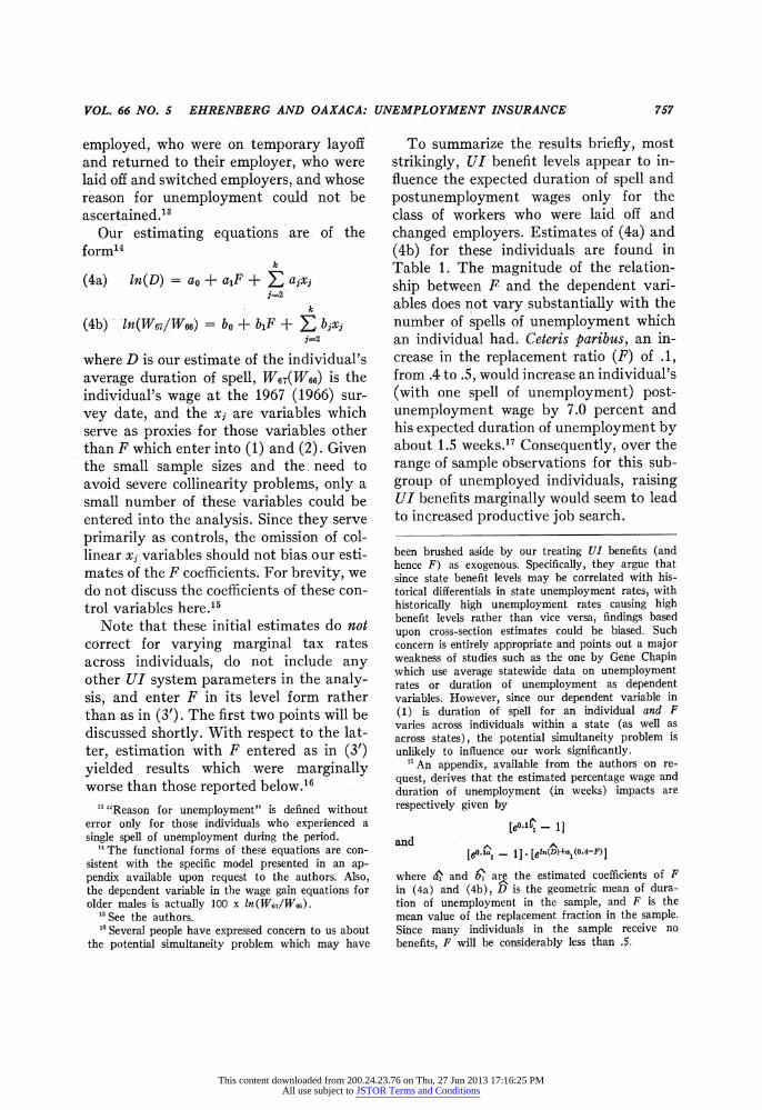
employed, who were on temporary layoff and returned to their employer, who were laid off and switched employers, and whose reason for unemployment could not be ascertained.13

Our estimating equations are of the form'4

k

(4a) ln(D) = ao + ajF + Z a1x1 j=2

k

(4b) In(W67/W66) = bo + bjF + , bjxj j=2

where D is our estimate of the individual's average duration of spell, W67(W66) is the individual's wage at the 1967 (1966) survey date, and the xj are variables which serve as proxies for those variables other than F which enter into.(1) and (2). Given the small sample sizes and the. need to avoid severe collinearity problems, only a small number of these variables could be entered into the analysis. Since they serve primarily as controls, the omission of col- linear xj variables should not bias.our estimates of the F coefficients. For brevity, we do not discuss the coefficients of these control variables here."5

Note that these initial estimates do not correct for varying marginal tax rates across individuals, do not include any other UI system parameters in the analysis, and enter F in its level form rather than as in (3'). The first two points will be discussed shortly. With respect to the latter, estimation with F entered as in (3') yielded results which were marginally worse than those reported below.16

To summarize the results briefly, most strikingly, UI benefit levels appear to influence the expected duration of spell and postunemployment wages only for the class of workers who were laid off and changed employers. Estimates of (4a) and (4b) for these individuals are found in Table 1. The magnitude of the relation- ship between F and the dependent variables does not vary substantially with the number of spells of unemployment which an individual had. Ceteris paribus, an increase in the replacement ratio (F) of .1, from .4 to .5, would increase an individual's (with one spell of unemployment) postunemployment wage by 7.0 percent and his expected duration of unemployment by about 1.5 weeks.17 Consequently, over the range of sample observations for this sub- group of unemployed individuals, raising UI benefits marginally would seem to lead to increased productive job search.

i3 "Reason for unemployment" is defined without error only for those individuals who experienced a single spell of unemployment during the period.

14The functional forms of these. equations are con- sistent with the specific model presented in an appendix available upon request to the authors. Also, the dependent variable in the, wage gain equations for older males is actually 100 x In(W67/W66).

15 See the authors. 1G Several people have expressed concern to us about

the potential simultaneity problem which may have

been brushed aside by our treating UI benefits (and hence F) as exogenous. Specifically, they argue that since state benefit levels may be correlated with his- torical differentials in state unemployment rates, with historically high unemployment rates causing high benefit levels rather than vice versa, findings based upon cross-section estimates could be biased. Such concern is entirely appropriate and points out a major weakness of studies such as the one by Gene Chapin which use average statewide data on unemployment rates or duration of unemployment as dependent variables. However, since our dependent variable in (1) is duration of spell for an individual and F varies across individuals within a state (as well as across states), the potential simultaneity problem is unlikely to influence our work significantly.

17 An appendix, available from the authors on request, derives that the estimated percentage wage and duration of unemployment (in weeks) impacts are respectively given by

Ieo1 - 1] and

le?.lal - 1]. [en(D)+aI(0.4-F)I

where 6i and 6\ are the estimated coefficients of F in (4a) and (4b), D is the geometric mean of duration of unemployment in the sample, and F is the mean value of the replacement fraction in the sample. Since many individuals in the sample receive no benefits, F will be considerably less than .5.




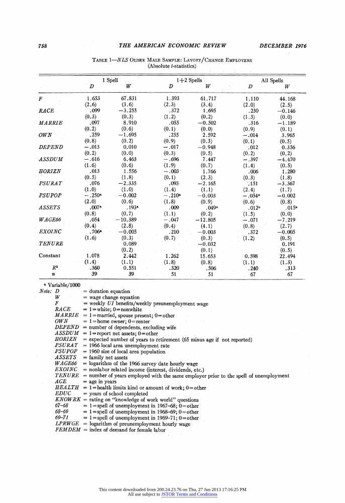
TABLE 1-NLS OLDER MALE SAMPLE: LAYOFF/CHANGE EMPLOYERS (Absolute t-statistics)

1 Spell 1+2 Spells: All Spells D W D W D W

F 1.653 67.831 1.393 61.717 1.110 44.168 (2.6) (3.6) (2.3) (3.4) (2.0) (2.5)

RACE .099 -3.255 .372 1.695 .230 -0.146 (0.3) (0.3) (1.2) (0.2) (1.3) (0.0)

MARRIE .097 8.910 .055 -0.502 .316 -1.189 (0.2) (0.6) (0.1) (0.0) (0.9) (0.1)

OWN .259 -1.695 .255 2.592 --.014 3.965 (0.8) ~ (0.2) (0.9) (0.3) (0.1) (0.5)

DEPEND - .013 0.010 - .017 -0.948 .012 0.356 (0.2) (0.0) (0.3) (0.5) (0.2) (0.2)

ASSDUM - .616 6.463 - .696 7.447 - .397 -4.470 (1.6) (0.6) (1.9) (0.7)- (1.4) (0.5)

HORIZN .013 1.556 - .003 1.766 .006 1.280 (0.5) (1-.8) (0.1) (2.3) (0.3) (1.8)

PSURAT .076 -2.335 .093 -2.165 .151 -3.367 (1.0) (1.0) (1.4) (1.1) (2.4) (1.7)

PSUPOP -.250a -0.002 -.2108 -0.003 - .054a -0.002 (2.0) (0.6) (1.8) (0.9) (0.6) (0.8)

ASSETS .007a .193a .009 .049a .012a .015a (0.8) (0.7) (1.1) (0.2) (1.5) (0. 0)

WAGE66 .054 10.389 - .047 -12.805 - .071 -7.219 (0.4) (2.8) (0.4) (4.1) (0.8) (2.7)

EXOINC .7068 -0.005 .210 -0.003 .372 -0.005 (1.6) (0.3) (0.7) (0.3) (1.2) (0.5)

TENURE 0.089 -0.032 0.191 (0.2) (0.1) - (0.5)

Constant - 1 . 078 2.442 1.262 15.653 0.598 22.494 (1.4) (1.1) (1.8) (0.8) (1.1) (1.3)

R2 .360 0.551 .320 .506 .240 .313 n 39 39 51 51 67 67

Variable/1000 Note: D = duration equation

W - = wage change equation F = weekly Ul benefits/weekly preunemployment wage RACE = 1 =white; 0=nonwhite MARRIE = 1 = married, spouse present; 0= other OWN = 1 =home owner; 0= renter DEPEND = number of dependents, excluding wife ASSDUM = 1= report net assets; 0 = other HORIZN = expected number of years to retirement- (65 minus age if not reported) PSURAT = 1966'local area unemployment rate PSUPOP = 1960 size of local area population ASSETS = family net assets WAGE66 = logarithm of the 1966 survey date hourly wage EXOINC = nonlabor related income (interest, dividends, etc.) TENURE = number of years employed with the same employer prior to the spell of unemployment AGE = age in years HEALTH = 1 =health limits kind or amount of work; 0= other EDUC -years of school completed KNOWRK = rating on "knowledge of work world" questions 67-68 -1 = spell of unemployment in 1967-68; 0'= other 68-69 = 1=spell of unemployment in 1968-69; 0= other 69-71 = 1=spell of unemployment in 1969-71; 0=other LPRWGE = logarithm of preunemployment hourly wage FEMDEM = index of demand for female labor




RELLFP = fraction of years since high school in the labor force RELDUM = 1 = not report RELLFP; 0 = other PERCPY = per capita family income, excluding the respondent's income NREPY = 1 =not report PERCPY; 0 = other HUSBY = husband's income NASSDM = 1 = not report net assets; 0= other

Several extensions of this analysis war- rant being reported here."8 First, the magnitudes of the replacement ratio coefficients are fairly insensitive to the specific (if any) control variables included and the exclusion of individuals with zero UI benefits from the sample. Second, adjusting the data for marginal tax rates, which varied across individuals, altered the results only slightly and. did not significantly change the quantitative impacts of UI benefits on job search. Finally, including the other UI system parameters in the model did not significantly improve the explanatory power.. of the model nor did any of these coefficients prove to be statistically significant. We caution, however, that the fact that the coefficient of the maximum number of weeks of potential duration of benefits is insignificant. sheds no light on the effect on expected duration of unemployment of the Federal Extended Benefit and Supplementary Benefit Programs which raised the potential duration. (in early 1976) to 65 weeks. The individuals in our sample of older men all tended to have extremely short spells. of unemployment and the proportion of individuals exhausting benefits is much higher today.

IV. Empirical Results-Women

Annual surveys for the cohort of women ages 30-44 in 1967 were available to us for 1967 .(with retrospective. information for 1966), 1968 (mail survey), 1969, and 1971. We divided these data into three periods: 1966-67, .1968-69, and .1969-71. An individual was included in our sample for a period if she a) was an employed wage and

salary worker and reported her wage at both survey dates, b) was unemployed some time during the interim, and c) reported her number of spells of unemployment. The three samples were then pooled together to create one overall sample of 441 individuals. Due to errors in our measurement of the 1966 wage, it was impossible for us to estimate a wage gain equation for the 1966-67 sample and that period's data also did not permit us to identify whether or not the individual had changed employers. Consequently, we created two other samples of individuals: all who fell in the 1968-69 and 1969-71 samples (253) and those who changed employers and fell in these samples (156).19

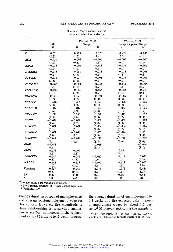
Equations similar to (4a) and (4b) were estimated for:these three samples, with the dependent variable in (4b) being the logarithm of the ratio of the wage rates at the, two survey dates. The results are presented in Table 2.20 The control variables included in the analysis are different from those in the previous section because of the different nature of the two samples and the larger number of observations available here.

Similar to the older male results, UI benefits are seen to influence both the

18See Ehrenberg (1974).

19 In this sample, and those of the following sections, a few individuals were unemployed in more than one year. The inclusion of these repeaters introduces some correlation of residuals across equations. However, experiments indicated* that excluding these repeaters yielded virtually identical results. These data also did not permit us to identify voluntary and involuntary separations.

20Actually the dependent variables were '2 log (W69/W67) and Y2 log (W71/W69), respectively, so as to capture annual growth rates. W67 was used as a proxy for Ws8, which was not reported in the mail survey of 1968.




TABLE 2-NLS FEMALE SAMPLEa

(absolute value t statistics)

1968-69; 69-71 1968-69; 70-71 All Sample Change Employer Sample D - D W D W

F 0.371 0.295 0.120 0.428 0.145 (2.5) (1.7) (4.4) (2.0) (4.2)

AGE 0.021 0.006 -0.006 -0.009 -0.009 (1.7) (0.3) -(2.3) (0.4) (2.6)

RACE -0.235 -0.003 -0.013 -0.036 -0.006 (2.0) (1.7) (0.5) (0.2) (0.2)

MARRIE -0.075 -0.288 0.015 -0.412 0.031 (0.6) (1.7) (0.6) (1.8) (0.8)

PSURAT 0.036 0.037 0.004 0.036 0.004 (1.3) (1.1) (0.7) (0.7) (0.4)

PSUPOPb 0.087 0.082 0.025 0.113 0.038 (1.8) (1.2) (2.2) (1. 1) (2.2)

FEMDEM 0.020 0.021 -0.567 0.028 -0.240 (1.8) -(1.4) (0.2) (1.3) (0. 1)

DEPEND 0.021 0.074 -0.010 0.066 -0.011 (0'.7) (1.7) (1.4) (1.-0) (1. 1)

RELLFP -0.516 -0.301 0.021 -0.398 0.025 (2.8) (1.2) (0.6) (1.2) (0.5)

RELDUM 0.012 -0.042 0.094 -0.037 0.055 (0.6) (0.2) (2.3) (0.1) (0.9)

HEALTH 0.236 0.383 0.098 0.072 0.072 (1.5) (1.8) (2.9) (0.2) (1.4)

EDUC -0.029 -0.052 0.009 -0.062 0.009 (1.4)- (i. 7) (2.0) (1.5) (1.3)-

ASSETSb 0.001 0.001 0.004 -0.004 0.006 (0.1) (0.1) (2.0) (0.2) (2.1)

ASSDUM 0.027 -0.043 0.053 -0.046 0.051 (2.0) (0.2) (1.9) (0.2) (1.3)

LPRWGE -0.012 -0.088 -0.242 -0.211 -0.292 (0.1) (0.5) (8.5) (0.9) (7.6)

68-69 -0.073 -0.028 -0.064 (0.5) -(1. 1) (1.7)

69-71 0.332 0.461 0.414 (2.5) (2.8) (1.8)

PERCPYb 0.047 0.086 -0.020 0.111 0.022 (0.8) (1. 1) - (1.6) (1. 1) '(1.3) -

NREPY 0.144 0.535 -0.090 0.513 -0.092 (1.0) (2.6) (2.8) (1.9) (2.0)

Constant 0.357 0.743 0.346 1.375 0.484 (0.5) (0.8) (2.2) (1.1) (2.2)

Ra ?0.13 0.15 0.37 0.16 0.44 n 441 253 253 156 156

Note: See Table 1 for variable definitions. a D = duration equation; W =wage change equation. b Variable/1000.

average duration of spell of unemployment and average postunemployment wage for this cohort. However, the magnitude of these relationships is somewhat smaller. Ceteris paribus, an increase in the replacement ratio (F) from .4 to .5 would increase

the average duration of unemployment by 0.3 weeks and the expected gain in postunemployment wages by about 1.5 percent.2' Moreover, restricting the sample to

21 This calculation is for the 1968-69, 1969-71 sample and utilizes the formula specified in fn. 17.



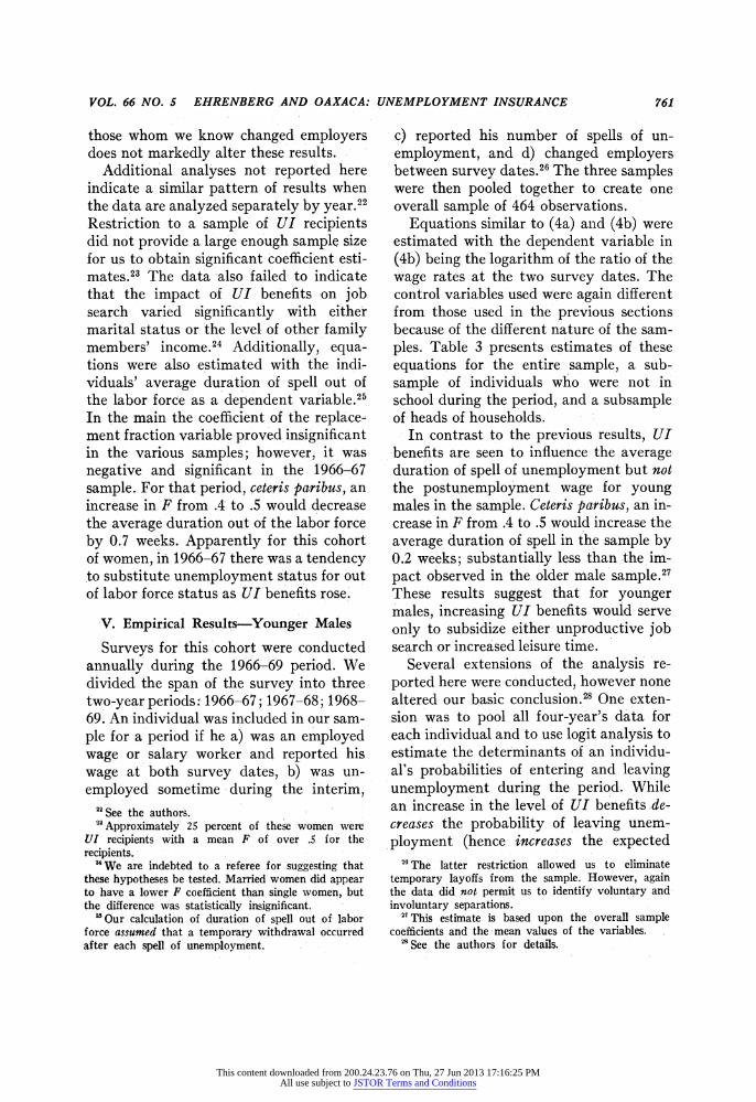
c) reported his number of spells of unemployment, and d) changed employers between survey dates.26 The three samples were then pooled together to create one overall sample of 464 observations.

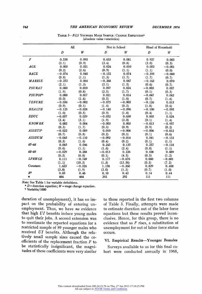
Equations similar to (4a) and (4b) were estimated with the dependent variable in (4b) being the logarithm of the ratio of the wage rates at the two survey dates. The control variables'used were again different from those -used in the previous sections because of the different nature of the samples. Table 3 presents estimates of these equations for the entire sample, a subsample of individuals who were not in school during the period, and a subsample of heads of households.

In contrast to the previous results, UI benefits are seen to influence the average duration of spell of unemployment but not the postunemployment wage for young males in the sample. Ceteris paribus, an increase in F from .4 to .5 would increase the average duration of spell in the sample by 0.2 weeks; substantially less than the impact observed in the older male sample.27 These results suggest that for younger males, increasing UI benefits would serve only to subsidize either unproductive job search or increased leisure time.

Several extensions of the analysis' reported here were conducted, however none altered our basic conclusion.28 One extension was to pool all four-year's data for each individual and to use logit analysis to estimate the determinants of an individual's probabilities of entering and leaving unemployment during the period. While an increase in the level of UI benefits decreases the probability of leaving unemployment (hence increases the expected

VOL. 66 NO. 5 EHRENBERG.AND OAXACA: UNEMPLOYMENT INSURANCE 761

those whom we know changed employers does not markedly alter these results.

Additional analyses not reported here indicate a similar pattern of results when the data are analyzed separately by year.22 Restriction to a sample of UI recipients did not provide a large enough sample size for us to obtain significant coefficient estimates.23 The-data also failed to indicate that the impact of UI benefits on job search varied significantly with either marital status or the level of other family members' income.24 Additionally, equations were also estimated with the individuals' average duration of spell out of the labor force as a dependent variable.25 In the main the coefficient of the replacement fraction variable proved insignificant in the various samples; however, it was negative and'significant in the 1966-67 sample. For that period, ceteris paribus, an increase in F from .4 to .5 would decrease the average duration out of the labor force by 0.7 weeks. Apparently for this cohort of women, in 1966-67 there was a tendency to substitute unemployment status for out of labor force status as UI benefits rose.

V. Empirical Results-Younger Males

Surveys for this'cohort were conducted annually during the 1966-69 period. We divided the span of the survey into three two-year periods: 1966-67; 1967-68; 1968- 69. An individual was included in our sample for a period if he a) was an employed wage or salary worker and reported his wage at both survey dates, b) was unemployed sometime during the interim,

22 See the authors. Approximately 25 percent of these women were

UI recipients with a mean F of over .5 for the recipients.

' We are indebted to a referee for suggesting that these hypotheses be tested. Married women did appear to have a lower F coefficient than single women, but the difference was statistically insignificant.

25Our calculation of duration of spell out of labor force assumed that a temporary withdrawal occurred after each spell of unemployment.

26 The latter restriction. allowed us to eliminate temporary layoffs from. the sample. However, again the data did not permit us to identify voluntary and involuntary separations.

2T This estimate is based upon the overall sample coefficients and the mean values of the variables.

2 See the authors for details.




TABLE 3-NLS YOUNGER MALE SAMPLE: CHANGE EMPLOYERSB (absolute value t-statistics)

All: Not in School Head of Household

D W D W D W

F 0.538 0.093 0.653 0.081 0.927 0.085 (-2.1) (0.9) (2.4) (0.8) (2.0) (0.5)

AGE 0.003 0.021 0.024 0.010 0.052 -0.001 (0.2) (2.6) (0.9) (1.1) (1.1) (0.0)

RACE -0.074 0.040 -0.152 0.074 -0.395 -0.060 (0.8) (1.1) (1.3) (1.7) (1.7) (0. 7)

MARRIE -0.252 0.064 -0.268 0.067 -0.163 0.070 (2.1) (1.3) (2.1) (1.5) (0.6) (0.7)

PSURAT 0.060 0.010 0.097 0.024 -0.003 0.007 (1.9) (0.8) (2.5) (1.7) (0.1) (0.3)

pSUPOPb 0.000 0.017 0.021 0.014 -0 .047 0.042 (0.0) (1.4) (0.5) (1.0) (0.7) (1.6)

TENURE -0.036 -0.002 -0.075 -0.005 -0.126 0.015 (0.9) (0.1) (1.4) (0.3) (1.8) (0.6)

HEALTH -0.125 --0.028 -0.140 -0.096 -0.100 -0.095 -(1.0) (0.5) (0.9) (1.8) (0.4) (1.1)

EDUC -0.057 0.029 -0.052 0.030 0.005 0.024 (2.4) (3.1) (1.9) (3.0) (0.1) (1.4)

KNOWRK 0.002 0.004 -0.003 0.003 -0.013 -0.957 (0.3) (1.7) (0.3) (0.9) (0.9) (0.2)

ASSETSb -0. 022 0.009 0.010 -0.006 -0.006 -0.012 (0.7) (0.8) (0.2) (0.3) (0.1) (0.6)

ASSDUM -0.045 -0.110 -0.092 -0.014 0.041 -0.132 (0.3) (1.6) (0.4) (0.2) (0.1) (1.1)

67-68 0.065 0.046 0.243 0.135 0.257 -0.118 (0.6) (1.1) (1.6) (2.4) (0.8) (1.1)

68-69 -0.029 0.288 -0.013 0.226 0.108 0.089 (0.3) (6.8) (0.1) (4.5) (0.5) (1.2)

LPRWGE 0.111 -0.749 0.177 -0.676 0.060 -0.-601 (1.1) (18.3) (1.3) (13.56) (0.3) (7.2)

Constant 1.625 -0.326 1.158 -0.260 0.829 0.408 (3.8) (1.9) (2.0) (1.3) (0.7) (1.0)

D2 0.05 0.46 0.10 0.42 0.14 0.44 n 464 464 292 292 111 111

Note: See Table 1 for variable definitions. D=duration equation; W=wage change equation.

b Variable/1000

duration:of unemployment), it has no impact on the probability of entering unemployment. Thus, we have no evidence that high UI benefits induce young males to quit their jobs. A second extension was to reestimate the reported equations for a restricted sample of 89 younger males who received UI benefits. Although the rela- tively small sample sizes caused the coefficients of the replacement fraction F to be statistically insignificant, the magnitudes of these coefficients were very similar

to those reported in the first two columns of Table 3. Finally, attempts were made to estimate duration out of the labor force equations but these results. proved incon- clusive. Hence, for this group, there -is no evidence that as F rises, a substitution of unemployment for out of labor force status occurs.

VI. Empirical Results-Younger Females

Surveys available to us for this final cohort were conducted annually in 1968,




TABLE 4-NLS YOUNGER FEMALE SAPLEB (absolute value t-statistics)

Self or Spouse All Not in'School Head of Household

D W 0 D W 0 D W 0

F 1.222 0.041 -8.002 1.221 0.039 -8.379 1.499 -0.053 -7.075 (3.8) (0.4) (2.1) (3.8) (0.4) (2.2) (3.6) (0.4) (1.6)

AGE 0.027 0.012 -1.046 0.038 -0.001 -0.991 0.021 0.008 -0.685 (1.3) (1.9) (4.5) (1.7) (0.2) (3.8) '(0.7) (0.8) (2.2)

RACE -0.206 0.034 0.702 -0.226 0.056 0.639 -0.218 0.037 2.889 (2.2) (1.1) (0.7) (2.3) (1.8) (0.6) (1.5) (0.8) (1.9)

MARRIE 0.036 -0.007 0.064 0.017 -0.031 0.182 0. 144 -0.033 1.456 (0.3) (0.1) (0.0) (0.1) (0.7) (0.1) (0.8) (0.6) (0.8)

PSURAT 0.007 0.005 -0.268 -0.005 0.003 '-0.143 0.013 0.011 -0.522 (0.3) (0.6) (1.0) (0.2) (0.4) (0.5) (0.4) (1.1) (1.6)

PSUPOPb -0.788 0.607 1.744 --0.849 0.570 0.546 -0.399 0.744 5.174 (2.2) (5.1) (0.4) (2.1) (4.5) (0.1) (0.7) (4.2) (0.8)'

FEMDEM -0.004- -0.008 0.146 -0.007 -0.008 0.170 -0.023 -0.011 0.253 (0.4) (2.2) (1.2) (0.6) (2.3) (1.3) (1.3) (2.1) (1.4)

HEALTH -0.033 -0.057 5.518 0.023 -0.083 5.590 0.116 0.082 2.436 (0.2) (0.9) (2.2) (0.1) (1.2) (2.2) (0.4) (0.9) (0.8)

LPRWGE -0.110 -0.707 -0.486 -0.124 -0.725 -0.098 -0.013 -0.711 -0.588 -(1.5) (28.9) (0.6) (1.4) (25.9) (0.1) (0.1) (19.8) (0.5)

HUSBYb -0.433 0.035 2.800 -0.326 0.052 2.197 -0.529 0.014 3.212 (1.8) (0.4) (1.0) (1.3) (0.7) (0.8) (2.0) (0.2) (1.2)

DEPEND 0.010 -0.002 0.857- 0.121 0.004 0.951 0.144 -0.011 1.060 (1.8) (0.1) (1.4) (2.1) (0.2) (1.4) (2.3) (0.6) (1.6)

EDUC 0.007 -0.054 0.434 0.014 0.046 0.665 0.017 0.042 0.771 (0.3) (6.6) (1.5) (0.5) (5.4) (2.1) (0.5) (4.0) (2.2)

KNOWRK -0.015 0.005 0.016 -0.015 0.010 -0.096 -0.017 aO.914 -0.767 (0.7) (0.8) (0.1) (0.6) (1.3) (0.3) (0.5) (0.0) (2.2)

ASSETSb -0.092 0.014 -0.746' '-0.082 0.021 -0.716 -0.022 0.032 -0.520 (0.5) (0.2) (0.3) (0.4) (0.4) (0.3) (0.1) (0 5) (0.3)

NASSDM -0.215 -0.020 2.670 -0.304 -0.022 0.191 -0.240 -0.043 3.741 (1.4) (0.4) (1.6) (1.8) (0.4) (1.0) (1.1) (0.6) (1.6)

67-68 .698 -0.096 7.772 0.726 -0.083 7.733 0.681 -0.097 6.873 (7.1) (3.0) (6.9) (6.8) (2.5) (6.3) (5.0) (2.3) (4.8)

68-69 0.540 -0.046 0.574 0.488 -0.013 0.970 0.571 -0.013 -1.051 (5.0) (1.3) (0.5) (4.3), (0.4) (0.7) (3.9) (0.3) (0-.7)

Constant 0.521 -0.249 12.501 0.417 0.129 8.811 0.940 0.168 0.227 (1.0). (1.4) (2.0) (0.7) (0.7) (1.2) (1.1) (0.7) (0.0)

R2 - .17 .60 -.19 .19 .60 .18 .21 .61 .20 n 613 613 613 507 507 507 -293 293 293

Note: See Table 1 for variable definitions. a D = duration equation; W = wage change equation; 0 duration out of labor force equation. b Variable/1000.

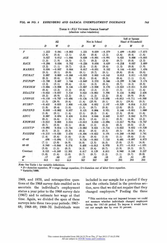
1969, and 1970, and retrospective questions at the 1968 survey date enabled us to ascertain the individual's employment status a year prior to the 1968 survey date (1967) and to estimate her wage at that time. Again, we divided the span of these surveys into three two-year periods: 1967- 68; 1968-69; 1969-70. Individuals were

included in our sample for a period if they met the criteria listed in the previous section, save that we did not require that they changed employers.29 Pooling the three

9 This restriction was not imposed because we could not measure whether individuals changed 'employers during the 1967-68 period. To impose it would have cut our sample size by over 50 percent.




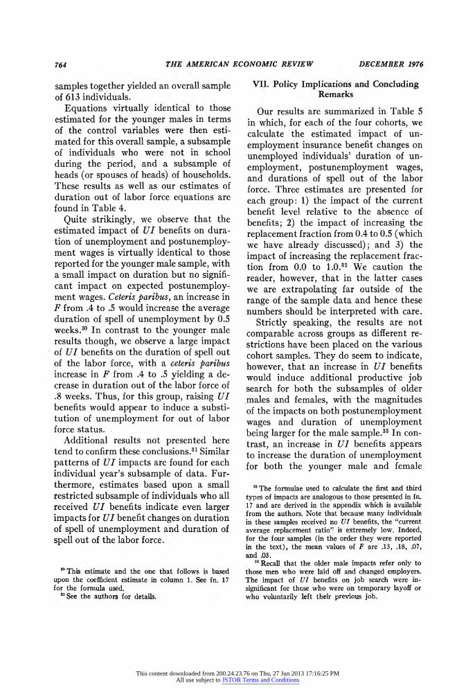
samples together yielded an overall sample of 613 individuals.

Equations virtually identical to those estimated for the younger males in terms of the control variables were then estimated for this overall sample, a subsample of individuals who were not in school during the period, and a subsample of heads (or spouses of heads) of households. These results as well as our estimates of duration out of labor force equations are found in Table 4.

Quite strikingly, we observe that the estimated impact of UI benefits on duration of unemployment and postunemployment wages.is virtually identical to those reported for the younger male sample, with a small impact on duration but no significant impact on expected postunemployment wages. Ceteris paribus, an increase in F from .4 to .5 would increase the average duration of, spell of unemployment by 0.5 weeks.30 In contrast to the younger male results though, we observe' a large impact of UI benefits on the duration of spell out of the labor force, with a ceteris paribus increase in F from .4 to .5 yielding a decrease in duration out of the labor force of .8 weeks. Thus, for this group, raising UI benefits would appear to induce a substitution of unemployment for out of labor force status.

Additional results not presented here tend to confirm these conclusions.31 Similar patterns of UI impacts are found for each individual year's' subsample of data. Fur- thermore, estimates based upon a small restricted subsample of individuals who all received UI benefits indicate even larger impacts for UI benefit changes on duration of spell of unemployment and duration of spell out. of the labor force.

VII. Policy Implications and Concluding Remarks

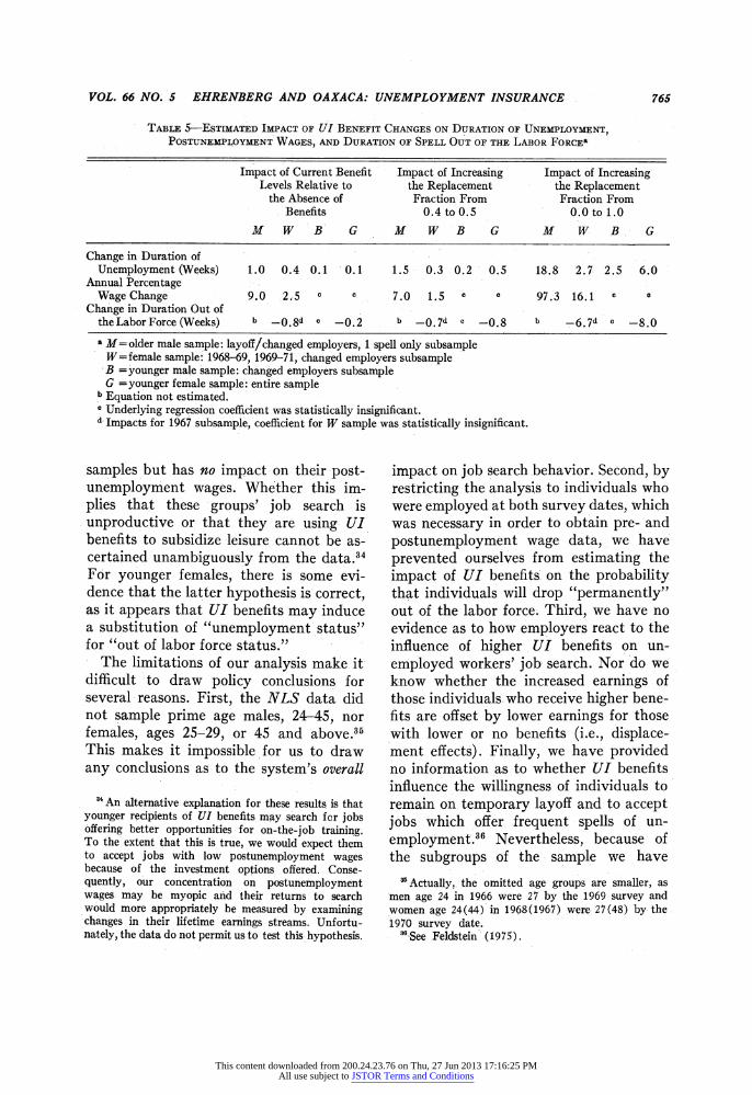
Our results are summarized in Table 5 in which, for' each of the four cohorts, we calculate the estimated impact of unemployment insurance benefit changes on unemployed individuals' duration of unemployment, postunemployment wages, and durations of spell out of the labor force. Three estimates are presented for each group: 1) the impact of the current benefit level relative to the absence of benefits; 2) the impact of increasing the replacement fraction from 0.4 to 0.5 (which. we have already discussed); and 3) the impact of increasing the replacement fraction from 0.0 to 1.0.32 We caution the reader, however, that in the latter cases we are extrapolating far outside of the range of the sample data and hence these numbers should be interpreted with care.

Strictly, speaking, the results are not comparable across groups as different re- strictions have been placed on the various 'cohort samples. They do seem to indicate, however, that an increase in UI benefits would induce additional productive job search for both the subsamples of older males 'and females, with the, magnitudes of the impacts on both postunemployment wages and duration of unemployment being larger for the male sample.33 In contrast, an increase in UI benefits appears to increase the duration of unemployment for both the younger male and female

30This estimate and .the one that follows is based upon the coefficient estimate in column 1. See fn. 17 for the formula used.

"See the authors for details.

2The formulae used to calculate the first and third types of impacts are analogous to those presented in fn. 17 and are derived in the appendix which is available from the authors. Note that because many individuals in these samples received no UI benefits, the "current average replacement ratio" is extremely low. Indeed, for the four samples (in the order they were reported in the text), the mean values of F are' .13, .18, .07, and .03.

33 Recall that the older male impacts refer only to those men who were laid off and changed employers. The impact of UI benefits on job search were 'insignificant for those who were on temporary layoff or who voluntarily left their previous job.




TABLE 5-ESTIMATED IMPACT OF UI BENEFIT CHANGES ON DURATION OF UNEMPLOYMENT, POSTUNEMPLOYMENT WAGES, AND DURATION OF SPELL OUT OF THE LABOR FORCEa

Impact of Current Benefit Impact of Increasing Impact of Increasing Levels Relative to the Replacement the Replacement

the Absence of Fraction From Fraction From Benefits 0.4 to 0.5 0.0 to 1.0

M W B G M W B G M W B G

Change in Duration of Unemployment (Weeks) 1.0 0.4 0.1 0.1 1.5 0.3 0.2 0.5 18.8 2.7 2.5 6.0

Annual Percentage Wage Change 9.0 2.5 C C 7.0 1.5 C 0 97.3 16.1 0 o

Change in Duration Out of theLabor Force (Weeks) b -0.8d c -0.2 b -0.7d -0.8 b -6. 7d

a M =older male sample: layoff/changed employers, 1 spell only subsample W=female sample: 1968-69, 1969-71, changed employers subsample B =younger male sample: changed employers subsample G =younger female sample: entire sample

b Equation not estimated. U Underlying regression coeffcient was statistically insignificant.

d Impacts for 1967 subsample, coefficient for W sample was statistically insignificant.

samples but has no impact on their postunemployment wages. Whether this implies that these groups' job search is unproductive or that they are using UI benefits to subsidize leisure cannot be ascertained unambiguously from the data.34 For younger females, there is some evidence that the latter hypothesis is correct, as it appears that UI benefits may induce a substitution of "unemployment status" for "out of labor force status."

The limitations of our analysis make it difficult to draw policy conclusions for several reasons. First, the NLS data did not sample prime age males, 24-45, nor females, ages 25-29, or 45 and above.35 This makes it impossible for us to draw any conclusions as to the system's overall

impact on job search behavior. Second, by restricting the analysis to individuals who were employed at both survey dates, which was necessary in order to obtain pre- and postunemployment wage data, we have prevented ourselves from estimating the impact of UI benefits: on the probability that individuals will drop "permanently" out of the labor force. Third, we have no evidence as to how employers react to the influence of higher UI benefits on unemployed workers' job search. Nor do we know whether the increased earnings of those individuals. who receive higher benefits are offset by lower earnings for those with lower or no benefits (i.e., displace- ment effects). Finally, we have provided no information as to whether UI benefits influence the willingness of individuals to remain on temporary layoff and to accept jobs which offer frequent spells of unemployment.36 Nevertheless, because of the subgroups of the sample we have

"4 An alternative explanation for these results is that younger recipients of UI benefits may search for jobs offering better opportunities for on-the-job training. To the extent that this is true, we would expect them to accept jobs with low postunemployment wages because of the investment options offered. Conse- quently, our concentration on postunemployment wages may be myopic and their returns to search would more appropriately be measured by examining changes in their lifetime earnings streams. Unfortu- nately, the data do not permit us to test this hypothesis.

35Actually,. the omitted age groups are smaller, as men age 24 in 1966 were 27 by the 1969 survey and women age 24(44) in 1968(1967) were 27(48) by the 1970 survey date.

36See Feldstein (1975).




found that apparently would not engage in additional productive job search, it is unlikely that one could justify raising. Ul benefit levels on efficiency grounds. Rather, equity and income maintenance considera- tions would appear to be the necessary basis for such actions.3"

See Feldstein (1974) and Gary Fields for discus- sions relating to equity and income maintenance con- siderations and the current impact of the UI, system on the personal distribution of income.

REFERENCES

K. Burdett, "Theories of Search in a Labor Market," techn. anal. pap. no. 13, Office of Evaluation, ASPER, U.S. Department of Labor, Washington 1973.

G. Chapin, "Unemployment Insurance, Job Search and the Demand for Leisure," West- ern Econ. J., Mar. 1971, 9, 102-07.

K. Classen, "The Effects -of Unemployment Insurance: Evidence From Pennsylvania,"

- mimeo, Apr. 1975. R. Ehrenberg, "Job Search, Duration of Un-

employment, and Subsequent Wage Gain: A Benefit-Cost Analysis," mimeo, Oct. 1974.

,"An Evaluation of the Adequacy of Existing Data Sources for Research on the Unemployment Insurance System and Re- flections on Proposed New Data Collection Efforts," paper prepared for the U.S. De- partment of Labor, mimeo, Aug. 1975.

- ,and R. Oaxaca, "The Economic Ef- fects of Unemployment Insurance Benefits

on Unemployed Workers Job Search," final report submitted to the U.S. Department of Labor Contract L 74-49, July 1976.

M. Feldstein, "The Economics of the New Unemployment," Publ. Interest, Fall 1973, 33, 3-42.

"Unemployment Compensation, Ad- verse Incentives and Distributional Anom- alies," Nat. Tax J., June 1974, 37, 213-44.

,"Temporary Layoffs in the Theory of Unemployment," Harvard Inst. Econ. Res. disc. pap., June 1975.

G. Fields, "The Direct Labor Market Effects of the U.S. Unemployment Insurance Sys- tem: A Review of Recent Evidence," techn. anal. pap. no. 26, Office of Evalua- tion, ASPER, U.S. Department of Labor, Washington Jan. 1975.

W. Haber and M. Murray, Unemployment Insurance in the American Economy, Home- wood 1966.

S. Marston, "The Impact of Unemployment Insurance on Job Search," Brookings Papers, Washington 1975, 1, 13-60.

D. Mortensen, "Job Search, the Duration of Unemployment, and the Phillips Curve," Amer. Econ. Rev., Dec. 1970, 60, 847-62.

H. Parnes, "The National Longitudinal Sur- -veys: New Vistas for Labor Market Re- search," Amer. Econ. Rev. Proc., May 1975, 65, 244-49.

R. Schmidt, "The Theory of -Search and the Duration of Unemployment," mimeo, Aug. 1973.

Center for Human Resource Research, Na- tional Longitudinal Survey Handbook, Co- lumbus, Dec. 1973.



Documents

P) Ehrenberg-Oaxaca_1976_Unemployment insurance duration of unemployment.pdf