P A G E S 2 1 6 T O 2 3 1 O F h ttp ://w w w .c se .iitb ...cs709/notes/enotes/basicsOfUnivariate... · ... in te rsp e rse d w ith p a g e s b e tw e e n 2 3 9 a n d 2 5 3 a n d

PAGES 216 TO 231 OF ht tp://www.cse.iitb.ac.in/~ cs709/notes/BasicsOfConvexOpt imizat ion.pdf, interspersed with pages between 239 and 253 and summary of material thereafter, which extend univariate concepts to generic spaces

ppp

Convex Optimization — Boyd & Vandenberghe

3. Convex functions

• basic properties and examples

• operations that preserve convexity

• the conjugate function

• quasiconvex functions

• log-concave and log-convex functions

• convexity with respect to generalized inequalities

3–1

Definition

f : Rn → R is convex if dom f is a convex set and

f(θx + (1 − θ)y) ≤ θf(x) + (1 − θ)f(y)

for all x, y ∈ dom f , 0 ≤ θ ≤ 1

(x, f(x))

(y, f(y))

• f is concave if −f is convex

• f is strictly convex if dom f is convex and

f(θx + (1 − θ)y) < θf(x) + (1 − θ)f(y)

for x, y ∈ dom f , x 6= y, 0 < θ < 1

Convex functions 3–2

First-order condition

f is differentiable if dom f is open and the gradient

∇f(x) =

(

∂f(x)

∂x1,∂f(x)

∂x2, . . . ,

∂f(x)

∂xn

)

exists at each x ∈ dom f

1st-order condition: differentiable f with convex domain is convex iff

f(y) ≥ f(x) + ∇f(x)T (y − x) for all x, y ∈ dom f

(x, f(x))

f(y)

f(x) + ∇f(x)T (y − x)

first-order approximation of f is global underestimator


Second-order conditions

f is twice differentiable if dom f is open and the Hessian ∇2f(x) ∈ Sn,

∇2f(x)ij =∂2f(x)

∂xi∂xj, i, j = 1, . . . , n,

exists at each x ∈ dom f

2nd-order conditions: for twice differentiable f with convex domain

• f is convex if and only if

∇2f(x) � 0 for all x ∈ dom f

• if ∇2f(x) ≻ 0 for all x ∈ dom f , then f is strictly convex


Examples on R

convex:

• affine: ax + b on R, for any a, b ∈ R

• exponential: eax, for any a ∈ R

• powers: xα on R++, for α ≥ 1 or α ≤ 0

• powers of absolute value: |x|p on R, for p ≥ 1

• negative entropy: x log x on R++

concave:

• affine: ax + b on R, for any a, b ∈ R

• powers: xα on R++, for 0 ≤ α ≤ 1

• logarithm: log x on R++


Examples on Rn and Rm×n

affine functions are convex and concave; all norms are convex

examples on Rn

• affine function f(x) = aTx + b

• norms: ‖x‖p = (∑n

i=1 |xi|p)1/p for p ≥ 1; ‖x‖∞ = maxk |xk|

examples on Rm×n (m × n matrices)

• affine function

f(X) = tr(ATX) + b =

m∑

i=1

n∑

j=1

AijXij + b

• spectral (maximum singular value) norm

f(X) = ‖X‖2 = σmax(X) = (λmax(XTX))1/2


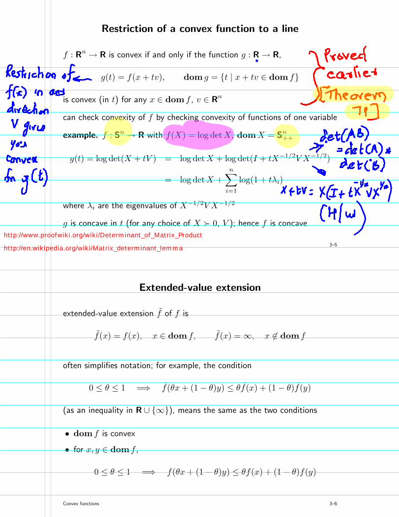
Restriction of a convex function to a line

f : Rn → R is convex if and only if the function g : R → R,

g(t) = f(x + tv), dom g = {t | x + tv ∈ dom f}

is convex (in t) for any x ∈ dom f , v ∈ Rn

can check convexity of f by checking convexity of functions of one variable

example. f : Sn → R with f(X) = log detX, domX = Sn++

g(t) = log det(X + tV ) = log detX + log det(I + tX−1/2V X−1/2)

= log detX +

n∑

i=1

log(1 + tλi)

where λi are the eigenvalues of X−1/2V X−1/2

g is concave in t (for any choice of X ≻ 0, V ); hence f is concave


Extended-value extension

extended-value extension f̃ of f is

f̃(x) = f(x), x ∈ dom f, f̃(x) = ∞, x 6∈ dom f

often simplifies notation; for example, the condition

0 ≤ θ ≤ 1 =⇒ f̃(θx + (1 − θ)y) ≤ θf̃(x) + (1 − θ)f̃(y)

(as an inequality in R ∪ {∞}), means the same as the two conditions

• dom f is convex

• for x, y ∈ dom f ,

0 ≤ θ ≤ 1 =⇒ f(θx + (1 − θ)y) ≤ θf(x) + (1 − θ)f(y)


ht tp://www.proofwiki.org/wik i/Determ inant_of_Mat rix_Product

ht tp://en.wik ipedia.org/wik i/Mat rix_determ inant_lem m a

Examples

quadratic function: f(x) = (1/2)xTPx + qTx + r (with P ∈ Sn)

∇f(x) = Px + q, ∇2f(x) = P

convex if P � 0

least-squares objective: f(x) = ‖Ax − b‖22

∇f(x) = 2AT (Ax − b), ∇2f(x) = 2ATA

convex (for any A)

quadratic-over-linear: f(x, y) = x2/y

∇2f(x, y) =2

y3

[

y−x

] [

y−x

]T

� 0

convex for y > 0 xy

f(x

,y)

−2

0

2

0

1

20

1

2


log-sum-exp: f(x) = log∑n

k=1 expxk is convex

∇2f(x) =1

1Tzdiag(z) − 1

(1Tz)2zzT (zk = exp xk)

to show ∇2f(x) � 0, we must verify that vT∇2f(x)v ≥ 0 for all v:

vT∇2f(x)v =(∑

k zkv2k)(

∑

k zk) − (∑

k vkzk)2

(∑

k zk)2≥ 0

since (∑

k vkzk)2 ≤ (

∑

k zkv2k)(

∑

k zk) (from Cauchy-Schwarz inequality)

geometric mean: f(x) = (∏n

k=1 xk)1/n on Rn

++ is concave

(similar proof as for log-sum-exp)


> > 3*(sin(0.5+ 0.25*3*-3)).*cos(-3)ans = 2.9224

> > 3*(sin(0.5+ 0.25*2*-3)).*cos(-3)ans = 2.4991

ht tp://www.cse.iitb.ac.in/~ CS709/notes/code/unconst rainedOpt /GraphicalSolut ion_Example6_1a.m

if

Epigraph and sublevel set

α-sublevel set of f : Rn → R:

Cα = {x ∈ dom f | f(x) ≤ α}

sublevel sets of convex functions are convex (converse is false)

epigraph of f : Rn → R:

epi f = {(x, t) ∈ Rn+1 | x ∈ dom f, f(x) ≤ t}

epi f

f

f is convex if and only if epi f is a convex set


Jensen’s inequality

basic inequality: if f is convex, then for 0 ≤ θ ≤ 1,

f(θx + (1 − θ)y) ≤ θf(x) + (1 − θ)f(y)

extension: if f is convex, then

f(E z) ≤ E f(z)

for any random variable z

basic inequality is special case with discrete distribution

prob(z = x) = θ, prob(z = y) = 1 − θ


Operations that preserve convexity

practical methods for establishing convexity of a function

1. verify definition (often simplified by restricting to a line)

2. for twice differentiable functions, show ∇2f(x) � 0

3. show that f is obtained from simple convex functions by operationsthat preserve convexity

• nonnegative weighted sum• composition with affine function• pointwise maximum and supremum• composition• minimization• perspective


Positive weighted sum & composition with affine function

nonnegative multiple: αf is convex if f is convex, α ≥ 0

sum: f1 + f2 convex if f1, f2 convex (extends to infinite sums, integrals)

composition with affine function: f(Ax + b) is convex if f is convex

examples

• log barrier for linear inequalities

f(x) = −m

∑

i=1

log(bi − aTi x), dom f = {x | aT

i x < bi, i = 1, . . . ,m}

• (any) norm of affine function: f(x) = ‖Ax + b‖


Pointwise maximum

if f1, . . . , fm are convex, then f(x) = max{f1(x), . . . , fm(x)} is convex

examples

• piecewise-linear function: f(x) = maxi=1,...,m(aTi x + bi) is convex

• sum of r largest components of x ∈ Rn:

f(x) = x[1] + x[2] + · · · + x[r]

is convex (x[i] is ith largest component of x)

proof:

f(x) = max{xi1 + xi2 + · · · + xir | 1 ≤ i1 < i2 < · · · < ir ≤ n}


Pointwise supremum

if f(x, y) is convex in x for each y ∈ A, then

g(x) = supy∈A

f(x, y)

is convex

examples

• support function of a set C: SC(x) = supy∈C yTx is convex

• distance to farthest point in a set C:

f(x) = supy∈C

‖x − y‖

• maximum eigenvalue of symmetric matrix: for X ∈ Sn,

λmax(X) = sup‖y‖2=1

yTXy


Composition with scalar functions

composition of g : Rn → R and h : R → R:

f(x) = h(g(x))

f is convex ifg convex, h convex, h̃ nondecreasing

g concave, h convex, h̃ nonincreasing

• proof (for n = 1, differentiable g, h)

f ′′(x) = h′′(g(x))g′(x)2 + h′(g(x))g′′(x)

• note: monotonicity must hold for extended-value extension h̃

examples

• exp g(x) is convex if g is convex

• 1/g(x) is convex if g is concave and positive


Vector composition

composition of g : Rn → Rk and h : Rk → R:

f(x) = h(g(x)) = h(g1(x), g2(x), . . . , gk(x))

f is convex ifgi convex, h convex, h̃ nondecreasing in each argument

gi concave, h convex, h̃ nonincreasing in each argument

proof (for n = 1, differentiable g, h)

f ′′(x) = g′(x)T∇2h(g(x))g′(x) + ∇h(g(x))Tg′′(x)

examples

•∑m

i=1 log gi(x) is concave if gi are concave and positive

• log∑m

i=1 exp gi(x) is convex if gi are convex


Minimization

if f(x, y) is convex in (x, y) and C is a convex set, then

g(x) = infy∈C

f(x, y)

is convex

examples

• f(x, y) = xTAx + 2xTBy + yTCy with

[

A BBT C

]

� 0, C ≻ 0

minimizing over y gives g(x) = infy f(x, y) = xT (A − BC−1BT )x

g is convex, hence Schur complement A − BC−1BT � 0

• distance to a set: dist(x, S) = infy∈S ‖x − y‖ is convex if S is convex


Perspective

the perspective of a function f : Rn → R is the function g : Rn ×R → R,

g(x, t) = tf(x/t), dom g = {(x, t) | x/t ∈ dom f, t > 0}

g is convex if f is convex

examples

• f(x) = xTx is convex; hence g(x, t) = xTx/t is convex for t > 0

• negative logarithm f(x) = − log x is convex; hence relative entropyg(x, t) = t log t − t log x is convex on R2

++

• if f is convex, then

g(x) = (cTx + d)f(

(Ax + b)/(cTx + d))

is convex on {x | cTx + d > 0, (Ax + b)/(cTx + d) ∈ dom f}


Subgradients

• subgradients

• strong and weak subgradient calculus

• optimality conditions via subgradients

• directional derivatives

Prof. S. Boyd, EE364b, Stanford University

Basic inequality

recall basic inequality for convex differentiable f :

f(y) ≥ f(x) +∇f(x)T (y − x)

• first-order approximation of f at x is global underestimator

• (∇f(x),−1) supports epi f at (x, f(x))

what if f is not differentiable?

Prof. S. Boyd, EE364b, Stanford University 1

Subgradient of a function

g is a subgradient of f (not necessarily convex) at x if

f(y) ≥ f(x) + gT (y − x) for all y

x1 x2

f(x1) + gT1 (x − x1)

f(x2) + gT2 (x − x2)

f(x2) + gT3 (x − x2)

f(x)

g2, g3 are subgradients at x2; g1 is a subgradient at x1


• g is a subgradient of f at x iff (g,−1) supports epi f at (x, f(x))

• g is a subgradient iff f(x) + gT (y − x) is a global (affine)underestimator of f

• if f is convex and differentiable, ∇f(x) is a subgradient of f at x

subgradients come up in several contexts:

• algorithms for nondifferentiable convex optimization

• convex analysis, e.g., optimality conditions, duality for nondifferentiableproblems

(if f(y) ≤ f(x) + gT (y − x) for all y, then g is a supergradient)


Example

f = max{f1, f2}, with f1, f2 convex and differentiable

x0

f1(x)f2(x)

f(x)

• f1(x0) > f2(x0): unique subgradient g = ∇f1(x0)

• f2(x0) > f1(x0): unique subgradient g = ∇f2(x0)

• f1(x0) = f2(x0): subgradients form a line segment [∇f1(x0),∇f2(x0)]


Subdifferential

• set of all subgradients of f at x is called the subdifferential of f at x,denoted ∂f(x)

• ∂f(x) is a closed convex set (can be empty)

if f is convex,

• ∂f(x) is nonempty, for x ∈ relint dom f

• ∂f(x) = {∇f(x)}, if f is differentiable at x

• if ∂f(x) = {g}, then f is differentiable at x and g = ∇f(x)


Example

f(x) = |x|

f(x) = |x| ∂f(x)

x

x

1

−1

righthand plot shows⋃

{(x, g) | x ∈ R, g ∈ ∂f(x)}


Subgradient calculus

• weak subgradient calculus: formulas for finding one subgradientg ∈ ∂f(x)

• strong subgradient calculus: formulas for finding the wholesubdifferential ∂f(x), i.e., all subgradients of f at x

• many algorithms for nondifferentiable convex optimization require onlyone subgradient at each step, so weak calculus suffices

• some algorithms, optimality conditions, etc., need whole subdifferential

• roughly speaking: if you can compute f(x), you can usually compute ag ∈ ∂f(x)

• we’ll assume that f is convex, and x ∈ relint dom f


Some basic rules

• ∂f(x) = {∇f(x)} if f is differentiable at x

• scaling: ∂(αf) = α∂f (if α > 0)

• addition: ∂(f1 + f2) = ∂f1 + ∂f2 (RHS is addition of sets)

• affine transformation of variables: if g(x) = f(Ax+ b), then∂g(x) = AT∂f(Ax+ b)

• finite pointwise maximum: if f = maxi=1,...,m

fi, then

∂f(x) = Co⋃

{∂fi(x) | fi(x) = f(x)},

i.e., convex hull of union of subdifferentials of ‘active’ functions at x


f(x) = max{f1(x), . . . , fm(x)}, with f1, . . . , fm differentiable

∂f(x) = Co{∇fi(x) | fi(x) = f(x)}

example: f(x) = ‖x‖1 = max{sTx | si ∈ {−1, 1}}

1

1

−1

−1

∂f(x) at x = (0, 0)

1

1

−1

at x = (1, 0)

(1,1)

at x = (1, 1)


Pointwise supremum

if f = supα∈A

fα,

clCo⋃

{∂fβ(x) | fβ(x) = f(x)} ⊆ ∂f(x)

(usually get equality, but requires some technical conditions to hold, e.g.,A compact, fα cts in x and α)

roughly speaking, ∂f(x) is closure of convex hull of union ofsubdifferentials of active functions


Weak rule for pointwise supremum

f = supα∈A

fα

• find any β for which fβ(x) = f(x) (assuming supremum is achieved)

• choose any g ∈ ∂fβ(x)

• then, g ∈ ∂f(x)


example

f(x) = λmax(A(x)) = sup‖y‖2=1

yTA(x)y

where A(x) = A0 + x1A1 + · · ·+ xnAn, Ai ∈ Sk

• f is pointwise supremum of gy(x) = yTA(x)y over ‖y‖2 = 1

• gy is affine in x, with ∇gy(x) = (yTA1y, . . . , yTAny)

• hence, ∂f(x) ⊇ Co {∇gy | A(x)y = λmax(A(x))y, ‖y‖2 = 1}(in fact equality holds here)

to find one subgradient at x, can choose any unit eigenvector y associatedwith λmax(A(x)); then

(yTA1y, . . . , yTAny) ∈ ∂f(x)


Expectation

• f(x) = E f(x, u), with f convex in x for each u, u a random variable

• for each u, choose any gu ∈ ∂f(x, u) (so u 7→ gu is a function)

• then, g = E gu ∈ ∂f(x)

Monte Carlo method for (approximately) computing f(x) and a g ∈ ∂f(x):

• generate independent samples u1, . . . , uK from distribution of u

• f(x) ≈ (1/K)∑K

i=1 f(x, ui)

• for each i choose gi ∈ ∂xf(x, ui)

• g = (1/K)∑K

i=1 gi is an (approximate) subgradient(more on this later)


Minimization

define g(y) as the optimal value of

minimize f0(x)subject to fi(x) ≤ yi, i = 1, . . . ,m

(fi convex; variable x)

with λ⋆ an optimal dual variable, we have

g(z) ≥ g(y)−m∑

i=1

λ⋆i (zi − yi)

i.e., −λ⋆ is a subgradient of g at y


Composition

• f(x) = h(f1(x), . . . , fk(x)), with h convex nondecreasing, fi convex

• find q ∈ ∂h(f1(x), . . . , fk(x)), gi ∈ ∂fi(x)

• then, g = q1g1 + · · ·+ qkgk ∈ ∂f(x)

• reduces to standard formula for differentiable h, fi

proof:

f(y) = h(f1(y), . . . , fk(y))

≥ h(f1(x) + gT1 (y − x), . . . , fk(x) + gTk (y − x))

≥ h(f1(x), . . . , fk(x)) + qT (gT1 (y − x), . . . , gTk (y − x))

= f(x) + gT (y − x)


Subgradients and sublevel sets

g is a subgradient at x means f(y) ≥ f(x) + gT (y − x)

hence f(y) ≤ f(x) =⇒ gT (y − x) ≤ 0

f(x) ≤ f(x0)

x0

g ∈ ∂f(x0)

x1

∇f(x1)


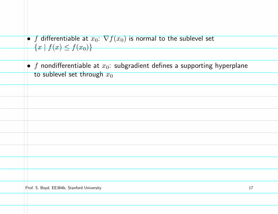
• f differentiable at x0: ∇f(x0) is normal to the sublevel set{x | f(x) ≤ f(x0)}

• f nondifferentiable at x0: subgradient defines a supporting hyperplaneto sublevel set through x0


The conjugate function

the conjugate of a function f is

f∗(y) = supx∈dom f

(yTx − f(x))

f(x)

(0,−f∗(y))

xy

x

• f∗ is convex (even if f is not)

• will be useful in chapter 5


examples

• negative logarithm f(x) = − log x

f∗(y) = supx>0

(xy + log x)

=

{

−1 − log(−y) y < 0∞ otherwise

• strictly convex quadratic f(x) = (1/2)xTQx with Q ∈ Sn++

f∗(y) = supx

(yTx − (1/2)xTQx)

=1

2yTQ−1y


Quasiconvex functions

f : Rn → R is quasiconvex if dom f is convex and the sublevel sets

Sα = {x ∈ dom f | f(x) ≤ α}

are convex for all α

α

β

a b c

• f is quasiconcave if −f is quasiconvex

• f is quasilinear if it is quasiconvex and quasiconcave


Examples

•√

|x| is quasiconvex on R

• ceil(x) = inf{z ∈ Z | z ≥ x} is quasilinear

• log x is quasilinear on R++

• f(x1, x2) = x1x2 is quasiconcave on R2++

• linear-fractional function

f(x) =aTx + b

cTx + d, dom f = {x | cTx + d > 0}

is quasilinear

• distance ratio

f(x) =‖x − a‖2

‖x − b‖2, dom f = {x | ‖x − a‖2 ≤ ‖x − b‖2}

is quasiconvex


internal rate of return

• cash flow x = (x0, . . . , xn); xi is payment in period i (to us if xi > 0)

• we assume x0 < 0 and x0 + x1 + · · · + xn > 0

• present value of cash flow x, for interest rate r:

PV(x, r) =

n∑

i=0

(1 + r)−ixi

• internal rate of return is smallest interest rate for which PV(x, r) = 0:

IRR(x) = inf{r ≥ 0 | PV(x, r) = 0}

IRR is quasiconcave: superlevel set is intersection of halfspaces

IRR(x) ≥ R ⇐⇒n

∑

i=0

(1 + r)−ixi ≥ 0 for 0 ≤ r ≤ R


Properties

modified Jensen inequality: for quasiconvex f

0 ≤ θ ≤ 1 =⇒ f(θx + (1 − θ)y) ≤ max{f(x), f(y)}

first-order condition: differentiable f with cvx domain is quasiconvex iff

f(y) ≤ f(x) =⇒ ∇f(x)T (y − x) ≤ 0

x∇f(x)

sums of quasiconvex functions are not necessarily quasiconvex


Log-concave and log-convex functions

a positive function f is log-concave if log f is concave:

f(θx + (1 − θ)y) ≥ f(x)θf(y)1−θ for 0 ≤ θ ≤ 1

f is log-convex if log f is convex

• powers: xa on R++ is log-convex for a ≤ 0, log-concave for a ≥ 0

• many common probability densities are log-concave, e.g., normal:

f(x) =1

√

(2π)n det Σe−

12(x−x̄)TΣ−1(x−x̄)

• cumulative Gaussian distribution function Φ is log-concave

Φ(x) =1√2π

∫ x

−∞

e−u2/2 du


Properties of log-concave functions

• twice differentiable f with convex domain is log-concave if and only if

f(x)∇2f(x) � ∇f(x)∇f(x)T

for all x ∈ dom f

• product of log-concave functions is log-concave

• sum of log-concave functions is not always log-concave

• integration: if f : Rn × Rm → R is log-concave, then

g(x) =

∫

f(x, y) dy

is log-concave (not easy to show)


consequences of integration property

• convolution f ∗ g of log-concave functions f , g is log-concave

(f ∗ g)(x) =

∫

f(x − y)g(y)dy

• if C ⊆ Rn convex and y is a random variable with log-concave pdf then

f(x) = prob(x + y ∈ C)

is log-concave

proof: write f(x) as integral of product of log-concave functions

f(x) =

∫

g(x + y)p(y) dy, g(u) =

{

1 u ∈ C0 u 6∈ C,

p is pdf of y


example: yield function

Y (x) = prob(x + w ∈ S)

• x ∈ Rn: nominal parameter values for product

• w ∈ Rn: random variations of parameters in manufactured product

• S: set of acceptable values

if S is convex and w has a log-concave pdf, then

• Y is log-concave

• yield regions {x | Y (x) ≥ α} are convex


Convexity with respect to generalized inequalities

f : Rn → Rm is K-convex if dom f is convex and

f(θx + (1 − θ)y) �K θf(x) + (1 − θ)f(y)

for x, y ∈ dom f , 0 ≤ θ ≤ 1

example f : Sm → Sm, f(X) = X2 is Sm+ -convex

proof: for fixed z ∈ Rm, zTX2z = ‖Xz‖22 is convex in X, i.e.,

zT (θX + (1 − θ)Y )2z ≤ θzTX2z + (1 − θ)zTY 2z

for X,Y ∈ Sm, 0 ≤ θ ≤ 1

therefore (θX + (1 − θ)Y )2 � θX2 + (1 − θ)Y 2


Documents

P A G E S 2 1 6 T O 2 3 1 O F h ttp ://w w w .c se .iitb ...cs709/notes/enotes/basicsOfUnivariate... · ... in te rsp e rse d w ith p a g e s b e tw e e n 2 3 9 a n d 2 5 3 a n d