Embed Size (px)
Citation preview

Overview of slides 04
1 Stochastic processes, in particular Markov processesStochastic processesStochastic matrix / transition matrix
2 Markov chain Monte CarloMetropolis algorithmAutocorrelationsAlternatives to Metropolis
3 Ising modelOverviewPhase transition & critical phenomenaSimulation
4 Summary
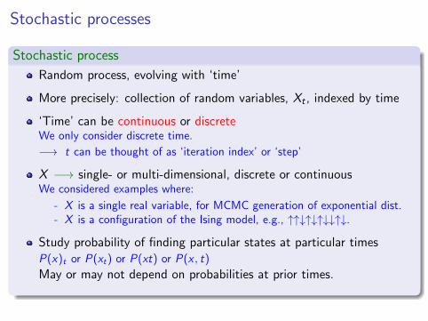
Stochastic processes
Stochastic process
Random process, evolving with ‘time’
More precisely: collection of random variables, Xt , indexed by time
‘Time’ can be continuous or discreteWe only consider discrete time.
−→ t can be thought of as ‘iteration index’ or ‘step’
X −→ single- or multi-dimensional, discrete or continuousWe considered examples where:
- X is a single real variable, for MCMC generation of exponential dist.- X is a configuration of the Ising model, e.g., ↑↑↓↑↓↑↓↓↑↓.
Study probability of finding particular states at particular timesP(x)t or P(xt) or P(xt) or P(x , t)
May or may not depend on probabilities at prior times.

Stochastic processes
Independent random process
Simplest case. Future probability independent of present or past:
P(xntn|xn−1tn−1 . . . x1t1) = P(xntn)
Completely memory-less. Special case of Markov process.
Markov process
Future probability depends only on present, independent of past:
P(xntn|xn−1tn−1 . . . x1t1) = P(xntn|xn−1tn−1)
Limited memory — Only most recent value counts

Markov processes
Transition probabilities
A Markov chain is described by transition probabilities
T (X → Y ) or TX→Y
When states space is finite:Can represent as matrix with elements Tij = T (Xi → Xj)
−→ stochastic matrix or transition matrix or Markov matrix

Markov processes: transition graph + transition matrix
102 3 Markov Chain Monte Carlo
be reached from x in one iteration is the neighborhood of x, denotedby Nx. Each such directed edge has a probability pxy associated withit. This is the probability that the edge will be chosen on the nextiteration when the chain currently is in the state x.
x1
x2
x3
x4
p12
p21
p23
p31
p43
p14
p11
p44 p34
Fig. 3.1. The graph representation of a four-state Markov chain. Its corre-sponding transition matrix is
p11 p12 0 p14
p21 0 p23 0p31 0 0 p34
0 0 p43 p44
.
The chain starts in some state, say X0, which may be chosen ran-domly according to a starting distribution or just assigned. From thenon, the chain moves from state to state on each iteration according tothe neighborhood transition probabilities. Given that the chain is instate x on some iteration, the next state is chosen according to thediscrete density given by pxy : y ∈ Nx. Notice that the sum of theoutgoing probabilities from each vertex x must be 1 to cover all thepossible transitions from x,
∑
y∈Nx
pxy = 1, for all x ∈ Ω. (3.1)
The selection is implemented using any of the roulette wheel selectionmethods. In the graph, the chain moves along the chosen edge to the
Sh
on
kw
iler
&M
end
ivil:
Exp
lorations
inMonte
Carlo
Methods

Transition matrix / stochastic matrix
Row stochastic matrix
Matrix with elements Tij = T (Xi → Xj).
Sum of each row = 1 (system must end up in some state)
Has one eigenvalue exactly =1. All other eigenvalue magnitudes < 1.→ follows from Perron-Frobenius theorem.
If probabilities of states atstep n is row vector pn, then
pn+1 = pnT
The left eigenvectorcorresponding to eigenvalue 1 isthe stationary state
Analogy: power method
Column stochastic matrix: elements Tij = T (Xj → Xi)
Right eigenvectors, column vectors for probabilityRow stochastic matrix is more commonly used. :-(

Markov process: Master Equation and Detailed Balance
Master equation
P(X , tn+1)− P(X , tn) =∑Y
[P(Y , tn)TY→X − P(X , tn)TX→Y
]
Derived using:
P(X , tn+1) =
∑Y
P(Y , tn)TY→X
P(X , tn) = P(X , tn)∑Y
TX→Y
Detailed balance — condition for stationary distribution
P(X )T (X → Y ) = P(Y )T (Y → X )
Sufficient, not necessary
Markov chain Monte Carlo
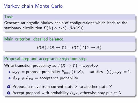
Task
Generate an ergodic Markov chain of configurations which leads to thestationary distribution P(X ) ∝ exp(−βH(X ))
Main criterion: detailed balance
P(X )T (X → Y ) = P(Y )T (Y → X )
Proposal step and acceptance/rejection step
Write transition probability as T (X → Y ) = ωXYAXY
ωXY = proposal probability Pprop.(Y |X ), satisfies∑
Y ωXY = 1.
AXY 6= AYX = acceptance probability
1 Propose a move from current state X to another state Y
2 Accept proposal with probability AXY , otherwise stay put at X

Metropolis algorithm
Metropolis
Ensure symmetric proposal probability: ωXY = ωYX
Use acceptance probability
AXY = min
(1,
P(Y )
P(X )
)=
1 P(X ) ≤ P(Y )P(Y )P(X ) P(X ) > P(Y )
Metropolis-Hastings
More general: proposal probability need not be symmetric.Use acceptance probability
AXY = min
(1,
P(Y )ωXY
P(X )ωYX
)

Metropolis algorithm
Metropolis
Use symmetric proposal probability: ωXY = ωYX . Acceptance probability
AXY = min
(1,
P(Y )
P(X )
)=
1 P(X ) ≤ P(Y )P(Y )P(X ) P(X ) > P(Y )
Proof of detailed balance
T (X → Y )
T (Y → X )=ωXYAXY
ωYXAYX=
AXY
AYX
If P(X ) ≤ P(Y ) then AXY = 1, AYX = P(X )/P(Y )If P(X ) > P(Y ) then AXY = P(Y )/P(X ), AYX = 1In either case
T (X → Y )
T (Y → X )=
AXY
AYX=
P(Y )
P(X )=⇒ detailed balance

Metropolis algorithm
Ergodicity
Depends on ωXY
It must be possible to reach any Y from any X after a series of steps.
Statistical physics
P(X ) ∝ e−βH(X ) =⇒ P(Y )
P(X )= e−β∆H
Don’t need to know normalization factor Z =∑
X e−βH(X )
→ partition function, might be impossible to calculate
Metropolis acceptance probabilities for Statistical physics
AXY =
1 if H(Y ) ≤ H(X )
e−β∆H if H(Y ) > H(X )

Autocorrelations
Two successive configurations in Markov chain are “close” in phase space=⇒ any quantity will have similar values on the two configs
If φ is some scalar property, nearby values of φ are correlated.
〈Φ[Xn]Φ[Xn+1]〉 6= 〈Φ[Xn]〉〈Φ[Xn+1]〉 i.e., 6= 〈Φ〉2
Define autocorrelation function:
R(t) = 〈Φ[Xn]Φ[Xn+t ]〉 − 〈Φ[Xn]〉〈Φ[Xn+t ]〉
Nonzero for small t, should vanish for large t.
We want Monte Carlo samples to be statistically independent
Save Φ values spaced from each other along Markov chain.

Autocorrelations
Autocorrelation time τ
R(t) = 〈Φ[Xn]Φ[Xn+t ]〉 − 〈Φ〉2 ∼ Ce−t/τ
τ measures “memory” of the Markov process
Configurations separated by t & 2τ are ≈ statistically independent
How to make τ small? → improved update/proposal schemesE.g., cluster updates
Autocorrelations increase dramatically near phase transitions→ critical slowing down
Statistical uncertainties are underestimated if autocorrelations areignored

Alternatives to Metropolis
Reminder: Metropolis acceptance probabilities
AXY =
1 if H(Y ) ≤ H(X )
e−β∆H if H(Y ) > H(X )
Detailed balance can be satisfied by other acceptance probabilities.
1 Glauber algorithm:
AXY =1
1 + eβ∆H
2 Heat-bath algorithm

Ising model
Simple model of (anti)ferromagnetism
We have a lattice of spins σi = ±1
H = −J∑<ij>
σiσj − B∑i
σi ;∑<ij>
= sum over nearest neighbours
J > 0: energy minimized by aligning spins → ferromagnet
J < 0: energy minimized by anti-aligning neighboring spins →antiferromagnet
Magnetic field B > 0: tries to have spins all +1.
Physics depends on lattice: square, cube, triangular, honeycomb,Kagome, pyrochlore,...

Ising model
Simple model of (anti)ferromagnetism
We have a lattice of spins σi = ±1
H = −J∑<ij>
σiσj − B∑i
σi ;∑<ij>
= sum over nearest neighbours
1D Ising chain: analytically solvable. No phase transitions.
2D Ising on square lattice: B = 0:“Solvable”, difficult → Onsager solution.Has a phase transition at T = Tc ≈ 2.2692J
No analytical solution is known for d = 3, for B 6= 0, other lattices.Many types of interesting physics in different latticesEven more types of interesting physics in models with continuousdegrees of freedom, e.g., Heisenberg models.→ Monte Carlo simulations are essential

Phase transition of Ising modelFocus on 2D square lattice, B = 0.
Phase transition
There is a second order phase transition at temperature Tc
Magnetization per site:
µ =M
num.sites=
∑i σi
num.sites
Spontaneous magnetization at low T :
T > Tc : µ = 0
T < Tc : µ 6= 0

Phase transition of 2D Ising model
Second-order Phase transition
2nd-order → µ vanishes continuously
Critical behaviour: with t ≡ (Tc − T )/Tc ,
µ ∼ tβ , χ ∼ t−γ , Cv ∼ (−t)−α
The critical exponents α, β, γ, . . . are universal:Same behaviour for all systems with the same symmetries and dimensions
χ → susceptibility,∂M
∂B
∣∣∣∣B=0
Cv → spec. heat,∂H
∂T

Phase transition of 2D Ising model
Second-order Phase transition
Critical behaviour: with t ≡ (Tc − T )/Tc ,
µ ∼ tβ , χ ∼ t−γ , Cv ∼ (−t)−α
2D Ising universality class:
γ = 7/4Susceptibility diverges at criticalpoint!
α = 0, but specific heat alsodiverges → logarithmic divergence.
finite-size
Actual divergence only seen in infinite-size system.

Simulation of Ising model
Metropolis algorithm
1 Start with all σi = 1 (cold start) or random ±1 (hot start)
2 Sweep through all sites of lattice successively.(Or pick a site at random at each step.)For each site:
I Calculate the energy difference ∆E if you flip that spin σi → −σiI If ∆E < 0 flip the spinI otherwise generate a uniform random r ∈ (0, 1),
flip the spin if r < e−β∆E
3 Compute + save physical quantities (µ,E etc)maybe only every m-th step to minimize correlations
4 Repeat for N sweeps

Simulation results
T ≈ 0.9Tc

Simulation results
T ≈ Tc
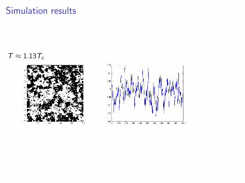
Simulation results
T ≈ 1.13Tc

Simulation results
T ≈ 1.6Tc

Finite volume issues
Boundary conditions
We want to study a macroscopic (nearly infinite) system
the finite system we simulate is only a subsample of this
use periodic boundary conditions to mimic surroundings
No phase transitions on a finite volume
All thermodynamic functions on finite V are smooth functions of T .
Not insurmountable: use finite volume scaling
As V grows the crossover becomes sharper
Extrapolate to 1/V = 0
There are critical exponents for finite volume scaling

Summary
Markov processes
A Markov process is a stochastic process with no memory
Described by transition probabilities
All Markov processes obey the master equation
Detailed balance is a sufficient condition for a stationary process
Markov chain Monte Carlo
Use an ergodic Markov chain to create a statistical distribution ofconfigurations
Metropolis: all-purpose algorithm for Monte Carlo simulations
Application to statistical physics (condensed matter) systemseg Ising model
Autocorrelations need to be monitored