Sandia National Laboratories is a multimissionlaboratory managed and operated by National Technology & Engineering Solutions of Sandia, LLC, a wholly owned subsidiary of Honeywell International Inc., for the U.S. Department of

Energy’s National Nuclear Security Administration under contract DE-NA0003525.

Overview of Molecular Dynamics

Stan Moore

Vir tual LAMMPS Workshop and Symposium 2021

SAND2021-9693 C

Molecular Dynamics: What is it?

Mathematical Formulation

Classical MechanicsAtoms are Point Masses: r1, r2, ..... rNPositions, Velocities, Forces: ri, vi, FiPotential Energy Function = V(rN)

6N coupled ODEs

Interatomic Potential

Initial Positions and Velocities

Positions and Velocities at many later times

dridt

= vi

dvidt

=Fimi

Fi = −ddri

V rN( )

What is MD good for?

Quantum mechanical electronic structure calculations (QM) provide accurate description of mechanical and chemical changes on the atom-scale: 10x10x10~1000 atoms

Atom-scale phenomena drive a lot of interesting physics, chemistry, materials science, mechanics, biology…but it usually plays out on a much larger scale

Mesoscale: much bigger than an atom, much smaller than a glass of soda.

QM and continuum/mesoscale models (CM) can not be directly compared.

Distance

Tim

e

Å mm

10-1

5 s

10-6

s

QM

ContinuumMesoscale

ModelsLarge-Scale MD simulation

CTH images courtesy of David Damm, Sandia

CM/CTH

MD/LAMMPS

n Small molecular dynamics (MD) simulations can be directly compared to QM results, and made to reproduce them

n MD can also be scaled up to millions (billions) of atoms, overlapping the low-end of CM

n Limitations of MD orthogonal to CMn Enables us to inform CM models with quantum-

accurate results Picture of soda glass: by Simon Cousins from High Wycombe, England - Bubbles, CC BY 2.0, https://commons.wikimedia.org/w/index.php?curid=23020999

MD Versatility

Chemistry

Materials Science

Biophysics

Granular Flow

Coupling to Solid

Mechanics

Atoms can be modeled as points (most common), finite-size spheres, or other shapes (e.g. ellipsoids)Can model atomic-scale (all-atom model) or meso/continuum scale with MD-like modelsTypically use an orthogonal or triclinic (skewed) simulation cellCommonly use periodic boundary conditions: reduces finite size effects from boundaries and simulates bulk conditions

MD Basics 2D Triclinic

MD Time Integration Algorithm

6

• Most codes and applications use variations and extensions to the Størmer-Verlet explicit integrator:

• Only second-order : δE = |<E>-E0| ~ Δt2, but….

• time-reversible map: switching sign of Δt takes you back to initial state

• measure-preserving: Volume of differential cube (δv,δx) is conserved (but not shape).

• symplectic: Conserves sum of areas of differential parallelogram (δv,δx) projected onto each particular (vi,xi) plane

For istep < nsteps :

v← v+ Δt2F

x← x+Δt vCompute F x( )

v← v+ Δt2F

Velocity form of Størmer-Verlet

−1 0 1 2 3 4 5 6 7 8 9

−2

−1

1

2

A

ϕπ/2(A)ϕπ(A)

B

ϕπ/2(B)

ϕπ(B)ϕ3π/2(B)

Figure 3: Area preservation of the flow of Hamiltonian systems

Figure 3 shows level curves of this function, and it also illustrates the area preser-vation of the flow ϕt. Indeed, by Theorem 2, the areas of A and ϕt(A) as wellas those of B and ϕt(B) are the same, although their appearance is completelydifferent.

We next show that symplecticity of the flow is a characteristic property forHamiltonian systems. We call a differential equation y = f(y) locally Hamilto-nian, if for every y0 ∈ U there exists a neighbourhood where f(y) = J−1∇H(y)for some functionH .

Theorem 3 Let f : U → R2d be continuously differentiable. Then, y = f(y) islocally Hamiltonian if and only if its flow ϕt(y) is symplectic for all y ∈ U andfor all sufficiently small t.

Proof. The necessity follows from Theorem 2. We therefore assume that the flowϕt is symplectic, and we have to prove the local existence of a functionH(y) suchthat f(y) = J−1∇H(y). Differentiating (17) and using the fact that ∂ϕt/∂y0 is asolution of the variational equation Ψ = f ′

(ϕt(y0)

)Ψ, we obtain

d

dt

((∂ϕt

∂y0

)TJ

(∂ϕt

∂y0

))=

(∂ϕt

∂y0

)(f ′

(ϕt(y0)

)TJ + Jf ′

(ϕt(y0)

))(∂ϕt

∂y0

)= 0.

Putting t = 0, it follows from J = −JT that Jf ′(y0) is a symmetric matrix forall y0. The Integrability Lemma below shows that Jf(y) can be written as thegradient of a functionH(y).

8

Ernst Hairer, Lubich, Wanner, Geometric Numerical Integration (2006)

MD Time Integration Algorithm

7

• time-reversibility and symplecticity: global stability of Verlet trumps local accuracy of high-order schemes

• More specifically, it can be shown that for Hamiltonian equations of motion, Størmer-Verletexactly conserves a “shadow” Hamiltonian and E-ES ~ O(Δt2)

• For users: no energy drift over millions of timesteps• For developers: easy to decouple integration scheme from efficient algorithms for force evaluation,

parallelization.• Symplectic high-order Runge-Kutta methods exist, but not widely adopted for MD

32 atom LJ cluster, 200 million MD steps, Δt=0.005, T=0.4

0 50 100 150 200MD Timesteps [Millions]

0

5

ΔE

[10-4ε] -0.1

0.1

Statistical Mechanics: relates macroscopic observations (such as temperature and pressure) to microscopic states (i.e. atoms)

Phase space: a space in which all possible states of a system are represented. For Nparticles: 6N-dimensional phase space (3 position variables and 3 momentum variables for each particle)

Ensemble: an idealization consisting of a large number of virtual copies of a system, considered all at once, each of which represents a possible state that the real system might be in, i.e. a probability distribution for the state of the system

Statistical Mechanics Basics

Using the velocity-verlet time integrator gives the microcanonical ensemble (NVE). How to simulate canonical (NVT) or isothermal-isobaric (NPT) ensembles?

Temperature is related to atom velocities through statistical mechanics, pressure is related to volume of the simulation cell

Could just scale velocities and volume to the exact desired values, but this does not allow for fluctuations with a distribution typical for the ensemble

Instead Nose-Hoover style integrators are commonly used: dynamic variables are coupled to the particle velocities (thermostatting) and simulation box dimensions (barostatting)

Nose-Hoover uses a damping parameter specified in time units which determines how rapidly the temperature or pressure is relaxed. If the damping parameter is too small, the temperature/pressure can fluctuate wildly; if it is too large, the temperature/pressure will take too long to equilibrate

Thermostats and Barostats

Quantum chemistry: solves Schrödinger equation to get forces on atoms. Accurate but very computationally expensive and only feasible for small systems

Molecular dynamics: uses empirical force fields, sometimes fit to quantum data. Not as accurate but much faster.

Typically only interact with atoms in a spherical cutoff and only consider pair-wise or three-body interactions

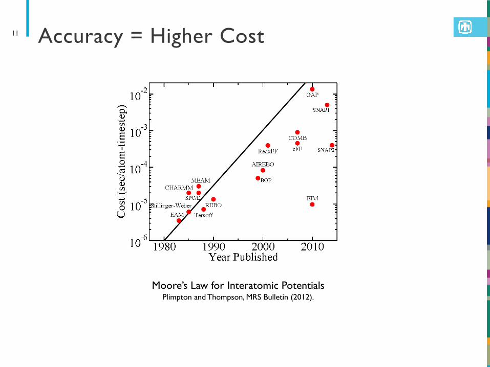
Interatomic Potentials

attractive tail

repulsive wall

Lennard-Jones Potential

Pair-wise distance

Inte

ract

ion

Ener

gy

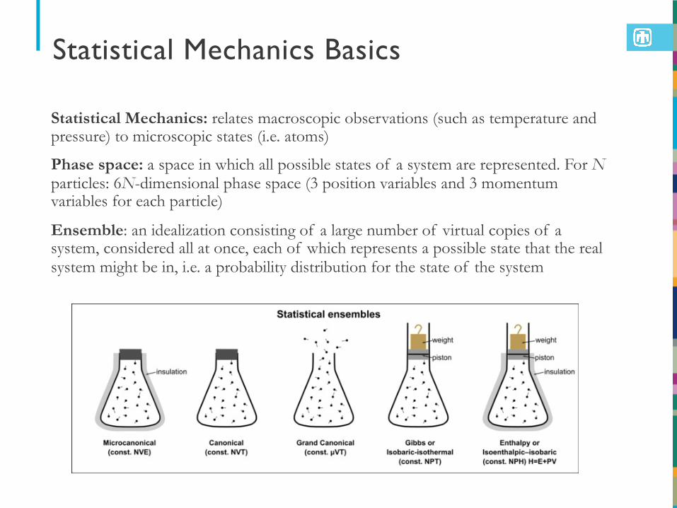
Accuracy = Higher Cost11

Moore’s Law for Interatomic PotentialsPlimpton and Thompson, MRS Bulletin (2012).

Neighbor ListsNeighbor lists are a list of neighboring atoms within the interaction cutoff + skin for each central atom

Extra skin allows lists to be built less often

12

cutoff

Basic MD Timestep

During each timestep (without neighborlist build):

1. initial integrate2. compute forces (pair, bonds, etc.)3. final integrate4. output (if requested on this timestep)

*Computation of diagnostics (i.e. thermodynamic properties) can be scattered throughout the timestepMay also occasionally build neighborlist for diagnostics

13

Long-Range Electrostatics (Optional)

Truncation doesn’t work well for charged systems due to long-ranged nature of Coulombic interactions

Use reciprocal-space method to add long-range electrostatics:◦ Ewald Sum—uses discrete Fourier transform, potentially most accurate, but slow

for large systems◦ Particle-particle particle-mesh (PPPM) and Smooth particle-mesh Ewald

(SPME)—interpolates atom charges to grid and uses fast Fourier Transforms (FFTs), usually fastest

Other real-space methods sometimes used: fast multipole, multilevel summation

14

Domain decomposition: each processor owns a portion of the simulation domain and atoms therein

MPI Parallelization Approach15

proc 1 proc 2

proc 3 proc 4

*This method is used by many MD codes (including LAMMPS) use, but there are other strategies as well

The processor domain is also extended include needed ghost atoms (copies of atoms located on other processors)

Ghost Atoms16

proc 1

local atoms

ghost atoms

Basic MD Timestep

During each timestep (without neighborlist build):

1. initial integrate2. compute forces (pair, bonds, etc.)3. final integrate4. output (if requested on this timestep)

*Computation of diagnostics (i.e. thermodynamic properties) can be scattered throughout the timestepMay also occasionally build neighborlist for diagnostics

17

Basic MD Timestep with MPI comm

During each timestep (without neighborlist build):

1. initial integrate2. MPI communication: send atom coordinates to ghost atoms3. compute forces (pair, bonds, etc.)4. MPI communication: sum atom forces from ghost atoms (if newton flag on)5. final integrate6. output (if requested on this timestep)

*Computation of diagnostics (fixes or computes) can be scattered throughout the timestep

18

Parallel MD Performance

Strong scaling: hold system size fixed while increasing processor count (# of atoms/processor decreases)

Weak scaling: increase system size in proportion to increasing processor count (# of atoms/processor remains constant)

For perfect strong scaling, doubling the processor count cuts the simulation time in half

For perfect weak scaling, the simulation time stays exactly the same when doubling the processor count

Harder to maintain parallel efficiency with strong scaling because the compute time decreases relative to the communication time

High communication overhead when strong scaling to a few 100 atoms/proc (depends on cost of the force-field)

MD parallelizes well: major parts of timestep (forces, neighbor list build, time integration) can be done in parallel through domain decomposition

19

MD Codes

There are several freely-available parallel molecular dynamics codes:

CHARMM, AMBER, GROMACS, NAMD, and Tinker are designed primarily for modeling biological systems. AMBER and CHARMM are the original classic codes in this genre. Gromacs, NAMD, and Tinker are more recently developed codes.

DL_POLY includes potentials for a variety of biological and non-biological materials. LAMMPS is focused on materials but versatile. HOOMD is a very fast materials MD code designed to run on GPUs.

NWChem is both a molecular dynamics and quantum code which can model a variety of materials.

We will now learn about LAMMPS in this tutorial.

20