HAL Id: hal-02085660https://hal.archives-ouvertes.fr/hal-02085660

Submitted on 30 Mar 2019

HAL is a multi-disciplinary open accessarchive for the deposit and dissemination of sci-entific research documents, whether they are pub-lished or not. The documents may come fromteaching and research institutions in France orabroad, or from public or private research centers.

L’archive ouverte pluridisciplinaire HAL, estdestinée au dépôt et à la diffusion de documentsscientifiques de niveau recherche, publiés ou non,émanant des établissements d’enseignement et derecherche français ou étrangers, des laboratoirespublics ou privés.

Overhead lines Dynamic Line rating based onprobabilistic day-ahead forecasting and risk assessment

Romain Dupin, George Kariniotakis, Andrea Michiorri

To cite this version:Romain Dupin, George Kariniotakis, Andrea Michiorri. Overhead lines Dynamic Line rating basedon probabilistic day-ahead forecasting and risk assessment. International Journal of Electrical Powerand Energy Systems, Elsevier, 2019, 110, pp.565-578. �10.1016/j.ijepes.2019.03.043�. �hal-02085660�

1

ATTENTION, this is a preprint of:

Romain Dupin, George Kariniotakis, Andrea Michiorri, “Overhead lines Dynamic Line rating based on probabilistic day-ahead forecasting and risk assessment” , International Journal of Electrical Power & Energy Systems, Volume 110, 2019, Pages 565-578, ISSN 0142-0615, https://doi.org/10.1016/j.i jepes.2019.03.043

Available at : http://www.sciencedirect.com/science/article/pii/S014206151831891X

© 2019. This manuscript version is made available under the CC -BY-NC-ND 4.0 l icense http://creativecommons.org/licenses/by -nc-nd/4.0/

Overhead lines Dynamic Line Rating based on Probabilistic Day-Ahead Forecasting and Risk

Assessment

Romain Dupin, George Kariniotakis, Andrea Michiorri

MINES ParisTech, PSL University,

Centre for Processes, Renewable Energies and Energy Systems (PERSEE),

1 Rue Claude Daunesse, CS 10207, 06904 Sophia Antipolis Cedex, France.

Contact: andrea.michiorri@mines-paristech.fr

Abstract: Dynamic Line Rating is a technology devised to modify an overhead line’s current-carrying capacity based on weather observation. The benefits of this modification may include reduced congestion costs, an increased renewable energy penetration rate, and improved network reliability. DLR is already well developed, but few papers in the literature investigate DLR day-ahead forecasting. The latter is central to DLR development since many of the decisions related to grid management are taken at least on a day-ahead basis. In this paper, two problems related to DLR forecasts are dealt with: how to achieve precise, reliable calculations of day-ahead forecasts of overhead line ampacity and how to define a methodology to calculate safe rating values using these forecasts. On the first point, four machine-learning algorithms were evaluated, identifying the best approach for this problem and quantifying the potential performance. On the second point, the developed methodology was tested and compared to the current static line rating approach.

Keywords: Dynamic Line Rating, Numerical Weather Predictions, probabilistic forecasts, smart grid.

NOMENCLATURE

ACSR Aluminium Conductor Steel reinforced

AR Accepted Risk (strategy)

CRPS Continuous Ranked Probability Score

DLR Dynamic Line Rating

ECMWF European Centre for Middle range Weather Forecast

2

FQ Fixed Quantile (strategy)

KDE Kernel Density Estimator

MAPE Mean Absolute Percentage Error

MDNN Mixture Density Neural Network

NWP Numerical Weather Prediction

PCA Principal Component Analysis

PDF Probability Density Function

QLR Quantile Linear Regression Model

QRF Quantile Regression Forest

QS Quantile Scores

RES Renewable Energy Source

RTLR Real Time Thermal Rating

SLR Static Line Rating

Weights associated with the Gaussian PDFs for the MDNN

βc [K-1] Conductor’s thermal expansion factor

Mean values of the Gaussian PDFs for the MDNN

Standard deviations of the Gaussian PDFs for the MDNN

Kernel function used in the KDE model

[K] Ambient temperature

[K] Conductor’s temperature

Generic input for the forecast known at time t

, Generic forecast calculated at time t for time t+h

[W/mK] Convective cooling factor

[W/mK] Radiative heat exchange constant

[W/mK] solar gain constant

Ac [m2] Conductor’s cross-sectional area

C1 *€+ Cost associated with not supplying the load

C2 *€+ Cost associated with damages to objects and people

C3 *€+ Cost associated with the conductor’s ageing

Di *€+ Damage associated with event i

Ec [Pa] Conductor’s Young modulus

EV *€+ Expected Value

Fp [N] Conductor’s linear weight

Ft [N] Conductor’s tensile strength

h [s] Horizon of the forecast

Iq [A] RTLR relative to probability q

3

l [m] Length of the whole circuit

Lsag [m] Conductor’s sag

Lspan [m] Conductor’s span length

Pi Probability of the event i

R [/m] Conductor resistance per unit length

RK *€+ Risk

Sr [W/m2] Solar radiation

t [s] Time of forecast calculation

V [V] Voltage level of the line

Wd [°] Wind direction

Ws [m/s] Wind speed

1 INTRODUCTION

Currently, power system operators are facing several challenges, due to an increase in electrical consumption and peak demand, the deregulation of electricity markets and the increasing penetration of Renewable Energy Sources (RES) [1]. Due to these latter factors, grid sections are often operated closer to their regulatory limits in terms of stability, voltage limits or ampacity. From a network operator point of view, network reinforcement is often the default option for alleviating these problems. However, this is a very capital-intensive option, and building permits are difficult to obtain due to increasing environmental concerns. It is in this context that the Dynamic Line Rating (DLR) is being investigated.

To define DLR, it is necessary to understand why a current limit is designed for overhead electrical lines. In order to maintain a minimum clearance distance between overhead electric lines and items located under the lines, the line’s core temperature must remain lower than a defined value. Due to the influence of the Joules effect on that temperature, a maximum current must be defined in order to respect this constraint. Traditionally, this limit is set as static, and fixed for a given period, such as a season: this is known as Static Line Rating (SLR). The limit can also be set using DLR, in which case, unlike SLR, it is dynamically modified at each time step in accordance with the weather characteristics and so the instantaneous value of the line rating, the Real-Time Line Rating (RTLR). Note that most studies do not differentiate between RTLR and DLR, for this reason, it will be stressed here and elsewhere the nature and importance of this difference in order to facilitate the understanding of this paper. RTLR is the actual value of the ampacity of the circuit, it is an implicit value, and it cannot be measured but only calculated in real time or after the event. DLR is the value of rating that the network operator (DSO or TSO) decides to apply to the circuit before the event. Central to this paper is the idea of setting the DLR from forecasts of the RTLR.

Here, it is given a simple example to illustrate the difference between RTLR, DLR and SLR. Considering the steady state thermal model described in [2], [3], conductor’s properties and the suggested conservative values for weather parameters (e.g. wind speed at 0.5 m/s, wind direction perpendicular to the cable, null solar radiation and air temperature at 20°C), a static limit for the ampacity (the SLR) is defined for a given period such as a season as described in [4]. For the same line, it is possible to calculate the actual real-time ampacity limit (the RTLR) by considering the real values of the weather parameters. The line operator needs to fix in advance a limit for the ampacity of the line, for example in order to set protections. This can be the SLR or, in case of dynamic ratings, the DLR.

4

Fig. 1 shows the resulting comparison between SLR and RTLR for the same line for one week. We can observe a large variation in RTLR and the potential unlocked capacity.

Fig. 1. Evolution of Static Line Rating and Real Line Rating over a 3-day period

Currently, devices are increasingly used to estimate RTLR. For example, several devices to monitor conductor ampacity have been developed [5], [6], along with systems to estimate RTLR over large network areas using weather data. In order to fully exploit the advantages provided by DLR, circuit ampacity forecasts are often required, as most grid operation decisions are taken at least one day ahead. However, day-ahead RTLR forecasting has not been explored deeply and little information is available in the literature.

The potential benefits of considering DLR instead of SLR for network operations are multiple and have already been studied in the literature. For example, [7] shows how DLR can help increase RES penetration without grid reinforcement, while [8] demonstrates how grid reliability can be improved and [9] proposes a review of relevant studies.

Some studies also show the potential impact of DLR on economic dispatch. However, due to the fact that this is not a real-time functionality, [10] shows the need for developing RTLR forecasts for this application. In a similar way, [11] considers RTLR forecasts in his study of DLR on the total trading capacity between two countries, given that most exchange operations are decided at least 24 hours in advance. In the case where line constraints limit the trading capacity in electricity markets, the use of RTLR forecasts could contribute to considerable financial savings.

The aim of the present paper is to develop a probabilistic approach for day-ahead RTLR forecasting

based on machine learning methods and using weather station measurements and numerical weather

predictions as input. Different models are compared using both deterministic and probabilistic evaluation

criteria. Data are considered from a real-world case in Northern Ireland, UK. The forecasts provided are

assessed for their ability to increase the rating while maintaining significant safety margins. Furthermore,

the paper presents two possible strategies for setting DLR based on probabilistic forecasts and compares

their behaviour in terms of increased ampacity and line operating risk. The paper ends with a discussion

of the potential improvements and use of probabilistic RTLR forecasts.

The key contributions of this paper can be summarized as follows: 1) identification of the most efficient

model for probabilistic RTLR forecasting through the comparison of several advanced models, 2)

evaluation of the performance of RTLR probabilistic forecasting according to relevant metrics, and 3)

definition of methodologies for the definition of day-ahead DLR from probabilistic RTLR forecasts.

0

500

1000

1500

2000

2500

0 3 6 9 12 15 18 21 24 27 30 33 36 39 42 45 48 51 54 57 60 63 66 69

Am

pac

ity

[A]

Time [hh]

SLR RTLR DLR

5

2 DLR FORECASTING STATE OF THE ART OVERVIEW

The literature on DLR and RTLR forecasting is limited compared to that on forecasting other quantities

central to power system management, like electricity demand and renewable generation. The existing

methods for RTLR forecasting can be categorized into two groups, depending on the forecast time horizon:

- For short-term horizons of 0-6 hours ahead, time-series approaches are commonly used to forecast

weather variables and ampacity using historic observations as input i.e. [12]–[15].

- For longer-term horizons of 6-48 hours ahead, statistical approaches are mainly used considering

Numerical Weather Predictions (NWP) as input.

Since the subject of this paper is day-ahead forecasts, the following literature review focuses on methods

proposed for this time frame. Several methods exist today. A state of the art including research projects

that develop research on RTLR forecasting is presented in [16]. In the context of the European project

TWENTIES [17], an RTLR forecast algorithm has been developed, using multi-linear regression, with

horizons varying from 24 hours to 48 hours ahead. The input is historical data collected on two Belgian

150 kV overhead lines, for a limited period of about three months, together with high-resolution NWPs.

For safety reasons, the probability that DLR forecasts will be higher than future observations has been set

at 2%. It was shown that the forecasted DLR was on average 10% higher than the SLR.

In [18], the authors used NWPs from the National Oceanic Atmospheric Administration models and,

with the provided mean and standard deviation values, defined a PDF for each weather parameter. They

then ran a Monte Carlo simulation to obtain a PDF of the forecasted ampacity. In [19], a method for 24-

hour ahead DLR forecasts is presented using reanalysis data obtained by a weather forecast model

instead of observations. Ensemble NWP forecasts composed by 20 members, provided by the Global

Ensemble Forecast System model, were used as inputs for variables such as wind speed and direction,

ambient temperature and solar radiation. With these scenarios, a PDF for each weather variable was fit,

mixture densities being used for each parameter, and Monte Carlo simulations were then run to produce

a PDF for the forecasted ampacity. Finally, in [20], a line in Northern Ireland is studied. It should be

stressed that the same case is used in this paper and [20]–[25]. Using NWPs and observations of weather

variables, the authors use machine-learning methods to obtain RTLR forecasts. The authors in [20]

develop four models, three of which are deterministic, and one probabilistic (Quantile Regression Forest),

although the latter is only devised for short-term horizons (0-6 hours). More recently in [26] an

autoregressive conditional heteroskedasticity model for the forecast of short term RTLR is proposed

showing good performances over persistence. Another approach for RTLR ARIMA-based time series

modelling for planning and reliability studies is presented in [27].

The proposed models provide a set of quantile forecasts, but a methodology needs to be developed to

select the quantile to be used in RTLR forecast operations. A first approach consists in selecting a constant

quantile as suggested in [28]. In this work, the authors compare the performance of power system day-

ahead operation using probabilistic DLR forecasts set at 1% and 5%. The counter-intuitive result is that the

choice of DLR based on 5% forecasted quantile increases economic benefits whilst increasing network

safety, with a lower number of situations when the N-1 criterion is not respected. A second approach

consists in dynamically selecting an optimal quantile at each time step. This is proposed in [29], where the

quantile dynamic selection is based on the risk profile of the line on which DLR is applied. In this example,

the line connects two markets and the risk considered is associated with the cost of re-dispatch versus the

cost of market decoupling.

6

In conclusion, regarding RTLR forecast approaches proposed in the literature are in general based on

machine-learning techniques for the short term, or Monte Carlo simulation for longer-term horizons. The

presentation of evaluation results is limited in terms of detail, while the performance of the solutions

proposed is not compared to alternative models present in the literature. Regarding the selection of DLR

to be applied based on RTLR probabilistic forecasts, existing literature focuses on the selection of a fixed

quantile to be applied consistently over the year. This is selected on the basis of system-wide security and

cost-benefit optimization on the electricity market. However, the issue of safety with respect to minimum

clearances is central to the choice of a circuit’s ampacity limit and is seldom considered.

This paper proposes improvements to both problems highlighted. Regarding RTLR forecasts this paper

aims to develop and compare in depth several different DLR forecast models taking into account local

weather station measurements and NWPs and based on different machine learning techniques. The

results are compared to standards already developed for evaluating renewable production forecasts and

to the existing DLR forecasting literature. Regarding the methodology used to select DLR from RTLR

forecasts the paper proposes a strategy based on controlling the risk of exceeding this critical construction

parameter and compare it with both the traditional static rating and a strategy based on the selection of a

constant quantile.

3 FORECASTING METHODOLOGY

Line rating is not a measurable quantity and must be estimated. For this, several methods have been

defined to calculate the temperature at the core of an overhead electrical line depending on the current

passing through it and the weather characteristics. The CIGRE standard is here considered for our

calculations [3]. According to this standard, the ampacity of a conductor (A) can be obtained by the

heat exchange balance given in a synthetic and more detailed form:

√ ( )( ) (

)

( ) (1)

where ( ) is the resistance per unit of length (Ω/m) at the conductor temperature (K), is the

convective cooling factor (W/mK) depending mainly on the wind speed Ws (m/s) and wind direction Wd

(°), is the ambient temperature (K), is the radiative heat exchange constant (W/mK), is a solar

gain constant (W/mK) and Sr is the solar radiation (W/m2).

Although a single quantile forecast is often used in applications for decision making related to line

rating, it is preferable to have all information regarding the random variable , that is the line rating,

for each forecast horizon. No assumption is made about the distribution that line rating follows. As a

result, non-parametric forecasting methods can be developed, where the distribution is estimated from

data. The disadvantage of this approach is that it requires a sufficient amount of data, but in practice, this

is often the case. The line rating forecast provided at a time t for a horizon t+h, considering a series

of explanatory variables is given by:

( ) (2)

where returns the random variable with an explicit distribution. Given that RTLR is not observable,

we consider it as a nonlinear function ( ) of exogenous variable . This function does not depend on

the time step and is given by (1).

7

In real-world applications, power system operators consider security constraints, and so the probability

of having a forecast higher than the observation must be set as equal to a value τ defined by the

operator:

( ) (3)

Equality (3) implies that quantile forecasts, here written as , are preferable to traditional

deterministic forecasts. Such forecasts can be provided through various methods, directly providing a

quantile forecast or a probability density function used for its calculation.

Four models are used for this purpose, described below. The four algorithms have been selected in

order to be part of different model families and to have a good track record of applications in similar

problems such as wind power forecast. In particular: 1) QLR has been chosen as a simple reference model

if its performance would have been adequate the need to use in real applications more complex

algorithms should have been questioned. 2) MDNN has been chosen as representative of neural networks

and parametric models in order to verify if this could have improved performance at the tales. 3) KDE has

been chosen for its known good track record in forecasting wind power production although it was

suspected that it would have suffered from dimensionality problems in the case of DLR. 4) QRF has been

chosen as a representative of tree-based models and for its known good track record in wind power

prediction and because of its resilience to input dimension. This is not a complete review of possible

models rather a first model comparison.

3.1 Quantile Linear Regression Model (QLR)

The quantile regression model [30] aims at directly providing a quantile forecast, and no probability

density function is computed. With this model, the relation that gives the quantile forecast for a given

quantile τ is fit by minimizing the objective function described by (4). Values of the forecast variable Y are

calculated for each quantile a function as shown in (5). Then the function is set as a linear function

of the input , with its parameters defined to minimize (4) and can be calculated as in (6) where

and .

*( )∑ ( )

∑ ( )

+ (4)

( ) (5)

( ) (6)

3.2 Mixture Density Neural Network (MDNN)

A mixture density is a PDF defined as the sum of p basic PDFs, here Gaussian curves:

( ) ∑ ( ) ( ( ) ( )) (7)

where, ( ) are weights associated with the curves, ( ) are the mean values and ( ) are the

standard deviations of the Gaussian PDFs. These parameters are fit through a neural network, similar to

[31] and [32]; here a perceptron with one layer and a parameterized number of units. Two parameters

have to be selected to configure the model: the number of hidden units and the number of Gaussian

curves p in the mixture density. In the case study considered in Section ‎4, the parameters are selected

8

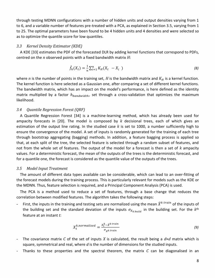
through testing MDNN configurations with a number of hidden units and output densities varying from 1

to 6, and a variable number of features pre-treated with a PCA, as explained in Section ‎3.5, varying from 1

to 25. The optimal parameters have been found to be 4 hidden units and 4 densities and were selected so

as to optimize the quantile score for low quantiles.

3.3 Kernel Density Estimator (KDE)

A KDE [33] estimates the PDF of the forecasted DLR by adding kernel functions that correspond to PDFs,

centred on the n observed points with a fixed bandwidth matrix H:

( )

∑ ( ) (8)

where n is the number of points in the training set, H is the bandwidth matrix and is a kernel function.

The kernel function is here selected as a Gaussian one, after comparing a set of different kernel functions.

The bandwidth matrix, which has an impact on the model’s performance, is here defined as the identity

matrix multiplied by a factor , set through a cross-validation that optimizes the maximum

likelihood.

3.4 Quantile Regression Forest (QRF)

A Quantile Regression Forest [34] is a machine-learning method, which has already been used for

ampacity forecasts in [20]. The model is composed by k decisional trees, each of which gives an

estimation of the output line rating. In the studied case k is set to 1000, a number sufficiently high to

ensure the convergence of the model. A set of inputs is randomly generated for the training of each tree

through bootstrap aggregating (bagging) methods. In addition, a feature bagging process is applied so

that, at each split of the tree, the selected feature is selected through a random subset of features, and

not from the whole set of features. The output of the model for a forecast is then a set of k ampacity

values. For a deterministic forecast, the mean of the outputs of the trees is the deterministic forecast, and

for a quantile one, the forecast is considered as the quantile value of the outputs of the trees.

3.5 Model Input Treatment

The amount of different data types available can be considerable, which can lead to an over-fitting of

the forecast models during the training process. This is particularly relevant for models such as the KDE or

the MDNN. Thus, feature selection is required, and a Principal Component Analysis (PCA) is used.

The PCA is a method used to reduce a set of features, through a base change that reduces the

correlation between modified features. The algorithm takes the following steps:

- First, the inputs in the training and testing sets are normalized using the mean of the inputs of

the building set and the standard deviation of the inputs in the building set. For the kth

feature at an instant t:

(9)

- The covariance matrix C of the set of inputs X is calculated, the result being a d×d matrix which is

square, symmetrical and real, where d is the number of dimensions for the studied inputs.

- Thanks to these properties and the spectral theorem, the matrix C can be diagonalised in an

9

orthonormal base. A set of eigenvalues and eigenvectors is obtained.

- The different eigenvectors can then be ranked with the eigenvalues, the highest one being associated

with a vector on which the projection of the inputs will have a higher variance than on the other one.

- A projection of the inputs on the different eigenvectors is made, and a limited number of the new

features are selected, in accordance with their ranking obtained with the eigenvalues.

The method is run to provide a set of data with ranked features, and it is possible to estimate how the

number of features of the inputs influences the different models.

4 TEST CASE

4.1 Data

To evaluate the forecasting capabilities of the models presented in Section ‎3 for the specific problem of

DLR forecasting, the following test case is considered.

The data used come from a 110kV line equipped with a 175 mm² Lynx conductor, with a maximum core

temperature set at 75°C. Weather data measurements are available for 8 weather stations installed on

the line with a time step of 5 minutes and covering a period of 2 years (2009-2010). The recorded weather

variables for each station include wind speed (m.s-1), wind direction (degrees), global solar irradiation

(W.m-2) and ambient temperature (°C).

Historical NWPs from ECMWF are considered covering the same period and location as the

measurements. NWPs are provided every 12 hours for horizons up to 48 hours, with a time step of 3

hours and a spatial resolution of 0.125°. The variables considered include the 10 m zonal and meridional

wind components (m.s-1), solar global solar irradiation (W.m-2) and ambient temperature (°C).

The forecasts are made in different positions from the weather observation recordings. Each station of

the studied cases uses the four closest points on the weather forecast grid.

The use of the different data sources mentioned can be summarised as follows: Firstly historic weather

station records are averaged over a period of 15 minutes and used to calculate historic values of RTLR for

each time t. Then historic NWP provide information about the weather forecasted time t. Since NWP have

a three-hour time resolution, far lower than the 15 minutes of the averaged weather station records,

NWPs have been interpolated linearly in order to have the same number of couples RTLR and NWP for

each time t. These couples of values are then used for training the models, with RTLR and NWP at time t

being equal to the terms and found in models description from Equation (2) to Equation (8).

4.2 Critical Section of the Line

RTLR is a parameter variable along a circuit and potentially could be calculated or measured for every

span. This is because of circuit orientation, soil roughness and eventual shielding by other objects. This is

reflected also in RTLR forecast and hence in DLR selection.

In order to take this fact into account, several solutions are possible. A first approach is to identify

critical spans on a line and then measure or calculate RTLR in this point. The critical span could potentially

change over time due to weather condition, mainly wind direction. Solutions for identifying critical spans

are suggested in [35], [36] and [37]. A second approach is represented by measuring or calculating RTLR

along all the spans or a large number of spans on the line and then assumes that the minimum value at

each time stamp corresponds to the RTLR of the line. Once the RTLR of the line has been defined and over

10

the historical training period, it can be used to calculate RTLR forecasts and set the DLR of the line.

However, for generalisation purposes in this study RTLR has been calculated and forecasted for each

different measurement point on the line, allowing the use of 8 times more data for calculating the

performance of the forecast models.

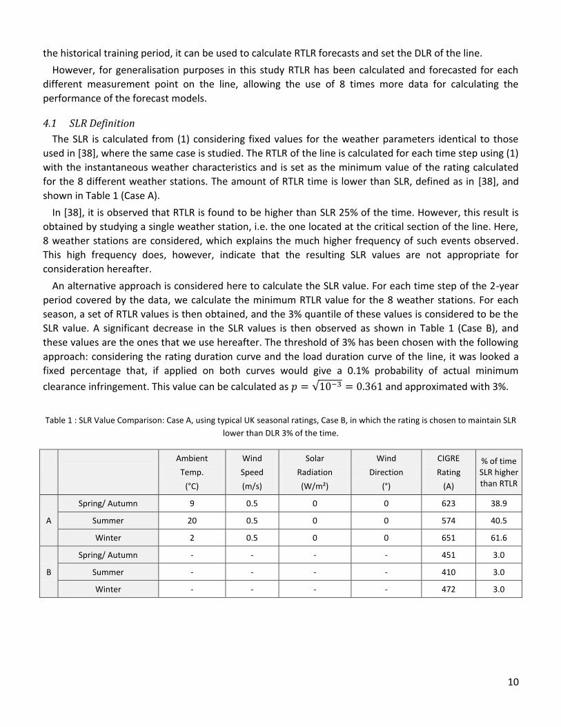
4.1 SLR Definition

The SLR is calculated from (1) considering fixed values for the weather parameters identical to those

used in [38], where the same case is studied. The RTLR of the line is calculated for each time step using (1)

with the instantaneous weather characteristics and is set as the minimum value of the rating calculated

for the 8 different weather stations. The amount of RTLR time is lower than SLR, defined as in [38], and

shown in Table 1 (Case A).

In [38], it is observed that RTLR is found to be higher than SLR 25% of the time. However, this result is

obtained by studying a single weather station, i.e. the one located at the critical section of the line. Here,

8 weather stations are considered, which explains the much higher frequency of such events observed.

This high frequency does, however, indicate that the resulting SLR values are not appropriate for

consideration hereafter.

An alternative approach is considered here to calculate the SLR value. For each time step of the 2-year

period covered by the data, we calculate the minimum RTLR value for the 8 weather stations. For each

season, a set of RTLR values is then obtained, and the 3% quantile of these values is considered to be the

SLR value. A significant decrease in the SLR values is then observed as shown in Table 1 (Case B), and

these values are the ones that we use hereafter. The threshold of 3% has been chosen with the following

approach: considering the rating duration curve and the load duration curve of the line, it was looked a

fixed percentage that, if applied on both curves would give a 0.1% probability of actual minimum

clearance infringement. This value can be calculated as √ and approximated with 3%.

Table 1 : SLR Value Comparison: Case A, using typical UK seasonal ratings, Case B, in which the rating is chosen to maintain SLR

lower than DLR 3% of the time.

Ambient

Temp.

(°C)

Wind

Speed

(m/s)

Solar

Radiation

(W/m²)

Wind

Direction

(°)

CIGRE

Rating

(A)

% of time SLR higher than RTLR

A

Spring/ Autumn 9 0.5 0 0 623 38.9

Summer 20 0.5 0 0 574 40.5

Winter 2 0.5 0 0 651 61.6

B

Spring/ Autumn - - - - 451 3.0

Summer - - - - 410 3.0

Winter - - - - 472 3.0

11

5 RESULTS - MODEL EVALUATION

Simulations have been run with the four models described in order to quantify their performance. An example of the day-ahead DLR forecast over a period of four days is shown in Fig. 2. The figure shows probability intervals in shades of blue and observations in red. The white area below the lightest blue represents values with a 1% probability of occurrence.

Fig. 2. Example of the RTLR probabilistic forecast over a four days period with the QRF model.

5.1 Evaluation criteria

5.1.1 Feature and Model Parameter Selection Method

The data used to train the models are a mix of weather station observations and NWPs. DLR forecasts

are made for the point on the line where the weather station is located. The following 24 types of data

are considered as possible model inputs:

- Observations of the 4 available weather variables at time t at the position of the weather station.

- Observed values of RTLR at time t and t-1.

- Observed values of RTLR at t+h-k, where k=24 or 48 hours, depending on whether h>24 hours or not.

NWPs of the 4 weather variables for t+h for each of the 4 closest grid points of the weather model

around the weather station are also considered.

Given the quite high number of possible inputs, a feature selection is necessary in order to avoid

overfitting and guarantee that the models have good generalization capacity. This is done through a

transformation with a PCA and the provided ranking of the newly obtained features. Then, for each

model, the evolution of a statistical criterion as a function of the number of features is computed, and the

optimal number of features is set at the value that optimizes the considered criterion. Two criteria are

used: the Continuous Ranked Probability Score (CRPS), which evaluates the ability of the model to provide

a good density forecast, and Quantile Scores (QS), which evaluate the ability of the model to provide a

good quantile forecast. This method is applied to all considered models except the QRF, for which no

feature selection is made since the use of the PCA would imply a degradation of the model’s

performances due to the feature bagging process used by the model itself.

06/05/2010 07/05/2010 08/05/2010 09/05/2010 10/05/2010

0

200

400

600

800

1000

1200

1400

06/05/2010 07/05/2010 08/05/2010 09/05/2010 10/05/2010

Am

pac

ity

[A]

Time [dd/mm/yyyy]

98% int. 80% int. 60% int. 40% int. 20% int. obs

12

5.1.2 Selection Based on the CRPS Score

The Continuous Ranked Probability Score (CRPS) is a criterion commonly used to evaluate probabilistic

forecasts:

( ) ∫ ( ( ) )

(10)

where:

( ) ∫ ( )

(11)

The CRPS, as calculated for 24-hour-ahead forecasts made for each model using as input a number of

features varying from 1 to 24, is shown in the top part of Fig. 3. The number of features corresponds to

the ranking ascertained from the PCA analysis. We observe that all 3 models and MDNN models reach

their optimum with a low number of selected features. The MDNN appears less sensitive to the number

of features. As expected, the KDE model appears to be sensitive to over-fitting, while this is less the case

for the MDNN and the QLR.

5.1.3 Selection Based on the QS Score

The CRPS provides an evaluation of the entire density forecast provided by a probabilistic forecast

model. However, for DLR forecasts, high quantiles must not be used, and so their quality should weigh

less in the evaluation of the forecast models. An approach focused on evaluating the low quantiles is thus

preferred and so a Quantile Score (QS) is defined that corresponds to the cost function, which is

minimized in the case of the QLR model:

∑ (

)

(12)

where:

( ) {

( ) (13)

It must be stressed that the CRPS is equivalent to the integral of the QS for all probability going from 0

to 100%. Due to the fact that different low quantiles could be used in practical applications, we calculate

the mean value of the quantile scores for the 10 quantiles from 1% to 10%. As for the CRPS, the value of

this average QS is calculated for the different models at a horizon of 24 hours ahead and with a different

number of features, from 1 to 24, ranked through the PCA. The result is shown in the lower graph on Fig.

3.

13

Fig. 3. Comparison of the CRPS and the QS obtained with the MDNN and the KDE, with a variable number of features selected

through PCA

We observe similar results to those observed for the KDE and the QLR with the CRPS study. However, in

the case of the MDNN, while it was observed that the CRPS index was not very sensitive to the number of

features, the QS index appears to be far more sensitive to the number of features than KDE. This leads to

a final selection of 4 features for the MDNN model. No feature selection is made for the QLR.

5.2 Evaluation of Deterministic Forecasts

The four considered models are used to generate hourly forecasts for 42 hours ahead, every 12 hours,

at lead times of 00.00 and 12.00. The models are trained for each of the 8 weather stations.

The models are first evaluated for their ability to provide good deterministic forecasts obtained from

the mean values of the predicted PDFs. The Mean Absolute Percentage Error (MAPE) criterion is used for

this purpose:

∑ |

|

(14)

For comparison purposes, a “Persistence” model is used as a benchmark, the forecasts with this model

at t+h being set as equal to the observations at t.

The results are depicted in Fig. 6 (a). The QRF model performs better than the other models. It provides

14

a MAPE improvement of 28% over Persistence for 24 hours ahead. The MAPE values are similar to those

obtained in [20], where the same case study is used to provide DLR forecasts.

5.3 Evaluation of Probabilistic Forecasts

5.3.1 Reliability

The reliability of a probabilistic forecast is its ability to ensure that the nominal proportions of the

quantile forecasts are respected in practice. As an example, a reliable model would provide 90% intervals,

which contain 90% of the observations. The reliability is assessed through Probability Integral Transform

(PIT) histograms, as shown in Fig. 4, with the addition of the standard deviation of the observed results for

the 8 different stations.

Fig. 4. PIT histograms for RTLR forecast made with the 4 considered models at a horizon of 24 hours.

Due to security criteria, low quantiles are often selected in DLR forecasting applications. For this reason,

we focus on the performance of the models for the quantiles from 1% to 20%, shown in Fig. 5. In this

context, security is referred to the problem of clearance breaching or worst of contact with hearth or

objects. A very clear modelling of this is described in [39] where the risk of operating the line at a certain

rating is modelled in order to set SLR. In general, both for SLR and low quantiles in the range 1%-5% are

proposed in the literature as a solution to set ‘safe’ DLRs.

15

Fig. 5. PIT histograms for RTLR forecast made with the QRF, the KDE, the MDNN and the QLR for a 24-hour horizon.

Depending on the selected quantile, the models perform differently. For the 5% quantile, the difference

between nominal and observed coverage remains limited, even if some improvements could be made.

However, for the 1% quantile, the ratio between observed and nominal coverage can reach 400% for the

case of QLR. Relatively high volatility in the reliability of the models for different weather stations is

observed for the 1% quantile. The KDE and QRF provide the best results regarding reliability for low

quantiles, although, with a notable difference, i.e. the frequency of events observed in which the

observation is below the forecast is lower than that expected with the KDE.

5.3.2 Sharpness

The sharpness criterion is linked to the ability of a probabilistic model to predict events with extreme

probability (close to 0 or 1). It is evaluated through the interval size. Here, a 94% mean interval size is

used, i.e. the mean difference between the 3% forecasted quantile and the 97% shown in Fig. 6 (b). The

QRF outperforms the other models for horizons longer than 4 hours.

16

Fig. 6. Comparison of the evaluation criteria for the four considered models, depending on the forecast horizon.

17

5.3.3 Continuous Ranked Probability Score (CRPS)

To select models with an optimal balance between sharpness and reliability, several scores are proposed

in the literature. Here, the CRPS score, described above, is considered. This score can be used to evaluate

the entire distribution and is equivalent to the mean absolute error used for deterministic forecast

evaluation, the results being the same for the case of a distribution assimilated to a Dirac function. The

results shown in Fig. 6 (c) indicate that the QRF outperforms the other models, which implies that this is

the best model to consider the entire distribution rather than specific quantiles.

5.3.4 Quantile Score (QS)

As mentioned above, DLR forecasts require low quantiles, and so a focus is put here on the Quantile

Score. The average value of the QS score for the 10 quantiles from 1% to 10% is used, and the results are

shown in Fig. 6 (d). The QRF outperforms the other models on this criterion. It should be noted that the

distribution tail was modelled with the same model that was used to forecast the entire distribution.

However, the quantiles below 5% could have been modelled in line with the Extreme Value Theory (EVT),

where the tail provided by the initial model could be replaced with a new tail with characteristics defined

in accordance with the EVT. This option is considered in the perspectives of this work.

5.3.5 Conclusion

The analysis of the performance of the four models considered shows that QRF outperforms all other

models in all metrics. Anyway, it must be noted that the most important indicator for the application

described further in Section 6 is the PIT diagram for very low quantiles (1%-5%). For this indicator and in

this range its performance is not very far from the MDDN model, with the difference that this second

model tends to underestimate low-value forecast with potentially higher risk in operation. In summary,

the QRF model results in the best one according to the metrics considered. This will be further analysed

below when a specific application of RTLR forecasts for selecting day-ahead DLR is proposed and

evaluated. Regarding the computational time and resources used for forecasts, they have not been found

excessive of problematic for deployment: tests have been done on a desktop with a 3.15 GHz processor

and a 16GB RAM, training time for a forecast model is in the order of minutes whilst the day ahead

forecast is performed in fractions of second.

6 RTLR FORECAST APPLICATION

6.1 Description of the problem

From a physical point of view, the current-carrying capacity of overhead line conductors is determined by the maximum sag able to guarantee the minimum allowed clearance. Conductors lose tensile strength and therefore increase their sag with an increase in temperature, as summarized in Equation (15) with the link between tensile strength and vertical sag and (16) with the relation between conductor temperature and axial tensile strength.

(15)

(

)

(16)

18

where: Lsag [m] is the sag, Fp [N] is the linear weight of the conductor, Ft [N] is the tensile strength of the conductor, Lspan [m] is the length of the span, Ec *Pa+ is the Young’s modulus, Ac [m

2] is the conductor’s cross-sectional area, βc [K-1+ is the conductor’s thermal expansion factor, and Tc,i *K+ is the conductor’s temperature at time i. Further details can be found in [40].

When a new line is designed, its economical optimization partly depends on its tensioning, span length and operating and maximum temperatures (which also influence the annealing and life of the circuit).

6.1.1 Fixed quantile (FQ) strategy

The selected DLR should not be less safe than the SLR, therefore a first strategy to select DLR is to consistently choose a quantile that corresponds to an exceedance probability equal to the SLR temperature-exceedance probability already applied on the line. For example, if for a circuit the observed ampacity is below the SLR 4% of the time, then it is possible to set the DLR at the 4% quantile of the forecast.

6.1.2 Accepted risk (AR) strategy

The AR strategy proposed is based on a quantification of the risk associated with the exceedance of minimum clearances expected on a conductor. It is based on the following assumptions:

- If a live conductor enters in contact with the ground, there are two main costs to take into account, i.e. the electric power flow will be interrupted, with potential repercussions on the security of load supply of the loads (C1), and on the contact area, damage may be done to objects or people (C2).

- If the operating temperature exceeds the design temperature, annealing will accelerate, thus accelerating the ageing of the conductor (C3)

- Although the increase in the sag is not automatically associated with a contact, the probability of contact (Pc) will increase with the sag and with the reduction of the distance to the objects.

- When selecting DLR, the objective should not be to minimize the risk but to operate the line with an accepted level of risk (RKt).

Analytically the problem is to find the solution to Equation (17):

∫ ( )

(17)

where RK(I) is the function describing the risk in a function of the rating I as described in Equation (22).

Due to the high non-linearity and discrete structure of part of the problem, an analytical solution is not possible without introducing simplifications and linearization. Therefore, the following procedure has been defined for setting the DLR at each single time step.

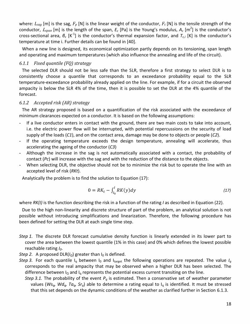
Step 1. The discrete DLR forecast cumulative density function is linearly extended in its lower part to cover the area between the lowest quantile (1% in this case) and 0% which defines the lowest possible reachable rating I0.

Step 2. A proposed DLR(IQ) greater than I0 is defined. Step 3. For each quantile Iq between I0 and Itarget the following operations are repeated. The value Iq

corresponds to the real ampacity that may be observed when a higher DLR has been selected. The difference between IQ and Iq represents the potential excess current transiting on the line. Step 3.1. The probability of the event Pq is estimated. Then a conservative set of weather parameter

values (Wsq, Wdq, Taq, Srq) able to determine a rating equal to Iq is identified. It must be stressed that this set depends on the dynamic conditions of the weather as clarified further in Section ‎6.1.3.

19

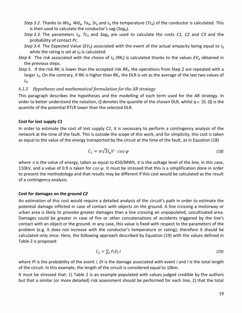
Step 3.2. Thanks to Wsq, Wdq, Taq, Srq and IQ the temperature (Tcq) of the conductor is calculated. This is then used to calculate the conductor’s sag (Sagq).

Step 3.3. The parameters IQ, Tcq and Sagq are used to calculate the costs C1, C2 and C3 and the probability of contact Pc.

Step 3.4. The Expected Value (EVq) associated with the event of the actual ampacity being equal to Iq while the rating is set at IQ is calculated.

Step 4. The risk associated with the choice of IQ (RKI) is calculated thanks to the values EVq obtained in the previous steps.

Step 5. If the risk RKI is lower than the accepted risk RKt, the operations from ‎Step 2 are repeated with a larger IQ. On the contrary, if RKI is higher than RKt, the DLR is set as the average of the last two values of IQ.

6.1.3 Hypotheses and mathematical formulation for the AR strategy

This paragraph describes the hypotheses and the modelling of each term used for the AR strategy. In

order to better understand the notation, Q denotes the quantile of the chosen DLR, whilst q [0, Q] is the quantile of the potential RTLR lower than the selected DLR.

Cost for lost supply C1

In order to estimate the cost of lost supply C1, it is necessary to perform a contingency analysis of the network at the time of the fault. This is outside the scope of this work, and for simplicity, this cost is taken as equal to the value of the energy transported by the circuit at the time of the fault, as in Equation (18)

√ (18)

where is the value of energy, taken as equal to €50/MWh, V is the voltage level of the line, in this case, 110kV, and a value of 0.9 is taken for . It must be stressed that this is a simplification done in order to present the methodology and that results may be different if this cost would be calculated as the result of a contingency analysis.

Cost for damages on the ground C2

An estimation of this cost would require a detailed analysis of the circuit’s path in order to estimate the potential damage inflicted in case of contact with objects on the ground. A line crossing a motorway or urban area is likely to provoke greater damages than a line crossing an unpopulated, uncultivated area. Damages could be greater in case of fire or other concatenations of accidents triggered by the line’s contact with an object or the ground. In any case, this value is fixed with respect to the parameters of the problem (e.g. it does not increase with the conductor’s temperature or rating); therefore it should be calculated only once. Here, the following approach described by Equation (19) with the values defined in Table 2 is proposed:

∑ (19)

where Pi is the probability of the event i, Di is the damage associated with event i and l is the total length of the circuit. In this example, the length of the circuit is considered equal to 10km.

It must be stressed that: 1) Table 2 is an example populated with values judged credible by the authors but that a similar (or more detailed) risk assessment should be performed for each line, 2) that the total

20

sum of all the probabilities in the second column must be equal to 100% and 3) that in this model the Cost C2 is constant and not depending on the rating, the load or other dynamic conditions of the system.

Table 2: Risk table related to a conductor contact with the ground

Damage [€/m] Probability [%] Event

0 83.89% no damage

104 10.00% vegetation, fire

106 5.00% vegetation, extensive fire

105 1.00% object, limited damage

106 0.10% object, damage

108 0.01% object, extensive damage

107 0.001% People

Cost of conductor ageing C3

Precise models have been defined for calculating the effect of annealing on overhead conductors and the reader is referred to [39], [41]and [42] for more information. In the case of Aluminium Conductor Steel Reinforced (ACSR) conductors, annealing is a minor problem since most of the mechanical load is supported by the steel core, which does not anneal for temperatures up to 200°C. For this reason, a simple cost function has been used here to penalize higher temperatures:

{

(20)

where has been estimated at 50 k€/km. It must be stressed that this event and these

temperatures are relative only to very large faults and are not relative to the normal operating conditions of the line where the problem is creep over years.

Probability of contact Pc

The probability of contact is expected to tend to zero if the conductor’s sag is within its design level, and to tend to 100% if the conductor’s sag is as great as the minimum clearance value. The law connecting these two extremes is not known and no studies have been carried out on this. In this work, it is modelled as a power function as reported in Equation (21):

(( )

)

(21)

where h is the minimum clearance, set as 10m in this test, Lsag and Lsag,d are respectively the sag and the design sag, and a is the exponent, set as 1.25. The lowest is the value of the exponent a, the highest is the security considered. This value has been calculated by imposing that the expected risk relative to SLR B should be of 0.5 €/MVA/km in the climatic conditions considered. It must be clarified anyway that this value should be defined from a risk assessment of the environment of the line and a proper methodology must still be developed for this.

Accepted risk RKt

21

The risk is defined as the product between the damage (Di) associated with an event i and the probability (Pi) of the event’s occurrence, as shown in Equation (22). For clarity, this has been made dimensionless with MVA rating of the line when the SLR is applied.

√ (22)

Therefore, it can be expressed in terms of the cost per hour of operating the line. When the rating of the line is set, in the case of DLR or of traditional SLR, a certain value of risk is implicitly accepted.

In this work, an accepted risk of 0.5 €MVA-1km-1 is taken as a reference, although a sensitivity analysis is

carried out for values of risk ranging from 0.1 to 1 5 €MVA-1km-1. This value has been chosen considering

the cost of insurance necessary to waive the risk, and at a cost equivalent to 1‰ of the value of the energy flowing on the line at a value equal to the static rating.

Modeling the tail of the distribution and I0

Also, in this case, no work has been done on modelling the lowest part of a distribution of RTLR values.

In this work, it has been chosen to model the distribution tail employing a linear interpolation between Iqmin and I0, with a step equal to 0.1%. Iqmin is the rating of the minimum quantile available from the probabilistic forecast, in this case, 1%.

I0 is calculated with the following method: the database of meteorological records related to the area is searched for the time steps relative to the same month and the same hour (but for all the available years) of the time step in question. The most conservative values are taken, corresponding to the minimum recorded wind speed (Wst,min) and the maximum recorded air temperature (Tat,min) and solar radiation (Srt,min). Wind direction is taken as equal to 10°, almost parallel to the axis of the conductor, and the resulting ampacity is then calculated with these values.

This method can be used to take into account location-specific weather conditions, along with seasonal and daily variations, whilst considering extreme conditions, since the correlation between the weather parameters is not taken into account.

Probability of event Pq

The probability of an event associated with a rating that has a value of Iq is calculated as the difference between the value of the probability at step q and step q-1.

This should be multiplied by the probability of having a power flow above the value Iq at the specific time step. This is not considered in this work, and thus to make a very conservative assumption this probability is set at 100%.

Conservative set of weather parameters (Wsq, Wdq, Taq, Srq)

This is a problem that can be solved in different ways and presents several equivalent solutions since different combinations of the weather parameters can produce the same rating value. The approach chosen here is described below.

As seen for the estimation of I0, the weather records relative to the same hour and the same calendar month (but for all the available years) of the time step in question are selected and sorted into a descending order for wind speed, solar radiation and air temperature. Wind direction is always considered as equal to 10°. At this point, the records are scanned and an ampacity is calculated as in

22

Equation (1) with the different sets of parameters. When the calculated current is equal to Iq, the value of the weather parameters used is chosen to represent Wsq, Wdq, Taq, Srq.

Conductor temperature Tcq

The conductor temperature for a given current flowing in the conductor is calculated thanks to Equation (1).

Conductor sag Sagq

The conductor sag is calculated thanks to Equation (15) and (16) considering the conductor current calculated as described above. Regarding reference conditions, it is considered that the conductor has been tensioned at 20% of its rated strength [43]

Expected value of the damage EVq

The expected value of the cost associated with the event of having set the DLR to the value IQ whilst its real limit is Iq can be calculated as shown in Equation (23).

( ( ))

√ (23)

This means that the cost associated with the annealing must be weighted with the probability of the occurrence of the event, whilst the cost associated with the contact must also be weighted with the probability of the conductor touching the ground or an object.

Risk for selected DLR RKI

Finally, the total risk associated with setting the rating at the value IQ is calculated as the integral of the expected value associated with all of the events of the actual rating, Iq being smaller than IQ as shown in Equation (24).

∫ ( )

(24)

6.2 Results and comparison

The AR strategy described in Section ‎6 has been applied for growing values of the accepted risk of 0.25,

0.5 and 1 €MVA-1km-1. This is compared with the FQ strategy for quantiles ranging from 1% to 10% and

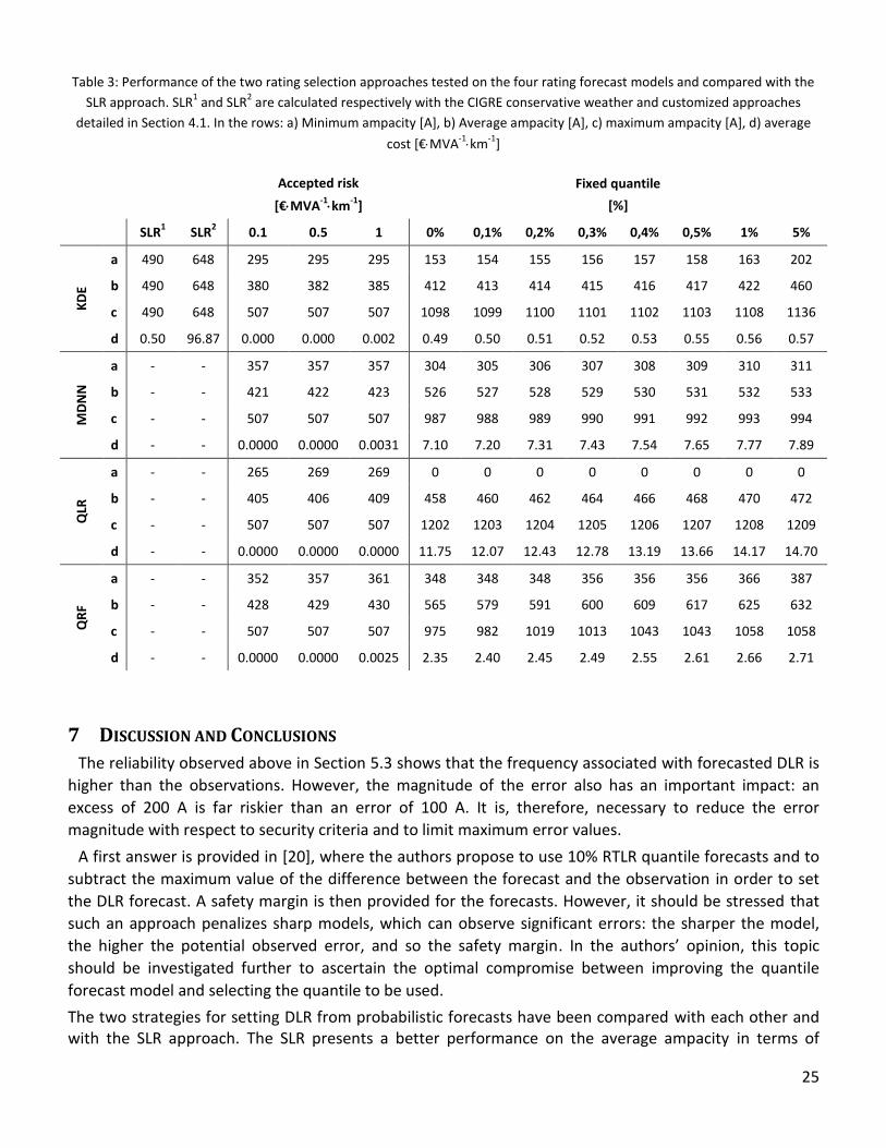
with the traditional SLR strategy. This is repeated for the four forecast algorithms developed. The DLR calculated for the two strategies and the four models were then used to simulate the behaviour of the sag and hence the risk of operating the line with the selected DLR, considering the observed weather conditions and a current flowing on the line equal to the DLR. The results are reported in Fig. 7 and Table 3 where for each strategy and for each forecast model key metrics are reported. In Fig. 7 the best solutions are located at the bottom right of the chart, where a high average DLR corresponds to low operating risk. The values of the risk presented in this chart are particularly high, but this is normal since they are calculated considering a current that is always equal to the DLR applied, whilst in reality, the probability of such an event is very low.

23

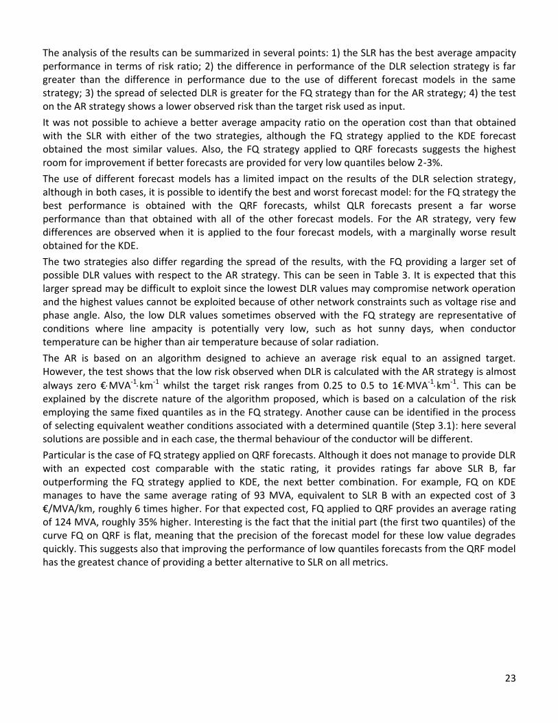
The analysis of the results can be summarized in several points: 1) the SLR has the best average ampacity performance in terms of risk ratio; 2) the difference in performance of the DLR selection strategy is far greater than the difference in performance due to the use of different forecast models in the same strategy; 3) the spread of selected DLR is greater for the FQ strategy than for the AR strategy; 4) the test on the AR strategy shows a lower observed risk than the target risk used as input.

It was not possible to achieve a better average ampacity ratio on the operation cost than that obtained with the SLR with either of the two strategies, although the FQ strategy applied to the KDE forecast obtained the most similar values. Also, the FQ strategy applied to QRF forecasts suggests the highest room for improvement if better forecasts are provided for very low quantiles below 2-3%.

The use of different forecast models has a limited impact on the results of the DLR selection strategy, although in both cases, it is possible to identify the best and worst forecast model: for the FQ strategy the best performance is obtained with the QRF forecasts, whilst QLR forecasts present a far worse performance than that obtained with all of the other forecast models. For the AR strategy, very few differences are observed when it is applied to the four forecast models, with a marginally worse result obtained for the KDE.

The two strategies also differ regarding the spread of the results, with the FQ providing a larger set of possible DLR values with respect to the AR strategy. This can be seen in Table 3. It is expected that this larger spread may be difficult to exploit since the lowest DLR values may compromise network operation and the highest values cannot be exploited because of other network constraints such as voltage rise and phase angle. Also, the low DLR values sometimes observed with the FQ strategy are representative of conditions where line ampacity is potentially very low, such as hot sunny days, when conductor temperature can be higher than air temperature because of solar radiation.

The AR is based on an algorithm designed to achieve an average risk equal to an assigned target. However, the test shows that the low risk observed when DLR is calculated with the AR strategy is almost

always zero €MVA-1km-1 whilst the target risk ranges from 0.25 to 0.5 to 1€MVA-1

km-1. This can be explained by the discrete nature of the algorithm proposed, which is based on a calculation of the risk employing the same fixed quantiles as in the FQ strategy. Another cause can be identified in the process of selecting equivalent weather conditions associated with a determined quantile (Step 3.1): here several solutions are possible and in each case, the thermal behaviour of the conductor will be different.

Particular is the case of FQ strategy applied on QRF forecasts. Although it does not manage to provide DLR with an expected cost comparable with the static rating, it provides ratings far above SLR B, far outperforming the FQ strategy applied to KDE, the next better combination. For example, FQ on KDE manages to have the same average rating of 93 MVA, equivalent to SLR B with an expected cost of 3 €/MVA/km, roughly 6 times higher. For that expected cost, FQ applied to QRF provides an average rating of 124 MVA, roughly 35% higher. Interesting is the fact that the initial part (the first two quantiles) of the curve FQ on QRF is flat, meaning that the precision of the forecast model for these low value degrades quickly. This suggests also that improving the performance of low quantiles forecasts from the QRF model has the greatest chance of providing a better alternative to SLR on all metrics.

24

Fig. 7: Average power transfer and risk for different DL strategies compared with SR. The lowest chart magnifies the region up

to 5 €MVA-1km

-1

0

20

40

60

80

100

Ave

rage

exp

ecte

d c

ost

[€

/MV

A/k

m]

KDE Fixed Risk MDNN Fixed Risk QLR Fixed Risk QRF Fixed Risk KDE Fix Q

MDNN Fix Q QLR Fix Q QRF Fix Q SLR 21% SLR 3%

0.0

1.0

2.0

3.0

4.0

5.0

60 70 80 90 100 110 120 130 140

Ave

rage

exp

ect

ed c

ost

[€

/MV

A/k

m]

Average rating [MVA]

25

Table 3: Performance of the two rating selection approaches tested on the four rating forecast models and compared with the

SLR approach. SLR1 and SLR

2 are calculated respectively with the CIGRE conservative weather and customized approaches

detailed in Section ‎4.1. In the rows: a) Minimum ampacity [A], b) Average ampacity [A], c) maximum ampacity [A], d) average

cost *€MVA-1km

-1]

Accepted risk

[€MVA-1km

-1]

Fixed quantile

[%]

SLR1 SLR

2 0.1 0.5 1 0% 0,1% 0,2% 0,3% 0,4% 0,5% 1% 5%

KD

E

a 490 648 295 295 295 153 154 155 156 157 158 163 202

b 490 648 380 382 385 412 413 414 415 416 417 422 460

c 490 648 507 507 507 1098 1099 1100 1101 1102 1103 1108 1136

d 0.50 96.87 0.000 0.000 0.002 0.49 0.50 0.51 0.52 0.53 0.55 0.56 0.57

MD

NN

a - - 357 357 357 304 305 306 307 308 309 310 311

b - - 421 422 423 526 527 528 529 530 531 532 533

c - - 507 507 507 987 988 989 990 991 992 993 994

d - - 0.0000 0.0000 0.0031 7.10 7.20 7.31 7.43 7.54 7.65 7.77 7.89

QLR

a - - 265 269 269 0 0 0 0 0 0 0 0

b - - 405 406 409 458 460 462 464 466 468 470 472

c - - 507 507 507 1202 1203 1204 1205 1206 1207 1208 1209

d - - 0.0000 0.0000 0.0000 11.75 12.07 12.43 12.78 13.19 13.66 14.17 14.70

QR

F

a - - 352 357 361 348 348 348 356 356 356 366 387

b - - 428 429 430 565 579 591 600 609 617 625 632

c - - 507 507 507 975 982 1019 1013 1043 1043 1058 1058

d - - 0.0000 0.0000 0.0025 2.35 2.40 2.45 2.49 2.55 2.61 2.66 2.71

7 DISCUSSION AND CONCLUSIONS

The reliability observed above in Section ‎5.3 shows that the frequency associated with forecasted DLR is

higher than the observations. However, the magnitude of the error also has an important impact: an

excess of 200 A is far riskier than an error of 100 A. It is, therefore, necessary to reduce the error

magnitude with respect to security criteria and to limit maximum error values.

A first answer is provided in [20], where the authors propose to use 10% RTLR quantile forecasts and to

subtract the maximum value of the difference between the forecast and the observation in order to set

the DLR forecast. A safety margin is then provided for the forecasts. However, it should be stressed that

such an approach penalizes sharp models, which can observe significant errors: the sharper the model,

the higher the potential observed error, and so the safety margin. In the authors’ opinion, this topic

should be investigated further to ascertain the optimal compromise between improving the quantile

forecast model and selecting the quantile to be used.

The two strategies for setting DLR from probabilistic forecasts have been compared with each other and with the SLR approach. The SLR presents a better performance on the average ampacity in terms of

26

average risk ratio and is not equalled by the use of the FQ strategy with the QRF forecast model, the combination with the best performances among the tested ones.

An analysis of the results and of the methodology leads to a second observation regarding the AR strategy. The risk is estimated considering a continuous power flow equal to the DLR assigned to the line, but in real life, loads are usually far lower. Therefore a strategy that also takes into account a time-dependent power-flow probabilistic forecast may obtain better performances in terms of both risk reduction and average ampacity increase. Furthermore, in both strategies, the quantiles chosen are in the lowest part of the distribution (<10%) and thus better modelling of this region is likely to improve the performance of the two strategies proposed. A final observation is related to the risk model used: it is particularly sensitive to the estimation of the damage associated with a contact, and to the probability function linking the sag to the contact; however, these two aspects have seldom been treated in research on overhead line ampacity estimations, and further work should be carried out in this area.

In conclusion: deterministic forecasts are inadequate for DLR applications, due to strict constraints

regarding current risks greater than the real-time ampacity of the line. In this context, probabilistic

forecasts appear to be a solution, and more precisely low quantile forecasts, which significantly reduce

such risks.

In this study, four models for DLR forecasting were presented. They were fitted with both NWP and

ground observations of weather variables, such inputs being suitable for forecast horizons greater than 6

hours. The models compared include QLR, QRF, MDDN and KDE. They were compared for their ability to

provide both deterministic and probabilistic forecasts, which would be reliable and compelling in terms of

ampacity gains. The advantages of considering the QS score for selecting a model was outlined.

The study highlighted the variations in the performance of the models as a function of the different

evaluation criteria. The QLR model can in principle be discarded since it underperformed on all criteria.

Regarding the remaining models, no single model outperformed on all criteria. In terms of the specific

application, the models can be ranked in line with their performance on the QS score for low quantiles.

Based on this, the QRF appears to be the most suitable for implementation.

The study also presents a description of two possible strategies for selecting day-ahead DLR using the

forecasts developed. Both cases don’t manage to achieve a considerable reduction in the risk of line

operation with respect to the application of SLR. The FQ strategy presents a higher value for the risk on

average ampacity ratio, but a wider spread of selected DLR. The AR strategy presents a very low value of

the same ratio, but with a narrower spread of potential DLRs, lower on average than the SLR. Among the

eight possible combinations tested, two strategies proved to have high potential: FQ DLR selection

strategy coupled with KDE and QRF RTLR forecasts. Unfortunately, none of these two strategies could

provide both higher average ratings and lower operational risk than SLR, showing the need for more work

on this topic.

Future areas of research opened by this work include the development of alternative forecasting

methods, i.e. based on Extreme Value Theory for modelling the tails of the forecasted PDF, or the use of

ensemble NWPs as input. Also, the DLR selection strategy could be improved considering a line’s power

flow probabilistic forecasts, or a combination of the two strategies, aiming at reducing extreme values for

the proposed DLR. Finally, a detailed evaluation of financial or other benefits would facilitate the

application of DLR forecasts by grid operators. To this end, a new methodology to evaluate DLR forecast

models could be developed, adapted to the grid operator’s objectives.

27

ACKNOWLEDGEMENT

The authors would like to thank NIE Networks (Northern Ireland Electricity Networks) and the European Centre for Medium-Range Weather Forecasts (ECMWF) for the provision of the data used in this work.

REFERENCES

[1] RTE, Bilan Prévisionnel de l’équilibre offre-demande d’électricité en France. Paris, 2015.

[2] IEEE Power Engineering Society, ‘IEEE Standard for Calculating the Current-Temperature Relationship of Bare Overhead Conductors’, IEEE Corp. Off., 1993.

[3] CIGRE, ‘Thermal Behaviour of Overhead Conductors’. 2002.

[4] J. Heckenbergerova, P. Musilek, and K. Filimonenkov, ‘Assessment of seasonal static thermal ratings of overhead transmission conductors’, in 2011 IEEE Power and Energy Society General Meeting, 2011, pp. 1–8.

[5] E. Cloet, J.-L. Lilien, and P. Ferrières, ‘Experiences of the Belgian and French TSOs using the “Ampacimon” real-time dynamic rating system’, CIGRE, 2010.

[6] R. G. Olsen and K. S. Edwards, ‘A new method for real-time monitoring of high-voltage transmission-line conductor sag’, IEEE Trans. Power Deliv., vol. 17, no. 4, pp. 1142–1152, 2002.

[7] C. J. Wallnerström, Y. Huang, and L. Söder, ‘Impact from dynamic line rating on wind power integration’, IEEE Trans. Smart Grid, vol. 6, no. 1, pp. 343–350, 2015.

[8] D. M. Greenwood and P. C. Taylor, ‘Investigating the impact of real-time thermal ratings on power network reliability’, IEEE Trans. Power Syst., vol. 29, no. 5, pp. 2460–2468, 2014.

[9] J. Teh et al., ‘Prospects of Using the Dynamic Thermal Rating System for Reliable Electrical Networks: A Review’, IEEE Access, vol. 6, pp. 26765–26778, 2018.

[10] A. Michiorri et al., ‘Forecasting for dynamic line rating’, Renew. Sustain. Energy Rev., vol. 52, pp. 1713–1730, 2015.

[11] S. Uski, ‘Estimation method for dynamic line rating potential and economic benefits’, Int. J. Electr. Power Energy Syst., vol. 65, pp. 76–82, 2015.

[12] D. A. Douglas, ‘Weather-dependant versus static thermal line rating’, IEEE Trans Power Deliv, vol. 3, no. 2, pp. 742–753, 1988.

[13] S. D. Foss and R. A. Maraio, ‘Dynamic line rating in the operating environment’, IEEE Trans. Power Deliv., vol. 5, no. 2, pp. 1095–1105, 1990.

[14] D.-M. Kim, J.-M. Cho, H.-S. Lee, H.-S. Jung, and J.-O. Kim, ‘Prediction of dynamic line rating based on assessment risk by time series weather model’, in Probabilistic Methods Applied to Power Systems, 2006. PMAPS 2006. International Conference on, 2006, pp. 1–7.

[15] K. Wang, G. Sheng, and X. Jiang, ‘Risk assessment of transmission dynamic line rating based on monte carlo’, in Power Engineering and Automation Conference (PEAM), 2011 IEEE, 2011, vol. 2, pp. 398–402.

[16] I. Albizu, E. Fernandez, A. J. Mazon, K. J. Sagastabeitia, M. T. Bedialauneta, and J. G. Olazarri, ‘Overhead line rating forecasting for the integration of wind power in electricity markets’, in Clean Electrical Power (ICCEP), 2015 International Conference on, 2015, pp. 382–388.

[17] Twenties European Project, ‘Final report on NETFLEX demo’. 2013.

28

[18] A. Michiorri and P. C. Taylor, ‘Forecasting real-time ratings for electricity distribution networks using weather forecast data’, in Electricity Distribution-Part 1, 2009. CIRED 2009. 20th International Conference and Exhibition on, 2009, pp. 1–4.

[19] T. Ringelband, P. Schäfer, and A. Moser, ‘Probabilistic ampacity forecasting for overhead lines using weather forecast ensembles’, Electr. Eng., vol. 95, no. 2, pp. 99–107, 2013.

[20] J. Aznarte and N. Siebert, ‘Dynamic Line Rating Using Numerical Weather Predictions and Machine Learning: a Case Study’.

[21] J. Black, J. Colandairaj, S. Connor, and B. O’Sullivan, ‘Equipment and methodology for the planning and implementation of dynamic line ratings on overhead transmission circuits’, in Modern Electric Power Systems (MEPS), 2010 Proceedings of the International Symposium, 2010, pp. 1–6.

[22] A. McLaughlin, M. Alshamali, J. Colandairaj, and S. Connor, ‘Application of dynamic line rating to defer transmission network reinforcement due to wind generation’, in Universities’ Power Engineering Conference (UPEC), Proceedings of 2011 46th International, 2011, pp. 1–6.

[23] J. Fu, D. J. Morrow, and S. M. Abdelkader, ‘Modelling and prediction techniques for dynamic overhead line rating’, in 2012 IEEE Power and Energy Society General Meeting, 2012, pp. 1–7.

[24] D. J. Morrow, J. Fu, and S. M. Abdelkader, ‘Experimentally validated partial least squares model for dynamic line rating’, IET Renew. Power Gener., vol. 8, no. 3, pp. 260–268, 2014.

[25] J. Fu, S. Abbott, B. Fox, D. J. Morrow, and S. Abdelkader, ‘Wind cooling effect on dynamic overhead line ratings’, in Universities Power Engineering Conference (UPEC), 2010 45th International, 2010, pp. 1–6.

[26] F. Fan, K. Bell, and D. Infield, ‘Probabilistic Real-Time Thermal Rating Forecasting for Overhead Lines by Conditionally Heteroscedastic Auto-Regressive Models’, IEEE Trans. Power Deliv., vol. 32, no. 4, pp. 1881–1890, Aug. 2017.

[27] J. Zhan, C. Y. Chung, and E. Demeter, ‘Time Series Modeling for Dynamic Thermal Rating of Overhead Lines’, IEEE Trans. Power Syst., vol. 32, no. 3, pp. 2172–2182, May 2017.

[28] M. A. Bucher, M. Vrakopoulou, and G. Andersson, ‘Probabilistic N−1 security assessment incorporating dynamic line ratings’, in 2013 IEEE Power Energy Society General Meeting, 2013, pp. 1–5.

[29] R. Dupin, A. Michiorri, and G. Kariniotakis, ‘Dynamic line rating day-ahead forecasts - cost benefit based selection of the optimal quantile’, in CIRED 2016 workshop - Electrical networks for society and people, Helsinki, Finland, 2016.

[30] R. Koenker and G. Bassett Jr, ‘Regression quantiles’, Econom. J. Econom. Soc., pp. 33–50, 1978.

[31] C. M. Bishop, ‘Mixture density networks’, 1994.

[32] J. Carreau and M. Vrac, ‘Stochastic downscaling of precipitation with neural network conditional mixture models’, Water Resour. Res., vol. 47, no. 10, 2011.

[33] D. W. Scott, Multivariate density estimation: theory, practice, and visualization. John Wiley & Sons, 2015.

[34] N. Meinshausen, ‘Quantile regression forests’, J. Mach. Learn. Res., vol. 7, no. Jun, pp. 983–999, 2006.

[35] I. Cotton and J. Teh, ‘Critical span identification model for dynamic thermal rating system placement’, IET Gener. Transm. Distrib., vol. 9, no. 16, pp. 2644–2652, Dec. 2015.

29

[36] M. Matus et al., ‘Identification of Critical Spans for Monitoring Systems in Dynamic Thermal Rating’, IEEE Trans. Power Deliv., vol. 27, no. 2, pp. 1002–1009, Apr. 2012.

[37] J. W. Jerrell, W. Z. Black, and T. J. Parker, ‘Critical span analysis of overhead conductors’, IEEE Trans. Power Deliv., vol. 3, no. 4, pp. 1942–1950, Oct. 1988.

[38] J. Fu, D. J. Morrow, S. Abdelkader, and B. Fox, ‘Impact of dynamic line rating on power systems’, in Universities’ Power Engineering Conference (UPEC), Proceedings of 2011 46th International, 2011, pp. 1–5.

[39] H. Wan, J. D. McCalley, and V. Vittal, ‘Increasing thermal rating by risk analysis’, IEEE Trans. Power Syst., vol. 14, no. 3, pp. 815–828, Aug. 1999.

[40] C. R. Bayliss and B. J. Hardy, Transmission and distribution electrical engineering, 4th ed. Oxford ; Boston: Elsevier/ Newnes, 2012.

[41] V. T. Morgan, ‘Effect of elevated temperature operation on the tensile strength of overhead conductors’, IEEE Trans. Power Deliv., vol. 11, no. 1, pp. 345–352, Jan. 1996.

[42] V. Morgan, ‘The Loss of Tensile Strength of Hard-Drawn Conductors by Annealing in Servicec’, IEEE Trans. Power Appar. Syst., vol. PAS-98, no. 3, pp. 700–709, May 1979.

[43] D. Douglass and F. Thrash, ‘Sag and Tension of Conductor’, in Electric Power Generation, Transmission, and Distribution, Third Edition, vol. 20124365, CRC Press, 2012, pp. 1–42.