Embed Size (px)
Citation preview
1
Out-of-Band Millimeter Wave Beamforming andCommunications to Achieve Low Latency and High
Energy Efficiency in 5G SystemsMorteza Hashemi, Student Member, IEEE, C. Emre Koksal, Senior Member, IEEE,
and Ness B. Shroff, Fellow, IEEE
Abstract—Communications in the millimeter wave (mmWave)band faces significant challenges due to variable channels, inter-mittent connectivity, and high energy usage. Moreover, speeds forelectronic processing of data is of the same order as typical ratesfor mmWave interfaces, making the use of complex algorithms fortracking channel variations and adjusting resources impractical.In order to mitigate some of these challenges, we proposean architecture that integrates the sub-6 GHz and mmWavetechnologies. Our system exploits the spatial correlations betweenthe sub-6 GHz and mmWave interfaces for beamforming anddata transfer. Based on extensive experimentation in indoor andoutdoor settings, we demonstrate that analog beamforming canbe used in mmWave without incurring large overhead, thanksto the spatial correlations with sub-6 GHz. In addition, weincorporate the sub-6 GHz interface as a fallback (secondary)data transfer mechanism such that (i) the negative effects ofhighly intermittent mmWave connectivity is mitigated, and (ii)the abundant mmWave capacity is fully exploited. To achievethese goals, we consider the problem of scheduling the arrivaltraffic over the mmWave or sub-6 GHz in order to maximizethe mmWave throughput while delay (due to mmWave outages)is guaranteed to be bounded. We prove using subadditivityanalysis that the optimal scheduling policy is based on a singlethreshold that can be easily adopted despite high link variations.Numerical results demonstrate that our scheduler provides abounded mmWave delay performance, while it achieves a similarthroughput performance as the throughput-optimal policies (e.g.,MaxWeight).
Index Terms—Millimeter wave communication, 5G mobilesystems, Out-of-band beamforming and communication
I. INTRODUCTION
The annual data traffic generated by mobile devices isexpected to surpass 130 exabits by 2020 [1]. This delugeof traffic will significantly exacerbate the spectrum crunchthat cellular providers are already experiencing. To addressthis issue, it is envisioned that in 5G cellular systems certainportions of the mmWave band will be used, spanning thespectrum between 30 GHz to 300 GHz with the correspondingwavelengths between 1-10 mm [2]. This will substantiallyincrease the spectrum available to cellular providers, which iscurrently between 700 MHz and 2.6 GHz with only 780 MHzof bandwidth allocation for all current cellular technologies.
M. Hashemi and C. E. Koksal are with the Department of Electrical andComputer Engineering, Ohio State University, Columbus, OH, 43210 USAe-mail: [email protected], [email protected]
N. B. Shroff is with the Department of Electrical and Computer Engineeringand Department of Computer Science and Engineering, Ohio State University,Columbus, OH, 43210 USA e-mail: [email protected].
Before mmWave communications can become a reality,there are significant challenges that need to be overcome.Firstly, compared with sub-6 GHz, the propagation loss inmmWave is much higher due to atmospheric absorption andlow penetration. Although large antenna arrays have the po-tential to make up for the mmWave losses, they cause severalother issues such as high energy consumption by components(e.g., analog-to-digital converters (ADC)). For instance, at asampling rate of 1.6 Gsamples/sec, an 8−bit quantizer con-sumes ≈ 250mW of power. During active transmissions, thiswould constitute up to 50% of the overall power consumptionfor a typical smart phone. Moreover, in order to fully utilizethe large directional antenna arrays, continuous beamformingand signal training at the receiver is needed [3]. Digitalbeamforming is highly efficient in delay, but there is a need fora separate ADC for each antenna, which may not be feasiblefor even a small to mid-sized antenna array due to high energyconsumption. In contrast, analog beamforming requires onlyone ADC, but it can focus on one direction at a time, makingthe angular search costly in delay. There are also proposals onhybrid digital/analog beamforming, which strikes a balancebetween analog and digital beamforming, using a few ADCsrather than one per antenna [4].
In order to remedy the high beamforming overhead ofmmWave, we exploit its spatial correlations with sub-6 GHz.In particular, due to high cost and energy consumption byADCs in fully-digital beamforming as well as the delay infully-analog beamforming, we investigate the feasibility ofconducting a coarse angle of arrival (AoA) estimation onthe sub-6 GHz channel and then utilizing the fully-analogbeamforming for fine tuning and transmissions. To this end, wefirst experimentally verify the correlation between the sub-6GHz and mmWave AoA, especially in the presence of line-of-sight (LOS). Our measurements taken jointly at differentbands and for both indoor and outdoor settings show thatunder LOS conditions and in 94% of the measurements, theidentified AoA of signal in the sub-6 GHz band is within ±10◦
accuracy for the AoA of the mmWave signal. Based on theestimated sub-6 GHz AoA, the angular range over which wescan for the mmWave transmitter reduces to no more than 20◦
on average, from 180◦ in stand-alone mmWave systems. Notethat the authors in [5] also proposed a beamforming methodbased on out-of-band measurements for 60 GHz WiFi andunder static indoor conditions.
In addition to beamforming overhead, mmWave channels
can be highly variable with intermittent connectivity sincemost objects lead to blocking and reflections as opposed toscattering and diffraction in typical sub-6 GHz frequencies.When the users and/or surrounding objects are mobile, differ-ent propagation paths become highly variable with intermittenton-off periods, which can potentially result in long outages andpoor mmWave delay performance. To mitigate this issue, weenvision an integrated sub-6 GHz/mmWave transceiver model,in which, in addition to beamforming, the sub-6 GHz interfaceis used as a fallback (secondary) data transfer mechanism. Wenote that the link speed of the mmWave interface (multi-Gbps)is comparable to the speed at which a typical processor in asmart device operates. This is different from classical wirelessinterfaces in which data rates are much smaller than theclock speeds of the processors. Thus, the mmWave interfacecannot be assumed to operate at smaller time-scales and thealgorithms run at the processor may not be able to respondto variations in real time and execute control decisions. Thisnecessitates the use of proactive queue-control solutions alongwith a reasonably large buffer at the mmWave interface. Forinstance, if the queue size at the mmWave interface getssmall, the risk of wasting the abundant capacity from mmWaveincreases. Conversely, if we keep the queue at the mmWaveinterface large, if the channel goes down, we incur a highdelay.
To understand the tradeoff between full exploitation ofthe mmWave capacity and delay for the mmWave channelaccess, we model the sub-6 GHz/mmWave transceiver as acommunication network, and investigate an optimal schedul-ing policy using network optimization tools. Specifically, inthe equivalent network model, the sub-6 GHz and mmWaveinterfaces are represented by individual network nodes withdedicated queues. Hence, the optimal transmission policyacross the sub-6 GHz and mmWave interfaces is transformedinto an optimal scheduling policy across the sub-6 GHz andmmWave nodes. Our experimental results from the first partdemonstrate that under the LOS conditions, there is about10 − 15 dB channel gain improvement due to the strongesteigenmode. Therefore, the state of the strongest eigenmodecan be used to determine the availability of the mmWave link.Our experimental observations provide guideline to model themmWave channel with a binary ON-OFF process to accountfor the outages of the mmWave link. Built upon this model, weformulate an optimal scheduling problem where the objectiveis to achieve maximum mmWave channel utilization withbounded delay performance. In order to determine “when” adata packet should be added to the sub-6 GHz or mmWavequeues, we prove that the optimal policy is of the threshold-type such that the scheduler routes the arrival traffic to themmWave queue if and only if its queue length is smaller thana threshold. Our numerical results show that the threshold-based scheduling policy efficiently captures the dynamics ofthe mmWave channel, and indeed maximizes the channelutilization.
In summary, our main contributions are as follows:• We experimentally evaluate the spatial correlations be-
tween the channel gains for the mmWave (30 GHz) andsub-6 GHz (3 GHz) interfaces under various indoor and
outdoor situations involving existence of LOS betweenthe transmitter and receiver.
• We propose an integrated sub-6 GHz/mmWave systemthat exploits the cross-interface correlations for beam-forming as well as data transfer. Our ADC follows thebeamformer at the receiver and eliminates the need for aseparate ADC for each element in the mmWave antenna-array.
• We propose a framework to model the integrated sub-6GHz/mmWave transceiver as a network and jointly man-age the transmission across the sub-6 GHz and mmWaveinterfaces. Our queue management formulation explicitlytakes into account the mmWave channel dynamics, andour approach enables full utilization of the availablemmWave channel capacity, despite the highly variablenature of the channel. We prove using subadditivityanalysis that the optimal scheduling policy is a simplethreshold-based one, which can be easily adopted despitethe high link variations.
We should emphasize that the sub-6 GHz/mmWave correlationwas studied in [6], and applied only for beamforming in [5].However, a coherent design that fully integrates the sub-6GHz and mmWave interfaces and optimally design the sub-6 GHz/mmWave transceivers is missing. Hence, we aim todevelop an architecture for which the sub-6 GHz interface isutilized for both beamforming and data transfer. A preliminaryversion of our results was presented in [7].
We use the following notation throughout the paper. Bolduppercase and lowercase letters are used for matrices and vec-tors, respectively, while non-bold letters are used for scalers. Inaddition, (.)H denotes the conjugate transpose, tr(.) denotesthe matrix trace operator, and E[.] denotes the expectationoperator. The sub-6 GHz and mmWave variables are denotedby (.)sub-6 and (.)mm, respectively.
II. RELATED WORK
We classify existing and related work across the followingthrusts:
(I) Experimental studies and beamforming methods:Wireless channel fading is primarily studied under two dis-parate categories based on the impact and the time-scale of theassociated variations: large-scale (due to shadowing, path loss,etc.) and small-scale (due to mobility combined with multi-path). There exist numerous measurement and experimentationefforts in order to understand mmWave propagation and theeffect of slow scale and large scale fading in the mmWaveband (see, for example, [2, 8]). The main objective has beento extend the existing far-field ray-tracing models to accuratelyrepresent various phenomena observed in mmWave. For ex-ample, in [9, 10], a model based on isolated clusters is arguedto be more appropriate to capture the observed reflections inmmWave, as opposed to the uniform distribution across the de-lay taps. Extensive evaluations of mmWave propagation takenfrom hundreds of different locations and settings also exist, bythe same group [2, 9, 10] as well as others [11]. Our goal is toneither replicate nor expand these observations. Instead, we areinterested in the channel/propagation environment correlation
modulator, beamformer, and power
amplifier
encoderdemodulator
andbeamformer
A/D decoder
load multplex
mmWave xmit array
mmWave recv array
sub-6 GHz xmit array
sub-6 GHz recv array
mmWave
sub-6 GHz
load division
feedback and control on sub-6 GHz
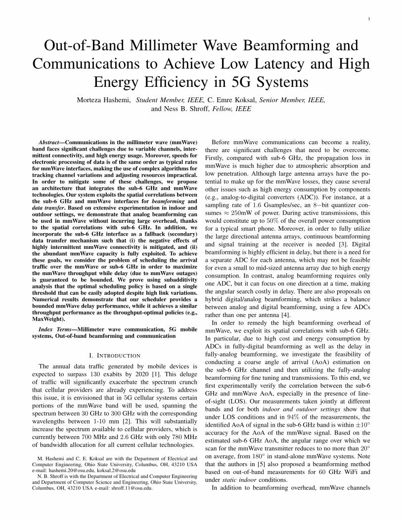
Fig. 1. Our integrated sub-6 GHz–mmWave architecture where the speed of mmWave interface necessitates the use of a separate queue.
across different interfaces under various conditions, includingindoor and outdoor situations, with mobility, and LOS.
In order to improve mmWave beamforming efficiency, therehas been extensive amount of work on digital and analogbeamforming (e.g., [3, 12]). There are also proposals on hybridbeamforming methods [4] in which the term “hybrid” refers tothe mixture of analog/digital (different from our hybrid sub-6GHz/mmWave system). The whole operation there is in solemmWave domain. The authors in [13] propose a compressedbeamforming method that is based on out-of-band spatialinformation obtained at the sub-6 GHz band. In this paper,we experimentally investigate the sub-6 GHz/mmWave spatialcorrelations under practical (e.g., with mobility) scenarios, anddemonstrate that how mobility affects the channel conditionsand cross-interface correlation.
(II) Out-of-Band communications and scheduling poli-cies: In the second part of this paper, we use sub-6 GHzas an auxiliary data transfer interface. Similar to our model,the authors in [14] studied a dual-interface system to offloadcellular data over WiFi network. In this work, the delay and ef-ficiency are quantified in a simple interface selection strategy,where the WiFi interface is selected whenever it is availableand the cellular interface is selected when a specified deadline,Tout, is expired for buffered packets. In order to enable dual-interface communications and data transfer using sub-6 GHzand mmWave, we include a load division component in ourproposed architecture (see Fig. 1). The objective is to schedulethe arrival traffic over the sub-6 GHz or mmWave interfacesuch that the maximum mmWave throughput with a boundeddelay performance is achieved.
In the context of wireless scheduling policies, backpres-sure algorithms [15] promise throughput-optimal performance,which leads to a problem, known as MaxWeight. Using thisframework, the goal is to maximize the weighted sum oflink rates, in which the weights are represented by backlogdifferences of queues. Although backpressure-type algorithmsprovide throughput-optimal performance, they suffer fromhigh end-to-end delays. To mitigate this issue, several ap-proaches have been proposed. For instance, [16] proposesbackpressure with adaptive redundancy (BWAR) to improvethe delay performance. [17] describes a backpressure-basedper-packet randomized routing framework to improve thedelay performance. The authors in [18] propose using delayinformation of packets in the queues instead of using queuedifferentials as weights of the MaxWeight problem. As a result,those packets that have experienced high delays are more
likely to be scheduled in the next time slot.Due to the high data rate of the mmWave interface, it may
not be feasible to track the channel state in real-time. Thismakes the use of complex algorithms to track the channel vari-ations impractical. In this paper, we devise a delay-constrainedand throughput-optimal scheduling policy that is expressed interms of the queue lengths. To the best of our knowledge,there is no previous work that considers an integrated sub-6GHz/mmWave architecture for beamforming and optimal datascheduling across the sub-6 GHz and mmWave interfaces.
III. INTEGRATED SUB-6 GHZ – MMWAVE ARCHITECTURE
A. System Model
Figure 1 illustrates the basic components of our architec-ture. The proposed architecture exploits the cross-interfacecorrelation to achieve the beamforming fully in the analogdomain without incurring high delay overhead. Thus, the ADCfollows the beamformer at the receiver, and eliminates the needfor a separate one, for all elements in the mmWave antenna-array. In addition, we move all mmWave control signaling andchannel state information (CSI) feedback to the sub-6 GHzinterface, and thus we avoid the two-way beamforming andreverse channel transmission costs in mmWave.
In addition to high energy consumption by components, themmWave channel is highly sensitive and outages can be longthat can lead to unacceptably high delays for delay-sensitiveapplications. However, a conservative use of the mmWavelink is not desirable either, since the upside of the mmWavechannel can be enormous, especially in the presence of LOSthat occurs intermittently. More importantly, the high data rateof the mmWave link necessitates the use of a reasonably largebuffer at the mmWave interface along with proactive queue-control solutions. Therefore, we consider a load devisioncomponent in Fig. 1 along with the separate sub-6 GHz andmmWave queues. We derive an optimal scheduling policy toselect which interface(s) to use and control the queue sizes ofinterfaces in order to achieve maximum mmWave throughputwith constrained delay. We investigate the optimal interfacescheduling in Section IV.
B. Sub-6 GHz System and Channel Model
For the sub-6 GHz system, we use digital beamforming asshown in Fig. 2. As a result, the received signal at the receivercan be written as:
ysub-6 = Hsub-6 · xsub-6 + nsub-6, (1)
RF ChainDAC
DAC RF Chain
Ba
seb
and
Ba
seb
and
ADCRF Chain
ADCRF Chain
Hsub-6
Transmitter Receiver
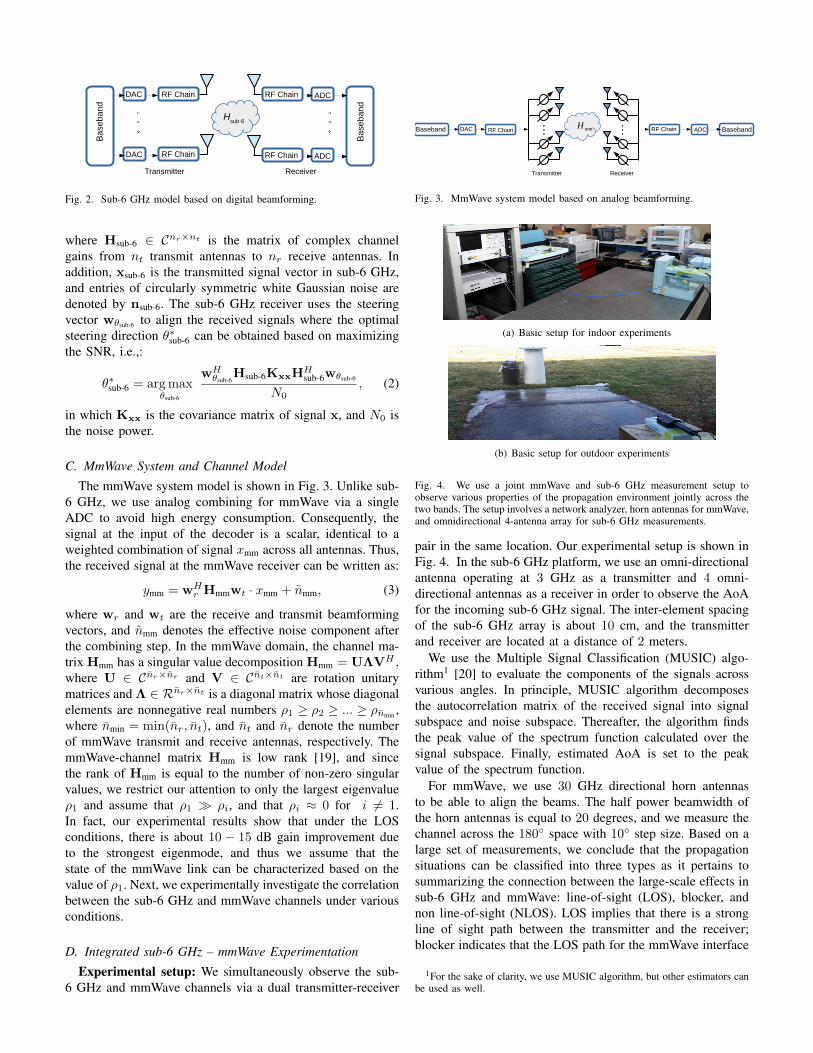
Fig. 2. Sub-6 GHz model based on digital beamforming.
where Hsub-6 ∈ Cnr×nt is the matrix of complex channelgains from nt transmit antennas to nr receive antennas. Inaddition, xsub-6 is the transmitted signal vector in sub-6 GHz,and entries of circularly symmetric white Gaussian noise aredenoted by nsub-6. The sub-6 GHz receiver uses the steeringvector wθsub-6 to align the received signals where the optimalsteering direction θ∗sub-6 can be obtained based on maximizingthe SNR, i.e.,:
θ∗sub-6 = arg maxθsub-6
wHθsub-6
Hsub-6KxxHHsub-6wθsub-6
N0, (2)
in which Kxx is the covariance matrix of signal x, and N0 isthe noise power.
C. MmWave System and Channel Model
The mmWave system model is shown in Fig. 3. Unlike sub-6 GHz, we use analog combining for mmWave via a singleADC to avoid high energy consumption. Consequently, thesignal at the input of the decoder is a scalar, identical to aweighted combination of signal xmm across all antennas. Thus,the received signal at the mmWave receiver can be written as:
ymm = wHr Hmmwt · xmm + nmm, (3)
where wr and wt are the receive and transmit beamformingvectors, and nmm denotes the effective noise component afterthe combining step. In the mmWave domain, the channel ma-trix Hmm has a singular value decomposition Hmm = UΛVH ,where U ∈ Cnr×nr and V ∈ Cnt×nt are rotation unitarymatrices and Λ ∈ Rnr×nt is a diagonal matrix whose diagonalelements are nonnegative real numbers ρ1 ≥ ρ2 ≥ ... ≥ ρnmin ,where nmin = min(nr, nt), and nt and nr denote the numberof mmWave transmit and receive antennas, respectively. ThemmWave-channel matrix Hmm is low rank [19], and sincethe rank of Hmm is equal to the number of non-zero singularvalues, we restrict our attention to only the largest eigenvalueρ1 and assume that ρ1 � ρi, and that ρi ≈ 0 for i 6= 1.In fact, our experimental results show that under the LOSconditions, there is about 10 − 15 dB gain improvement dueto the strongest eigenmode, and thus we assume that thestate of the mmWave link can be characterized based on thevalue of ρ1. Next, we experimentally investigate the correlationbetween the sub-6 GHz and mmWave channels under variousconditions.
D. Integrated sub-6 GHz – mmWave Experimentation
Experimental setup: We simultaneously observe the sub-6 GHz and mmWave channels via a dual transmitter-receiver
RF ChainDACBaseband Hmm RF Chain ADC Baseband
Transmitter Receiver
Fig. 3. MmWave system model based on analog beamforming.
(a) Basic setup for indoor experiments
(b) Basic setup for outdoor experiments
Fig. 4. We use a joint mmWave and sub-6 GHz measurement setup toobserve various properties of the propagation environment jointly across thetwo bands. The setup involves a network analyzer, horn antennas for mmWave,and omnidirectional 4-antenna array for sub-6 GHz measurements.
pair in the same location. Our experimental setup is shown inFig. 4. In the sub-6 GHz platform, we use an omni-directionalantenna operating at 3 GHz as a transmitter and 4 omni-directional antennas as a receiver in order to observe the AoAfor the incoming sub-6 GHz signal. The inter-element spacingof the sub-6 GHz array is about 10 cm, and the transmitterand receiver are located at a distance of 2 meters.
We use the Multiple Signal Classification (MUSIC) algo-rithm1 [20] to evaluate the components of the signals acrossvarious angles. In principle, MUSIC algorithm decomposesthe autocorrelation matrix of the received signal into signalsubspace and noise subspace. Thereafter, the algorithm findsthe peak value of the spectrum function calculated over thesignal subspace. Finally, estimated AoA is set to the peakvalue of the spectrum function.
For mmWave, we use 30 GHz directional horn antennasto be able to align the beams. The half power beamwidth ofthe horn antennas is equal to 20 degrees, and we measure thechannel across the 180◦ space with 10◦ step size. Based on alarge set of measurements, we conclude that the propagationsituations can be classified into three types as it pertains tosummarizing the connection between the large-scale effects insub-6 GHz and mmWave: line-of-sight (LOS), blocker, andnon line-of-sight (NLOS). LOS implies that there is a strongline of sight path between the transmitter and the receiver;blocker indicates that the LOS path for the mmWave interface
1For the sake of clarity, we use MUSIC algorithm, but other estimators canbe used as well.
0 20 40 60 80 100 120 140 160 180angle of observation
0.2
0.3
0.4
0.5
0.6
0.7
MU
SIC
outp
ut (s
ub-6
GH
z)
LOS
blocker
reflection
0 20 40 60 80 100 120 140 160 180
angle of observation
0
0.2
0.4
0.6
0.8
1
1.2
Sig
nal S
trength
(m
mW
ave)
10-4
LOS
blocker
reflection
(a) sub-6 GHz and mmWave activity vs. angle in indoor setting
0 20 40 60 80 100 120 140 160 180
angle of observation
0.2
0.4
0.6
0.8
1
1.2
MU
SIC
outp
ut (s
ub-6
GH
z)
LOS
blocker
reflection
0 20 40 60 80 100 120 140 160 180
angle of observation
0
0.5
1
1.5
2
Sig
nal S
trength
(m
mW
ave)
10-4
LOS
blocker
reflection
(b) sub-6 GHz and mmWave activity vs. angle in outdoor setting
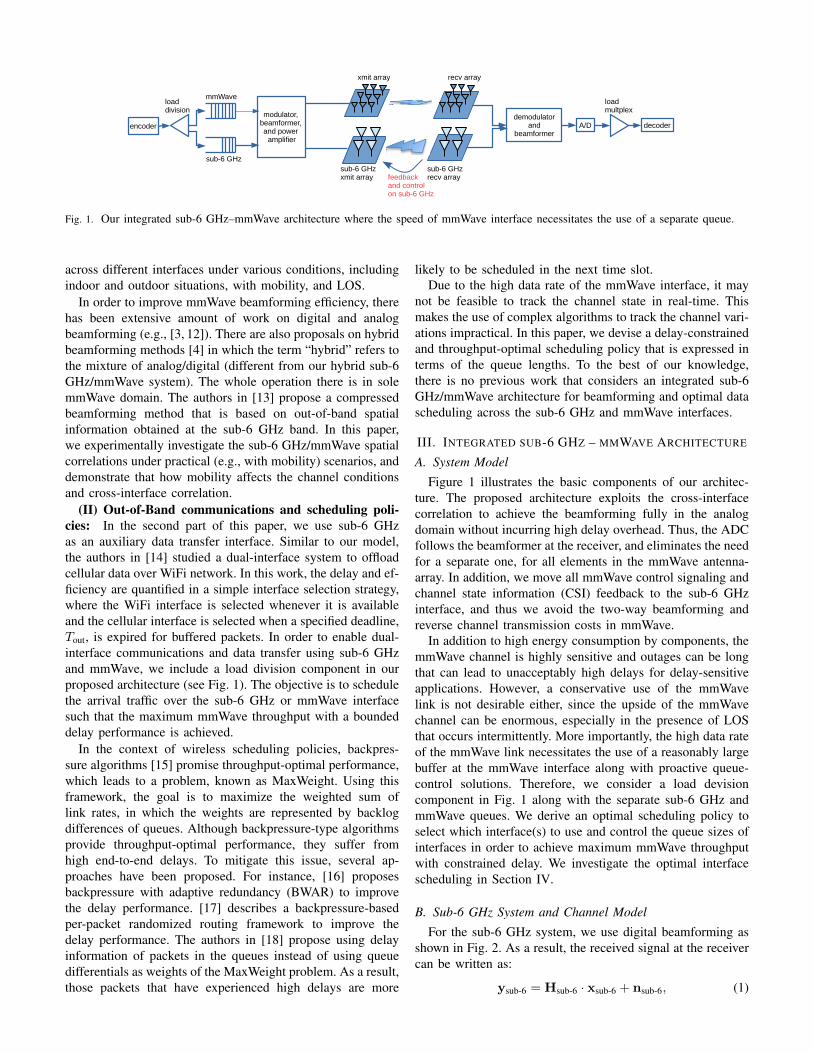
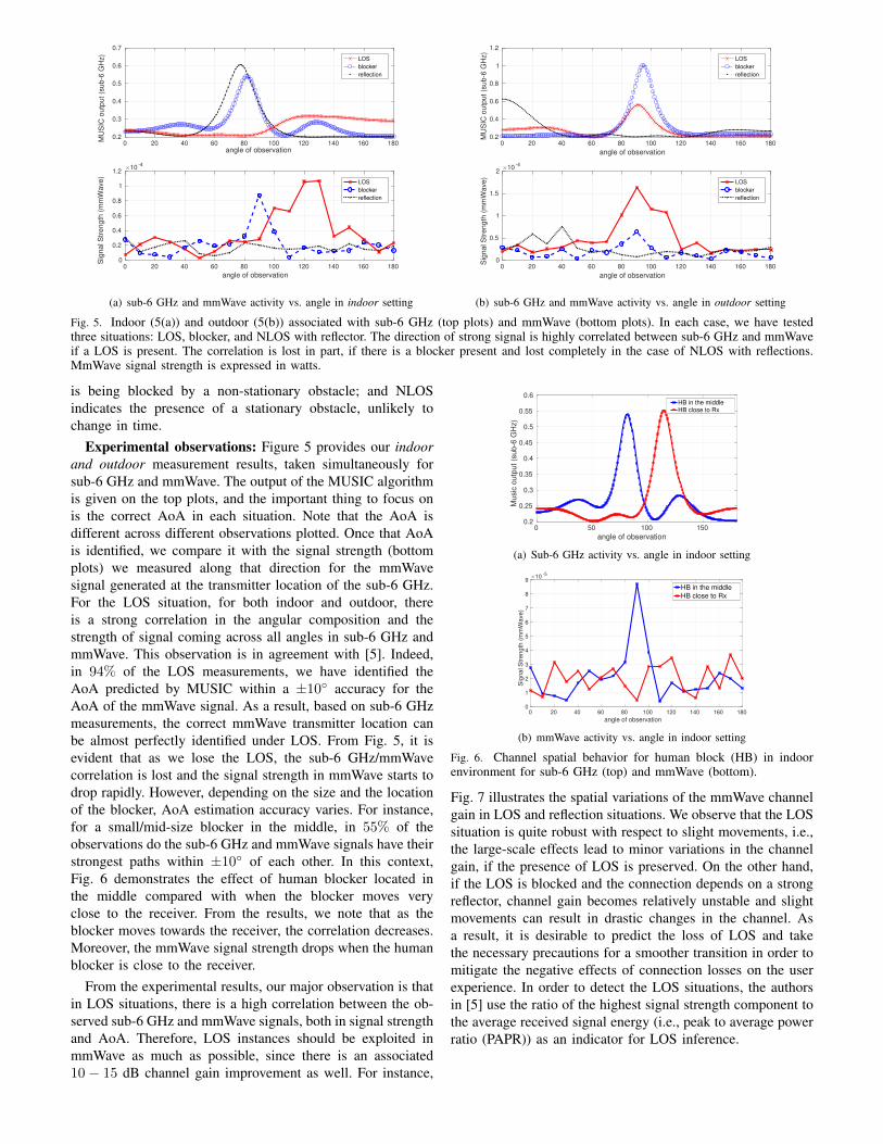
Fig. 5. Indoor (5(a)) and outdoor (5(b)) associated with sub-6 GHz (top plots) and mmWave (bottom plots). In each case, we have testedthree situations: LOS, blocker, and NLOS with reflector. The direction of strong signal is highly correlated between sub-6 GHz and mmWaveif a LOS is present. The correlation is lost in part, if there is a blocker present and lost completely in the case of NLOS with reflections.MmWave signal strength is expressed in watts.
is being blocked by a non-stationary obstacle; and NLOSindicates the presence of a stationary obstacle, unlikely tochange in time.
Experimental observations: Figure 5 provides our indoorand outdoor measurement results, taken simultaneously forsub-6 GHz and mmWave. The output of the MUSIC algorithmis given on the top plots, and the important thing to focus onis the correct AoA in each situation. Note that the AoA isdifferent across different observations plotted. Once that AoAis identified, we compare it with the signal strength (bottomplots) we measured along that direction for the mmWavesignal generated at the transmitter location of the sub-6 GHz.For the LOS situation, for both indoor and outdoor, thereis a strong correlation in the angular composition and thestrength of signal coming across all angles in sub-6 GHz andmmWave. This observation is in agreement with [5]. Indeed,in 94% of the LOS measurements, we have identified theAoA predicted by MUSIC within a ±10◦ accuracy for theAoA of the mmWave signal. As a result, based on sub-6 GHzmeasurements, the correct mmWave transmitter location canbe almost perfectly identified under LOS. From Fig. 5, it isevident that as we lose the LOS, the sub-6 GHz/mmWavecorrelation is lost and the signal strength in mmWave starts todrop rapidly. However, depending on the size and the locationof the blocker, AoA estimation accuracy varies. For instance,for a small/mid-size blocker in the middle, in 55% of theobservations do the sub-6 GHz and mmWave signals have theirstrongest paths within ±10◦ of each other. In this context,Fig. 6 demonstrates the effect of human blocker located inthe middle compared with when the blocker moves veryclose to the receiver. From the results, we note that as theblocker moves towards the receiver, the correlation decreases.Moreover, the mmWave signal strength drops when the humanblocker is close to the receiver.
From the experimental results, our major observation is thatin LOS situations, there is a high correlation between the ob-served sub-6 GHz and mmWave signals, both in signal strengthand AoA. Therefore, LOS instances should be exploited inmmWave as much as possible, since there is an associated10 − 15 dB channel gain improvement as well. For instance,
0 50 100 150
angle of observation
0.2
0.25
0.3
0.35
0.4
0.45
0.5
0.55
0.6
Music
outp
ut (s
ub-6
GH
z)
HB in the middleHB close to Rx
(a) Sub-6 GHz activity vs. angle in indoor setting
0 20 40 60 80 100 120 140 160 180
angle of observation
0
1
2
3
4
5
6
7
8
9
Sig
na
l S
tre
ng
th (
mm
Wa
ve
)
10-5
HB in the middle
HB close to Rx
(b) mmWave activity vs. angle in indoor setting
Fig. 6. Channel spatial behavior for human block (HB) in indoorenvironment for sub-6 GHz (top) and mmWave (bottom).
Fig. 7 illustrates the spatial variations of the mmWave channelgain in LOS and reflection situations. We observe that the LOSsituation is quite robust with respect to slight movements, i.e.,the large-scale effects lead to minor variations in the channelgain, if the presence of LOS is preserved. On the other hand,if the LOS is blocked and the connection depends on a strongreflector, channel gain becomes relatively unstable and slightmovements can result in drastic changes in the channel. Asa result, it is desirable to predict the loss of LOS and takethe necessary precautions for a smoother transition in order tomitigate the negative effects of connection losses on the userexperience. In order to detect the LOS situations, the authorsin [5] use the ratio of the highest signal strength component tothe average received signal energy (i.e., peak to average powerratio (PAPR)) as an indicator for LOS inference.
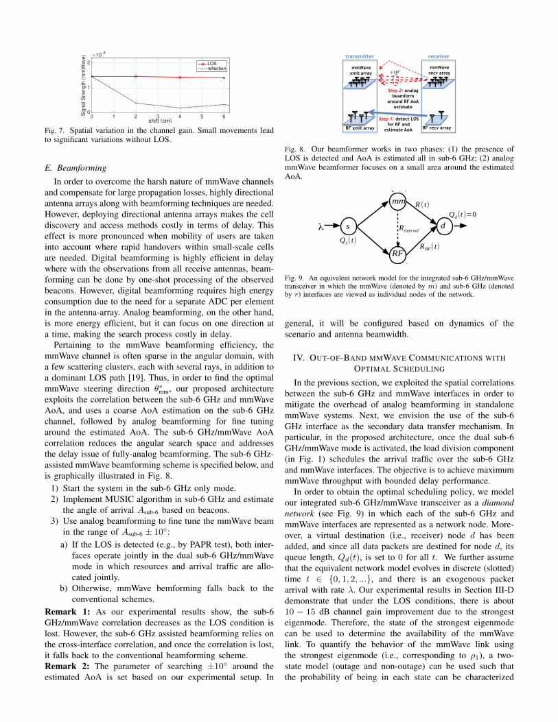
shift (cm)0 1 2 3 4 5 6S
ignal S
trength
(m
mW
ave) ×10
-4
0
1
2 LOSreflection
Fig. 7. Spatial variation in the channel gain. Small movements leadto significant variations without LOS.
E. Beamforming
In order to overcome the harsh nature of mmWave channelsand compensate for large propagation losses, highly directionalantenna arrays along with beamforming techniques are needed.However, deploying directional antenna arrays makes the celldiscovery and access methods costly in terms of delay. Thiseffect is more pronounced when mobility of users are takeninto account where rapid handovers within small-scale cellsare needed. Digital beamforming is highly efficient in delaywhere with the observations from all receive antennas, beam-forming can be done by one-shot processing of the observedbeacons. However, digital beamforming requires high energyconsumption due to the need for a separate ADC per elementin the antenna-array. Analog beamforming, on the other hand,is more energy efficient, but it can focus on one direction ata time, making the search process costly in delay.
Pertaining to the mmWave beamforming efficiency, themmWave channel is often sparse in the angular domain, witha few scattering clusters, each with several rays, in addition toa dominant LOS path [19]. Thus, in order to find the optimalmmWave steering direction θ∗mm, our proposed architectureexploits the correlation between the sub-6 GHz and mmWaveAoA, and uses a coarse AoA estimation on the sub-6 GHzchannel, followed by analog beamforming for fine tuningaround the estimated AoA. The sub-6 GHz/mmWave AoAcorrelation reduces the angular search space and addressesthe delay issue of fully-analog beamforming. The sub-6 GHz-assisted mmWave beamforming scheme is specified below, andis graphically illustrated in Fig. 8.
1) Start the system in the sub-6 GHz only mode.2) Implement MUSIC algorithm in sub-6 GHz and estimate
the angle of arrival Asub-6 based on beacons.3) Use analog beamforming to fine tune the mmWave beam
in the range of Asub-6 ± 10◦:a) If the LOS is detected (e.g., by PAPR test), both inter-
faces operate jointly in the dual sub-6 GHz/mmWavemode in which resources and arrival traffic are allo-cated jointly.
b) Otherwise, mmWave bemforming falls back to theconventional schemes.
Remark 1: As our experimental results show, the sub-6GHz/mmWave correlation decreases as the LOS condition islost. However, the sub-6 GHz assisted beamforming relies onthe cross-interface correlation, and once the correlation is lost,it falls back to the conventional beamforming scheme.Remark 2: The parameter of searching ±10◦ around theestimated AoA is set based on our experimental setup. In
mmWave xmit array
mmWave recv array
RF recv array
Step 1: detect LOS for RF and
estimate AoA
Step 2: analog beamform
around RF AoA estimate
⌥10�
RF xmit array
transmitter receiver
Fig. 8. Our beamformer works in two phases: (1) the presence ofLOS is detected and AoA is estimated all in sub-6 GHz; (2) analogmmWave beamformer focuses on a small area around the estimatedAoA.
Fig. 9. An equivalent network model for the integrated sub-6 GHz/mmWavetransceiver in which the mmWave (denoted by m) and sub-6 GHz (denotedby r) interfaces are viewed as individual nodes of the network.
general, it will be configured based on dynamics of thescenario and antenna beamwidth.
IV. OUT-OF-BAND MMWAVE COMMUNICATIONS WITHOPTIMAL SCHEDULING
In the previous section, we exploited the spatial correlationsbetween the sub-6 GHz and mmWave interfaces in order tomitigate the overhead of analog beamforming in standalonemmWave systems. Next, we envision the use of the sub-6GHz interface as the secondary data transfer mechanism. Inparticular, in the proposed architecture, once the dual sub-6GHz/mmWave mode is activated, the load division component(in Fig. 1) schedules the arrival traffic over the sub-6 GHzand mmWave interfaces. The objective is to achieve maximummmWave throughput with bounded delay performance.
In order to obtain the optimal scheduling policy, we modelour integrated sub-6 GHz/mmWave transceiver as a diamondnetwork (see Fig. 9) in which each of the sub-6 GHz andmmWave interfaces are represented as a network node. More-over, a virtual destination (i.e., receiver) node d has beenadded, and since all data packets are destined for node d, itsqueue length, Qd(t), is set to 0 for all t. We further assumethat the equivalent network model evolves in discrete (slotted)time t ∈ {0, 1, 2, ...}, and there is an exogenous packetarrival with rate λ. Our experimental results in Section III-Ddemonstrate that under the LOS conditions, there is about10 − 15 dB channel gain improvement due to the strongesteigenmode. Therefore, the state of the strongest eigenmodecan be used to determine the availability of the mmWavelink. To quantify the behavior of the mmWave link usingthe strongest eigenmode (i.e., corresponding to ρ1), a two-state model (outage and non-outage) can be used such thatthe probability of being in each state can be characterized
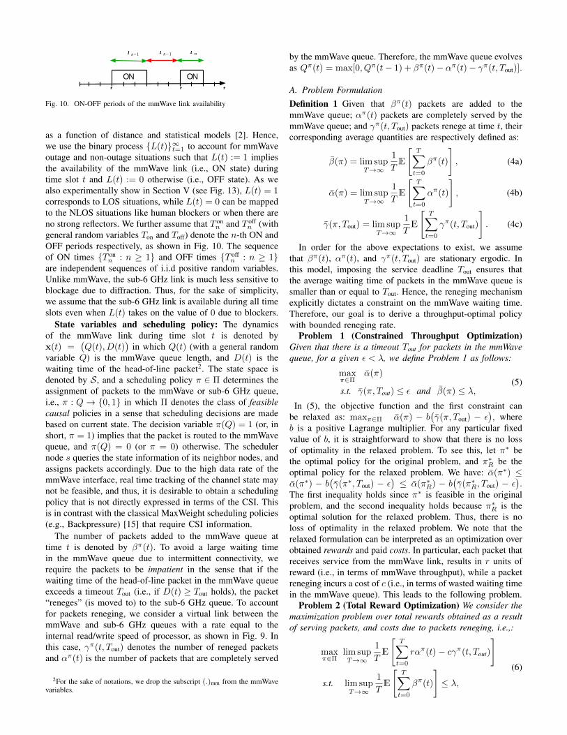
Fig. 10. ON-OFF periods of the mmWave link availability
as a function of distance and statistical models [2]. Hence,we use the binary process {L(t)}∞t=1 to account for mmWaveoutage and non-outage situations such that L(t) := 1 impliesthe availability of the mmWave link (i.e., ON state) duringtime slot t and L(t) := 0 otherwise (i.e., OFF state). As wealso experimentally show in Section V (see Fig. 13), L(t) = 1corresponds to LOS situations, while L(t) = 0 can be mappedto the NLOS situations like human blockers or when there areno strong reflectors. We further assume that T on
n and T offn (with
general random variables Ton and Toff) denote the n-th ON andOFF periods respectively, as shown in Fig. 10. The sequenceof ON times {T on
n : n ≥ 1} and OFF times {T offn : n ≥ 1}
are independent sequences of i.i.d positive random variables.Unlike mmWave, the sub-6 GHz link is much less sensitive toblockage due to diffraction. Thus, for the sake of simplicity,we assume that the sub-6 GHz link is available during all timeslots even when L(t) takes on the value of 0 due to blockers.
State variables and scheduling policy: The dynamicsof the mmWave link during time slot t is denoted byx(t) =
(Q(t), D(t)
)in which Q(t) (with a general random
variable Q) is the mmWave queue length, and D(t) is thewaiting time of the head-of-line packet2. The state space isdenoted by S, and a scheduling policy π ∈ Π determines theassignment of packets to the mmWave or sub-6 GHz queue,i.e., π : Q → {0, 1} in which Π denotes the class of feasiblecausal policies in a sense that scheduling decisions are madebased on current state. The decision variable π(Q) = 1 (or, inshort, π = 1) implies that the packet is routed to the mmWavequeue, and π(Q) = 0 (or π = 0) otherwise. The schedulernode s queries the state information of its neighbor nodes, andassigns packets accordingly. Due to the high data rate of themmWave interface, real time tracking of the channel state maynot be feasible, and thus, it is desirable to obtain a schedulingpolicy that is not directly expressed in terms of the CSI. Thisis in contrast with the classical MaxWeight scheduling policies(e.g., Backpressure) [15] that require CSI information.
The number of packets added to the mmWave queue attime t is denoted by βπ(t). To avoid a large waiting timein the mmWave queue due to intermittent connectivity, werequire the packets to be impatient in the sense that if thewaiting time of the head-of-line packet in the mmWave queueexceeds a timeout Tout (i.e., if D(t) ≥ Tout holds), the packet“reneges” (is moved to) to the sub-6 GHz queue. To accountfor packets reneging, we consider a virtual link between themmWave and sub-6 GHz queues with a rate equal to theinternal read/write speed of processor, as shown in Fig. 9. Inthis case, γπ(t, Tout) denotes the number of reneged packetsand απ(t) is the number of packets that are completely served
2For the sake of notations, we drop the subscript (.)mm from the mmWavevariables.
by the mmWave queue. Therefore, the mmWave queue evolvesas Qπ(t) = max[0, Qπ(t− 1) + βπ(t)− απ(t)− γπ(t, Tout)].
A. Problem FormulationDefinition 1 Given that βπ(t) packets are added to themmWave queue; απ(t) packets are completely served by themmWave queue; and γπ(t, Tout) packets renege at time t, theircorresponding average quantities are respectively defined as:
β(π) = lim supT→∞
1
TE
[T∑t=0
βπ(t)
], (4a)
α(π) = lim supT→∞
1
TE
[T∑t=0
απ(t)
], (4b)
γ(π, Tout) = lim supT→∞
1
TE
[T∑t=0
γπ(t, Tout)
]. (4c)
In order for the above expectations to exist, we assumethat βπ(t), απ(t), and γπ(t, Tout) are stationary ergodic. Inthis model, imposing the service deadline Tout ensures thatthe average waiting time of packets in the mmWave queue issmaller than or equal to Tout. Hence, the reneging mechanismexplicitly dictates a constraint on the mmWave waiting time.Therefore, our goal is to derive a throughput-optimal policywith bounded reneging rate.
Problem 1 (Constrained Throughput Optimization)Given that there is a timeout Tout for packets in the mmWavequeue, for a given ε < λ, we define Problem 1 as follows:
maxπ∈Π
α(π)
s.t. γ(π, Tout) ≤ ε and β(π) ≤ λ,(5)
In (5), the objective function and the first constraint canbe relaxed as: maxπ∈Π α(π) − b
(γ(π, Tout) − ε
), where
b is a positive Lagrange multiplier. For any particular fixedvalue of b, it is straightforward to show that there is no lossof optimality in the relaxed problem. To see this, let π∗ bethe optimal policy for the original problem, and π∗R be theoptimal policy for the relaxed problem. We have: α(π∗) ≤α(π∗) − b
(γ(π∗, Tout) − ε
)≤ α(π∗R) − b
(γ(π∗R, Tout) − ε
).
The first inequality holds since π∗ is feasible in the originalproblem, and the second inequality holds because π∗R is theoptimal solution for the relaxed problem. Thus, there is noloss of optimality in the relaxed problem. We note that therelaxed formulation can be interpreted as an optimization overobtained rewards and paid costs. In particular, each packet thatreceives service from the mmWave link, results in r units ofreward (i.e., in terms of mmWave throughput), while a packetreneging incurs a cost of c (i.e., in terms of wasted waiting timein the mmWave queue). This leads to the following problem.
Problem 2 (Total Reward Optimization) We consider themaximization problem over total rewards obtained as a resultof serving packets, and costs due to packets reneging, i.e.,:
maxπ∈Π
lim supT→∞
1
TE
[T∑t=0
rαπ(t)− cγπ(t, Tout)
]
s.t. lim supT→∞
1
TE
[T∑t=0
βπ(t)
]≤ λ,
(6)
0 0.2 0.4 0.6 0.8 1Admission probability
-1
-0.5
0
0.5
1
Ave
rag
e r
ew
ard
104
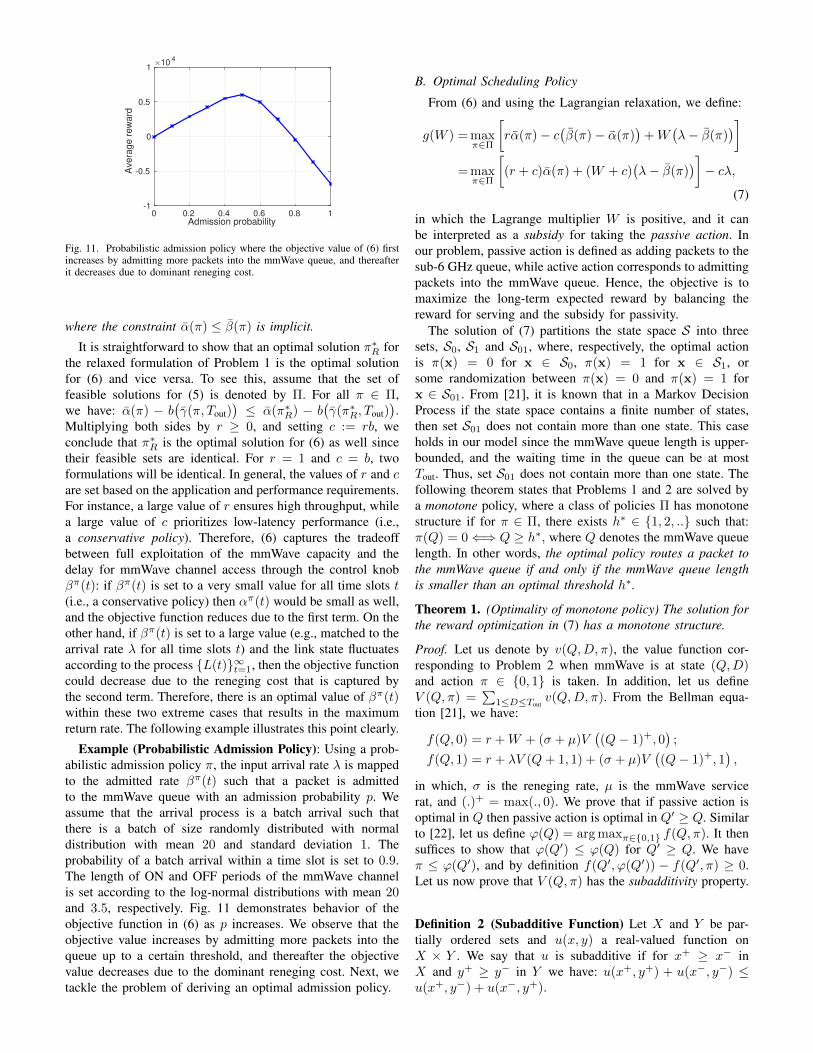
Fig. 11. Probabilistic admission policy where the objective value of (6) firstincreases by admitting more packets into the mmWave queue, and thereafterit decreases due to dominant reneging cost.
where the constraint α(π) ≤ β(π) is implicit.
It is straightforward to show that an optimal solution π∗R forthe relaxed formulation of Problem 1 is the optimal solutionfor (6) and vice versa. To see this, assume that the set offeasible solutions for (5) is denoted by Π. For all π ∈ Π,we have: α(π) − b
(γ(π, Tout)
)≤ α(π∗R) − b
(γ(π∗R, Tout)
).
Multiplying both sides by r ≥ 0, and setting c := rb, weconclude that π∗R is the optimal solution for (6) as well sincetheir feasible sets are identical. For r = 1 and c = b, twoformulations will be identical. In general, the values of r and care set based on the application and performance requirements.For instance, a large value of r ensures high throughput, whilea large value of c prioritizes low-latency performance (i.e.,a conservative policy). Therefore, (6) captures the tradeoffbetween full exploitation of the mmWave capacity and thedelay for mmWave channel access through the control knobβπ(t): if βπ(t) is set to a very small value for all time slots t(i.e., a conservative policy) then απ(t) would be small as well,and the objective function reduces due to the first term. On theother hand, if βπ(t) is set to a large value (e.g., matched to thearrival rate λ for all time slots t) and the link state fluctuatesaccording to the process {L(t)}∞t=1, then the objective functioncould decrease due to the reneging cost that is captured bythe second term. Therefore, there is an optimal value of βπ(t)within these two extreme cases that results in the maximumreturn rate. The following example illustrates this point clearly.
Example (Probabilistic Admission Policy): Using a prob-abilistic admission policy π, the input arrival rate λ is mappedto the admitted rate βπ(t) such that a packet is admittedto the mmWave queue with an admission probability p. Weassume that the arrival process is a batch arrival such thatthere is a batch of size randomly distributed with normaldistribution with mean 20 and standard deviation 1. Theprobability of a batch arrival within a time slot is set to 0.9.The length of ON and OFF periods of the mmWave channelis set according to the log-normal distributions with mean 20and 3.5, respectively. Fig. 11 demonstrates behavior of theobjective function in (6) as p increases. We observe that theobjective value increases by admitting more packets into thequeue up to a certain threshold, and thereafter the objectivevalue decreases due to the dominant reneging cost. Next, wetackle the problem of deriving an optimal admission policy.
B. Optimal Scheduling Policy
From (6) and using the Lagrangian relaxation, we define:
g(W ) = maxπ∈Π
[rα(π)− c
(β(π)− α(π)
)+W
(λ− β(π)
)]= max
π∈Π
[(r + c)α(π) + (W + c)
(λ− β(π)
)]− cλ,
(7)
in which the Lagrange multiplier W is positive, and it canbe interpreted as a subsidy for taking the passive action. Inour problem, passive action is defined as adding packets to thesub-6 GHz queue, while active action corresponds to admittingpackets into the mmWave queue. Hence, the objective is tomaximize the long-term expected reward by balancing thereward for serving and the subsidy for passivity.
The solution of (7) partitions the state space S into threesets, S0, S1 and S01, where, respectively, the optimal actionis π(x) = 0 for x ∈ S0, π(x) = 1 for x ∈ S1, orsome randomization between π(x) = 0 and π(x) = 1 forx ∈ S01. From [21], it is known that in a Markov DecisionProcess if the state space contains a finite number of states,then set S01 does not contain more than one state. This caseholds in our model since the mmWave queue length is upper-bounded, and the waiting time in the queue can be at mostTout. Thus, set S01 does not contain more than one state. Thefollowing theorem states that Problems 1 and 2 are solved bya monotone policy, where a class of policies Π has monotonestructure if for π ∈ Π, there exists h∗ ∈ {1, 2, ..} such that:π(Q) = 0⇐⇒ Q ≥ h∗, where Q denotes the mmWave queuelength. In other words, the optimal policy routes a packet tothe mmWave queue if and only if the mmWave queue lengthis smaller than an optimal threshold h∗.
Theorem 1. (Optimality of monotone policy) The solution forthe reward optimization in (7) has a monotone structure.
Proof. Let us denote by v(Q,D, π), the value function cor-responding to Problem 2 when mmWave is at state (Q,D)and action π ∈ {0, 1} is taken. In addition, let us defineV (Q, π) =
∑1≤D≤Tout
v(Q,D, π). From the Bellman equa-tion [21], we have:
f(Q, 0) = r +W + (σ + µ)V((Q− 1)+, 0
);
f(Q, 1) = r + λV (Q+ 1, 1) + (σ + µ)V((Q− 1)+, 1
),
in which, σ is the reneging rate, µ is the mmWave servicerat, and (.)+ = max(., 0). We prove that if passive action isoptimal in Q then passive action is optimal in Q′ ≥ Q. Similarto [22], let us define ϕ(Q) = arg maxπ∈{0,1} f(Q, π). It thensuffices to show that ϕ(Q′) ≤ ϕ(Q) for Q′ ≥ Q. We haveπ ≤ ϕ(Q′), and by definition f(Q′, ϕ(Q′)) − f(Q′, π) ≥ 0.Let us now prove that V (Q, π) has the subadditivity property.
Definition 2 (Subadditive Function) Let X and Y be par-tially ordered sets and u(x, y) a real-valued function onX × Y . We say that u is subadditive if for x+ ≥ x− inX and y+ ≥ y− in Y we have: u(x+, y+) + u(x−, y−) ≤u(x+, y−) + u(x−, y+).
To prove that V (Q, π) is a subadditive function, it sufficesto show that for all Q′ ≥ Q and π ∈ {0, 1}, the inequalityf(Q′, ϕ(Q′)) + f(Q, π) ≤ f(Q′, π) + f(Q,ϕ(Q′)) holds. Ifϕ(Q′) = π = 0 or ϕ(Q′) = π = 1, then the inequalityis satisfied. If ϕ(Q′) = 1 and π = 0, then we show thatf(Q, 0) − f(Q, 1) ≤ f(Q, 1) − f(Q′, 1). By replacing thecorresponding terms, we need to show:
(σ + µ)[V((Q− 1)+, 0
)− V
((Q′ − 1)+, 0
)]≤
λ [V (Q+ 1, 1)− V (Q′ + 1, 1)]
+(σ + µ)[V((Q− 1)+, 1
)− V
((Q′ − 1)+, 1
)]. (8)
In order to show this inequality, we note that V (Q, 1) isnon-increasing and V (Q, 0) is non-decreasing. The reasonis that when the action π = 1 is chosen, all packets willbe added to the mmWave queue. The likelihood that anadmitted packet reneges before receiving service increaseswith the number of queued packets, and thus the incurredreneging cost increases. Therefore, the value function V (Q, 1)is a non-increasing function of the queue length. A sim-ilar argument holds for V (Q, 0). Therefore, the inequalityf(Q, 0)−f(Q, 1) ≤ f(Q, 1)−f(Q′, 1) holds, and the theoremstatement follows.
Intuitively, for a first-in-first-out (FIFO) queue, the likeli-hood that an admitted packet reneges before receiving serviceincreases with the number of queued packets. Therefore, giventhat the reneging and moving packets from the mmWave queueto the sub-6 GHz queue incurs a delay cost, it is in thescheduler interest to exercise admission control and deny entryto packets when the mmWave queue grows and becomes largerthan a threshold. Next, we characterize the optimal threshold.
C. Optimal Threshold
Optimal policy π∗ imposes a threshold h∗ ∈ {0, 1, 2, ..}such that π∗(Q) = 1 if and only if Q < h∗. Under theergodicity assumption, we rewrite Problem 2 as:
maxh∈{0,1,2,..}
((r + c
)E[αh]−
(W + c
)E[βh]
). (9)
Lemma 1. Given an admission threshold h, if
ψ(h) :=E[βh]− E[βh−1]
E[αh]− E[αh−1], (10)
then ψ(h) is non-decreasing in h.
Proof. In order to prove that ψ(h) is non-decreasing, we notethat both E[αh] and E[βh] are non-decreasing in h sincea larger threshold h results in admitting more packets (i.e.,a larger E[βh]) and potentially a higher throughput E[αh].Moreover, E[βh] is assumed to be an affine function of h. Inorder to prove that ψ(h) is non-decreasing in h, we need toshow that ψ(h+1)−ψ(h) ≥ 0 for h ≥ 0. Therefore, we have:
ψ(h+ 1)− ψ(h) =(E[αh]− E[αh−1]) (E[βh+1]− E[βh])
(E[αh+1]− E[αh]) (E[αh]− E[αh−1])
− (E[βh]− E[βh−1]) (E[αh+1]− E[αh])
(E[αh+1]− E[αh]) (E[αh]− E[αh−1])
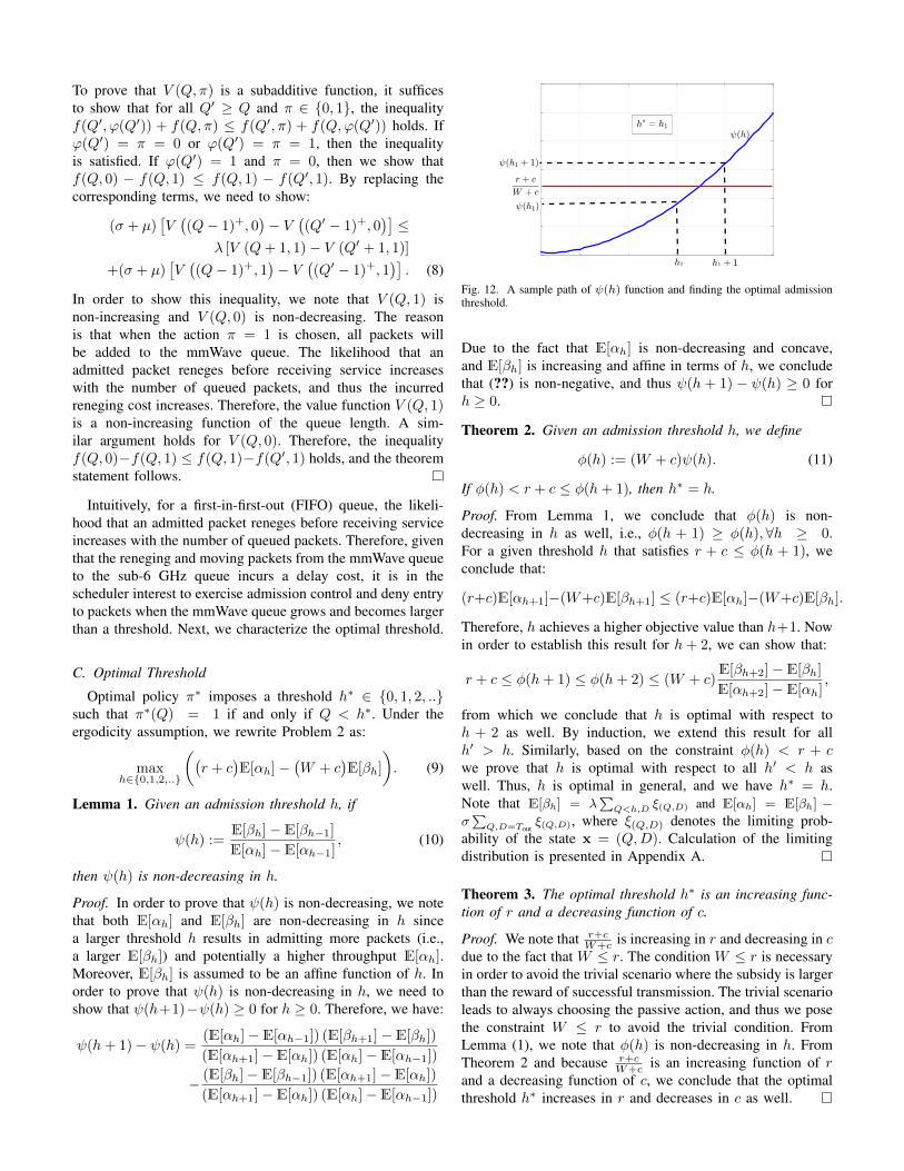
Fig. 12. A sample path of ψ(h) function and finding the optimal admissionthreshold.
Due to the fact that E[αh] is non-decreasing and concave,and E[βh] is increasing and affine in terms of h, we concludethat (??) is non-negative, and thus ψ(h + 1) − ψ(h) ≥ 0 forh ≥ 0.
Theorem 2. Given an admission threshold h, we define
φ(h) := (W + c)ψ(h). (11)
If φ(h) < r + c ≤ φ(h+ 1), then h∗ = h.
Proof. From Lemma 1, we conclude that φ(h) is non-decreasing in h as well, i.e., φ(h + 1) ≥ φ(h),∀h ≥ 0.For a given threshold h that satisfies r + c ≤ φ(h + 1), weconclude that:
(r+c)E[αh+1]−(W+c)E[βh+1] ≤ (r+c)E[αh]−(W+c)E[βh].
Therefore, h achieves a higher objective value than h+1. Nowin order to establish this result for h+ 2, we can show that:
r + c ≤ φ(h+ 1) ≤ φ(h+ 2) ≤ (W + c)E[βh+2]− E[βh]
E[αh+2]− E[αh],
from which we conclude that h is optimal with respect toh + 2 as well. By induction, we extend this result for allh′ > h. Similarly, based on the constraint φ(h) < r + cwe prove that h is optimal with respect to all h′ < h aswell. Thus, h is optimal in general, and we have h∗ = h.Note that E[βh] = λ
∑Q<h,D ξ(Q,D) and E[αh] = E[βh] −
σ∑
Q,D=Toutξ(Q,D), where ξ(Q,D) denotes the limiting prob-
ability of the state x = (Q,D). Calculation of the limitingdistribution is presented in Appendix A.
Theorem 3. The optimal threshold h∗ is an increasing func-tion of r and a decreasing function of c.
Proof. We note that r+cW+c is increasing in r and decreasing in c
due to the fact that W ≤ r. The condition W ≤ r is necessaryin order to avoid the trivial scenario where the subsidy is largerthan the reward of successful transmission. The trivial scenarioleads to always choosing the passive action, and thus we posethe constraint W ≤ r to avoid the trivial condition. FromLemma (1), we note that φ(h) is non-decreasing in h. FromTheorem 2 and because r+c
W+c is an increasing function of rand a decreasing function of c, we conclude that the optimalthreshold h∗ increases in r and decreases in c as well.
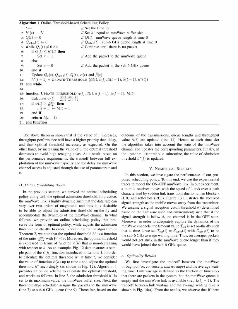
Algorithm 1 Online Threshold-based Scheduling Policy1: t← 1 // Set the time to 12: h∗(t)← K // Set h∗ equal to mmWave buffer size3: Q(t)← 0 // Q(t) : mmWave queue length at time 04: Qsub-6(t)← 0 // Qsub-6(t) : sub-6 GHz queue length at time 05: while Qs(t) 6= 0 do // Continue until there is no packet6: if Q(t) ≤ h∗(t) then7: Set π = 1 // Add the packet to the mmWave queue8: else9: Set π = 0 // Add the packet to the sub-6 GHz queue
10: end if11: Update Qs(t), Qsub-6(t), Q(t), α(t) and β(t)12: h∗(t+ 1) = UPDATE-THRESHOLD
(α(t), β(t), α(t− 1), β(t− 1), h∗(t)
)13: end while14:15: function UPDATE-THRESHOLD(α(t), β(t), α(t− 1), β(t− 1), h(t))16: Calculate ψ(t) = β(t)−β(t−1)
α(t)−α(t−1)
17: if ψ(t) ≥ r+cW+c then
18: h(t+ 1)← h(t)− 119: end if20: return h(t+ 1)21: end function
The above theorem shows that if the value of r increases,throughput performance will have a higher priority than delay,and thus optimal threshold increases, as expected. On theother hand, by increasing the value of c, the optimal thresholddecreases to avoid high reneging costs. As a result, based onthe performance requirements, the tradeoff between full ex-ploitation of the mmWave capacity and the delay for mmWavechannel access is adjusted through the use of parameters r andc.
D. Online Scheduling Policy
In the previous section, we derived the optimal schedulingpolicy along with the optimal admission threshold. In practice,the mmWave link is highly dynamic such that the data rate canvary over two orders of magnitude, and thus it is desirableto be able to adjust the admission threshold on-the-fly andaccommodate the dynamics of the mmWave channel. In whatfollows, we provide an online scheduling policy that pre-serve the form of optimal policy, while adjusts the admissionthreshold on-the-fly. In order to obtain the online algorithm ofTheorem 2, we note that the optimal threshold h∗ is a functionof the ratio r+c
W+c with W ≤ r. Moreover, the optimal thresholdis expressed in terms of function ψ(h) that is non-decreasingwith respect to h. As an example, Fig. 12 demonstrates a sam-ple path of the ψ(h) function introduced in Lemma 1. In orderto calculate the optimal threshold h∗ at time t, we considerthe value of function ψ(h) up to time t and adjust the optimalthreshold h∗ accordingly (as shown in Fig. 12). Algorithm 1provides an online scheme to calculate the optimal threshold,and works as follows. In line 2, the admission threshold h∗ isset to its maximum value, the mmWave buffer size. Next, thethreshold-type scheduler assigns the packets to the mmWave(line 7) or sub-6 GHz queue (line 9). Thereafter, based on the
outcome of the transmissions, queue lengths and throughputvalue α(t) are updated (line 11). Hence, at each time slotthe algorithm takes into account the state of the mmWavechannel and updates the corresponding parameters. Finally, inthe Update-Threshold subroutine, the value of admissionthreshold h∗(t) is updated.
V. NUMERICAL RESULTS
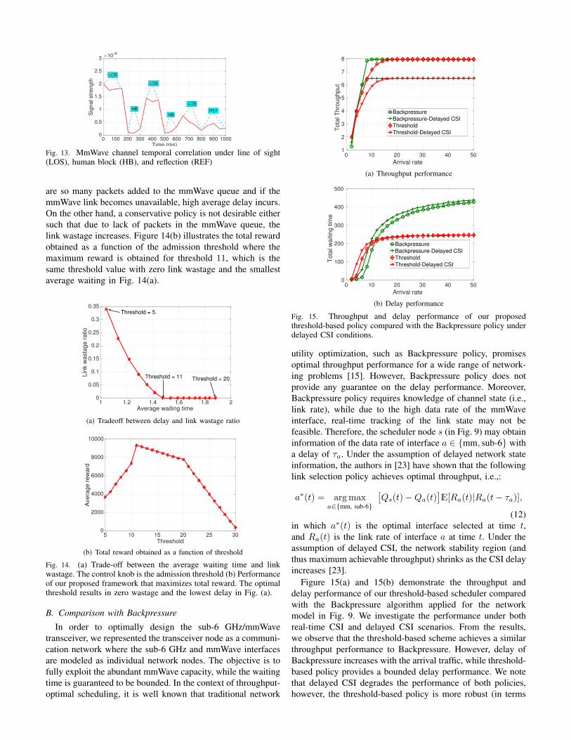
In this section, we investigate the performance of our pro-posed scheduling policy. To this end, we use the experimentaltraces to model the ON-OFF mmWave link. In our experiment,a mobile receiver moves with the speed of 1 m/s over a pathcharacterized by sudden link transitions due to human blockers(HB) and reflectors (REF). Figure 13 illustrates the receivedsignal strength as the mobile moves away from the transmitter.We assume a signal reception cutoff threshold δ (determinedbased on the hardware used and environment) such that if thesignal strength is below δ, the channel is in the OFF state.Moreover, in order to adequately capture the dynamics of themmWave channels, the timeout value Tout is set on-the-fly suchthat at time t, we set Tout(t) = Zsub-6(t) with Zsub-6(t) to bethe sub-6 GHz average waiting time. Thus, on average, packetswould not get stuck in the mmWave queue longer than if theywould have joined the sub-6 GHz queue.
A. Optimality Results
We first investigate the tradeoff between the mmWavethroughput (or, conversely, link wastage) and the average wait-ing time. Link wastage is defined as the fraction of time slotsthat there are packets in the system, but the mmWave queue isempty and the mmWave link is available (i.e., L(t) = 1). Thetradeoff between link wastage and the average waiting time isshown in Fig. 14(a). From the results, we observe that if there
0 100 200 300 400 500 600 700 800 900 1000Time (ms)
0
0.5
1
1.5
2
2.5
3
Sig
nal str
ength
×10-4
LOS
HB
LOS
HB
LOS
REF
Fig. 13. MmWave channel temporal correlation under line of sight(LOS), human block (HB), and reflection (REF)
are so many packets added to the mmWave queue and if themmWave link becomes unavailable, high average delay incurs.On the other hand, a conservative policy is not desirable eithersuch that due to lack of packets in the mmWave queue, thelink wastage increases. Figure 14(b) illustrates the total rewardobtained as a function of the admission threshold where themaximum reward is obtained for threshold 11, which is thesame threshold value with zero link wastage and the smallestaverage waiting in Fig. 14(a).
1 1.2 1.4 1.6 1.8 2Average waiting time
0
0.05
0.1
0.15
0.2
0.25
0.3
0.35
Lin
k w
asta
ge
ra
tio
Threshold = 5
Threshold = 11 Threshold = 20
(a) Tradeoff between delay and link wastage ratio
5 10 15 20 25 30Threshold
0
2000
4000
6000
8000
10000
Avera
ge r
ew
ard
(b) Total reward obtained as a function of threshold
Fig. 14. (a) Trade-off between the average waiting time and linkwastage. The control knob is the admission threshold (b) Performanceof our proposed framework that maximizes total reward. The optimalthreshold results in zero wastage and the lowest delay in Fig. (a).
B. Comparison with Backpressure
In order to optimally design the sub-6 GHz/mmWavetransceiver, we represented the transceiver node as a communi-cation network where the sub-6 GHz and mmWave interfacesare modeled as individual network nodes. The objective is tofully exploit the abundant mmWave capacity, while the waitingtime is guaranteed to be bounded. In the context of throughput-optimal scheduling, it is well known that traditional network
0 10 20 30 40 50
Arrival rate
1
2
3
4
5
6
7
8
Tota
l T
hro
ughput
Backpressure
Backpressure-Delayed CSI
Threshold
Threshold-Delayed CSI
(a) Throughput performance
0 10 20 30 40 50
Arrival rate
0
100
200
300
400
500
Tota
l w
aitin
g tim
e
Backpressure
Backpressure-Delayed CSI
Threshold
Threshold-Delayed CSI
(b) Delay performance
Fig. 15. Throughput and delay performance of our proposedthreshold-based policy compared with the Backpressure policy underdelayed CSI conditions.
utility optimization, such as Backpressure policy, promisesoptimal throughput performance for a wide range of network-ing problems [15]. However, Backpressure policy does notprovide any guarantee on the delay performance. Moreover,Backpressure policy requires knowledge of channel state (i.e.,link rate), while due to the high data rate of the mmWaveinterface, real-time tracking of the link state may not befeasible. Therefore, the scheduler node s (in Fig. 9) may obtaininformation of the data rate of interface a ∈ {mm, sub-6} witha delay of τa. Under the assumption of delayed network stateinformation, the authors in [23] have shown that the followinglink selection policy achieves optimal throughput, i.e.,:
a∗(t) = arg maxa∈{mm, sub-6}
[Qs(t)−Qa(t)
]E[Ra(t)|Ra(t− τa)],
(12)in which a∗(t) is the optimal interface selected at time t,and Ra(t) is the link rate of interface a at time t. Under theassumption of delayed CSI, the network stability region (andthus maximum achievable throughput) shrinks as the CSI delayincreases [23].
Figure 15(a) and 15(b) demonstrate the throughput anddelay performance of our threshold-based scheduler comparedwith the Backpressure algorithm applied for the networkmodel in Fig. 9. We investigate the performance under bothreal-time CSI and delayed CSI scenarios. From the results,we observe that the threshold-based scheme achieves a similarthroughput performance to Backpressure. However, delay ofBackpressure increases with the arrival traffic, while threshold-based policy provides a bounded delay performance. We notethat delayed CSI degrades the performance of both policies,however, the threshold-based policy is more robust (in terms
2 4 6 8 10 12
Arrival rate
1.5
2
2.5
3
3.5
4
4.5
5
Mm
Wave T
hro
ughput
Reneging cost = 1
Reneging cost = 3
Reneging cost = 10
(a) Throughput performance
2 4 6 8 10 12
Arrival rate
0
0.5
1
1.5
2
2.5
3
3.5
Mm
Wave w
aitin
g tim
e
Reneging cost = 1
Reneging cost = 3
Reneging cost = 10
(b) Delay performance
2 4 6 8 10 12
Arrival rate
2
3
4
5
6
Mm
Wave T
hro
ughput
Reward = 2
Reward = 5
Reward = 10
(c) Throughput performance
2 4 6 8 10 12
Arrival rate
0
0.5
1
1.5
2
Mm
Wave w
aitin
g tim
e
Reward = 2
Reward = 5
Reward = 10
(d) Delay performance
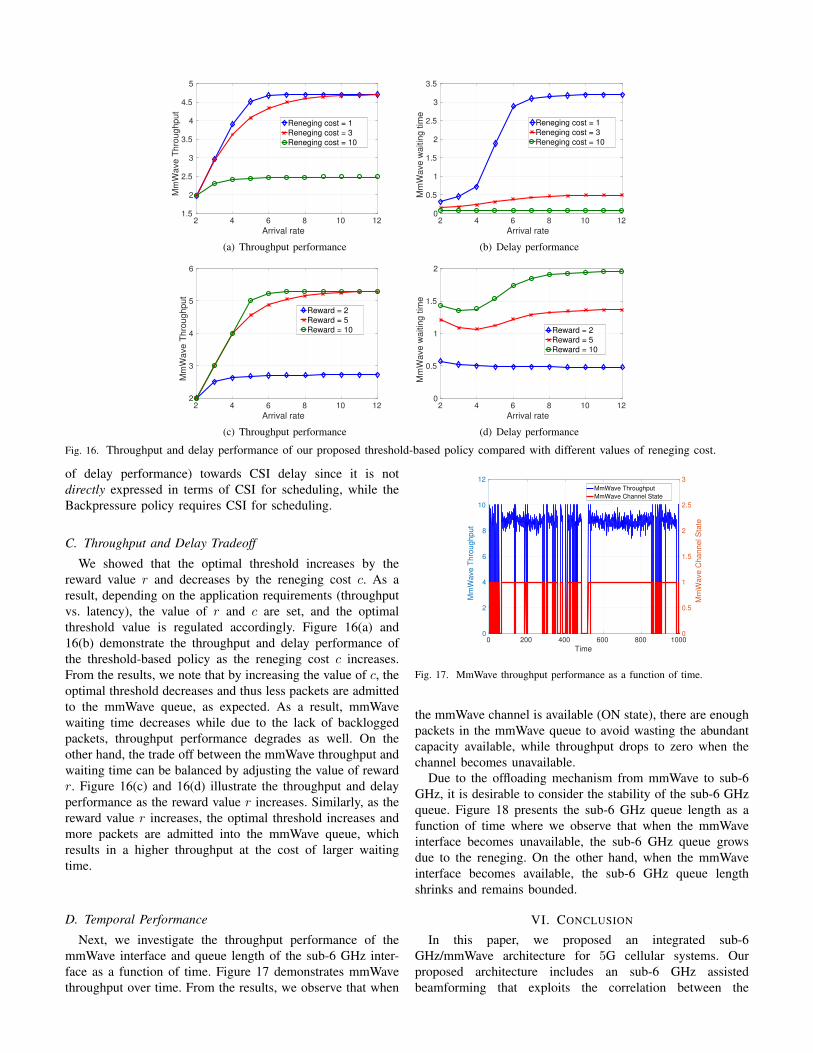
Fig. 16. Throughput and delay performance of our proposed threshold-based policy compared with different values of reneging cost.
of delay performance) towards CSI delay since it is notdirectly expressed in terms of CSI for scheduling, while theBackpressure policy requires CSI for scheduling.
C. Throughput and Delay Tradeoff
We showed that the optimal threshold increases by thereward value r and decreases by the reneging cost c. As aresult, depending on the application requirements (throughputvs. latency), the value of r and c are set, and the optimalthreshold value is regulated accordingly. Figure 16(a) and16(b) demonstrate the throughput and delay performance ofthe threshold-based policy as the reneging cost c increases.From the results, we note that by increasing the value of c, theoptimal threshold decreases and thus less packets are admittedto the mmWave queue, as expected. As a result, mmWavewaiting time decreases while due to the lack of backloggedpackets, throughput performance degrades as well. On theother hand, the trade off between the mmWave throughput andwaiting time can be balanced by adjusting the value of rewardr. Figure 16(c) and 16(d) illustrate the throughput and delayperformance as the reward value r increases. Similarly, as thereward value r increases, the optimal threshold increases andmore packets are admitted into the mmWave queue, whichresults in a higher throughput at the cost of larger waitingtime.
D. Temporal Performance
Next, we investigate the throughput performance of themmWave interface and queue length of the sub-6 GHz inter-face as a function of time. Figure 17 demonstrates mmWavethroughput over time. From the results, we observe that when
0 200 400 600 800 1000
Time
0
2
4
6
8
10
12
Mm
Wa
ve
Th
rou
gh
pu
t
0
0.5
1
1.5
2
2.5
3
Mm
Wa
ve
Ch
an
ne
l S
tate
MmWave Throughput
MmWave Channel State
Fig. 17. MmWave throughput performance as a function of time.
the mmWave channel is available (ON state), there are enoughpackets in the mmWave queue to avoid wasting the abundantcapacity available, while throughput drops to zero when thechannel becomes unavailable.
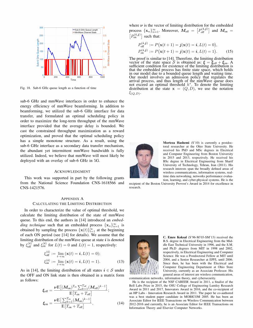
Due to the offloading mechanism from mmWave to sub-6GHz, it is desirable to consider the stability of the sub-6 GHzqueue. Figure 18 presents the sub-6 GHz queue length as afunction of time where we observe that when the mmWaveinterface becomes unavailable, the sub-6 GHz queue growsdue to the reneging. On the other hand, when the mmWaveinterface becomes available, the sub-6 GHz queue lengthshrinks and remains bounded.
VI. CONCLUSION
In this paper, we proposed an integrated sub-6GHz/mmWave architecture for 5G cellular systems. Ourproposed architecture includes an sub-6 GHz assistedbeamforming that exploits the correlation between the
0 200 400 600 800 1000
Time
0
50
100
150
200
250
300
Su
b-6
GH
z Q
ue
ue
Le
ng
th
0
0.5
1
1.5
2
2.5
3
Mm
Wa
ve
Ch
an
ne
l S
tate
Sub-6 GHz Queue Length
MmWave Channel State
Fig. 18. Sub-6 GHz queue length as a function of time
sub-6 GHz and mmWave interfaces in order to enhance theenergy efficiency of mmWave beamforming. In addition tobeamforming, we utilized the sub-6 GHz interface for datatransfer, and formulated an optimal scheduling policy inorder to maximize the long-term throughput of the mmWaveinterface provided that the average delay is bounded. Wecast the constrained throughput maximization as a rewardoptimization, and proved that the optimal scheduling policyhas a simple monotone structure. As a result, using thesub-6 GHz interface as a secondary data transfer mechanism,the abundant yet intermittent mmWave bandwidth is fullyutilized. Indeed, we believe that mmWave will most likely bedeployed with an overlay of sub-6 GHz in 5G.
ACKNOWLEDGMENT
This work was supported in part by the following grantsfrom the National Science Foundation CNS-1618566 andCNS-1421576.
APPENDIX ACALCULATING THE LIMITING DISTRIBUTION
In order to characterize the value of optimal threshold, wecalculate the limiting distribution of the state of mmWavequeue. To this end, the authors in [14] introduced an embed-ding technique such that an embedded process {xn}∞n=1 isobtained by sampling the process {x(t)}∞t=1 at the beginningof each ON period (see [14] for details). We assume that thelimiting distribution of the mmWave queue at state i is denotedby ξ(i)
off and ξ(i)on for L(t) = 0 and L(t) = 1, respectively:
ξ(i)off := lim
t→∞(x(t) = i, L(t) = 0);
ξ(i)on := lim
t→∞(x(t) = i, L(t) = 1). (13)
As in [14], the limiting distribution of all states i ∈ S underthe OFF and ON link state is then obtained in a matrix formas follows:
ξoff =νE[(Mon)Ton
∑Toffk=1(Moff)
k−1]
E[Ton + Toff
] ;
ξon =νE[∑Ton
k=1(Mon)k−1]
E[Ton + Toff
] , (14)
where ν is the vector of limiting distribution for the embeddedprocess {xn}∞n=1. Moreover, Moff =
[P
(i,j)off
]and Mon =[
P(i,j)on
]such that:
P(i,j)off := P
(x(t+ 1) = j|x(t) = i, L(t) = 0
),
P (i,j)on := P
(x(t+ 1) = j|x(t) = i, L(t) = 1
). (15)
The proof is similar to [14]. Therefore, the limiting distributionvector of the state space S is obtained as: ξ = ξoff + ξon. Asufficient condition for existence of the limiting distribution isthat the embedded process has finite state space, which holdsin our model due to a bounded queue length and waiting time.Our model involves an admission policy that regulates thearrival process, and thus length of the mmWave queue doesnot exceed an optimal threshold h∗. To denote the limitingdistribution at the state x = (Q,D), we use the notationξ(Q,D).
Morteza Hashemi (S’10) is currently a postdoc-toral researcher at the Ohio State University. Hereceived his PhD and MSc degrees in Electricaland Computer Engineering from Boston Universityin 2015 and 2013, respectively. He received hisBSc degree in Electrical Engineering from SharifUniversity of Technology, Tehran, Iran (2011). Hisresearch interests span the broadly defined areas ofwireless communications, information systems, real-time data networking, networks performance evalua-tion, learning, and cyber-physical systems. He is the
recipient of the Boston University Provost’s Award in 2014 for excellence inresearch.
C. Emre Koksal (S’96-M’03-SM’13) received theB.S. degree in Electrical Engineering from the Mid-dle East Technical University in 1996, and the S.M.and Ph.D .degrees from MIT in 1998 and 2002,respectively, in Electrical Engineering and ComputerScience. He was a Postdoctoral Fellow at MIT until2004, and a Senior Researcher at EPFL until 2006.Since then, he has been with the Electrical andComputer Engineering Department at Ohio StateUniversity, currently as an Associate Professor. Hisgeneral areas of interest are wireless communication,
communication networks, information theory, and cybersecurity.He is the recipient of the NSF CAREER Award in 2011, a finalist of the
Bell Labs Prize in 2015, the OSU College of Engineering Lumley ResearchAward in 2011 and 2017, Innovators Award in 2016, and the co-recipient ofan HP Labs - Innovation Research Award in 2011. The paper he co-authoredwas a best student paper candidate in MOBICOM 2005. He has been anAssociate Editor for IEEE Transactions on Wireless Communication between2012-2016 and currently, he is an Associate Editor for IEEE Transactions onInformation Theory and Elsevier Computer Networks.
Ness B. Shroff (S’91-M’93-SM’01-F’07) receivedhis Ph.D. degree in Electrical Engineering fromColumbia University in 1994. He joined Purdueuniversity immediately thereafter as an AssistantProfessor in the school of ECE. At Purdue, hebecame Full Professor of ECE in 2003 and directorof CWSA in 2004, a university-wide center onwireless systems and applications. In July 2007, hejoined The Ohio State University, where he holds theOhio Eminent Scholar endowed chair in Networkingand Communications, in the departments of ECE and
CSE. He holds or has held visiting (chaired) professor positions at TsinghuaUniversity, Beijing, China, Shanghai Jiaotong University, Shanghai, China,and the Indian Institute of Technology, Bombay, India. Dr. Shroff is currentlyan editor at large of IEEE/ACM Trans. on Networking, senior editor of IEEETransactions on Control of Networked Systems, and technical editor for theIEEE Network Magazine. He has received numerous best paper awards for hisresearch and listed Thomson Reuters Book on The World’s Most InfluentialScientific Minds as well as noted as a highly cited researcher by ThomsonReuters. He also received the IEEE INFOCOM achievement award for seminalcontributions to scheduling and resource allocation in wireless networks.
REFERENCES
[1] F. Khan and Z. Pi, “mmWave mobile broadband (MMB): Unleashingthe 3–300GHz spectrum,” in 34th IEEE Sarnoff Symposium, 2011.
[2] T. S. Rappaport, S. Sun, R. Mayzus, H. Zhao, Y. Azar, K. Wang, G. N.Wong, J. K. Schulz, M. Samimi, and F. Gutierrez, “Millimeter wavemobile communications for 5G cellular: It will work!” Access, IEEE,vol. 1, pp. 335–349, 2013.
[3] W. Roh, J.-Y. Seol, J. Park, B. Lee, J. Lee, Y. Kim, J. Cho, K. Cheun, andF. Aryanfar, “Millimeter-wave beamforming as an enabling technologyfor 5G cellular communications: theoretical feasibility and prototyperesults,” IEEE Communications Magazine, vol. 52, no. 2, 2014.
[4] J. Mo, A. Alkhateeb, S. Abu-Surra, and R. W. Heath Jr, “Hybridarchitectures with few-bit ADC receivers: Achievable rates and energy-rate tradeoffs,” arXiv preprint arXiv:1605.00668, 2016.
[5] T. Nitsche, A. B. Flores, E. W. Knightly, and J. Widmer, “Steering witheyes closed: mm-wave beam steering without in-band measurement,” inComputer Communications (INFOCOM), IEEE Conference on. IEEE,2015, pp. 2416–2424.
[6] A. Ali, N. Prelcic, and R. Heath, “Estimating millimeter wave channelsusing out-of-band measurements,” Information Theory and ApplicationsWorkshop (ITA), 2016.
[7] M. Hashemi, C. E. Koksal, and N. B. Shroff, “Hybrid RF-mmWavecommunications to achieve low latency and high energy efficiency in 5Gcellular systems,” in Modeling and Optimization in Mobile, Ad Hoc, andWireless Networks (WiOpt), 15th International Symposium on. IEEE,2017.
[8] S. Collonge, G. Zaharia, and G. E. Zein, “Influence of the human activityon wide-band characteristics of the 60 GHz indoor radio channel,”Wireless Communications, IEEE Transactions on, vol. 3, no. 6, pp.2396–2406, 2004.
[9] S. Rangan, T. S. Rappaport, and E. Erkip, “Millimeter-wave cellularwireless networks: Potentials and challenges,” Proceedings of the IEEE,vol. 102, no. 3, pp. 366–385, 2014.
[10] T. S. Rappaport, R. W. Heath Jr, R. C. Daniels, and J. N. Murdock,Millimeter wave wireless communications. Pearson Education, 2014.
[11] V. Nurmela, A. Karttunen, A. Roivainen, L. Raschkowski, T. Imai,J. Jarvelainen, J. Medbo, J. Vihriala, J. Meinila, K. Haneda et al.,“METIS channel models,” Seventh FrameworN Programme ICT-317669,2015.
[12] A. Adhikary, E. Al Safadi, M. K. Samimi, R. Wang, G. Caire, T. S.Rappaport, and A. F. Molisch, “Joint spatial division and multiplexingfor mm-wave channels,” IEEE Journal on Selected Areas in Communi-cations, vol. 32, no. 6, pp. 1239–1255, 2014.
[13] A. Ali, N. Gonzalez-Prelcic, and R. W. Heath Jr, “Millimeter wavebeam-selection using out-of-band spatial information,” arXiv preprintarXiv:1702.08574, 2017.
[14] Y. Kim, K. Lee, and N. B. Shroff, “An analytical framework tocharacterize the efficiency and delay in a mobile data offloading system,”in Proceedings of the 15th ACM international symposium on Mobile adhoc networking and computing. ACM, 2014, pp. 267–276.
[15] L. Georgiadis, M. J. Neely, and L. Tassiulas, Resource allocation andcross-layer control in wireless networks. Now Publishers Inc, 2006.
[16] M. Alresaini, M. Sathiamoorthy, B. Krishnamachari, and M. J. Neely,“Backpressure with adaptive redundancy (BWAR),” in INFOCOM, 2012Proceedings IEEE. IEEE, 2012, pp. 2300–2308.
[17] X. L. Bui, E. Athanasopoulou, T. Ji, R. Srikant, and A. Stolyar,“Backpressure-based packet-by-packet adaptive routing in communica-tion networks,” 2012.
[18] B. Ji, C. Joo, and N. B. Shroff, “Delay-based back-pressure schedulingin multihop wireless networks,” IEEE/ACM Transactions on Networking(TON), vol. 21, no. 5, pp. 1539–1552, 2013.
[19] J. G. Andrews, T. Bai, M. Kulkarni, A. Alkhateeb, A. Gupta, and R. W.Heath Jr, “Modeling and analyzing millimeter wave cellular systems,”arXiv preprint arXiv:1605.04283, 2016.
[20] R. Schmidt, “Multiple emitter location and signal parameter estimation,”IEEE transactions on antennas and propagation, vol. 34, no. 3, pp. 276–280, 1986.
[21] M. L. Puterman, Markov decision processes: discrete stochastic dynamicprogramming. John Wiley & Sons, 2014.
[22] M. Larranaga, O. J. Boxma, R. Nunez-Queija, and M. S. Squillante, “Ef-ficient content delivery in the presence of impatient jobs,” in TeletrafficCongress (ITC 27), 27th International. IEEE, 2015, pp. 73–81.
[23] L. Ying and S. Shakkottai, “On throughput optimality with delayednetwork-state information,” IEEE Transactions on Information Theory,vol. 57, no. 8, pp. 5116–5132, 2011.