ABCDEFG

UNIVERSITY OF OULU P .O. B 00 F I -90014 UNIVERSITY OF OULU FINLAND

A C T A U N I V E R S I T A T I S O U L U E N S I S

S E R I E S E D I T O R S

SCIENTIAE RERUM NATURALIUM

HUMANIORA

TECHNICA

MEDICA

SCIENTIAE RERUM SOCIALIUM

SCRIPTA ACADEMICA

OECONOMICA

EDITOR IN CHIEF

PUBLICATIONS EDITOR

Professor Esa Hohtola

University Lecturer Santeri Palviainen

Postdoctoral research fellow Sanna Taskila

Professor Olli Vuolteenaho

University Lecturer Veli-Matti Ulvinen

Director Sinikka Eskelinen

Professor Jari Juga

Professor Olli Vuolteenaho

Publications Editor Kirsti Nurkkala

ISBN 978-952-62-0657-8 (Paperback)ISBN 978-952-62-0658-5 (PDF)ISSN 0355-3213 (Print)ISSN 1796-2226 (Online)

U N I V E R S I TAT I S O U L U E N S I SACTAC

TECHNICA

U N I V E R S I TAT I S O U L U E N S I SACTAC

TECHNICA

OULU 2014

C 510

Pertti Ala-aho

GROUNDWATER-SURFACE WATER INTERACTIONS IN ESKER AQUIFERSFROM FIELD MEASUREMENTS TO FULLY INTEGRATED NUMERICAL MODELLING

UNIVERSITY OF OULU GRADUATE SCHOOL;UNIVERSITY OF OULU,FACULTY OF TECHNOLOGY

C 510

ACTA

Pertti Ala-aho

C510etukansi.kesken.fm Page 1 Thursday, October 30, 2014 3:11 PM

A C T A U N I V E R S I T A T I S O U L U E N S I SC Te c h n i c a 5 1 0

PERTTI ALA-AHO

GROUNDWATER-SURFACE WATER INTERACTIONS IN ESKER AQUIFERSFrom field measurements to fully integrated numerical modelling

Academic dissertation to be presented with the assent ofthe Doctoral Training Committee of Technology andNatural Sciences of the University of Oulu for publicdefence in Auditorium GO101, Linnanmaa, on 9December 2014, at 12 noon

UNIVERSITY OF OULU, OULU 2014

Copyright © 2014Acta Univ. Oul. C 510, 2014

Supervised byProfessor Bjørn Kløve

Reviewed byProfessor Peter EngesgaardDoctor Jon Paul Jones

ISBN 978-952-62-0657-8 (Paperback)ISBN 978-952-62-0658-5 (PDF)

ISSN 0355-3213 (Printed)ISSN 1796-2226 (Online)

Cover DesignRaimo Ahonen

JUVENES PRINTTAMPERE 2014

OpponentProfessor Philip Brunner

Ala-aho, Pertti, Groundwater-surface water interactions in esker aquifers. Fromfield measurements to fully integrated numerical modellingUniversity of Oulu Graduate School; University of Oulu, Faculty of TechnologyActa Univ. Oul. C 510, 2014University of Oulu, P.O. Box 8000, FI-90014 University of Oulu, Finland

Abstract

Water resources management calls for methods to simultaneously manage groundwater (GW) andsurface water (SW) systems. These have traditionally been considered separate units of thehydrological cycle, which has led to oversimplification of exchange processes at the GW-SWinterface. This thesis studied GW hydrology and the previously unrecognised connection of theRokua esker aquifer with lakes and streams in the area, with the aim of identifying reasons for lakewater level variability and eutrophication in the Rokua esker.

GW-SW interactions in the aquifer were first studied with field methods. Seepage metermeasurements showed substantial spatial variability in GW-lake interaction, whereas transientvariability was more modest, although present and related to the surrounding aquifer.Environmental tracers suggested that water exchange occurs in all lakes in the area, but is ofvarying magnitude in different lakes. Finally, GW-SW interaction was studied in peatlandcatchments, where drainage channels in the peat soil presumably increased groundwater outflowfrom the aquifer.

Amount and rate of GW recharge were then estimated with a simulation approach developedexplicitly to account for the physical characteristics of the Rokua esker aquifer. This produced aspatially and temporally distributed recharge estimate, which was validated by independent fieldtechniques. The results highlighted the impact of canopy characteristics, and thereby forestrymanagement, on GW recharge.

The data collected and the new understanding of site hydrology obtained were refined into afully integrated surface-subsurface flow model of the Rokua aquifer. Simulation results comparedfavourably to field observations of GW, lake levels and stream discharge. A major finding was ofgood agreement between simulated and observed GW inflow to lakes in terms of dischargelocations and total influx.

This thesis demonstrates the importance of using multiple methods to gain a comprehensiveunderstanding of esker aquifer hydrology with interconnected lakes and streams. Importantly, site-specific information on the reasons for water table variability and the trophic status of Rokualakes, which is causing local concern, is provided. As the main outcome, various field andmodelling methods were tested, refined and shown to be suitable for integrated GW and SWresource management in esker aquifers.

Keywords: environmental tracers, esker aquifers, groundwater, groundwater-surfacewater interaction, hydrological modelling

Ala-aho, Pertti, Pinta- ja pohjaveden vuorovaikutus harjuakvifereissa. Kenttämit-tauksista integroituun numeeriseen mallinnukseenOulun yliopiston tutkijakoulu; Oulun yliopisto, Teknillinen tiedekuntaActa Univ. Oul. C 510, 2014Oulun yliopisto, PL 8000, 90014 Oulun yliopisto

Tiivistelmä

Vesivarojen hallinnassa tarvitaan menetelmiä pohja- ja pintaveden kokonaisvaltaiseen huomioi-miseen. Pohja- ja pintavesiä tarkastellaan usein erillisinä osina hydrologista kiertoa, mikä onjohtanut niiden välisten virtausprosessien yksinkertaistamiseen. Tässä työssä selvitettiin Rokuanpohjavesiesiintymän hydrologiaa ja hydraulista yhteyttä alueella oleviin järviin ja puroihin. Tut-kimuksessa pyrittiin osaltaan selvittämään syitä harjualueen järvien pinnanvaihteluun ja vedenlaatuongelmiin.

Kenttätutkimuksissa todettiin voimakasta alueellista vaihtelua järven ja pohjaveden vuoro-vaikutuksessa. Pohjaveden suotautumisen ajallinen vaihtelu puolestaan oli vähäisempää, muttahavaittavissa, ja kytköksissä järveä ympäröivän pohjavesipinnan vaihteluihin. Merkkiaineetvesinäytteistä viittasivat vastaavan vuorovaikutuksen olevan läsnä myös muissa alueen järvissä,mutta suotautuvan pohjaveden määrän vaihtelevan järvittäin. Turvemailla tehdyt mittauksetosoittivat pohjaveden purkautuvan ojaverkostoon ja ojituksen mahdollisesti lisäävän ulosvirtaa-maa pohjavesiesiintymästä.

Pohjaveden muodostumismäärää ja -nopeutta tutkittiin numeerisella mallinnuksella, jokakehitettiin huomioimaan harjualueelle ominaiset fysikaaliset tekijät. Mallinnus tuotti arvion ajal-lisesti ja alueellisesti vaihtelevasta pohjaveden muodostumisesta, joka varmennettiin kenttämit-tauksilla. Tuloksissa korostui kasvillisuuden, ja sitä kautta metsähakkuiden, vaikutus pohjave-den muodostumismääriin.

Hydrologiasta kerätyn aineiston ja kehittyneen prosessiymmärryksen avulla Rokuan harju-alueesta muodostettiin täysin integroitu numeerinen pohjavesi-pintavesi virtausmalli. Mallinnus-tulokset vastasivat mittauksia pohjaveden ja järvien pinnantasoista sekä purovirtaamista. Työnmerkittävin tulos oli, että mallinnetut pohjaveden purkautumiskohdat ja purkautumismäärät alu-een järviin vastasivat kenttähavaintoja.

Tämä työ havainnollisti, että ymmärtääkseen pohjaveden ja siitä riippuvaisten järvien japurojen vuorovaikutusta harjualueella on käytettävä monipuolisia tutkimusmenetelmiä. Työ toilisätietoa Rokuan harjualueen vesiongelmien syihin selittäen järvien vedenpinnan vaihtelua javedenlaatua pohjavesihydrologialla. Väitöstyön tärkein anti oli erilaisten kenttä- ja mallinnus-menetelmien soveltaminen, kehittäminen ja hyödylliseksi havaitseminen harjualueiden koko-naisvaltaisessa pinta- ja pohjavesien hallinnassa.

Asiasanat: harjut, hydrologinen mallinnus, pinta- ja pohjaveden vuorovaikutus,pohjavesi, ympäristömerkkiaineet

To my Mother

8

9

Acknowledgements

This thesis was made possible by funding from the EU Seventh Framework

Programme GENESIS (no. 226536) and the Academy of Finland project AQVI (no.

128377). In addition, VALUE doctoral programme, Thule doctoral programme and

University of Oulu Graduate School offered high level education, scientific

workshops and travel grants, which gave me the knowhow required for the thesis. In

addition, travel and personal grants from Maa- ja Vesitekniikan Tuki r.y., Renlund

Foundation, Tauno Tönning Foundation and Sven Hallin Foundation were vital in

completing the thesis and giving me the opportunity to attend several international

scientific courses, conferences and an exchange visit.

My supervisor, Prof. Bjørn Kløve, gets my sincerest gratitude for guiding me

through the PhD process and creating unique opportunities during that time. I

especially appreciate the open-mindedness and encouraging attitude of Prof. Kløve,

which gave me great support in becoming a scientist. Another person who single-

handedly made a tremendous contribution to this thesis was my dear friend and

colleague Pekka Rossi. Innumerable shared moments and experiences made these

years what they were, cheers mate! I thank pre-examiners Dr. John Paul Jones and

Prof. Peter Engesgaard for their valuable contribution in completing the thesis and Dr.

Mary McAfee for her expertise and helpfulness in language revision of all the

manuscripts.

My day-to-day work at the university was always coloured by the Water

Resources and Environmental Engineering Research Group - thank you all for the

shared laughs and help I could always rely on. I want to thank Anna-Kaisa, Elina,

Hannu, Riku, Virve K., Tuomo R., and Tuomo P. for their important contributions to

the thesis, and (going from south to north along our corridor) Virve M, Ali, Pirkko,

Katharina, Jarmo, Anne, Kauko, Simo, Paavo, Shähram, Tuomas, Masoud, Tapio,

Ehsan, Meseret, Justice, Elisangela, Heini, and all the trainees and students over the

years for their smiles and kind words.

I had the privilege to spend fall semester 2012 at the University of Waterloo,

Canada, which was crucial for the final outcome of this thesis. I sincerely thank all the

inspiring professors, students and people at UW and Aquanty Inc. Special thanks to

Prof. Ed Sudicky and his team at the time, Rob, Young-Jin, Hyuon-Tae and Jason, for

their help with the HGS and hospitality in general. Several other institutions and

collaborators have provided irreplaceable input to this thesis and sincere thanks go to

all those individuals and institutions who took part in investigations at the Rokua site.

In particular would like to thank Jarkko Okkonen for his advice and discussions along

10

the way, which gave me lots of perspective and new ideas. I want to acknowledge all

the people in the GENESIS project for their great scientific advice and fun company

in the memorable meetings around Europe. You are too many to list, sorry! As seen

from the above, this four-year period acquainted me with numerous people around the

world, for which I’m extremely grateful. Special thanks to Dmytro, Marc-André and

Peter, my international friends, it has been a pleasure getting to know you guys.

An unconditional thank you goes to my family Tuija, Olavi, Irma, Laura, Saara,

Vilma and extended family and friends, who have been my bedrock throughout my

studies. Dear sisters, read the next hundred or so pages and you might finally figure

out what it is I do at the University. Sweet thank you Essi-Maaria for your loving

encouragement and support.

Even though my name appears on the book cover, it is just as much authored by

all the people acknowledged above and the science preceding my studies. You gave

small ideas like springs, which eventually combined into the stream flowing in the

text. My humble thanks to you all.

Oulu, October 2014 Pertti Ala-aho

11

List of symbols and abbreviations

GW-SW Groundwater – surface water

SWE Snow water equivalent

asl Above sea level

K Hydraulic conductivity of porous medium

MH Finnish Forest Administration (Metsähallitus)

MK Finnish Forest Centre (Metsäkeskus)

EC Electrical conductivity, a water quality parameter

LAI Leaf area index

UZD Unsaturated zone depth

1-D One-dimensional

DEM Digital elevation model

TIR Thermal infrared imaging

B&C Brooks and Corey water retention function

WTF Water table fluctuation method to estimate groundwater recharge

ELY Centre Centre for Economic Development, Transport and the Environment

FMI Finnish Meteorological Institute

12

13

List of original publications

This thesis is based on the following publications, which are referred to throughout

the text by their Roman numerals:

I Ala-aho P, Rossi, PM & Kløve, B (2013) Interaction of esker groundwater with headwater lakes and streams. Journal of Hydrology 500(2013): 144-156.

II Rossi PM, Ala-aho P, Ronkanen A-K & Kløve B (2012) Groundwater-surface water interaction between an esker aquifer and a drained fen. Journal of Hydrology 432-433 (2012): 52-60.

III Ala-aho P, Rossi, PM & Kløve, B (2014) Estimation of temporal and spatial variations in groundwater recharge in unconfined sand aquifers using Scots pine inventories. Hydrology and Earth System Sciences Discussions 11: 7773-7826. (Manuscript)

IV Ala-aho P, Rossi, PM, Isokangas E & Kløve, B (2014) Fully integrated surface-subsurface flow modelling of groundwater-lake interaction in an esker aquifer: Model verification with stable isotopes and airborne thermal imaging. (Manuscript)

The author’s contribution to publications I-IV:

I Designed the study with co-authors. Performed the field work and analysed the results with Pekka Rossi. Wrote the paper with the co-authors.

II Designed the study with Pekka Rossi and Bjørn Kløve, conducted the field work with Pekka Rossi. Analysed the results and wrote the paper with the co-authors.

III Designed the study with the co-authors. Conducted the field work with Pekka Rossi. Was responsible for the modelling work, data analysis and writing the paper. Received critical comments on model analysis and on the manuscript from the co-authors.

IV Designed the study with Pekka Rossi and Bjørn Kløve. Conducted the field work with Pekka Rossi and Elina Isokangas. Took responsibility for the modelling work. Received critical comments on model analysis and wrote the manuscript with the co-authors.

14

15

Contents

Abstract

Tiivistelmä

Acknowledgements 9 

List of symbols and abbreviations 11 

List of original publications 13 

Contents 15 

1  Introduction 17 

1.1  Future trends in Finnish groundwater management ................................ 17 

1.2  Towards integrated management of GW and SW ................................... 18 

1.3  Research questions and objectives .......................................................... 20 

2  Interactions between groundwater and surface water 23 

3  Study site: Rokua esker aquifer 29 

3.1  Hydrogeological characteristics .............................................................. 29 

3.2  Data collection network .......................................................................... 32 

4  Materials and methods 41 

4.1  Field methods to study GW-SW interactions .......................................... 41 

4.1.1  Seepage meter measurements (I) .................................................. 41 

4.1.2  Hydraulic measurements in the peatland drainage network (II) ... 44 

4.1.3  Environmental tracers (I & II) ...................................................... 47 

4.1.4  Airborne thermal infrared imaging (IV) ....................................... 48 

4.2  Simulations for spatially and temporally distributed recharge (III) ........ 50 

4.2.1  Vegetation and unsaturated zone parameterisation ....................... 50 

4.2.2  Simulation framework .................................................................. 52 

4.3  Fully integrated surface-subsurface flow modelling (IV) ....................... 57 

4.3.1  Model application to Rokua esker aquifer .................................... 57 

4.3.2  Model calibration and validation .................................................. 61 

5  Results and discussion 63 

5.1  Field measurements to verify GW-SW interactions ................................ 63 

5.1.1  Interaction based on flux and hydraulic gradient (I & II) ............. 63 

5.1.2  Environmental tracers at aquifer and water body scale (I & II) ... 69 

5.1.3  Airborne thermal infrared imaging (IV) ....................................... 75 

5.1.4  Conceptual model for GW-SW interactions ................................. 76 

5.2  Spatially and temporally distributed groundwater recharge (III) ............ 78 

5.2.1  Model validation ........................................................................... 79 

5.2.2  Spatially and temporally distributed recharge time series ............ 80 

16

5.2.3  Impact of LAI on groundwater recharge ...................................... 83 

5.3  Surface-subsurface flow modelling of GW-lake interactions (IV) ......... 85 

5.3.1  GW-lake interaction: discharge locations and fluxes ................... 86 

5.3.2  Simulated transient variability in the GW-lake interaction .......... 90 

6  Conclusions and future recommendations 95 

References 99 

Appendices 111 

Original publications 113 

17

1 Introduction

1.1 Future trends in Finnish groundwater management

Groundwater resources are vital for the well-being of society by providing a clean and

reliable freshwater source for human consumption and agriculture, while supporting

ecosystem services. However, these resources are facing multiple stresses at present,

which are likely to increase in the future. The main threats come from over-

abstraction (Konikow & Kendy 2005, Wada et al. 2010), pollution (Gleick 1993,

Spalding & Exner 1993) and climate change (Green et al. 2011, Holman 2006,

Treidel et al. 2011), all acting together to make the use of global groundwater

resources less reliable in a world with a growing population and increasing need for

water. As a consequence, groundwater management agencies and legislation have to

respond to these challenges worldwide. Even though global trends in stressors are

evident, local water resource management has to address aquifer-specific problems. In

Finland, water resources management is guided by the National Water Act (Ministry

of the Environment 2004) and European Union Groundwater Directive (EC 2006),

both aiming to ensure the qualitative and quantitative integrity of groundwater bodies

and related ecosystems.

To date, the Finnish policy for providing water supply has preferred the use of

groundwater over surface water as a more clean and reliable water source (Katko et al. 2006). Unconfined esker aquifers make up the majority of exploitable groundwater

resources for large-scale water supply in Finland (Britschgi et al. 2009). The total

volume of renewable groundwater in esker aquifers greatly exceeds Finnish

requirements, but the resources are small in size and unevenly distributed (Isomäki et al. 2007). The small and unconfined aquifers are susceptible to contamination, and the

number of aquifers at risk of contamination has markedly increased within recent

years (Ministry of the Environment 2013). Eskers are commonly covered by

peatlands in their groundwater discharge area. These peatlands are often drained for

forestry, but groundwater exfiltration to peatlands is not well understood (Langhoff et al. 2006, Lowry et al. 2009), which brings about uncertainty in land use management

around esker aquifers.

Management of conflicting interests around these complex aquifers has gained

recent research attention (Bolduc et al. 2005, Karjalainen et al. 2013, Koundouri et al. 2012, Kurki et al. 2013). As growing communities in Finland demand more potable

groundwater, increasing abstraction pressures along with threats from contamination

18

have generated plans to exploit aquifers in Natura 2000 natural conservation areas

(Isomäki et al. 2007). In addition to water supply, esker aquifers support

groundwater-dependent ecosystems and provide recreational services for local

inhabitants (Kløve et al. 2011). Finnish water abstraction plans have brought about

vibrant discussion and, in some cases, strong local opposition to abstraction that

might endanger protected natural habitats dependent on groundwater. A major reason

igniting the conflicts has been uncertainty about the impacts of water abstraction on

surface water bodies and on ecological systems dependent on the groundwater

outflow.

At the same time, there has been a clear shift in management focus: well-being of

aquatic ecosystems is now at the centre of European Union (EU) water management

(EC 2000). One particularly important and endangered ecosystem type is

groundwater-dependent ecosystems (GDEs), and the EU Groundwater Directive

requires such systems to be characterised in order to determine their quality status

(EC 2006). GDEs can be found in water bodies such as springs, wetlands, rivers and

lakes, where groundwater directly or indirectly sustains ecosystems by providing

them with a favourable water flow, temperature or chemical environment (Kløve et al. 2011). However, in most cases there is very little information on the status or even

existence of GDEs or the environmental conditions they require (Brown et al. 2010,

Hinsby et al. 2008).

Knowledge about GDEs is particularly important in Finland due to plans to

include GDEs as a part of the national classification of exploitable aquifers

(Government of Finland 2014). This would mean that the protected status of aquifers

would partly depend on the ecosystems they support, and thereby influence land use

planning and abstraction regulation. Such proposed legislation generates an urgent

need to develop new tools and to raise awareness about existing practical methods for

distinguishing, monitoring and protecting GDEs (Bertrand et al. 2013, Kløve et al. 2011). A key factor here is groundwater input to surface water bodies, which needs to

be better understood and quantified. Groundwater and surface water should be

considered as one management unit, because they are both highly relevant and

interlinked in creating environmental conditions for biological communities (Hayashi

& Rosenberry 2002, Katko et al. 2006, Sophocleous 2002, Winter et al. 1998).

1.2 Towards integrated management of GW and SW

Groundwater (GW) and surface water (SW) are interlinked parts of the hydrological

cycle, but are often erroneously treated as individual components. In reality, they

19

interact in most landscapes and climates. The main reason for ignoring the interaction

between these to date has been lack of a conceptual process understanding and

technical shortcomings. As Winter et al. (1998) put it: “Surface water is commonly hydraulically connected to groundwater, but the interactions are difficult to observe and measure”.

Winter (1995) summarises GW-SW interaction studies over their 100-year

history, from aquifer contribution to streamflow in early studies, moving in the 1960s

to groundwater and lake environments due to acid rain and eutrophication, and

expanding to wetlands and estuaries because of loss of ecosystems in the 1980s. A

final spurt in the number of GW-SW studies appeared in the 1990s, when the work

focused on physical and biochemical process understanding (Sophocleous 2002).

Increased process understanding and technological advances during recent

decades have generated numerous GW-SW interaction measurement techniques

covering a wide array of temporal and spatial scales (Kalbus et al. 2006, Rosenberry

& LaBaugh 2008). The underlying message from these studies is that water exchange

between groundwater and surface water is highly transient in time and variable in

space and is controlled by numerous interconnected features and processes, such as

subsurface heterogeneities, groundwater flow systems, microtopography of the

surface water bed, climate conditions and near-shore vegetation. In this regard, even

though process understanding has markedly increased and novel technologies have

offered a variety of tools to measure the interaction, the message in Winter et al. (1998) still holds; because of process complexity, measuring GW-SW interactions is

difficult.

The research question as regards GW-SW interactions is moving from how to measure towards how to manage. Water resources management commonly operates

on large (watershed or aquifer) scale, but processes at the GW-SW interface can be

found on metre scale and revealed only with laborious measurements. In addition,

several techniques are commonly needed to obtain an adequate process understanding

of GW-SW interactions at a given study site (Bertrand et al. 2013). Even with various

methods, it can be difficult to transform and extrapolate information across scales

(Krause et al. 2014, Smith et al. 2008, Sophocleous 2002). A major research question

is thus how to produce information of relevant spatial and temporal resolution in order

to facilitate integrated management of water resources and ecosystems.

20

1.3 Research questions and objectives

The work presented in this thesis was conducted to gain a comprehensive

understanding of hydrological processes in the Rokua esker aquifer in Finland and to

provide tools for integrated water resources management for Rokua and esker aquifers

in general. The primary focus was to reveal the anticipated, but yet unknown,

connections between groundwater and surface water in the aquifer and to study the

relevance of GW-SW connectivity for water resources management. The work began

by identifying the GW-SW exchange processes between the aquifer and small

headwater lakes and streams by using various field techniques. After developing a

conceptual model for the aquifer hydrology with field methods, the work proceeded to

apply advanced numerical modelling methods for studying aquifer hydrological

processes, in particular GW-SW interaction (Fig. 1).

In Papers I and II, the focus was on validating the assumption that the GW-SW

exchange processes are present with meaningful intensity in the study site hydrology.

The work in Paper I examined the groundwater-lake interactions in the groundwater

recharge area using seepage meters and environmental tracers. The main objective

was to determine the spatial and temporal variability in lake seepage for a pilot lake

and apply environmental tracers to study whether GW-SW interactions can be found

in other lakes in the area. Paper II focused on interaction between the aquifer and

headwater streams located in the groundwater discharge area. The study used various

field methods to study groundwater exfiltration to peatland drainage channels with the

aim of verifying the existence and studying the magnitude of GW-SW connections.

To rigorously study the esker aquifer hydrology, detailed information on the

water input to the system was needed. However, little research has been performed to

date on the spatial and temporal variations in groundwater recharge amount and

residence time in esker aquifers. Paper III studied how groundwater recharge is

affected by the site-specific characteristics of esker aquifers, variable tree canopy due

to forestry, aquifer geometry and hydrological parameterisation. The work utilised

numerical modelling of the unsaturated zone and developed methodology to estimate

groundwater recharge in esker aquifer systems using forest inventory data.

The understanding of the interactions present and the functioning of the esker

hydrological processes gained from Papers I, II and III was compiled into a fully

integrated surface-subsurface modelling study in Paper IV. The paper examined

whether the previously found GW-SW interactions and land use impacts could be

captured by state-of-the-art numerical modelling at the aquifer scale. In addition,

model performance in reproducing fluxes at the GW-SW interface was compared

21

against field observations of groundwater influx magnitude and spatial distribution in

a novel way using airborne infrared imaging.

Fig. 1. Conceptual cross-section of the Rokua esker aquifer and the main focus of

different studies. Paper I: Groundwater (GW)-lake interaction, Paper II: GW-peatland

interaction, Paper III: GW recharge, and Paper IV: fully integrated surface-subsurface

simulation of the aquifer system.

The usual practice in managing groundwater and surface water bodies is to treat them

as separate entities. This thesis addresses the validity of this approach by studying

how the omnipresent contact between subsurface and surface water bodies can be

better acknowledged in water investigations. In what way is the groundwater

influence manifested in surface water bodies connected to esker aquifers?

Furthermore, what methods can or should be applied to study GW-SW interactions, in

order to gain an adequate understanding of the esker aquifer hydrology?

22

23

2 Interactions between groundwater and surface water

Darcy’s Law as the fundamental concept

The driving force in the water exchange between groundwater and surface water is the

never-ending attempt of water molecules to move to a lower energy state. In the

terminology of hydrogeology, energy is commonly stated as hydraulic potential or

hydraulic head, combining concepts of energy in the form of pressure and elevation

(Freeze & Cherry 1979). Differences in hydraulic head, i.e. the difference in fluid

potential to flow through porous media, is then referred to as the hydraulic gradient. A relationship to calculate water flow in porous media using the hydraulic gradient

was formulated experimentally by Darcy (1856) and is known as Darcy’s Law:

v K (1)

where v is specific discharge (m s-1), dh/dl is hydraulic gradient (dh is the change in

hydraulic head and dl the change in distance) and K is hydraulic conductivity (m s-1).

The negative sign in equation (1) indicates that water flows towards lower hydraulic

head. In a simplified example of a GW-SW interaction process, if the water level in

the surface water body is lower than that in the adjacent groundwater, water flows

towards the lower head, i.e. surface water, or vice versa.

In practice, if the surface water body is in contact with a saturated porous

medium in natural environments, where long-term zero gradients are unusual, there is

always some exchange taking place between groundwater and surface water. Whether

the exchange rates are meaningful in a hydrological perspective depends on the

magnitude of the hydraulic gradient and the value of hydraulic conductivity, a

proportionality based on the properties of the porous material and the characteristics

of the fluid.

The literature provides numerous methods to estimate the exchange fluxes

between groundwater and surface water, which are comprehensively covered in

textbooks and review papers (Brodie et al. 2007, Clark & Fritz 1997, Dingman 2008,

Domenico 1972, Freeze & Cherry 1979, Kalbus et al. 2006, Rosenberry & LaBaugh

2008, Sophocleous 2002), together with their main advantages and limitations. Only

the key concepts of the methods and their underlying assumptions are presented

below.

24

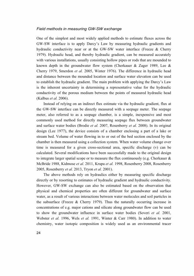
Field methods in measuring GW-SW exchange

One of the simplest and most widely applied methods to estimate fluxes across the

GW-SW interface is to apply Darcy’s Law by measuring hydraulic gradients and

hydraulic conductivity near or at the GW-SW water interface (Freeze & Cherry

1979). Hydraulic head, and thereby hydraulic gradient, can be measured accurately

with various installations, usually consisting hollow pipes or rods that are mounded to

known depth in the groundwater flow system (Cherkauer & Zager 1989, Lee &

Cherry 1979, Smerdon et al. 2005, Winter 1976). The difference in hydraulic head

and distance between the mounded location and surface water elevation can be used

to establish the hydraulic gradient. The main problem with applying the Darcy’s Law

is the inherent uncertainty in determining a representative value for the hydraulic

conductivity of the porous medium between the points of measured hydraulic head

(Kalbus et al. 2006).

Instead of relying on an indirect flux estimate via the hydraulic gradient, flux at

the GW-SW interface can be directly measured with a seepage meter. The seepage

meter, also referred to as a seepage chamber, is a simple, inexpensive and most

commonly used method for directly measuring seepage flux between groundwater

and surface water bodies (Brodie et al. 2007, Rosenberry et al. 2008). In its original

design (Lee 1977), the device consists of a chamber enclosing a part of a lake or

stream bed. Volume of water flowing in to or out of the bed section enclosed by the

chamber is then measured using a collection system. When water volume change over

time is measured for a given cross-sectional area, specific discharge (v) can be

calculated. Several modifications have been successfully made to the original design

to integrate larger spatial scope or to measure the flux continuously (e.g. Cherkauer &

McBride 1988, Kidmose et al. 2011, Krupa et al. 1998, Rosenberry 2008, Rosenberry

2005, Rosenberry et al. 2013, Tryon et al. 2001).

The above methods rely on hydraulics either by measuring specific discharge

directly or by resorting to estimates of hydraulic gradient and hydraulic conductivity.

However, GW-SW exchange can also be estimated based on the observation that

physical and chemical properties are often different for groundwater and surface

water, as a result of various interactions between water molecules and soil particles in

the subsurface (Freeze & Cherry 1979). Thus the naturally occurring increase in

concentrations of e.g. major cations and silicate along groundwater flow can be used

to show the groundwater influence in surface water bodies (Soveri et al. 2001,

Webster et al. 1996, Wels et al. 1991, Winter & Carr 1980). In addition to water

chemistry, water isotopic composition is widely used as an environmental tracer

25

(Clark & Fritz 1997, Gat 1996). Data on environmental tracers, chemical or isotopic,

can be used qualitatively to increase conceptual process understanding of the

exchange. They are also suitable for quantitative estimates of groundwater inflow via

mass balance and mixing analysis (Jones et al. 2006, Krabbenhoft et al. 1990b,

Laudon & Slaymaker 1997, Rozanski et al. 2001).

In addition to tracers analysed in water samples, heat provides a good

environmental tracer, as there is often a marked temperature difference between GW

and SW (Anderson 2005). Temperature is easy and inexpensive to measure, and the

physical basis of energy transport is well established (Kalbus et al. 2006). Therefore

use of the tracer has generated a multitude of applications spanning a range of

spatially detailed temperature profiling (Anibas et al. 2011, Brookfield et al. 2009,

Conant 2004, Jensen & Engesgaard 2011, Sebok et al. 2013) to areal thermal imaging

using aircraft and satellites (Handcock et al. 2006, Mallast et al. 2013, Rundquist et al. 1985). Differences in temperature can be used to establish rate of GW-SW

exchange and spatial occurrence of the exchange.

Numerical modelling

Since early stages, analytical and numerical solutions to groundwater flow equations

have played a key role in developing process understanding and formulating new

hypotheses to be tested in the field of GW-SW interaction studies. Early studies on

groundwater-lake interactions, many of them conducted by T.C Winter, commonly

focused on two-dimensional (2-D) cross-sections with simple geometries and

geological settings due to computational limitations (Winter 1976, Winter 1981,

Winter & Pfannkuch 1984). Even though modelling (and research) communities

were, and still largely are, divided into groundwater and surface water hydrologists,

already Freeze and Harlan (1969) outlined a blueprint for a physically-based

hydrological model which could eventually combine the groundwater and surface

water domains. Later, with the advances in computational technology, the simulation

problems for GW-SW interactions have increased notably in size and complexity

(Hunt et al. 2003, Sophocleous 2002), with rapid ongoing development to fulfil the

concept of Freeze and Harlan (Maxwell et al. 2014).

The majority of GW-SW interaction field studies involving numerical modelling

are performed within the context of spatially distributed hydrological models. In these

models, fully saturated subsurface flow is solved using spatially (and sometimes

temporally) discretised partial differential equations based on Eq. (1), which can be

extended to consider variably saturated conditions by modifying it to include the

26

Richards equation (Richards 1931). Surface water features in the models are

commonly treated as: 1) Model boundary conditions with only one-way water

exchange (Ataie-Ashtiani et al. 1999, Okkonen & Kløve 2011); 2) discrete features

with mass balance and linear water exchange with the subsurface system (Anderson

& Cheng 1993, McDonald & Harbaugh 1988, Prudic et al. 2004); or 3) partial

differential equations, most commonly the Saint-Venant equation, simulating spatially

distributed surface water flow (Maxwell et al. 2009, Panday & Huyakorn 2004).

A fundamental concept to note from the model concepts above is that the water

flow (and/or storage) in the GW and SW domains is expressed with different

mathematical formulations. Therefore the GW and SW domains must communicate in

a way which ensures conservation of mass and continuity of momentum at the model

interface (Furman 2008). The modelling community refers to this exchange of

information as model coupling, which is necessary for all models simulating GW-SW

exchange. However, the physical conceptualisation and numerical implementation of

model coupling varies between applications. Regardless of the approach, the GW-SW

interaction is simulated when water is exchanged between the domains.

HydroGeoSphere (HGS), which was used to simulate GW-SW interactions in

this thesis, is an example of a state-of-the-art, fully integrated surface-subsurface

model (Aquanty 2013). HGS uses a controlled volume finite element approach and is

capable of simulating the interconnected flow processes of subsurface and surface

water. The fully integrated approach allows water input as rainfall and snowmelt to be

partitioned into different components (surface or overland flow, evaporation,

infiltration to unsaturated soil or directly to groundwater) in a physically-based

fashion. Both surface and subsurface (saturated and unsaturated) flow regimes are

solved simultaneously at each time step, allowing water to be exchanged naturally

between the domains. Surface flow is solved with a 2-D diffusion-wave

approximation of the Saint-Venant equation and saturated/unsaturated subsurface

flow with the Richard’s equation. An integrated evapotranspiration (ET) module is

used to simulate actual ET from surficial soil layers based on potential ET time series

and soil moisture conditions. HGS has proven to be versatile and high performing in

simulating hydrological responses of systems ranging from metres to catchment and

continental spatial scale (Brookfield et al. 2009, Brunner & Simmons 2012,

Goderniaux et al. 2009, Lemieux et al. 2008, Sudicky et al. 2010). It has been used as

a reference code in simulating GW-SW interactions (Brunner et al. 2010). Even

though benchmark testing of HGS and other surface-subsurface codes has only just

started (Maxwell et al. 2014), the main conclusion so far is that the models are

27

capable of successfully reproducing the main hydrological processes in both surface

and subsurface flow.

28

29

3 Study site: Rokua esker aquifer

3.1 Hydrogeological characteristics

Esker aquifers are abundant in the Fenno-Scandinavian shield and are common in

other regions covered by the last glaciation (Svendsen et al. 2004). Eskers are

permeable, unconfined sand and gravel aquifers associated with deglaciation

(Banerjee 1975). Rivers of melting ice deposited sandy sediments in the river channel

under the ice sheet. A gravel core is usually found in the central part of esker aquifers

in the direction of glacier withdrawal, as the first phase of the glacifluvial sediment is

stratified in a high velocity meltwater flow (Mälkki 1999).

The Rokua esker aquifer is part of a long esker ridge stretching inland from the

North Ostrobothnian coast (Aartolahti 1973). The deposited overburden of

glaciofluvial origin consists of fine and medium sand sediments, mainly of quartz,

originally eroded from sedimentary rock of the Muhos formation (Aartolahti 1973,

Pajunen 1995). Rokua has rolling terrain because of kettle-holes, wave action and

aeolian dunes. The thickness of the sand deposits varies from 30 m to more than 100

m above the bedrock (Fig. 2). The sandy aquifer is underlain by crystalline bedrock

consisting mainly of igneous migmatite gneiss and granite (Aartolahti 1973).

Hydrologically, the Rokua esker aquifer is a very complex, unconfined aquifer

system with lakes and streams in the aquifer recharge area and groundwater-fed

springs and streams in the groundwater discharge area (Figs. 1 and 3). The most

important landscape feature as regards the work in this thesis is kettle-holes, which

formed during deglaciation from large blocks of ice encased within the sand deposits.

When the ice later melted, a depression was left in the landscape (Mälkki 1999). The

size of these kettle-holes at Rokua varies widely, with their depth ranging from 1–2 m

to 40 m and their diameter from some 10 m to 1.5 km long by 0.4 km wide

(Aartolahti 1973). The majority of the kettle-holes are dry, but approximately 90 lakes

or ponds with surface area ranging from 0.02 to 165 ha are located in the area.

Eskers consist of permeable sandy soils and gravels and therefore surface runoff

is usually minor. Instead, water from subsurface flow ponds in landscape depressions

such as kettle-holes. Kettle-hole lakes are usually embedded in the aquifer and their

water level and water chemistry are highly dependent on the groundwater system

(Winter et al. 1998). In addition to the physical characteristics of the lakes,

groundwater exchange affects lake ecosystems by providing nutrients, inorganic ions

and a stable water temperature (Hayashi & Rosenberry 2002).

30

Fig. 2. Conceptual model of aquifer geology as used in Paper IV for the porous media

domain. Yellow represents sand soil layers and green peat soil layers blanketing the

sandy aquifer in the discharge area. Red areas represent lake bed sediments. Vertical

exaggeration is 25 times the horizontal in all three meshes.

The groundwater discharge zone at Rokua is extensively covered by peatlands (Fig.

2), which started to form between littoral deposits of different phases of the Baltic Sea

after the glacial retreat, around 8000 years ago (Pajunen 1995). Peat is an organic soil

31

type characterised by high water content and low hydraulic conductivity (approx.

10-7–10-9 m s-1), especially in the humified catotelm layer in deep parts of the peat soil

profile (Päivänen 1973, Price 1992, Ronkanen & Kløve 2005, Silins & Rothwell

1998). However, double porosity, where preferential ‘pipe-like’ flow channels are

found in the peat matrix, can introduce a bypass route for water flow (Holden & Burt

2002, Ours et al. 1997). The majority of the Rokua peatlands were drained during the

1950s to 1980s by excavating open channel ditches to improve conditions for forest

growth.

Problems with varying lake water levels and eutrophic water quality

The geological and ecological uniqueness of the Rokua esker area is widely

acknowledged. Rokua was recently granted membership of the UNESCO GeoPark

Network and it is also part of the Finnish nature reserve network, since part of the

area is protected as a Finnish National Park (Fig. 4). Some ecosystems in the area are

protected by Natura 2000 (Metsähallitus 2008). Most of Rokua’s kettle-hole lakes and

ponds are of high ecological and recreational value because of their crystal clear

waters (Anttila & Heikkinen 2007). The lakes are widely used for recreational

activities such as fishing, swimming and scuba diving, and many of the lake shores

are populated with holiday homes and hotels.

Kettle-hole lakes in the Rokua esker aquifer are affected by two problems: 1)

Periodically declining water level in closed basin lakes (seepage lakes); and 2)

eutrophication of lakes with a surface water outlet (drainage lakes). The periodic

decline in lake water level, especially after a dry period at the beginning of the 2000s,

has raised concerns about the future of the lakes (Anttila & Heikkinen 2007). At this

point, several factors have been suggested as the reason for the decline. Land use in

the surrounding peatlands is suspected to be one of the main reasons, but more

scientific research is needed to understand the magnitude of different factors

contributing to lake level variability (Koundouri et al. 2012). Water quality in the

closed basin lakes is optimal for recreational use, but a permanent lake water level

decline would be disadvantageous for both the ecological and recreational values of

the Rokua area.

The lakes that are suffering from eutrophic conditions, manifested in poor water

quality (high phosphorus concentrations and occasional oxygen depletion) and algae

blooms (Väisänen et al. 2007), are different from those in which water levels are

periodically declining. Nutrient loading from anthropogenic sources can be

considered to be a minor nutrient source for both oligotrophic and eutrophic lakes.

32

The only obvious difference between the two lake types is surface water outlets,

which exist only in the eutrophic chain of lakes. However, previous studies have not

explained why some lakes in the Rokua area are distinctly more eutrophic than others,

despite being located in similar hydrogeological settings.

3.2 Data collection network

The data presented in this section are common to Papers I-IV. The majority of the

collected data refer to geological structure, climate variables, groundwater and

lake level recording and stream flow monitoring.

33

Fig. 3. Monitoring network for lake and groundwater levels, stream flow and climate

stations. The map shows the model boundaries used in Paper IV and the study site

locations for Papers I and II.

34

Land use

Land use in the Rokua aquifer and the surroundings consists mostly of forests

used for commercial forestry activities (Fig. 4). Some agricultural and peat

production areas are present outside the groundwater recharge area. Small-scale

anthropogenic developments, such as second homes, recreation facilities and

paved roads, have been constructed around kettle-hole lakes. Water extraction

from four intake stations in the aquifer was in total below 500 m3/d and has been

concluded to have minimal effects on aquifer water storage.

Fig. 4. The main land coverage types in the Rokua esker area. Forest land dominates,

with most of that outside the natural conservation areas being used for commercial

forestry (National Land Survey of Finland 2009).

Geological data

Rokua has been geologically surveyed with partially penetrating borehole drillings in

previous studies, but to a maximum depth of 20–30 m and without any bedrock

confirmation (Heikkinen & Väisänen 2007, Tuomikoski 1987). From 2008 to 2010,

the University of Oulu and Geological Survey of Finland mapped the Rokua esker

geology with 150 km of ground-penetrating radar line and 5 km of seismic

35

refraction/reflection measurement line (Rossi et al. 2014). These surveys revealed

fine and medium sand in the esker area, with deposit thicknesses of over 80 m above

the bedrock. Borehole logs of soil type from earlier studies characterised the soil type

mainly as medium, fine or silty sand throughout the model domain, with some local

loam lenses and gravel deposits (Aartolahti 1973, Heikkinen & Väisänen 2007,

Tuomikoski 1987). However, detailed information on soil hydraulic properties was

not available. The existing borehole logs were supplemented with additional borehole

drillings, both partially and fully penetrating, during the course of this thesis work

(Fig. 3 and Appendix 1). Bedrock surface was identified from geophysical data and

fully penetrating borehole drillings with bedrock confirmation, and a full bedrock

surface was interpolated using the points of observed bedrock.

Particle size distribution was determined for 37 soil samples taken from eight

boreholes of various depths (Appendix 1, Fig. 3, Fig. 5). Particle size distribution data

were employed to calculate the range of saturated hydraulic conductivity for the

samples, using empirical equations by Hazen, Kozeny-Carman, Breyer, Slitcher and

Terzaghi (Freeze & Cherry 1979, Odong 2007). Soil sample hydraulic conductivities

were plotted as a function of sampling depth (below ground surface and above sea

level; Fig. 5). The samples were mainly characterised as fine or medium sand,

similarly to previous borehole logs reported in Heikkinen and Väisänen (2007) and

Tuomikoski (1987). In borehole G14 (see Fig. 3), a gravel deposit was found in the

bottom of the borehole. Coarse material was also found in the eastern parts of Rokua,

near Lake Oulujärvi, in earlier surveys, but besides these observations no continuous

gravel was found based on data from the other boreholes or any of the geophysical

measurements. Four soil samples consisted of finer sediments with order of

magnitude lower K values. On combining the available data from prior borehole logs

and the geophysics and drillings performed, there was no evidence of different

stratigraphical layers, which could have been used to assign different permeability to

soil layers in a scale relevant for the models used in Papers III and IV.

36

Fig. 5. Hydraulic conductivity (K) values calculated from the soil sample particle size

distributions. Plots show (left) the estimated K values for all samples (5 calculations

per sample), (centre) the geometric mean K for each sample as a function of sampling

depth below the ground surface, and (right) the geometric mean K for each sample as

a function of sampling depth above sea level. The dashed line ‘K limits’ indicates the

range of soil hydraulic conductivity (1.99 10-5–1.47 10-3 m s-1) used in Papers III and IV.

Nine samples taken from borehole G10 were used to estimate pressure-saturation data

from parameterisation of the Brooks and Corey equation (Paper III) and van

Genuchten equation (Paper IV) (Fig. 6).

37

Fig. 6. Soil sample pressure-saturation data for sandy soil and parameterisation of the

soil pressure-saturation relationship used in Papers III and IV.

The soil data were used to define ranges for sand hydraulic conductivity in Papers III

and IV. In Paper III, the range 1.99 10-5–1.47 10-3 m s-1 was selected to cover the

minimum and maximum hydraulic conductivities based on the boreholes in the

recharge area (excluding G18 and G19) and within the unsaturated layer thickness

(sampling depth <50 m, excluding deep samples in G14). This range is in line with

typical hydraulic conductivity values for medium, fine and silty sand (Freeze &

Cherry 1979). The range was considered to reasonably represent the typical hydraulic

conductivity range in the study area for both of the modelling studies.

The Geological Survey of Finland has mapped peat thickness in parts of the study

area with peat cores (n = 4000) through the peat layer (Häikiö 2008, Pajunen 2009).

The peat thickness varies from zero to over 5 m in the aquifer discharge zone, with an

average thickness of 1.4 m. In the present work, peat hydraulic conductivity was

measured for the peatland catchment study site (S13 in Fig. 3) with a direct-push

piezometer with a falling head (Hvorselv 1951). The measurements verified the

expected low hydraulic conductivity towards the bottom layer of the peat, with a K

values of 10-5 m s-1 at a depth of 20 cm and 10-9 m s-1 at a depth of 200 cm.

An organic gyttja layer covers lake bottoms in the area and is generally known to

affect groundwater inflow to lakes (Kidmose et al. 2013, Smerdon et al. 2007, Virdi et al. 2013). This lakebed gyttja in Rokua has its origins in peat accumulated in the

bottom of ancient kettle-holes, which were later submerged and turned into lakes and

38

ponds as a result of rising groundwater level (Pajunen 1995). The extent of the gyttja

layer was studied with ground-penetrating radar at site L3, by using the equipment on

top of lake ice cover. The gyttja was absent in the immediate vicinity of the shoreline,

but in the middle of the lake the gyttja layer reached a thickness of 5 m. A similar

structure of the bottom cover, with sand near the shoreline and gyttja in the centre, has

been observed on dives in several of the area’s lakes. Field analysis of the gyttja core

showed that it contained highly decomposed organic matter with increasing mineral

soil content towards the bottom.

Climate data

The climate at the Rokua aquifer is characterised by precipitation exceeding

evaporation on an annual basis. Mean annual values (and standard deviations) during

1960–2010 were 591 mm (91 mm) for precipitation and 426 mm (26 mm) for FAO

reference evapotranspiration calculated according to Allen et al. (1998). Another

important feature of the climate is annually recurring winter periods when most

precipitation accumulates as snow. Mean annual temperature for the period 1960–

2010 was -0.7 °C (1.1 °C).

Meteorological data were mainly obtained from two sources; the Finnish

Meteorological Institute (FMI), and measurements made with a climate station

established during the project (see Fig. 3). Other databases were also utilised to some

extent, for details see Appendix 2. Data obtained from FMI had been collected

according to the Institute’s standard practices and were supplied as time series from

FMI databases. Because long historical time series of data were available only from

FMI, climate data records from Rokua climate station were used to verify the

applicability of FMI data for study site conditions.

Monitoring of lake and groundwater levels and stream discharge

Data on groundwater and lake levels were collected with manual measurements and

automated dataloggers (Solinst Levellogger Gold). The Centre for Economic

Development, Transport and the Environment (ELY Centre) started the first intensive

water level measurement campaign by installing groundwater boreholes and lake

level scales in the area for manual water level recording (Anttila & Heikkinen 2007).

The earliest data available are from 2004, with increasing temporal resolution and

spatial scope since 2007. The automated dataloggers used in the present thesis were

installed during 2008–2010 in the boreholes indicated in Appendix 1. Stilling wells

39

were installed in selected lakes to ensure high quality of lake level data. Groundwater

and lake levels were recorded with hourly resolution and the quality of the automated

measurements was verified with manual level measurements several times per year.

The outflow from the aquifer was monitored by measuring stream discharge in

the aquifer recharge and discharge area (Fig. 3). The flow was measured by

determining the flow velocity [m s-1] at different points of stream cross-section using

a portable flow meter (Mini Air 20) and calculating the outflow [m3 s-1] with respect

to the cross-sectional surface area. All measurement locations were surveyed within

2-3 days in a given measurement round. Frequency of measurements was

approximately every six weeks during May 2009–July 2011 and every three months

from August 2011 to October 2012.

40

41

4 Materials and methods

4.1 Field methods to study GW-SW interactions

4.1.1 Seepage meter measurements (I)

Seepage meter measurements were performed in lake L3 in order to: 1) Verify the

interaction between the lake and the aquifer; 2) determine the spatial distribution of

lake seepage rates; 3) study temporal variations in seepage rate within specific

locations; and 4) compare the temporal variations in lake seepage and changes in lake

and groundwater levels and determine whether changes in levels were reflected in

lake seepage rates. The seepage meters constructed in Paper I resembled the design

introduced by Lee (1977). The equipment consisted of a 208-L steel drum barrel

(diameter 57 cm) with a cut-off end, a plastic bag and a smooth 20 cm connection

hose between the bag and the chamber (Fig. 7) A total of six seepage meters, all

identical in design and components, were used in Paper I. Most common sources of

error occurring in seepage meter studies according to Rosenberry et al. (2008) were

acknowledged in both seepage meter design and in carrying out the measurements

(for full details see Paper I).

42

Fig. 7. Seepage meter in operation in Lake Ahveroinen (L3). The chamber was pushed

into the sandy lake bed sediment and water flowed into the plastic bag through the

connection hose. Picture by Riku Eskelinen.

43

Fig. 8. Hydrological monitoring locations in Lake Ahveroinen (L3). Spatial distribution

of seepage meter measurements for the two years is represented as crosses of

different colours and the locations used to study temporal seepage variability during

2010 are named (001–006). Reprinted with permission from Elsevier (Paper I).

The first set of seepage meter measurements focused on determining the spatial

distribution of seepage direction and rate at site L3 (Lake Ahveroinen). The spatial

distribution of seepage rates around the lake in 2009 was determined at 16 locations

(Fig. 8). The second set of seepage meter measurements studied temporal variations

in seepage rate. Eight seepage meter measurements were made at six locations (Fig.

8), at approximately 3-week intervals. A full description of the measurements is given

in Paper I.

Statistical analysis of seepage meter measurements and hydrological observations

In order to detect whether changes in seepage rate co-varied with changes in the

surrounding hydrogeology, the correlation between seepage velocities and lake and

44

groundwater levels was analysed on the date of seepage measurements. In order to

acknowledge the linear relationship between hydraulic gradient and groundwater flow

velocity (in this case seepage velocity), Pearson correlation coefficient expressing

linear correlation was used in the analysis and correlations with p-values below 0.05

were considered to demonstrate a strong correlation. It should be noted that reported

p-values for correlations between seepage measurements and hydrological

observations are prone to type I errors, because the seepage measurements themselves

are correlated and thus the variables are not independent. However, the aim in the

present work was to examine whether the seepage rates respond to different parts of

the hydrogeological system and for that purpose p-values provided a convenient cut-

off point to classify locations into correlated and non-correlated, even though the

statistical validity of significance was compromised.

4.1.2 Hydraulic measurements in the peatland drainage network (II)

Groundwater discharge into drained peatland was studied in the upper catchment area

of the Siirasoja stream (S13, see Fig. 3). S13 had one of the highest baseflow runoff

values recorded in the Rokua study site catchment and therefore a strong groundwater

influence on the drainage ditch network was suspected in the area. The study site (1.5

km2) was divided into four subcatchments A–D (Fig. 9) to study the spatial variability

in groundwater discharge. At the southern side of the peatland, where the soil type

transitions from peat to sand, the sandy esker formation rises with a steep 30% slope

(Fig. 10).

45

Fig. 9. Diagram of the Siirasoja stream catchment study site (S13) showing its four

subcatchments A–D, groundwater monitoring wells (G10, G11), piezometers (G12a &

b), stream water sampling points, and peat thickness measurement points. Reprinted

with permission from Elsevier (Paper II).

46

Fig. 10. Cross-section along the monitoring well installation line in the Siirasoja

stream catchment (S13) (with 10:1 vertical exaggeration) showing the thickness of

peat and sand deposits and the groundwater monitoring well installation set-ups.

Reprinted with permission from Elsevier (Paper II).

The drainage ditches in the subcatchments were mapped for water flow rate and

presence of spring-like groundwater exfiltration points in situ during low-flow season

in July 2009. Point discharges were first visually identified and then confirmed with

water temperature measurements before and after the observed point discharge.

Groundwater during the monitoring period was colder than rain-fed surface water,

and the temperature difference was used as a tracer for groundwater inflow. When no

point discharge was observed but the flow rate in the drainage ditch was increased

and water temperature was low, ditches were considered to receive groundwater

seepage. Groundwater level in both the sand aquifer and peat soil (Figs. 9 and 10) was

recorded with automated levelloggers (see Section 3.2) to establish the hydraulic

gradients at the site.

47

4.1.3 Environmental tracers (I & II)

The environmental tracers calcium (Ca2+), silica (SiO2) and the ecologically

significant nutrient phosphate (PO3-4) were used to study GW-SW interactions at

aquifer scale (Paper I) and surface water body scale (Papers I and II) in the Rokua

aquifer. The environmental tracers were used to look for similarities and/or

differences in groundwater and surface water chemical composition throughout the

aquifer. Of the selected tracers, phosphate is not a suitable environmental tracer as

such because of its active biological uptake and tendency to be adsorbed on soil

minerals and organic matter. However, below the organic-rich and biologically active

soil zone, the amount of phosphorus in groundwater is mainly controlled by the

solubility of sparingly soluble phosphate-bearing minerals (Freeze & Cherry 1979). In

this respect groundwater inflow can provide a phosphate source to lakes (Devito et al. 2000, Kidmose et al. 2013, Shaw et al. 1990).

Sampling strategies for environmental tracers

Water samples were taken in all relevant hydrological compartments of the study

aquifer (10 piezometers, 13 lakes, 9 streams, 1 snowfall) at a total of 33 locations

(Fig. 3, Appendix 1). Details about the sampling procedure and analysis methods are

given in Paper I. On aquifer scale, tracer concentrations were statistically compared

against the altitude of the sampling location using the rank-based Kendall correlation

analysis. The underlying assumption was that water sampled at lower altitudes had

travelled along a longer flow path in the subsurface and would therefore be richer in

tracers indicating mineral weathering and dissolution (Kenoyer & Bowser 1992,

Webster et al. 1996, Winter & Carr 1980, Winter 1999). In addition, phosphate

concentrations were compared with calcium and silica concentrations in order to

determine whether the phosphate concentrations in different parts of the study site

were related environmental tracers known to reflect the length of the subsurface flow

path. For descriptive statistics, the median was selected as the measurement of central

location and the interquantile range as the measurement of spread because of

observed non-normal distribution, especially of phosphate samples.

On the scale of a single lake, tracer concentrations of a surface water body (L3)

and the adjacent groundwater were examined. In this case the aim was to look for

differences in lake water and groundwater tracer concentrations and from that

estimate the magnitude of groundwater influence and water flow directions. Sampling

48

was performed in piezometers near the lake (Fig. 8, Appendix 1) as part of the aquifer

sampling.

In the drained peatland at the Siirasoja stream study site (Figs. 9 and 10),

environmental tracers were used to characterise the groundwater flow path in the

aquifer beneath the peat layer and to estimate the contribution of groundwater

exfiltration to stream flow. Samples were taken during the field study campaign in

June 2010. Water was sampled from stream water (sample points 1–4), groundwater

wells and piezometers, and precipitation (Fig. 9, Appendix 1). In the drained peatland

area, the samples were also analysed for pH and electrical conductivity (EC) to

supplement the other analyses.

4.1.4 Airborne thermal infrared imaging (IV)

Water surface temperature was used as a tracer to identify locations where

groundwater discharges into lakes. Airborne thermal infrared imaging (TIR) for the

lakes was conducted from a helicopter on 5 August 2013, because at around this time

of year the temperature difference between the lake water (~20 °C) and the

groundwater (~4.5 °C) is highest. Imaging was performed using the Flir Thermacam

P-60 thermal camera with 320 x 240 pixel sensor resolution and an aperture of 24°. It

covered the electromagnetic spectrum from 7.5 to 13 µm. The imaging was carried

out from 150 m above the lake surface, making the pixel size approximately 15 cm x

15 cm. Temperature gradients were identified visually from the TIR images. Lakes

were imaged only for their shoreline and the central areas of the larger lakes were

omitted. Theoretically the groundwater inseepage rates should be greatest near the

shoreline, close to the ‘break in slope’ the surface water body exerts on the

groundwater level (Freeze & Cherry 1979), a phenomenon previously shown in field

and modelling studies (Barwell 1981, Cherkauer & Nader 1989, Rosenberry &

LaBaugh 2008). Another reason to focus on lake shorelines was that the method

records the skin temperature of the water surface and therefore groundwater discharge

deeper in a lake is likely to be undetectable as colder groundwater is mixed within the

water column (Torgersen et al. 2001). When a temperature pattern on the lake

shoreline suggested anomalously cold temperature (Fig. 11), the spatial coordinates

were saved in ArcGIS software (ESRI 2011).

49

Fig. 11. Example of data obtained from air-borne thermal imaging (TIR) comprising

(left) screenshots from a normal video camera and (right) thermal infrared images at

the same location showing (upper image) an example of diffuse inflow (large purple

area) and (lower image) focused inflow (small blue area). The maximum temperature

difference is ~5 °C in the upper image and ~10 °C in the lower image. The colour

schemes vary between the pictures. Pictures by Pekka M. Rossi.

50

4.2 Simulations for spatially and temporally distributed recharge (III)

Detailed information about the groundwater recharge in Rokua esker aquifer was

acquired by a numerical modelling study (Paper III). This sought to expand the

application of physically-based 1-D unsaturated water flow modelling (Assefa &

Woodbury 2013, Hunt et al. 2008, Jyrkama et al. 2002, Keese et al. 2005, Okkonen &

Kløve 2011) to simulate spatial and temporal variations in groundwater recharge,

while taking into account detailed site-specific information on vegetation (pine,

lichen), unsaturated soil thickness, cold climate and simulation parameter uncertainty.

CoupModel (Jansson & Karlberg 2004) was used in simulations because of its ability

to represent the full soil-plant-atmosphere continuum adequately and to include snow

processes in the simulations (Okkonen & Kløve 2011). The modelling set-up

developed in Paper III uses spatially detailed information on tree canopy properties

and concentrates on simulating different components of evapotranspiration.

Furthermore, it considers the effect that forestry land use has on vegetation

parameters and how this is reflected in groundwater recharge. The simulation

approach takes into account the variability in the unsaturated zone thickness

throughout the model domain. Parameter uncertainty, often neglected in recharge

simulations, is considered by using multiple random Monte Carlo simulation runs in

the process of distributing the 1-D simulations spatially. The overall aim of Paper III

was to provide novel information on groundwater recharge rates and factors

contributing to the amount, timing and uncertainty of groundwater recharge in

unconfined sandy eskers aquifers.

4.2.1 Vegetation and unsaturated zone parameterisation

Forestry inventory data from the Finnish Forest Administration (Metsähallitus,

MH) and Finnish Forest Centre (Metsäkeskus, MK) were used to estimate leaf

area index (LAI) for the Rokua esker groundwater recharge area. The available

data consisted of 2786 individual plots covering an area of 52.4 km2 (62.4% of

the model domain). The forestry inventories, performed mainly during 2000–

2011, showed that Scots pine (Pinus sylvestris) is the dominant tree in the model

area (94.2% of plots). For details of LAI calculation, see Paper III.

The calculated spatially distributed information on LAI (Fig. 12) was used to

obtain an estimate of how different land use management options, already actively in

operation in the area, could potentially affect groundwater recharge. Clear-cutting is

51

an intensive land use form in which the entire tree stand is removed, and it is carried

out in some parts of the study area. The first scenario simulated the impact of clear-

cutting by not resorting to the estimated LAI pattern at the site, but by using an LAI

value of 0–0.2 for the whole simulated area. In the second scenario, which was the

opposite of clear-cutting, the mature stand was assumed to have high LAI values of

3.2–3.5 found at the study site and reported in the literature (Koivusalo et al. 2008,

Rautiainen et al. 2012, Vincke & Thiry 2008, Wang et al. 2004).

Fig. 12. Spatial distribution of leaf area index (LAI) and a 20 m x 20 m cell-based

histogram of LAI values. In areas where forestry inventory data were lacking, a

weighted average value of 1.25 was used in simulations. CC BY 3.0 (Paper III).

An organic lichen layer covers much of the sandy soil at the Rokua study site

(Kumpula et al. 2000), so a lichen layer was included in soil evaporation (SE)

calculations. Lichen vegetation has the potential to affect SE by influencing the

evaporation resistance of soil and by intercepting rainfall before it enters the mineral

soil surface (Kelliher et al. 1998). Although lichens do not transpire water, their

structural properties allow water storage in the lichen matrix and capillary water

52

uptake from the soil (Blum 1973, Larson 1979). The lichen layer also increases soil

surface roughness and thereby retards surface runoff (Rodríguez-Caballero et al. 2012).

In this thesis, water interception storage by the lichen layer was estimated from

lichen samples. The mean water retention capacity of the lichen samples was found to

be 9.85 mm (standard deviation (SD) 2.71 mm) and approximations for these values

were used in model parameterisation (Table 1). In the simulations, the lichen layer

was represented as an organic soil layer with similar Brooks and Corey (B&C)

parameterisation as for mineral soil and the B&C parameters were included in the

uncertainty analysis.

The thickness of the unsaturated layer was estimated by subtracting interpolated

groundwater level from digital elevation model (DEM) topography calculated based

on LiDAR data (National Land Survey of Finland 2012). Groundwater elevation was

estimated with the ordinary Kriging interpolation method from four types of

observations: groundwater boreholes, stages of kettle-hole lakes, elevation of

wetlands located in landscape depressions, and land surface elevation at the model

domain. Spatial distribution and details about the calculation of unsaturated layer

thickness are presented in Paper III.

4.2.2 Simulation framework

Recharge was estimated by simulating water flow through an unsaturated 1-D soil

column with the Richards equation using CoupModel (Jansson & Karlberg 2004). To

distribute the simulations spatially, the recharge area was subdivided into different

recharge zones, similarly to e.g. Jyrkämä et al. (2002). As each zone requires a unique

simulation, the number of simulation set-ups rapidly increases, leading to high

computational demand and/or laborious manual adjustment of model set-up. In the

present work, this was avoided by simulating water flow in a single unsaturated 1-D

soil column multiple times with different random parameterisations and distributing

the results spatially to model zones. Spatial coupling was done with the ArcGIS

software (ESRI 2011).

Zonation in the model was based on two variables: LAI and unsaturated zone

thickness (UZD). Both variables were spatially distributed to a grid map with 20 m x

20 m cell size, resulting in a total of 205 708 cells for the model domain. The spatially

distributed data were then divided into 15 classes for LAI and 30 classes for UZD (see

Fig. 12 for LAI). Finally, the classified LAI and UZD data were combined to a raster

53

map with 20 m x 20 m cell size, producing 449 different zones with unique

combinations of LAI and UZD values.

Simulations for the unsaturated 1-D soil profile were made for the period 1970–

2010, and before each run 10 years of data (1960–1970) were used to spin up the

model. The time variable boundary condition for water flow at the top of the column

was defined by driving climate variables and affected by sub-routines accounting for

snow processes. All water at the top of the domain was assumed to be subjected to

infiltration. Deep percolation as gravitational drainage was allowed from the soil

column base using the unit-gradient boundary condition (see e.g. Scanlon et al. 2002b). The column was vertically discretised into 60 layers with increasing layer

thickness deeper in the profile: Layer thickness was 0.1 m until 1.6 m depth (the first

layer lichen), 0.2 m between 1.6 and 3 m, 0.5 m between 3 and 10 m, 1 m between 10

and 17 m and 2 m from 17 m to the bottom of the profile (51 m).

The simulation was performed as 400 Monte Carlo runs to ensure enough model

runs would be available for each LAI range. The model was run each time with

different parameter values as specified in Table 1. The parameters for which values

were randomly varied were chosen beforehand by trial and error model runs exploring

the sensitivity of parameters with respect to cumulative recharge or

evapotranspiration. The parameter ranges were specified from field data when

possible; otherwise we resorted to literature estimates or in some cases used ± 50% of

the CoupModel default providing a typical parameter for the equation. Paper III

provides an illustrated example how the 1-D simulations were spatially distributed in

the model domain.

54

Table 1. Randomly varied parameters, related equations and parameter ranges

included in the model runs. For a full description of parameters and equations, see

Jansson and Karlberg (2004).

Parameter Part of the model

affected

Range Units Source

LAI (leaf area index) Transpiration 0…3.5 - Data, see Section 4.2.1

h (canopy height) Transpiration 5…15 m Data

ralai (increase in

aerodynamic

resistance with LAI)

Soil evaporation 25…75 - ±50%, estimate

rΨ (soil surface

resistance control)

Soil evaporation 100…300 - ±50% approximately to cover the

surface resistance reported in (Kelliher

et al. 1998)

λL (pore size

distribution index)

Soil evaporation,

lichen

0.4…1 - Estimate, to cover an easily drainable

range of pressure-saturation curves

ΨL (air entry) Soil evaporation,

lichen

1.5…20 - Estimate, to cover a easily drainable

range of pressure-saturation curves

θL (porosity) Soil evaporation,

lichen

7.5…12.5 % Data, lichen mean water retention ±SD

from samples

kmat,L (matrix saturated

hydraulic conductivity)

Soil evaporation,

lichen

5*104…5*107 mm

d-1

Estimate, high K values assumed

tWD (coef.temperature

response function)

Water uptake 10…20 - ±50%, estimate

Ψc (critical pressure

head for water uptake)

Water uptake 200…600 - ±50%, estimate

kmat,S (matrix saturated

hydraulic conductivity)

Soil profile 1.71*103…

127*103

mm

d-1

Data from soil sample particle size

analysis

kminuc (min. unsat.

hydraulic conductivity

Soil profile 1 10-4…1 10-1 mm

d-1

Estimate kmat * 10-5

λs (pore size

distribution index)

Soil profile 0.4…1 - Range to cover measured pressure-

saturation curves

Ψs (air entry) Soil profile 20…40 - Range to cover measured pressure-

saturation curves

θs (porosity) Soil profile 0.25…0.36 % Range from soil samples

θr (residual water

content)

Soil profile 0.01…0.05 % Range to cover measured pressure-

saturation curves

55

After completing the 400 CoupModel simulations for the unsaturated soil column,

each unique recharge zone (a combination of UZD and LAI class) had on average 27

recharge time series produced by different random combinations of parameters. To

propagate the variability in the 27 time series into the final areal recharge, a recharge

value was randomly selected for each time step and each recharge zone from the

ensemble of 27 (on average) and multiplied by the number of model cells belonging

to the recharge zone in question (Eq. 2). This procedure was carried out for all time

steps and then repeated a number of times (here 150 times) to ensure that all of the

simulated time series for each recharge zone were represented in the random selection

process.

, ∑ ∗ , : ∗ (2)

where Ri,j is the final sample of areal recharge [mm d-1], i is the index for simulation

time step (= 1:14975), j is the index for sample for a given time step (1:150), l is the

index for unique recharge zone, n(l) is the number of cells in a given recharge zone,

Rs is the recharge sample [mm d-1] for a given recharge zone at time step I, k is the

number of time series for a given recharge zone, Ac is the surface area of a model

raster cell (=20 m * 20 m = 400 m2), and Atot is the surface area of the total recharge

area.

The resulting R matrix has 150 time series for areal recharge produced by simulations

with different parameter realisations. The variability between the time series provides

an indication of how much the simulated recharge varies due to different model

parameter values. The method allows computationally efficient recharge simulations,

because the different recharge zones do not all have to be simulated separately.

Four different evaporation processes were considered in this thesis; soil, snow,

and lake evaporation and transpiration. In areas with unsaturated soil zones, the first

three evaporation components were estimated, along with water flow simulations,

using CoupModel. However, as 3.6% of the surface area of the study site consists of

lakes (Fig. 3), lake evaporation from free water surfaces was calculated independently

from the CoupModel simulations. Kettle-hole lakes in esker aquifers often lack

surface water inlets and outlets and are therefore an integral part of the groundwater

system (as shown in Section 5.1.1), so these lakes were considered as contributors to

total groundwater recharge. In other words, rainfall per lake surface area was treated

as an equal addition to aquifer water storage as groundwater recharge. As a

difference, lake water table is subjected to evaporation unlike the groundwater table.

56

A detailed description of calculation of evaporation components is provided in Paper

III.

The modelling method assumes that:

1. Over the long-term, the water table remains at a constant level, i.e. the

unsaturated thickness for each model cells stays the same. Monitoring data

shows water table variability of 1–2 m, with lowering and recovery of the

water table. This variability is within the accuracy of water table estimation

by interpolation, and therefore the assumption of long-term equilibrium was

acceptable for the study site.

2. Surface runoff is negligible primarily due to the permeable soil type, and also

due to lichen cover inhibiting runoff (Rodríguez-Caballero et al. 2012).

3. Only vertical flow takes place in the unsaturated soil matrix, a typical

assumption in recharge estimation techniques (Dripps & Bradbury 2010,

Jyrkama et al. 2002, Scanlon et al. 2002a).

4. The capillary fringe in the sandy soil is thin enough not to affect the water

flow before arriving at the ‘imaginary’ water table at the centre of each soil

class.

5. Uncertainties in the estimation of spatially distributed LAI and UZD values

justify the use of approximations (i.e. water flow at the UZD class range

midpoint and LAI value specified only as a range for each cell) in the cell

classification phase.

Model performance was tested by comparing the simulated recharge values with

two independent recharge estimates on local and regional scale; the water table

fluctuation (WTF) method and base flow estimation, respectively. The WTF

method is routinely used to estimate groundwater recharge because of its

simplicity and ease of use, and assumes that any rise in water level in an

unconfined aquifer is caused by recharge arriving at the water table (Healy &

Cook 2002). The WTF method was applied to six water table wells (Appendix 1).

For details about the method application, see Paper III.

The recharge estimated with the WTF method was compared with the simulated

recharge during the recorded water level rise in the well. For each well, the

cumulative sum of simulated water flow was extracted from soil profile depth

corresponding to well water table depth. As an example, the simulated recharge in

well G4 (unsaturated depth on average 14.7 m) was extracted from soil class 12,

corresponding to recharge for unsaturated thickness of 14–16 m. All 400 model runs

57

were used, providing 400 estimates of recharge for each time period of recorded water

level rise.

A regional estimate of groundwater recharge was estimated as baseflow of

streams originating at the groundwater discharge area (Fig. 3). The lowest total

outflow during 9–10 February 2010 was recorded after three months of snow cover,

when water contribution to streams from surface runoff was minimal. The minimum

outflow was considered as baseflow from the aquifer reflecting long-term

groundwater recharge in the area.

4.3 Fully integrated surface-subsurface flow modelling (IV)

In Paper IV, magnitude, temporal variability and spatial distribution of water fluxes at

the GW-SW interface were estimated using a fully integrated hydrological modelling

code HGS (Aquanty 2013). This integrated the conceptual and hydrogeological

understanding of the Rokua esker aquifer acquired in Papers I, II and III using a state-

of-the-art numerical simulator. The model results were compared with field

techniques used to estimate (1) GW-lake exchange locations with air-borne

measurement of water temperature and water sampling to estimate (2) exchange

magnitude with the stable isotope technique. Paper IV tested the ability of the fully

integrated numerical model to reproduce exchange between groundwater and surface

water in a complex unconfined aquifer system.

4.3.1 Model application to Rokua esker aquifer

Model mesh and driving data

The model domain was discretised into 6-node triangular prismatic finite elements. In

the subsurface, a total of 117 264 elements and 69 244 nodes comprised the

simulation domain in six vertical finite element layers (see Fig. 2). In the vertical

direction, the discretisation was refined near the ground surface to better represent the

variable soil moisture conditions in the evaporative zone (thickness 1 m) and the

water exchange processes between the subsurface and surface domains. In the lateral

direction, the mesh was refined near streams, lakes and the boundary of the

groundwater recharge area to focus calculation efforts on areas where subsurface-

surface exchange fluxes were expected. Details about the mesh refinement are given

in Paper IV.

58

Boundary conditions in the porous media consisted of a no-flow boundary in the

bottom of the model due to low permeability bedrock, prescribed head boundaries

defined by regional surface water bodies and a no-flow boundary in the rest of the

model domain perimeter because of bedrock outcrops and thin soil layers. Detailed

rationale on the assignment of boundary conditions is presented in Paper IV. A

critical depth boundary condition was assigned around the perimeter of the model

surface domain. The critical depth boundary condition does not constrain the flow rate

or flow depth in the surface flow domain, but allows discharge to change naturally

with respect to the calculated water depth at the stream outlet.

The model was sequentially coupled with Coup Model described in Paper III,

which provided input data for the simulations as time series of infiltration (water

arriving at the soil surface as a result of precipitation and/or snowmelt) and potential

evapotranspiration (PET) for the period 1 Oct 2000–30 Sept 2013. The data were

acquired from the groundwater recharge simulations (Section 4.2), with the addition

of extending the simulation time to provide time series until September 2013. The

simulations included calibrated routines for snow storage and snowmelt, which are

necessary for the correct timing of water input in the system. In addition to climate

data, the recharge simulations provided daily time series for groundwater recharge. In

this part of the work the recharge data were used to calculate the average recharge

over the simulation period (1 Oct 2000–30 Sept 2013) and the average recharge was

used to calibrate the soil hydraulic properties in steady state.

The model was run first in steady state as part of model calibration to match the

groundwater and lake levels and stream outflow in the system (see Section 4.3.2). The

final system state after the steady state calibration was then used as initial conditions

for a transient spin-up period. A recent study by Ajami et al. (2014) demonstrated that

the equilibration time for integrated surface-subsurface models may require from a

couple of years up to more than 20 years, especially to stabilise water storage in the

subsurface. In this thesis, a 20 year spin-up period was used to ensure the system had

reached a state where the water storages and fluxes were represented correctly at the

beginning of the actual simulation period. The spin-up was performed with infiltration

and PET data for the period 1 July 1980–30 Sept 2000 taken from the recharge

simulations (Section 4.2). The spin-up was performed only once because of the

computational burden and therefore the criterion of the spin-up performance (see e.g.

Ajami et al. 2014) was not calculated.

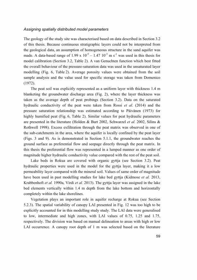
59

Assigning spatially distributed model parameters

The geology of the study site was characterised based on data described in Section 3.2

of this thesis. Because continuous stratigraphic layers could not be interpreted from

the geological data, an assumption of homogeneous structure in the sand aquifer was

made. A data-based range of 1.99 x 10-5 – 1.47 10-3 m s-1 was used in this thesis for

model calibration (Section 3.2, Table 2). A van Genuchten function which best fitted

the overall behaviour of the pressure-saturation data was used in the unsaturated layer

modelling (Fig. 6, Table 2). Average porosity values were obtained from the soil

sample analysis and the value used for specific storage was taken from Domenico

(1972).

The peat soil was explicitly represented as a uniform layer with thickness 1.4 m

blanketing the groundwater discharge area (Fig. 2), where the layer thickness was

taken as the average depth of peat probings (Section 3.2). Data on the saturated

hydraulic conductivity of the peat were taken from Rossi et al. (2014) and the

pressure saturation relationship was estimated according to Päivänen (1973) for

highly humified peat (Fig. 6, Table 2). Similar values for peat hydraulic parameters

are presented in the literature (Holden & Burt 2002, Schwarzel et al. 2002, Silins &

Rothwell 1998). Excess exfiltration through the peat matrix was observed in one of

the sub-catchments in the area, where the aquifer is locally confined by the peat layer

(Figs. 3 and 9). As is demonstrated in Section 5.1.1, the groundwater reaches the

ground surface as preferential flow and seepage directly through the peat matrix. In

this thesis the preferential flow was represented in a lumped manner as one order of

magnitude higher hydraulic conductivity value compared with the rest of the peat soil.

Lake beds in Rokua are covered with organic gyttja (see Section 3.2). Peat

hydraulic properties were used in the model for the gyttja layer, making it a low

permeability layer compared with the mineral soil. Values of same order of magnitude

have been used in past modelling studies for lake bed gyttja (Kidmose et al. 2013,

Krabbenhoft et al. 1990a, Virdi et al. 2013). The gyttja layer was assigned in the lake

bed elements vertically within 1.4 m depth from the lake bottom and horizontally

completely within the lake shorelines.

Vegetation plays an important role in aquifer recharge at Rokua (see Section

5.2.3). The spatial variability of canopy LAI presented in Fig. 12 was too high to be

explicitly accounted for in this modelling study study. The LAI data were generalised

to low, intermediate and high zones, with LAI values of 0.75, 1.25 and 1.75,

respectively. The division was based on manual delineation to areas with high or low

LAI occurrence. A canopy root depth of 1 m was selected based on the literature

60

(Kalliokoski 2011, Vincke & Thiry 2008). Pinus sylvestris roots are concentrated near

the soil surface (Helmisaari et al. 2007, Kalliokoski 2011) and an exponential

function that allocates the transpiration losses in the topmost soil layers was used to

describe the root distribution within the 1 m depth chosen. Overland flow properties

were assigned to two different domains: stream channels and forests. Manning’s n

values for the domains were taken from the literature (Jones et al. 2008).

Table 2. Model parameterisation for spatially distributed parameters that deviated

from HydroGeoSphere (HGS) model default values (Aquanty 2013).

Model Domain Parameter Value

Porous media Sand Peat

Saturated Kz [m s-1] 2*10-5 [1,2] 1*10-7 [3]

Anisotropy Kz : Kxy 1 : 2 [2] 1:1

Specific storage [1 m-1] 2 * 10-4 [4] 1 *10-1

Porosity 0.3425 [1] 0.86 [3]

Residual saturation 0.044 [1] 0.058 [3]

van Genuchten α 2.35 [1] 26.15 [3]

van Genuchten β 2.38 [1] 1.39 [3]

Minimum relative permeability 1 * 10-9 1 * 10-11

Overland flow Sand Peat Channel

Manning’s n 0.6 [5] 0.6 [5] 0.04 [5]

Rill storage height 0.1 [6] 0.1 [7] 0.001 [5]

Obstruction height 0.05 0.05 0.001 [5]

Evapotranspiration Peat Sand 1 [2] Sand 2 [2] Sand 3 [2]

LAI 1.14 0.75 1.25 1.75

Canopy storage parameter 0 0 0 0

Initial interception storage 0 0 0 0

Transpiration fitting C1 0.06 0.4 0.4 0.3

Transpiration fitting C2 0.15 -0.1 -0.1 0

Wilting point 0.06 0.06 0.06 0.06

Field capacity 0.15 0.25 0.25 0.25

Oxic limit 0.99 0.6 0.6 0.6

Anoxic limit 1.0 0.9 0.9 0.9

Evaporation lim. sat min 0.1 0.04 0.04 0.04

Evaporation lim. sat min 0.25 0.40 0.37 0.30

Root zone depth 1 1 1 1

Evaporation depth 1 1 1 1

Data sources: [1] field data, [2] calibration, [3] Päivänen (1973), [4] Domenico (1972), [5] Jones et al

(2008), [6] Paper III, [7] Frei and Fleckenstein (2014)

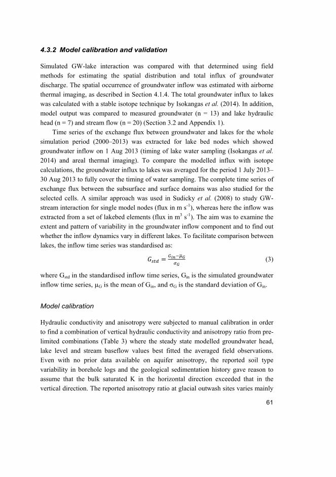
61

4.3.2 Model calibration and validation

Simulated GW-lake interaction was compared with that determined using field

methods for estimating the spatial distribution and total influx of groundwater

discharge. The spatial occurrence of groundwater inflow was estimated with airborne

thermal imaging, as described in Section 4.1.4. The total groundwater influx to lakes

was calculated with a stable isotope technique by Isokangas et al. (2014). In addition,

model output was compared to measured groundwater (n = 13) and lake hydraulic

head (n = 7) and stream flow (n = 20) (Section 3.2 and Appendix 1).

Time series of the exchange flux between groundwater and lakes for the whole

simulation period (2000–2013) was extracted for lake bed nodes which showed

groundwater inflow on 1 Aug 2013 (timing of lake water sampling (Isokangas et al. 2014) and areal thermal imaging). To compare the modelled influx with isotope

calculations, the groundwater influx to lakes was averaged for the period 1 July 2013–

30 Aug 2013 to fully cover the timing of water sampling. The complete time series of

exchange flux between the subsurface and surface domains was also studied for the

selected cells. A similar approach was used in Sudicky et al. (2008) to study GW-

stream interaction for single model nodes (flux in m s-1), whereas here the inflow was

extracted from a set of lakebed elements (flux in m3 s-1). The aim was to examine the

extent and pattern of variability in the groundwater inflow component and to find out

whether the inflow dynamics vary in different lakes. To facilitate comparison between

lakes, the inflow time series was standardised as:

(3)

where Gstd in the standardised inflow time series, Gin is the simulated groundwater

inflow time series, µG is the mean of Gin, and σG is the standard deviation of Gin.

Model calibration

Hydraulic conductivity and anisotropy were subjected to manual calibration in order

to find a combination of vertical hydraulic conductivity and anisotropy ratio from pre-

limited combinations (Table 3) where the steady state modelled groundwater head,

lake level and stream baseflow values best fitted the averaged field observations.

Even with no prior data available on aquifer anisotropy, the reported soil type

variability in borehole logs and the geological sedimentation history gave reason to

assume that the bulk saturated K in the horizontal direction exceeded that in the

vertical direction. The reported anisotropy ratio at glacial outwash sites varies mainly

62

from 1:2 to 1:10 (Hunt et al. 2013, Krabbenhoft et al. 1990a, Smerdon et al. 2007,

Sudicky et al. 2010) and these values were selected for calibration. Recharge was

applied only in the aquifer recharge area because of the complex recharge discharge

pattern expected in the discharge area covered with peat. The water seeping to the

streams from the aquifer was thus considered to represent the simulated steady-state

stream baseflow, and peat layer contribution to baseflow was assumed to be minor.

Table 3. Saturated hydraulic conductivity and anisotropy ratio (Kz: Kx and Ky) values

used in model calibration.

1 2 3 4 5 6 7 8 9

K [m s-1] 2 10-4 2 10-4 2 10-4 6.5 10-5 6.5 10-5 6.5 10-5 2 10-5 2 10-5 2 10-5

aniso.

ratio

1:2 1:5 1:10 1:2 1:5 1:10 1:2 1:5 1:10

The steady state recharge values in the model calibration phase were based on the

recharge estimation method presented in Section 4.2. Spatially distributed constant

recharge values (Table 4) were applied to zones with different LAI. Because the

recharge calculations did not provide recharge for unique LAI zones delineated in this

thesis, the recharge in different zones was related to the ET in the recharge

simulations (Table 4). After calibration, the model was run in transient mode with

daily data for water input and PET. To maintain the consistency between steady state

and transient simulations, the empirical ET parameters for each LAI zone in HGS

(Table 3) were calibrated to match the total ET amount and to approximately

reproduce the daily ET dynamics. With this procedure, the magnitude of both

recharge (steady state calibration) and ET (transient runs) in this thesis was related to

that in prior simulations for groundwater recharge. The best match between the two

simulations for total evapotranspiration (Table 4) was found with ET parameters for a

given LAI value presented in Table 2.

Table 4. Mean areal evapotranspiration (ET) and recharge for zones with different leaf

area index (LAI) values. For areas with LAI 0.75 and 1.75, recharge was calculated by

multiplying the recharge for areas with LAI = 1.25 by 402.0 [mm a-1] with ET ratios

199.9/234.0 and 255.4/234.0, respectively.

LAI = 0.75 LAI = 1.25 LAI = 1.75

Paper III

Recharge [mm a-1]

470.6 402.0 368.3

Paper III ET [mm a-1] 199.9 234.0 255.4

Paper IV ET [mm a-1] 202.7 227.7 252.7

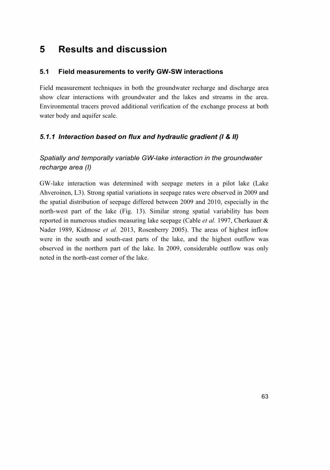
63

5 Results and discussion

5.1 Field measurements to verify GW-SW interactions

Field measurement techniques in both the groundwater recharge and discharge area

show clear interactions with groundwater and the lakes and streams in the area.

Environmental tracers proved additional verification of the exchange process at both

water body and aquifer scale.

5.1.1 Interaction based on flux and hydraulic gradient (I & II)

Spatially and temporally variable GW-lake interaction in the groundwater

recharge area (I)

GW-lake interaction was determined with seepage meters in a pilot lake (Lake

Ahveroinen, L3). Strong spatial variations in seepage rates were observed in 2009 and

the spatial distribution of seepage differed between 2009 and 2010, especially in the

north-west part of the lake (Fig. 13). Similar strong spatial variability has been

reported in numerous studies measuring lake seepage (Cable et al. 1997, Cherkauer &

Nader 1989, Kidmose et al. 2013, Rosenberry 2005). The areas of highest inflow

were in the south and south-east parts of the lake, and the highest outflow was

observed in the northern part of the lake. In 2009, considerable outflow was only

noted in the north-east corner of the lake.

64

Fig. 13. Spatial variations in seepage (µm s-1) in two consecutive years. Seepage rates

are presented as circles, with relative size and colour showing the rate and direction

of seepage, respectively. For the year 2010, the average value from the eight

measurements performed is shown. Reprinted with permission from Elsevier (Paper I).

In 2010, temporal changes in seepage rates were observed at every observation point,

but the temporal variation in seepage rates was low (Fig. 14). This variation, despite

being small, cannot be attributed to measurement error or random natural variability

because of the high observed covariation between seepage rates at four out of six

measurement points. This demonstrates the capability and accuracy of the seepage

meter measurement method to distinguish small changes in the groundwater flow

environment as long as the meter chambers are not removed between measurements.

65

Fig. 14. Temporal variations in seepage (µm s-1) during 2010 for each seepage

measurement location in Lake Ahveroinen (L3). Positive values correspond to

inseepage, µ denotes the mean and σ the standard deviation of the measurements.

Reprinted with permission from Elsevier (Paper I).

Variations in the seepage rates for the measurement locations were correlated with

different parts of the hydrogeological system (Table 5). Locations 001 and 006, where

the highest outseepage rates were measured, correlated with piezometers G20 and G6

in the direction of outseepage. Location 004, with low seepage rate, was correlated

with lake stage and piezometer G21 where the water table closely followed lake level.

66

Table 5. Pearson correlation coefficients for the relationship between seepage

measurements at sampling locations 001–006 and lake and groundwater levels in

adjacent piezometers.

Measurement

location

001 002 003 004 005 006

Lake stage 0.42 0.27 -0.68 0.76* 0.55 0.44

G21 0.20 0.46 -0.62 0.84* 0.43 0.31

G20 0.86* 0.25 -0.11 0.59 0.18 0.76*

G6 0.79* 0.15 -0.08 0.55 0.05 0.65

*p<0.05

Groundwater exfiltration to drained peatlands in groundwater discharge area (II)

GW-SW interaction was studied in the groundwater discharge area, where a peat soil

layer with low hydraulic conductivity (G12b) confined the underlying sand aquifer

(G12a) at the location of piezometer installation (Fig. 15). The level of ditch bed next

to the piezometers was still approximately 2 m below the level of measured peat soil

hydraulic head. Therefore the drainage ditch created artesian conditions in the sand

aquifer, and water exfiltrated through a point discharge channel observed in the ditch

bed next to the piezometers. Hydraulic conditions promoted water flow to the

drainage network from both groundwater discharge from the underlying sand aquifer

and gravitational drainage from the confining peat layer. In addition to changing the

hydraulic conditions, the drainage network also reduced surface flow resistance in the

area by conveying the exfiltrated groundwater rapidly downstream via the drainage

network.

67

Fig. 15. Time series for the hydraulic head in the sand aquifer (G10, G11, and G12a)

and in the peat soil (G12b). Reprinted with permission from Elsevier (Paper II).

Groundwater exfiltrated to the drained peatland by two mechanisms: point discharge

as preferential flow though the peat matrix and as diffuse seepage through the ditch

bed. All and all, groundwater exfiltrated into the drained peatland in a spatially

complex pattern, with high variability in discharge rates and mechanisms between

subcatchments. Outflow occurred via point discharges, which were spring-like

features in a ditch bed or bank. Such point discharges were present in catchment C,

exhibiting high baseflow and thick peat layers (Fig. 16). It is not known whether the

point discharges appeared as a result of peatland drainage, or whether the preferential

flow channels in the peat matrix existed as natural springs prior to drainage. Because

of the low hydraulic conductivity in the peat matrix itself, dual porosity controls the

water discharge in the peatland area in subcatchment C. Exfiltration is very localised

and is concentrated to certain ditches, whereas some of the ditches remain virtually

dry (Fig. 16).

68

Fig. 16. Spatial variability in groundwater discharge into drained peatlands, seen as

highly variable stream baseflow in adjacent subcatchments. Subcatchments A and B

show small baseflow amounts compared with subcatchment C (groundwater input as

point discharge) and subcatchment D (diffuse groundwater inseepage). Reprinted with

permission from Elsevier (Paper II).

Diffuse seepage occurred in subcatchment D, where a high baseflow value was

present but no groundwater point discharges through preferential flow channels were

observed (Fig. 16). Instead, some of the drainage ditches had been cut through the

thin (0.5–2 m) peat layer, providing a direct flow route from the sand aquifer into the

drainage ditches. The drainage network increased the hydraulic gradient between the

drain and the aquifer, because the elevation of the drain bed was notably lower than

the hydraulic head in the peat matrix.

69

5.1.2 Environmental tracers at aquifer and water body scale (I & II)

Environmental tracers showing groundwater input to surface water bodies

in aquifer scale

Analysis of environmental tracers suggested a link between the landscape position of

a sampling location and water quality at the location on aquifer scale. On moving

sampling location progressively to lower sites in the landscape, the water was

generally richer in silica, calcium and phosphate (Fig. 17 and Table 6). A significant

Kendall correlation was observed between concentration and altitude (p<0.001) for all

three tracers.

Fig. 17. Concentrations of environmental tracers (silica, calcium, phosphate) as a

function of landscape altitude (m above sea level, asl) at the sampling locations for all

three sampling years. The upper diagrams show only the lake concentrations (n = 39)

and the lower diagrams include all sampling locations (n = 95). Reprinted with

permission from Elsevier (Paper I).

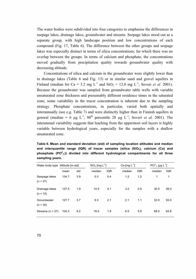
70

The water bodies were subdivided into four categories to emphasise the differences in

seepage lakes, drainage lakes, groundwater and streams. Seepage lakes stood out as a

separate group, with high landscape position and low concentrations of each

compound (Fig. 17, Table 6). The difference between the other groups and seepage

lakes was especially distinct in terms of silica concentrations, for which there was no

overlap between the groups. In terms of calcium and phosphate, the concentrations

moved gradually from precipitation quality towards groundwater quality with

decreasing altitude.

Concentrations of silica and calcium in the groundwater were slightly lower than

in drainage lakes (Table 6 and Fig. 13) or in similar sand and gravel aquifers in

Finland (median for Ca = 3.2 mg L-1 and SiO2 = 12.0 mg L-1; Soveri et al. 2001).

Because the groundwater was sampled from groundwater table wells with variable

unsaturated zone thickness and presumably different residence times in the saturated

zone, some variability in the tracer concentration is inherent due to the sampling

strategy. Phosphate concentrations, in particular, varied both spatially and

interannually (see e.g. Table 7) and were distinctly higher than in Finnish aquifers in

general (median = 6 µg L-1, 90th percentile 28 µg L-1; Soveri et al. 2001). The

interannual variability suggests that leaching from the uppermost soil layers is highly

variable between hydrological years, especially for the samples with a shallow

unsaturated zone.

Table 6. Mean and standard deviation (std) of sampling location altitudes and median

and interquantile range (IQR) of tracer samples (silica (SiO2), calcium (Ca) and

phosphate (PO43-)) divided into different hydrological compartments for all three

sampling years.

Water body type Altitude [m asl] SiO2 [mg L-1] Ca [mg L-1] PO43- [µg L-1]

mean std median IQR median IQR median IQR

Seepage lakes

(n = 27)

134.7 3.9 0.3 0.4 1.2 1.2 1 1

Drainage lakes

(n = 12)

127.5 1.9 14.5 4.1 3.2 0.9 30.5 28.0

Groundwater

(n = 30)

127.7 3.7 9.3 2.1 2.1 1.1 32.0 93.0

Streams (n = 27) 104.3 9.2 16.0 1.8 6.5 5.9 68.5 64.8

71

Streams were a distinctly separate group because of both their low landscape position

and high tracer average concentration and variability (Table 6). All the sampled

streams originated in the groundwater discharge area (Fig. 3) covered by peat soils.

During late winter, when the sampling was performed, streams receive very little

water from precipitation or surface runoff and most of their discharge can be assumed

to consist of base flow provided by the aquifer. Therefore it is reasonable to expect

that groundwater entering the streams as base flow has travelled along longer

subsurface flow paths than the water sampled from lakes and piezometers in the

recharge area. As a result, groundwater seepage to the streams is likely to be richer in

weathering compounds, which is in turn seen as elevated tracer concentrations in the

stream samples.

Phosphate concentration at a given sampling location showed a statistically

significant (p<0.001) monotonic Kendall’s correlation with both silica and calcium

concentrations (Fig. 18). The phosphate increased in a log-linear fashion with

increasing silica concentration, whereas the trend in correlation between phosphate

and calcium was less obvious but still monotonically increasing. Even though

phosphate concentration did not correlate strongly with landscape position in the

aquifer (Fig. 17), it nevertheless increased together with silica and calcium.

The finding is interesting, because even small differences in phosphate inputs can

change the ecological structure of sensitive surface water bodies. The subsurface is

traditionally considered a dilution system for phosphate, as in the study by Devito et al. (2000) which suggests that total phosphorus loading caused by forestry logging

and ending up in lakes is lower for lakes which receive groundwater via long

subsurface flow paths. Sorption processes responsible for dilution along long flow

paths can be expected if phosphorus concentration in the infiltrating water is elevated

significantly above the natural background concentration for some reason. However,

the results obtained in this thesis provide support for the claim made by Holman et al. (2010) that the subsurface can act as a source of phosphate in certain geological

settings, as also shown by Kidmose et al. (2013). This is best seen in the correlation

of phosphate with tracers indicating long residence time in the subsurface (Fig. 18).

72

Fig. 18. Crossplots of phosphate concentrations with silica (tau = 0.60, p<0.001) and

calcium (tau = 0.50, p<0.001). Reprinted with permission from Elsevier (Paper I).

Environmental tracers at lake (L3) and peatland catchment (S13) sites

Data on environmental tracer concentrations in the vicinity of L3 showed generally

higher concentrations of tracers at all groundwater sampling locations compared with

the lake (Table 7). Silica appeared to provide the strongest and most consistent signal

separating lake water from groundwater. It should be noted that cation concentrations

in inland piezometers may overestimate the concentrations in water actually

discharging to the lake (Brock et al. 1982, Krabbenhoft & Webster 1995).

Because the tracer concentrations in the lake do not resemble the concentrations

in the surrounding aquifer, the solute-rich groundwater input to lake water balance

seems to be of minor importance in comparison with solute-poor inputs from

precipitation. This conclusion is to some extent supported by the seepage meter

73

measurements, where the only consistent location of groundwater inflow was

observed in the south-east part of the lake. However, the tracer concentrations in L3

(Table 7) were slightly higher than in other seepage lakes in the area (Table 6), which

suggests there is more groundwater influence in L3 than in the average seepage lake.

Table 7. Concentrations of environmental tracers (silica (SiO2), calcium (Ca) and

phosphate (PO43-)) in Lake Ahveroinen (L3) and adjacent piezometers, 2010–2012.

Sampling

location

SiO2 [mg L-1] Ca [mg L-1] PO43- [µg L-1]

2010 2011 2012 2010 2011 2012 2010 2011 2012

L3 2.1 1.1 1.0 1.7 1.5 1.3 5 2 4

G6 9.4 10 11 1.8 3.4 3 6 550 350

G21 6.5 6.9 4 1.5 1.4 1.4 9 25 7

G20 7.9 8.7 8.5 1.4 2.3 2.1 99 130 20

G17 9.4 9.3 2.4 2.2 66 32

Environmental tracers showed a clear groundwater signal in surface water drainage

ditches in the groundwater discharge area (Fig. 19). The silica concentrations in

particular suggested that majority of the water in the drainage network originates from

the underlying sand aquifer with distinctly higher silica concentrations (7–16 mg L-1)

than in peat groundwater (1.2 mg L-1) or rainfall (<0.1 mg L-1). The tracer results also

showed the evolution of groundwater composition along the groundwater flow path

(Kenoyer & Bowser 1992). For all tracers used, the highest subsurface concentrations

were found in the confined sand aquifer most down-gradient in the catchment (G12a).

The lowest tracer concentrations in the sand aquifer were in G11, which most likely

has rapid input from rainwater because of the thin unsaturated layer (Fig. 19).

74

Fig. 19. pH and environmental tracers (SiO2, Ca2+ and EC) sampled from boreholes,

streams and precipitation in June 2010, plotted as the function of horizontal distance

from the first sample. Black columns are samples from the sand aquifer, white

columns represent the stream concentration at different locations and the grey

column is the groundwater in peat soil. Reprinted with permission from Elsevier

(Paper II).

75

5.1.3 Airborne thermal infrared imaging (IV)

The areal thermal imaging provided a spatially extensive snapshot of the GW-lake

exchange processes at the study site. Groundwater discharge to lakes in the Rokua

area was evident in the TIR data, since locations where water surface temperature was

notably cooler (10–15 °C) than the background temperature (~20 °C) were abundant

(Fig. 20). The data showed both diffuse groundwater inflow along long sections of the

shoreline and focused inflow coming from a more constrained area. Groundwater

inflow was observed in lakes throughout the aquifer recharge area and drainage lakes

with a stream outlet stood out, with a high number of groundwater inflow

observations.

Fig. 20. Spatial distribution of diffuse and concentrated groundwater discharge

locations in lakes in the Rokua aquifer recharge area.

76

5.1.4 Conceptual model for GW-SW interactions

Based on the results from field studies, the conceptual model of the aquifer hydrology

(Fig. 21) was verified for some parts (occurrence of GW-SW interaction) and refined

for other parts (spatial variability of GW-SW exchange and understanding of

groundwater flow systems). The field-based methods showed that:

– Groundwater-surface water interaction is unambiguously present between the

esker aquifer and related surface water bodies (Figs. 13 and 16)

– The interaction is highly variable in space in both lakes (Figs. 11 and 20) and

drainage channels (Fig. 16).

Use of environmental tracers:

– Further verified the small-scale GW-SW exchange processes (Table 7 and

Fig. 19)

– Facilitated generalisation of the small-scale exchange processes identified to

aquifer scale (Fig. 17)

– Showed that silica is a good tracer for groundwater influence in surface water

bodies for the given geology.

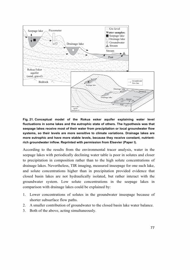
77

Fig. 21. Conceptual model of the Rokua esker aquifer explaining water level

fluctuations in some lakes and the eutrophic state of others. The hypothesis was that

seepage lakes receive most of their water from precipitation or local groundwater flow

systems, so their levels are more sensitive to climate variations. Drainage lakes are

more eutrophic and have more stable levels, because they receive constant, nutrient-

rich groundwater inflow. Reprinted with permission from Elsevier (Paper I).

According to the results from the environmental tracer analysis, water in the

seepage lakes with periodically declining water table is poor in solutes and closer

to precipitation in composition rather than to the high solute concentrations of

drainage lakes. Nevertheless, TIR imaging, measured inseepage for one such lake,

and solute concentrations higher than in precipitation provided evidence that

closed basin lakes are not hydraulically isolated, but rather interact with the

groundwater system. Low solute concentrations in the seepage lakes in

comparison with drainage lakes could be explained by:

1. Lower concentrations of solutes in the groundwater inseepage because of

shorter subsurface flow paths.

2. A smaller contribution of groundwater to the closed basin lake water balance.

3. Both of the above, acting simultaneously.

78

Environmental tracers were present in similar concentrations in eutrophic

drainage lakes and in groundwater, implying nutrient and cation input to certain lakes

from groundwater discharge. Surface or near surface runoff is often considered an

important transport route for nutrients to surface water bodies, but at the study site

highly permeable soils and a lichen layer covering the soils make the surface runoff in

the area negligible. Among possible anthropogenic sources, agriculture in the aquifer

recharge area is non-existent. Forestry activities, which have been shown to be a

potential source of e.g. phosphate to groundwater (Devito et al. 2000), are practised in

the area. However, fertilisation in the forestry has been minimal and the nutrient

leaching from the forestry is estimated to be at the level of natural background

loading (Väisänen et al. 2007). Because land use practices and habitation in the

catchment areas of seepage and drainage lakes are similar and nutrient inputs to the

system from precipitation almost non-existent, subsurface origin by leaching,

dissolution, weathering or desorption remains the most credible source providing

nutrients and cations to the lakes.

A considerable body of research reports similar inputs of dissolution and

weathering products to lakes via long, regional groundwater flow paths (Brock et al. 1982, Kenoyer & Anderson 1989, Kenoyer & Bowser 1992, Webster et al. 1996). In

the Rokua aquifer area, stream outlets are a vital component in enabling and

sustaining steady, nutrient-rich groundwater inflow to the drainage lakes. This holds

true especially for the first lakes in the chain of lakes, which have no inlets but

discharge water constantly via outlets. These outlets convey the nutrient-rich water

seeping from groundwater through the chain of lakes, affecting the water quality of

the whole lake chain. Stets at al. (2010) have reported similar settings where a

regional groundwater flow system provides inflow to headwater lakes connected with

streams.

5.2 Spatially and temporally distributed groundwater recharge (III)

Spatial and temporal variations in groundwater recharge were estimated with a

modelling approach developed to utilise forestry inventory data. The Richards

equation-based 1-D simulations were spatially distributed using Monte Carlo runs for

an unsaturated soil column. Within the Monte Carlo process, residence time in the

unsaturated zone and relevant physical characteristics of the system were accounted

for, while uncertainty in selected model parameters was propagated to the final

recharge time series. The simulations provided a sound estimate for historical time

series of groundwater recharge in the Rokua esker aquifer.

79

5.2.1 Model validation

The model showed reasonable performance and consistency when compared

against independent recharge estimates obtained with both WTF and baseflow

methods (Fig. 22 and Table 8, respectively). The WTF method agreed well with

the simulated values, with overlapping estimates between the methods for all but

two boreholes. Moreover, the median value of simulations was close to that

obtained with the WTF method, but with some bias towards higher estimates

from the simulations.

The discrepancy can be due to different assumptions behind the methods and

uncertainty in local parameterisation, in the WTF method for the specific yield and in

the simulations mainly for the hydraulic conductivity, which dictates the timing of

recharge. However, there were overlapping estimates for almost every recharge event,

which shows consistency between the methods. The stream baseflow was lower than

the long-term average recharge, which was expected because of the site

hydrogeology. All of the outflow from the aquifer was probably not captured by the

baseflow measurements, as some of the water discharges to larger streams and lakes

outside the stream catchments (as shown in Section 5.3). When simulated recharge

was extracted specifically for the baseflow measurement dates, the lower values for

simulated recharge were also anticipated because of seasonal variability in recharge

but a stabilising effect of the groundwater storage for stream baseflow. In conclusion,

the order of magnitude of the regional baseflow estimates and the simulation results

was similar. Despite the very different assumptions on which the modelling and field

methods were based, all provided similar estimates of groundwater recharge at the

study site.

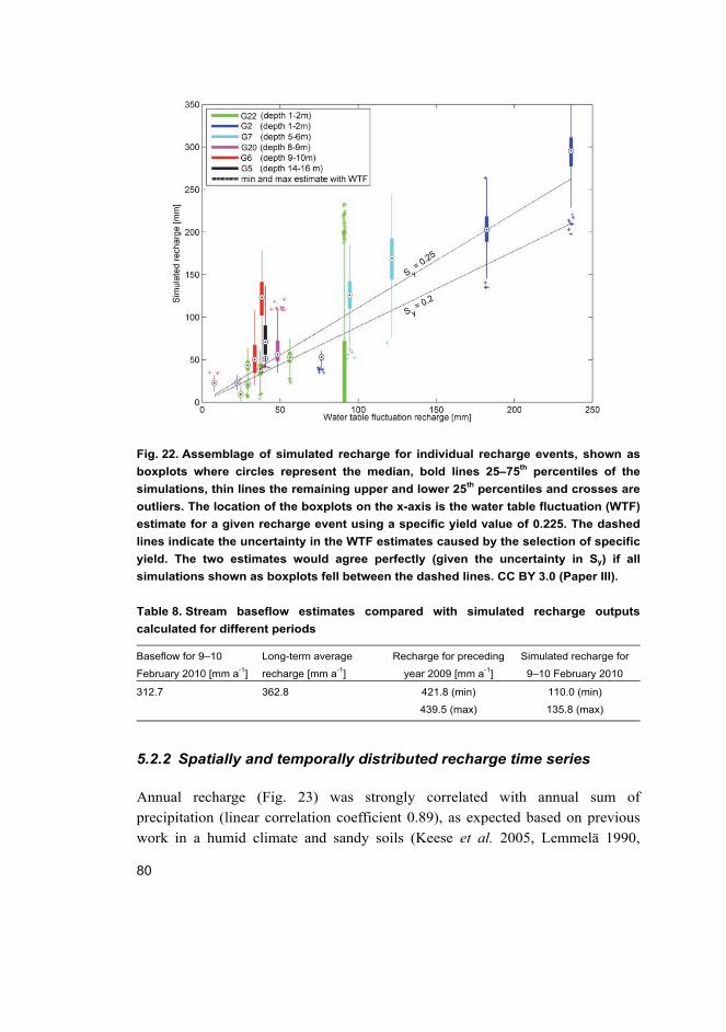
80

Fig. 22. Assemblage of simulated recharge for individual recharge events, shown as

boxplots where circles represent the median, bold lines 25–75th percentiles of the

simulations, thin lines the remaining upper and lower 25th percentiles and crosses are

outliers. The location of the boxplots on the x-axis is the water table fluctuation (WTF)

estimate for a given recharge event using a specific yield value of 0.225. The dashed

lines indicate the uncertainty in the WTF estimates caused by the selection of specific

yield. The two estimates would agree perfectly (given the uncertainty in Sy) if all

simulations shown as boxplots fell between the dashed lines. CC BY 3.0 (Paper III).

Table 8. Stream baseflow estimates compared with simulated recharge outputs

calculated for different periods

Baseflow for 9–10

February 2010 [mm a-1]

Long-term average

recharge [mm a-1]

Recharge for preceding

year 2009 [mm a-1]

Simulated recharge for

9–10 February 2010

312.7 362.8 421.8 (min) 110.0 (min)

439.5 (max) 135.8 (max)

5.2.2 Spatially and temporally distributed recharge time series

Annual recharge (Fig. 23) was strongly correlated with annual sum of

precipitation (linear correlation coefficient 0.89), as expected based on previous

work in a humid climate and sandy soils (Keese et al. 2005, Lemmelä 1990,

81

Okkonen & Kløve 2011). According to the simulations, the average groundwater

recharge was 362.8 mm year-1, and the effective rainfall, i.e. the percentage of

rainfall resulting in groundwater recharge annually, was on average 59.3%. This

is in agreement with previous studies on unconfined esker aquifers at northerly

latitudes, in which the proportion of annual precipitation percolating to recharge

is reported to be 50–70% (71% by Zaitsoff (1984), 54% by Lemmelä and Tattari

(1986) and 56% by Lemmelä (1990)).

Fig. 23. Annual recharge time series from simulations, where the black area covers the

minimum and maximum values for different recharge samples. The annual recharge

pattern closely followed trends in infiltration. Effects of different land use

management practices over time on annual recharge rates are shown as high and low

leaf area index (LAI) scenarios. CC BY 3.0 (Paper III).

The method used here to estimate LAI from forestry inventories introduces a new

approach for incorporating large spatial coverage of detailed conifer canopy data into

groundwater recharge estimations. The spatial distribution of groundwater recharge

was indeed mostly due to variations in LAI originating from forestry data, distance to

water table and distribution of lakes (Fig. 24). Higher evaporation rates from lakes led

82

to lower recharge in lakes (see red spots in Fig. 24). Similarly, high LAI led to high

ET and resulted in low recharge. Other areas of low recharge, although not as obvious

at the larger spatial scales shown in Fig. 24, were cells with a shallow water table. The

effect of high ET at locations with a shallow water table can best be seen in south-east

parts of the aquifer.

Fig. 24. Spatial distribution of mean annual recharge, which was influenced mainly by

the Scots pine canopy (leaf area index, LAI), the presence of lakes and, to some

extent, areas with a shallow water table. CC BY 3.0 (Paper III)

Estimated evaporation from the land surface (mean 237.6 mm) was somewhat

lower than previous regional estimates of total ET (300 mm; Mustonen 1986).

Kelliher et al. (1998) found that ET from boreal conifer forests is around 2 mm d-

1 during the growing season, which is again slightly higher than our average value

of 1.6 mm d-1 for the period 1 May–31 Oct. The differences may have been

caused by the permeable sandy soil type at the study site. Conifer forests in the

boreal zone are usually dominated by less permeable glacial till soils, allowing

83

more time for evaporation before percolating below root zone. More details about

the allocation of evaporation to different components are given in Paper III.

5.2.3 Impact of LAI on groundwater recharge

Plant cover, represented as LAI, proved to be the most important model parameter

determining the total recharge amount (Fig. 25). This has been reported in earlier

simulation studies estimating groundwater recharge (Dripps 2012, Keese et al. 2005,

Sophocleous 2000), but here the vegetation was represented with more spatially

detailed patterns and a field data-based approach for LAI. However, some earlier field

studies have claimed that the influence of LAI on total ET rates from boreal conifer

canopies is minor (Kelliher et al. 1993, Ohta et al. 2001, Vesala et al. 2005). There

appears to be a disagreement in the literature, with field studies suggesting that total

ET is not much influenced by canopy LAI, whereas modelling studies such as the

present thesis demonstrate a clear increase in ET with increasing LAI. Therefore more

work is needed in matching the model estimates and field data for conifer ET. While

soil (and snow) evaporation partly compensated for the lower transpiration for LAI

values up to around 1.0, the total annual ET values progressively increased as a

function of LAI (Fig. 25). Interestingly, the simulations suggested that ET remains

constant in the LAI range 0–1, potentially due to the sparse canopy changing the

aerodynamic resistance and partitioning of radiation limiting soil evaporation, while

still not contributing much to transpiration in total ET. This suggests that the

maximum groundwater recharge for boreal Scots pine remains rather constant up to a

threshold LAI value of around 1. This knowledge can be used when co-managing

forest and groundwater resources in order to optimise both.

84

Fig. 25. Example of scatter plots with the mean annual evapotranspiration (ET)

components are plotted as a function of the variable leaf area index (LAI), showing

clear dependence of all ET components on LAI. CC BY 3.0 (Paper III).

LAI values reported for conifer forests in Nordic conditions similar to the study site

are in the range 1–3, depending on canopy density and other attributes (Koivusalo et al. 2008, Rautiainen et al. 2012, Vincke & Thiry 2008, Wang et al. 2004). The LAI

values obtained for the study site (mean 1.25) were at the lower end of this range.

Furthermore, the data showed a bimodal distribution, with many model cells with low

LAI (<0.4) lowering the mean LAI (Fig. 12). The low LAI values were not

considered to be an error in data or calculations, but were in fact expected because of

active logging and clear-cutting in the study area. Although the equations to estimate

LAI are empirical in nature and based on simplified assumptions, the method can

outline spatial differences in canopy structure. However, the LAI estimation method

could be further validated with field measurements or LiDAR techniques (Chasmer et al. 2012, Riaño et al. 2004).

The method allowed different land use scenarios in forestry management to be

tested. The simulations showed that variable intensity of forestry, from low canopy

coverage (LAI = 0–0.2) to dense coverage (LAI = 3.2–3.5), resulted in an average

difference of 101.7 mm in annual recharge (Fig. 24). It can be argued that the

85

scenarios are unrealistic, because high LAI values, covering the whole study site, may

not be achieved even with a complete absence of forestry operations. Nevertheless,

the results demonstrate a substantial impact of forestry operations on esker aquifer

groundwater resources. Previous work on the subject focused on changes in

groundwater quality (Kubin 1998, Mannerkoski et al. 2005, Rusanen et al. 2004),

whereas our simulations also have quantitative implications. However, more work

should be done on comparing field and model estimates for conifer stand ET fluxes.

5.3 Surface-subsurface flow modelling of GW-lake interactions (IV)

A fully integrated surface-subsurface groundwater model was established to simulate

the transient hydrological processes in the esker aquifer, with particular emphasis on

the fluxes at the GW-SW interface. The model successfully reproduced the

hydrological processes of a complex esker aquifer with seepage and drainage lakes

and interconnected streams in both steady state and transient mode. The simulation

results provided information on GW-lake interactions which were validated with field

measurements.

Water balance over the 13-year simulation period was distributed between: (1)

Water input as rainfall and snowmelt (632 mm year-1), (2) evapotranspiration (297

mm year-1), (3) surface water outflow from the critical depth boundary condition (251

mm year-1), (4) subsurface outflow from the specified head boundary condition (79

mm year-1), and (5) net accumulation of water in the model domain (5 mm year-1).

The values for annual precipitation and ET are typical for the study site area

(Mustonen 1986). The model provided novel estimates of the amount of aquifer

groundwater discharge from a complex shallow aquifer to regional surface water

bodies. The River Oulujoki (Fig. 3) receives the majority (69.6 mm year-1) of the

subsurface discharge, which was expected because of steepest gradients and deepest

overburden layers at the boundary. Water accumulation in the model domain reflected

the increase in storage due to elevated groundwater levels during the simulation

period.

The model successfully reproduced the main dynamics in hydraulic head and

stream flow in both transient and steady state mode. A detailed comparison of

simulations and observations is given in Paper IV. Of the alternatives given in

Table 3, hydraulic conductivity of 2 x 10-5 m s-1 and an anisotropy ratio of 1:2 gave

the best agreement between GW and lake head and stream outflow. Absolute mean

error for simulated and observed GW and lake head was 2.38 m and 2.94 m,

respectively. Errors of similar magnitude have been reported in earlier catchment-

86

scale surface-subsurface modelling studies (Goderniaux et al. 2009, Jones et al. 2008,

Sudicky et al. 2008). The simulated head values were positively biased (simulated

higher than measured) above 130 m asl. For all other calibration alternatives (Table

3), the GW and lake levels were underestimated, whereas the selected combination

led to a slight general overestimation. Thus the most representative value for

hydraulic conductivity and anisotropy was found in the lower end of the calibration

range. A better fit could be obtained by adjusting the K value in the range 6.5 x 10-5 –

2 x 10-5 m s-1, while keeping the anisotropy at 1:2. The simplifying assumption of

homogeneous K throughout the aquifer inevitably introduced error into the

simulations. Local-scale heterogeneities in the subsurface are undoubtedly present

and could be captured by automated model calibration schemes, as done in another

modelling study of the area (Rossi et al. 2014).

This thesis demonstrates the ability of the fully integrated hydrological

simulation code HydroGeoSphere to represent the study site hydrological system at

aquifer scale, while maintaining detailed simulations of GW-SW interactions in the

model set-up. Previous fully integrated modelling studies have focused mainly on

simulating domains delineated by surface water catchments (Goderniaux et al. 2009,

Jones et al. 2008, Li et al. 2008). When modelling work has focused on lake systems,

the models rarely cover the full extent of an aquifer (Kidmose et al. 2013, Smerdon et al. 2007, Virdi et al. 2013). The surface water bodies here were defined in the model

only as topographical features derived from DEM and bathymetric maps, and the

model routed water into lakes and streams in accordance with field measurements.

The good level of general model performance provides more confidence about using

fully integrated surface-subsurface models as a tool to simulate esker aquifers with

interconnected lakes, streams and wetlands.

5.3.1 GW-lake interaction: discharge locations and fluxes

Spatially distributed groundwater inflow to lakes

To the best of my knowledge, this is the first study to compare the results of airborne

thermal imaging with those of numerical simulations in a system of lakes. The general

pattern of groundwater inflow locations to lakes, interpreted from areal thermal

imaging, was captured by the simulations (Fig. 26). In most areas where TIR data

showed groundwater discharge, there were also model nodes showing positive

exchange flux between subsurface and surface domains. For example, in lake L9,

87

which continously drains the aquifer, both observations and simulations showed

groundwater discharge almost throughout the lake perimeter. The same was true for

L8, although not apparent in detail because of smaller lake size. Only a few locations

of groundwater inflow were missed by the simulations, for example in the north-east

part of lakes L3, L4 and L11. The inability of thermal imaging to capture all

groundwater discharge locations is best seen in lake L12, for which both simulations

and isotope methods showed a clear signal of groundwater inflow (Fig. 27), but the

TIR data did not reveal inflow locations to the lake (Fig. 26).

Fig. 26. Locations of observed groundwater inflow from areal thermal imaging, which

compared well with model cells where groundwater inflow was simulated.

The differences between simulated and observed groundwater inflow locations

are mainly attributable to difficulties in observing groundwater inflow in thermal

imaging data (see Section 4.1.4), model mesh resolution, simplified geological

model and model overestimation of groundwater head. Model mesh resolution

was refined for the lakes with monitoring, but the topographical relief

surrounding the lakes was still not fully captured. Therefore some local

groundwater mounds around lakes may not be adequately represented in the

88

model, and some observed localised groundwater inflow may not be reproduced.

In addition, some of the lake beds consisted of only a couple of cells (e.g. L4, L5,

L6, L11) and the model resolution was too coarse to simulate the groundwater

inflow focused near the lake shoreline in those cases. Finally, local subsurface

heterogeneities and the distribution of lake bed sediments can have a great effect

on GW-SW exchange locations (Kidmose et al. 2013, Smerdon et al. 2005).

Because soil and lake bed were represented with uniform hydraulic

parameterisation, GW-SW exchange hotspots due to local heterogeneities were

overlooked by the simulations.

Comparison of simulated and calculated groundwater influxes to lakes

In addition to similarity in spatial distribution, the magnitude of simulated

groundwater inflow flux showed agreement with the inflow determined using

stable isotope methods (Fig. 27). The magnitude of inflow ranged from tens to

thousands of m3 s-1, the highest inflow being in L9 constantly draining via outlet

S3. The simulations gave a good estimate of the order of magnitude in

groundwater inflow, although some mismatches occurred in the absolute values. A

better match between simulated and observed hydraulic head would probably

bring the values even closer together. This result is promising, because total

groundwater inflow is a difficult variable to estimate in a lake water balance. In

the absence of surface runoff and stream inlets in particular, groundwater inflow

can be the main source of nutrients in the lake water balance (Holman et al. 2010,

Kidmose et al. 2013, Winter et al. 1998). Therefore a valid model-based estimate

of the magnitude and spatial distribution of the groundwater influx, along with

information on groundwater quality, can provide crucial information on

ecologically relevant fluxes needed in current water resources management.

89

Fig. 27. Calculated groundwater influx to various lakes in August 2013 using the stable

isotope method (Isokangas et al. 2014) and the corresponding simulated groundwater

influx values.

The overall overestimation of groundwater head above 130 m asl can be seen as

biased results in several GW-SW exchange outputs. Higher than observed head

can be expected to provide excess groundwater discharge to lakes, especially

drainage lakes. Because the outlet elevation is defined from the DEM draining the

lake above the defined altitude, the increased hydraulic gradient due to head

overestimation leads to increased groundwater influx. In the spatial distribution of

groundwater discharge, this conclusion is supported by the most northerly lakes

connected by a stream starting at L8. There, simulations showed extensive

groundwater discharge to south-east parts of the lakes, whereas only little inflow

was seen in areal thermal imaging (Fig. 26). Similar overestimation can be

inferred for drainage lakes L8, L9 and L10 in terms of total influx (Fig. 27),

where the simulations showed consistent overestimation. In reality, lake L10 did

not have an outlet during the observation period (see Fig. 26), but closer

examination of the simulation outputs showed an ephemeral surface flow

connection emerging from lake L10 to L8. Thus the fully integrated modelling

approach created a lake outlet in a physically based manner, where the

90

groundwater level reached the ground surface. The emerging outlet allowed

seasonal draining of the lake, and thereby excess groundwater discharge. Finally,

excess groundwater influx could be seen to some extent in stream flow, as flow

rate overestimation for some of the streams which act as lake outlets (S3, S18 and

S19).

5.3.2 Simulated transient variability in the GW-lake interaction

The fully integrated modelling approach enabled extraction of influx time series

between lakes and groundwater. The time series of groundwater inflow showed both

annual (seasonal) and interannual (long term) variability, which appeared to be

different among lakes in the area (Fig. 28). Drainage lakes (L8, L9, and L10)

exhibited different dynamics for groundwater inflow than seepage lakes. The level of

seepage lakes followed the groundwater level, showing a similar decreasing trend

until 2004 with a following rise until the end of simulations (see Fig. 4 in Paper IV).

These changes can be attributed to natural climate variability, with drier conditions at

the beginning of the simulation period. The water levels in drainage lakes, on the

other hand, were kept relatively constant by the base of the outlet, as discussed earlier.

This made the hydraulic gradient between lakes and groundwater decrease and

increase according to the position of the groundwater table, creating interannual

variability in groundwater inflow. For the seepage lakes, the lake water levels rose at

approximately same rate as the groundwater level, therefore keeping the hydraulic

gradient and influx more stable in the long term. Groundwater inflow trends are much

more variable in closed basin lakes, with an increasing trend in some (L3, L11, L12)

and a declining trend in others (L5, L6). Hunt et al. (2013) reported similar

differences in transient lake inflow response between drainage and seepage lakes in

their lake system modelling study.

91

Fig. 28. Transient groundwater inflow to lakes, showing both seasonal and interannual

variability. The time series are plotted as standardised values to facilitate comparison

between different lakes (L1–L12).

Several field methods enable the estimation of groundwater influx time series on a

small scale (Kalbus et al. 2006, Rosenberry & LaBaugh 2008), but studying and

comparing transient influxes for a lake system would be highly laborious, if possible

at all, with current techniques. Given that the model reproduced the spatial locations

and flow volumes with acceptable accuracy, the transient variability in groundwater

inflow can be studied in a meaningful way. However, it should be noted that the flux

time series plotted in Fig. 28 were extracted from cells which exhibited groundwater

inflow on 1 Aug 2013, to facilitate prior comparison with thermal imaging and stable

isotope data. Some of the selected cells may seasonally shift in flow direction from

inseepage to outseepage, whereas other cells showing outseepage on 1 Aug 2013 may

seasonally become inseepage cells at other times. Therefore the time series most

likely did not capture the full amplitude of the annual variability. However, closer

examination of the shifting cells in model output showed that flux in those was

generally some orders of magnitude lower than in cells of permanent high inseepage

selected for output (see red dots in Fig. 26). Thus Fig. 28 gives a good indication of

the overall dynamics of the groundwater inflow into lakes at the study site.

92

Groundwater influx appeared to follow the groundwater table hydrograph

typically found at latitudes with seasonal snow cover, such as the study site, except

for the distinct and sudden decline in inflow at the onset of snowmelt (Fig. 29). This

sudden decline appears to be physically unrealistic, but can be explained by how the

model surface boundary conditions were executed. Water input from the snowmelt

was simulated in Coup Model (Section 5.2) and acted as input to the current HGS

model application. The input was defined as specified flux to the entire model top

domain, including lakes. Therefore the free water surface at inundated lake nodes

received the snowmelt water immediately, with perhaps some additional contribution

from overland flow, whereas the response of the groundwater level was delayed due

to the unsaturated layer. In reality, lake snow and ice cover is readily included in total

hydraulic head for a given point, because the snow and ice are primarily ‘floating’ on

the lake. The sudden increase in simulated lake head presumably levelled out the

difference between the upgradient groundwater table and lake momentarily, ‘pushing

back’ the groundwater inflow. After the sudden shock, the head stabilised and

snowmelt reached the groundwater level, resulting in the expected increase in

groundwater influx.

93

Fig. 29. Annual cycle for lake groundwater inflow, resembling a typical groundwater

(GW) hydrograph and starting with declining inflow rates for Jan-April (1). At the onset

of snowmelt, typically in early May (2), GW inflow decreased rapidly and quickly

turned to elevated inflow (3); the amplitude of these shifts varied for different lakes

(Fig. 8). Inflow started to decrease towards summer, with flow minima typically found

in July (4). Inflow started to increase towards autumn (5), because of lower

evapotranspiration and higher precipitation leading to rising GW levels.

When simulated GW-SW exchange flux was compared with the seepage meter

measurements in L3 (Section 5.1.1), the latter showed a very similar distribution of

groundwater inflow and outflow locations as simulated in the present thesis. The

measured groundwater inflows were also of the same order of magnitude as the

simulations. For example, the largest measured average inflow at the south-east

corner of the lake during summer 2010 was 5.7 x 10-7 m s-1, while the simulations for

the same period gave an average positive exchange flux of 3.3 x 10-7 m s-1. As a

peculiarity, a preliminary round of seepage measurements in 2009 showed

groundwater inflow from the north-west part of the lake. The later seepage meter

measurements in slightly different locations during 2010 did not confirm the 2009

results, and the simulations did not result in inflow for the northern parts of the lake.

Nonetheless, the areal thermal imaging interestingly showed a spot of groundwater

94

inflow at approximately the same location as measured in 2009. This demonstrates

that exchange fluxes between GW and SW are highly variable in space and time and

very difficult to characterise unambiguously, even by using several independent

methods.

95

6 Conclusions and future recommendations

This thesis combined multiple field investigations and state-of-the-art numerical

groundwater modelling methods to study hydrological processes in a complex

esker aquifer. The research focused on the largely unknown interaction between

the Rokua esker aquifer and lakes and streams located in the area. In addition to

providing information on GW-SW exchange, the thesis enhanced the

understanding of esker aquifer hydrology in terms of water quality and water

budgets for both whole aquifer and single water body scale.

Paper I verified GW-lake interactions in the area with seepage meters and used

environmental tracers to show the variable presence of groundwater in other lakes and

streams in the area. Paper II studied GW-peatland interaction and demonstrated the

role of peatland drainage in amplifying groundwater outflow from the aquifer. Paper

III used numerical simulations to establish the influence of forestry land use and

aquifer geometry on groundwater recharge. Paper IV merged the established process

understanding and collected field data into a fully-integrated surface-subsurface flow

model, which was used to simulate spatial variability, total inflow fluxes and transient

changes in GW-lake interaction.

Both field and numerical studies highlighted that the GW-SW interactions in

Rokua esker aquifer were highly variable in space for both lakes and streams. The

groundwater discharged into lakes (in the groundwater recharge area) and peatland

drainage ditches (in the groundwater discharge area) in very complex patterns.

Discharge occurred both as focused flow in specific, spring-like locations and diffuse

seepage covering a larger areal extent in both lakes and streams. Because of process

complexity, investigations to understand detailed patterns of groundwater exfiltration

into surface water bodies will remain a laborious task in esker aquifers.

At the Rokua esker, the GW-SW exchange process appeared to be more stable in

time than in space. Therefore tools that can integrate the observed sporadic spatial

variability into total fluxes over a larger spatial extent have great potential in studying

the influence of groundwater on surface water bodies. The most prominent tool used

in this thesis was fully integrated surface-subsurface flow modelling. The method

provided estimates of the strength of groundwater inflow to surface water bodies

which were consistent with field observations. However, all the field and modeling

methods used in this thesis were helpful in establishing the conceptual process

understanding needed in the integrated flow modelling. Therefore use of multiple

methods for GW-SW interaction studies in esker aquifers is strongly recommended.

96

This thesis provides new information on the site-specific problems in the Rokua

esker aquifer. Seepage lakes (lakes without outlets) have suffered periodically

declining water levels, whereas the drainage lakes (lakes with outlets) have shown

eutrophic water quality. Both these phenomena negatively affect the recreational use

of the lakes, but they are also considered a threat to lake ecosystems. Water level

variability in the transient surface-subsurface flow simulations agreed relatively well

with the observed lake level changes. Therefore at least the most recent lake level

decline (during the early 2000s) can be explained by climate variability, because no

land use changes were included in the simulations. Rossi (2014) reached a similar

conclusion, that the majority of the lake level variability can be explained by climate

factors. However, peatland ditches may have a long-term draining effect on the

aquifer, but this could not be verified in this thesis.

The role of groundwater as a nutrient source for Rokua’s lakes was clarified in

this thesis. The eutrophic status of drainage lakes is most likely related to nutrient-rich

groundwater discharging to the lakes. The drainage lakes and groundwater are

similarly enriched not only in nutrients (phosphate), but also in soil weathering

products (silica, major cations), indicating groundwater input into the lakes. Notable

groundwater inflow to the drainage lakes was also shown by the numerical modelling.

The subsurface loading of nutrients carried by groundwater is nearly impossible to

prevent, which has implications for surface water management practices. The results

presented in this thesis suggest that groundwater inflow results in naturally eutrophic

lakes in Rokua. This emphasises the need for integrated groundwater-surface water

management, because neglecting the groundwater as a source of phosphorus influx to

lakes would lead to misinformed management decisions. This thesis provides new

knowledge on the potential role of groundwater on lake water quality when the lake is

a part of complex esker aquifer system. However, the role of groundwater in surface

water bodies will be different in other esker aquifers, both qualitatively and

quantitatively, and therefore the results presented here cannot be generalised directly

to other esker environments. Nevertheless, the methods applied in this work can be

used to study site-specific hydrology in esker aquifers and address local management

issues.

This thesis produced new information on how forestry land use can influence

hydrological processes in esker aquifers. Forestry was found to affect the aquifer

water storage in two opposing ways. Open drainage channels, excavated to drain the

peat soil, have the unintended potential to also drain the underlying confined aquifer

in groundwater discharge areas. In groundwater recharge areas, on the other hand, the

main forestry operation is forestry logging. The simulations in this thesis suggest that

97

thinning or removing the tree canopy can result in an increase of 100 mm (30%) in

groundwater recharge. Therefore land use actions can both decrease and increase

groundwater storage. This adds to the previous statement that esker aquifers should be

understood and managed as a single unit.

Proposals for future studies

Based on the results presented in this thesis, the following research topics would

further increase the understanding of esker aquifer hydrology:

– Changes in GW-SW interaction fluxes due to water abstraction should be

tested with integrated surface-subsurface modelling methods. Such work

would be beneficial in water resources management, where the impacts of

water abstraction on the GW-SW interface are poorly understood and

quantified.

– Rigorous automated model calibration and uncertainty estimation schemes

need to be implemented in surface-subsurface models to understand the

impact of model parameter uncertainty on the GW-SW exchange fluxes.

Groundwater model calibration efforts usually focus on matching

groundwater head and stream hydrographs, but novel methods, such as TIR

and stable water isotopes, would enable the actual exchange fluxes to be used

as a calibration objective.

– More attention should be paid to mechanisms of groundwater exfiltration to

peatlands, where the groundwater discharge via preferential flowpaths in

particular is poorly understood. Detailed field investigations in other aquifers

would be needed to quantify the relevance of the phenomena shown here for

esker aquifer management in general.

– More work should be done on comparing model and field-based ET estimates

for boreal conifer canopies. The coupling of the vegetation-atmosphere

boundary to the otherwise well-integrated surface-subsurface simulations

could also be further developed.

This thesis provides an example of successful combination of field techniques and a

fully integrated surface-subsurface model (HGS) application in a water resource

problem. These numerical modelling techniques can provide data-based estimates on

spatially and temporally variable fluxes of water, heat and nutrients, which determine

the environmental conditions for ecological communities. This information will be

increasingly called for in future water resources management, as the importance of

98

groundwater-dependent ecology is stressed in European Union and Finnish water

legislation. The work presented in this thesis will hopefully promote the use of novel

numerical simulation methods in studying esker aquifer hydrology. To fully exploit

the potential of the methods presented here, more interdisciplinary research involving

hydrology and ecology is needed for combined management of ecology and water

resources. Future research efforts in esker aquifer hydrology should focus on

establishing the role of groundwater in ecology related to esker aquifers.

99

References

Aartolahti T (1973) Morphology, vegetation and development of Rokuanvaara, an esker and dune complex in Finland. Fennia, 127. Helsinki, Societas geographica Fenniae.

Ajami H, McCabe MF, Evans JP & Stisen S (2014) Assessing the impact of model spin-up on surface water-groundwater interactions using an integrated hydrologic model. Water Resour Res 50(3): 2636–2656.

Allen R, Pereira L, Raes D & Smith M (1998) Crop evapotranspiration - Guidelines for computing crop water requirements. FAO irrigation and drainage paper No. 56. Rome, Food and Agriculture Organization of the United Nations.

Anderson MP & Cheng X (1993) Long-and short-term transience in a groundwater/lake system in Wisconsin, USA. J Hydrol 145(1–2): 1–18.

Anderson MP (2005) Heat as a ground water tracer. Groundwater 43(6): 951–968. Anibas C, Buis K, Verhoeven R, Meire P & Batelaan O (2011) A simple thermal mapping

method for seasonal spatial patterns of groundwater–surface water interaction. J Hydrol 397(1): 93–104.

Anttila EL & Heikkinen ML (2007) Surface water and groundwater levels, and changes in water levels at Rokua area (in Finnish). In: Heikkinen M & Väisänen T (eds) Lakes and ponds at Rokua area, North Ostrobothnia Regional Environment Centre reports 5 | 2007. Oulu, Finland, North Ostrobothnia Regional Environment Centre: 12–25.

Aquanty (2013) HydroGeoSphere User Manual. Release 1.0. Waterloo, Ontario, Canada, Aquanty Inc.

Assefa KA & Woodbury AD (2013) Transient, spatially varied groundwater recharge modelling. Water Resour Res 49: 1–14.

Ataie-Ashtiani B, Volker R & Lockington D (1999) Tidal effects on sea water intrusion in unconfined aquifers. J Hydrol 216(1): 17–31.

Banerjee I (1975) Nature of esker sedimentation. In: Jopling AV & McDonald BC (eds) Glaciofluvial and glaciolacustrine sedimentation. Tulsa, U.S.A., Soc. Econ. Paleontol. Mineral.: 132–155.

Barwell VK (1981) Determination of horizontal-to-vertical hydraulic conductivity ratios from seepage measurements on lake beds. Water Resour Res 17(3): 565–570.

Bertrand G, Siergieiev D, Ala-Aho P & Rossi PM (2013) Environmental tracers and indicators bringing together groundwater, surface water and groundwater-dependent ecosystems: importance of scale in choosing relevant tools. Environ Earth Sci 72: 813–827.

Blum OB (1973) Water relations. In: Ahmadjian V & Hale ME (eds) The lichens. USA, Academic Press Inc.: 381–397.

Bolduc A, Paradis SJ, Riverin M, Lefebvre R & Michaud Y (2005) A 3D esker geomodel for groundwater research: the case of the Saint-Mathieu–Berry esker, Abitibi, Quebec, Canada. Three-Dimensional Geologic Mapping for Groundwater Applications: workshop extended abstracts. Ottawa, Geological survey of Canada: 17–20.

100

Britschgi R, Antikainen M, Ekholm-Peltonen M, Hyvärinen V, Nylander E, Siiro P & Suomela T (2009) Mapping and classification of groundwater areas (in Finnish). Environment Guide | 2009. Sastamala, Finland, Finnish Environment Institute.

Brock TD, Lee DR, Janes D & Winek D (1982) Groundwater seepage as a nutrient source to a drainage lake; Lake Mendota, Wisconsin. Water Res 16(7): 1255–1263.

Brodie R, Sundaram B, Tottenham R, Hostetler S & Ransley T (2007) An overview of tools for assessing groundwater-surface water connectivity. Canberra, Bureau of Rural Sciences.

Brookfield A, Sudicky E, Park Y & Conant B (2009) Thermal transport modelling in a fully integrated surface/subsurface framework. Hydrol Process 23(15): 2150–2164.

Brown J, Bach L, Aldous A, Wyers A & DeGagné J (2010) Groundwater-dependent ecosystems in Oregon: an assessment of their distribution and associated threats. Front Ecol Environ : doi: 10.1890/090108.

Brunner P & Simmons CT (2012) HydroGeoSphere: a fully integrated, physically based hydrological model. Ground Water 50(2): 170–176.

Brunner P, Simmons CT, Cook PG & Therrien R (2010) Modeling Surface Water-Groundwater Interaction with MODFLOW: Some Considerations. Groundwater 48(2): 174–180.

Cable JE, Burnett WC & Chanton JP (1997) Magnitude and variations of groundwater seepage along a Florida marine shoreline. Biogeochemistry 38(2): 189–205.

Chasmer L, Pertrone R, Brown S, Hopkinson C, Mendoza C, Diiwu J, Quinton W & Devito K (2012) Sensitivity of modelled evapotranspiration to canopy characteristics within the Western Boreal Plain, Alberta. Remote Sensing and Hydrology 2010 held at Jackson Hole, Wyoming, USA. Oxfordshire, UK, IAHS Publ. 352: 337–340.

Cherkauer DA & McBride JM (1988) A remotely operated seepage meter for use in large lakes and rivers. Ground Water 26(2): 165–171.

Cherkauer DS & Nader DC (1989) Distribution of groundwater seepage to large surface-water bodies: The effect of hydraulic heterogeneities. J Hydrol (Amst ) 109(1): 151–165.

Cherkauer DS & Zager JP (1989) Groundwater interaction with a kettle-hole lake: Relation of observations to digital simulations. J Hydrol 109(1): 167–184.

Clark ID & Fritz P (1997) Environmental isotopes in hydrogeology. New York, USA, Lewis Publishers.

Conant B (2004) Delineating and quantifying ground water discharge zones using streambed temperatures. Groundwater 42(2): 243–257.

Darcy H (1856) Les Fontaines Publiques de la Ville de Dijon. Victor Dalmont, Paris. Devito KJ, Creed IF, Rothwell RL & Prepas EE (2000) Landscape controls on phosphorus

loading to boreal lakes: implications for the potential impacts of forest harvesting. Can J Fish Aquat Sci 57(10): 1977–1984.

Dingman SL (2008) Physical hydrology. Long Grove, IL, Waveland Press Inc. Domenico PA (1972) Concepts and models in groundwater hydrology. U.S., McGraw-Hill

Inc.

101

Dripps W (2012) An Integrated Field Assessment of Groundwater Recharge. Open Hydrol J 6: 15-22.

Dripps W & Bradbury K (2010) The spatial and temporal variability of groundwater recharge in a forested basin in northern Wisconsin. Hydrol Process 24(4): 383–392.

EC (2000) Directive 2000/60/EC of the European Parliament and of the Council establishing a framework for Community action in the field of water policy. OJ L 327.

EC (2006) Directive 2006/118/EC of the European Parliament and of the Council on the protection of groundwater against pollution and deterioration. OJ L 372.

ESRI (2011) ArcGIS Desktop: Release 10. Freeze RA & Harlan R (1969) Blueprint for a physically-based, digitally-simulated

hydrologic response model. J Hydrol 9(3): 237–258. Freeze RA & Cherry JA (1979) Groundwater. Englewood Cliffs, USA, Prentice-Hall, Inc. Frei S & Fleckenstein JH (2014) Representing effects of micro-topography on runoff

generation and sub-surface flow patterns by using superficial rill/depression storage height variations. Environ Modell Softw 52: 5–18.

Furman A (2008) Modeling coupled surface–subsurface flow processes: a review. Vadose Zone J 7(2): 741–756.

Gat JR (1996) Oxygen and hydrogen isotopes in the hydrologic cycle. Annu Rev Earth Planet Sci 24(1): 225–262.

Gleick PH (1993) Water in crisis: a guide to the world's fresh water resources. USA, Oxford University Press.

Goderniaux P, Brouyère S, Fowler HJ, Blenkinsop S, Therrien R, Orban P & Dassargues A (2009) Large scale surface–subsurface hydrological model to assess climate change impacts on groundwater reserves. J Hydrol 373(1): 122–138.

Government of Finland (2014) Government proposal to the Parliament for changes in the Water act (in Finnish). HE 101/2014 vp. URI: http://www.finlex.fi/fi/esitykset/he/2014/20140101.pdf. Cited 2014/10/14.

Green TR, Taniguchi M, Kooi H, Gurdak JJ, Allen DM, Hiscock KM, Treidel H & Aureli A (2011) Beneath the surface of global change: Impacts of climate change on groundwater. J Hydrol 405(3–4): 532–560.

Häikiö J (2008) The peatland and peat resources of Vaala Part 1 (in Finnish). Report of peat investigations 383. Espoo, Finland, Geol. Survey of Finland.

Handcock R, Gillespie A, Cherkauer K, Kay J, Burges S & Kampf S (2006) Accuracy and uncertainty of thermal-infrared remote sensing of stream temperatures at multiple spatial scales. Remote Sens Environ 100(4): 427–440.

Hayashi M & Rosenberry DO (2002) Effects of Ground Water Exchange on the Hydrology and Ecology of Surface Water. Ground Water 40(3): 309–316.

Healy RW & Cook PG (2002) Using groundwater levels to estimate recharge. Hydrogeol J 10(1): 91–109.

Heikkinen M & Väisänen T (2007) Lakes and ponds at Rokua area (in Finnish). North Ostrobothnia Regional Environmental Centre reports 5 | 2007. Oulu, Finland, North Ostrobothnia Regional Environmental Centre.

102

Helmisaari HS, Derome J, Nojd P & Kukkola M (2007) Fine root biomass in relation to site and stand characteristics in Norway spruce and Scots pine stands. Tree Physiol 27(10): 1493–1504.

Hinsby K, Condesso de Melo, M Teresa & Dahl M (2008) European case studies supporting the derivation of natural background levels and groundwater threshold values for the protection of dependent ecosystems and human health. Sci Total Environ 401(1): 1–20.

Holden J & Burt TP (2002) Piping and pipeflow in a deep peat catchment. Catena 48(3): 163-199.

Holman IP, Howden N, Bellamy P, Willby N, Whelan M & Rivas-Casado M (2010) An assessment of the risk to surface water ecosystems of groundwater P in the UK and Ireland. Sci Total Environ 408(8): 1847–1857.

Holman IP (2006) Climate change impacts on groundwater recharge-uncertainty, shortcomings, and the way forward? Hydrogeol J 14(5): 637–647.

Hunt RJ, Prudic DE, Walker JF & Anderson MP (2008) Importance of unsaturated zone flow for simulating recharge in a humid climate. Ground Water 46(4): 551–560.

Hunt RJ, Walker JF, Selbig WR, Westenbroek SM & Regan RS (2013) Simulation of climate-change effects on streamflow, lake water budgets, and stream temperature using GSFLOW and SNTEMP, Trout Lake Watershed, Wisconsin. Scientific Investigations Report 2013–5159. Reston, Virginia, U.S. Geological Survey.

Hunt RJ, Haitjema HM, Krohelski JT & Feinstein DT (2003) Simulating Ground Water-Lake Interactions: Approaches and Insights. Ground Water 41(2): 227–237.

Hvorselv MJ (1951) Time lag and soil permeability in ground-water observations. Bulletin no 36. Vicksburg, Missisippi, Waterways Experiment Station, Corps of Engineers.

Isokangas E, Rozanski K, Rossi P, Ronkanen A & Kløve B (2014) Quantifying groundwater dependence of a sub-polar lake cluster in Finland using an isotope mass balance approach. Hydrol Earth Syst Sci Discuss 11(8): 9183–9217.

Isomäki E, Britschgi R, Gustafsson J, Kuusisto E, Munsterhjelm K, Santala E, Suokko T & Valve M (2007) The future alternatives of centralized water supply in Finland. The Finnish Environment 27/2007. Helsinki, Finland, Finnish Environment Institute.

Jansson P & Karlberg L (2004) Coupled heat and mass transfer model for soil-plant-atmosphere systems. Stockholm, Sweden, Royal Institute of Technology, Dept of Civil and Environmental Engineering.

Jensen JK & Engesgaard P (2011) Nonuniform groundwater discharge across a streambed: Heat as a tracer. Vadose Zone Journal 10(1): 98–109.

Jones J, Sudicky E, Brookfield A & Park Y (2006) An assessment of the tracer-based approach to quantifying groundwater contributions to streamflow. Water Resour Res 42(2): W02407.

Jones J, Sudicky E & McLaren R (2008) Application of a fully-integrated surface-subsurface flow model at the watershed-scale: A case study. Water Resour Res 44(3): W03407.

Jyrkama MI, Sykes JF & Normani SD (2002) Recharge estimation for transient ground water modeling. Ground Water 40(6): 638–648.

103

Kalbus E, Reinstorf F & Schirmer M (2006) Measuring methods for groundwater–surface water interactions: a review. Hydrol Earth Syst Sci 10(6): 873–887.

Kalliokoski T (2011) Root system traits of Norway spruce, Scots pine, and silver birch in mixed boreal forests: an analysis of root architecture, morphology, and anatomy. Ph.D thesis. Univ Helsinki, Dept Forest Sciences.

Karjalainen TP, Rossi PM, Ala-aho P, Eskelinen R, Reinikainen K, Kløve B, Pulido-Velazquez M & Yang H (2013) A decision analysis framework for stakeholder involvement and learning in groundwater management. Hydrol Earth Syst Sci 10(7): 8747–8780.

Katko TS, Lipponen MA & Rönkä EK (2006) Groundwater use and policy in community water supply in Finland. Hydrogeol J 14(1-2): 69–78.

Keese KE, Scanlon BR & Reedy RC (2005) Assessing controls on diffuse groundwater recharge using unsaturated flow modeling. Water Resour Res 41(6): W06010.

Kelliher FM, Leuning R & Schulze ED (1993) Evaporation and canopy characteristics of coniferous forests and grasslands. Oecologia 95(2): 153–163.

Kelliher FM, Lloyd J, Arneth A, Byers JN, McSeveny TM, Milukova I, Grigoriev S, Panfyorov M, Sogatchev A, Varlargin A, Ziegler W, Bauer G & Schulze E- (1998) Evaporation from a central Siberian pine forest. J Hydrol 205(3–4): 279–296.

Kenoyer GJ & Anderson MP (1989) Groundwater's dynamic role in regulating acidity and chemistry in a precipitation-dominated lake. J Hydrol 109(3–4): 287–306.

Kenoyer GJ & Bowser CJ (1992) Groundwater Chemical Evolution in a Sandy Silicate Aquifer in Northern Wisconsin 1. Pattems and Rates of Change. Water Resour Res 28(2): 579–589.

Kidmose J, Engesgaard P, Nilsson B, Laier T & Looms MC (2011) Spatial distribution of seepage at a flow-through lake: Lake Hampen, Western Denmark. Vadose Zone Journal 10(1): 110–124.

Kidmose J, Nilsson B, Engesgaard P, Frandsen M, Karan S, Landkildehus F, Søndergaard M & Jeppesen E (2013) Focused groundwater discharge of phosphorus to a eutrophic seepage lake (Lake Væng, Denmark): implications for lake ecological state and restoration. Hydrogeol J 21(8): 1787–1802.

Kløve B, Ala-aho P, Bertrand G, Boukalova Z, Ertürk A, Goldscheider N, Ilmonen J, Karakaya N, Kupfersberger H, Kvœrner J, Lundberg A, Mileusnić M, Moszczynska A, Muotka T, Preda E, Rossi P, Siergieiev D, Šimek J, Wachniew P, Angheluta V & Widerlund A (2011) Groundwater dependent ecosystems. Part I: Hydroecological status and trends. Environ Sci & Policy 14(7): 770-781.

Koivusalo H, Ahti E, Laurén A, Kokkonen T, Karvonen T, Nevalainen R & Finér L (2008) Impacts of ditch cleaning on hydrological processes in a drained peatland forest. Hydrol Earth Syst Sci 12(5): 1211–1227.

Konikow LF & Kendy E (2005) Groundwater depletion: A global problem. Hydrogeol J 13(1): 317-320.

104

Koundouri P, Kougea E, Stithou M, Ala-Aho P, Eskelinen R, Karjalainen TP, Klove B, Pulido-Velazquez M, Reinikainen K & Rossi PM (2012) The value of scientific information on climate change: a choice experiment on Rokua esker, Finland. J Environ Econ Pol 1(1): 85–102.

Krabbenhoft DP & Webster KE (1995) Transient hydrogeological controls on the chemistry of a seepage lake. Water Resour Res 31(9): 2295–2305.

Krabbenhoft DP, Anderson MP & Bowser CJ (1990a) Estimating groundwater exchange with lakes: 2. Calibration of a three‐dimensional, solute transport model to a stable isotope plume. Water Resour Res 26(10): 2455–2462.

Krabbenhoft DP, Bowser CJ, Anderson MP & Valley JW (1990b) Estimating groundwater exchange with lakes: 1. The stable isotope mass balance method. Water Resour Res 26(10): 2445-2453.

Krause S, Boano F, Cuthbert MO, Fleckenstein JH & Lewandowski J (2014) Understanding process dynamics at aquifer-surface water interfaces: An introduction to the special section on new modeling approaches and novel experimental technologies. Water Resour Res 50(2): 1847–1855.

Krupa SL, Belanger TV, Heck HH, Brock JT & Jones BJ (1998) Krupaseep – the next generation seepage meter. J Coast Res SI(26): 210–213.

Kubin E (1998) Leaching of nitrate nitrogen into the groundwater after clear felling and site preparation. Boreal Environ Res 3(1): 3–8.

Kumpula J, Colpaert A & Nieminen M (2000) Condition, potential recovery rate, and productivity of lichen (Cladonia spp.) ranges in the Finnish reindeer management area. Arctic 53: 152–160.

Kurki V, Lipponen A & Katko T (2013) Managed aquifer recharge in community water supply: the Finnish experience and some international comparisons. Water Int 38(6): 774–789.

Langhoff JH, Rasmussen KR & Christensen S (2006) Quantification and regionalization of groundwater-surface water interaction along an alluvial stream. J Hydrol 320(3): 342–358.

Larson DW (1979) Lichen water relations under drying conditions. New Phytol 82(3): 713-731.

Laudon H & Slaymaker O (1997) Hydrograph separation using stable isotopes, silica and electrical conductivity: an alpine example. J Hydrol 201(1–4): 82–101.

Lee DR & Cherry JA (1979) A field exercise on groundwater flow using seepage meters and mini-piezometers. Journal of Geological Education 27(1): 6–10.

Lee DR (1977) A device for measuring seepage flux in lakes and esturies. Limnol Oceanogr 22(1): 140–147.

Lemieux J, Sudicky E, Peltier W & Tarasov L (2008) Dynamics of groundwater recharge and seepage over the Canadian landscape during the Wisconsinian glaciation. J Geophys Res 113(F1): F01011.

Lemmelä R & Tattari S (1986) Infiltration and variation of soil moisture in a sandy aquifer. Geophysica 22: 59–70.

105

Lemmelä R (1990) Water balance of a sandy aquifer at Hyrylä in Southern Finland. Ph.D thesis. Univ Turku, Annales Universitatis Turkuensis.

Li Q, Unger A, Sudicky E, Kassenaar D, Wexler E & Shikaze S (2008) Simulating the multi-seasonal response of a large-scale watershed with a 3D physically-based hydrologic model. J Hydrol 357(3): 317–336.

Lowry CS, Fratta D & Anderson MP (2009) Ground penetrating radar and spring formation in a groundwater dominated peat wetland. J Hydrol 373(1-2): 68–79.

Mälkki E (1999) Pohjavesi ja pohjaveden ympäristö. Helsinki, Tammi. Mallast U, Siebert C, Wagner B, Sauter M, Gloaguen R, Geyer S & Merz R (2013)

Localisation and temporal variability of groundwater discharge into the Dead Sea using thermal satellite data. Environ Earth Sci 69(2): 587–603.

Mannerkoski H, Finér L, Piirainen S & Starr M (2005) Effect of clear-cutting and site preparation on the level and quality of groundwater in some headwater catchments in eastern Finland. For Ecol Manage 220(1): 107–117.

Maxwell RM, Kollet SJ, Smith SG, Woodward CS, Falgout RD, Ferguson IM, Baldwin C, Bosl WJ, Hornung R & Ashby S (2009) ParFlow user’s manual. International Ground Water Modeling Center Report GWMI 1(2009): 129p.

Maxwell RM, Putti M, Meyerhoff S, Delfs J, Ferguson IM, Ivanov V, Kim J, Kolditz O, Kollet SJ & Kumar M (2014) Surface-subsurface model intercomparison: A first set of benchmark results to diagnose integrated hydrology and feedbacks. Water Resour Res 50(2): 1531–1549.

McDonald MG & Harbaugh AW (1988) A modular three-dimensional finite-difference ground-water flow model. Open-File Report 83–875. U.S. Geological Survey.

Metsähallitus (2008) Management plan for Rokua national park and state owned Natura 2000 areas (in Finnish). Metsähallituksen luonnonsuojelujulkaisuja. Sarja C 37. Jyväskylä, Finland, Metsähallitus (Finnish Forest and Park Service).

Ministry of the Environment (2004) Water resources management act (in Finnish). 1299/2004. URI: http://www.finlex.fi/fi/laki/alkup/2004/20041299. Cited 2014/10/14.

Ministry of the Environment (2014) Groundwater areas in risk for contamination has markedly increased (in Finnish). URI: http://www.ym.fi/fi-FI/Luonto/Riskialttiiden_pohjavesialueiden_maara_k%2816833%29. Cited 2014/09/14.

Mustonen S (1986) Sovellettu hydrologia. Helsinki, Vesiyhdistys. National Land Survey of Finland (2009) SLICES land use data. Available in PaITuli –

Spatial data for teaching and research, URI: www.csc.fi/paituli. National Land Survey of Finland (2012) NLS File Service of Open Data, Laser Scanning

Point Cloud (LiDAR). Odong J (2007) Evaluation of empirical formulae for determination of hydraulic

conductivity based on grain-size analysis. J Am Sci 3(3): 54–60. Ohta T, Hiyama T, Tanaka H, Kuwada T, Maximov TC, Ohata T & Fukushima Y (2001)

Seasonal variation in the energy and water exchanges above and below a larch forest in eastern Siberia. Hydrol Process 15(8): 1459–1476.

106

Okkonen J & Kløve B (2011) A sequential modelling approach to assess groundwater–surface water resources in a snow dominated region of Finland. J Hydrol 411(1–2): 91–107.

Ours DP, Siegel D & H Glaser P (1997) Chemical dilation and the dual porosity of humified bog peat. J Hydrol 196(1–4): 348–360.

Päivänen J (1973) Hydraulic conductivity and water retention in peat soils. Acta Forestalia Fennica, Vol 129. Helsinki, Finland, Society of Forestry in Finland.

Pajunen H (1995) Holocene accumulation of peat in the area of an esker and dune complex, Rokuanvaara, central Finland. Geological Survey of Finland, Special Paper 20: 125-133.

Pajunen H (2009) Mires and peat reserves of Muhos, Central Finland, part 4 (in Finnish). Rep Peat Invest 397. Espoo, Finland, Geol. Survey of Finland.

Panday S & Huyakorn PS (2004) A fully coupled physically-based spatially-distributed model for evaluating surface/subsurface flow. Adv Water Resour 27(4): 361-382.

Price JS (1992) Blanket bog in Newfoundland. Part 2. Hydrological processes. Hydrol Process 135(1): 103–119.

Prudic DE, Konikow LF & Banta ER (2004) A new Streamflow-Routing (SFR1) Package to simulate stream-aquifer interaction with MODFLOW-2000. Open file report 2004-1042. Carson City, Nevada, U.S. Geological Survey.

Rautiainen M, Heiskanen J & Korhonen L (2012) Seasonal changes in canopy leaf area index and moDis vegetation products for a boreal forest site in central Finland. Boreal Environ Res 17: 72–84.

Riaño D, Valladares F, Condés S & Chuvieco E (2004) Estimation of leaf area index and covered ground from airborne laser scanner (Lidar) in two contrasting forests. Agric For Meteorol 124(3): 269–275.

Richards LA (1931) Capillary conduction of liquids through porous mediums. J Appl Phys 1(5): 318–333.

Rodríguez-Caballero E, Cantón Y, Chamizo S, Afana A & Solé-Benet A (2012) Effects of biological soil crusts on surface roughness and implications for runoff and erosion. Geomorphology 145: 81–89.

Ronkanen A & Kløve B (2005) Hydraulic soil properties of peatlands treating municipal wastewater and peat harvesting runoff. Suo 56(2): 43–56.

Rosenberry DO (2008) A seepage meter designed for use in flowing water. J Hydrol 359(1–2): 118–130.

Rosenberry DO (2005) Integrating seepage heterogeneity with the use of ganged seepage meters. Limnol Oceanogr Methods 3: 131–142.

Rosenberry DO, Sheibley RW, Cox SE, Simonds FW & Naftz DL (2013) Temporal variability of exchange between groundwater and surface water based on high‐frequency direct measurements of seepage at the sediment‐water interface. Water Resour Res 49(5): 2975–2986.

Rosenberry DO & LaBaugh JW (eds) (2008) Field techniques for estimating water fluxes between surface water and ground water. Reston, Virginia, U. S. Geological Survey.

107

Rosenberry DO, LaBaugh JW & Hunt RJ (2008) Use of monitoring wells, portable piezometers, and seepage meters to quantify flow between surface water and ground water. In: Rosenberry DO & LaBaugh JW (eds) Field techniques for estimating water fluxes between surface water and ground water. United States, U. S. Geological Survey: 43–70.

Rossi PM, Ala-aho P, Doherty J & Kløve B (2014) Impact of peatland drainage and restoration on esker groundwater resources: modeling future scenarios for management. Hydrogeol J 22: 1131–1145.

Rozanski K, Froehlich K & Mook W (2001) Surface water. In: Mook W (ed) Environmental isotopes in the hydrological cycle. Principals and applications. Paris, UNESCO/IAEA.

Rundquist D, Murray G & Queen L (1985) Airborne thermal mapping of a "flow-trough" lake in the Nebraska Sandhills. J Am Water Resour Assoc 21(6): 989–994.

Rusanen K, Finér L, Antikainen M, Korkka-Niemi K, Backman B & Britschgi R (2004) The effect of forest cutting on the quality of groundwater in large aquifers in Finland. Boreal Environ Res 9(3): 253–261.

Scanlon BR, Healy R & Cook P (2002a) Choosing appropriate techniques for quantifying groundwater recharge. Hydrogeol J 10(2): 91–109.

Scanlon BR, Christman M, Reedy RC, Porro I, Simunek J & Flerchinger GN (2002b) Intercode comparisons for simulating water balance of surficial sediments in semiarid regions. Water Resour Res 38(12): 59-1–59-16.

Schwarzel K, Renger M, Sauerbrey R & Wessolek G (2002) Soil physical characteristics of peat soils. J Plant Nutr Soil Sci 165(4): 479–486.

Sebok E, Duque C, Kazmierczak J, Engesgaard P, Nilsson B, Karan S & Frandsen M (2013) High‐resolution distributed temperature sensing to detect seasonal groundwater discharge into Lake Væng, Denmark. Water Resour Res 49(9): 5355–5368.

Shaw RD, Shaw JFH, Fricker H & Prepas EE (1990) An integrated approach to quantify groundwater transport of phosphorus to Narrow Lake, Alberta. Limnol Oceanogr 35(4): 870–886.

Silins U & Rothwell RL (1998) Forest peatland drainage and subsidence affect soil water retention and transport properties in an Alberta peatland. Soil Sci Soc Am J 62(4): 1048–1056.

Smerdon B, Mendoza C & Devito K (2007) Simulations of fully coupled lake-groundwater exchange in a subhumid climate with an integrated hydrologic model. Water Resour Res 43(1): W01416.

Smerdon BD, Devito KJ & Mendoza CA (2005) Interaction of groundwater and shallow lakes on outwash sediments in the sub-humid Boreal Plains of Canada. J Hydrol 314(1–4): 246–262.

Smith J, Bonell M, Gibert J, McDowell W, Sudicky E, Turner J & Harris R (2008) Groundwater–surface water interactions, nutrient fluxes and ecological response in river corridors: translating science into effective environmental management. Hydrol Process 22(1): 151–157.

108

Sophocleous M (2000) Quantification and regionalization of ground-water recharge in south-central Kansas: integrating field characterization, statistical analysis, and GIS. Compass 75(2–3): 101–115.

Sophocleous M (2002) Interactions between groundwater and surface water: the state of the science. Hydrogeol J 10(1): 52–67.

Soveri J, Mäkinen R & Peltonen K (2001) Changes in groundwater level and quality in Finland 1975–1999 (in Finnish). The Finnish Environment 420. Helsinki, Finland, Finnish Environment Institute.

Spalding RF & Exner ME (1993) Occurrence of nitrate in groundwater – a review. J Environ Qual 22(3): 392–402.

Stets EG, Winter TC, Rosenberry DO & Striegl RG (2010) Quantification of surface water and groundwater flows to open-and closed-basin lakes in a headwaters watershed using a descriptive oxygen stable isotope model. Water Resour Res 46(3): W03515.

Sudicky E, Illman W, Goltz I, Adams J & McLaren R (2010) Heterogeneity in hydraulic conductivity and its role on the macroscale transport of a solute plume: From measurements to a practical application of stochastic flow and transport theory. Water Resour Res 46(1): W01508.

Sudicky EA, Jones JP, Park Y, Brookfield AE & Colautti D (2008) Simulating complex flow and transport dynamics in an integrated surface-subsurface modeling framework. Geosciences Journal 12(2): 107–122.

Svendsen JI, Alexanderson H & Astakhov VI, et al. (2004) Late Quaternary ice sheet history of northern Eurasia. Quat Sci Rev 23(11–13): 1229–1271.

Torgersen CE, Faux RN, McIntosh BA, Poage NJ & Norton DJ (2001) Airborne thermal remote sensing for water temperature assessment in rivers and streams. Remote Sens Environ 76(3): 386–398.

Treidel H, Martin-Bordes JL & Gurdak JJ (2011) Climate change effects on groundwater resources: A global synthesis of findings and recommendations. London, CRC Press.

Tryon M, Brown K, Dorman LR & Sauter A (2001) A new benthic aqueous flux meter for very low to moderate discharge rates. Deep Sea Research Part I: Oceanographic Research Papers 48(9): 2121–2146.

Tuomikoski M (1987) Rokua esker as geological and hydrogeological formation. (Rokuanvaara geologisena ja hydrogeologisena muodostumana) M.Sc. thesis. Univ Oulu, Dept Geology.

Väisänen T, Paakki S & Männikkö A (2007) Restoration of Eutrophic Lakes at Rokua esker area. In: Heikkinen M & Väisänen T (eds) Lakes and ponds at Rokua area, North Ostrobothnia Regional Environment Centre reports 5 | 2007. Oulu, Finland, North Ostrobothnia Regional Environment Centre: 25–41.

Vesala T, Suni T, Rannik Ü, Keronen P, Markkanen T, Sevanto S, Grönholm T, Smolander S, Kulmala M & Ilvesniemi H (2005) Effect of thinning on surface fluxes in a boreal forest. Global Biogeochem Cycles 19(2): GB2001.

Vincke C & Thiry Y (2008) Water table is a relevant source for water uptake by a Scots pine (Pinus sylvestris L.) stand: Evidences from continuous evapotranspiration and water table monitoring. Agric For Meteorol 148(10): 1419-1432.

109

Virdi ML, Lee TM, Swancar A & Niswonger RG (2013) Simulating the effect of climate extremes on groundwater flow through a lakebed. Groundwater 51(2): 203–218.

Wada Y, van Beek LP, van Kempen CM, Reckman JW, Vasak S & Bierkens MF (2010) Global depletion of groundwater resources. Geophys Res Lett 37(20): L20402.

Wang Y, Woodcock CE, Buermann W, Stenberg P, Voipio P, Smolander H, Häme T, Tian Y, Hu J, Knyazikhin Y & Myneni RB (2004) Evaluation of the MODIS LAI algorithm at a coniferous forest site in Finland. Remote Sens Environ 91(1): 114–127.

Webster KE, Kratz TK, Bowser CJ, Magnuson JJ & Rose WJ (1996) The influence of landscape position on lake chemical responses to drought in northern Wisconsin. Limnol Oceanogr 41(5): 977–984.

Wels C, Cornett RJ & Lazerte BD (1991) Hydrograph separation: A comparison of geochemical and isotopic tracers. J Hydrol 122(1): 253–274.

Winter TC (1999) Relation of streams, lakes, and wetlands to groundwater flow systems. Hydrogeol J 7(1): 28–45.

Winter TC & Carr MR (1980) Hydrologic setting of wetlands in the Cottonwood Lake area, Stutsman County, North Dakota. USGS Water-Resources Investigations Report 80–99. Denver, Colorado, U.S. Geological Survey.

Winter TC (1976) Numerical Simulation Analysis of the Interaction of Lakes and Ground Water. USGS professional paper: 1001. Washington, USA, U.S. Geological Survey.

Winter TC (1981) Effects of Water-Table Configuration on Seepage Through Lakebeds. Limnol Oceanogr 26(5): 925–934.

Winter TC (1995) Recent advances in understanding the interaction of groundwater and surface-water. Rev Geophys 33(S1): 985–994.

Winter TC, Harvey JW, Franke OL & Alley WM (1998) Ground water and surface water; a single resource. U.S.Geological Survey Circular 1139. Denver, Colorado, USGS.

Winter TC & Pfannkuch HO (1984) Effect of Anisotropy and Groundwater System Geometry on Seepage Through Lakebeds; 2. Numerical Simulation Analysis. J Hydrol 75(1–4): 239–253.

Zaitsoff O (1984) Groundwater balance in the Oripää esker. Publications of the Water Research Institute No. 59. Finland, Helsinki, National Board of Waters.

110

111

Appendix 1 B

oreh

ole

“Alia

s”

Inst

alle

d by

fully

pen

etra

ting

Par

ticle

siz

e an

alys

is

Leve

llogg

ers

Mon

itorin

g st

arte

d

Pap

er 1

Pap

er 2

Pap

er 3

Pap

er 4

G1 MEA106 ELY x 2006 S L

G2 MEA206 ELY x 2006 S L L

G3 MEA1106 ELY x 2006 S L

G4 ROK2 ELY x 2007 L

G5 ROK1 ELY x 2006 L L

G6 MEA506 ELY x 2006 S,L L L

G7 MEA606 ELY x 2006 L L

G8 MEA706 ELY x 2006 S L

G9 ROK3 ELY x 2004 L

G10 S1H OY x x x 2009 S S,L L

G11 S1R OY x 2009 S S,L L

G12 a&b S1Hk/S1Tv OY x 2009 S,L L

G13 S2H OY x x x 2009 L

G14 MEA2110 OY x x

G15 Leväs. OY x

G16 Vedeno. OY x x

G17 MEA2010 OY x x 2010 S

G18 Ahmast. OY x x

G19 Vasikkak. OY x x

G20 MEA1907 ELY x 2007 S,L L

G21 MEA1807 ELY x 2007 S,L

G22 S2R OY x 2009 L

Alias: name of the borehole in other publications/databases

OY: installation by the University of Oulu

ELY: installation by the ELY Centre

S: borehole used in water sampling,

L: borehole used in level monitoring

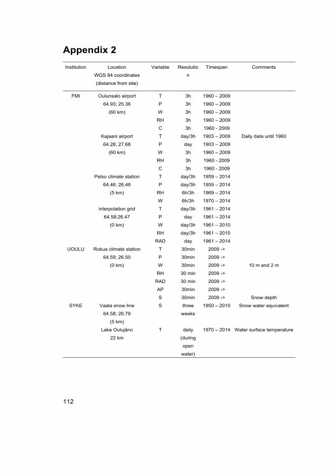
112

Appendix 2

Institution Location

WGS 84 coordinates

(distance from site)

Variable Resolutio

n

Timespan Comments

FMI Oulunsalo airport

64.93; 25.36

(60 km)

T 3h 1960 – 2009

P 3h 1960 – 2009

W 3h 1960 – 2009

RH 3h 1960 – 2009

C 3h 1960 - 2009

Kajaani airport

64.28; 27.68

(60 km)

T day/3h 1903 – 2009 Daily data until 1960

P day 1903 – 2009

W 3h 1960 – 2009

RH 3h 1960 - 2009

C 3h 1960 - 2009

Pelso climate station

64.46; 26.46

(5 km)

T day/3h 1959 – 2014

P day/3h 1959 – 2014

RH 6h/3h 1969 – 2014

W 6h/3h 1970 – 2014

interpolation grid

64.58;26.47

(0 km)

T day/3h 1961 – 2014

P day 1961 – 2014

W day/3h 1961 – 2010

RH day/3h 1961 – 2010

RAD day 1961 – 2014

UOULU Rokua climate station

64.59; 26.50

(0 km)

T 30min 2009 ->

P 30min 2009 ->

W 30min 2009 -> 10 m and 2 m

RH 30 min 2009 ->

RAD 30 min 2009 ->

AP 30min 2009 ->

S 30min 2009 -> Snow depth

SYKE Vaala snow line

64.58; 26.79

(5 km)

S three

weeks

1950 – 2010

Snow water equivalent

Lake Oulujärvi

22 km

T daily

(during

open

water)

1970 – 2014

Water surface temperature

113

Original publications

I Ala-aho P, Rossi, PM & Kløve, B (2013) Interaction of esker groundwater with headwater lakes and streams. Journal of Hydrology 500(2013): 144-156.

II Rossi PM, Ala-aho P, Ronkanen A-K & Kløve B (2012) Groundwater-surface water interaction between an esker aquifer and a drained fen. Journal of Hydrology 432-433 (2012): 52-60.

III Ala-aho P, Rossi, PM & Kløve, B (2014) Estimation of temporal and spatial variations in groundwater recharge in unconfined sand aquifers using scots pine inventories. Hydrology and Earth System Sciences Discussions 11: 7773-7826. (Manuscript)

IV Ala-aho P, Rossi, PM, Isokangas E & Kløve, B (2014) Fully integrated surface-subsurface flow modelling of groundwater-lake interaction in an esker aquifer: Model verification with stable isotopes and airborne thermal imaging. (Manuscript)

Reprinted with permission from Elsevier (I and II) and CC BY 3.0 licence (III).

Original publications are not included in the electronic version of the dissertation.

114

A C T A U N I V E R S I T A T I S O U L U E N S I S

Book orders:Granum: Virtual book storehttp://granum.uta.fi/granum/

S E R I E S C T E C H N I C A

493. Juntunen, Jouni (2014) Enhancing organizational ambidexterity of the FinnishDefence Forces’ supply chain management

494. Hänninen, Kai (2014) Rapid productisation process : managing an unexpectedproduct increment

495. Mehtonen, Saara (2014) The behavior of stabilized high-chromium ferriticstainless steels in hot deformation

496. Majava, Jukka (2014) Product development : drivers, stakeholders, and customerrepresentation during early development

497. Myllylä, Teemu (2014) Multimodal biomedical measurement methods to studybrain functions simultaneously with functional magnetic resonance imaging

498. Tamminen, Satu (2014) Modelling the rejection probability of a quality testconsisting of multiple measurements

499. Tuovinen, Lauri (2014) From machine learning to learning with machines :remodeling the knowledge discovery process

500. Hosio, Simo (2014) Leveraging Social Networking Services on MultipurposePublic Displays

501. Ohenoja, Katja (2014) Particle size distribution and suspension stability inaqueous submicron grinding of CaCO3 and TiO2

502. Puustinen, Jarkko (2014) Phase structure and surface morphology effects on theoptical properties of nanocrystalline PZT thin films

503. Tuhkala, Marko (2014) Dielectric characterization of powdery substances usingan indirectly coupled open-ended coaxial cavity resonator

504. Rezazadegan Tavakoli, Hamed (2014) Visual saliency and eye movement :modeling and applications

505. Tuovinen, Tommi (2014) Operation of IR-UWB WBAN antennas close to humantissues

506. Vasikainen, Soili (2014) Performance management of the university educationprocess

507. Jurmu, Marko (2014) Towards engaging multipurpose public displays : designspace and case studies

509. Huang, Xiaohua (2014) Methods for facial expression recognition withapplications in challenging situations

C510etukansi.kesken.fm Page 2 Thursday, October 30, 2014 3:11 PM

ABCDEFG

UNIVERSITY OF OULU P .O. B 00 F I -90014 UNIVERSITY OF OULU FINLAND

A C T A U N I V E R S I T A T I S O U L U E N S I S

S E R I E S E D I T O R S

SCIENTIAE RERUM NATURALIUM

HUMANIORA

TECHNICA

MEDICA

SCIENTIAE RERUM SOCIALIUM

SCRIPTA ACADEMICA

OECONOMICA

EDITOR IN CHIEF

PUBLICATIONS EDITOR

Professor Esa Hohtola

University Lecturer Santeri Palviainen

Postdoctoral research fellow Sanna Taskila

Professor Olli Vuolteenaho

University Lecturer Veli-Matti Ulvinen

Director Sinikka Eskelinen

Professor Jari Juga

Professor Olli Vuolteenaho

Publications Editor Kirsti Nurkkala

ISBN 978-952-62-0657-8 (Paperback)ISBN 978-952-62-0658-5 (PDF)ISSN 0355-3213 (Print)ISSN 1796-2226 (Online)

U N I V E R S I TAT I S O U L U E N S I SACTAC

TECHNICA

U N I V E R S I TAT I S O U L U E N S I SACTAC

TECHNICA

OULU 2014

C 510

Pertti Ala-aho

GROUNDWATER-SURFACE WATER INTERACTIONS IN ESKER AQUIFERSFROM FIELD MEASUREMENTS TO FULLY INTEGRATED NUMERICAL MODELLING

UNIVERSITY OF OULU GRADUATE SCHOOL;UNIVERSITY OF OULU,FACULTY OF TECHNOLOGY

C 510

ACTA

Pertti Ala-aho

C510etukansi.kesken.fm Page 1 Thursday, October 30, 2014 3:11 PM