O'Sullivan Sheffrin Peres 6e - wps.prenhall.comwps.prenhall.com/wps/media/objects/7538/7719744/PPT/PPT_PDFs/OSP6e... · 6/5/2009 7 Copyright © 2010 Pearson Education, Inc. Publishing

6/5/2009

1

Copyright © 2010 Pearson Education, Inc. Publishing as Prentice Hall.

Econom

ics: P

rincip

les, A

pplications, and T

ools

O

’Sulliv

an,

Sheffri

n,

Pere

z

6/e

.

1 of 37


Econom

ics: P

rincip

les, A

pplications, and T

ools

O

’Sulliv

an,

Sheffri

n,

Pere

z

6/e

.

2 of 37


Econom

ics: P

rincip

les, A

pplications, and T

ools

O

’Sulliv

an,

Sheffri

n,

Pere

z

6/e

.

3 of 37

Perfect Competition

FERNANDO QUIJANO, YVONN QUIJANO,

AND XIAO XUAN XU

P R E P A R E D B Y

Between 2000 and

2006, housing prices

in the United States

increased by about

60 percent.

Econom

ics: P

rincip

les, A

pplications, and T

ools

O

’Sulliv

an,

Sheffri

n,

Pere

z

6/e

.

6/5/2009

2


Econom

ics: P

rincip

les, A

pplications, and T

ools

O

’Sulliv

an,

Sheffri

n,

Pere

z

6/e

.

4 of 38

C H A P T E R 24

Perfect Competition

A P P L Y I N G T H E C O N C E P T S

1

2

3

What is the break-even price?

The Break-Even Price for a Corn Farmer

How do entry costs affect the number of firms in a market?

Wireless Women in Pakistan

How do producers respond to an increase in price?

Wolfram Miners Obey the Law of Supply

Why is the market supply curve positively sloped?

The Worldwide Supply of Copper

How do supply restrictions affect the boom-bust housing

cycle?

Planning Controls and Housing Cycles in Britain

4

5


Econom

ics: P

rincip

les, A

pplications, and T

ools

O

’Sulliv

an,

Sheffri

n,

Pere

z

6/e

.

5 of 38

C H A P T E R 24

Perfect Competition

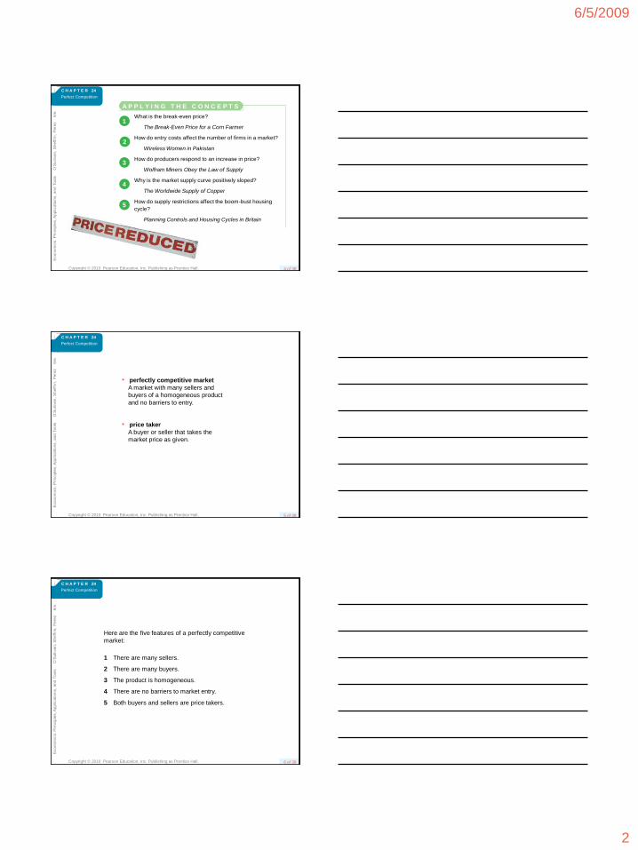
• perfectly competitive market

A market with many sellers and

buyers of a homogeneous product

and no barriers to entry.

• price taker

A buyer or seller that takes the

market price as given.


Econom

ics: P

rincip

les, A

pplications, and T

ools

O

’Sulliv

an,

Sheffri

n,

Pere

z

6/e

.

6 of 38

C H A P T E R 24

Perfect Competition

Here are the five features of a perfectly competitive

market:

1 There are many sellers.

2 There are many buyers.

3 The product is homogeneous.

4 There are no barriers to market entry.

5 Both buyers and sellers are price takers.

6/5/2009

3


Econom

ics: P

rincip

les, A

pplications, and T

ools

O

’Sulliv

an,

Sheffri

n,

Pere

z

6/e

.

7 of 38

C H A P T E R 24

Perfect Competition

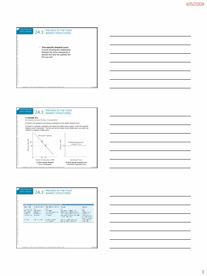
• firm-specific demand curve

A curve showing the relationship

between the price charged by a

specific firm and the quantity the

firm can sell.

PREVIEW OF THE FOUR

MARKET STRUCTURES24.1


Econom

ics: P

rincip

les, A

pplications, and T

ools

O

’Sulliv

an,

Sheffri

n,

Pere

z

6/e

.

8 of 38

C H A P T E R 24

Perfect Competition

FIGURE 24.1

Monopoly versus Perfect Competition

PREVIEW OF THE FOUR


In Panel A, the demand curve facing a monopolist is the market demand curve.

In Panel B, a perfectly competitive firm takes the market price as given, so the firm-specific

demand curve is horizontal. The firm can sell all it wants at the market price, but would sell

nothing if it charged a higher price.


Econom

ics: P

rincip

les, A

pplications, and T

ools

O

’Sulliv

an,

Sheffri

n,

Pere

z

6/e

.

9 of 38

C H A P T E R 24

Perfect CompetitionPREVIEW OF THE FOUR


6/5/2009

4


Econom

ics: P

rincip

les, A

pplications, and T

ools

O

’Sulliv

an,

Sheffri

n,

Pere

z

6/e

.

10 of 38

C H A P T E R 24

Perfect Competition

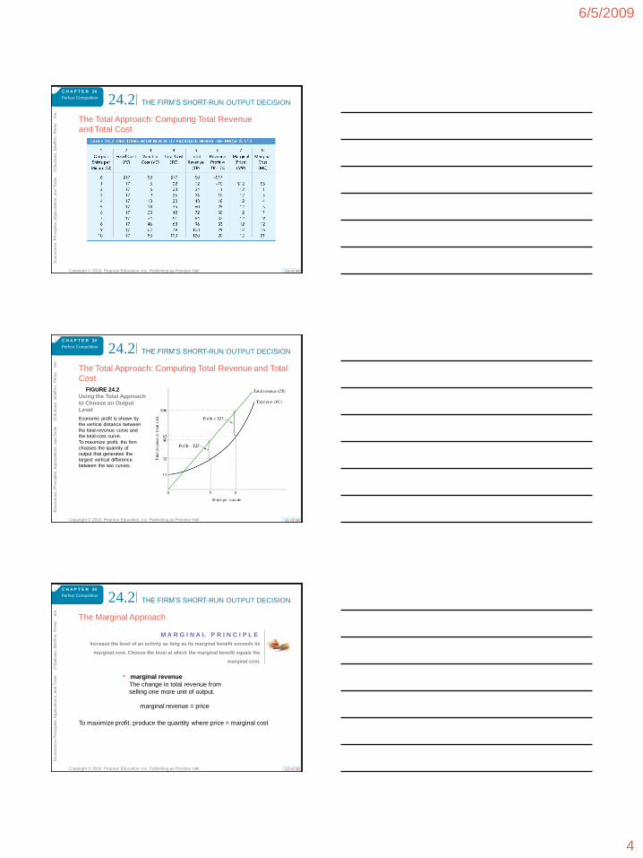
The Total Approach: Computing Total Revenue

and Total Cost

THE FIRM’S SHORT-RUN OUTPUT DECISION24.2


Econom

ics: P

rincip

les, A

pplications, and T

ools

O

’Sulliv

an,

Sheffri

n,

Pere

z

6/e

.

11 of 38

C H A P T E R 24

Perfect Competition

The Total Approach: Computing Total Revenue and Total

Cost

FIGURE 24.2

Using the Total Approach

to Choose an Output

Level

Economic profit is shown by

the vertical distance between

the total-revenue curve and

the total-cost curve.

To maximize profit, the firm

chooses the quantity of

output that generates the

largest vertical difference

between the two curves.



Econom

ics: P

rincip

les, A

pplications, and T

ools

O

’Sulliv

an,

Sheffri

n,

Pere

z

6/e

.

12 of 38

C H A P T E R 24

Perfect Competition

The Marginal Approach

• marginal revenue

The change in total revenue from

selling one more unit of output.

marginal revenue = price

To maximize profit, produce the quantity where price = marginal cost


M A R G I N A L P R I N C I P L E

Increase the level of an activity as long as its marginal benefit exceeds its

marginal cost. Choose the level at which the marginal benefit equals the

marginal cost.

6/5/2009

5


Econom

ics: P

rincip

les, A

pplications, and T

ools

O

’Sulliv

an,

Sheffri

n,

Pere

z

6/e

.

13 of 38

C H A P T E R 24

Perfect Competition

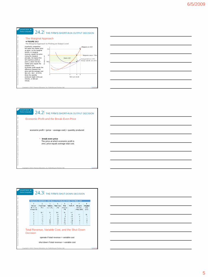
The Marginal Approach FIGURE 24.3

The Marginal Approach to Picking an Output Level

A perfectly competitive

firm takes the market price

as given, so the marginal

benefit, or marginal

revenue, equals the price.

Using the marginal

principle, the typical firm

will maximize profit at

point a, where the $12

market price equals the

marginal cost.

Economic profit equals the

difference between the

price and the average cost

($4.125 = $12 – $7.875)

times the quantity

produced (eight shirts per

minute), or $33 per

minute.



Econom

ics: P

rincip

les, A

pplications, and T

ools

O

’Sulliv

an,

Sheffri

n,

Pere

z

6/e

.

14 of 38

C H A P T E R 24

Perfect Competition

Economic Profit and the Break-Even Price

economic profit = (price − average cost) × quantity produced

• break-even price

The price at which economic profit is

zero; price equals average total cost.



Econom

ics: P

rincip

les, A

pplications, and T

ools

O

’Sulliv

an,

Sheffri

n,

Pere

z

6/e

.

15 of 38

C H A P T E R 24

Perfect Competition

Total Revenue, Variable Cost, and the Shut-Down

Decision

operate if total revenue > variable cost

shut down if total revenue < variable cost

THE FIRM’S SHUT-DOWN DECISION24.3

6/5/2009

6


Econom

ics: P

rincip

les, A

pplications, and T

ools

O

’Sulliv

an,

Sheffri

n,

Pere

z

6/e

.

16 of 38

C H A P T E R 24

Perfect Competition

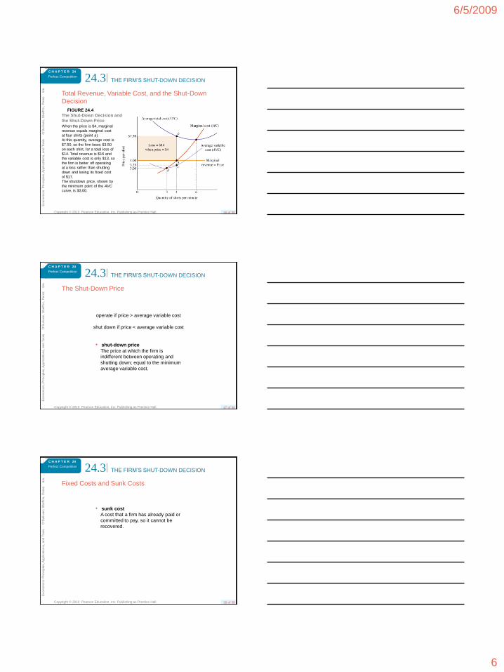
Total Revenue, Variable Cost, and the Shut-Down

Decision

FIGURE 24.4

The Shut-Down Decision and

the Shut-Down Price

When the price is $4, marginal

revenue equals marginal cost

at four shirts (point a).

At this quantity, average cost is

$7.50, so the firm loses $3.50

on each shirt, for a total loss of

$14. Total revenue is $16 and

the variable cost is only $13, so

the firm is better off operating

at a loss rather than shutting

down and losing its fixed cost

of $17.

The shutdown price, shown by

the minimum point of the AVC

curve, is $3.00.



Econom

ics: P

rincip

les, A

pplications, and T

ools

O

’Sulliv

an,

Sheffri

n,

Pere

z

6/e

.

17 of 38

C H A P T E R 24

Perfect Competition

The Shut-Down Price

operate if price > average variable cost

shut down if price < average variable cost

• shut-down price

The price at which the firm is

indifferent between operating and

shutting down; equal to the minimum

average variable cost.



Econom

ics: P

rincip

les, A

pplications, and T

ools

O

’Sulliv

an,

Sheffri

n,

Pere

z

6/e

.

18 of 38

C H A P T E R 24

Perfect Competition

Fixed Costs and Sunk Costs

• sunk cost

A cost that a firm has already paid or

committed to pay, so it cannot be

recovered.


6/5/2009

7


Econom

ics: P

rincip

les, A

pplications, and T

ools

O

’Sulliv

an,

Sheffri

n,

Pere

z

6/e

.

19 of 38

C H A P T E R 24

Perfect Competition

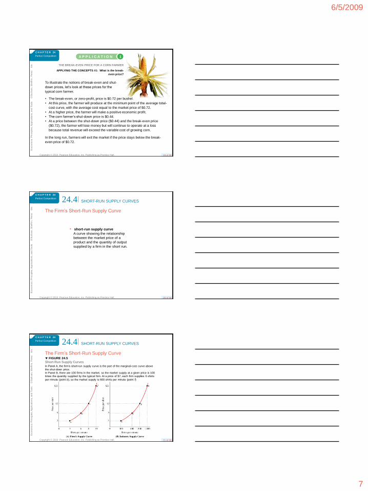
THE BREAK-EVEN PRICE FOR A CORN FARMER

APPLYING THE CONCEPTS #1: What is the break-

even price?

To illustrate the notions of break-even and shut-

down prices, let’s look at these prices for the

typical corn farmer.

• The break-even, or zero-profit, price is $0.72 per bushel.

• At this price, the farmer will produce at the minimum point of the average total-

cost curve, with the average cost equal to the market price of $0.72.

• At a higher price, the farmer will make a positive economic profit.

• The corn farmer’s shut-down price is $0.44.

• At a price between the shut-down price ($0.44) and the break-even price

($0.72), the farmer will lose money but will continue to operate at a loss

because total revenue will exceed the variable cost of growing corn.

In the long run, farmers will exit the market if the price stays below the break-

even price of $0.72.

A P P L I C A T I O N 1


Econom

ics: P

rincip

les, A

pplications, and T

ools

O

’Sulliv

an,

Sheffri

n,

Pere

z

6/e

.

20 of 38

C H A P T E R 24

Perfect Competition

The Firm’s Short-Run Supply Curve

• short-run supply curve


between the market price of a

product and the quantity of output

supplied by a firm in the short run.

SHORT-RUN SUPPLY CURVES24.4


Econom

ics: P

rincip

les, A

pplications, and T

ools

O

’Sulliv

an,

Sheffri

n,

Pere

z

6/e

.

21 of 38

C H A P T E R 24

Perfect Competition

The Firm’s Short-Run Supply Curve FIGURE 24.5

Short-Run Supply Curves


In Panel A, the firm’s short-run supply curve is the part of the marginal-cost curve above

the shut-down price.

In Panel B, there are 100 firms in the market, so the market supply at a given price is 100

times the quantity supplied by the typical firm. At a price of $7, each firm supplies 6 shirts

per minute (point b), so the market supply is 600 shirts per minute (point f)

6/5/2009

8


Econom

ics: P

rincip

les, A

pplications, and T

ools

O

’Sulliv

an,

Sheffri

n,

Pere

z

6/e

.

22 of 38

C H A P T E R 24

Perfect Competition

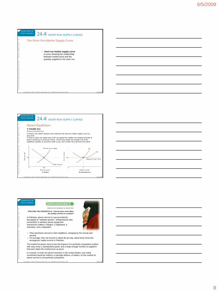
The Short-Run Market Supply Curve

• short-run market supply curve


between market price and the

quantity supplied in the short run.



Econom

ics: P

rincip

les, A

pplications, and T

ools

O

’Sulliv

an,

Sheffri

n,

Pere

z

6/e

.

23 of 38

C H A P T E R 24

Perfect Competition

Market Equilibrium FIGURE 24.6

Market Equilibrium

In Panel A, the market demand curve intersects the short-run market supply curve at a

price of $7.

In Panel B, given the market price of $7, the typical firm satisfies the marginal principle at

point b, producing six shirts per minute. The $7 price equals the average cost at the

equilibrium quantity, so economic profit is zero, and no other firms will enter the market.



Econom

ics: P

rincip

les, A

pplications, and T

ools

O

’Sulliv

an,

Sheffri

n,

Pere

z

6/e

.

24 of 38

C H A P T E R 24

Perfect Competition

WIRELESS WOMEN IN PAKISTAN

APPLYING THE CONCEPTS #2: How do entry costs affect

the number of firms in a market?

In Pakistan, phone service is now provided by

thousands of ―wireless women,‖ entrepreneurs who

invest $310 in wireless phone equipment

(transceiver, battery, charger), a signboard, a

calculator, and a stopwatch.

• They sell phone service to their neighbors, charging by the minute and

second.

• On average, their net income is about $2 per day, about three times the

average per capita income in Pakistan.

The market for phone service has the features of a perfectly competitive market,

with easy entry, a standardized good, and a large enough number of suppliers

that each takes the market price as given.

In contrast, to enter the phone business in the United States, your initial

investment would be millions, or perhaps billions, of dollars, so the market for

phone service is not perfectly competitive.


6/5/2009

9


Econom

ics: P

rincip

les, A

pplications, and T

ools

O

’Sulliv

an,

Sheffri

n,

Pere

z

6/e

.

25 of 38

C H A P T E R 24

Perfect Competition

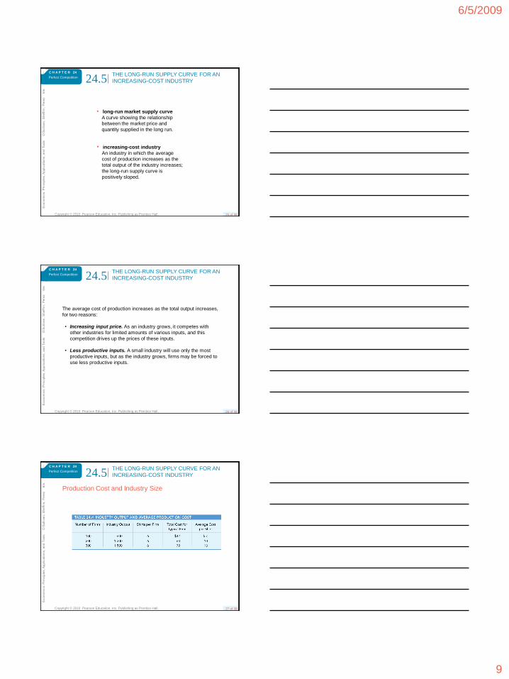
• long-run market supply curve


between the market price and

quantity supplied in the long run.

• increasing-cost industry

An industry in which the average

cost of production increases as the

total output of the industry increases;

the long-run supply curve is

positively sloped.

THE LONG-RUN SUPPLY CURVE FOR AN

INCREASING-COST INDUSTRY24.5


Econom

ics: P

rincip

les, A

pplications, and T

ools

O

’Sulliv

an,

Sheffri

n,

Pere

z

6/e

.

26 of 38

C H A P T E R 24

Perfect Competition

The average cost of production increases as the total output increases,

for two reasons:

• Increasing input price. As an industry grows, it competes with

other industries for limited amounts of various inputs, and this

competition drives up the prices of these inputs.

• Less productive inputs. A small industry will use only the most

productive inputs, but as the industry grows, firms may be forced to

use less productive inputs.




Econom

ics: P

rincip

les, A

pplications, and T

ools

O

’Sulliv

an,

Sheffri

n,

Pere

z

6/e

.

27 of 38

C H A P T E R 24

Perfect Competition

Production Cost and Industry Size



6/5/2009

10


Econom

ics: P

rincip

les, A

pplications, and T

ools

O

’Sulliv

an,

Sheffri

n,

Pere

z

6/e

.

28 of 38

C H A P T E R 24

Perfect Competition

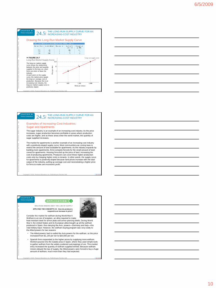
Drawing the Long-Run Market Supply Curve

FIGURE 24.7

Long-Run Market Supply Curve

The long-run market supply

curve shows the relationship

between the price and quantity

supplied in the long run, when

firms can enter or leave the

industry.

At each point on the supply

curve, the market price equals

the long-run average cost of

production. Because this is an

increasing-cost industry, the

long-run market supply curve is

positively sloped.




Econom

ics: P

rincip

les, A

pplications, and T

ools

O

’Sulliv

an,

Sheffri

n,

Pere

z

6/e

.

29 of 38

C H A P T E R 24

Perfect Competition

Examples of Increasing-Cost Industries:

Sugar and Apartments



The sugar industry is an example of an increasing-cost industry. As the price

increases, sugar production becomes profitable in areas where production

costs are higher, and as these areas enter the world market, the quantity of

sugar supplied increases.

The market for apartments is another example of an increasing-cost industry

with a positively sloped supply curve. Most communities use zoning laws to restrict the amount of land available for apartments. As the industry expands by

building more apartments, firms compete fiercely for the small amount of land

zoned for apartments. Housing firms bid up the price of land, increasing the

cost of producing apartments. Producers can cover these higher production

costs only by charging higher rents to tenants. In other words, the supply curve

for apartments is positively sloped because land prices increase with the total

output of the industry, pulling up average cost and necessitating a higher price

for firms to make zero economic profit.


Econom

ics: P

rincip

les, A

pplications, and T

ools

O

’Sulliv

an,

Sheffri

n,

Pere

z

6/e

.

30 of 38

C H A P T E R 24

Perfect Competition

WOLFRAM MINERS OBEY THE LAW OF SUPPLY

APPLYING THE CONCEPTS #3: How do producers

respond to an increase in price?

Consider the market for wolfram during World War II.

Wolfram is an ore of tungsten, an alloy required to make

heat-resistant steel for armor plate and armor-piercing shells. During World

War II, the United States and its European allies bought up all the wolfram

produced in Spain, thus denying the Axis powers—Germany and Italy—this

vital military input. However, the wolfram-buying program was very costly to

the Allied powers for two reasons:

• The Allied powers had to outbid the Axis powers for the wolfram, so the price

increased from $1,144 per ton to $20,000 per ton.

• Spanish firms responded to the higher prices by supplying more wolfram. Workers poured into the Galatia area in Spain, where they used simple tools

to gather wolfram from the widely scattered outcroppings of ore. This market

entry increased the quantity of wolfram supplied tenfold. Because wolfram

miners obeyed the law of supply, the Allied powers were forced to buy a huge

amount of wolfram, much more than they had expected.


6/5/2009

11


Econom

ics: P

rincip

les, A

pplications, and T

ools

O

’Sulliv

an,

Sheffri

n,

Pere

z

6/e

.

31 of 38

C H A P T E R 24

Perfect Competition

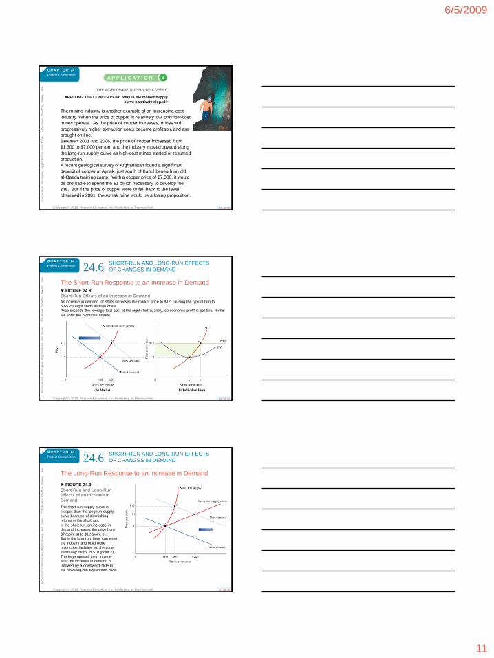
The mining industry is another example of an increasing-cost

industry. When the price of copper is relatively low, only low-cost

mines operate. As the price of copper increases, mines with

progressively higher extraction costs become profitable and are

brought on line.

Between 2001 and 2006, the price of copper increased from

$1,300 to $7,000 per ton, and the industry moved upward along

the long-run supply curve as high-cost mines started or resumed

production.

A recent geological survey of Afghanistan found a significant

deposit of copper at Aynak, just south of Kabul beneath an old

al-Qaeda training camp. With a copper price of $7,000, it would

be profitable to spend the $1 billion necessary to develop the

site. But if the price of copper were to fall back to the level

observed in 2001, the Aynak mine would be a losing proposition.

THE WORLDWIDE SUPPLY OF COPPER

APPLYING THE CONCEPTS #4: Why is the market supply

curve positively sloped?



Econom

ics: P

rincip

les, A

pplications, and T

ools

O

’Sulliv

an,

Sheffri

n,

Pere

z

6/e

.

32 of 38

C H A P T E R 24

Perfect Competition

The Short-Run Response to an Increase in Demand FIGURE 24.8

Short-Run Effects of an Increase in Demand

An increase in demand for shirts increases the market price to $12, causing the typical firm to

produce eight shirts instead of six.

Price exceeds the average total cost at the eight-shirt quantity, so economic profit is positive. Firms

will enter the profitable market.

SHORT-RUN AND LONG-RUN EFFECTS

OF CHANGES IN DEMAND24.6


Econom

ics: P

rincip

les, A

pplications, and T

ools

O

’Sulliv

an,

Sheffri

n,

Pere

z

6/e

.

33 of 38

C H A P T E R 24

Perfect Competition

The Long-Run Response to an Increase in Demand

FIGURE 24.9

Short-Run and Long-Run

Effects of an Increase in

Demand

The short-run supply curve is

steeper than the long-run supply

curve because of diminishing

returns in the short run.

In the short run, an increase in

demand increases the price from

$7 (point a) to $12 (point b).

But in the long run, firms can enter

the industry and build more

production facilities, so the price

eventually drops to $10 (point c).

The large upward jump in price

after the increase in demand is

followed by a downward slide to

the new long-run equilibrium price.

SHORT-RUN AND LONG-RUN EFFECTS

OF CHANGES IN DEMAND24.6

6/5/2009

12


Econom

ics: P

rincip

les, A

pplications, and T

ools

O

’Sulliv

an,

Sheffri

n,

Pere

z

6/e

.

34 of 38

C H A P T E R 24

Perfect Competition

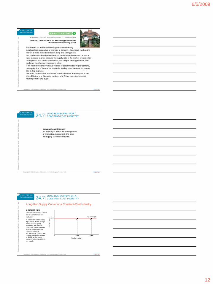
Restrictions on residential development make housing

suppliers less responsive to changes in demand. As a result, the housing

market is more prone to cycles of rising and falling prices.

In a market with development controls, an increase in demand causes a

large increase in price because the supply side of the market is hobbled in

its response. The stricter the controls, the steeper the supply curve, and

the larger the short-run increase in price.

If the restrictions are eventually relaxed to accommodate higher demand,

the supply side of the market responds, leading to an increase in quantity

and a drop in prices.

In Britain, development restrictions are more severe than they are in the

United States, and this partly explains why Britain has more frequent

housing booms and busts.

PLANNING CONTROLS AND HOUSING CYCLES IN BRITAIN

APPLYING THE CONCEPTS #5: How do supply restrictions

affect the boom-bust housing cycle?



Econom

ics: P

rincip

les, A

pplications, and T

ools

O

’Sulliv

an,

Sheffri

n,

Pere

z

6/e

.

35 of 38

C H A P T E R 24

Perfect Competition

• constant-cost industry

An industry in which the average cost

of production is constant; the long-

run supply curve is horizontal.

LONG-RUN SUPPLY FOR A

CONSTANT-COST INDUSTRY24.7


Econom

ics: P

rincip

les, A

pplications, and T

ools

O

’Sulliv

an,

Sheffri

n,

Pere

z

6/e

.

36 of 38

C H A P T E R 24

Perfect Competition

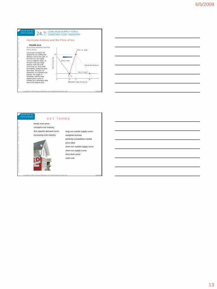
Long-Run Supply Curve for a Constant-Cost Industry

FIGURE 24.10

Long-Run Supply Curve

for a Constant-Cost

Industry

In a constant-cost industry,

input prices do not change

as the industry grows.

Therefore, the average

production cost is constant

and the long-run supply

curve is horizontal.

For the candle industry, the

cost per candle is constant

at $0.05, so the supply

curve is horizontal at $0.05

per candle.



6/5/2009

13


Econom

ics: P

rincip

les, A

pplications, and T

ools

O

’Sulliv

an,

Sheffri

n,

Pere

z

6/e

.

37 of 38

C H A P T E R 24

Perfect Competition

Hurricane Andrew and the Price of Ice

FIGURE 24.11

Hurricane Andrew and the

Price of Ice

A hurricane increases the

demand for ice, shifting the

demand curve to the right. In

the short run, the supply

curve is relatively steep, so

the price rises by a large

amount—from $1 to $5.

In the long run, firms enter

the industry, pulling the price

back down. Because ice

production is a constant-cost

industry, the supply is

horizontal, and the large

upward jump in price is

followed by a downward slide

back to the original price.




Econom

ics: P

rincip

les, A

pplications, and T

ools

O

’Sulliv

an,

Sheffri

n,

Pere

z

6/e

.

38 of 38

C H A P T E R 24

Perfect Competition

break-even price

constant-cost industry

firm-specific demand curve

increasing-cost industry

long-run market supply curve

marginal revenue

perfectly competitive market

price taker

short-run market supply curve

short-run supply curve

shut-down price

sunk cost

K E Y T E R M S

Documents

O'Sullivan Sheffrin Peres 6e - wps.prenhall.comwps.prenhall.com/wps/media/objects/7538/7719744/PPT/PPT_PDFs/OSP6e... · 6/5/2009 7 Copyright © 2010 Pearson Education, Inc. Publishing