Embed Size (px)
Citation preview

Oscilloscope Fundamentals
03W-8605-4_edu.qxd 3/31/09 1:55 PM Page 1
Oscilloscope Fundamentals
2 www.tektronix.com
Table of Contents
Introduction . . . . . . . . . . . . . . . . . . . . . . . . . . . . . . . . . 4
Signal Integrity . . . . . . . . . . . . . . . . . . . . . . . . . . . . 5 - 6
The Significance of Signal Integrity . . . . . . . . . . . . . . . . 5Why is Signal Integrity a Problem? . . . . . . . . . . . . . . . . . 5Viewing the Analog Orgins of Digital Signals . . . . . . . . . 6
The Oscilloscope . . . . . . . . . . . . . . . . . . . . . . . . . 7 - 11
Understanding Waveforms & Waveform Measurements . .7Types of Waves . . . . . . . . . . . . . . . . . . . . . . . . . . . . . . . 8
Sine Waves . . . . . . . . . . . . . . . . . . . . . . . . . . . . . . . . 9Square and Rectangular Waves . . . . . . . . . . . . . . . . 9Sawtooth and Triangle Waves . . . . . . . . . . . . . . . . . 9Step and Pulse Shapes . . . . . . . . . . . . . . . . . . . . . . 9Periodic and Non-periodic Signals . . . . . . . . . . . . . 10Synchronous and Asynchronous Signals . . . . . . . . 10Complex Waves . . . . . . . . . . . . . . . . . . . . . . . . . . . 10Eye Patterns . . . . . . . . . . . . . . . . . . . . . . . . . . . . . . 10Constellation Diagrams . . . . . . . . . . . . . . . . . . . . . . 11
Waveform Measurements . . . . . . . . . . . . . . . . . . . . . . .11Frequency and Period . . . . . . . . . . . . . . . . . . . . . . .11Voltage . . . . . . . . . . . . . . . . . . . . . . . . . . . . . . . . . . 11Amplitude . . . . . . . . . . . . . . . . . . . . . . . . . . . . . . . . 12Phase . . . . . . . . . . . . . . . . . . . . . . . . . . . . . . . . . . 12Waveform Measurements with Digital Oscilloscopes 12
Types of Oscilloscopes . . . . . . . . . . . . . . . . . . . .13 - 17Digital Oscilloscopes . . . . . . . . . . . . . . . . . . . . . . . . . . 13
Digital Storage Oscilloscopes . . . . . . . . . . . . . . . . 14Digital Phosphor Oscilloscopes . . . . . . . . . . . . . . . 15Digital Sampling Oscilloscopes . . . . . . . . . . . . . . . 17
The Systems and Controls of an Oscilloscope .18 - 31
Vertical System and Controls . . . . . . . . . . . . . . . . . . . . 19Position and Volts per Division . . . . . . . . . . . . . . . . 19Input Coupling . . . . . . . . . . . . . . . . . . . . . . . . . . . . 19Bandwidth Limit . . . . . . . . . . . . . . . . . . . . . . . . . . . 19Bandwidth Enhancement . . . . . . . . . . . . . . . . . . . . 20
Horizontal System and Controls . . . . . . . . . . . . . . . . . 20Acquisition Controls . . . . . . . . . . . . . . . . . . . . . . . . 20Acquisition Modes . . . . . . . . . . . . . . . . . . . . . . . . . 20Types of Acquisition Modes . . . . . . . . . . . . . . . . . . 21Starting and Stopping the Acquisition System . . . . 21Sampling . . . . . . . . . . . . . . . . . . . . . . . . . . . . . . . . 22Sampling Controls . . . . . . . . . . . . . . . . . . . . . . . . . 22Sampling Methods . . . . . . . . . . . . . . . . . . . . . . . . 22Real-time Sampling . . . . . . . . . . . . . . . . . . . . . . . . 22
Equivalent-time Sampling . . . . . . . . . . . . . . . . . . 24Position and Seconds per Division . . . . . . . . . . . . . 26Time Base Selections . . . . . . . . . . . . . . . . . . . . . . . 26Zoom . . . . . . . . . . . . . . . . . . . . . . . . . . . . . . . . . . . 26XY Mode . . . . . . . . . . . . . . . . . . . . . . . . . . . . . . . . 26Z Axis . . . . . . . . . . . . . . . . . . . . . . . . . . . . . . . . . . . 26XYZ Mode . . . . . . . . . . . . . . . . . . . . . . . . . . . . . . . 26
Trigger System and Controls . . . . . . . . . . . . . . . . . . . . 27Trigger Position . . . . . . . . . . . . . . . . . . . . . . . . . . . . 28Trigger Level and Slope . . . . . . . . . . . . . . . . . . . . . 28Trigger Sources . . . . . . . . . . . . . . . . . . . . . . . . . . . 28Trigger Modes . . . . . . . . . . . . . . . . . . . . . . . . . . . . 29Trigger Coupling . . . . . . . . . . . . . . . . . . . . . . . . . . . 30Trigger Holdoff . . . . . . . . . . . . . . . . . . . . . . . . . . . . 30
Display System and Controls . . . . . . . . . . . . . . . . . . . . 30Other Oscilloscope Controls . . . . . . . . . . . . . . . . . . . . . 31
Math and Measurement Operations . . . . . . . . . . . . 31
03W-8605-4_edu.qxd 3/31/09 1:55 PM Page 2
Oscilloscope Fundamentals
3www.tektronix.com
The Complete Measurement System . . . . . . . . 32 - 34
Probes . . . . . . . . . . . . . . . . . . . . . . . . . . . . . . . . . . . 32Passive Probes . . . . . . . . . . . . . . . . . . . . . . . . . . . . . . 32Active and Differential Probes . . . . . . . . . . . . . . . . . . . . 33Probe Accessories . . . . . . . . . . . . . . . . . . . . . . . . . . . 34
Performance Terms and Considerations . . . . . 35 - 43
Bandwidth . . . . . . . . . . . . . . . . . . . . . . . . . . . . . . . . . . 35Rise Time . . . . . . . . . . . . . . . . . . . . . . . . . . . . . . . . . . . 36Sample Rate . . . . . . . . . . . . . . . . . . . . . . . . . . . . . . . . 37Waveform Capture Rate . . . . . . . . . . . . . . . . . . . . . . . . 38Record Length . . . . . . . . . . . . . . . . . . . . . . . . . . . . . . . 39Triggering Capabilities . . . . . . . . . . . . . . . . . . . . . . . . . 39Effective Bits . . . . . . . . . . . . . . . . . . . . . . . . . . . . . . . . 39Frequency Response . . . . . . . . . . . . . . . . . . . . . . . . . . 39Vertical Sensitivity . . . . . . . . . . . . . . . . . . . . . . . . . . . . . 39Sweep Speed . . . . . . . . . . . . . . . . . . . . . . . . . . . . . . . 40Gain Accuracy . . . . . . . . . . . . . . . . . . . . . . . . . . . . . . . 40Horizontal Accuracy (Time Base) . . . . . . . . . . . . . . . . . 40Vertical Resolution (Analog-to-digital Converter) . . . . . . 40Connectivity . . . . . . . . . . . . . . . . . . . . . . . . . . . . . . . . . 40Expandability . . . . . . . . . . . . . . . . . . . . . . . . . . . . . . . . 41Ease-of-use . . . . . . . . . . . . . . . . . . . . . . . . . . . . . . . . . 42Probes . . . . . . . . . . . . . . . . . . . . . . . . . . . . . . . . . . . 43
Operating the Oscilloscope . . . . . . . . . . . . . . . . 44 - 46
Setting Up . . . . . . . . . . . . . . . . . . . . . . . . . . . . . . . . . . 44Ground the Oscilloscope . . . . . . . . . . . . . . . . . . . . . . . 44Ground Yourself . . . . . . . . . . . . . . . . . . . . . . . . . . . . . . 44Setting the Controls . . . . . . . . . . . . . . . . . . . . . . . . . . . 44Instrument Calibration . . . . . . . . . . . . . . . . . . . . . . . . . 45Using Probes . . . . . . . . . . . . . . . . . . . . . . . . . . . . . . . . 45Connecting the Ground Clip . . . . . . . . . . . . . . . . . . . . . 45Compensating the Probe . . . . . . . . . . . . . . . . . . . . . . . 46
Oscilloscope Measurement Techniques . . . . . . 47 - 51
Voltage Measurements . . . . . . . . . . . . . . . . . . . . . . . . . 47Time and Frequency Measurements . . . . . . . . . . . . . . 48Pulse Width and Rise Time Measurements . . . . . . . . . 48Phase Shift Measurements . . . . . . . . . . . . . . . . . . . . . . 49Other Measurement Techniques . . . . . . . . . . . . . . . . . . 49
Written Exercises . . . . . . . . . . . . . . . . . . . . . . . . 50 - 55
Part IA. Vocabulary Exercises . . . . . . . . . . . . . . . . . . . . . 50B. Application Exercises . . . . . . . . . . . . . . . . . . . . . 51
Part IIA. Vocabulary Exercises . . . . . . . . . . . . . . . . . . . . . 52B. Application Exercises . . . . . . . . . . . . . . . . . . . . .53
Answer Key . . . . . . . . . . . . . . . . . . . . . . . . . . . . . . . . . .55
Glossary . . . . . . . . . . . . . . . . . . . . . . . . . . . . . . 56 - 59
03W-8605-4_edu.qxd 3/31/09 1:55 PM Page 3
Oscilloscope Fundamentals
IntroductionNature moves in the form of a sine wave, be it an oceanwave, earthquake, sonic boom, explosion, sound through air,or the natural frequency of a body in motion. Energy, vibratingparticles and other invisible forces pervade our physical uni-verse. Even light – part particle, part wave – has a fundamen-tal frequency, which can be observed as color.
Sensors can convert these forces into electricalsignals that you can observe and study with anoscilloscope. Oscilloscopes enable scientists,engineers, technicians, educators and others to“see” events that change over time.
Oscilloscopes are indispensable tools for anyone designing,manufacturing or repairing electronic equipment. In today’sfast-paced world, engineers need the best tools available tosolve their measurement challenges quickly and accurately.As the eyes of the engineer, oscilloscopes are the key tomeeting today’s demanding measurement challenges.
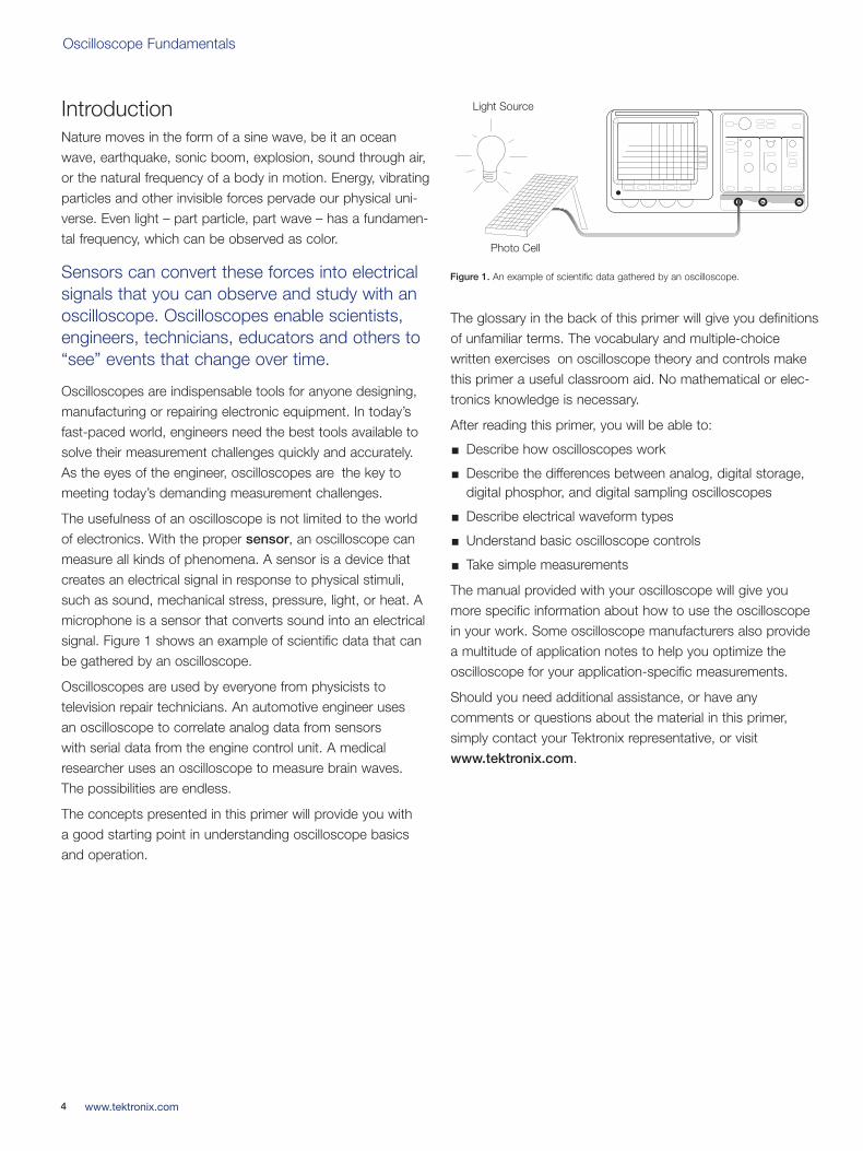
The usefulness of an oscilloscope is not limited to the worldof electronics. With the proper sensor, an oscilloscope canmeasure all kinds of phenomena. A sensor is a device thatcreates an electrical signal in response to physical stimuli,such as sound, mechanical stress, pressure, light, or heat. Amicrophone is a sensor that converts sound into an electricalsignal. Figure 1 shows an example of scientific data that canbe gathered by an oscilloscope.
Oscilloscopes are used by everyone from physicists to television repair technicians. An automotive engineer uses an oscilloscope to correlate analog data from sensors with serial data from the engine control unit. A medicalresearcher uses an oscilloscope to measure brain waves. The possibilities are endless.
The concepts presented in this primer will provide you with a good starting point in understanding oscilloscope basicsand operation.
The glossary in the back of this primer will give you definitionsof unfamiliar terms. The vocabulary and multiple-choice written exercises on oscilloscope theory and controls makethis primer a useful classroom aid. No mathematical or elec-tronics knowledge is necessary.
After reading this primer, you will be able to:
Describe how oscilloscopes work
Describe the differences between analog, digital storage,digital phosphor, and digital sampling oscilloscopes
Describe electrical waveform types
Understand basic oscilloscope controls
Take simple measurements
The manual provided with your oscilloscope will give youmore specific information about how to use the oscilloscopein your work. Some oscilloscope manufacturers also providea multitude of application notes to help you optimize theoscilloscope for your application-specific measurements.
Should you need additional assistance, or have any comments or questions about the material in this primer, simply contact your Tektronix representative, or visit www.tektronix.com.
4 www.tektronix.com
Photo Cell
Light Source
Figure 1. An example of scientific data gathered by an oscilloscope.
03W-8605-4_edu.qxd 3/31/09 1:55 PM Page 4
Oscilloscope Fundamentals
5www.tektronix.com
Signal Integrity
The Significance of Signal Integrity
The key to any good oscilloscope system is its ability toaccurately reconstruct a waveform – referred to as signal
integrity. An oscilloscope is analogous to a camera that captures signal images that we can then observe and interpret. Two key issues lie at the heart of signal integrity.
When you take a picture, is it an accurate picture of whatactually happened?
Is the picture clear or fuzzy?
How many of those accurate pictures can you take persecond?
Taken together, the different systems and performance capa-bilities of an oscilloscope contribute to its ability to deliver thehighest signal integrity possible. Probes also affect the signalintegrity of a measurement system.
Signal integrity impacts many electronic design disciplines.But until a few years ago, it wasn’t much of a problem fordigital designers. They could rely on their logic designs to act like the Boolean circuits they were. Noisy, indeterminatesignals were something that occurred in high-speed designs– something for RF designers to worry about. Digital systemsswitched slowly and signals stabilized predictably.
Processor clock rates have since multiplied by orders ofmagnitude. Computer applications such as 3D graphics,video and server I/O demand vast bandwidth. Much oftoday’s telecommunications equipment is digitally based, and similarly requires massive bandwidth. So too does digital high-definition TV. The current crop of microprocessordevices handles data at rates up to 2, 3 and even 5 GS/s(gigasamples per second), while some DDR3 memorydevices use clocks in excess of 2 GHz as well as data signalswith 35-ps rise times.
Importantly, speed increases have trickled down to the common IC devices used in automobiles, VCRs, andmachine controllers, to name just a few applications.
A processor running at a 20-MHz clock rate may well havesignals with rise times similar to those of an 800-MHzprocessor. Designers have crossed a performance thresholdthat means, in effect, almost every design is a high-speeddesign.
Without some precautionary measures, high-speed problemscan creep into otherwise conventional digital designs. If a circuit is experiencing intermittent failures, or if it encounterserrors at voltage and temperature extremes, chances arethere are some hidden signal integrity problems. These canaffect time-to-market, product reliability, EMI compliance, and more. These high speed problems can also impact theintegrity of a serial data stream in a system, requiring somemethod of correlating specific patterns in the data with theobserved characteristics of high-speed waveforms.
Why is Signal Integrity a Problem?
Let’s look at some of the specific causes of signal degrada-tion in today’s digital designs. Why are these problems somuch more prevalent today than in years past?
The answer is speed. In the “slow old days,” maintainingacceptable digital signal integrity meant paying attention todetails like clock distribution, signal path design, noise mar-gins, loading effects, transmission line effects, bus termina-tion, decoupling and power distribution. All of these rules stillapply, but…
Bus cycle times are up to a thousand times faster than theywere 20 years ago! Transactions that once took microsec-onds are now measured in nanoseconds. To achieve thisimprovement, edge speeds too have accelerated: they are up to 100 times faster than those of two decades ago.
This is all well and good; however, certain physical realitieshave kept circuit board technology from keeping up the pace.The propagation time of inter-chip buses has remainedalmost unchanged over the decades. Geometries haveshrunk, certainly, but there is still a need to provide circuitboard real estate for IC devices, connectors, passive compo-nents, and of course, the bus traces themselves. This realestate adds up to distance, and distance means time – theenemy of speed.
03W-8605-4_edu.qxd 3/31/09 1:55 PM Page 5
Oscilloscope Fundamentals
It’s important to remember that the edge speed – rise time –of a digital signal can carry much higher frequency compo-nents than its repetition rate might imply. For this reason,some designers deliberately seek IC devices with relatively“slow” rise times.
The lumped circuit model has always been the basis of most calculations used to predict signal behavior in a circuit.But when edge speeds are more than four to six times fasterthan the signal path delay, the simple lumped model nolonger applies.
Circuit board traces just six inches long become transmissionlines when driven with signals exhibiting edge rates belowfour to six nanoseconds, irrespective of the cycle rate. In effect, new signal paths are created. These intangible connections aren’t on the schematics, but nevertheless provide a means for signals to influence one another inunpredictable ways.
Sometimes even the errors introduced by theprobe/instrument combination can provide a significant contribution to the signal beingmeasured. However, by applying the “squareroot of the sum of the squares” formula to themeasured value, it is possible to determinewhether the device under test is approaching a rise/fall time failure. In addition, recent oscilloscope tools use special filtering tech-niques to de-embed the measurement system’seffects on the signal, displaying edge times and other signal characteristics.
At the same time, the intended signal paths don’t work theway they are supposed to. Ground planes and power planes,like the signal traces described above, become inductive and act like transmission lines; power supply decoupling is far less effective. EMI goes up as faster edge speeds produce shorter wavelengths relative to the bus length.Crosstalk increases.
In addition, fast edge speeds require generally higher currentsto produce them. Higher currents tend to cause groundbounce, especially on wide buses in which many signalsswitch at once. Moreover, higher current increases theamount of radiated magnetic energy and with it, crosstalk.
Viewing the Analog Origins of Digital Signals
What do all these characteristics have in common? They are classic analog phenomena. To solve signal integrity problems, digital designers need to step into the analogdomain. And to take that step, they need tools that can show them how digital and analog signals interact.
Digital errors often have their roots in analog signal integrityproblems. To track down the cause of the digital fault, it’soften necessary to turn to an oscilloscope, which can displaywaveform details, edges and noise; can detect and displaytransients; and can help you precisely measure timing relationships such as setup and hold times. Modern oscillo-scopes can help to simplify the troubleshooting process bytriggering on specific patterns in serial data streams and displaying the analog signal that corresponds in time with a specified event.
Understanding each of the systems within your oscilloscopeand how to apply them will contribute to the effective application of the oscilloscope to tackle your specific measurement challenge.
6 www.tektronix.com
03W-8605-4_edu.qxd 3/31/09 1:55 PM Page 6
Oscilloscope Fundamentals
7www.tektronix.com
The OscilloscopeWhat is an oscilloscope and how does it work? This sectionanswers these fundamental questions.
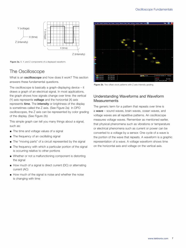
The oscilloscope is basically a graph-displaying device – itdraws a graph of an electrical signal. In most applications,the graph shows how signals change over time: the vertical(Y) axis represents voltage and the horizontal (X) axis represents time. The intensity or brightness of the display is sometimes called the Z axis. (See Figure 2a) In DPO oscilloscopes, the Z axis can be represented by color gradingof the display. (See Figure 2b)
This simple graph can tell you many things about a signal,such as:
The time and voltage values of a signal
The frequency of an oscillating signal
The “moving parts” of a circuit represented by the signal
The frequency with which a particular portion of the signalis occurring relative to other portions
Whether or not a malfunctioning component is distortingthe signal
How much of a signal is direct current (DC) or alternatingcurrent (AC)
How much of the signal is noise and whether the noise is changing with time
Understanding Waveforms and WaveformMeasurements
The generic term for a pattern that repeats over time is a wave – sound waves, brain waves, ocean waves, and voltage waves are all repetitive patterns. An oscilloscopemeasures voltage waves. Remember as mentioned earlier,that physical phenomena such as vibrations or temperatureor electrical phenomena such as current or power can beconverted to a voltage by a sensor. One cycle of a wave isthe portion of the wave that repeats. A waveform is a graphicrepresentation of a wave. A voltage waveform shows time on the horizontal axis and voltage on the vertical axis.
Z (intensity)
Y (voltage)
X (time)
Y (voltage)
X (time)
Z (intensity)
Figure 2a. X, Y, and Z components of a displayed waveform.
Figure 2b. Two offset clock patterns with Z axis intensity grading.
03W-8605-4_edu.qxd 3/31/09 1:55 PM Page 7
Oscilloscope Fundamentals
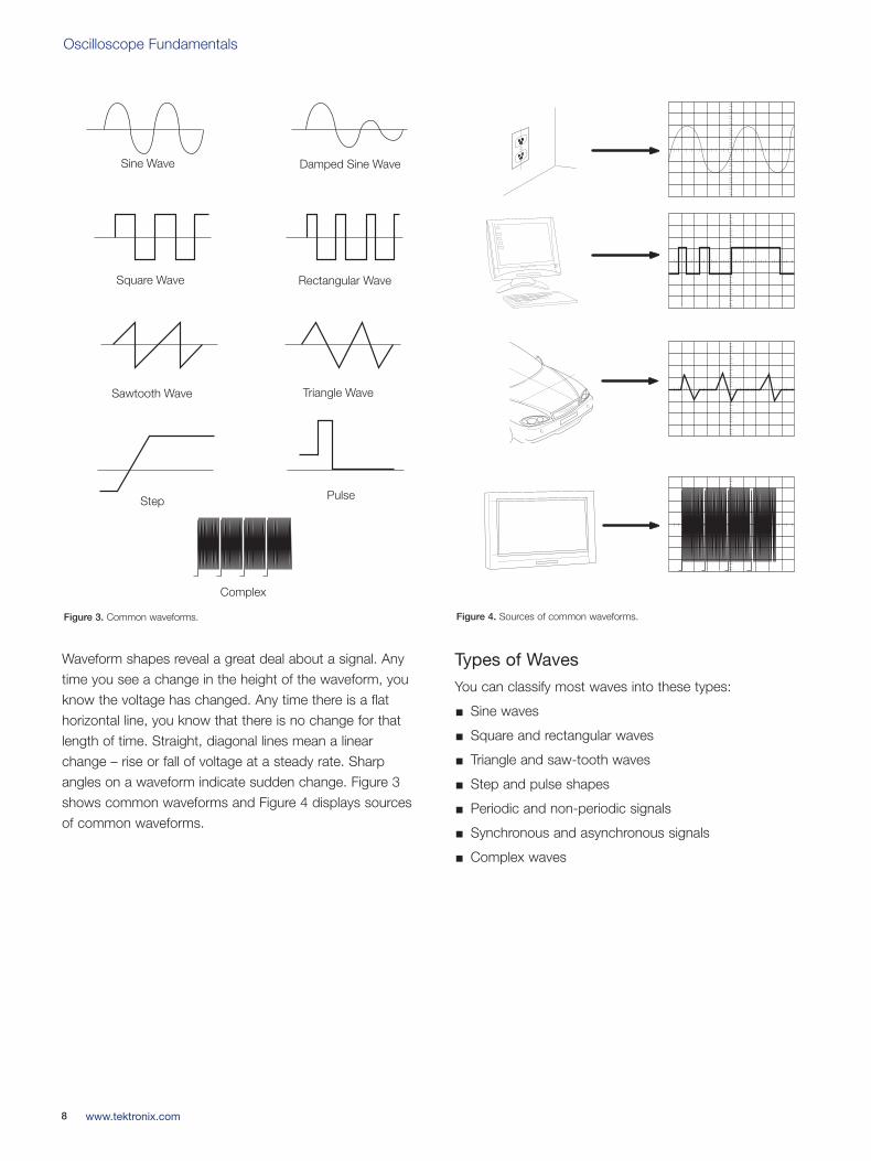
Waveform shapes reveal a great deal about a signal. Any time you see a change in the height of the waveform, youknow the voltage has changed. Any time there is a flat horizontal line, you know that there is no change for thatlength of time. Straight, diagonal lines mean a linear change – rise or fall of voltage at a steady rate. Sharp angles on a waveform indicate sudden change. Figure 3shows common waveforms and Figure 4 displays sources of common waveforms.
Types of Waves
You can classify most waves into these types:
Sine waves
Square and rectangular waves
Triangle and saw-tooth waves
Step and pulse shapes
Periodic and non-periodic signals
Synchronous and asynchronous signals
Complex waves
8 www.tektronix.com
Figure 4. Sources of common waveforms.
Sine Wave Damped Sine Wave
Square Wave Rectangular Wave
Sawtooth Wave Triangle Wave
Step Pulse
Complex
Figure 3. Common waveforms.
03W-8605-4_edu.qxd 3/31/09 1:55 PM Page 8
Oscilloscope Fundamentals
9www.tektronix.com
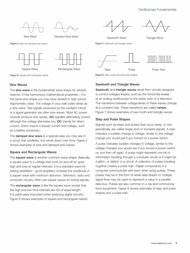
Sine Waves
The sine wave is the fundamental wave shape for several reasons. It has harmonious mathematical properties – it is the same sine shape you may have studied in high schooltrigonometry class. The voltage in your wall outlet varies as a sine wave. Test signals produced by the oscillator circuit of a signal generator are often sine waves. Most AC powersources produce sine waves. (AC signifies alternating current,although the voltage alternates too. DC stands for direct current, which means a steady current and voltage, such as a battery produces.)
The damped sine wave is a special case you may see in a circuit that oscillates, but winds down over time. Figure 5shows examples of sine and damped sine waves.
Square and Rectangular Waves
The square wave is another common wave shape. Basically,a square wave is a voltage that turns on and off (or goes high and low) at regular intervals. It is a standard wave fortesting amplifiers – good amplifiers increase the amplitude ofa square wave with minimum distortion. Television, radio andcomputer circuitry often use square waves for timing signals.
The rectangular wave is like the square wave except that the high and low time intervals are not of equal length. It is particularly important when analyzing digital circuitry.Figure 6 shows examples of square and rectangular waves.
Sawtooth and Triangle Waves
Sawtooth and triangle waves result from circuits designedto control voltages linearly, such as the horizontal sweep of an analog oscilloscope or the raster scan of a television. The transitions between voltage levels of these waves changeat a constant rate. These transitions are called ramps. Figure 7 shows examples of saw-tooth and triangle waves.
Step and Pulse Shapes
Signals such as steps and pulses that occur rarely, or non-periodically, are called single-shot or transient signals. A stepindicates a sudden change in voltage, similar to the voltagechange you would see if you turned on a power switch.
A pulse indicates sudden changes in voltage, similar to thevoltage changes you would see if you turned a power switchon and then off again. A pulse might represent one bit ofinformation traveling through a computer circuit or it might bea glitch, or defect, in a circuit. A collection of pulses travelingtogether creates a pulse train. Digital components in a computer communicate with each other using pulses. Thesepulses may be in the form of serial data stream or multiplesignal lines may be used to represent a value in a paralleldata bus. Pulses are also common in x-ray and communica-tions equipment. Figure 8 shows examples of step and pulseshapes and a pulse train.
Sine Wave Damped Sine Wave
Figure 5. Sine and damped sine waves.
Square Wave Rectangular Wave
Figure 6. Square and rectangular waves.
Step Pulse Pulse Train
Figure 8. Step, pulse and pulse train shapes.
Sawtooth Wave Triangle Wave
Figure 7. Sawtooth and triangle waves.
03W-8605-4_edu.qxd 3/31/09 1:55 PM Page 9
Oscilloscope Fundamentals
Periodic and Non-periodic Signals
Repetitive signals are referred to as periodic signals, whilesignals that constantly change are known as non-periodic
signals. A still picture is analogous to a periodic signal, whilea moving picture can be equated to a non-periodic signal.
Synchronous and Asynchronous Signals
When a timing relationship exists between two signals, those signals are referred to as synchronous. Clock, data and address signals inside a computer are an example ofsynchronous signals.
Asynchronous is a term used to describe those signalsbetween which no timing relationship exists. Because no time correlation exists between the act of touching a key on a computer keyboard and the clock inside the computer,these are considered asynchronous.
Complex Waves
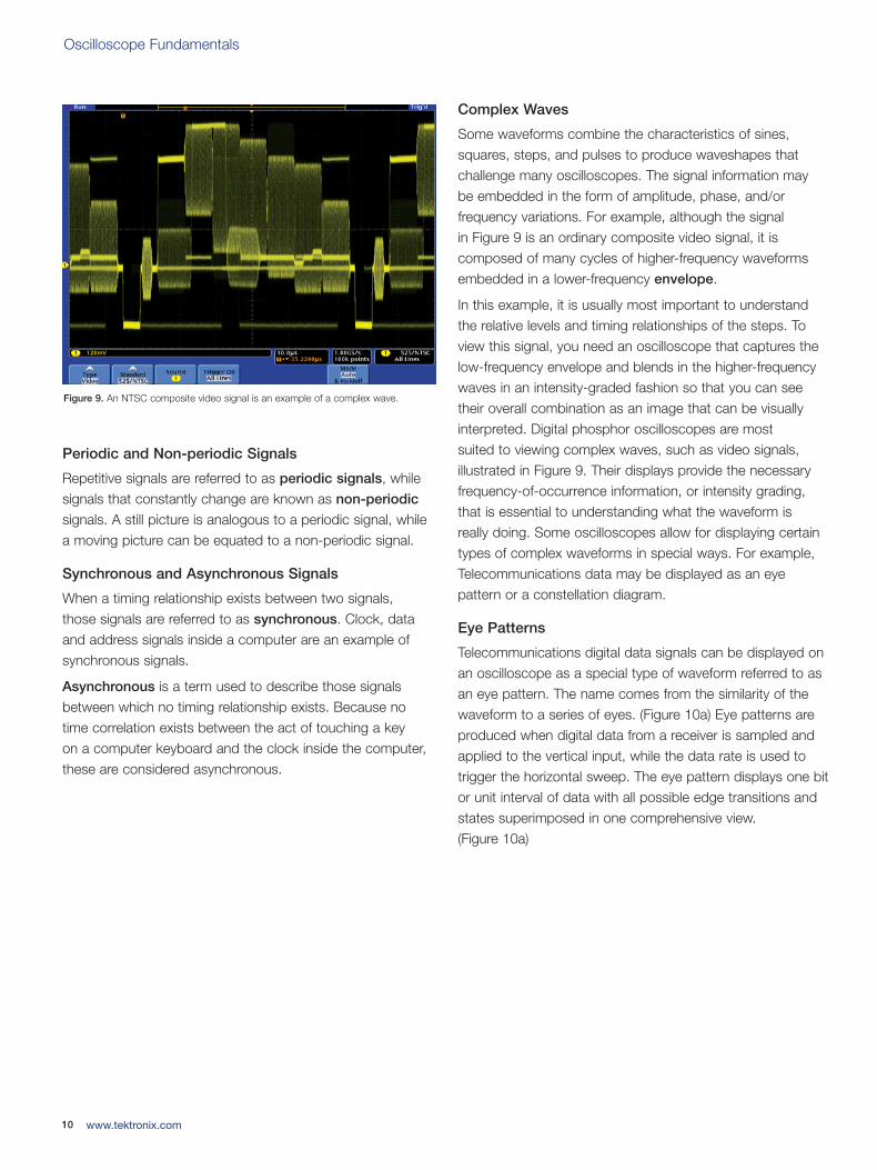
Some waveforms combine the characteristics of sines,squares, steps, and pulses to produce waveshapes thatchallenge many oscilloscopes. The signal information may be embedded in the form of amplitude, phase, and/or frequency variations. For example, although the signal in Figure 9 is an ordinary composite video signal, it is composed of many cycles of higher-frequency waveformsembedded in a lower-frequency envelope.
In this example, it is usually most important to understand the relative levels and timing relationships of the steps. Toview this signal, you need an oscilloscope that captures thelow-frequency envelope and blends in the higher-frequencywaves in an intensity-graded fashion so that you can seetheir overall combination as an image that can be visuallyinterpreted. Digital phosphor oscilloscopes are most suited to viewing complex waves, such as video signals, illustrated in Figure 9. Their displays provide the necessaryfrequency-of-occurrence information, or intensity grading,that is essential to understanding what the waveform is really doing. Some oscilloscopes allow for displaying certain types of complex waveforms in special ways. For example,Telecommunications data may be displayed as an eye pattern or a constellation diagram.
Eye Patterns
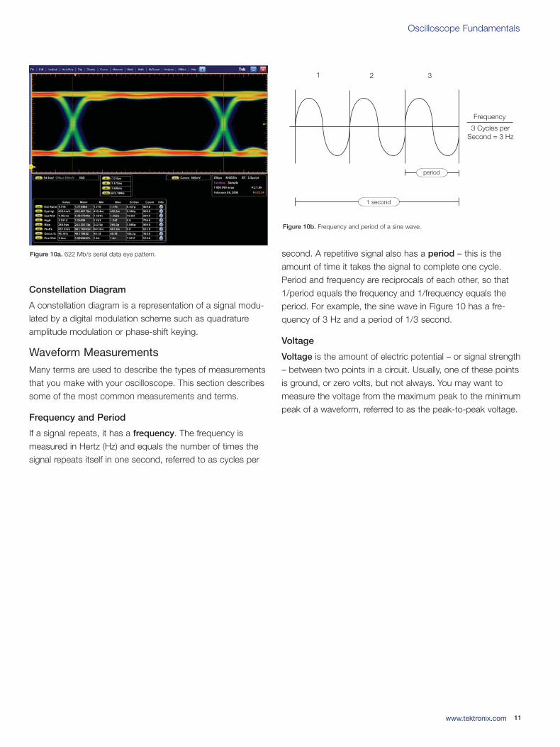
Telecommunications digital data signals can be displayed onan oscilloscope as a special type of waveform referred to asan eye pattern. The name comes from the similarity of thewaveform to a series of eyes. (Figure 10a) Eye patterns areproduced when digital data from a receiver is sampled andapplied to the vertical input, while the data rate is used totrigger the horizontal sweep. The eye pattern displays one bitor unit interval of data with all possible edge transitions andstates superimposed in one comprehensive view. (Figure 10a)
10 www.tektronix.com
Complex
Figure 9. An NTSC composite video signal is an example of a complex wave.
03W-8605-4_edu.qxd 3/31/09 1:55 PM Page 10
Oscilloscope Fundamentals
11www.tektronix.com
Constellation Diagram
A constellation diagram is a representation of a signal modu-lated by a digital modulation scheme such as quadratureamplitude modulation or phase-shift keying.
Waveform Measurements
Many terms are used to describe the types of measurementsthat you make with your oscilloscope. This section describessome of the most common measurements and terms.
Frequency and Period
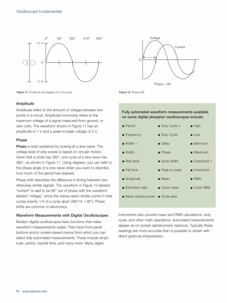
If a signal repeats, it has a frequency. The frequency ismeasured in Hertz (Hz) and equals the number of times thesignal repeats itself in one second, referred to as cycles per
second. A repetitive signal also has a period – this is theamount of time it takes the signal to complete one cycle.Period and frequency are reciprocals of each other, so that1/period equals the frequency and 1/frequency equals theperiod. For example, the sine wave in Figure 10 has a fre-quency of 3 Hz and a period of 1/3 second.
Voltage
Voltage is the amount of electric potential – or signal strength– between two points in a circuit. Usually, one of these pointsis ground, or zero volts, but not always. You may want tomeasure the voltage from the maximum peak to the minimumpeak of a waveform, referred to as the peak-to-peak voltage.
period
1 second
3 Cycles perSecond = 3 Hz
Frequency
1 2 3
Figure 10b. Frequency and period of a sine wave.
Figure 10a. 622 Mb/s serial data eye pattern.
03W-8605-4_edu.qxd 3/31/09 1:55 PM Page 11
Oscilloscope Fundamentals
Amplitude
Amplitude refers to the amount of voltage between twopoints in a circuit. Amplitude commonly refers to the maximum voltage of a signal measured from ground, or zero volts. The waveform shown in Figure 11 has an amplitude of 1 V and a peak-to-peak voltage of 2 V.
Phase
Phase is best explained by looking at a sine wave. The voltage level of sine waves is based on circular motion. Given that a circle has 360°, one cycle of a sine wave has360°, as shown in Figure 11. Using degrees, you can refer tothe phase angle of a sine wave when you want to describehow much of the period has elapsed.
Phase shift describes the difference in timing between twootherwise similar signals. The waveform in Figure 12 labeled“current” is said to be 90° out of phase with the waveformlabeled “voltage,” since the waves reach similar points in theircycles exactly 1/4 of a cycle apart (360°/4 = 90°). Phaseshifts are common in electronics.
Waveform Measurements with Digital Oscilloscopes
Modern digital oscilloscopes have functions that make waveform measurements easier. They have front-panel buttons and/or screen-based menus from which you canselect fully automated measurements. These include ampli-tude, period, rise/fall time, and many more. Many digital
instruments also provide mean and RMS calculations, dutycycle, and other math operations. Automated measurementsappear as on-screen alphanumeric readouts. Typically thesereadings are more accurate than is possible to obtain withdirect graticule interpretation.
12 www.tektronix.com
0° 90° 180° 270° 360+1 V
–1 V
02 V
°
Figure 11. Amplitude and degrees of a sine wave.
0
Phase = 90°
Voltage
Current
Figure 12. Phase shift.
Fully automated waveform measurements available on some digital phosphor oscilloscopes include:
Period Duty Cycle + High
Frequency Duty Cycle - Low
Width + Delay Minimum
Width - Phase Maximum
Rise time Burst width Overshoot +
Fall time Peak-to-peak Overshoot -
Amplitude Mean RMS
Extinction ratio Cycle mean Cycle RMS
Mean optical power Cycle area
03W-8605-4_edu.qxd 3/31/09 1:55 PM Page 12
Oscilloscope Fundamentals
13www.tektronix.com
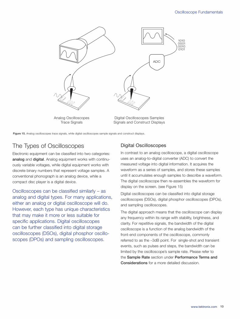
The Types of OscilloscopesElectronic equipment can be classified into two categories:analog and digital. Analog equipment works with continu-ously variable voltages, while digital equipment works withdiscrete binary numbers that represent voltage samples. A conventional phonograph is an analog device, while a compact disc player is a digital device.
Oscilloscopes can be classified similarly – asanalog and digital types. For many applications,either an analog or digital oscilloscope will do.However, each type has unique characteristicsthat may make it more or less suitable for specific applications. Digital oscilloscopes can be further classified into digital storage oscilloscopes (DSOs), digital phosphor oscillo-scopes (DPOs) and sampling oscilloscopes.
Digital Oscilloscopes
In contrast to an analog oscilloscope, a digital oscilloscopeuses an analog-to-digital converter (ADC) to convert themeasured voltage into digital information. It acquires thewaveform as a series of samples, and stores these samplesuntil it accumulates enough samples to describe a waveform.The digital oscilloscope then re-assembles the waveform fordisplay on the screen. (see Figure 15)
Digital oscilloscopes can be classified into digital storageoscilloscopes (DSOs), digital phosphor oscilloscopes (DPOs),and sampling oscilloscopes.
The digital approach means that the oscilloscope can displayany frequency within its range with stability, brightness, andclarity. For repetitive signals, the bandwidth of the digitaloscilloscope is a function of the analog bandwidth of thefront-end components of the oscilloscope, commonlyreferred to as the –3dB point. For single-shot and transientevents, such as pulses and steps, the bandwidth can be limited by the oscilloscope’s sample rate. Please refer to the Sample Rate section under Performance Terms and
Considerations for a more detailed discussion.
ADC
1010000100100101
Analog OscilloscopesTrace Signals
Digital Oscilloscopes SamplesSignals and Construct Displays
Figure 15. Analog oscilloscopes trace signals, while digital oscilloscopes sample signals and construct displays.
03W-8605-4_edu.qxd 3/31/09 1:55 PM Page 13
Oscilloscope Fundamentals
Digital Storage Oscilloscopes
A conventional digital oscilloscope is known as a digital storage oscilloscope (DSO). Its display typically relies on araster-type screen rather than luminous phosphor.
Digital storage oscilloscopes (DSOs) allow you to capture and view events that may happen only once – known astransients. Because the waveform information exists in digitalform as a series of stored binary values, it can be analyzed,archived, printed, and otherwise processed, within the oscilloscope itself or by an external computer. The waveformneed not be continuous; it can be displayed even when thesignal disappears. Unlike analog oscilloscopes, digital storageoscilloscopes provide permanent signal storage and exten-sive waveform processing. However, DSOs typically have noreal-time intensity grading; therefore, they cannot expressvarying levels of intensity in the live signal.
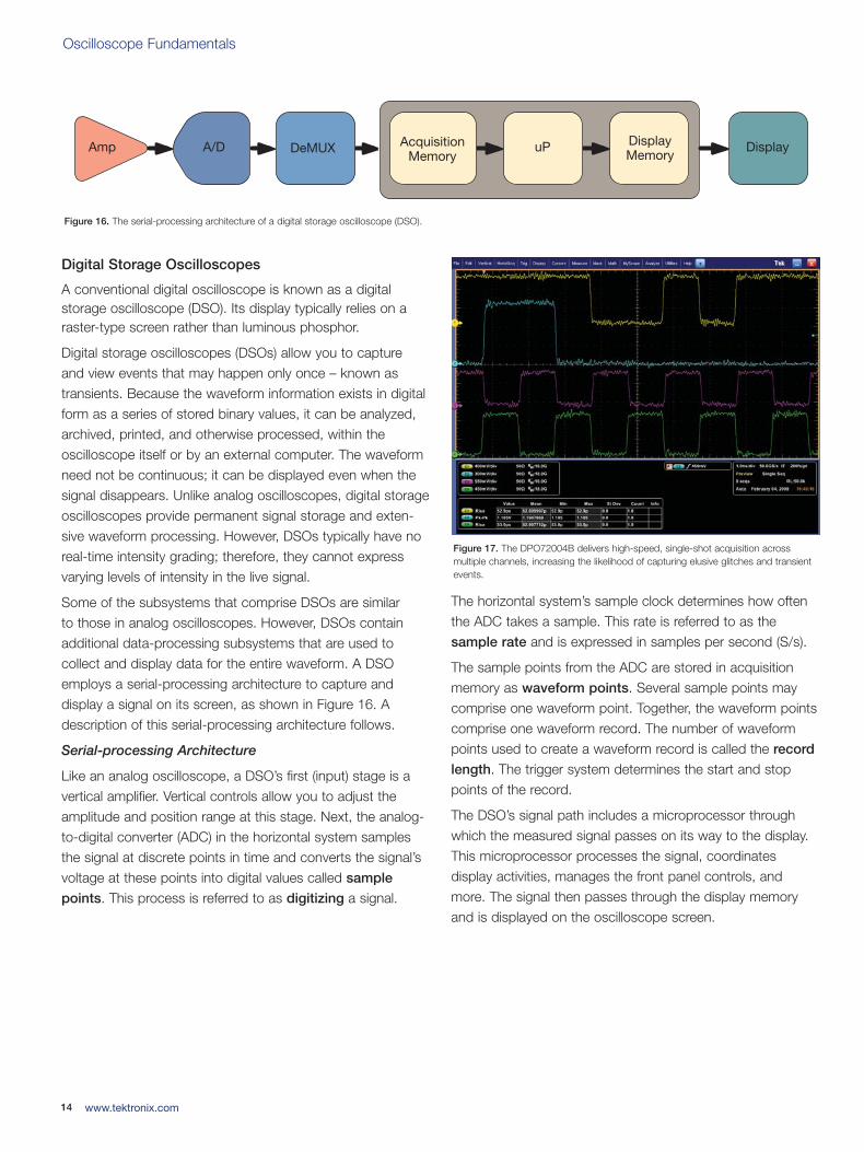
Some of the subsystems that comprise DSOs are similar to those in analog oscilloscopes. However, DSOs containadditional data-processing subsystems that are used to collect and display data for the entire waveform. A DSOemploys a serial-processing architecture to capture and display a signal on its screen, as shown in Figure 16. Adescription of this serial-processing architecture follows.
Serial-processing Architecture
Like an analog oscilloscope, a DSO’s first (input) stage is avertical amplifier. Vertical controls allow you to adjust theamplitude and position range at this stage. Next, the analog-to-digital converter (ADC) in the horizontal system samplesthe signal at discrete points in time and converts the signal’svoltage at these points into digital values called sample
points. This process is referred to as digitizing a signal.
The horizontal system’s sample clock determines how oftenthe ADC takes a sample. This rate is referred to as the sample rate and is expressed in samples per second (S/s).
The sample points from the ADC are stored in acquisitionmemory as waveform points. Several sample points maycomprise one waveform point. Together, the waveform pointscomprise one waveform record. The number of waveformpoints used to create a waveform record is called the record
length. The trigger system determines the start and stoppoints of the record.
The DSO’s signal path includes a microprocessor throughwhich the measured signal passes on its way to the display.This microprocessor processes the signal, coordinates display activities, manages the front panel controls, andmore. The signal then passes through the display memoryand is displayed on the oscilloscope screen.
14 www.tektronix.com
Amp A/D DeMUX DisplayuP DisplayMemory
AcquisitionMemory
Figure 16. The serial-processing architecture of a digital storage oscilloscope (DSO).
Figure 17. The DPO72004B delivers high-speed, single-shot acquisition across multiple channels, increasing the likelihood of capturing elusive glitches and transientevents.
03W-8605-4_edu.qxd 3/31/09 1:55 PM Page 14
Oscilloscope Fundamentals
15www.tektronix.com
Depending on the capabilities of your oscilloscope, additionalprocessing of the sample points may take place, whichenhances the display. Pre-trigger may also be available,enabling you to see events before the trigger point. Most of today’s digital oscilloscopes also provide a selection of automatic parametric measurements, simplifying themeasurement process.
A DSO provides high performance in a single-shot, multi-channel instrument (see Figure 17). DSOs are ideal for low-repetition-rate or single-shot, high-speed, multi-channel design applications. In the real world of digitaldesign, an engineer usually examines four or more signalssimultaneously, making the DSO a critical companion.
Digital Phosphor Oscilloscopes
The digital phosphor oscilloscope (DPO) offers a newapproach to oscilloscope architecture. This architectureenables a DPO to deliver unique acquisition and displaycapabilities to accurately reconstruct a signal.
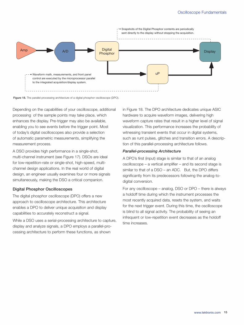
While a DSO uses a serial-processing architecture to capture,display and analyze signals, a DPO employs a parallel-pro-cessing architecture to perform these functions, as shown
in Figure 18. The DPO architecture dedicates unique ASIChardware to acquire waveform images, delivering high waveform capture rates that result in a higher level of signalvisualization. This performance increases the probability ofwitnessing transient events that occur in digital systems, such as runt pulses, glitches and transition errors. A descrip-tion of this parallel-processing architecture follows.
Parallel-processing Architecture
A DPO’s first (input) stage is similar to that of an analog oscilloscope – a vertical amplifier – and its second stage issimilar to that of a DSO – an ADC. But, the DPO differs significantly from its predecessors following the analog-to-digital conversion.
For any oscilloscope – analog, DSO or DPO – there is alwaysa holdoff time during which the instrument processes themost recently acquired data, resets the system, and waits for the next trigger event. During this time, the oscilloscope is blind to all signal activity. The probability of seeing an infrequent or low-repetition event decreases as the holdofftime increases.
• Snapshots of the Digital Phosphor contents are periodically sent directly to the display without stopping the acquisition.
• Waveform math, measurements, and front panel control are executed by the microprocessor parallel to the integrated acquisition/display system.
Amp A/D Display
uP
DigitalPhosphor
Figure 18. The parallel-processing architecture of a digital phosphor oscilloscope (DPO).
03W-8605-4_edu.qxd 3/31/09 1:55 PM Page 15
Oscilloscope Fundamentals
It should be noted that it is impossible to determine the probability of capture by simply looking at the display updaterate. If you rely solely on the update rate, it is easy to makethe mistake of believing that the oscilloscope is capturing all pertinent information about the waveform when, in fact, it is not.
The digital storage oscilloscope processes captured wave-forms serially. The speed of its microprocessor is a bottleneckin this process because it limits the waveform capture rate.
The DPO rasterizes the digitized waveform data into a digitalphosphor database. Every 1/30th of a second – about as fastas the human eye can perceive it – a snapshot of the signalimage that is stored in the database is pipelined directly tothe display system. This direct rasterization of waveform data,and direct copy to display memory from the database,removes the data-processing bottleneck inherent in otherarchitectures. The result is an enhanced “live-time” and livelydisplay update. Signal details, intermittent events, anddynamic characteristics of the signal are captured in real-time. The DPO’s microprocessor works in parallel with thisintegrated acquisition system for display management, measurement automation and instrument control, so that itdoes not affect the oscilloscope’s acquisition speed.
A DPO faithfully emulates the best display attributes of ananalog oscilloscope, displaying the signal in three dimen-sions: time, amplitude and the distribution of amplitude overtime, all in real time.
Unlike an analog oscilloscope’s reliance on chemical phos-phor, a DPO uses a purely electronic digital phosphor that’sactually a continuously updated database. This database hasa separate “cell” of information for every single pixel in theoscilloscope’s display. Each time a waveform is captured – in other words, every time the oscilloscope triggers – it ismapped into the digital phosphor database’s cells. Each cellthat represents a screen location and is touched by thewaveform is reinforced with intensity information, while othercells are not. Thus, intensity information builds up in cellswhere the waveform passes most often.
When the digital phosphor database is fed to the oscillo-scope’s display, the display reveals intensified waveformareas, in proportion to the signal’s frequency of occurrence at each point – much like the intensity grading characteristicsof an analog oscilloscope. The DPO also allows the display of the varying frequency-of-occurence information on the display as contrasting colors, unlike an analog oscilloscope.With a DPO, it is easy to see the difference between a waveform that occurs on almost every trigger and one thatoccurs, say, every 100th trigger.
Digital phosphor oscilloscopes (DPOs) break down the barrierbetween analog and digital oscilloscope technologies. Theyare equally suitable for viewing high and low frequencies,repetitive waveforms, transients, and signal variations in realtime. Only a DPO provides the Z (intensity) axis in real timethat is missing from conventional DSOs.
A DPO is ideal for those who need the best general-purposedesign and troubleshooting tool for a wide range of applica-tions (see Figure 19). A DPO is exemplary for communicationmask testing, digital debug of intermittent signals, repetitivedigital design and timing applications.
16 www.tektronix.com
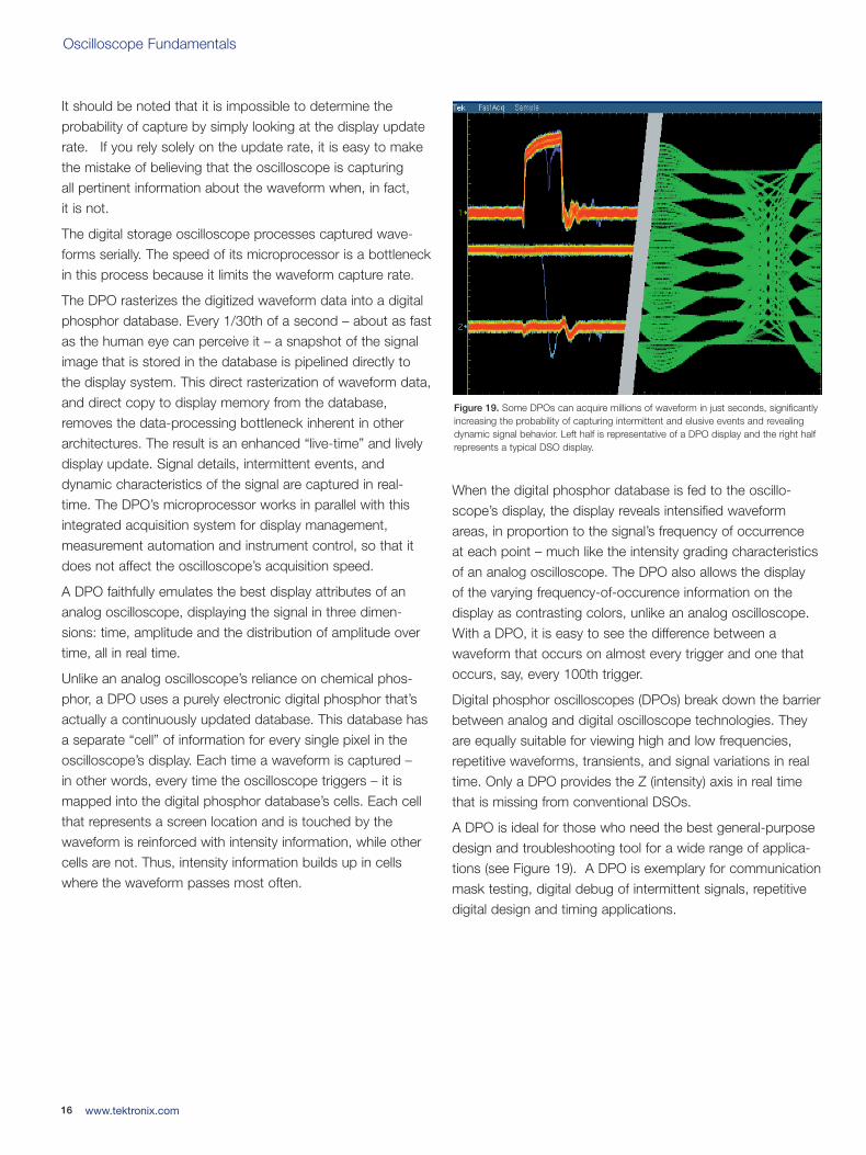
Figure 19. Some DPOs can acquire millions of waveform in just seconds, significantlyincreasing the probability of capturing intermittent and elusive events and revealingdynamic signal behavior. Left half is representative of a DPO display and the right halfrepresents a typical DSO display.
03W-8605-4_edu.qxd 3/31/09 1:55 PM Page 16
Oscilloscope Fundamentals
17www.tektronix.com
Digital Sampling Oscilloscopes
When measuring high-frequency signals, the oscilloscopemay not be able to collect enough samples in one sweep.A digital sampling oscilloscope is an ideal tool for accuratelycapturing signals whose frequency components are muchhigher than the oscilloscope’s sample rate (see Figure 21).This oscilloscope is capable of measuring signals of up to an order of magnitude faster than any other oscilloscope. It can achieve bandwidth and high-speed timing ten timeshigher than other oscilloscopes for repetitive signals.Sequential equivalent-time sampling oscilloscopes are available with bandwidths to 80 GHz.
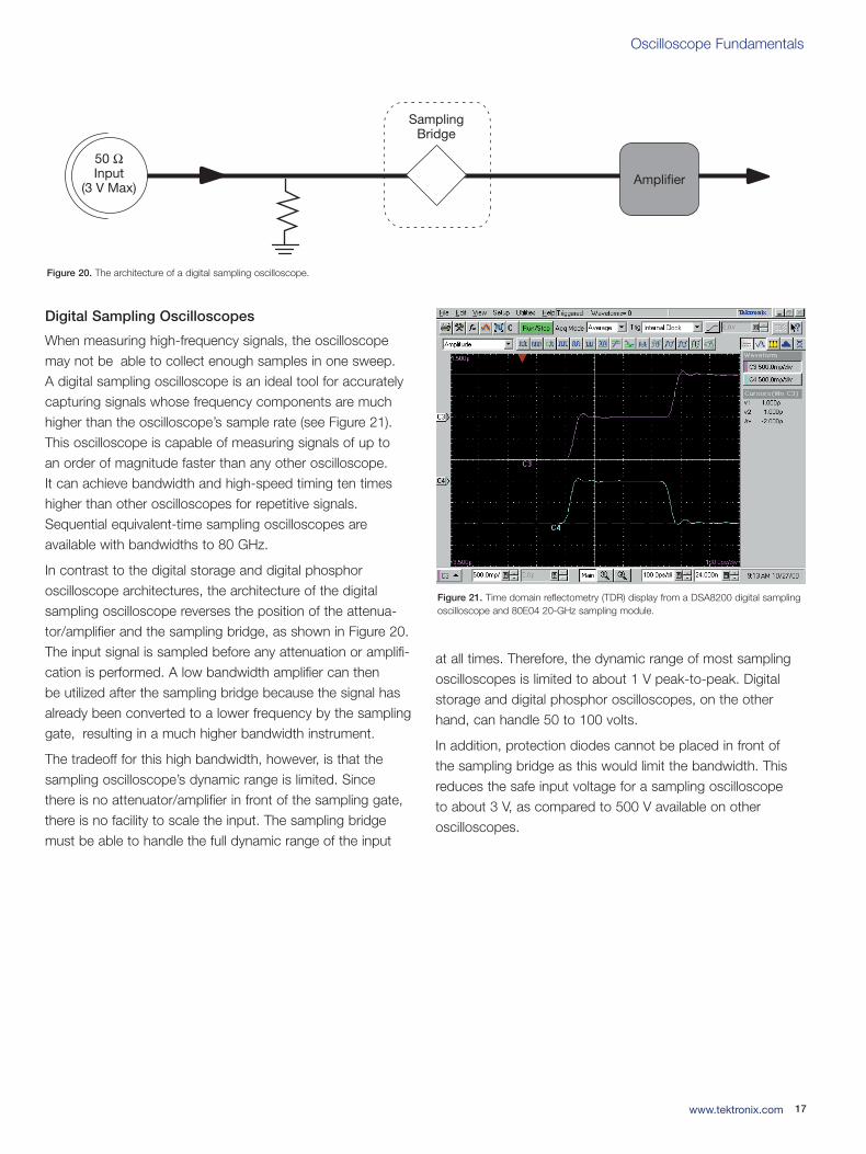
In contrast to the digital storage and digital phosphor oscilloscope architectures, the architecture of the digital sampling oscilloscope reverses the position of the attenua-tor/amplifier and the sampling bridge, as shown in Figure 20.The input signal is sampled before any attenuation or amplifi-cation is performed. A low bandwidth amplifier can then be utilized after the sampling bridge because the signal hasalready been converted to a lower frequency by the samplinggate, resulting in a much higher bandwidth instrument.
The tradeoff for this high bandwidth, however, is that thesampling oscilloscope’s dynamic range is limited. Since there is no attenuator/amplifier in front of the sampling gate,there is no facility to scale the input. The sampling bridgemust be able to handle the full dynamic range of the input
at all times. Therefore, the dynamic range of most samplingoscilloscopes is limited to about 1 V peak-to-peak. Digitalstorage and digital phosphor oscilloscopes, on the otherhand, can handle 50 to 100 volts.
In addition, protection diodes cannot be placed in front of the sampling bridge as this would limit the bandwidth. Thisreduces the safe input voltage for a sampling oscilloscope to about 3 V, as compared to 500 V available on other oscilloscopes.
SamplingBridge
Amplifier
50 ΩInput
(3 V Max)
Figure 20. The architecture of a digital sampling oscilloscope.
Figure 21. Time domain reflectometry (TDR) display from a DSA8200 digital samplingoscilloscope and 80E04 20-GHz sampling module.
03W-8605-4_edu.qxd 3/31/09 1:55 PM Page 17
Oscilloscope Fundamentals
The Systems and Controls of anOscilloscope
A basic oscilloscope consists of four differentsystems – the vertical system, horizontal system, trigger system, and display system.Understanding each of these systems will enable you to effectively apply the oscilloscopeto tackle your specific measurement challenges.Recall that each system contributes to the oscilloscope’s ability to accurately reconstruct a signal.
This section briefly describes the basic systems and controlsfound on analog and digital oscilloscopes. Some controls differ between analog and digital oscilloscopes; your oscillo-scope probably has additional controls not discussed here.
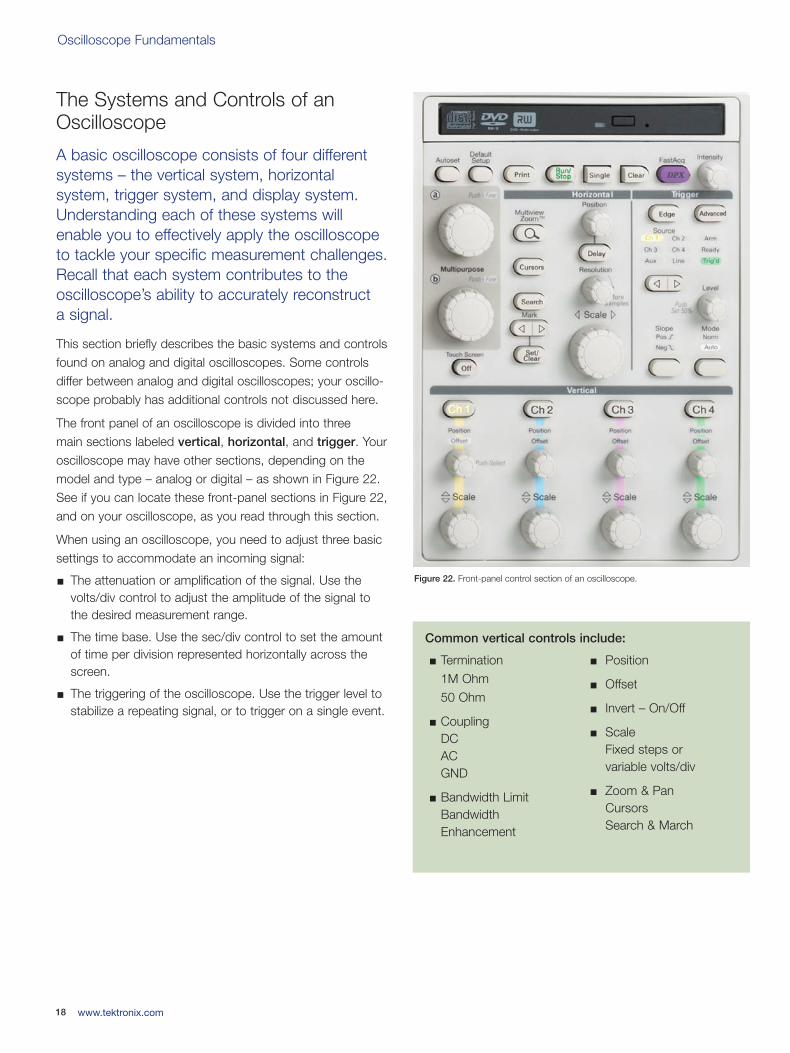
The front panel of an oscilloscope is divided into three main sections labeled vertical, horizontal, and trigger. Youroscilloscope may have other sections, depending on themodel and type – analog or digital – as shown in Figure 22.See if you can locate these front-panel sections in Figure 22,and on your oscilloscope, as you read through this section.
When using an oscilloscope, you need to adjust three basicsettings to accommodate an incoming signal:
The attenuation or amplification of the signal. Use thevolts/div control to adjust the amplitude of the signal to the desired measurement range.
The time base. Use the sec/div control to set the amountof time per division represented horizontally across thescreen.
The triggering of the oscilloscope. Use the trigger level tostabilize a repeating signal, or to trigger on a single event.
18 www.tektronix.com
Figure 22. Front-panel control section of an oscilloscope.
Termination1M Ohm50 Ohm
CouplingDCACGND
Bandwidth LimitBandwidth Enhancement
Position
Offset
Invert – On/Off
ScaleFixed steps or variable volts/div
Zoom & PanCursorsSearch & March
Common vertical controls include:
03W-8605-4_edu.qxd 3/31/09 1:55 PM Page 18
Oscilloscope Fundamentals
19www.tektronix.com
Vertical System and Controls
Vertical controls can be used to position and scale the waveform vertically. Vertical controls can also be used to setthe input coupling and other signal conditioning, describedlater in this section.
Position and Volts per Division
The vertical position control allows you to move the waveformup and down exactly where you want it on the screen.
The volts-per-division setting (usually written as volts/div)varies the size of the waveform on the screen.
The volts/div setting is a scale factor. If the volts/div setting is 5 volts, then each of the eight vertical divisions represents 5 volts and the entire screen can display 40 volts from bot-tom to top, assuming a graticule with eight major divisions. If the setting is 0.5 volts/div, the screen can display 4 voltsfrom bottom to top, and so on. The maximum voltage youcan display on the screen is the volts/div setting multipliedby the number of vertical divisions. Note that the probe youuse, 1X or 10X, also influences the scale factor. You mustdivide the volts/div scale by the attenuation factor of theprobe if the oscilloscope does not do it for you.
Often the volts/div scale has either a variable gain or a finegain control for scaling a displayed signal to a certain numberof divisions. Use this control to assist in taking rise timemeasurements.
Input Coupling
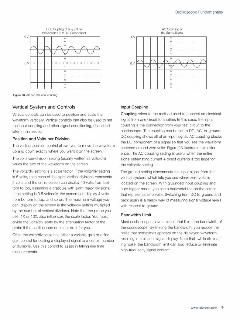
Coupling refers to the method used to connect an electricalsignal from one circuit to another. In this case, the input coupling is the connection from your test circuit to the oscilloscope. The coupling can be set to DC, AC, or ground.DC coupling shows all of an input signal. AC coupling blocksthe DC component of a signal so that you see the waveformcentered around zero volts. Figure 23 illustrates this differ-ence. The AC coupling setting is useful when the entire signal (alternating current + direct current) is too large for the volts/div setting.
The ground setting disconnects the input signal from the vertical system, which lets you see where zero volts is located on the screen. With grounded input coupling andauto trigger mode, you see a horizontal line on the screenthat represents zero volts. Switching from DC to ground andback again is a handy way of measuring signal voltage levelswith respect to ground.
Bandwidth Limit
Most oscilloscopes have a circuit that limits the bandwidth ofthe oscilloscope. By limiting the bandwidth, you reduce thenoise that sometimes appears on the displayed waveform,resulting in a cleaner signal display. Note that, while eliminat-ing noise, the bandwidth limit can also reduce or eliminatehigh-frequency signal content.
4 V
0 V
AC Coupling ofthe Same Signal
4 V
0 V
DC Coupling of a V SineWave with a 2 V DC Component
p-p
Figure 23. AC and DC input coupling.
03W-8605-4_edu.qxd 3/31/09 1:55 PM Page 19
Oscilloscope Fundamentals
Bandwidth Enhancement
Some oscilloscopes may provide a DSP arbitrary equalizationfilter which can be used to improve the oscilloscope channelresponse. This filter extends the bandwidth, flattens the oscilloscope channel frequency response, improves phaselinearity, and provides a better match between channels. It also decreases risetime and improves the time domain step response.
Horizontal System and Controls
An oscilloscope’s horizontal system is most closely associated with its acquisition of an input signal – samplerate and record length are among the considerations here.Horizontal controls are used to position and scale the waveform horizontally.
Acquisition Controls
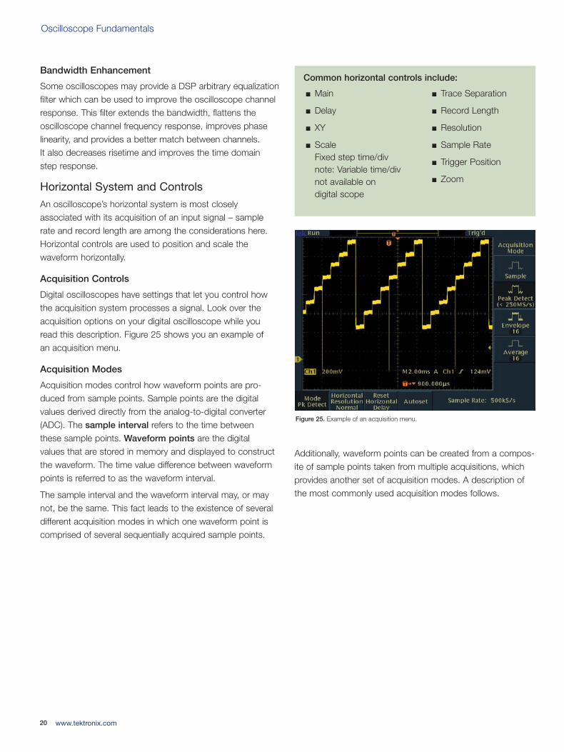
Digital oscilloscopes have settings that let you control howthe acquisition system processes a signal. Look over theacquisition options on your digital oscilloscope while you read this description. Figure 25 shows you an example of an acquisition menu.
Acquisition Modes
Acquisition modes control how waveform points are pro-duced from sample points. Sample points are the digital values derived directly from the analog-to-digital converter(ADC). The sample interval refers to the time between these sample points. Waveform points are the digital values that are stored in memory and displayed to constructthe waveform. The time value difference between waveformpoints is referred to as the waveform interval.
The sample interval and the waveform interval may, or maynot, be the same. This fact leads to the existence of severaldifferent acquisition modes in which one waveform point iscomprised of several sequentially acquired sample points.
Additionally, waveform points can be created from a compos-ite of sample points taken from multiple acquisitions, whichprovides another set of acquisition modes. A description ofthe most commonly used acquisition modes follows.
20 www.tektronix.com
Main
Delay
XY
ScaleFixed step time/divnote: Variable time/divnot available ondigital scope
Trace Separation
Record Length
Resolution
Sample Rate
Trigger Position
Zoom
Common horizontal controls include:
Figure 25. Example of an acquisition menu.
03W-8605-4_edu.qxd 3/31/09 1:55 PM Page 20
Oscilloscope Fundamentals
21www.tektronix.com
Types of Acquisition Modes
Sample Mode: This is the simplest acquisition mode. The oscilloscope creates a waveform point by saving onesample point during each waveform interval.
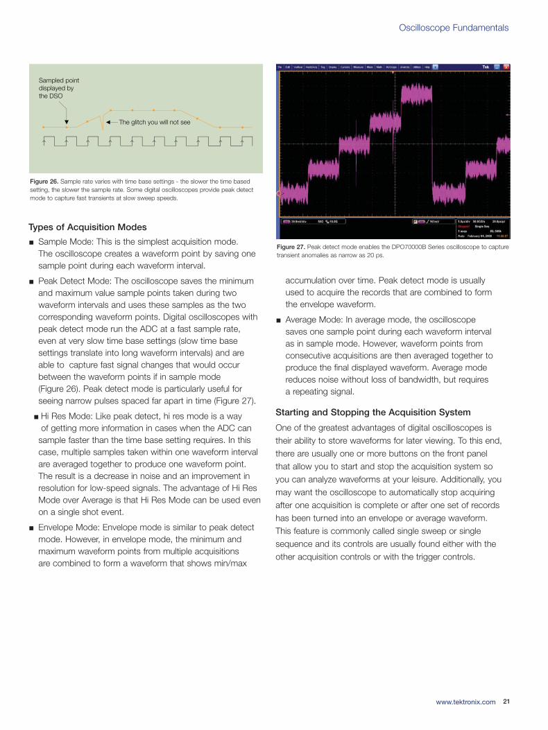
Peak Detect Mode: The oscilloscope saves the minimumand maximum value sample points taken during two waveform intervals and uses these samples as the twocorresponding waveform points. Digital oscilloscopes withpeak detect mode run the ADC at a fast sample rate, even at very slow time base settings (slow time base settings translate into long waveform intervals) and areable to capture fast signal changes that would occurbetween the waveform points if in sample mode (Figure 26). Peak detect mode is particularly useful for seeing narrow pulses spaced far apart in time (Figure 27).
Hi Res Mode: Like peak detect, hi res mode is a wayof getting more information in cases when the ADC can
sample faster than the time base setting requires. In thiscase, multiple samples taken within one waveform intervalare averaged together to produce one waveform point.The result is a decrease in noise and an improvement inresolution for low-speed signals. The advantage of Hi ResMode over Average is that Hi Res Mode can be used evenon a single shot event.
Envelope Mode: Envelope mode is similar to peak detectmode. However, in envelope mode, the minimum andmaximum waveform points from multiple acquisitions are combined to form a waveform that shows min/max
accumulation over time. Peak detect mode is usually used to acquire the records that are combined to form the envelope waveform.
Average Mode: In average mode, the oscilloscope saves one sample point during each waveform interval as in sample mode. However, waveform points from consecutive acquisitions are then averaged together toproduce the final displayed waveform. Average modereduces noise without loss of bandwidth, but requires a repeating signal.
Starting and Stopping the Acquisition System
One of the greatest advantages of digital oscilloscopes istheir ability to store waveforms for later viewing. To this end,there are usually one or more buttons on the front panel that allow you to start and stop the acquisition system so you can analyze waveforms at your leisure. Additionally, youmay want the oscilloscope to automatically stop acquiringafter one acquisition is complete or after one set of recordshas been turned into an envelope or average waveform. This feature is commonly called single sweep or singlesequence and its controls are usually found either with theother acquisition controls or with the trigger controls.
The glitch you will not see
Sampled point displayed by the DSO
Figure 26. Sample rate varies with time base settings - the slower the time basedsetting, the slower the sample rate. Some digital oscilloscopes provide peak detectmode to capture fast transients at slow sweep speeds.
Figure 27. Peak detect mode enables the DPO70000B Series oscilloscope to capturetransient anomalies as narrow as 20 ps.
03W-8605-4_edu.qxd 3/31/09 1:55 PM Page 21
Oscilloscope Fundamentals
Sampling
Sampling is the process of converting a portion of an input signal into a number of discrete electrical values for the purpose of storage, processing and/or display. The magnitude of each sampled point is equal to the amplitude of the input signal at the instant in time in which the signal is sampled.
Sampling is like taking snapshots. Each snapshot corre-sponds to a specific point in time on the waveform. Thesesnapshots can then be arranged in the appropriate order intime so as to reconstruct the input signal.
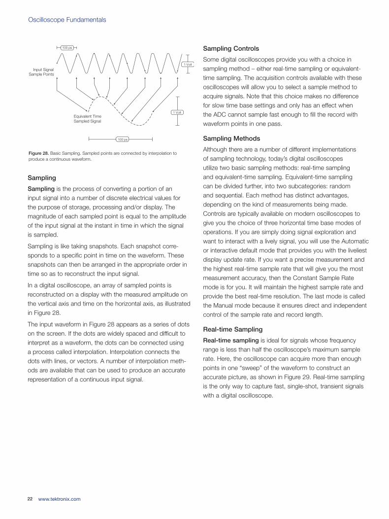
In a digital oscilloscope, an array of sampled points is reconstructed on a display with the measured amplitude onthe vertical axis and time on the horizontal axis, as illustratedin Figure 28.
The input waveform in Figure 28 appears as a series of dotson the screen. If the dots are widely spaced and difficult tointerpret as a waveform, the dots can be connected using a process called interpolation. Interpolation connects the dots with lines, or vectors. A number of interpolation meth-ods are available that can be used to produce an accuraterepresentation of a continuous input signal.
Sampling Controls
Some digital oscilloscopes provide you with a choice in sampling method – either real-time sampling or equivalent-time sampling. The acquisition controls available with theseoscilloscopes will allow you to select a sample method toacquire signals. Note that this choice makes no difference for slow time base settings and only has an effect when the ADC cannot sample fast enough to fill the record withwaveform points in one pass.
Sampling Methods
Although there are a number of different implementations of sampling technology, today’s digital oscilloscopes utilize two basic sampling methods: real-time sampling and equivalent-time sampling. Equivalent-time sampling can be divided further, into two subcategories: random and sequential. Each method has distinct advantages, depending on the kind of measurements being made.Controls are typically available on modern oscilloscopes togive you the choice of three horizontal time base modes ofoperations. If you are simply doing signal exploration andwant to interact with a lively signal, you will use the Automaticor interactive default mode that provides you with the liveliestdisplay update rate. If you want a precise measurement andthe highest real-time sample rate that will give you the mostmeasurement accuracy, then the Constant Sample Ratemode is for you. It will maintain the highest sample rate andprovide the best real-time resolution. The last mode is calledthe Manual mode because it ensures direct and independentcontrol of the sample rate and record length.
Real-time Sampling
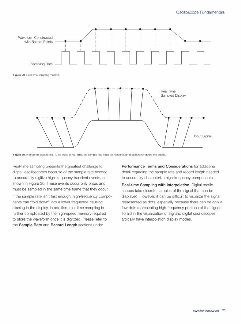
Real-time sampling is ideal for signals whose frequencyrange is less than half the oscilloscope’s maximum samplerate. Here, the oscilloscope can acquire more than enoughpoints in one “sweep” of the waveform to construct an accurate picture, as shown in Figure 29. Real-time samplingis the only way to capture fast, single-shot, transient signalswith a digital oscilloscope.
22 www.tektronix.com
Input SignalSample Points
100 ps
1 Volt
100 ps
1 Volt
Equivalent TimeSampled Signal
Figure 28. Basic Sampling. Sampled points are connected by interpolation to produce a continuous waveform.
03W-8605-4_edu.qxd 3/31/09 1:55 PM Page 22
Oscilloscope Fundamentals
23www.tektronix.com
Real-time sampling presents the greatest challenge for digital oscilloscopes because of the sample rate needed to accurately digitize high-frequency transient events, asshown in Figure 30. These events occur only once, and must be sampled in the same time frame that they occur.
If the sample rate isn’t fast enough, high-frequency compo-nents can “fold down” into a lower frequency, causing aliasing in the display. In addition, real-time sampling is further complicated by the high-speed memory required to store the waveform once it is digitized. Please refer to the Sample Rate and Record Length sections under
Performance Terms and Considerations for additionaldetail regarding the sample rate and record length needed to accurately characterize high-frequency components.
Real-time Sampling with Interpolation. Digital oscillo-scopes take discrete samples of the signal that can be displayed. However, it can be difficult to visualize the signalrepresented as dots, especially because there can be only afew dots representing high-frequency portions of the signal.To aid in the visualization of signals, digital oscilloscopes typically have interpolation display modes.
Sampling Rate
Waveform Constructedwith Record Points
Figure 29. Real-time sampling method.
Real TimeSampled Display
Input Signal
Figure 30. In order to capture this 10 ns pulse in real-time, the sample rate must be high enough to accurately define the edges.
03W-8605-4_edu.qxd 3/31/09 1:55 PM Page 23
Oscilloscope Fundamentals
In simple terms, interpolation “connects the dots” so that a signal that is sampled only a few times in each cycle can be accurately displayed. Using real-time sampling with interpolation, the oscilloscope collects a few sample points of the signal in a single pass in real-time mode and usesinterpolation to fill in the gaps. Interpolation is a processingtechnique used to estimate what the waveform looks likebased on a few points.
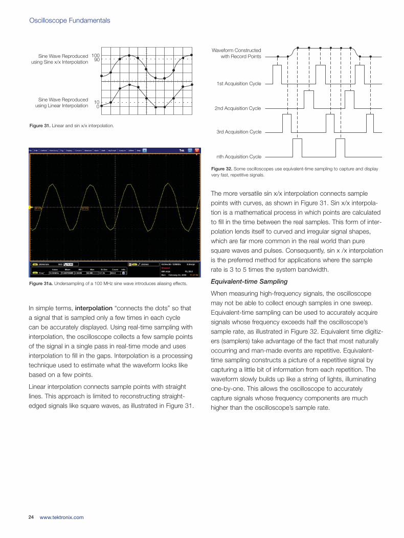
Linear interpolation connects sample points with straightlines. This approach is limited to reconstructing straight-edged signals like square waves, as illustrated in Figure 31.
The more versatile sin x/x interpolation connects samplepoints with curves, as shown in Figure 31. Sin x/x interpola-tion is a mathematical process in which points are calculatedto fill in the time between the real samples. This form of inter-polation lends itself to curved and irregular signal shapes,which are far more common in the real world than puresquare waves and pulses. Consequently, sin x /x interpolationis the preferred method for applications where the samplerate is 3 to 5 times the system bandwidth.
Equivalent-time Sampling
When measuring high-frequency signals, the oscilloscopemay not be able to collect enough samples in one sweep.Equivalent-time sampling can be used to accurately acquiresignals whose frequency exceeds half the oscilloscope’ssample rate, as illustrated in Figure 32. Equivalent time digitiz-ers (samplers) take advantage of the fact that most naturallyoccurring and man-made events are repetitive. Equivalent-time sampling constructs a picture of a repetitive signal bycapturing a little bit of information from each repetition. Thewaveform slowly builds up like a string of lights, illuminatingone-by-one. This allows the oscilloscope to accurately capture signals whose frequency components are muchhigher than the oscilloscope’s sample rate.
24 www.tektronix.com
10090
100
Sine Wave Reproducedusing Sine x/x Interpolation
Sine Wave Reproducedusing Linear Interpolation
Figure 31. Linear and sin x/x interpolation.
1st Acquisition Cycle
2nd Acquisition Cycle
3rd Acquisition Cycle
nth Acquisition Cycle
Waveform Constructedwith Record Points
Figure 32. Some oscilloscopes use equivalent-time sampling to capture and displayvery fast, repetitive signals.
Figure 31a. Undersampling of a 100 MHz sine wave introduces aliasing effects.
03W-8605-4_edu.qxd 3/31/09 1:55 PM Page 24
Oscilloscope Fundamentals
25www.tektronix.com
There are two types of equivalent-time sampling methods:random and sequential. Each has its advantages. Random
equivalent-time sampling allows display of the input signalprior to the trigger point, without the use of a delay line.Sequential equivalent-time sampling provides muchgreater time resolution and accuracy. Both require that theinput signal be repetitive.
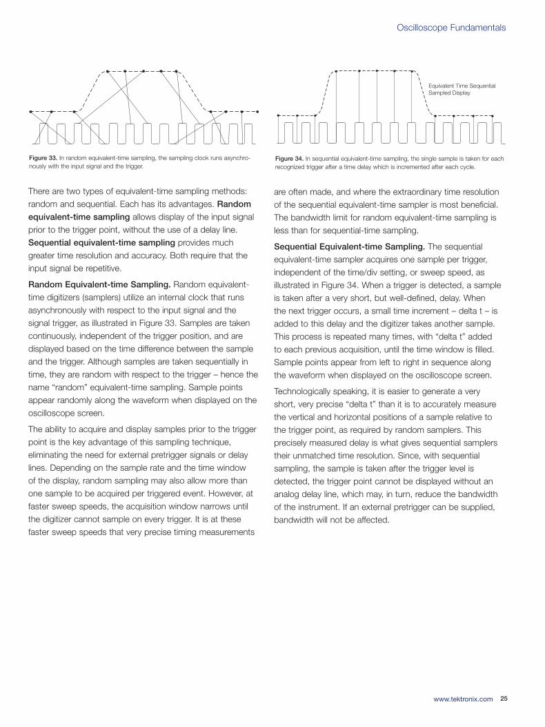
Random Equivalent-time Sampling. Random equivalent-time digitizers (samplers) utilize an internal clock that runsasynchronously with respect to the input signal and the signal trigger, as illustrated in Figure 33. Samples are takencontinuously, independent of the trigger position, and are displayed based on the time difference between the sampleand the trigger. Although samples are taken sequentially intime, they are random with respect to the trigger – hence thename “random” equivalent-time sampling. Sample pointsappear randomly along the waveform when displayed on theoscilloscope screen.
The ability to acquire and display samples prior to the triggerpoint is the key advantage of this sampling technique, eliminating the need for external pretrigger signals or delaylines. Depending on the sample rate and the time window of the display, random sampling may also allow more thanone sample to be acquired per triggered event. However, atfaster sweep speeds, the acquisition window narrows untilthe digitizer cannot sample on every trigger. It is at thesefaster sweep speeds that very precise timing measurements
are often made, and where the extraordinary time resolutionof the sequential equivalent-time sampler is most beneficial.The bandwidth limit for random equivalent-time sampling isless than for sequential-time sampling.
Sequential Equivalent-time Sampling. The sequentialequivalent-time sampler acquires one sample per trigger,independent of the time/div setting, or sweep speed, as illustrated in Figure 34. When a trigger is detected, a sampleis taken after a very short, but well-defined, delay. When the next trigger occurs, a small time increment – delta t – isadded to this delay and the digitizer takes another sample.This process is repeated many times, with “delta t” added to each previous acquisition, until the time window is filled.Sample points appear from left to right in sequence along the waveform when displayed on the oscilloscope screen.
Technologically speaking, it is easier to generate a very short, very precise “delta t” than it is to accurately measurethe vertical and horizontal positions of a sample relative to the trigger point, as required by random samplers. This precisely measured delay is what gives sequential samplerstheir unmatched time resolution. Since, with sequential sampling, the sample is taken after the trigger level is detected, the trigger point cannot be displayed without ananalog delay line, which may, in turn, reduce the bandwidthof the instrument. If an external pretrigger can be supplied,bandwidth will not be affected.
Figure 33. In random equivalent-time sampling, the sampling clock runs asynchro-nously with the input signal and the trigger.
Equivalent Time SequentialSampled Display
Figure 34. In sequential equivalent-time sampling, the single sample is taken for eachrecognized trigger after a time delay which is incremented after each cycle.
03W-8605-4_edu.qxd 3/31/09 1:55 PM Page 25
Oscilloscope Fundamentals
Position and Seconds per Division
The horizontal position control moves the waveform left andright to exactly where you want it on the screen.
The seconds-per-division setting (usually written as sec/div)lets you select the rate at which the waveform is drawnacross the screen (also known as the time base setting orsweep speed). This setting is a scale factor. If the setting is 1 ms, each horizontal division represents 1 ms and the totalscreen width represents 10 ms, or ten divisions. Changingthe sec/div setting enables you to look at longer and shortertime intervals of the input signal.
As with the vertical volts/div scale, the horizontal sec/divscale may have variable timing, allowing you to set the horizontal time scale between the discrete settings.
Time Base Selections
Your oscilloscope has a time base, which is usually referredto as the main time base. Many oscilloscopes also have whatis called a delayed time base – a time base with a sweepthat can start (or be triggered to start) relative to a pre-deter-mined time on the main time base sweep. Using a delayedtime base sweep allows you to see events more clearly andto see events that are not visible solely with the main timebase sweep.
The delayed time base requires the setting of a time delayand the possible use of delayed trigger modes and other settings not described in this primer. Refer to the manualsupplied with your oscilloscope for information on how to use these features.
Zoom
Your oscilloscope may have special horizontal magnificationsettings that let you display a magnified section of the waveform on-screen. Some oscilloscopes add pan functionsto the zoom capability. Knobs are used to adjust zoom factoror scale and the pan of the zoom box across the waveform.The operation in a digital storage oscilloscope (DSO) is performed on stored digitized data.
XY Mode
Most oscilloscopes have an XY mode that lets you display an input signal, rather than the time base, on the horizontalaxis. This mode of operation opens up a whole new area of phase shift measurement techniques, explained in theMeasurement Techniques section of this primer.
Z Axis
A digital phosphor oscilloscope (DPO) has a high displaysample density and an innate ability to capture intensity information. With its intensity axis (Z axis), the DPO is able to provide a three-dimensional, real-time display similar tothat of an analog oscilloscope. As you look at the waveformtrace on a DPO, you can see brightened areas – the areaswhere a signal occurs most often. This display makes it easyto distinguish the basic signal shape from a transient thatoccurs only once in a while – the basic signal would appearmuch brighter. One application of the Z axis is to feed specialtimed signals into the separate Z input to create highlighted“marker” dots at known intervals in the waveform.
XYZ Mode with DPO and XYZ Record Display
Some DPOs can use the Z input to create an XY display with intensity grading. In this case, the DPO samples theinstantaneous data value at the Z input and uses that valueto qualify a specific part of the waveform. Once you havequalified samples, these samples can accumulate, resulting in an intensity-graded XYZ display. XYZ mode is especiallyuseful for displaying the polar patterns commonly used intesting wireless communication devices – a constellation diagram, for example. Another method of displaying XYZ data is XYZ record display. This mode the data from theacquisition memory is used rather than the DPO database.
26 www.tektronix.com
03W-8605-4_edu.qxd 3/31/09 1:55 PM Page 26
Oscilloscope Fundamentals
27www.tektronix.com
Trigger System and Controls
An oscilloscope’s trigger function synchronizes the horizontalsweep at the correct point of the signal, essential for clearsignal characterization. Trigger controls allow you to stabilizerepetitive waveforms and capture single-shot waveforms.
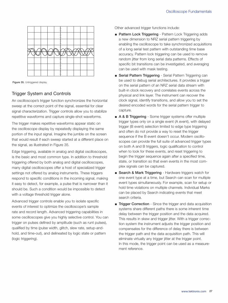
The trigger makes repetitive waveforms appear static on the oscilloscope display by repeatedly displaying the sameportion of the input signal. Imagine the jumble on the screenthat would result if each sweep started at a different place onthe signal, as illustrated in Figure 35.
Edge triggering, available in analog and digital oscilloscopes,is the basic and most common type. In addition to thresholdtriggering offered by both analog and digital oscilloscopes,many digital oscilloscopes offer a host of specialized triggersettings not offered by analog instruments. These triggersrespond to specific conditions in the incoming signal, makingit easy to detect, for example, a pulse that is narrower than itshould be. Such a condition would be impossible to detectwith a voltage threshold trigger alone.
Advanced trigger controls enable you to isolate specificevents of interest to optimize the oscilloscope’s sample rate and record length. Advanced triggering capabilities insome oscilloscopes give you highly selective control. You cantrigger on pulses defined by amplitude (such as runt pulses),qualified by time (pulse width, glitch, slew rate, setup-and-hold, and time-out), and delineated by logic state or pattern(logic triggering).
Other advanced trigger functions include:
Pattern Lock Triggering - Pattern Lock Triggering adds a new dimension to NRZ serial pattern triggering byenabling the oscilloscope to take synchronized acquisitionsof a long serial test pattern with outstanding time base accuracy. Pattern lock triggering can be used to removerandom jitter from long serial data patterns. Effects of specific bit transitions can be investigated, and averagingcan be used with mask testing.
Serial Pattern Triggering - Serial Pattern Triggering canbe used to debug serial architectures. It provides a triggeron the serial pattern of an NRZ serial data stream withbuilt-in clock recovery and correlates events across thephysical and link layer. The instrument can recover theclock signal, identify transitions, and allow you to set thedesired encoded words for the serial pattern trigger tocapture.
A & B Triggering - Some trigger systems offer multipletrigger types only on a single event (A event), with delayedtrigger (B event) selection limited to edge type triggeringand often do not provide a way to reset the triggersequence if the B event doesn’t occur. Modern oscillo-scopes can provide the full suite of advanced trigger typeson both A and B triggers, logic qualification to controlwhen to look for these events, and reset triggering tobegin the trigger sequence again after a specified time,state, or transition so that even events in the most com-plex signals can be captured.
Search & Mark Triggering - Hardware triggers watch forone event type at a time, but Search can scan for multipleevent types simultaneously. For example, scan for setup orhold time violations on multiple channels. Individual Markscan be placed by Search indicating events that meetsearch criteria.
Trigger Correction - Since the trigger and data acquisitionsystems share different paths there is some inherent timedelay between the trigger position and the data acquired.This results in skew and trigger jitter. With a trigger correc-tion system the instrument adjusts the trigger position andcompensates for the difference of delay there is betweenthe trigger path and the data acquisition path. This willeliminate virtually any trigger jitter at the trigger point. In this mode, the trigger point can be used as a measure-ment reference.
Figure 35. Untriggered display.
03W-8605-4_edu.qxd 3/31/09 1:55 PM Page 27
Serial Triggering on Specific Standard Signals I2C,CAN, LIN, etc.) - Some oscilloscopes provide the ability to trigger on specific signal types for standard serial datasignals such as CAN, LIN, I2C, SPI, and others. Thedecode of these signal types is also available on manyoscilloscopes today.
Optional trigger controls in some oscilloscopes are designedspecifically to examine communications signals. The intuitiveuser interface available in some oscilloscopes also allowsrapid setup of trigger parameters with wide flexibility in thetest setup to maximize your productivity.
When you are using more than four channels to trigger onsignals, a logic analyzer is the ideal tool. Please refer toTektronix’ XYZs of Logic Analyzers primer for more informa-tion about these valuable test and measurement instruments.
Trigger Position
Horizontal trigger position control is only available on digitaloscilloscopes. The trigger position control may be located in the horizontal control section of your oscilloscope. It actually represents the horizontal position of the trigger in the waveform record.
Varying the horizontal trigger position allows you to capturewhat a signal did before a trigger event, known as pre-trig-
ger viewing. Thus, it determines the length of viewable signalboth preceding and following a trigger point.
Digital oscilloscopes can provide pre-trigger viewing becausethey constantly process the input signal, whether or not atrigger has been received. A steady stream of data flowsthrough the oscilloscope; the trigger merely tells the oscillo-scope to save the present data in memory.In contrast, analog oscilloscopes only display the signal – that is, write it on the CRT – after receiving the trigger. Thus,pre-trigger viewing is not available in analog oscilloscopes,with the exception of a small amount of pre-trigger providedby a delay line in the vertical system.
Pre-trigger viewing is a valuable troubleshooting aid. If aproblem occurs intermittently, you can trigger on the problem,record the events that led up to it and, possibly, find thecause.
Trigger Level and Slope
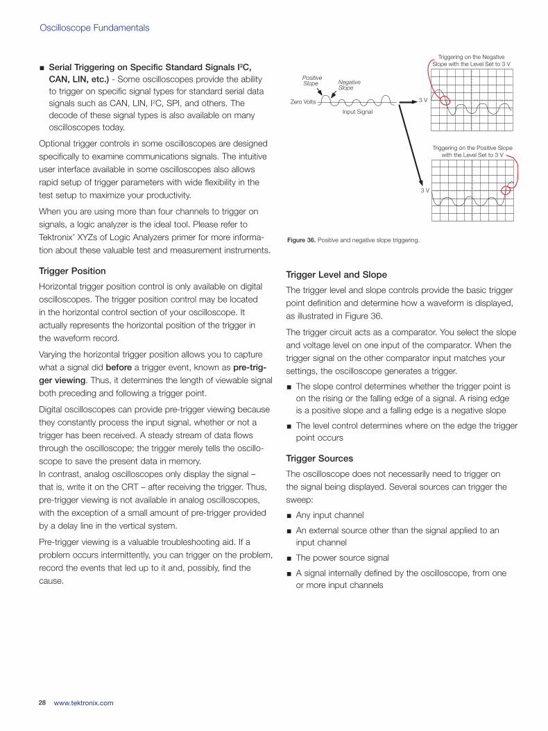
The trigger level and slope controls provide the basic triggerpoint definition and determine how a waveform is displayed,as illustrated in Figure 36.
The trigger circuit acts as a comparator. You select the slopeand voltage level on one input of the comparator. When thetrigger signal on the other comparator input matches yoursettings, the oscilloscope generates a trigger.
The slope control determines whether the trigger point ison the rising or the falling edge of a signal. A rising edge is a positive slope and a falling edge is a negative slope
The level control determines where on the edge the triggerpoint occurs
Trigger Sources
The oscilloscope does not necessarily need to trigger on the signal being displayed. Several sources can trigger thesweep:
Any input channel
An external source other than the signal applied to aninput channel
The power source signal
A signal internally defined by the oscilloscope, from one or more input channels
Oscilloscope Fundamentals
28 www.tektronix.com
3 V
3 V
PositiveSlope Negative
Slope
Input Signal
Triggering on the NegativeSlope with the Level Set to 3 V
Zero Volts
Triggering on the Positive Slopewith the Level Set to 3 V
Figure 36. Positive and negative slope triggering.
03W-8605-4_edu.qxd 3/31/09 1:55 PM Page 28
Oscilloscope Fundamentals
29www.tektronix.com
Most of the time, you can leave the oscilloscope set to trigger on the channel displayed. Some oscilloscopes providea trigger output that delivers the trigger signal to anotherinstrument.
The oscilloscope can use an alternate trigger source, whether or not it is displayed, so you should be careful not tounwittingly trigger on channel 1 while displaying channel 2,for example.
Trigger Modes
The trigger mode determines whether or not the oscillo-scope draws a waveform based on a signal condition.Common trigger modes include normal and auto.
In normal mode the oscilloscope only sweeps if the input signal reaches the set trigger point; otherwise (on an analogoscilloscope) the screen is blank or (on a digital oscilloscope)frozen on the last acquired waveform. Normal mode can bedisorienting since you may not see the signal at first if thelevel control is not adjusted correctly.
Auto mode causes the oscilloscope to sweep, even without a trigger. If no signal is present, a timer in the oscilloscopetriggers the sweep. This ensures that the display will not disappear if the signal does not cause a trigger.
In practice, you will probably use both modes: normal modebecause it lets you see just the signal of interest, even whentriggers occur at a slow rate, and auto mode because itrequires less adjustment.
Slew Rate Triggering. High frequency signalswith slew rates faster than expected or neededcan radiate troublesome energy. Slew rate trig-gering surpasses conventional edge triggeringby adding the element of time and allowing youto selectively trigger on fast or slow edges.
Glitch Triggering. Glitch triggering allows you to trigger on digital pulses when they are shorteror longer than a user-defined time limit. This trigger control enables you to examine the causes of even rare glitches and their effects on other signals
Pulse Width Triggering. Using pulse width triggering, you can monitor a signal indefinitelyand trigger on the first occurrence of a pulsewhose duration (pulse width) is outside theallowable limits.
Time-out Triggering. Time-out triggering letsyou trigger on an event without waiting for thetrigger pulse to end, by triggering based on aspecified time lapse.
Runt Pulse Triggering. Runt triggering allowsyou to capture and examine pulses that crossone logic threshold, but not both.
Trigger When:
Time:
Logic Triggering. Logic triggering allows you totrigger on any logical combination of availableinput channels – especially useful in verifying theoperation of digital logic.
Setup-and-Hold Triggering. Only setup-and-hold triggering lets you deterministically trap a single violation of setup-and-hold time thatwould almost certainly be missed by using othertrigger modes. This trigger mode makes it easyto capture specific signal quality and timingdetails when a synchronous data signal fails to meet setup-and-hold specifications.
Communication Triggering. Optionally availableon certain oscilloscope models, these triggermodes address the need to acquire a wide variety of Alternate-Mark Inversion (AMI), Code-Mark Inversion (CMI), and Non-Return to Zero (NRZ) communication signals.
03W-8605-4_edu.qxd 3/31/09 1:55 PM Page 29
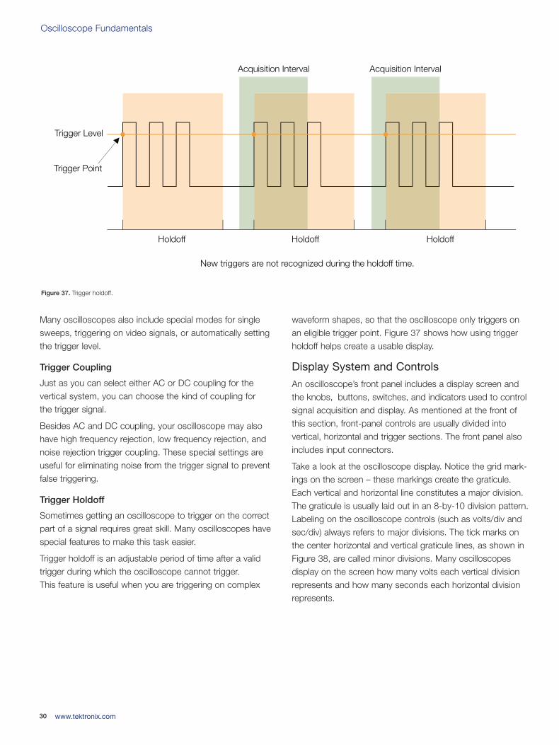
Oscilloscope Fundamentals
Many oscilloscopes also include special modes for singlesweeps, triggering on video signals, or automatically settingthe trigger level.
Trigger Coupling
Just as you can select either AC or DC coupling for the vertical system, you can choose the kind of coupling for the trigger signal.
Besides AC and DC coupling, your oscilloscope may alsohave high frequency rejection, low frequency rejection, andnoise rejection trigger coupling. These special settings areuseful for eliminating noise from the trigger signal to preventfalse triggering.
Trigger Holdoff
Sometimes getting an oscilloscope to trigger on the correctpart of a signal requires great skill. Many oscilloscopes havespecial features to make this task easier.
Trigger holdoff is an adjustable period of time after a validtrigger during which the oscilloscope cannot trigger. This feature is useful when you are triggering on complex
waveform shapes, so that the oscilloscope only triggers onan eligible trigger point. Figure 37 shows how using triggerholdoff helps create a usable display.
Display System and Controls
An oscilloscope’s front panel includes a display screen andthe knobs, buttons, switches, and indicators used to controlsignal acquisition and display. As mentioned at the front ofthis section, front-panel controls are usually divided into vertical, horizontal and trigger sections. The front panel alsoincludes input connectors.
Take a look at the oscilloscope display. Notice the grid mark-ings on the screen – these markings create the graticule.Each vertical and horizontal line constitutes a major division.The graticule is usually laid out in an 8-by-10 division pattern.Labeling on the oscilloscope controls (such as volts/div andsec/div) always refers to major divisions. The tick marks onthe center horizontal and vertical graticule lines, as shown in Figure 38, are called minor divisions. Many oscilloscopes display on the screen how many volts each vertical divisionrepresents and how many seconds each horizontal divisionrepresents.
30 www.tektronix.com
Trigger Point
Trigger Level
Acquisition Interval
New triggers are not recognized during the holdoff time.
Holdoff Holdoff Holdoff
Acquisition Interval
Figure 37. Trigger holdoff.
03W-8605-4_edu.qxd 3/31/09 1:55 PM Page 30
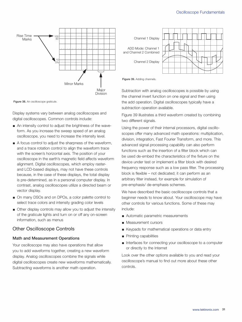
Oscilloscope Fundamentals
31www.tektronix.com
Display systems vary between analog oscilloscopes and digital oscilloscopes. Common controls include:
An intensity control to adjust the brightness of the wave-form. As you increase the sweep speed of an analog oscilloscope, you need to increase the intensity level.
A focus control to adjust the sharpness of the waveform,and a trace rotation control to align the waveform tracewith the screen’s horizontal axis. The position of your oscilloscope in the earth’s magnetic field affects waveformalignment. Digital oscilloscopes, which employ raster- and LCD-based displays, may not have these controlsbecause, in the case of these displays, the total display is pre-determined, as in a personal computer display. Incontrast, analog oscilloscopes utilize a directed beam orvector display.
On many DSOs and on DPOs, a color palette control toselect trace colors and intensity grading color levels
Other display controls may allow you to adjust the intensityof the graticule lights and turn on or off any on-screeninformation, such as menus
Other Oscilloscope Controls
Math and Measurement Operations
Your oscilloscope may also have operations that allow you to add waveforms together, creating a new waveformdisplay. Analog oscilloscopes combine the signals while digital oscilloscopes create new waveforms mathematically.Subtracting waveforms is another math operation.
Subtraction with analog oscilloscopes is possible by usingthe channel invert function on one signal and then using the add operation. Digital oscilloscopes typically have a subtraction operation available.
Figure 39 illustrates a third waveform created by combiningtwo different signals.
Using the power of their internal processors, digital oscillo-scopes offer many advanced math operations: multiplication,division, integration, Fast Fourier Transform, and more. Thisadvanced signal processing capability can also perform functions such as the insertion of a filter block which can be used de-embed the characteristics of the fixture on thedevice under test or implement a filter block with desired frequency response such as a low pass filter. The processingblock is flexible – not dedicated; it can perform as an arbitrary filter instead, for example for simulation of pre-emphasis/ de-emphasis schemes.
We have described the basic oscilloscope controls that abeginner needs to know about. Your oscilloscope may haveother controls for various functions. Some of these mayinclude:
Automatic parametric measurements
Measurement cursors
Keypads for mathematical operations or data entry
Printing capabilities
Interfaces for connecting your oscilloscope to a computeror directly to the Internet
Look over the other options available to you and read youroscilloscope’s manual to find out more about these othercontrols.
10090
100%
Minor Marks
MajorDivision
Rise TimeMarks
Figure 38. An oscilloscope graticule.
Channel 1 Display
Channel 2 Display
ADD Mode: Channel 1and Channel 2 Combined
Figure 39. Adding channels.
03W-8605-4_edu.qxd 3/31/09 1:55 PM Page 31
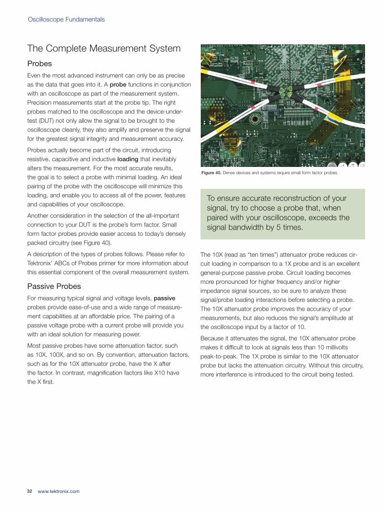
Oscilloscope Fundamentals
The Complete Measurement System
Probes
Even the most advanced instrument can only be as preciseas the data that goes into it. A probe functions in conjunctionwith an oscilloscope as part of the measurement system.Precision measurements start at the probe tip. The rightprobes matched to the oscilloscope and the device-under-test (DUT) not only allow the signal to be brought to the oscilloscope cleanly, they also amplify and preserve the signalfor the greatest signal integrity and measurement accuracy.
Probes actually become part of the circuit, introducing resistive, capacitive and inductive loading that inevitablyalters the measurement. For the most accurate results, the goal is to select a probe with minimal loading. An ideal pairing of the probe with the oscilloscope will minimize thisloading, and enable you to access all of the power, featuresand capabilities of your oscilloscope.
Another consideration in the selection of the all-importantconnection to your DUT is the probe’s form factor. Small form factor probes provide easier access to today’s denselypacked circuitry (see Figure 40).
A description of the types of probes follows. Please refer toTektronix’ ABCs of Probes primer for more information aboutthis essential component of the overall measurement system.
Passive Probes
For measuring typical signal and voltage levels, passive
probes provide ease-of-use and a wide range of measure-ment capabilities at an affordable price. The pairing of a passive voltage probe with a current probe will provide youwith an ideal solution for measuring power.
Most passive probes have some attenuation factor, such as 10X, 100X, and so on. By convention, attenuation factors,such as for the 10X attenuator probe, have the X after the factor. In contrast, magnification factors like X10 have the X first.
The 10X (read as “ten times”) attenuator probe reduces cir-cuit loading in comparison to a 1X probe and is an excellentgeneral-purpose passive probe. Circuit loading becomesmore pronounced for higher frequency and/or higher impedance signal sources, so be sure to analyze these signal/probe loading interactions before selecting a probe.The 10X attenuator probe improves the accuracy of yourmeasurements, but also reduces the signal’s amplitude at the oscilloscope input by a factor of 10.
Because it attenuates the signal, the 10X attenuator probemakes it difficult to look at signals less than 10 millivoltspeak-to-peak. The 1X probe is similar to the 10X attenuatorprobe but lacks the attenuation circuitry. Without this circuitry,more interference is introduced to the circuit being tested.
32 www.tektronix.com
Figure 40. Dense devices and systems require small form factor probes.
To ensure accurate reconstruction of yoursignal, try to choose a probe that, whenpaired with your oscilloscope, exceeds thesignal bandwidth by 5 times.
03W-8605-4_edu.qxd 3/31/09 1:55 PM Page 32
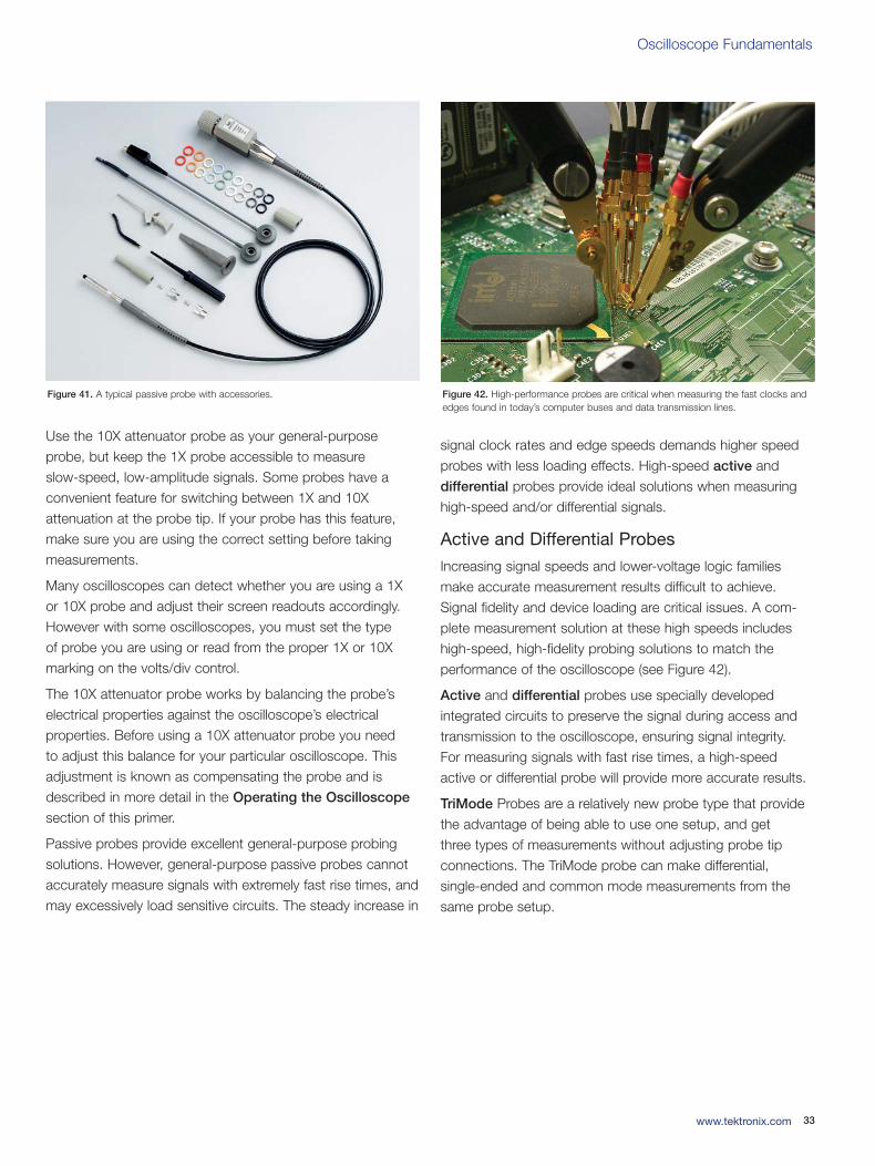
Oscilloscope Fundamentals
33www.tektronix.com
Use the 10X attenuator probe as your general-purposeprobe, but keep the 1X probe accessible to measure slow-speed, low-amplitude signals. Some probes have aconvenient feature for switching between 1X and 10X attenuation at the probe tip. If your probe has this feature,make sure you are using the correct setting before takingmeasurements.
Many oscilloscopes can detect whether you are using a 1X or 10X probe and adjust their screen readouts accordingly.However with some oscilloscopes, you must set the type of probe you are using or read from the proper 1X or 10Xmarking on the volts/div control.
The 10X attenuator probe works by balancing the probe’selectrical properties against the oscilloscope’s electrical properties. Before using a 10X attenuator probe you need to adjust this balance for your particular oscilloscope. Thisadjustment is known as compensating the probe and isdescribed in more detail in the Operating the Oscilloscope
section of this primer.
Passive probes provide excellent general-purpose probingsolutions. However, general-purpose passive probes cannotaccurately measure signals with extremely fast rise times, andmay excessively load sensitive circuits. The steady increase in
signal clock rates and edge speeds demands higher speedprobes with less loading effects. High-speed active and differential probes provide ideal solutions when measuringhigh-speed and/or differential signals.
Active and Differential Probes
Increasing signal speeds and lower-voltage logic familiesmake accurate measurement results difficult to achieve.Signal fidelity and device loading are critical issues. A com-plete measurement solution at these high speeds includeshigh-speed, high-fidelity probing solutions to match the performance of the oscilloscope (see Figure 42).
Active and differential probes use specially developed integrated circuits to preserve the signal during access andtransmission to the oscilloscope, ensuring signal integrity.For measuring signals with fast rise times, a high-speedactive or differential probe will provide more accurate results.
TriMode Probes are a relatively new probe type that providethe advantage of being able to use one setup, and get three types of measurements without adjusting probe tip connections. The TriMode probe can make differential, single-ended and common mode measurements from thesame probe setup.
Figure 41. A typical passive probe with accessories. Figure 42. High-performance probes are critical when measuring the fast clocks andedges found in today’s computer buses and data transmission lines.
03W-8605-4_edu.qxd 3/31/09 1:55 PM Page 33
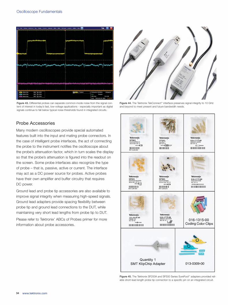
Oscilloscope Fundamentals
Probe Accessories
Many modern oscilloscopes provide special automated features built into the input and mating probe connectors. Inthe case of intelligent probe interfaces, the act of connectingthe probe to the instrument notifies the oscilloscope aboutthe probe’s attenuation factor, which in turn scales the displayso that the probe’s attenuation is figured into the readout onthe screen. Some probe interfaces also recognize the type of probe – that is, passive, active or current. The interfacemay act as a DC power source for probes. Active probeshave their own amplifier and buffer circuitry that requires DC power.
Ground lead and probe tip accessories are also available toimprove signal integrity when measuring high-speed signals.Ground lead adapters provide spacing flexibility betweenprobe tip and ground lead connections to the DUT, whilemaintaining very short lead lengths from probe tip to DUT.
Please refer to Tektronix’ ABCs of Probes primer for moreinformation about probe accessories.
34 www.tektronix.com
Figure 44. The Tektronix TekConnectTM interface preserves signal integrity to 10 GHzand beyond to meet present and future bandwidth needs.
Figure 45. The Tektronix SF200A and SF500 Series SureFootTM adapters provided reli-able short-lead length probe tip connection to a specific pin on an integrated circuit.
Figure 43. Differential probes can separate common-mode noise from the signal con-tent of interest in today’s fast, low-voltage applications - especially important as digitalsignals continue to fall below typical noise thresholds found in integrated circuits.
03W-8605-4_edu.qxd 3/31/09 1:55 PM Page 34
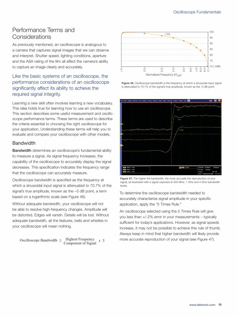
Oscilloscope Fundamentals
35www.tektronix.com
Performance Terms andConsiderationsAs previously mentioned, an oscilloscope is analogous to a camera that captures signal images that we can observe and interpret. Shutter speed, lighting conditions, aperture and the ASA rating of the film all affect the camera’s ability to capture an image clearly and accurately.
Like the basic systems of an oscilloscope, theperformance considerations of an oscilloscopesignificantly affect its ability to achieve therequired signal integrity.
Learning a new skill often involves learning a new vocabulary.This idea holds true for learning how to use an oscilloscope.This section describes some useful measurement and oscillo-scope performance terms. These terms are used to describethe criteria essential to choosing the right oscilloscope foryour application. Understanding these terms will help you toevaluate and compare your oscilloscope with other models.
Bandwidth
Bandwidth determines an oscilloscope’s fundamental abilityto measure a signal. As signal frequency increases, the capability of the oscilloscope to accurately display the signaldecreases. This specification indicates the frequency rangethat the oscilloscope can accurately measure.
Oscilloscope bandwidth is specified as the frequency atwhich a sinusoidal input signal is attenuated to 70.7% of thesignal’s true amplitude, known as the –3 dB point, a termbased on a logarithmic scale (see Figure 46).
Without adequate bandwidth, your oscilloscope will not be able to resolve high-frequency changes. Amplitude will be distorted. Edges will vanish. Details will be lost. Without adequate bandwidth, all the features, bells and whistles inyour oscilloscope will mean nothing.
To determine the oscilloscope bandwidth needed to accurately characterize signal amplitude in your specific application, apply the “5 Times Rule.”
An oscilloscope selected using the 5 Times Rule will give you less than +/-2% error in your measurements – typicallysufficient for today’s applications. However, as signal speedsincrease, it may not be possible to achieve this rule of thumb.Always keep in mind that higher bandwidth will likely providemore accurate reproduction of your signal (see Figure 47).
0.1
0.2
0.3
0.4
0.9
0.8
0.7
0.6
0.5
1.0
70 (-3dB)
75
80
85
90
95
100
Normalized Frequency (f/f )3dB
3%
Figure 46. Oscilloscope bandwidth is the frequency at which a sinusoidal input signalis attenuated to 70.7% of the signal’s true amplitude, known as the -3 dB point.
≥ x 5Oscilloscope Bandwidth Highest FrequencyComponent of Signal
Figure 47. The higher the bandwidth, the more accurate the reproduction of your signal, as illustrated with a signal captured at 250 MHz, 1 GHz and 4 GHz bandwidthlevels.
03W-8605-4_edu.qxd 3/31/09 1:55 PM Page 35
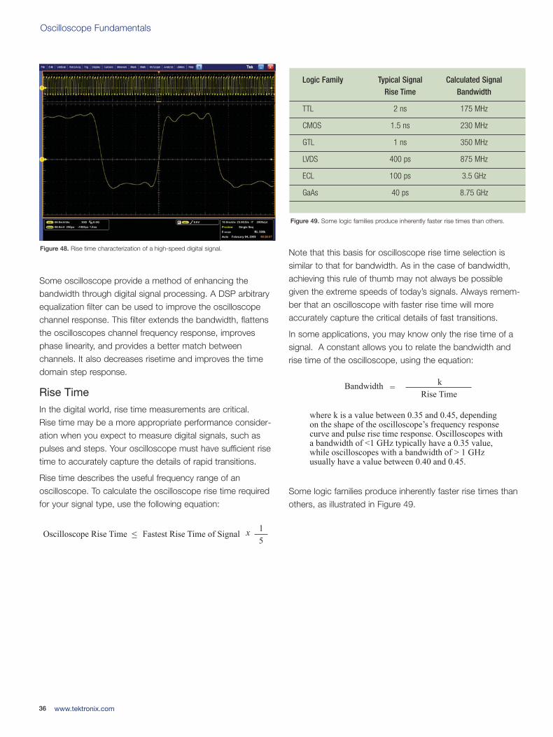
Oscilloscope Fundamentals
Some oscilloscope provide a method of enhancing the bandwidth through digital signal processing. A DSP arbitraryequalization filter can be used to improve the oscilloscopechannel response. This filter extends the bandwidth, flattensthe oscilloscopes channel frequency response, improvesphase linearity, and provides a better match between channels. It also decreases risetime and improves the timedomain step response.
Rise Time
In the digital world, rise time measurements are critical. Rise time may be a more appropriate performance consider-ation when you expect to measure digital signals, such aspulses and steps. Your oscilloscope must have sufficient risetime to accurately capture the details of rapid transitions.
Rise time describes the useful frequency range of an oscilloscope. To calculate the oscilloscope rise time requiredfor your signal type, use the following equation:
Note that this basis for oscilloscope rise time selection is similar to that for bandwidth. As in the case of bandwidth,achieving this rule of thumb may not always be possiblegiven the extreme speeds of today’s signals. Always remem-ber that an oscilloscope with faster rise time will more accurately capture the critical details of fast transitions.
In some applications, you may know only the rise time of asignal. A constant allows you to relate the bandwidth andrise time of the oscilloscope, using the equation:
Some logic families produce inherently faster rise times thanothers, as illustrated in Figure 49.
36 www.tektronix.com
≤ x
Oscilloscope Rise Time Fastest Rise Time of Signal51
Figure 48. Rise time characterization of a high-speed digital signal.
Logic Family Typical Signal Calculated SignalRise Time Bandwidth
TTL 2 ns 175 MHz
CMOS 1.5 ns 230 MHz
GTL 1 ns 350 MHz
LVDS 400 ps 875 MHz
ECL 100 ps 3.5 GHz
GaAs 40 ps 8.75 GHz
Figure 49. Some logic families produce inherently faster rise times than others.
where k is a value between 0.35 and 0.45, depending on the shape of the oscilloscope’s frequency response curve and pulse rise time response. Oscilloscopes with a bandwidth of <1 GHz typically have a 0.35 value, while oscilloscopes with a bandwidth of > 1 GHz usually have a value between 0.40 and 0.45.
=kBandwidth
Rise Time
03W-8605-4_edu.qxd 3/31/09 1:55 PM Page 36
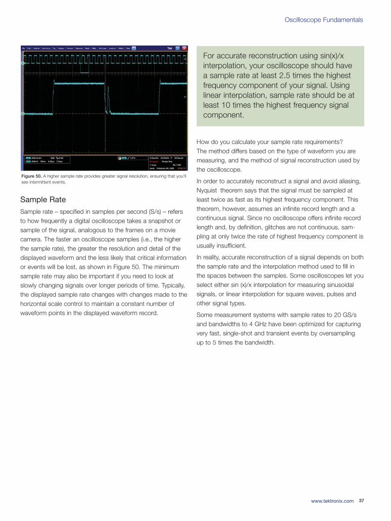
Oscilloscope Fundamentals
37www.tektronix.com
Sample Rate
Sample rate – specified in samples per second (S/s) – refersto how frequently a digital oscilloscope takes a snapshot orsample of the signal, analogous to the frames on a moviecamera. The faster an oscilloscope samples (i.e., the higherthe sample rate), the greater the resolution and detail of thedisplayed waveform and the less likely that critical informationor events will be lost, as shown in Figure 50. The minimumsample rate may also be important if you need to look atslowly changing signals over longer periods of time. Typically,the displayed sample rate changes with changes made to thehorizontal scale control to maintain a constant number ofwaveform points in the displayed waveform record.
How do you calculate your sample rate requirements? The method differs based on the type of waveform you aremeasuring, and the method of signal reconstruction used bythe oscilloscope.
In order to accurately reconstruct a signal and avoid aliasing,Nyquist theorem says that the signal must be sampled atleast twice as fast as its highest frequency component. Thistheorem, however, assumes an infinite record length and acontinuous signal. Since no oscilloscope offers infinite recordlength and, by definition, glitches are not continuous, sam-pling at only twice the rate of highest frequency component isusually insufficient.
In reality, accurate reconstruction of a signal depends on boththe sample rate and the interpolation method used to fill inthe spaces between the samples. Some oscilloscopes let youselect either sin (x)/x interpolation for measuring sinusoidalsignals, or linear interpolation for square waves, pulses andother signal types.
Some measurement systems with sample rates to 20 GS/sand bandwidths to 4 GHz have been optimized for capturingvery fast, single-shot and transient events by oversamplingup to 5 times the bandwidth.
Figure 50. A higher sample rate provides greater signal resolution, ensuring that you’llsee intermittent events.
For accurate reconstruction using sin(x)/xinterpolation, your oscilloscope should havea sample rate at least 2.5 times the highestfrequency component of your signal. Usinglinear interpolation, sample rate should be atleast 10 times the highest frequency signalcomponent.
03W-8605-4_edu.qxd 3/31/09 1:55 PM Page 37
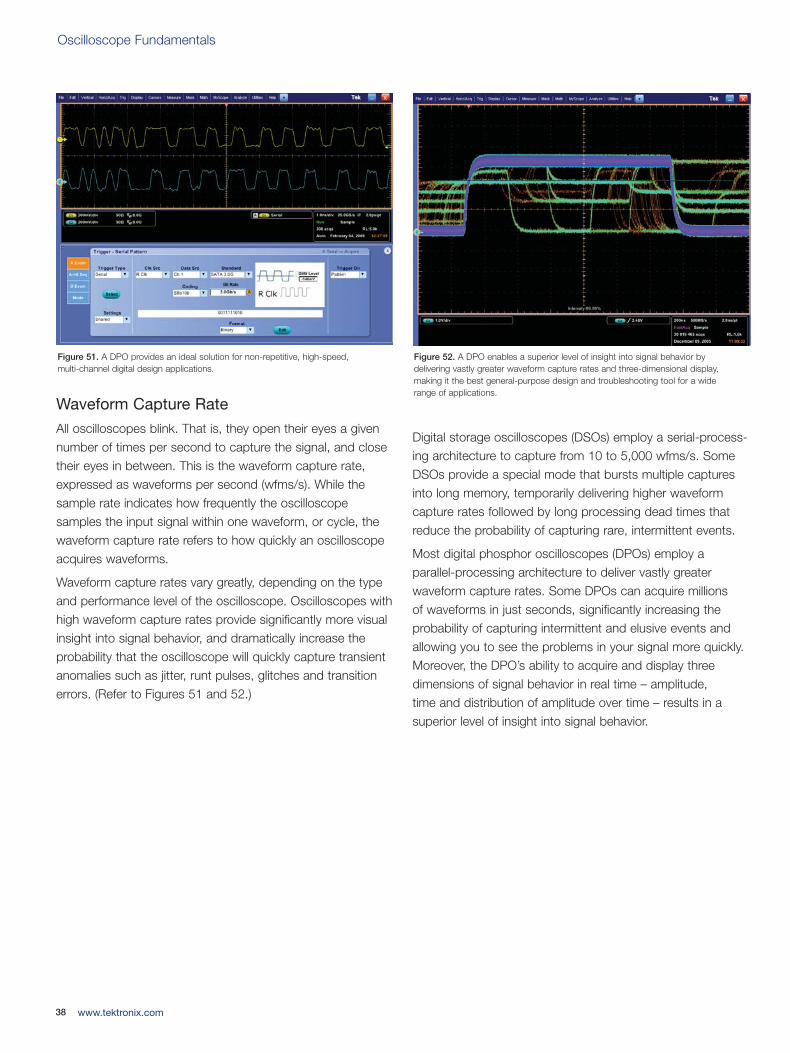
Oscilloscope Fundamentals
Waveform Capture Rate
All oscilloscopes blink. That is, they open their eyes a givennumber of times per second to capture the signal, and closetheir eyes in between. This is the waveform capture rate,expressed as waveforms per second (wfms/s). While thesample rate indicates how frequently the oscilloscope samples the input signal within one waveform, or cycle, thewaveform capture rate refers to how quickly an oscilloscopeacquires waveforms.
Waveform capture rates vary greatly, depending on the typeand performance level of the oscilloscope. Oscilloscopes withhigh waveform capture rates provide significantly more visualinsight into signal behavior, and dramatically increase theprobability that the oscilloscope will quickly capture transientanomalies such as jitter, runt pulses, glitches and transitionerrors. (Refer to Figures 51 and 52.)
Digital storage oscilloscopes (DSOs) employ a serial-process-ing architecture to capture from 10 to 5,000 wfms/s. SomeDSOs provide a special mode that bursts multiple capturesinto long memory, temporarily delivering higher waveformcapture rates followed by long processing dead times thatreduce the probability of capturing rare, intermittent events.
Most digital phosphor oscilloscopes (DPOs) employ a parallel-processing architecture to deliver vastly greater waveform capture rates. Some DPOs can acquire millions of waveforms in just seconds, significantly increasing theprobability of capturing intermittent and elusive events andallowing you to see the problems in your signal more quickly.Moreover, the DPO’s ability to acquire and display threedimensions of signal behavior in real time – amplitude, time and distribution of amplitude over time – results in asuperior level of insight into signal behavior.
38 www.tektronix.com
Figure 52. A DPO enables a superior level of insight into signal behavior by delivering vastly greater waveform capture rates and three-dimensional display, making it the best general-purpose design and troubleshooting tool for a wide range of applications.
Figure 51. A DPO provides an ideal solution for non-repetitive, high-speed, multi-channel digital design applications.
03W-8605-4_edu.qxd 3/31/09 1:55 PM Page 38
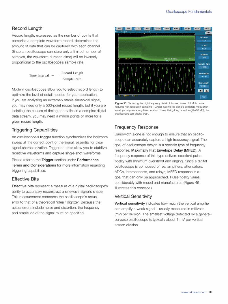
Oscilloscope Fundamentals
39www.tektronix.com
Record Length
Record length, expressed as the number of points that comprise a complete waveform record, determines theamount of data that can be captured with each channel.Since an oscilloscope can store only a limited number ofsamples, the waveform duration (time) will be inversely proportional to the oscilloscope’s sample rate.
Modern oscilloscopes allow you to select record length tooptimize the level of detail needed for your application. If you are analyzing an extremely stable sinusoidal signal, you may need only a 500-point record length, but if you areisolating the causes of timing anomalies in a complex digitaldata stream, you may need a million points or more for agiven record length.
Triggering Capabilities
An oscilloscope’s trigger function synchronizes the horizontalsweep at the correct point of the signal, essential for clearsignal characterization. Trigger controls allow you to stabilizerepetitive waveforms and capture single-shot waveforms.
Please refer to the Trigger section under Performance
Terms and Considerations for more information regardingtriggering capabilities.
Effective Bits
Effective bits represent a measure of a digital oscilloscope'sability to accurately reconstruct a sinewave signal’s shape.This measurement compares the oscilloscope's actual error to that of a theoretical “ideal” digitizer. Because theactual errors include noise and distortion, the frequency and amplitude of the signal must be specified.
Frequency Response
Bandwidth alone is not enough to ensure that an oscillo-scope can accurately capture a high frequency signal. Thegoal of oscilloscope design is a specific type of frequencyresponse: Maximally Flat Envelope Delay (MFED). A frequency response of this type delivers excellent pulse fidelity with minimum overshoot and ringing. Since a digitaloscilloscope is composed of real amplifiers, attenuators,ADCs, interconnects, and relays, MFED response is a goal that can only be approached. Pulse fidelity varies considerably with model and manufacturer. (Figure 46 illustrates this concept.)
Vertical Sensitivity
Vertical sensitivity indicates how much the vertical amplifiercan amplify a weak signal – usually measured in millivolts(mV) per division. The smallest voltage detected by a general-purpose oscilloscope is typically about 1 mV per verticalscreen division.
=Record Length
Time IntervalSample Rate
Figure 53. Capturing the high frequency detail of this modulated 85 MHz carrierrequires high resolution sampling (100 ps). Seeing the signal’s complete modulationenvelope requires a long time duration (1 ms). Using long record length (10 MB), theoscilloscope can display both.
03W-8605-4_edu.qxd 3/31/09 1:56 PM Page 39
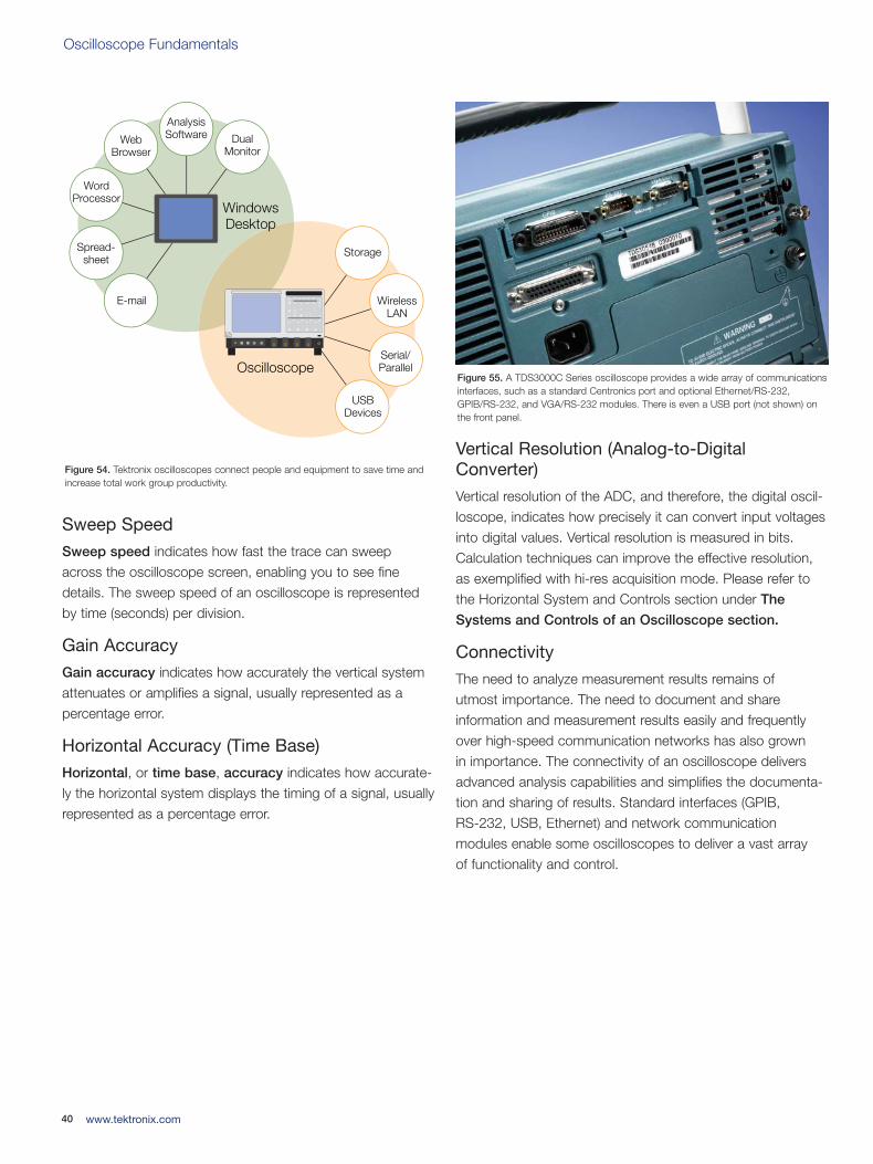
Oscilloscope Fundamentals
Sweep Speed
Sweep speed indicates how fast the trace can sweepacross the oscilloscope screen, enabling you to see finedetails. The sweep speed of an oscilloscope is representedby time (seconds) per division.
Gain Accuracy
Gain accuracy indicates how accurately the vertical systemattenuates or amplifies a signal, usually represented as a percentage error.
Horizontal Accuracy (Time Base)
Horizontal, or time base, accuracy indicates how accurate-ly the horizontal system displays the timing of a signal, usuallyrepresented as a percentage error.
Vertical Resolution (Analog-to-DigitalConverter)
Vertical resolution of the ADC, and therefore, the digital oscil-loscope, indicates how precisely it can convert input voltagesinto digital values. Vertical resolution is measured in bits.Calculation techniques can improve the effective resolution,as exemplified with hi-res acquisition mode. Please refer tothe Horizontal System and Controls section under The
Systems and Controls of an Oscilloscope section.
Connectivity
The need to analyze measurement results remains of utmost importance. The need to document and share information and measurement results easily and frequentlyover high-speed communication networks has also grown in importance. The connectivity of an oscilloscope deliversadvanced analysis capabilities and simplifies the documenta-tion and sharing of results. Standard interfaces (GPIB, RS-232, USB, Ethernet) and network communication modules enable some oscilloscopes to deliver a vast array of functionality and control.
40 www.tektronix.com
AnalysisSoftware Dual
Monitor
WindowsDesktop
WebBrowser
WordProcessor
Spread-sheet
Storage
Serial/Parallel
WirelessLAN
USBDevices
Oscilloscope
Figure 54. Tektronix oscilloscopes connect people and equipment to save time andincrease total work group productivity.
Figure 55. A TDS3000C Series oscilloscope provides a wide array of communicationsinterfaces, such as a standard Centronics port and optional Ethernet/RS-232,GPIB/RS-232, and VGA/RS-232 modules. There is even a USB port (not shown) onthe front panel.
03W-8605-4_edu.qxd 3/31/09 1:56 PM Page 40
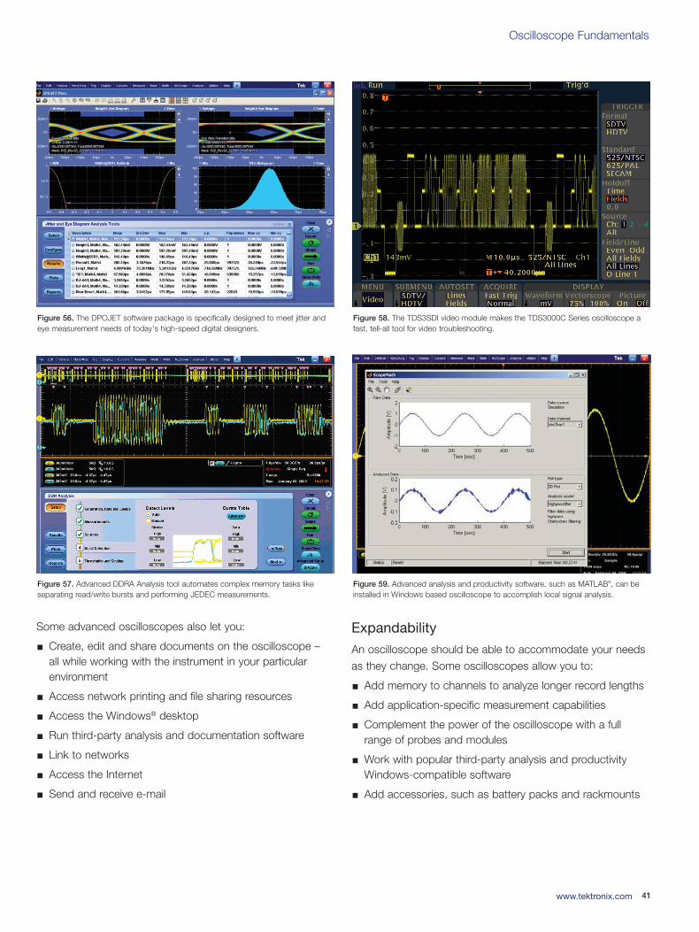
Oscilloscope Fundamentals
41www.tektronix.com
Some advanced oscilloscopes also let you:
Create, edit and share documents on the oscilloscope –all while working with the instrument in your particular environment
Access network printing and file sharing resources
Access the Windows® desktop
Run third-party analysis and documentation software
Link to networks
Access the Internet
Send and receive e-mail
Expandability
An oscilloscope should be able to accommodate your needsas they change. Some oscilloscopes allow you to:
Add memory to channels to analyze longer record lengths
Add application-specific measurement capabilities
Complement the power of the oscilloscope with a fullrange of probes and modules
Work with popular third-party analysis and productivityWindows-compatible software
Add accessories, such as battery packs and rackmounts
Figure 56. The DPOJET software package is specifically designed to meet jitter andeye measurement needs of today's high-speed digital designers.
Figure 57. Advanced DDRA Analysis tool automates complex memory tasks like separating read/write bursts and performing JEDEC measurements.
Figure 58. The TDS3SDI video module makes the TDS3000C Series oscilloscope afast, tell-all tool for video troubleshooting.
Figure 59. Advanced analysis and productivity software, such as MATLAB®, can beinstalled in Windows based oscilloscope to accomplish local signal analysis.
03W-8605-4_edu.qxd 3/31/09 1:56 PM Page 41
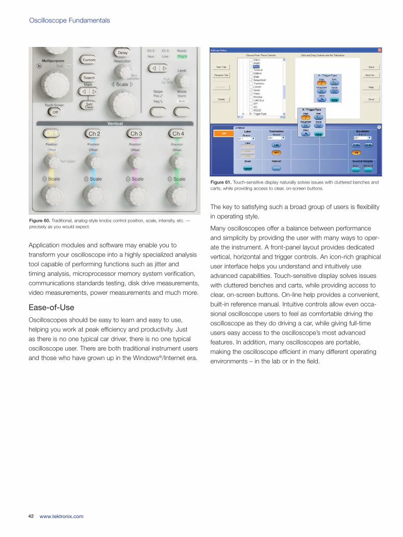
Oscilloscope Fundamentals
Application modules and software may enable you to transform your oscilloscope into a highly specialized analysistool capable of performing functions such as jitter and timing analysis, microprocessor memory system verification,communications standards testing, disk drive measurements,video measurements, power measurements and much more.
Ease-of-Use
Oscilloscopes should be easy to learn and easy to use, helping you work at peak efficiency and productivity. Just as there is no one typical car driver, there is no one typical oscilloscope user. There are both traditional instrument usersand those who have grown up in the Windows®/Internet era.
The key to satisfying such a broad group of users is flexibilityin operating style.
Many oscilloscopes offer a balance between performanceand simplicity by providing the user with many ways to oper-ate the instrument. A front-panel layout provides dedicatedvertical, horizontal and trigger controls. An icon-rich graphicaluser interface helps you understand and intuitively useadvanced capabilities. Touch-sensitive display solves issueswith cluttered benches and carts, while providing access toclear, on-screen buttons. On-line help provides a convenient,built-in reference manual. Intuitive controls allow even occa-sional oscilloscope users to feel as comfortable driving theoscilloscope as they do driving a car, while giving full-timeusers easy access to the oscilloscope’s most advanced features. In addition, many oscilloscopes are portable, making the oscilloscope efficient in many different operatingenvironments – in the lab or in the field.
42 www.tektronix.com
Figure 60. Traditional, analog-style knobs control position, scale, intensity, etc. — precisely as you would expect.
Figure 61. Touch-sensitive display naturally solves issues with cluttered benches andcarts, while providing access to clear, on-screen buttons.
03W-8605-4_edu.qxd 3/31/09 1:56 PM Page 42
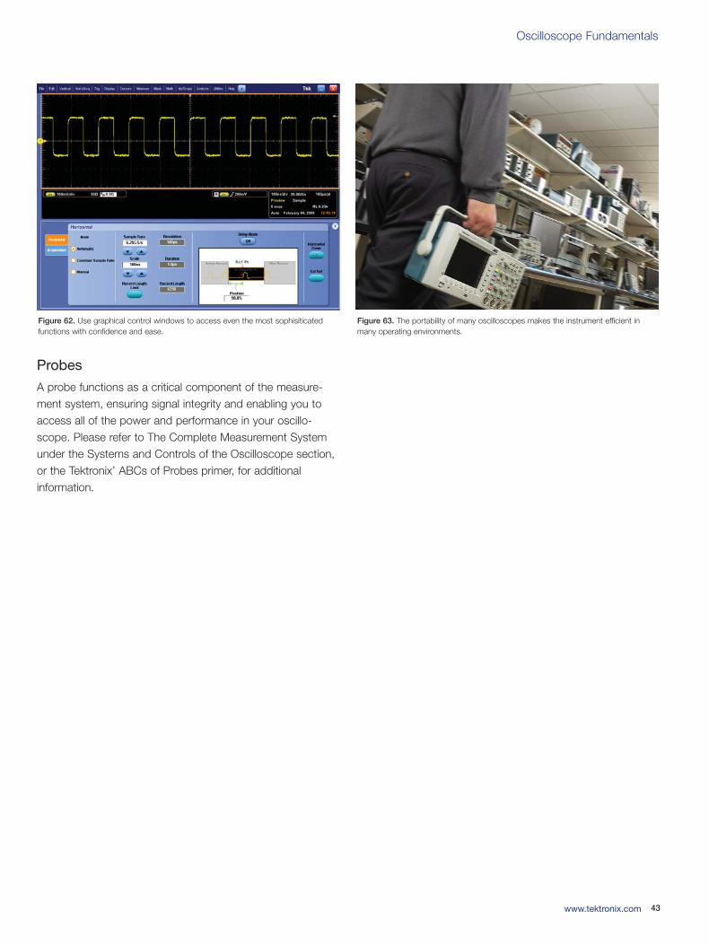
Oscilloscope Fundamentals
43www.tektronix.com
Probes
A probe functions as a critical component of the measure-ment system, ensuring signal integrity and enabling you toaccess all of the power and performance in your oscillo-scope. Please refer to The Complete Measurement Systemunder the Systems and Controls of the Oscilloscope section,or the Tektronix’ ABCs of Probes primer, for additional information.
Figure 62. Use graphical control windows to access even the most sophisiticatedfunctions with confidence and ease.
Figure 63. The portability of many oscilloscopes makes the instrument efficient inmany operating environments.
03W-8605-4_edu.qxd 3/31/09 1:56 PM Page 43
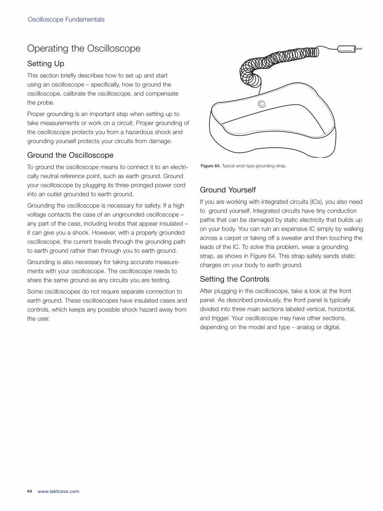
Oscilloscope Fundamentals
Operating the Oscilloscope
Setting Up
This section briefly describes how to set up and start using an oscilloscope – specifically, how to ground the oscilloscope, calibrate the oscilloscope, and compensate the probe.
Proper grounding is an important step when setting up totake measurements or work on a circuit. Proper grounding ofthe oscilloscope protects you from a hazardous shock andgrounding yourself protects your circuits from damage.
Ground the Oscilloscope
To ground the oscilloscope means to connect it to an electri-cally neutral reference point, such as earth ground. Groundyour oscilloscope by plugging its three-pronged power cordinto an outlet grounded to earth ground.
Grounding the oscilloscope is necessary for safety. If a highvoltage contacts the case of an ungrounded oscilloscope –any part of the case, including knobs that appear insulated –it can give you a shock. However, with a properly groundedoscilloscope, the current travels through the grounding pathto earth ground rather than through you to earth ground.
Grounding is also necessary for taking accurate measure-ments with your oscilloscope. The oscilloscope needs toshare the same ground as any circuits you are testing.
Some oscilloscopes do not require separate connection toearth ground. These oscilloscopes have insulated cases andcontrols, which keeps any possible shock hazard away fromthe user.
Ground Yourself
If you are working with integrated circuits (ICs), you also needto ground yourself. Integrated circuits have tiny conductionpaths that can be damaged by static electricity that builds upon your body. You can ruin an expensive IC simply by walkingacross a carpet or taking off a sweater and then touching theleads of the IC. To solve this problem, wear a groundingstrap, as shows in Figure 64. This strap safely sends staticcharges on your body to earth ground.
Setting the Controls
After plugging in the oscilloscope, take a look at the frontpanel. As described previously, the front panel is typicallydivided into three main sections labeled vertical, horizontal,and trigger. Your oscilloscope may have other sections,depending on the model and type – analog or digital.
44 www.tektronix.com
C
Figure 64. Typical wrist-type grounding strap.
03W-8605-4_edu.qxd 3/31/09 1:56 PM Page 44
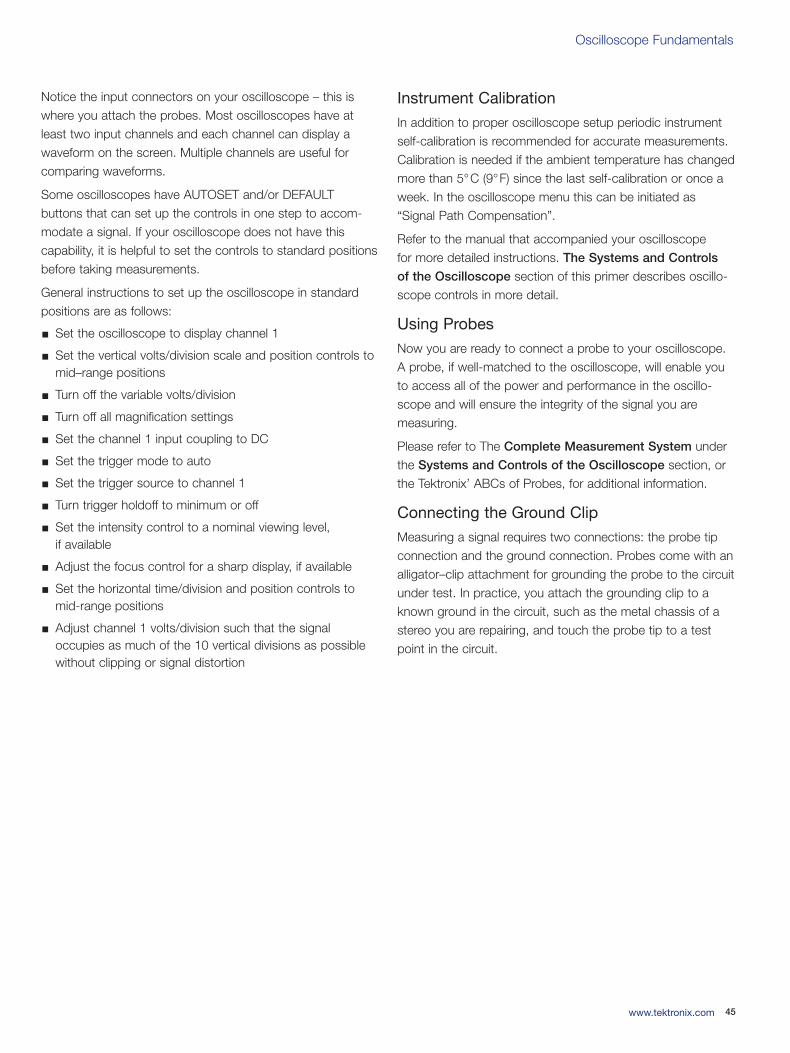
Oscilloscope Fundamentals
45www.tektronix.com
Notice the input connectors on your oscilloscope – this iswhere you attach the probes. Most oscilloscopes have atleast two input channels and each channel can display awaveform on the screen. Multiple channels are useful forcomparing waveforms.
Some oscilloscopes have AUTOSET and/or DEFAULT buttons that can set up the controls in one step to accom-modate a signal. If your oscilloscope does not have thiscapability, it is helpful to set the controls to standard positionsbefore taking measurements.
General instructions to set up the oscilloscope in standardpositions are as follows:
Set the oscilloscope to display channel 1
Set the vertical volts/division scale and position controls tomid–range positions
Turn off the variable volts/division
Turn off all magnification settings
Set the channel 1 input coupling to DC
Set the trigger mode to auto
Set the trigger source to channel 1
Turn trigger holdoff to minimum or off
Set the intensity control to a nominal viewing level, if available
Adjust the focus control for a sharp display, if available
Set the horizontal time/division and position controls tomid-range positions
Adjust channel 1 volts/division such that the signal occupies as much of the 10 vertical divisions as possiblewithout clipping or signal distortion
Instrument Calibration
In addition to proper oscilloscope setup periodic instrumentself-calibration is recommended for accurate measurements.Calibration is needed if the ambient temperature has changedmore than 5°C (9°F) since the last self-calibration or once aweek. In the oscilloscope menu this can be initiated as“Signal Path Compensation”.
Refer to the manual that accompanied your oscilloscope for more detailed instructions. The Systems and Controls
of the Oscilloscope section of this primer describes oscillo-scope controls in more detail.
Using Probes
Now you are ready to connect a probe to your oscilloscope.A probe, if well-matched to the oscilloscope, will enable youto access all of the power and performance in the oscillo-scope and will ensure the integrity of the signal you aremeasuring.
Please refer to The Complete Measurement System underthe Systems and Controls of the Oscilloscope section, orthe Tektronix’ ABCs of Probes, for additional information.
Connecting the Ground Clip
Measuring a signal requires two connections: the probe tipconnection and the ground connection. Probes come with analligator–clip attachment for grounding the probe to the circuitunder test. In practice, you attach the grounding clip to aknown ground in the circuit, such as the metal chassis of astereo you are repairing, and touch the probe tip to a testpoint in the circuit.
03W-8605-4_edu.qxd 3/31/09 1:56 PM Page 45
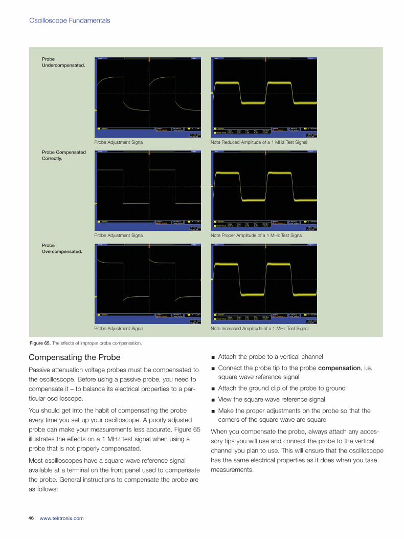
Oscilloscope Fundamentals
Compensating the Probe
Passive attenuation voltage probes must be compensated tothe oscilloscope. Before using a passive probe, you need tocompensate it – to balance its electrical properties to a par-ticular oscilloscope.
You should get into the habit of compensating the probeevery time you set up your oscilloscope. A poorly adjustedprobe can make your measurements less accurate. Figure 65illustrates the effects on a 1 MHz test signal when using aprobe that is not properly compensated.
Most oscilloscopes have a square wave reference signalavailable at a terminal on the front panel used to compensatethe probe. General instructions to compensate the probe areas follows:
Attach the probe to a vertical channel
Connect the probe tip to the probe compensation, i.e.square wave reference signal
Attach the ground clip of the probe to ground
View the square wave reference signal
Make the proper adjustments on the probe so that thecorners of the square wave are square
When you compensate the probe, always attach any acces-sory tips you will use and connect the probe to the verticalchannel you plan to use. This will ensure that the oscilloscopehas the same electrical properties as it does when you takemeasurements.
46 www.tektronix.com
Figure 65. The effects of improper probe compensation.
ProbeUndercompensated.
Probe Adjustment Signal Note Reduced Amplitude of a 1 MHz Test Signal
Probe CompensatedCorrectly.
Probe Adjustment Signal Note Proper Amplitude of a 1 MHz Test Signal
ProbeOvercompensated.
Probe Adjustment Signal Note Increased Amplitude of a 1 MHz Test Signal
03W-8605-4_edu.qxd 3/31/09 1:56 PM Page 46
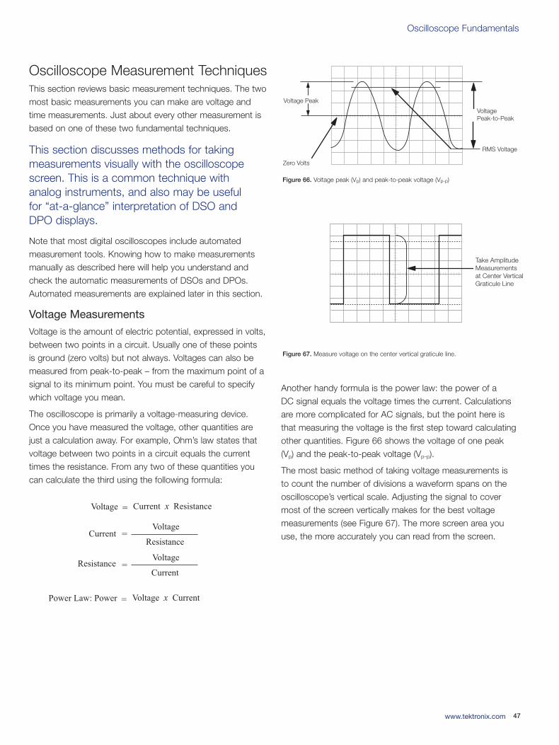
Oscilloscope Fundamentals
47www.tektronix.com
Oscilloscope Measurement TechniquesThis section reviews basic measurement techniques. The twomost basic measurements you can make are voltage andtime measurements. Just about every other measurement isbased on one of these two fundamental techniques.
This section discusses methods for takingmeasurements visually with the oscilloscopescreen. This is a common technique with analog instruments, and also may be useful for “at-a-glance” interpretation of DSO and DPO displays.
Note that most digital oscilloscopes include automatedmeasurement tools. Knowing how to make measurementsmanually as described here will help you understand andcheck the automatic measurements of DSOs and DPOs.Automated measurements are explained later in this section.
Voltage Measurements
Voltage is the amount of electric potential, expressed in volts,between two points in a circuit. Usually one of these points is ground (zero volts) but not always. Voltages can also bemeasured from peak-to-peak – from the maximum point of asignal to its minimum point. You must be careful to specifywhich voltage you mean.
The oscilloscope is primarily a voltage-measuring device.Once you have measured the voltage, other quantities arejust a calculation away. For example, Ohm’s law states thatvoltage between two points in a circuit equals the currenttimes the resistance. From any two of these quantities youcan calculate the third using the following formula:
Another handy formula is the power law: the power of a DC signal equals the voltage times the current. Calculationsare more complicated for AC signals, but the point here isthat measuring the voltage is the first step toward calculatingother quantities. Figure 66 shows the voltage of one peak (Vp) and the peak-to-peak voltage (Vp–p).
The most basic method of taking voltage measurements is to count the number of divisions a waveform spans on theoscilloscope’s vertical scale. Adjusting the signal to covermost of the screen vertically makes for the best voltagemeasurements (see Figure 67). The more screen area youuse, the more accurately you can read from the screen.
Voltage Peak
Zero Volts
VoltagePeak-to-Peak
RMS Voltage
Figure 66. Voltage peak (Vp) and peak-to-peak voltage (Vp-p)
Take AmplitudeMeasurementsat Center VerticalGraticule Line
Figure 67. Measure voltage on the center vertical graticule line.
= Current x ResistanceVoltage
= Voltage x CurrentPower Law: Power
=Voltage
CurrentResistance
=Voltage
ResistanceCurrent
03W-8605-4_edu.qxd 3/31/09 1:56 PM Page 47
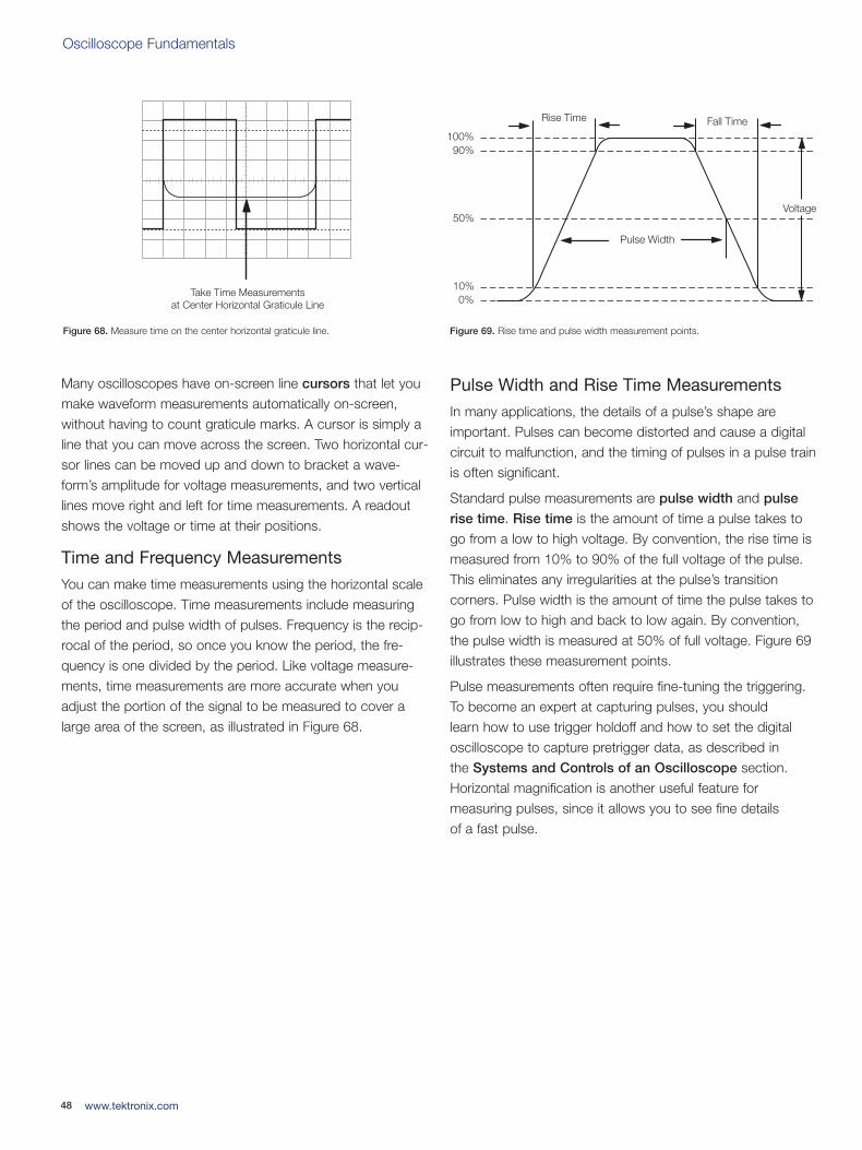
Oscilloscope Fundamentals
Many oscilloscopes have on-screen line cursors that let youmake waveform measurements automatically on-screen,without having to count graticule marks. A cursor is simply aline that you can move across the screen. Two horizontal cur-sor lines can be moved up and down to bracket a wave-form’s amplitude for voltage measurements, and two verticallines move right and left for time measurements. A readoutshows the voltage or time at their positions.
Time and Frequency Measurements
You can make time measurements using the horizontal scaleof the oscilloscope. Time measurements include measuringthe period and pulse width of pulses. Frequency is the recip-rocal of the period, so once you know the period, the fre-quency is one divided by the period. Like voltage measure-ments, time measurements are more accurate when youadjust the portion of the signal to be measured to cover alarge area of the screen, as illustrated in Figure 68.
Pulse Width and Rise Time Measurements
In many applications, the details of a pulse’s shape areimportant. Pulses can become distorted and cause a digitalcircuit to malfunction, and the timing of pulses in a pulse trainis often significant.
Standard pulse measurements are pulse width and pulse
rise time. Rise time is the amount of time a pulse takes togo from a low to high voltage. By convention, the rise time ismeasured from 10% to 90% of the full voltage of the pulse.This eliminates any irregularities at the pulse’s transition corners. Pulse width is the amount of time the pulse takes togo from low to high and back to low again. By convention,the pulse width is measured at 50% of full voltage. Figure 69illustrates these measurement points.
Pulse measurements often require fine-tuning the triggering.To become an expert at capturing pulses, you should learn how to use trigger holdoff and how to set the digitaloscilloscope to capture pretrigger data, as described in the Systems and Controls of an Oscilloscope section.Horizontal magnification is another useful feature for measuring pulses, since it allows you to see fine details of a fast pulse.
48 www.tektronix.com
Take Time Measurementsat Center Horizontal Graticule Line
Figure 68. Measure time on the center horizontal graticule line.
100%90%
50%
10%0%
Rise Time Fall Time
Voltage
Pulse Width
Figure 69. Rise time and pulse width measurement points.
03W-8605-4_edu.qxd 3/31/09 1:56 PM Page 48
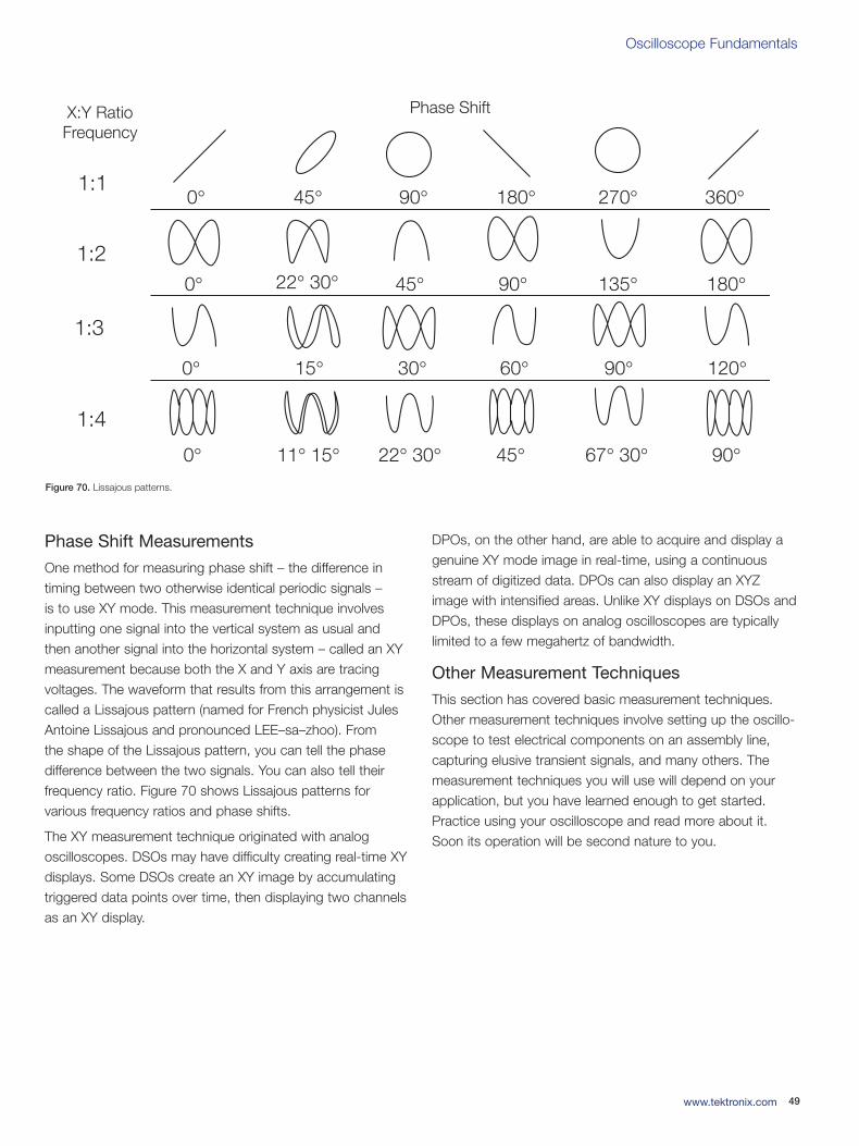
Oscilloscope Fundamentals
49www.tektronix.com
Phase Shift Measurements
One method for measuring phase shift – the difference in timing between two otherwise identical periodic signals – is to use XY mode. This measurement technique involvesinputting one signal into the vertical system as usual and then another signal into the horizontal system – called an XYmeasurement because both the X and Y axis are tracing voltages. The waveform that results from this arrangement iscalled a Lissajous pattern (named for French physicist JulesAntoine Lissajous and pronounced LEE–sa–zhoo). From the shape of the Lissajous pattern, you can tell the phase difference between the two signals. You can also tell their frequency ratio. Figure 70 shows Lissajous patterns for various frequency ratios and phase shifts.
The XY measurement technique originated with analog oscilloscopes. DSOs may have difficulty creating real-time XYdisplays. Some DSOs create an XY image by accumulatingtriggered data points over time, then displaying two channelsas an XY display.
DPOs, on the other hand, are able to acquire and display agenuine XY mode image in real-time, using a continuousstream of digitized data. DPOs can also display an XYZimage with intensified areas. Unlike XY displays on DSOs andDPOs, these displays on analog oscilloscopes are typicallylimited to a few megahertz of bandwidth.
Other Measurement Techniques
This section has covered basic measurement techniques.Other measurement techniques involve setting up the oscillo-scope to test electrical components on an assembly line,capturing elusive transient signals, and many others. Themeasurement techniques you will use will depend on yourapplication, but you have learned enough to get started.Practice using your oscilloscope and read more about it.Soon its operation will be second nature to you.
0° 45° 90° 180° 270° 360°
0° 22° 30° 45° 90° 135° 180°
0° 15° 30° 60° 90° 120°
0° 11° 15° 22° 30° 45° 67° 30° 90°
Phase Shift
1:1
1:2
1:3
1:4
X:Y RatioFrequency
Figure 70. Lissajous patterns.
03W-8605-4_edu.qxd 3/31/09 1:56 PM Page 49
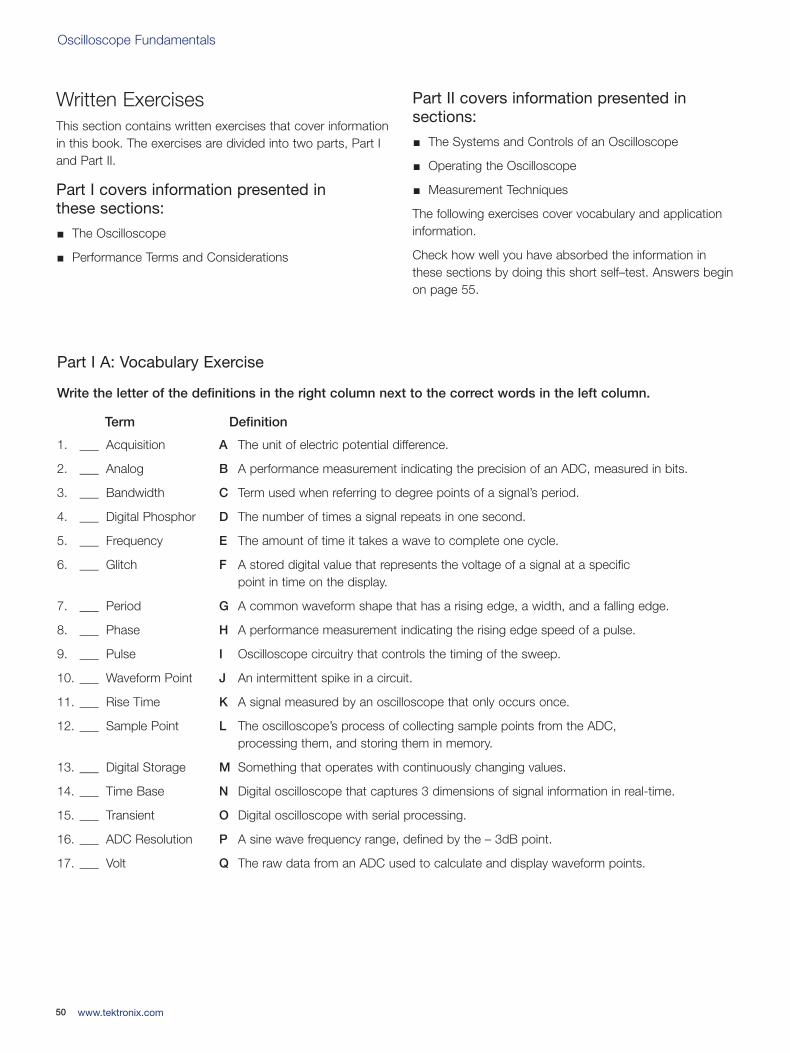
Oscilloscope Fundamentals
Written ExercisesThis section contains written exercises that cover informationin this book. The exercises are divided into two parts, Part Iand Part II.
Part I covers information presented in these sections:
The Oscilloscope
Performance Terms and Considerations
Part II covers information presented in sections:
The Systems and Controls of an Oscilloscope
Operating the Oscilloscope
Measurement Techniques
The following exercises cover vocabulary and applicationinformation.
Check how well you have absorbed the information in these sections by doing this short self–test. Answers beginon page 55.
50 www.tektronix.com
Part I A: Vocabulary Exercise
Write the letter of the definitions in the right column next to the correct words in the left column.
Term Definition
1. ___ Acquisition A The unit of electric potential difference.
2. ___ Analog B A performance measurement indicating the precision of an ADC, measured in bits.
3. ___ Bandwidth C Term used when referring to degree points of a signal’s period.
4. ___ Digital Phosphor D The number of times a signal repeats in one second.
5. ___ Frequency E The amount of time it takes a wave to complete one cycle.
6. ___ Glitch F A stored digital value that represents the voltage of a signal at a specific point in time on the display.
7. ___ Period G A common waveform shape that has a rising edge, a width, and a falling edge.
8. ___ Phase H A performance measurement indicating the rising edge speed of a pulse.
9. ___ Pulse I Oscilloscope circuitry that controls the timing of the sweep.
10. ___ Waveform Point J An intermittent spike in a circuit.
11. ___ Rise Time K A signal measured by an oscilloscope that only occurs once.
12. ___ Sample Point L The oscilloscope’s process of collecting sample points from the ADC, processing them, and storing them in memory.
13. ___ Digital Storage M Something that operates with continuously changing values.
14. ___ Time Base N Digital oscilloscope that captures 3 dimensions of signal information in real-time.
15. ___ Transient O Digital oscilloscope with serial processing.
16. ___ ADC Resolution P A sine wave frequency range, defined by the – 3dB point.
17. ___ Volt Q The raw data from an ADC used to calculate and display waveform points.
03W-8605-4_edu.qxd 3/31/09 1:56 PM Page 50
Oscilloscope Fundamentals
51www.tektronix.com
Part I B: Application Exercise
Circle the best answers for each statement. Some statements have more than one right answer.
1. With an oscilloscope you can:
a. Calculate the frequency of a signal.
b. Find malfunctioning electrical components.
c. Analyze signal details.
d. All the above.
2. The difference between analog and digitizing oscilloscopes is:
a. Analog oscilloscopes do not have on–screen menus.
b. Analog oscilloscopes apply a measurement voltage directly to the display system, while digital oscilloscopesfirst convert the voltage into digital values.
c. Analog oscilloscopes measure analogs, whereas digitizing oscilloscopes measure digits.
d. Analog oscilloscopes do not have an acquisition system.
3. An oscilloscope’s vertical section does the following:
a. Acquires sample points with an ADC.
b. Starts a horizontal sweep.
c. Lets you adjust the brightness of the display.
d. Attenuates or amplifies the input signal.
4. The time base control of the oscilloscope does the following:
a. Adjusts the vertical scale.
b. Shows you the current time of day.
c. Sets the amount of time represented by the horizontal width of the screen.
d. Sends a clock pulse to the probe.
5. On an oscilloscope display:
a. Voltage is on the vertical axis and time is on the horizontal axis.
b. A straight diagonal trace means voltage is changing at a steady rate.
c. A flat horizontal trace means voltage is constant.
d. All the above.
6. All repeating waves have the following properties:
a. A frequency measured in hertz.
b. A period measured in seconds.
c. A bandwidth measured in hertz.
d. All the above.
7. If you probe inside a computer with an oscilloscope, you are likely to find the following types of signals:
a. Pulse trains.
b. Ramp waves.
c. Sine waves.
d. All the above.
8. When evaluating the performance of an analogoscilloscope, some things you might consider are:
a. The bandwidth.
b. The vertical sensitivity.
c. The ADC resolution.
d. The sweep speed.
9. The difference between digital storage oscilloscopes (DSO) and digital phosphor oscilloscopes (DPO) is:
a. The DSO has a higher bandwidth.
b. The DPO captures three dimensions of waveform information in real-time.
c. The DSO has a color display.
d. The DSO captures more signal details.
03W-8605-4_edu.qxd 3/31/09 1:56 PM Page 51
Oscilloscope Fundamentals
52 www.tektronix.com
Part II A: Vocabulary Exercise
Write the letter of the definitions in the right column next to the correct words in the left column.
Term Definition
1. ___ Averaging Mode A The unintentional interaction of the probe and oscilloscope with the circuit being tested which distorts a signal.
2. ___ Circuit Loading B A conductor that connects electrical currents to the Earth.
3. ___ Compensation C A sampling mode in which the digital oscilloscope collects as many samples as it can as the signal occurs, then constructs a display, using interpolation if necessary.
4. ___ Coupling D A sampling mode in which the digital oscilloscope constructs a picture of a repetitive signal by capturing a little bit of information from each repetition.
5. ___ Earth Ground E A device that converts a specific physical quantity such as sound, pressure, strain, or light intensity into an electrical signal.
6. ___ Equivalent-Time F A test device for injecting a signal into a circuit input.
7. ___ Graticule G A processing technique used by digital oscilloscopes to eliminate noise in a displayed signal.
8. ___ Interpolation H The method of connecting two circuits together.
9. ___ Real Time I A “connect–the–dots” processing technique to estimate what a fast waveform looks like based on only a few sampled points.
10. ___ Signal Generator J The grid lines on a screen for measuring oscilloscope traces.
11. ___ Single Sweep K A trigger mode that triggers the sweep once, must be reset to accept another trigger event.
12. ___ Sensor L A probe adjustment for 10X attenuator probes that balances the electrical properties of the probe with the electrical properties of the oscilloscope.
03W-8605-4_edu.qxd 3/31/09 1:56 PM Page 52
Oscilloscope Fundamentals
53www.tektronix.com
Part II B: Application Exercise
Circle the best answers for each statement. Some state-ments have more than one right answer.
1. To operate an oscilloscope safely, you should:
a. Ground the oscilloscope with the proper three–pronged power cord.
b. Learn to recognize potentially dangerous electrical components.
c. Avoid touching exposed connections in a circuit beingtested even if the power is off.
d. All the above.
2. Grounding an oscilloscope is necessary:
a. For safety reasons.
b. To provide a reference point for making measurements.
c. To align the trace with the screen’s horizontal axis.
d. All the above.
3. Circuit loading is caused by:
a. An input signal having too large a voltage.
b. The probe and oscilloscope interacting with the circuit being tested.
c. A 10X attenuator probe being uncompensated.
d. Putting too much weight on a circuit.
4. Compensating a probe is necessary to:
a. Balance the electrical properties of the 10X attenuator probe with the oscilloscope.
b. Prevent damaging the circuit being tested.
c. Improve the accuracy of your measurements.
d. All the above.
5. The trace rotation control is useful for:
a. Scaling waveforms on the screen.
b. Detecting sine wave signals.
c. Aligning the waveform trace with the screen’s horizontal axis on an analog oscilloscope.
d. Measuring pulse width.
6. The volts per division control is used to:
a. Scale a waveform vertically.
b. Position a waveform vertically.
c. Attenuate or amplify an input signal.
d. Set the numbers of volts each division represents.
7. Setting the vertical input coupling to ground does the following:
a. Disconnects the input signal from the oscilloscope.
b. Causes a horizontal line to appear with auto trigger.
c. Lets you see where zero volts is on the screen.
d. All the above.
8. The trigger is necessary to:
a. Stabilize repeating waveforms on the screen.
b. Capture single–shot waveforms.
c. Mark a particular point of an acquisition.
d. All the above.
9. The difference between auto and normal trigger mode is:
a. In normal mode the oscilloscope only sweeps once and then stops.
b. In normal mode the oscilloscope only sweeps if theinput signal reaches the trigger point; otherwise thescreen is blank.
c. Auto mode makes the oscilloscope sweep continuously even without being triggered.
d. All the above.
10. The acquisition mode that best reduces noise in a repeating signal is:
a. Sample mode.
b. Peak detect mode.
c. Envelope mode.
d. Averaging mode.
03W-8605-4_edu.qxd 3/31/09 1:56 PM Page 53
Oscilloscope Fundamentals
11. The two most basic measurements you can makewith an oscilloscope are:
a. Time and frequency measurements.
b. Time and voltage measurements.
c. Voltage and pulse width measurements.
d. Pulse width and phase shift measurements.
12. If the volts/division is set at 0.5, the largest signal that can fit on the screen (assuming an 8 x 10 division screen) is:
a. 62.5 millivolts peak–to–peak.
b. 8 volts peak–to–peak.
c. 4 volts peak–to–peak.
d. 0.5 volts peak–to–peak.
13. If the seconds/division is set at 0.1 ms, the amount of time represented by the width of the screen is:
a. 0.1 ms.
b. 1 ms.
c. 1 second.
d. 0.1 kHz.
14. By convention, pulse width is measured:
a. At 10% of the pulse’s peak-to-peak (pk-pk) voltage.
b. At 50% of the pulse’s peak-to-peak (pk-pk) voltage.
c. At 90% of the pulse’s peak-to-peak (pk-pk) voltage.
d. At 10% and 90% of the pulse’s peak-to-peak (pk-pk) voltage.
15. You attach a probe to your test circuit but thescreen is blank. You should:
a. Check that the screen intensity is turned up.
b. Check that the oscilloscope is set to display the channel that the probe is connected to.
c. Set the trigger mode to auto since norm mode blanks the screen.
d. Set the vertical input coupling to AC and set the volts/division to its largest value since a large DC signal may go off the top or bottom of the screen.
e. Check that the probe isn’t shorted and make sure it is properly grounded.
f. Check that the oscilloscope is set to trigger on the input channel you are using.
g. All of the above.
54 www.tektronix.com
03W-8605-4_edu.qxd 3/31/09 1:56 PM Page 54
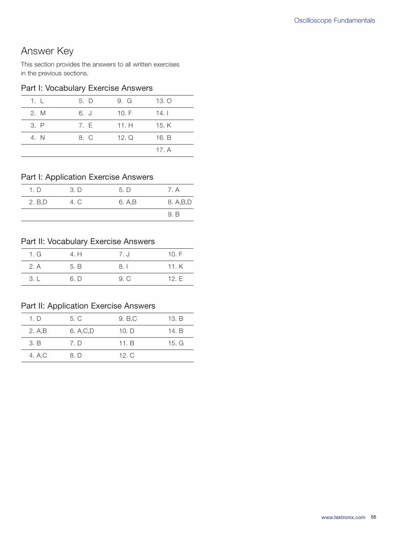
Oscilloscope Fundamentals
55www.tektronix.com
Answer KeyThis section provides the answers to all written exercises in the previous sections.
Part I: Vocabulary Exercise Answers
1. L 5. D 9. G 13. O
2. M 6. J 10. F 14. I
3. P 7. E 11. H 15. K
4. N 8. C 12. Q 16. B
17. A
Part I: Application Exercise Answers
1. D 3. D 5. D 7. A
2. B,D 4. C 6. A,B 8. A,B,D
9. B
Part II: Vocabulary Exercise Answers
1. G 4. H 7. J 10. F
2. A 5. B 8. I 11. K
3. L 6. D 9. C 12. E
Part II: Application Exercise Answers
1. D 5. C 9. B,C 13. B
2. A,B 6. A,C,D 10. D 14. B
3. B 7. D 11. B 15. G
4. A,C 8. D 12. C
03W-8605-4_edu.qxd 3/31/09 1:56 PM Page 55
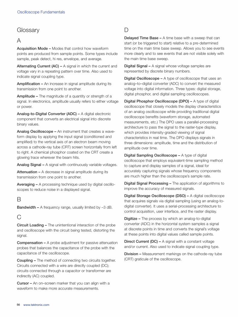
Oscilloscope Fundamentals
Glossary
AAcquisition Mode – Modes that control how waveformpoints are produced from sample points. Some types includesample, peak detect, hi res, envelope, and average.
Alternating Current (AC) – A signal in which the current andvoltage vary in a repeating pattern over time. Also used toindicate signal coupling type.
Amplification – An increase in signal amplitude during itstransmission from one point to another.
Amplitude – The magnitude of a quantity or strength of asignal. In electronics, amplitude usually refers to either voltageor power.
Analog-to-Digital Converter (ADC) – A digital electroniccomponent that converts an electrical signal into discretebinary values.
Analog Oscilloscope – An instrument that creates a wave-form display by applying the input signal (conditioned andamplified) to the vertical axis of an electron beam movingacross a cathode-ray tube (CRT) screen horizontally from leftto right. A chemical phosphor coated on the CRT create aglowing trace wherever the beam hits.
Analog Signal – A signal with continuously variable voltages.
Attenuation – A decrease in signal amplitude during itstransmission from one point to another.
Averaging – A processing technique used by digital oscillo-scopes to reduce noise in a displayed signal.
BBandwidth – A frequency range, usually limited by –3 dB.
CCircuit Loading – The unintentional interaction of the probeand oscilloscope with the circuit being tested, distorting thesignal.
Compensation – A probe adjustment for passive attenuationprobes that balances the capacitance of the probe with thecapacitance of the oscilloscope.
Coupling – The method of connecting two circuits together.Circuits connected with a wire are directly coupled (DC); circuits connected through a capacitor or transformer areindirectly (AC) coupled.
Cursor – An on–screen marker that you can align with awaveform to make more accurate measurements.
DDelayed Time Base – A time base with a sweep that canstart (or be triggered to start) relative to a pre-determinedtime on the main time base sweep. Allows you to see eventsmore clearly and to see events that are not visible solely withthe main time base sweep.
Digital Signal – A signal whose voltage samples are represented by discrete binary numbers.
Digital Oscilloscope – A type of oscilloscope that uses ananalog–to–digital converter (ADC) to convert the measuredvoltage into digital information. Three types: digital storage,digital phosphor, and digital sampling oscilloscopes.
Digital Phosphor Oscilloscope (DPO) – A type of digitaloscilloscope that closely models the display characteristics of an analog oscilloscope while providing traditional digitaloscilloscope benefits (waveform storage, automated measurements, etc.) The DPO uses a parallel-processingarchitecture to pass the signal to the raster-type display,which provides intensity-graded viewing of signal characteristics in real time. The DPO displays signals in three dimensions: amplitude, time and the distribution of amplitude over time.
Digital Sampling Oscilloscope – A type of digital oscilloscope that employs equivalent-time sampling methodto capture and display samples of a signal, ideal for accurately capturing signals whose frequency componentsare much higher than the oscilloscope’s sample rate.
Digital Signal Processing – The application of algorithms toimprove the accuracy of measured signals.
Digital Storage Oscilloscope (DSO) – A digital oscilloscopethat acquires signals via digital sampling (using an analog-to-digital converter). It uses a serial-processing architecture tocontrol acquisition, user interface, and the raster display.
Digitize – The process by which an analog-to-digital converter (ADC) in the horizontal system samples a signal at discrete points in time and converts the signal’s voltage at these points into digital values called sample points.
Direct Current (DC) – A signal with a constant voltageand/or current. Also used to indicate signal coupling type.
Division – Measurement markings on the cathode-ray tube(CRT) graticule of the oscilloscope.
56 www.tektronix.com
03W-8605-4_edu.qxd 3/31/09 1:56 PM Page 56
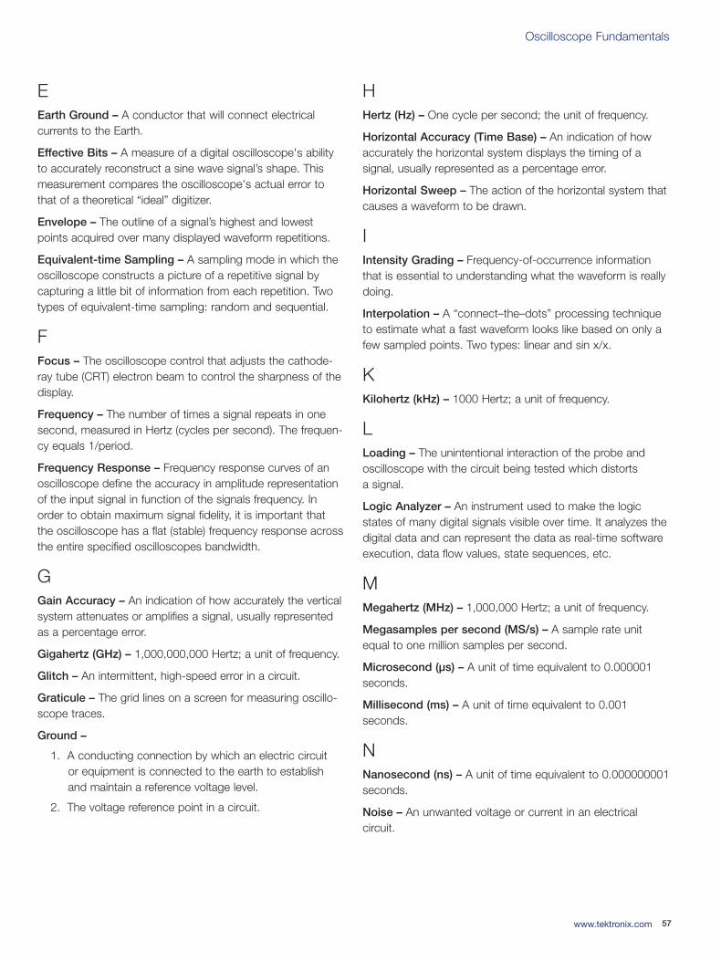
Oscilloscope Fundamentals
57www.tektronix.com
EEarth Ground – A conductor that will connect electrical currents to the Earth.
Effective Bits – A measure of a digital oscilloscope's abilityto accurately reconstruct a sine wave signal’s shape. Thismeasurement compares the oscilloscope's actual error tothat of a theoretical “ideal” digitizer.
Envelope – The outline of a signal’s highest and lowestpoints acquired over many displayed waveform repetitions.
Equivalent-time Sampling – A sampling mode in which theoscilloscope constructs a picture of a repetitive signal bycapturing a little bit of information from each repetition. Twotypes of equivalent-time sampling: random and sequential.
FFocus – The oscilloscope control that adjusts the cathode-ray tube (CRT) electron beam to control the sharpness of thedisplay.
Frequency – The number of times a signal repeats in onesecond, measured in Hertz (cycles per second). The frequen-cy equals 1/period.
Frequency Response – Frequency response curves of anoscilloscope define the accuracy in amplitude representationof the input signal in function of the signals frequency. Inorder to obtain maximum signal fidelity, it is important that the oscilloscope has a flat (stable) frequency response acrossthe entire specified oscilloscopes bandwidth.
GGain Accuracy – An indication of how accurately the verticalsystem attenuates or amplifies a signal, usually representedas a percentage error.
Gigahertz (GHz) – 1,000,000,000 Hertz; a unit of frequency.
Glitch – An intermittent, high-speed error in a circuit.
Graticule – The grid lines on a screen for measuring oscillo-scope traces.
Ground –
1. A conducting connection by which an electric circuit or equipment is connected to the earth to establish and maintain a reference voltage level.
2. The voltage reference point in a circuit.
HHertz (Hz) – One cycle per second; the unit of frequency.
Horizontal Accuracy (Time Base) – An indication of howaccurately the horizontal system displays the timing of a signal, usually represented as a percentage error.
Horizontal Sweep – The action of the horizontal system thatcauses a waveform to be drawn.
IIntensity Grading – Frequency-of-occurrence informationthat is essential to understanding what the waveform is reallydoing.
Interpolation – A “connect–the–dots” processing techniqueto estimate what a fast waveform looks like based on only afew sampled points. Two types: linear and sin x/x.
KKilohertz (kHz) – 1000 Hertz; a unit of frequency.
LLoading – The unintentional interaction of the probe andoscilloscope with the circuit being tested which distorts a signal.
Logic Analyzer – An instrument used to make the logicstates of many digital signals visible over time. It analyzes thedigital data and can represent the data as real-time softwareexecution, data flow values, state sequences, etc.
MMegahertz (MHz) – 1,000,000 Hertz; a unit of frequency.
Megasamples per second (MS/s) – A sample rate unitequal to one million samples per second.
Microsecond (µs) – A unit of time equivalent to 0.000001seconds.
Millisecond (ms) – A unit of time equivalent to 0.001 seconds.
NNanosecond (ns) – A unit of time equivalent to 0.000000001seconds.
Noise – An unwanted voltage or current in an electrical circuit.
03W-8605-4_edu.qxd 3/31/09 1:56 PM Page 57
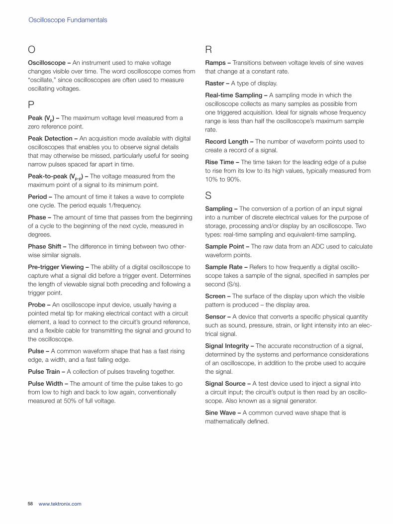
Oscilloscope Fundamentals
OOscilloscope – An instrument used to make voltagechanges visible over time. The word oscilloscope comes from“oscillate,” since oscilloscopes are often used to measureoscillating voltages.
PPeak (Vp) – The maximum voltage level measured from azero reference point.
Peak Detection – An acquisition mode available with digitaloscilloscopes that enables you to observe signal details that may otherwise be missed, particularly useful for seeingnarrow pulses spaced far apart in time.
Peak-to-peak (Vp-p) – The voltage measured from the maximum point of a signal to its minimum point.
Period – The amount of time it takes a wave to completeone cycle. The period equals 1/frequency.
Phase – The amount of time that passes from the beginningof a cycle to the beginning of the next cycle, measured indegrees.
Phase Shift – The difference in timing between two other-wise similar signals.
Pre-trigger Viewing – The ability of a digital oscilloscope tocapture what a signal did before a trigger event. Determinesthe length of viewable signal both preceding and following atrigger point.
Probe – An oscilloscope input device, usually having a pointed metal tip for making electrical contact with a circuitelement, a lead to connect to the circuit’s ground reference,and a flexible cable for transmitting the signal and ground tothe oscilloscope.
Pulse – A common waveform shape that has a fast risingedge, a width, and a fast falling edge.
Pulse Train – A collection of pulses traveling together.
Pulse Width – The amount of time the pulse takes to gofrom low to high and back to low again, conventionally measured at 50% of full voltage.
RRamps – Transitions between voltage levels of sine wavesthat change at a constant rate.
Raster – A type of display.
Real-time Sampling – A sampling mode in which the oscilloscope collects as many samples as possible from one triggered acquisition. Ideal for signals whose frequencyrange is less than half the oscilloscope’s maximum samplerate.
Record Length – The number of waveform points used tocreate a record of a signal.
Rise Time – The time taken for the leading edge of a pulseto rise from its low to its high values, typically measured from10% to 90%.
SSampling – The conversion of a portion of an input signalinto a number of discrete electrical values for the purpose ofstorage, processing and/or display by an oscilloscope. Twotypes: real-time sampling and equivalent-time sampling.
Sample Point – The raw data from an ADC used to calculatewaveform points.
Sample Rate – Refers to how frequently a digital oscillo-scope takes a sample of the signal, specified in samples persecond (S/s).
Screen – The surface of the display upon which the visiblepattern is produced – the display area.
Sensor – A device that converts a specific physical quantitysuch as sound, pressure, strain, or light intensity into an elec-trical signal.
Signal Integrity – The accurate reconstruction of a signal,determined by the systems and performance considerationsof an oscilloscope, in addition to the probe used to acquirethe signal.
Signal Source – A test device used to inject a signal into a circuit input; the circuit’s output is then read by an oscillo-scope. Also known as a signal generator.
Sine Wave – A common curved wave shape that is mathematically defined.
58 www.tektronix.com
03W-8605-4_edu.qxd 3/31/09 1:56 PM Page 58
Oscilloscope Fundamentals
59www.tektronix.com
Single Shot – A signal measured by an oscilloscope thatonly occurs once (also called a transient event).
Single Sweep – A trigger mode to display one triggeredscreen of a signal and then stop.
Slope – On a graph or an oscilloscope screen, the ratio of avertical distance to a horizontal distance. A positive slopeincreases from left to right, while a negative slope decreasesfrom left to right.
Square Wave – A common wave shape consisting of repeating square pulses.
Sweep – One horizontal pass of an oscilloscope’s electronbeam from left to right across the CRT screen.
Sweep Speed – Same as the time base.
TTime Base – Oscilloscope circuitry that controls the timing of the sweep. The time base is set by the seconds/divisioncontrol.
Trace – The visible shapes drawn on a CRT by the move-ment of the electron beam.
Transient – A signal measured by an oscilloscope that onlyoccurs once (also called a single–shot event).
Trigger – The circuit that references a horizontal sweep on an oscilloscope.
Trigger Holdoff – A control that allows you to adjust the period of time after a valid trigger during which the oscilloscope cannot trigger.
Trigger Level – The voltage level that a trigger source signalmust reach before the trigger circuit initiates a sweep.
Trigger Mode – A mode that determines whether or not theoscilloscope draws a waveform if it does not detect a trigger.Common trigger modes include normal and auto.
Trigger Slope – The slope that a trigger source signal mustreach before the trigger circuit initiates a sweep.
VVertical Resolution (Analog-to-Digital Converter) –An indication of how precisely an analog-to-digital converter(ADC) in a digital oscilloscope can convert input voltages into digital values, measured in bits. Calculation techniques,such as hi res acquisition mode, can improve the effectiveresolution.
Vertical Sensitivity – An indication of how much the vertical amplifier can amplify a weak signal – usually measured in millivolts (mV) per division.
Volt – The unit of electric potential difference.
Voltage – The difference in electric potential, expressed involts, between two points.
WWave – The generic term for a pattern that repeats over time. Common types include: sine, square, rectangular, saw-tooth, triangle, step, pulse, periodic, non-periodic, synchronous, asynchronous.
Waveform – A graphic representation of a voltage varyingover time.
Waveform Capture Rate – Refers to how quickly an oscilloscope acquires waveforms, expressed as waveformsper second (wfms/s).
Waveform Point – A digital value that represents the voltageof a signal at a specific point in time. Waveform points arecalculated from sample points and stored in memory.
Writing Speed – The ability of an analog oscilloscope to provide a visible trace of the movement of a signal from one point to another. This ability is restrictive for low-repetitionsignals that have fast-moving details, such as digital logic signals.
ZZ Axis – The display attribute on an oscilloscope that showsbrightness variations as the trace is formed.
03W-8605-4_edu.qxd 3/31/09 1:56 PM Page 59
For Further InformationTektronix maintains a comprehensive, constantly expandingcollection of application notes, technical briefs and otherresources to help engineers working on the cutting edge oftechnology. Please visit www.tektronix.com
Copyright © 2009, Tektronix. All rights reserved. Tektronix products are covered by U.S. and foreign patents, issued and pending. Information in this publicationsupersedes that in all previously published material. Specification and pricechange privileges reserved. TEKTRONIX and TEK are registered trademarks of Tektronix, Inc. All other trade names referenced are the service marks, trademarks or registered trademarks of their respective companies. 03/09 JS/WWW 03W-8605-4
Contact Tektronix:ASEAN / Australasia (65) 6356 3900
Austria +41 52 675 3777
Balkans, Israel, South Africa and other ISE Countries +41 52 675 3777
Belgium 07 81 60166
Brazil +55 (11) 40669400
Canada 1 (800) 661-5625
Central East Europe, Ukraine and the Baltics +41 52 675 3777
Central Europe & Greece +41 52 675 3777
Denmark +45 80 88 1401
Finland +41 52 675 3777
France +33 (0) 1 69 86 81 81
Germany +49 (221) 94 77 400
Hong Kong (852) 2585-6688
India (91) 80-42922600
Italy +39 (02) 25086 1
Japan 81 (3) 6714-3010
Luxembourg +44 (0) 1344 392400
Mexico, Central/South America & Caribbean 52 (55) 54247900
Middle East, Asia and North Africa +41 52 675 3777
The Netherlands 090 02 021797
Norway 800 16098
People’s Republic of China 86 (10) 6235 1230
Poland +41 52 675 3777
Portugal 80 08 12370
Republic of Korea 82 (2) 6917-5000
Russia & CIS +7 (495) 7484900
South Africa +27 11 206 8360
Spain (+34) 901 988 054
Sweden 020 08 80371
Switzerland +41 52 675 3777
Taiwan 886 (2) 2722-9622
United Kingdom & Ireland +44 (0) 1344 392400
USA 1 (800) 426-2200
For other areas contact Tektronix, Inc. at: 1 (503) 627-7111
Updated 30 October 2008
03W-8605-4_edu.qxd 3/31/09 1:56 PM Page 60