Oscillatory Waves in Inhomogeneous Neural Media

P. C. Bressloff,1 S. E. Folias,1 A. Prat,2 and Y.-X. Li2

1Department of Mathematics, University of Utah, Salt Lake City, Utah 84112, USA2Departments of Mathematics and Zoology, University of British Columbia, Vancouver, BC, Canada V6T 1Z2

(Received 14 May 2003; revised manuscript received 25 August 2003; published 23 October 2003)

In this Letter we show that an inhomogeneous input can induce wave propagation failure in anexcitatory neural network due to the pinning of a stationary front or pulse solution. A subsequentreduction in the strength of the input can lead to a Hopf instability of the stationary solution resulting inbreatherlike oscillatory waves.

DOI: 10.1103/PhysRevLett.91.178101 PACS numbers: 87.19.La, 05.45.Xt, 82.40.Bj

A number of theoretical studies have established theoccurrence of traveling fronts [1,2] and traveling pulses[3–5] in one-dimensional excitatory neural networksmodeled in terms of evolution equations of the form

�@u�x; t�

@t� u�x; t� �

Z 1

�1w�x j x0�f�u�x0; t��dx0

� v�x; t� � I�x�;1

"

@v�x; t�

@t� v�x; t� � u�x; t�;

(1)

where u�x; t� is a neural field that represents the localactivity of a population of excitatory neurons at positionx 2 R, I�x� is an external input, � is a synaptic timeconstant (assuming first-order or exponential synapses),f�u� denotes an output firing rate function, andw�x j x0� isthe strength of connections from neurons at x0 to neuronsat x. The neural field v�x; t� represents some form ofnegative feedback recovery mechanism such as spikefrequency adaptation or synaptic depression, with ; "determining the relative strength and rate of feedback.(One can also incorporate higher-order synaptic and den-dritic processes by replacing �@u=@t� u with a moregeneral linear differential operator L̂Lu.) It has been estab-lished [5] that there is a direct link between the abovemodel and experimental studies of wave propagation incortical slices where synaptic inhibition is pharmacologi-cally blocked [6–8]. Since there is strong vertical cou-pling between cortical layers, it is possible to treat a thincortical slice as an effective one-dimensional medium.Analysis of the model provides valuable informationregarding how the speed of a traveling wave, which isrelatively straightforward to measure experimentally,depends on various features of the underlying corticalcircuitry.

One of the basic assumptions in the analysis of travel-ing wave solutions of Eq. (1) is that the system is spatiallyhomogeneous, that is, the external input I�x� is indepen-dent of x and the synaptic weights depend only on thedistance between presynaptic and postsynaptic cells,w�x j x0� � w�x� x0� with w a monotonically decreasingfunction of cortical separation. It can then be established

that waves are in the form of traveling fronts in theabsence of any feedback, whereas traveling pulses tendto occur when there is significant feedback [5]. However,the cortex is more realistically modeled as an inhomoge-neous medium. For example, inhomogeneities in the syn-aptic weight distribution w are likely to arise due to thepatchy nature of long-range horizontal connections insuperficial layers of cortex [9]. Another important sourceof inhomogeneity arises from external inputs induced bysensory stimuli, which may be modeled in terms of anonuniform input I�x�. In this Letter we show that forappropriate choices of input inhomogeneity, wave propa-gation failure can occur due to the pinning of a stationaryfront or pulse solution. More significantly, we findthat these stationary solutions can undergo a Hopf insta-bility at a critical input amplitude, below which an oscil-latory back-and-forth pattern of wave propagation or‘‘breather’’ is observed. Our analysis predicts that theHopf frequency depends on the relative strength andrate of feedback, but is independent of the details of theweight distribution. We also show numerically how asecondary instability leads to the generation of travelingwaves. Analogous breatherlike solutions have been foundin inhomogeneous reaction-diffusion systems [10,11] andin numerical simulations of a realistic model of fertiliza-tion calcium waves [12].

First, let us consider traveling front solutions of Eq. (1)in the case of zero input I�x� � 0 and homogeneousweights w�x j x0� � w�x� x0�. For mathematical conve-nience, we take w�x� � �2d��1e�jxj=d with

R1�1w�y�dy �

1. The time and length scales are fixed by setting� � d � 1; typical values for these parameters are � �10 msec and d � 1 mm. As a further simplification, letf�u� � �u� �� where is the Heaviside step functionand � is a threshold. We then seek a traveling frontsolution of the form u�x; t� � U���, � � x� ct, c > 0,such thatU�0� � �,U���< � for � > 0 andU��� > � for� < 0. The center of the wave is arbitrary due to thetranslation symmetry of the homogeneous system.Eliminating the variable V��� � v�x� ct� by differenti-ating Eq. (1) twice with respect to �, leads to the second-order differential equation

P H Y S I C A L R E V I E W L E T T E R S week ending24 OCTOBER 2003VOLUME 91, NUMBER 17

178101-1 0031-9007=03=91(17)=178101(4)$20.00 2003 The American Physical Society 178101-1

�c2U00��� � c1� "�U0��� � "1� �U��� � �cw��� � "W���; (2)

where 0 denotes differentiation with respect to � andW��� �

R1� w�y�dy. The boundary conditions are U�0� �

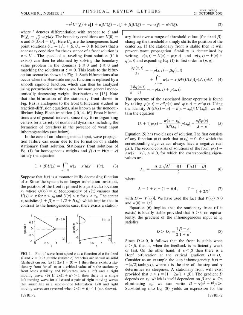
� andU��1� � U�. HereU� are the homogeneous fixedpoint solutions U� � 1=1� ;U� � 0. It follows that anecessary condition for the existence of a front solution is� < U�. The speed of a traveling front solution (if itexists) can then be obtained by solving the boundaryvalue problem in the domains � 0 and � � 0 andmatching the solutions at � � 0. This leads to the bifur-cation scenarios shown in Fig. 1. Such bifurcations alsooccur when the Heaviside output function is replaced by asmooth sigmoid function, which can then be analyzedusing perturbation methods, and for more general mono-tonically decreasing weight distributions w [13]. Notethat the bifurcation of the stationary front shown inFig. 1(a) is analogous to the front bifurcation studied inreaction-diffusion equations, also known as the nonequi-librium Ising-Bloch transition [10,14–16]. Front bifurca-tions are of general interest, since they form organizingcenters for a variety of nontrivial dynamics including theformation of breathers in the presence of weak inputinhomogeneities (see below).

In the case of an inhomogeneous input, wave propaga-tion failure can occur due to the formation of a stablestationary front solution. Stationary front solutions ofEq. (1) for homogeneous weights and f�u� � �u� ��satisfy the equation

�1� �U�x� �Z x0

�1w�x� x0�dx0 � I�x�: (3)

Suppose that I�x� is a monotonically decreasing functionof x. Since the system is no longer translation invariant,the position of the front is pinned to a particular locationx0 where U�x0� � �. Monotonicity of I�x� ensures thatU�x� > � for x < x0 and U�x�< � for x > x0. The centerx0 satisfies �1� �� � 1=2� I�x0�, which implies that incontrast to the homogeneous case, there exists a station-

ary front over a range of threshold values (for fixed );changing the threshold � simply shifts the position of thecenter x0. If the stationary front is stable then it willprevent wave propagation. Stability is determined bywriting u�x; t� � U�x� � p�x; t� and v�x; t� � V�x� �q�x; t� and expanding Eq. (1) to first order in �p; q�:

@p�x; t�

@t� �p�x; t� � q�x; t�

�Z 1

�1w�x� x0�H0�U�x0��p�x0; t�dx0;

1

"

@q�x; t�

@t� �q�x; t� � p�x; t�:

(4)

The spectrum of the associated linear operator is foundby taking p�x; t� � e�tp�x� and q�x; t� � e�tq�x�. Usingthe identity H0�U�x� � �� � ��x� x0�=jU

0�x0�j, we ob-tain the equation

��� 1�p�x� �w�x� x0�

jU0�x0�jp�x0� �

"p�x�

�� ": (5)

Equation (5) has two classes of solution. The first consistsof any function p�x� such that p�x0� � 0, for which thecorresponding eigenvalues always have a negative realpart. The second consists of solutions of the form p�x� �Aw�x� x0�, A � 0, for which the corresponding eigen-values are

�� ���

��������������������������������������������������

2 � 4�1� ��"�1� �p

2; (6)

where

� 1� "� �1� ��; � �1

1� 2D; (7)

with D � jI0�x0�j. We have used the fact that I0�x0� 0

and w�0� � 1=2.Equation (6) implies that the stationary front (if it

exists) is locally stable provided that > 0 or, equiva-lently, the gradient of the inhomogeneous input at x0satisfies

D > Dc �1

2

� "

1� ": (8)

Since D � 0, it follows that the front is stable when" > , that is, when the feedback is sufficiently weakor fast. On the other hand, if " < then there is aHopf bifurcation at the critical gradient D � Dc.Consider as an example the step inhomogeneity I�x� ���s=2� tanh�#x�, where s is the size of the step and #determines its steepness. A stationary front will existprovided that s > �ss � j1� 2��1� �j. The gradient Ddepends on x0, which is itself dependent on and �. Oneliminating x0, we can write D � #�s2 � �ss2�=2s.Substituting into Eq. (8) yields an expression for the

0 0.5 1 1.5-1

-0.5

0

0.5

1

0 0.5 1 1.5

-2

-1

0

1

speed c

ε

β = 1.0

ε

β = 1.5

(a) (b)

speed c

FIG. 1. Plot of wave front speed c as a function of " for fixed and � � 0:25. Stable (unstable) branches are shown as solid(dashed) curves. (a) If 2��1� � � 1 then there exists a sta-tionary front for all "; at a critical value of " the stationaryfront loses stability and bifurcates into a left and a rightmoving wave. (b) If 2��1� � > 1 then there is a singleleft-moving wave for all " and a pair of right-moving wavesthat annihilate in a saddle-node bifurcation. Left and rightmoving waves are reversed when 2��1� �< 1 (not shown).

P H Y S I C A L R E V I E W L E T T E R S week ending24 OCTOBER 2003VOLUME 91, NUMBER 17

178101-2 178101-2

critical value of s that determines the Hopf bifurcationpoints:

sc �1

2#

�� "

1� "�

��������������������������������������� "

1� "

�2

�4�ss2#2

s

: (9)

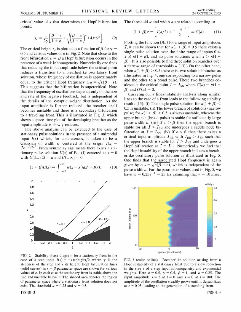
The critical height sc is plotted as a function of for # �0:5 and various values of " in Fig. 2. Note that close to thefront bifurcation " � a Hopf bifurcation occurs in thepresence of a weak inhomogeneity. Numerically one findsthat reducing the input amplitude below the critical pointinduces a transition to a breatherlike oscillatory frontsolution, whose frequency of oscillation is approximately

equal to the critical Hopf frequency !H ��������������������

"�� "�p

.This suggests that the bifurcation is supercritical. Notethat the frequency of oscillations depends only on the sizeand rate of the negative feedback, but is independent ofthe details of the synaptic weight distribution. As theinput amplitude is further reduced, the breather itselfbecomes unstable and there is a secondary bifurcationto a traveling front. This is illustrated in Fig. 3, whichshows a space-time plot of the developing breather as theinput amplitude is slowly reduced.

The above analysis can be extended to the case ofstationary pulse solutions in the presence of a unimodalinput I�x� which, for concreteness, is taken to be aGaussian of width % centered at the origin I�x� �Ie�x

2=2%2

. From symmetry arguments there exists a sta-tionary pulse solution U�x� of Eq. (1) centered at x � 0

with U��a=2� � � and U��1� � 0:

�1� �U�x� �Z a=2

�a=2w�x� x0�dx0 � I�x�: (10)

The threshold � and width a are related according to

�1� �� �

�

I�a=2� �1� e�a

2

� G�a�: (11)

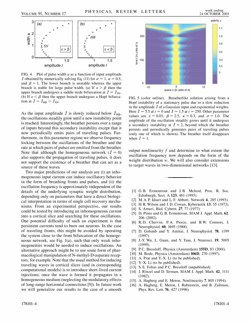
Plotting the functionG�a� for a range of input amplitudesI , it can be shown that for ��1� �< 0:5 there exists asingle pulse solution over the finite range of inputs 0 I ��1� �, and no pulse solutions when I > ��1��. (It is also possible to find three solution branches overa narrow range of thresholds � [13].) On the other hand,when ��1� � > 0:5 there exist two solution branches asillustrated in Fig. 4, one corresponding to a narrow pulseand the other to a broad pulse. These two branches co-alesce at the critical point I � ISN where G�a� � ��1�� and G0�a� � 0.

Carrying out a linear stability analysis along similarlines to the case of a front leads to the following stabilityresults [13]: (i) The single pulse solution for ��1� �<0:5 is unstable. (ii) The lower branch of solutions (narrowpulse) for ��1� � > 0:5 is always unstable, whereas theupper branch (broad pulse) is stable for sufficiently largepulse width a. (iii) If " > then the upper branch isstable for all I > ISN and undergoes a saddle node bi-furcation at I � ISN. (iv) If " < then there exists acritical input amplitude IHB with IHB > ISN such thatthe upper branch is stable for I > IHB and undergoes aHopf bifurcation at I � IHB. Numerically we find thatthe Hopf instability of the upper branch induces a breath-erlike oscillatory pulse solution as illustrated in Fig. 5.One finds that the associated Hopf frequency is againgiven by !H �

�������������������

"�� "�p

, which is independent of thepulse width a. For the parameter values used in Fig. 5, wehave ! � 0:25��1 � 25 Hz assuming that � � 10 msec.

FIG. 2. Stability phase diagram for a stationary front in thecase of a step input I�x� � �s tanh�#x�=2 where # is thesteepness of the step and s its height. Hopf bifurcation lines(solid curves) in s� parameter space are shown for variousvalues of ". In each case the stationary front is stable above theline and unstable below it. The shaded area denotes the regionof parameter space where a stationary front solution does notexist. The threshold � � 0:25 and # � 0:5.

FIG. 3 (color online). Breatherlike solution arising from aHopf instability of a stationary front due to a slow reductionin the size s of a step input inhomogeneity and exponentialweights. Here " � 0:5, # � 0:5, � 1, and � � 0:25. Theinput amplitude s � 2 at t � 0 and s � 0 at t � 180. Theamplitude of the oscillation steadily grows until it destabilizesat s � 0:05, leading to the generation of a traveling front.

P H Y S I C A L R E V I E W L E T T E R S week ending24 OCTOBER 2003VOLUME 91, NUMBER 17

178101-3 178101-3

As the input amplitude I is slowly reduced below IHB,the oscillations steadily grow until a new instability pointis reached. Interestingly, the breather persists over a rangeof inputs beyond this secondary instability except that itnow periodically emits pairs of traveling pulses. Fur-thermore, in this parameter regime we observe frequencylocking between the oscillations of the breather and therate at which pairs of pulses are emitted from the breather.Note that although the homogeneous network (I � 0)also supports the propagation of traveling pulses, it doesnot support the existence of a breather that can act as asource of these waves.

Two major predictions of our analysis are (i) an inho-mogeneous input current can induce oscillatory behaviorin the form of breathing fronts and pulses, and (ii) theoscillation frequency is approximately independent of thedetails of the underlying synaptic weight distribution,depending only on parameters that have a direct biologi-cal interpretation in terms of single cell recovery mecha-nisms. From an experimental perspective, our resultscould be tested by introducing an inhomogeneous currentinto a cortical slice and searching for these oscillations.One potential difficulty of such an experiment is thatpersistent currents tend to burn out neurons. In the caseof traveling fronts, this might be avoided by operatingthe system close to the front bifurcation of the homoge-neous network, see Fig. 1(a), such that only weak inho-mogeneities would be needed to induce oscillations. Analternative approach might be to use some form of phar-macological manipulation of N-methyl-D-asparate recep-tors, for example. Note that the usual method for inducingtraveling waves in cortical slices (and in correspondingcomputational models) is to introduce short-lived currentinjections; once the wave is formed it propagates in ahomogeneous medium (neglecting the modulatory effectsof long-range horizontal connections [9]). In future workwe will generalize our results to the case of a smooth

output nonlinearity f and determine to what extent theoscillation frequency now depends on the form of theweight distribution w. We will also consider extensionsto target waves in two-dimensional networks [13].

[1] G. B. Ermentrout and J. B. Mcleod, Proc. R. Soc.Edinburgh, Sect. A 123, 461 (1993).

[2] M. A. P. Idiart and L. F. Abbott, Network 4, 285 (1993).[3] H. R. Wilson and J. D. Cowan, Kybernetik 13, 55 (1973).[4] S. Amari, Biol. Cybern. 27, 77 (1977).[5] D. Pinto and G. B. Ermentrout, SIAM J. Appl. Math. 62,

206 (2002).[6] R. D. Chervin, P. A. Pierce, and B.W. Connors, J.

Neurophysiol. 60, 1695 (1988).[7] D. Golomb and Y. Amitai, J. Neurophysiol. 78, 1199

(1997).[8] J.-Y. Wu, L. Guan, and Y. Tsau, J. Neurosci. 19, 5005

(1999).[9] P. C. Bressloff, Physica (Amsterdam) 155D, 83 (2001).

[10] M. Bode, Physica (Amsterdam) 106D, 270 (1997).[11] A. Prat and Y.-X. Li (to be published).[12] Y.-X. Li (to be published).[13] S. E. Folias and P. C. Bressloff (unpublished).[14] J. Rinzel and D. Terman, SIAM J. Appl. Math. 42, 1111

(1982).[15] A. Hagberg and E. Meron, Nonlinearity 7, 805 (1994).[16] A. Hagberg, E. Meron, I. Rubinstein, and B. Zaltman,

Phys. Rev. Lett. 76, 427 (1996).

FIG. 5 (color online). Breatherlike solution arising from aHopf instability of a stationary pulse due to a slow reductionin the amplitude I of a Gaussian input and exponential weights.Here I � 5:5 at t � 0 and I � 1:5 at t � 250. Other parametervalues are " � 0:03, � 2:5, � � 0:3, and % � 1:0. Theamplitude of the oscillation steadily grows until it undergoesa secondary instability at I � 2, beyond which the breatherpersists and periodically generates pairs of traveling pulses(only one of which is shown). The breather itself disappearswhen I � 1.

1 1.50

1

2

3

amplitude I

wid

th a

SN

amplitude I

HB

(a)

ε > β

1 1.5

(b)

ε < β

FIG. 4. Plot of pulse width a as a function of input amplitudeI obtained by numerically solving Eq. (11) for % � 1, � � 0:5,and � 1. The lower branch is unstable whereas the upperbranch is stable for large pulse width. (a) If " > then theupper branch undergoes a saddle-node bifurcation at I � ISN.(b) If " < then the upper branch undergoes a Hopf bifurca-tion at I � IHB > ISN.

P H Y S I C A L R E V I E W L E T T E R S week ending24 OCTOBER 2003VOLUME 91, NUMBER 17

178101-4 178101-4