ORTHOGONAL SIMPLE COMPONENT ANALYSISstats- · ORTHOGONAL SIMPLE COMPONENT ANALYSIS By Karim Anaya-Izquierdo, ... Again, exact zeros and simple averages appear natu-rally

Submitted to the Annals of Applied Statistics

ORTHOGONAL SIMPLE COMPONENT ANALYSIS

By Karim Anaya-Izquierdo, Frank Critchley and Karen Vines

The Open University

A new methodology to aid interpretation of a principal compo-nent analysis is presented. While preserving orthogonality, each eigen-vector is replaced by a vector, close to it in angle terms, whose entriesare small integers. We call such vectors simple. The approach is ex-ploratory, a range of sets of pairwise orthogonal simple componentsbeing systematically obtained, from which the user may choose. Ex-amples and simulations show that this approach effectively combinessimplicity, retention of optimality and computational efficiency. Fur-ther, when the population eigenvectors have simple structure, thiscan be recovered using only the information from the sample. Themethodology can also be used to simplify a given subset of com-ponents. An efficient algorithm for the computationally challengingproblem of producing orthogonal components is provided.

1. Introduction. Principal components are optimal linear combinations of a set of variableswith coefficients given by the eigenvectors of the covariance or correlation matrix ((8) chapters 2and 3). To be useful in practice, such components often need interpretation in the context of thedata studied. Unfortunately, the optimality of these principal components does not ensure theyhave a simple interpretation. They may possess optimal theoretical properties, but be of limitedpractical interest. This motivates replacing them by simpler, more interpretable, components, atthe expense of a certain degree of optimality.

In a broad sense, simplicity means the appearance of nice structures in the loadings matrixQ = (q1|...|qk). Often, the scientist in charge of the study, would like to see clear-cut patterns inQ which help him or her to better understand the meaning of the components q>r x (r = 1, ..., k)which it generates. Examples of nice structures include sparseness, the presence of simple weightedaverages, contrasts and groups of variables. But simplicity inevitably implies loss of optimality,and it is the scientist in charge of the study who needs to calibrate the trade-off between simplicityand optimality.

The oldest approach to simplifying principal components is rotation (see (8), chapter 11 foran excellent review). Assuming normality, (12) recently proposed a penalised profile likelihoodmethod, using varimax as the penalty function, which favours rotation of ill-defined components(those whose eigenvalues are close). In general, rotation methods lead to orthogonal simplifiedcomponents defining new coordinate axes on which the data can be displayed, while total vari-ance is preserved. However, the loadings involved are usually real numbers, which means thatinterpretation can still be difficult.

Another approach to simplification is to target sparsity. The presence of many zeros in Q canbe useful for interpretation, for example when dealing with many variables. See, for example,(2), (3), (5), (11) and the references therein. One class of methods which targets sparseness isthat based on the Least Absolute Shrinkage Selection Operator (LASSO). See, for example, (9)(15), (18), and (20). Although most of these methods lead to orthogonal simplified components,

AMS 2000 subject classifications: Primary 62H25Keywords and phrases: simplified principal components, orthogonal integer loadings

1imsart-aoas ver. 2007/12/10 file: spca_final.tex date: August 7, 2008

2 ANAYA-IZQUIERDO ET AL.

combined with the presence of exact zero loadings, the remaining loadings are still real numbers,impeding interpretation.

A more explicitly modelling approach to simplification has recently been suggested by (14).Intrinsically restricted to principal component analysis of a correlation matrix, it assumes a par-ticular form of that matrix inducing a pattern in its eigenstructure in which groups and contrastsof variables are forced to appear. For example, when all variables are positively correlated, thefirst eigenvector is always close to the average of the variables and consequently the remainingeigenvectors are basically contrasts. The loadings obtained are all proportional to integers, aidinginterpretation. However, the components obtained need not be orthogonal.

(6), (16) and (19) suggest similar methods of simplification, in the sense that all three giveorthogonal components with loading vectors proportional to integers. Hausman’s method onlyallows the loadings to take the values −1, 0 or 1 and therefore is not always able to find acomplete set of orthogonal vectors. In contrast, Vines’ method produces loading vectors that areproportional to integers via a sequence of pairwise ‘simplicity-preserving’ transformations whichensure that orthogonality is maintained. However, although always proportional to integers, thesize of the integers is not bounded and may at times be very large. A fuller discussion of themethod, and its properties, can be found in (16).

The methodology we introduce in this paper produces the same clear structure as (19) for adata set with four different measurements of an index of resistance to flow in blood-vessels (17),as shown in Table 1:

Variable q1 z1 q2 z2 q3 z3 q4 z4

Right Doppler 0.42 1 −0.32 −1 −0.58 −1 −0.62 −1Left Doppler 0.43 1 0.30 1 −0.55 −1 0.65 1Right CVI 0.55 1 −0.65 −1 0.43 1 0.30 1Left CVI 0.58 1 0.63 1 0.42 1 −0.31 −1

% variance 58 57 25.9 23.8 9.5 10.5 6.5 8.6Table 1

Principal component loadings for the resistance index data q1, . . . ,q4 and the corresponding simplified loadingvectors z1, . . . , z4

The simplified loadings are easier to understand than the continuous ones, so much so in fact thatit looks like we have uncovered nature’s design: a main effect, plus three orthogonal contrasts.The simplified components being orthogonal, the total variance is retained, being redistributedamong the components so as to enhance interpretability. In particular, there is just a little loss inthe variance explained by the first two components.

In this paper, we propose a methodology to obtain simple approximations to the vectors ofloadings of the principal components with the following characteristics:

1. Proportionality to vectors of small integers.2. Individual angle-closeness.3. Pairwise orthogonality.

As examples and simulations will show, we can obtain good approximations in the sense thatonly small integers are used, while retaining closeness to the original components and exactorthogonality. The rationale behind the choice of these three characteristics is as follows:

1. Integers aid interpretation, vectors proportional to small integers being typically easier tointerpret than vectors of real entries. Again, exact zeros and simple averages appear natu-rally.

imsart-aoas ver. 2007/12/10 file: spca_final.tex date: August 7, 2008

ORTHOGONAL SIMPLE PCA 3

2. By keeping each approximating vector close to its exact counterpart, we ensure that wedo not lose potentially meaningful individual eigenvectors and that overall optimality ismaximally retained.

3. Orthogonality also aids interpretation. Contrasts, simple relations between components andgroups of variables may all appear as a direct consequence of using orthogonality combinedwith integer coefficients. Again, total variance is preserved, while simple components nowdefine orthogonal axes, relative to which data can be plotted and interpreted.

However, interpretability is neither guaranteed nor amenable to precise mathematical formula-tion. This has two, key, methodological consequences. Whereas, as we will show by example, ourapproach can help in the vital step of interpretation, we do not expect any method to lead tointerpretable results in all cases. Again, rather than attempt to find a unique optimal simplifica-tion in any pre-defined sense, we follow an exploratory approach which systematically produces arange of sets of pairwise orthogonal simple components, each close to its parent, amongst whichthe user can choose. Factors that can guide this choice include: (a) interpretability, simplicityand accuracy, as above, (b) subject matter considerations, particular to the context of the dataset under analysis, and (c) suboptimality with respect to exact principal component analysis,including lower explanatory power in terms of the proportion of total variance, loss of focus onpotential scientific laws (near constant relationships between the variables) and correlation. Onlyprincipal component analysis itself can give orthogonal loadings and uncorrelated components.So, as we require our simple loading vectors to be orthogonal, our components will always showsome degree of correlation.

The space of all integer orthogonal matrices is huge, the combinatorial complexity growing bothwith the number of variables and the maximum size of integer allowed. However, the nature of ourmethod allows efficient exploration of this vast space without restriction to any of its particularsubsets, such as those determined by modelling assumptions. Although other approaches arepossible, such as the one described in (1), the methodology proposed here relies on the fact thatinterpretation is possible using only the matrix of loadings.

The plan of the paper is as follows. Section 2 describes our methodology, discussing the ideasinvolved in detail and illustrating them with the help of a running example. Section 3 discusses twoother examples. Section 4 presents a simulation study that shows the exact recovery properties ofour method, while Section 5 discusses some possible extensions and other issues. Technical andcomputational details are given in an appendix.

2. Approximating eigenvectors.

2.1. General setup. Throughout this paper, the set of all integers and real numbers will bedenoted by Z and R respectively, while Z(k) and R(k) denote the punctured product spacesZk\{(0, . . . , 0)>} and Rk\{(0, . . . , 0)>} respectively. For any u ∈ R(k), `(u) := {cu : c ∈ R}will be called the axis generated by u.

Let S be a given k × k sample covariance or correlation matrix for a set of k commensurablevariables. We assume S is nonsingular with k distinct eigenvalues, denoted λ1 > . . . > λk > 0. Theoverall sign of the unit-length eigenvector associated with each λi being intrinsically indeterminate,we denote either by qi. The eigenspace corresponding to each λi is then the axis αi = `(qi), eachof which we approximate by some other axis αi. For any axis α = `(u) approximated by α = `(u),the angle discrepancy

d(α, α) := arccos

(|u>u|‖u‖‖u‖

)



defines a distance between them. The choice of this discrepancy is partly motivated by the factthat it does not depend on the choice of the nonzero vectors u and u within their spans. Forreporting purposes, we use the accuracy measure defined by accu(α, α) := cos(d(α, α)) whichtakes values in [0, 1].

q1 q2 q3 q4 q5

Mechanics (Closed) 0.40 -0.65 0.62 0.15 -0.13Vectors (Closed) 0.43 -0.44 -0.71 -0.30 -0.18Algebra (Open) 0.50 0.13 -0.04 0.11 0.85Analysis (Open) 0.46 0.39 -0.14 0.67 -0.42

Statistics (Open) 0.40 0.47 0.31 -0.66 -0.23

% variance 63.6 14.8 8.9 7.8 4.9

Table 2Principal component loadings for the exams data.

To illustrate our methodology we use, as a running example, a data set consisting of the scoresachieved by 88 students in 5 tests, a combination of open- and closed-book exams (10). Table 2shows the unit length eigenvectors (rounded to 2 decimal places) of the sample correlation matrixfor this data set. Thus, the first principal component is a weighted average of all the differentsubject scores and the other principal components can be interpreted as contrasts. However, moredetailed interpretation of the principal components, particularly those other than the first, is noteasy.

This section is organised as follows. Sections 2.2 and 2.3 describe how to obtain approximationsto all the eigenvectors, while Section 2.4 shows how the approach can be adapted to situationsin which only a subset of eigenvectors are of interest. Section 2.5 introduces three variants of ourmethodology, and some of their important features. Finally, in Section 2.6, we discuss how toproceed in practice and interpret the exams data based on our systematic, exploratory analysis.

2.2. Description of the approximations. We only consider approximations α which are gen-erated by integer vectors.

Definition 1. An axis α is called simple if there exists z ∈ Z(k) such that α = `(z). Ifthe nonzero elements of z are coprime, then z is called an integer representation of α and theirmaximum absolute value is called the complexity of α, denoted here by compl(α).

We approximate the {αr}kr=1 one at a time. The order in which we do this matters, different

orders providing different approximations. Subsuming a permutation of (1, . . . , k), there is no lossof generality in describing our approximations {αr}k

r=1 for a single, fixed order. Here, we fit theaxes with larger variances first – that is, we work in increasing numerical order. Other possibilitiesare described in Section 2.5.

For each r ∈ {1, . . . , k}, we construct an appropriate set Mr of simple axes, within which wethen find the best approximation αr to αr. The orthogonality of our approximating eigenvectorsis guaranteed by the way we construct Mr at each step. In the approximation of the first axisthere is no orthogonality restriction, so we take M1 to be set of all simple axes in Rk. For theexams data, M1 is the set of all axes generated by vectors in Z(5). Thus an approximation to α1

could be the simple axis generated by z1 = (1, 1, 1, 1, 1)>.For 2 ≤ r ≤ k − 1, we take Mr to be the set of all simple axes which are orthogonal to

α1, . . . , αr−1. Let Or−1 be a matrix whose columns are integer vectors, orthogonal to α1, . . . , αr−1.



To ensure our approximating axes are simple, we use linear combinations of the columns of Or−1

with integer coefficients to generate Mr. It is always possible to find such a matrix Or−1 (seeAppendix A). For the exams data, if we have α1 = `((1, 1, 1, 1, 1)>), a suitable O1 is

O1 =

1 1 1 1−1 0 0 0

0 −1 0 00 0 −1 00 0 0 −1

.

Thus, for example, if we take y> = (−1, 0, 1, 1), then

z2 =1

hcf(|O1 y|) O1 y = (1, 1, 0,−1,−1)>

is a member of M2, where hcf(|z|) denotes the highest common factor of the nonzero absolutevalues of the elements of z (dividing by it ensures the corresponding values for z2 are coprime).

Geometrically, it is clear that the angle-closest axis to α which is orthogonal to α1, . . . , αr−1

is its projection onto the orthogonal complement of their span, restricting the maximum accu-racy achievable. For, if q⊥r is the orthogonal projection of the unit vector qr onto Mr, for anyapproximation α ∈Mr,

accu(αr, α) = accu(αr, `(q⊥r )) accu(`(q⊥r ), α)

= ‖q⊥r ‖ accu(`(q⊥r ), α)

so that accu(αr, α) ≤ ‖q⊥r ‖, equality holding if and only if α = `(q⊥r ) (which requires `(q⊥r ) to besimple). Thus, over Mr, not every possible accuracy is achievable for αr, although no such upperbound applies to accu(`(q⊥r ), α).

For the exams data with α1 = `((1, 1, 1, 1, 1)>), the projection of q2 onto the orthogonalcomplement of α1 is q⊥2 = (−0.63,−0.42, 0.15, 0.41, 0.49)> (to 2 decimal places). Since ‖q⊥2 ‖ =0.999, there is no approximation to α2 orthogonal to α1 which can achieve an accuracy biggerthan this. In particular, α2 = `((1, 1, 0,−1,−1)>) has an accuracy of 0.973 with respect to α2,while its accuracy with respect to `(q⊥2 ) is given by accu(α2, α2)/‖q⊥2 ‖ = 0.973/0.999 ≈ 0.974.Similar information for other axes is given in Table 3.

Any given angle θ ∈ (0, π/2) defines a ‘cone’ around αr inMr of fixed complexity N ∈ {1, 2, . . .}via

Cr(θ,N) := {α ∈Mr : accu(α, αr) ≥ cos(θ) , compl(α) = N}.If cos(θ) > ‖q⊥r ‖, then Cr(θ,N) is empty for all N , so we always take cos(θ) ≤ ‖q⊥r ‖. For given θ,we are interested in the nonempty cone with smallest complexity, namely C∗

r (θ) := Cr(θ, Nr(θ)),where

(2.1) Nr(θ) := min{N ≥ 1 : Cr(θ, N) 6= ∅}.

Note that Nr(θ) = 1 ⇔ Cr(θ, 1) 6= ∅. Thus, C∗r (θ) comprises all those axes with minimal com-

plexity subject to being θ-close to αr. For given θ, we take as our approximation to αr the closestamong all the axes in C∗

r (θ).



Definition 2. Let θ be such that 0 < cos(θ) ≤ ‖q⊥r ‖. The best simple θ approximation toαr = `(qr) orthogonal to α1, . . . , αr−1 is the axis αr(θ) = `(Or−1y) for some y ∈ Z(k−r+1) whichmaximises accu(α, αr) among all simple axes α in the cone C∗

r (θ). Either of the two possibleinteger representations of αr(θ) will be denoted by zr(θ).

In practice, we require θ ≤ π/4, as larger values of θ will clearly give poor approximations.Thus, overall, we have the following bounds on the accuracy attained:

(2.2) cos(π/4) ≤ cos(θ) ≤ accu(αr, αr(θ)) ≤ ‖q⊥r ‖.

We call cos(θ) the minimum accuracy required for the approximation αr. We compute all theapproximations α1(θ), . . . , αk(θ) using the same value of the minimum accuracy required. Wedenote the complete set of approximations for a given value of θ by A1:k(θ) := (α1(θ), . . . , αk(θ)).To measure the overall closeness of A1:k(θ) to (α1, . . . , αk), we use the root mean square of theaccuracies attained {accu(αr, αr(θ))}k

r=1.Finding Nr(θ) and then subsequently αr(θ) for r < k can be hard combinatorial optimisation

problems, especially when the dimension is large. We therefore use approximations in such casesto reduce the combinatorial complexity. We briefly describe such approximations in Appendix B.

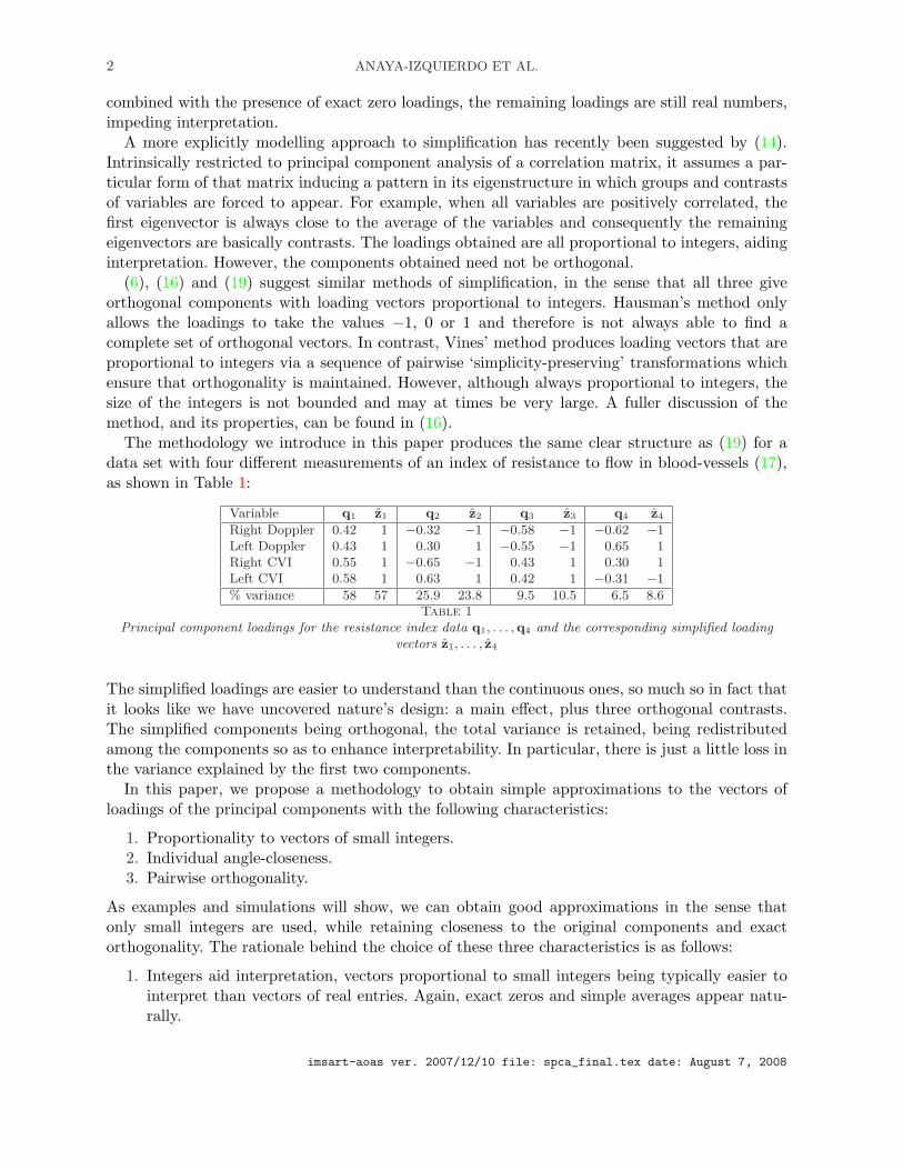
For the exams data, suppose we take α1 = `((1, 1, 1, 1, 1)>). Then the cone C2(π/4, 1) has manyelements, including `((1, 1, 0,−1,−1)>) and `((1, 0, 0, 0,−1)>). Of these, we prefer the first, theiraccuracies being 0.973 and 0.789 respectively. In fact, it can be shown that `((1, 1, 0,−1,−1)>) isthe best simple θ = π/4 approximation to α2 orthogonal to `((1, 1, 1, 1, 1)>).

Note that for the first axis we trivially have q⊥1 = q1, so that ‖q⊥1 ‖ = 1. For the exams datawe have N1(π/4) = 1 and, furthermore, out of all axes of complexity one, `((1, 1, 1, 1, 1)>) is theclosest axis to α1. Therefore, z1 = (1, 1, 1, 1, 1)> is the integer representation of the best simpleθ = π/4 approximation to α1.

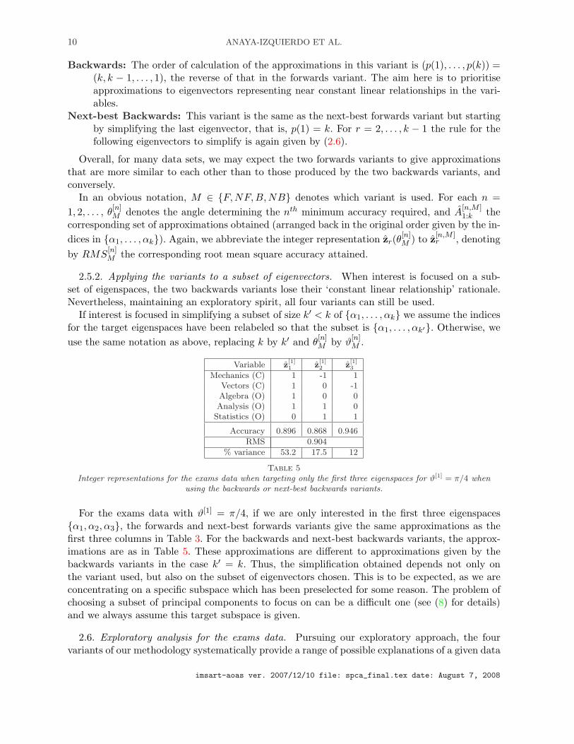
Variable z1(θ) z2(θ) z3(θ) z4(θ) z5(θ)

Mechanics (Closed) 1 -1 1 0 -1Vectors (Closed) 1 -1 -1 0 -1Algebra (Open) 1 0 0 0 4Analysis (Open) 1 1 0 -1 -1

Statistics (Open) 1 1 0 1 -1

Accuracy 0.997 0.973 0.938 0.937 0.974

RMS 0.96

max accuracy ‖q⊥r ‖ 1 0.999 0.99 0.95 0.97

% variance 63.3 14.4 8.9 7.9 5.5

Table 3Integer representations for the examinations data with θ = π/4.

When r = k there is nothing to optimise, because there is a unique simple axis orthogonal toα1, . . . , αk−1 (see Appendix A). We are therefore obliged to take this axis as αk(θ), having nocontrol over its accuracy. However, if αr(θ) is close to to αr for all r < k, then αk(θ) is usuallyclose to αk. We can see an example of this in Table 3, which shows the integer representations ofA1:k(π/4) for the exams data along with the corresponding accuracies attained and their upperbounds.

In general, the complexity of αr(θ) tends to grow as r increases. This happens simply because itbecomes harder for low-complexity axes to satisfy the orthogonality restrictions regardless of theaccuracy required. However, it is always possible to approximate with reasonably high accuracy a



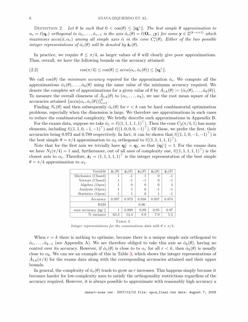
single k-dimensional axis `(q) with a simple axis of low complexity. Figure 1 shows the empiricaldistribution (based on 10000 independent replications) of the minimum complexities N1(θ) fordifferent values of k and cos(θ) when `(q) is sampled from the uniform distribution over the setof all possible axes (see (4).) Clearly, without orthogonality restrictions, accurate approximationsof axes tend not to be very complex.

1 20

0.2

0.4

0.6

0.8

1k=4

cos(

θ)=0

.9

1 20

0.2

0.4

0.6

0.8

1k=8

1 20

0.2

0.4

0.6

0.8

1k=12

1 20

0.2

0.4

0.6

0.8

1k=20

1 2 30

0.2

0.4

0.6

0.8

1

cos(

θ)=0

.95

1 2 30

0.2

0.4

0.6

0.8

1

1 2 30

0.2

0.4

0.6

0.8

1

1 2 30

0.2

0.4

0.6

0.8

1

1 2 3 4 50

0.2

0.4

0.6

cos(

θ)=0

.99

1 2 3 4 5 60

0.2

0.4

0.6

1 2 3 4 5 60

0.2

0.4

0.6

1 2 3 4 5 6 70

0.2

0.4

0.6

Fig 1. Empirical distribution of minimum complexities N1(θ) in simple approximations to k-dimensional axes.

Nevertheless, there is a clear trade-off between accuracy and complexity. Highly accurate ap-proximations usually have high complexity, making the interpretation of the axes more difficult.This is why we choose to control accuracy and then minimise complexity, so our method is biasedtowards simplicity.

2.3. Effect of varying the minimum accuracy required. When θ = π/4 the approximationsA1:k(θ) typically have low complexity overall and so can usually be interpreted. Unless all theeigenspaces are already simple, we might expect the overall complexity of the approximations tosteadily increase with the minimum accuracy required. However, it turns out there is no straight-forward relationship between the complexity of the approximations and cos(θ). Further, althoughless complex axes tend to lead to more interpretable axes, this is not always the case. So, insteadof attempting to find an optimal value of cos(θ) under some criterion, we vary the value of θ toexplore the different approximations obtained. This offers different explanations of the same dataset and so gives more information for interpretation.

The good news is that it is only necessary to explore a discrete set of values of θ. This is becausefor a given θ′, the same approximations will result for any θ such that

cos(θ′) ≤ cos(θ) ≤ minr∈{1,...,k−1}

accu(αr, αr(θ′)).

Thus to fully explore the range of possible approximations it is sufficient to consider the sequenceof angles θ[1], θ[2], . . . where cos(π/4) = cos(θ[1]) < cos(θ[2]) < · · · with

(2.3) cos(θ[n+1]) = minr∈{1,...,k−1}

accu(αr, αr(θ[n])).



For n = 1, 2, . . . , we abbreviate zr(θ[n]) to z[n]r , denoting also by RMS[n] the root mean square

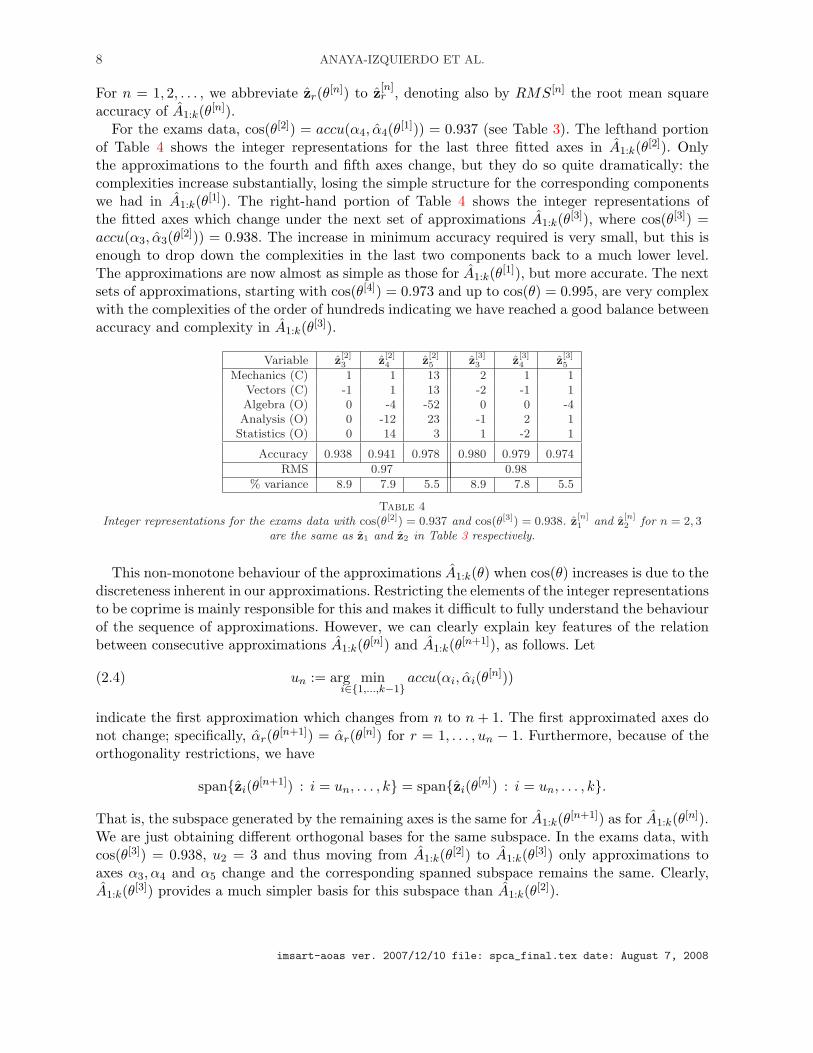
accuracy of A1:k(θ[n]).For the exams data, cos(θ[2]) = accu(α4, α4(θ[1])) = 0.937 (see Table 3). The lefthand portion

of Table 4 shows the integer representations for the last three fitted axes in A1:k(θ[2]). Onlythe approximations to the fourth and fifth axes change, but they do so quite dramatically: thecomplexities increase substantially, losing the simple structure for the corresponding componentswe had in A1:k(θ[1]). The right-hand portion of Table 4 shows the integer representations ofthe fitted axes which change under the next set of approximations A1:k(θ[3]), where cos(θ[3]) =accu(α3, α3(θ[2])) = 0.938. The increase in minimum accuracy required is very small, but this isenough to drop down the complexities in the last two components back to a much lower level.The approximations are now almost as simple as those for A1:k(θ[1]), but more accurate. The nextsets of approximations, starting with cos(θ[4]) = 0.973 and up to cos(θ) = 0.995, are very complexwith the complexities of the order of hundreds indicating we have reached a good balance betweenaccuracy and complexity in A1:k(θ[3]).

Variable z[2]3 z

[2]4 z

[2]5 z

[3]3 z

[3]4 z

[3]5

Mechanics (C) 1 1 13 2 1 1Vectors (C) -1 1 13 -2 -1 1Algebra (O) 0 -4 -52 0 0 -4Analysis (O) 0 -12 23 -1 2 1

Statistics (O) 0 14 3 1 -2 1

Accuracy 0.938 0.941 0.978 0.980 0.979 0.974

RMS 0.97 0.98

% variance 8.9 7.9 5.5 8.9 7.8 5.5

Table 4Integer representations for the exams data with cos(θ[2]) = 0.937 and cos(θ[3]) = 0.938. z

[n]1 and z

[n]2 for n = 2, 3

are the same as z1 and z2 in Table 3 respectively.

This non-monotone behaviour of the approximations A1:k(θ) when cos(θ) increases is due to thediscreteness inherent in our approximations. Restricting the elements of the integer representationsto be coprime is mainly responsible for this and makes it difficult to fully understand the behaviourof the sequence of approximations. However, we can clearly explain key features of the relationbetween consecutive approximations A1:k(θ[n]) and A1:k(θ[n+1]), as follows. Let

(2.4) un := arg mini∈{1,...,k−1}

accu(αi, αi(θ[n]))

indicate the first approximation which changes from n to n + 1. The first approximated axes donot change; specifically, αr(θ[n+1]) = αr(θ[n]) for r = 1, . . . , un − 1. Furthermore, because of theorthogonality restrictions, we have

span{zi(θ[n+1]) : i = un, . . . , k} = span{zi(θ[n]) : i = un, . . . , k}.

That is, the subspace generated by the remaining axes is the same for A1:k(θ[n+1]) as for A1:k(θ[n]).We are just obtaining different orthogonal bases for the same subspace. In the exams data, withcos(θ[3]) = 0.938, u2 = 3 and thus moving from A1:k(θ[2]) to A1:k(θ[3]) only approximations toaxes α3, α4 and α5 change and the corresponding spanned subspace remains the same. Clearly,A1:k(θ[3]) provides a much simpler basis for this subspace than A1:k(θ[2]).



2.4. Targeting a subset of eigenvectors. Often, interest is focused on just a subset of theeigenvectors, typically the first few dominant ones. Again, subsuming a permutation, there is noloss of generality in considering this case.

If we want to simplify the first k′ < k eigenspaces {α1, . . . , αk′}, we proceed as above bysimplifying this subset only and varying the minimum accuracy required for this case, whichwe denote now by cos(ϑ). The range of possible approximations, denoted by A1:k′(ϑ), will bedetermined by the sequence of angles ϑ[1], ϑ[2], ... defined by

(2.5) ϑ[1] = π/4, cos(ϑ[n+1]) = minr∈{1,...,k′}

accu(αr, αr(ϑ[n])) (n ≥ 1).

This is a subsequence of the full sequence (2.3) where we skip the approximations A1:k(θ[n])for which the target eigenvectors do not change. Note that the last approximation computed inA1:k′(ϑ) is not determined by those already fitted, as it was in the complete case k′ = k.

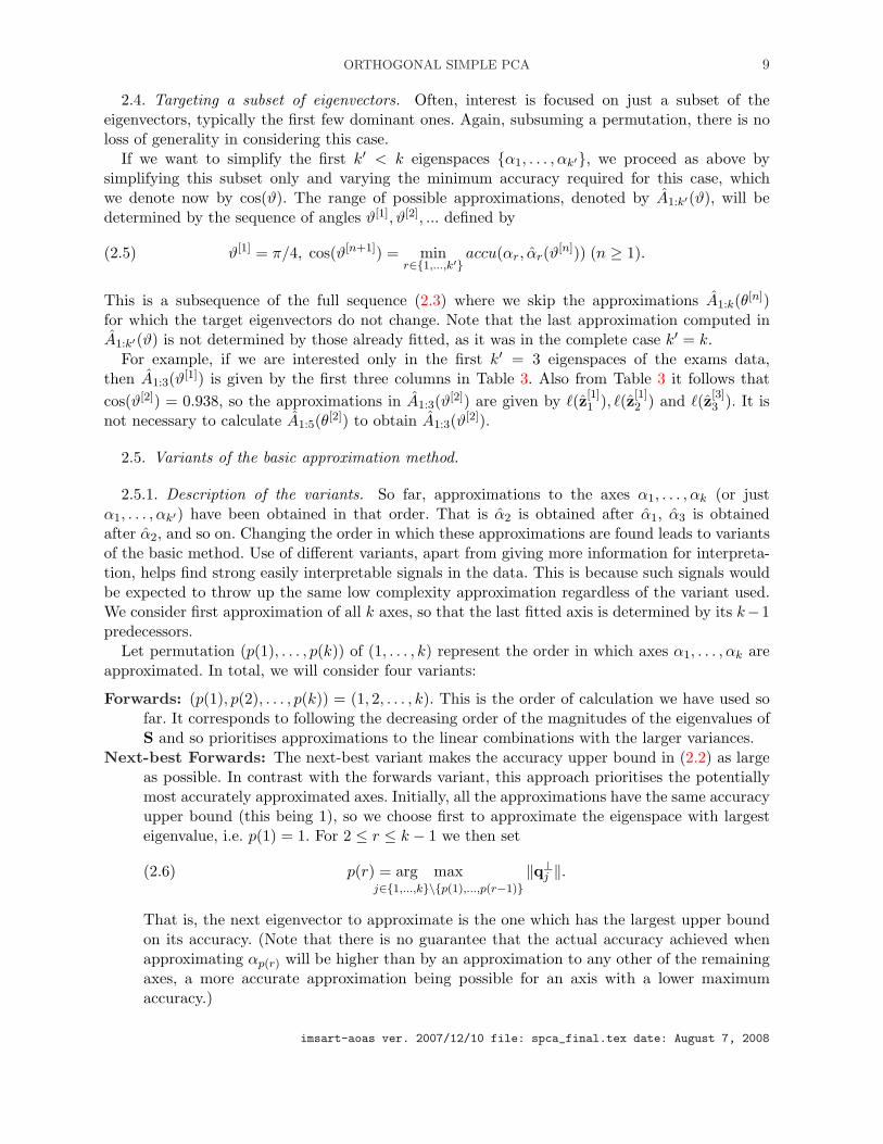
For example, if we are interested only in the first k′ = 3 eigenspaces of the exams data,then A1:3(ϑ[1]) is given by the first three columns in Table 3. Also from Table 3 it follows thatcos(ϑ[2]) = 0.938, so the approximations in A1:3(ϑ[2]) are given by `(z[1]

1 ), `(z[1]2 ) and `(z[3]

3 ). It isnot necessary to calculate A1:5(θ[2]) to obtain A1:3(ϑ[2]).

2.5. Variants of the basic approximation method.

2.5.1. Description of the variants. So far, approximations to the axes α1, . . . , αk (or justα1, . . . , αk′) have been obtained in that order. That is α2 is obtained after α1, α3 is obtainedafter α2, and so on. Changing the order in which these approximations are found leads to variantsof the basic method. Use of different variants, apart from giving more information for interpreta-tion, helps find strong easily interpretable signals in the data. This is because such signals wouldbe expected to throw up the same low complexity approximation regardless of the variant used.We consider first approximation of all k axes, so that the last fitted axis is determined by its k−1predecessors.

Let permutation (p(1), . . . , p(k)) of (1, . . . , k) represent the order in which axes α1, . . . , αk areapproximated. In total, we will consider four variants:

Forwards: (p(1), p(2), . . . , p(k)) = (1, 2, . . . , k). This is the order of calculation we have used sofar. It corresponds to following the decreasing order of the magnitudes of the eigenvalues ofS and so prioritises approximations to the linear combinations with the larger variances.

Next-best Forwards: The next-best variant makes the accuracy upper bound in (2.2) as largeas possible. In contrast with the forwards variant, this approach prioritises the potentiallymost accurately approximated axes. Initially, all the approximations have the same accuracyupper bound (this being 1), so we choose first to approximate the eigenspace with largesteigenvalue, i.e. p(1) = 1. For 2 ≤ r ≤ k − 1 we then set

(2.6) p(r) = arg maxj∈{1,...,k}\{p(1),...,p(r−1)}

‖q⊥j ‖.

That is, the next eigenvector to approximate is the one which has the largest upper boundon its accuracy. (Note that there is no guarantee that the actual accuracy achieved whenapproximating αp(r) will be higher than by an approximation to any other of the remainingaxes, a more accurate approximation being possible for an axis with a lower maximumaccuracy.)



Backwards: The order of calculation of the approximations in this variant is (p(1), . . . , p(k)) =(k, k − 1, . . . , 1), the reverse of that in the forwards variant. The aim here is to prioritiseapproximations to eigenvectors representing near constant linear relationships in the vari-ables.

Next-best Backwards: This variant is the same as the next-best forwards variant but startingby simplifying the last eigenvector, that is, p(1) = k. For r = 2, . . . , k − 1 the rule for thefollowing eigenvectors to simplify is again given by (2.6).

Overall, for many data sets, we may expect the two forwards variants to give approximationsthat are more similar to each other than to those produced by the two backwards variants, andconversely.

In an obvious notation, M ∈ {F,NF, B, NB} denotes which variant is used. For each n =1, 2, . . . , θ

[n]M denotes the angle determining the nth minimum accuracy required, and A

[n,M ]1:k the

corresponding set of approximations obtained (arranged back in the original order given by the in-dices in {α1, . . . , αk}). Again, we abbreviate the integer representation zr(θ

[n]M ) to z[n,M ]

r , denotingby RMS

[n]M the corresponding root mean square accuracy attained.

2.5.2. Applying the variants to a subset of eigenvectors. When interest is focused on a sub-set of eigenspaces, the two backwards variants lose their ‘constant linear relationship’ rationale.Nevertheless, maintaining an exploratory spirit, all four variants can still be used.

If interest is focused in simplifying a subset of size k′ < k of {α1, . . . , αk} we assume the indicesfor the target eigenspaces have been relabeled so that the subset is {α1, . . . , αk′}. Otherwise, weuse the same notation as above, replacing k by k′ and θ

[n]M by ϑ

[n]M .

Variable z[1]1 z

[1]2 z

[1]3

Mechanics (C) 1 -1 1Vectors (C) 1 0 -1Algebra (O) 1 0 0Analysis (O) 1 1 0

Statistics (O) 0 1 1

Accuracy 0.896 0.868 0.946

RMS 0.904

% variance 53.2 17.5 12

Table 5Integer representations for the exams data when targeting only the first three eigenspaces for ϑ[1] = π/4 when

using the backwards or next-best backwards variants.

For the exams data with ϑ[1] = π/4, if we are only interested in the first three eigenspaces{α1, α2, α3}, the forwards and next-best forwards variants give the same approximations as thefirst three columns in Table 3. For the backwards and next-best backwards variants, the approx-imations are as in Table 5. These approximations are different to approximations given by thebackwards variants in the case k′ = k. Thus, the simplification obtained depends not only onthe variant used, but also on the subset of eigenvectors chosen. This is to be expected, as we areconcentrating on a specific subspace which has been preselected for some reason. The problem ofchoosing a subset of principal components to focus on can be a difficult one (see (8) for details)and we always assume this target subspace is given.

2.6. Exploratory analysis for the exams data. Pursuing our exploratory approach, the fourvariants of our methodology systematically provide a range of possible explanations of a given data



set, corresponding to its projections onto different sets of orthogonal simple axes. As noted in theintroduction, these explanations can vary on many factors, including interpretability, simplicity,accuracy, subject matter considerations and suboptimality criteria. Accordingly, different userscan be lead to make different choices.

In this case, for the complete set of eigenvectors derived from the exams data, we suggest thefollowing shortlist:

Forwards: We feel that approximation A[1,F ]1:5 (Table 3) is the simplest and most interpretable

obtained using this variant. The overall accuracy attained is quite high, RMS[1]F being 0.96.

In particular, the percentage of variance explained by the first three components (86.6%)is close to the corresponding optimal percentage of variance explained (87.3%). An almostequally good approximation is A

[3,F ]1:5 (Table 4), with RMS

[3]F = 0.98, while the variance

explained by the first three components is virtually identical under both approximations.The difference between both approximations is just the basis for the space spanned by thelast 3 components.Overall, it seems that A

[1,F ]1:5 has the edge, its interpretation being particularly straight-

forward. Algebra turning out to behave differently from the other two open-book exams,Analysis and Statistics, it is helpful here to use ‘open’ to refer to this latter pair alone. Thesimple components explain the total variability in the data – in other words, they answerthe question: ‘why do students perform differently in the 5 exams?’ – as follows:

α1: Differences in overall mathematical ability.

α2: Differences between open- and closed-book exam performances.

α3: Differences between closed-book exam performances.

α4: Differences between open-book exam performances.

α5: Differences between performance in Algebra and all other subjects.

Next-best Forwards: It appears the best approximation for this variant is A[1,NF ]1:5 , for which

the order in which the approximations were obtained is (p(1), . . . , p(5)) = (1, 4, 2, 5, 3). Now,A

[1,NF ]1:5 happens to coincide with A

[1,F ]1:5 (Table 3). This is evidence of a strong signal in the

data. For example, the approximations to α4 and α5 obtained by A[1,NF ]1:5 are the same

as those obtained by A[1,F ]1:5 despite some orthogonality restrictions being dropped, similar

remarks applying to α2 and α3 on reversing the roles of the variants.A close contender is A

[3,NF ]1:5 , where cos(θ[3]

NF ) = 0.959. In fact, A[3,NF ]1:5 coincides with A

[3,F ]1:5 ,

discussed above, again signalling structure in the data. Using a minimum accuracy ofcos(θ[2]

NF ) = 0.937 we obtain approximations (not shown) for which the interpretation inthe approximated component 5 is quite different, and in our opinion worse, compared toA

[1,NF ]1:5 and A

[3,NF ]1:5 . The remaining approximations under this method are rather complex

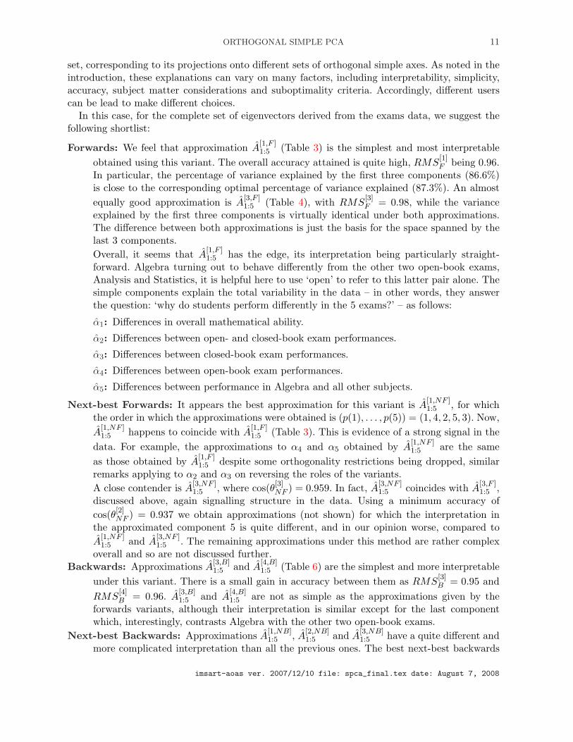
overall and so are not discussed further.Backwards: Approximations A

[3,B]1:5 and A

[4,B]1:5 (Table 6) are the simplest and more interpretable

under this variant. There is a small gain in accuracy between them as RMS[3]B = 0.95 and

RMS[4]B = 0.96. A

[3,B]1:5 and A

[4,B]1:5 are not as simple as the approximations given by the

forwards variants, although their interpretation is similar except for the last componentwhich, interestingly, contrasts Algebra with the other two open-book exams.

Next-best Backwards: Approximations A[1,NB]1:5 , A

[2,NB]1:5 and A

[3,NB]1:5 have a quite different and

more complicated interpretation than all the previous ones. The best next-best backwards



Var z[3,B]1 z

[3,B]2 z

[4,B]1 z

[4,B]2 z

[4,B]3 z

[4,B]4 z

[4,B]5

Mechanics 3 -1 3 -2 1 0 0Vectors 3 -1 3 -2 -1 0 0Algebra 2 1 4 1 0 0 2Analysis 2 1 4 1 0 1 -1

Statistics 2 1 4 1 0 -1 -1

Accuracy 0.966 0.928 0.996 0.953 0.938 0.937 0.959

RMS 0.95 0.96

% variance 60.2 17.3 63.2 14.3 8.9 7.9 5.7

Table 6Integer representations for the examinations data with cos(θ[3]) = 0.898 and cos(θ[4]) = 0.928. z

[3,B]r = z

[4,B]r for

r = 3, 4, 5.

solution we obtained was A[4,NB]1:5 . This turned out to coincide with A

[2,NF ]1:5 , despite the

order of calculation in those approximations being different, ((5, 1, 4, 3, 2) and (1, 4, 5, 3, 2)respectively), again indicating clear structure in the data.

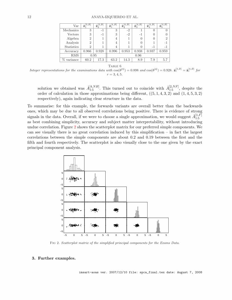
To summarise: for this example, the forwards variants are overall better than the backwardsones, which may be due to all observed correlations being positive. There is evidence of strongsignals in the data. Overall, if we were to choose a single approximation, we would suggest A

[1,F ]1:5

as best combining simplicity, accuracy and subject matter interpretability, without introducingundue correlation. Figure 2 shows the scatterplot matrix for our preferred simple components. Wecan see visually there is no great correlation induced by this simplification – in fact the largestcorrelations between the simple components are about 0.2 and 0.19 between the first and thefifth and fourth respectively. The scatterplot is also visually close to the one given by the exactprincipal component analysis.

−5 0 5−5 0 5−5 0 5−5 0 5−5 0 5

−5

0

5

−5

0

5

−5

0

5

−5

0

5

Fig 2. Scatterplot matrix of the simplified principal components for the Exams Data.

3. Further examples.



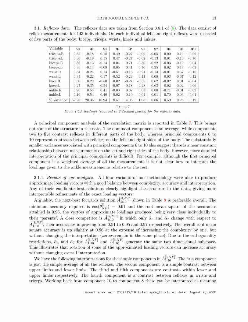
3.1. Reflexes data. The reflexes data are taken from Section 3.8.1 of (8). The data consist ofreflex measurements for 143 individuals. On each individual left and right reflexes were recordedof five parts of the body: biceps, triceps, wrists, knees and ankles.

Variable q1 q2 q3 q4 q5 q6 q7 q8 q9 q10

triceps.R 0.35 -0.18 0.18 0.49 -0.27 -0.06 -0.05 0.00 0.10 0.69triceps.L 0.36 -0.19 0.15 0.47 -0.27 -0.02 -0.13 0.01 -0.13 -0.70

biceps.R 0.36 -0.13 -0.14 0.04 0.71 -0.50 -0.22 -0.03 -0.19 0.04biceps.L 0.39 -0.14 -0.09 0.05 0.41 0.70 0.35 0.02 0.19 -0.03

wrist.R 0.34 -0.24 0.14 -0.51 -0.16 -0.21 -0.13 -0.01 0.67 -0.10wrist.L 0.34 -0.22 0.17 -0.52 -0.23 0.11 0.08 0.03 -0.67 0.12

knee.R 0.30 0.29 -0.50 0.02 -0.24 -0.35 0.62 -0.02 0.01 -0.04knee.L 0.27 0.35 -0.54 -0.07 -0.18 0.28 -0.63 0.02 -0.02 0.06

ankle.R 0.20 0.53 0.41 -0.03 0.07 0.03 0.00 -0.71 -0.01 -0.02ankle.L 0.19 0.54 0.40 -0.02 0.10 -0.04 0.01 0.70 0.03 -0.01

% variance 52.23 20.36 10.94 8.57 4.96 1.08 0.86 0.59 0.23 0.19

Table 7Exact PCA loadings (rounded to 2 decimal places) for the reflexes data.

A principal component analysis of the correlation matrix is reported in Table 7. This bringsout some of the structure in the data. The dominant component is an average, while componentstwo to five contrast reflexes in different parts of the body, whereas principal components 6 to10 represent contrasts between reflexes on the left and right sides of the body. The substantiallysmaller variances associated with principal components 6 to 10 also suggest there is a near constantrelationship between measurements on the left and right sides of the body. However, more detailedinterpretation of the principal components is difficult. For example, although the first principalcomponent is a weighted average of all the measurements it is not clear how to interpret theloadings given to the ankle measurements relative to the rest.

3.1.1. Results of our analyses. All four variants of our methodology were able to produceapproximate loading vectors with a good balance between complexity, accuracy and interpretation.Any of their candidate best solutions clearly highlight the structure in the data, giving moreinterpretable refinements of the exact loading vectors.

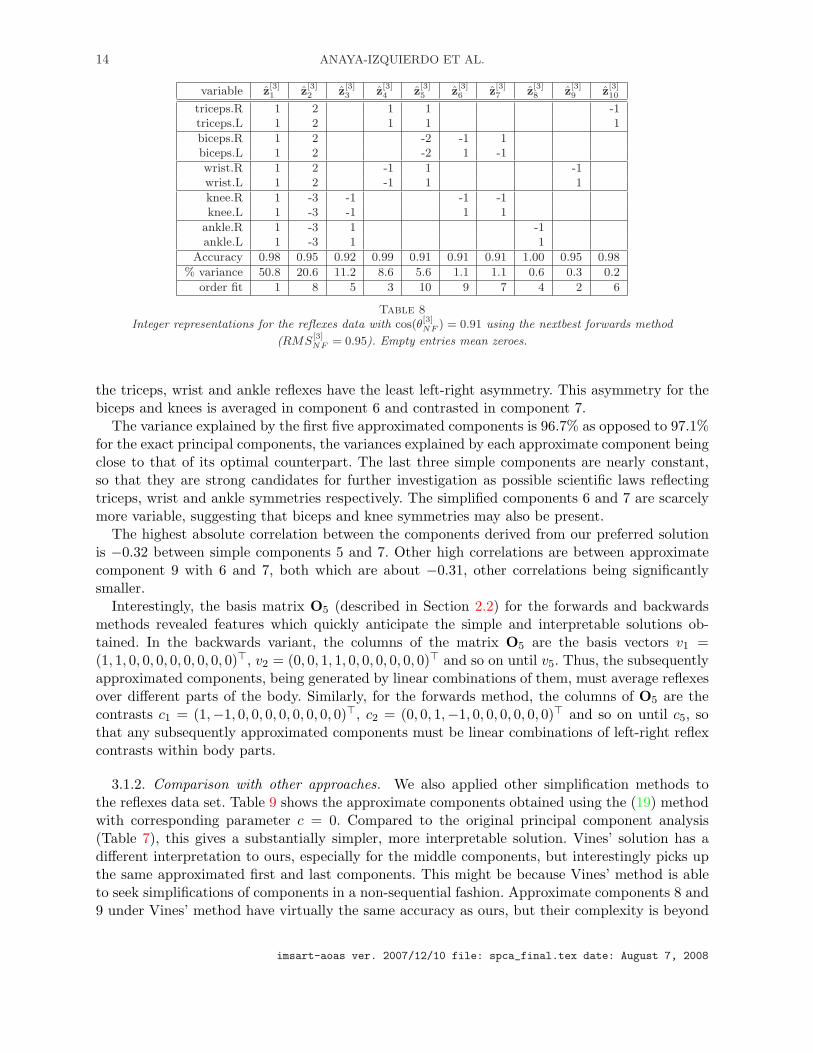
Arguably, the next-best forwards solution A[3,NF ]1:10 shown in Table 8 is preferable overall. The

minimum accuracy required is cos(θ[3]NF ) = 0.91 and the root mean square of the accuracies

attained is 0.95, the vectors of approximate loadings produced being very close individually totheir ‘parents’. A close competitor is A

[5,NF ]1:10 in which only α6 and α7 change with respect to

A[3,NF ]1:10 , their accuracies improving from 0.91 to 0.95 and 0.97 respectively. The overall root mean

square accuracy is up slightly at 0.96 at the expense of increasing the complexity by one, butwithout changing the interpretation (zeroes remain in the same place). Due to the orthogonalityrestrictions, α6 and α7 for A

[3,NF ]1:10 and A

[5,NF ]1:10 generate the same two dimensional subspace.

This illustrates that rotation of some of the approximated loading vectors can increase accuracywithout changing overall interpretation.

We have the following interpretations for the simple components in A[3,NF ]1:10 . The first component

is just the simple average of all the reflexes. The second component is a simple contrast betweenupper limbs and lower limbs. The third and fifth components are contrasts within lower andupper limbs respectively. The fourth component is a contrast between reflexes in wrists andtriceps. Working back from component 10 to component 8 these can be interpreted as meaning



variable z[3]1 z

[3]2 z

[3]3 z

[3]4 z

[3]5 z

[3]6 z

[3]7 z

[3]8 z

[3]9 z

[3]10

triceps.R 1 2 1 1 -1triceps.L 1 2 1 1 1

biceps.R 1 2 -2 -1 1biceps.L 1 2 -2 1 -1

wrist.R 1 2 -1 1 -1wrist.L 1 2 -1 1 1

knee.R 1 -3 -1 -1 -1knee.L 1 -3 -1 1 1

ankle.R 1 -3 1 -1ankle.L 1 -3 1 1

Accuracy 0.98 0.95 0.92 0.99 0.91 0.91 0.91 1.00 0.95 0.98

% variance 50.8 20.6 11.2 8.6 5.6 1.1 1.1 0.6 0.3 0.2

order fit 1 8 5 3 10 9 7 4 2 6

Table 8Integer representations for the reflexes data with cos(θ

[3]NF ) = 0.91 using the nextbest forwards method

(RMS[3]NF = 0.95). Empty entries mean zeroes.

the triceps, wrist and ankle reflexes have the least left-right asymmetry. This asymmetry for thebiceps and knees is averaged in component 6 and contrasted in component 7.

The variance explained by the first five approximated components is 96.7% as opposed to 97.1%for the exact principal components, the variances explained by each approximate component beingclose to that of its optimal counterpart. The last three simple components are nearly constant,so that they are strong candidates for further investigation as possible scientific laws reflectingtriceps, wrist and ankle symmetries respectively. The simplified components 6 and 7 are scarcelymore variable, suggesting that biceps and knee symmetries may also be present.

The highest absolute correlation between the components derived from our preferred solutionis −0.32 between simple components 5 and 7. Other high correlations are between approximatecomponent 9 with 6 and 7, both which are about −0.31, other correlations being significantlysmaller.

Interestingly, the basis matrix O5 (described in Section 2.2) for the forwards and backwardsmethods revealed features which quickly anticipate the simple and interpretable solutions ob-tained. In the backwards variant, the columns of the matrix O5 are the basis vectors v1 =(1, 1, 0, 0, 0, 0, 0, 0, 0, 0)>, v2 = (0, 0, 1, 1, 0, 0, 0, 0, 0, 0)> and so on until v5. Thus, the subsequentlyapproximated components, being generated by linear combinations of them, must average reflexesover different parts of the body. Similarly, for the forwards method, the columns of O5 are thecontrasts c1 = (1,−1, 0, 0, 0, 0, 0, 0, 0, 0)>, c2 = (0, 0, 1,−1, 0, 0, 0, 0, 0, 0)> and so on until c5, sothat any subsequently approximated components must be linear combinations of left-right reflexcontrasts within body parts.

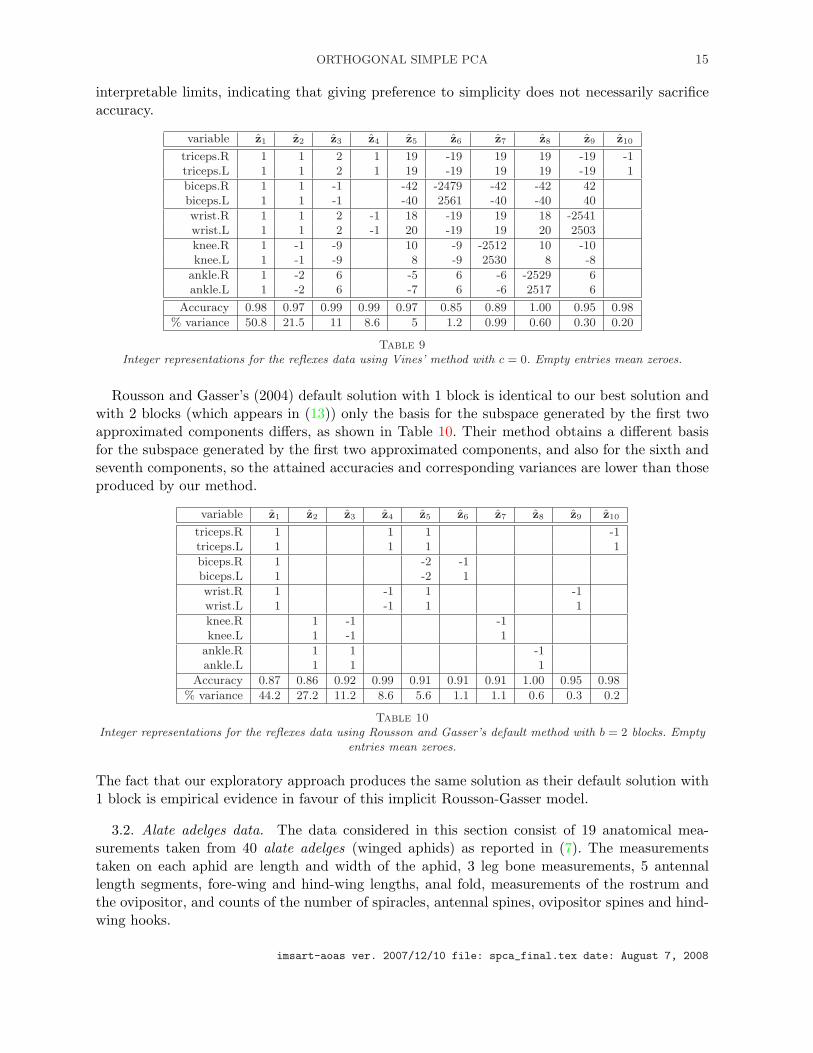
3.1.2. Comparison with other approaches. We also applied other simplification methods tothe reflexes data set. Table 9 shows the approximate components obtained using the (19) methodwith corresponding parameter c = 0. Compared to the original principal component analysis(Table 7), this gives a substantially simpler, more interpretable solution. Vines’ solution has adifferent interpretation to ours, especially for the middle components, but interestingly picks upthe same approximated first and last components. This might be because Vines’ method is ableto seek simplifications of components in a non-sequential fashion. Approximate components 8 and9 under Vines’ method have virtually the same accuracy as ours, but their complexity is beyond



interpretable limits, indicating that giving preference to simplicity does not necessarily sacrificeaccuracy.

variable z1 z2 z3 z4 z5 z6 z7 z8 z9 z10

triceps.R 1 1 2 1 19 -19 19 19 -19 -1triceps.L 1 1 2 1 19 -19 19 19 -19 1

biceps.R 1 1 -1 -42 -2479 -42 -42 42biceps.L 1 1 -1 -40 2561 -40 -40 40

wrist.R 1 1 2 -1 18 -19 19 18 -2541wrist.L 1 1 2 -1 20 -19 19 20 2503

knee.R 1 -1 -9 10 -9 -2512 10 -10knee.L 1 -1 -9 8 -9 2530 8 -8

ankle.R 1 -2 6 -5 6 -6 -2529 6ankle.L 1 -2 6 -7 6 -6 2517 6

Accuracy 0.98 0.97 0.99 0.99 0.97 0.85 0.89 1.00 0.95 0.98

% variance 50.8 21.5 11 8.6 5 1.2 0.99 0.60 0.30 0.20

Table 9Integer representations for the reflexes data using Vines’ method with c = 0. Empty entries mean zeroes.

Rousson and Gasser’s (2004) default solution with 1 block is identical to our best solution andwith 2 blocks (which appears in (13)) only the basis for the subspace generated by the first twoapproximated components differs, as shown in Table 10. Their method obtains a different basisfor the subspace generated by the first two approximated components, and also for the sixth andseventh components, so the attained accuracies and corresponding variances are lower than thoseproduced by our method.

variable z1 z2 z3 z4 z5 z6 z7 z8 z9 z10

triceps.R 1 1 1 -1triceps.L 1 1 1 1

biceps.R 1 -2 -1biceps.L 1 -2 1

wrist.R 1 -1 1 -1wrist.L 1 -1 1 1

knee.R 1 -1 -1knee.L 1 -1 1

ankle.R 1 1 -1ankle.L 1 1 1

Accuracy 0.87 0.86 0.92 0.99 0.91 0.91 0.91 1.00 0.95 0.98

% variance 44.2 27.2 11.2 8.6 5.6 1.1 1.1 0.6 0.3 0.2

Table 10Integer representations for the reflexes data using Rousson and Gasser’s default method with b = 2 blocks. Empty

entries mean zeroes.

The fact that our exploratory approach produces the same solution as their default solution with1 block is empirical evidence in favour of this implicit Rousson-Gasser model.

3.2. Alate adelges data. The data considered in this section consist of 19 anatomical mea-surements taken from 40 alate adelges (winged aphids) as reported in (7). The measurementstaken on each aphid are length and width of the aphid, 3 leg bone measurements, 5 antennallength segments, fore-wing and hind-wing lengths, anal fold, measurements of the rostrum andthe ovipositor, and counts of the number of spiracles, antennal spines, ovipositor spines and hind-wing hooks.



Variable q1 q2 q3 q4

Length 0.25 -0.03 -0.02 0.07Width 0.26 -0.07 -0.01 0.10

Fore-wing 0.26 -0.03 0.05 0.07Hind-wing 0.26 -0.09 -0.03 0.00

Spiracles 0.16 0.41 0.19 -0.62Antseg 1 0.24 0.18 -0.04 -0.01Antseg 2 0.25 0.16 0.00 0.02Antseg 3 0.23 -0.24 -0.05 0.11Antseg 4 0.24 -0.04 -0.16 0.01Antseg 5 0.25 0.03 -0.10 -0.02

Ant-spines -0.13 0.20 -0.93 -0.17Tarsus 3 0.26 -0.01 -0.03 0.18Tibia 3 0.26 -0.03 -0.08 0.20

Femur 3 0.26 -0.07 -0.12 0.19Rostrum 0.25 0.01 -0.07 0.04

Ovipositor 0.20 0.40 0.02 0.06Ov-spines 0.11 0.55 0.15 0.04

Fold -0.19 0.35 -0.04 0.49Hooks 0.20 -0.28 -0.05 -0.45

% variance 73 12.5 3.9 2.6

Table 11Exact principal component analysis loadings (rounded to 2 decimal places) for the alate adelges data.

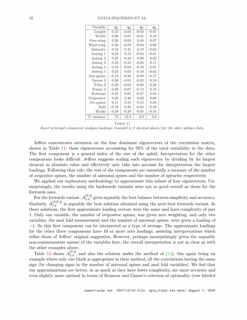
Jeffers concentrates attention on the four dominant eigenvectors of the correlation matrix,shown in Table 11, these eigenvectors accounting for 92% of the total variability in the data.The first component is a general index of the size of the aphid. Interpretation for the othercomponents looks difficult. Jeffers suggests scaling each eigenvector by dividing by its largestelement in absolute value and effectively only take into account for interpretation the largestloadings. Following that rule, the rest of the components are essentially a measure of the numberof ovipositor spines, the number of antennal spines and the number of spiracles respectively.

We applied our exploratory methodology to approximate this subset of four eigenvectors. Un-surprisingly, the results using the backwards variants were not so good overall as those for theforwards ones.

For the forwards variant, A[F,4]1:4 gives arguably the best balance between simplicity and accuracy.

Similarly, A[NF,4]1:4 is arguably the best solution obtained using the next-best forwards variant. In

these solutions, the first approximate loading vectors were the same and have complexity of just1. Only one variable, the number of ovipositor spines, was given zero weighting, and only twovariables, the anal fold measurement and the number of antennal spines, were given a loading of−1. So this first component can be interpreted as a type of average. The approximate loadingsfor the other three components have 10 or more zero loadings, assisting interpretations whichrefine those of Jeffers’ original suggestion. However, perhaps unsurprisingly given the arguablynon-commensurate nature of the variables here, the overall interpretation is not as clear as withthe other examples above.

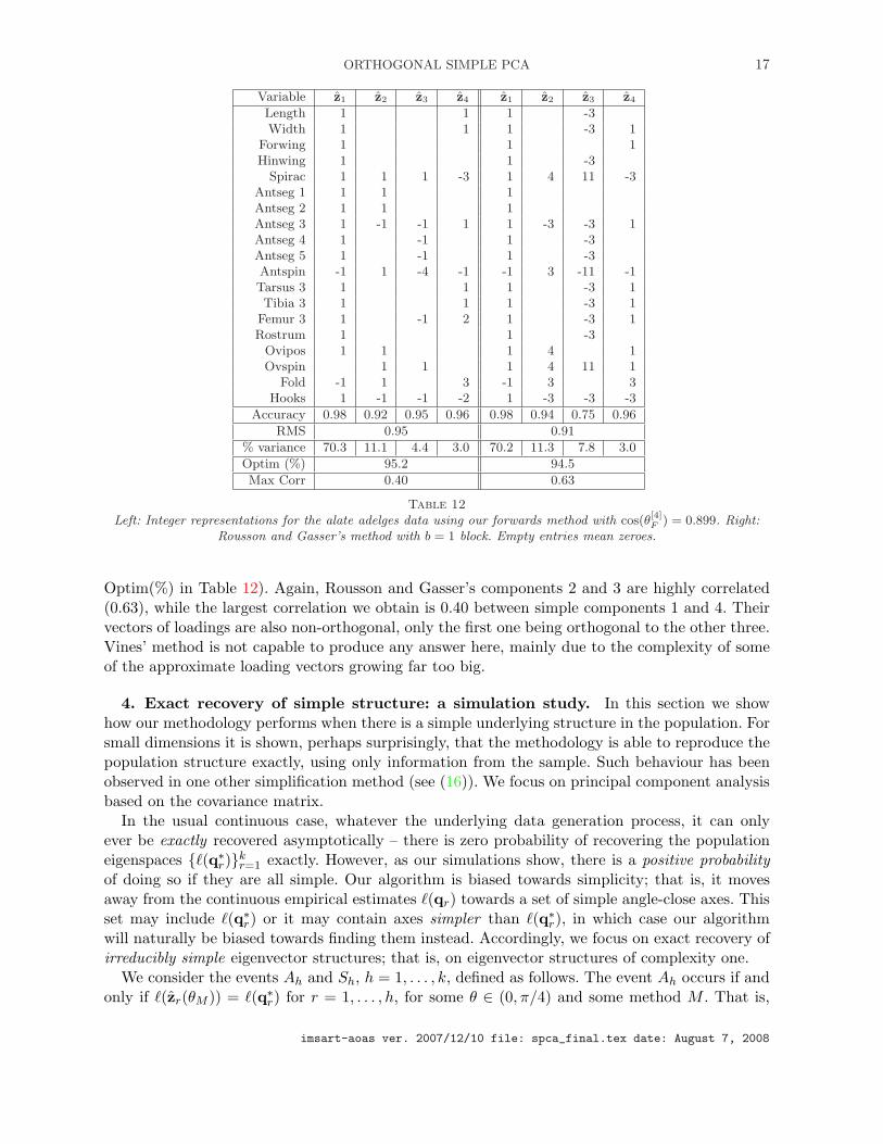
Table 12 shows A[F,4]1:4 and also the solution under the method of (14), this again being an

example where only one block is appropriate in their method, all the correlations having the samesign (by changing signs in the number of antennal spines and anal fold variables). We feel thatour approximations are better, in as much as they have lower complexity, are more accurate andeven slightly more optimal in terms of Rousson and Gasser’s criterion of optimality (row labeled



Variable z1 z2 z3 z4 z1 z2 z3 z4

Length 1 1 1 -3Width 1 1 1 -3 1

Forwing 1 1 1Hinwing 1 1 -3

Spirac 1 1 1 -3 1 4 11 -3Antseg 1 1 1 1Antseg 2 1 1 1Antseg 3 1 -1 -1 1 1 -3 -3 1Antseg 4 1 -1 1 -3Antseg 5 1 -1 1 -3Antspin -1 1 -4 -1 -1 3 -11 -1Tarsus 3 1 1 1 -3 1Tibia 3 1 1 1 -3 1

Femur 3 1 -1 2 1 -3 1Rostrum 1 1 -3

Ovipos 1 1 1 4 1Ovspin 1 1 1 4 11 1

Fold -1 1 3 -1 3 3Hooks 1 -1 -1 -2 1 -3 -3 -3

Accuracy 0.98 0.92 0.95 0.96 0.98 0.94 0.75 0.96

RMS 0.95 0.91

% variance 70.3 11.1 4.4 3.0 70.2 11.3 7.8 3.0

Optim (%) 95.2 94.5

Max Corr 0.40 0.63

Table 12Left: Integer representations for the alate adelges data using our forwards method with cos(θ

[4]F ) = 0.899. Right:

Rousson and Gasser’s method with b = 1 block. Empty entries mean zeroes.

Optim(%) in Table 12). Again, Rousson and Gasser’s components 2 and 3 are highly correlated(0.63), while the largest correlation we obtain is 0.40 between simple components 1 and 4. Theirvectors of loadings are also non-orthogonal, only the first one being orthogonal to the other three.Vines’ method is not capable to produce any answer here, mainly due to the complexity of someof the approximate loading vectors growing far too big.

4. Exact recovery of simple structure: a simulation study. In this section we showhow our methodology performs when there is a simple underlying structure in the population. Forsmall dimensions it is shown, perhaps surprisingly, that the methodology is able to reproduce thepopulation structure exactly, using only information from the sample. Such behaviour has beenobserved in one other simplification method (see (16)). We focus on principal component analysisbased on the covariance matrix.

In the usual continuous case, whatever the underlying data generation process, it can onlyever be exactly recovered asymptotically – there is zero probability of recovering the populationeigenspaces {`(q∗r)}k

r=1 exactly. However, as our simulations show, there is a positive probabilityof doing so if they are all simple. Our algorithm is biased towards simplicity; that is, it movesaway from the continuous empirical estimates `(qr) towards a set of simple angle-close axes. Thisset may include `(q∗r) or it may contain axes simpler than `(q∗r), in which case our algorithmwill naturally be biased towards finding them instead. Accordingly, we focus on exact recovery ofirreducibly simple eigenvector structures; that is, on eigenvector structures of complexity one.

We consider the events Ah and Sh, h = 1, . . . , k, defined as follows. The event Ah occurs if andonly if `(zr(θM )) = `(q∗r) for r = 1, . . . , h, for some θ ∈ (0, π/4) and some method M . That is,



the first h population eigenspaces are recovered exactly by any of the four variants for any of itsminimum accuracies. This is consistent with the analysis of the examples where all the variantswere applied to the data and the best looking results selected. The event Sh occurs if and onlyif `(qr) is closer to `(q∗r) than any other eigenspace `(q∗s) s = 1, . . . , k, s 6= r, this holding forr = 1, . . . , h. That is, if the first h sample eigenspaces appear in the same order as their populationcounterparts.

For exact recovery, we focus on the conditional probabilities P (Ah | Sh) for h = 1, . . . , k.We condition on Sh as it would be inappropriate to check if Ah has occurred when Sh has not.As h increases, these probabilities evaluate the progressive effectiveness of our methodology inrecovering the population eigenvectors.

We performed the following simulation study. For a range of matrices Z∗ = [z∗1, . . . , z∗k], wherez∗1, . . . , z∗k are integer orthogonal vectors of dimension k, and of spectra Λ∗ := diag(λ∗1, . . . , λ∗k),where λ∗1 > λ∗2 > . . . > λ∗k > 0, we constructed the corresponding population covariance matrixΣ∗ = Q∗Λ∗(Q∗)T where Q∗ is just Z∗ with its columns normalised to have unit length. Wesimulated n observations from a k-variate normal distribution with mean zero and covarianceΣ∗. We computed the eigenvalues Λ := diag(λ1, . . . , λk) where λ1 > λ2 > . . . > λk > 0 andeigenvectors Q = [q1, . . . ,qk] of the usual empirical covariance matrix S. We calculated Z(θM ) =[z1, . . . , zk] for all four variants and for θ in the accuracy range of [cos(π/4), cos(π/10)]. Experienceshowed this is a good enough range to explore. We replicated independently 1000 times.

For illustration purposes, we focus only on the case k = 8. Three representative structures ofirreducibly simple eigenvectors were studied: the identity Z∗id structure, the Hadamard structuredefined by

Z∗h,8 =

(Z∗h,4 Z∗h,4

Z∗h,4 −Z∗h,4

),

where

Z∗h,4 =

(Z∗h,2 Z∗h,2

Z∗h,2 −Z∗h,2

)and Z∗h,2 =

(1 11 −1

),

and a mixed structure defined by

Z∗mix,8 =

(Z∗h,4 00 Z∗h,4

).

The aim is to see how our methodology performs when, with high probability, sample eigenspacesappear in the same order as their population counterparts. To this end, we use well-separatedeigenvalues – specifically, those occurring in geometrically increasing spectra, that is (λ∗1, . . . , λ∗k) =(rk−1, . . . , r, 1) for r = 1.5 or 2 – and n = 100, for which the estimated value of any P (Sh) wasnever below 0.9.

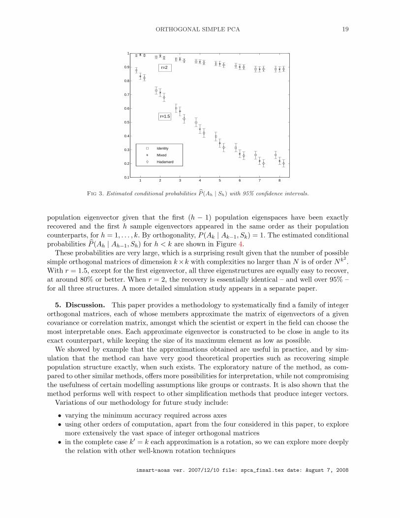
The estimated conditional probabilities P (Ah | Sh) are shown in Figure 3 together with cor-responding pointwise asymptotic 95% confidence intervals. First, we note these probabilities aresurprisingly large, at least for the first few components. As expected, there is a better recoverywhen the ratio between consecutive eigenvalues increases. When r = 1.5, there is better overallrecovery of the identity structure, the mixed and Hadamard structures being progressively a littlemore difficult to recover. This maybe because a sparse structure is a bit easier to recover exactlywhen the eigenvectors are not well separated. However, recovery is essentially the same – andaround 90% or better – for all three structures when r = 2.

By nestedness, the conditional probabilities P (Ah | Sh) decrease with h. To remove this mono-tone effect we consider also the conditional probabilities P (Ah | Ah−1, Sh) of recovering the hth



1 2 3 4 5 6 7 80.1

0.2

0.3

0.4

0.5

0.6

0.7

0.8

0.9

1

r=2

r=1.5

Identity

Mixed

Hadamard

Fig 3. Estimated conditional probabilities P (Ah | Sh) with 95% confidence intervals.

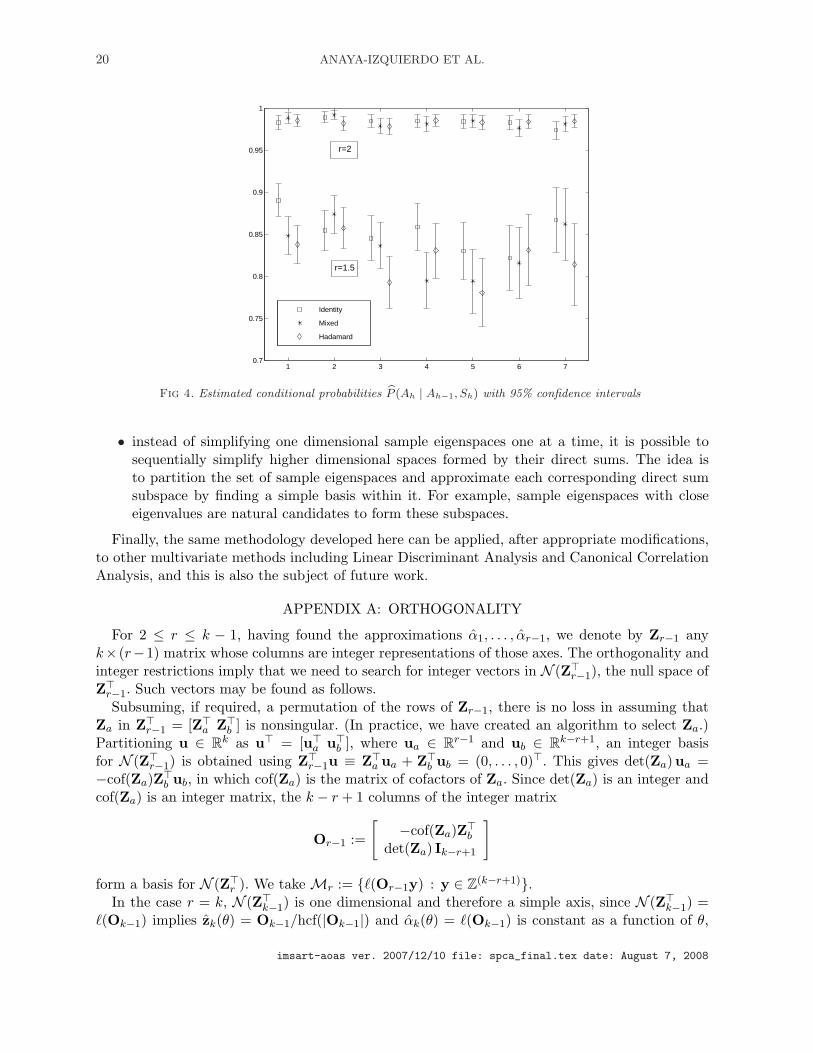
population eigenvector given that the first (h − 1) population eigenspaces have been exactlyrecovered and the first h sample eigenvectors appeared in the same order as their populationcounterparts, for h = 1, . . . , k. By orthogonality, P (Ak | Ak−1, Sk) = 1. The estimated conditionalprobabilities P (Ah | Ah−1, Sh) for h < k are shown in Figure 4.

These probabilities are very large, which is a surprising result given that the number of possiblesimple orthogonal matrices of dimension k×k with complexities no larger than N is of order Nk2

.With r = 1.5, except for the first eigenvector, all three eigenstructures are equally easy to recover,at around 80% or better. When r = 2, the recovery is essentially identical – and well over 95% –for all three structures. A more detailed simulation study appears in a separate paper.

5. Discussion. This paper provides a methodology to systematically find a family of integerorthogonal matrices, each of whose members approximate the matrix of eigenvectors of a givencovariance or correlation matrix, amongst which the scientist or expert in the field can choose themost interpretable ones. Each approximate eigenvector is constructed to be close in angle to itsexact counterpart, while keeping the size of its maximum element as low as possible.

We showed by example that the approximations obtained are useful in practice, and by sim-ulation that the method can have very good theoretical properties such as recovering simplepopulation structure exactly, when such exists. The exploratory nature of the method, as com-pared to other similar methods, offers more possibilities for interpretation, while not compromisingthe usefulness of certain modelling assumptions like groups or contrasts. It is also shown that themethod performs well with respect to other simplification methods that produce integer vectors.

Variations of our methodology for future study include:

• varying the minimum accuracy required across axes• using other orders of computation, apart from the four considered in this paper, to explore

more extensively the vast space of integer orthogonal matrices• in the complete case k′ = k each approximation is a rotation, so we can explore more deeply

the relation with other well-known rotation techniques



1 2 3 4 5 6 70.7

0.75

0.8

0.85

0.9

0.95

1

r=1.5

r=2

Identity

Mixed

Hadamard

Fig 4. Estimated conditional probabilities P (Ah | Ah−1, Sh) with 95% confidence intervals

• instead of simplifying one dimensional sample eigenspaces one at a time, it is possible tosequentially simplify higher dimensional spaces formed by their direct sums. The idea isto partition the set of sample eigenspaces and approximate each corresponding direct sumsubspace by finding a simple basis within it. For example, sample eigenspaces with closeeigenvalues are natural candidates to form these subspaces.

Finally, the same methodology developed here can be applied, after appropriate modifications,to other multivariate methods including Linear Discriminant Analysis and Canonical CorrelationAnalysis, and this is also the subject of future work.

APPENDIX A: ORTHOGONALITY

For 2 ≤ r ≤ k − 1, having found the approximations α1, . . . , αr−1, we denote by Zr−1 anyk× (r−1) matrix whose columns are integer representations of those axes. The orthogonality andinteger restrictions imply that we need to search for integer vectors in N (Z>r−1), the null space ofZ>r−1. Such vectors may be found as follows.

Subsuming, if required, a permutation of the rows of Zr−1, there is no loss in assuming thatZa in Z>r−1 = [Z>a Z>b ] is nonsingular. (In practice, we have created an algorithm to select Za.)Partitioning u ∈ Rk as u> = [u>a u>b ], where ua ∈ Rr−1 and ub ∈ Rk−r+1, an integer basisfor N (Z>r−1) is obtained using Z>r−1u ≡ Z>a ua + Z>b ub = (0, . . . , 0)>. This gives det(Za)ua =−cof(Za)Z>b ub, in which cof(Za) is the matrix of cofactors of Za. Since det(Za) is an integer andcof(Za) is an integer matrix, the k − r + 1 columns of the integer matrix

Or−1 :=

[−cof(Za)Z>b

det(Za) Ik−r+1

]

form a basis for N (Z>r ). We take Mr := {`(Or−1y) : y ∈ Z(k−r+1)}.In the case r = k, N (Z>k−1) is one dimensional and therefore a simple axis, since N (Z>k−1) =

`(Ok−1) implies zk(θ) = Ok−1/hcf(|Ok−1|) and αk(θ) = `(Ok−1) is constant as a function of θ,



(hcf(|u|) denoting again the highest common factor of the absolute values of the nonzero entriesof u).

APPENDIX B: IMPLEMENTATION

Numerically, we do not necessarily obtain exactly the best simple θ approximation to αr or-thogonal to α1, . . . , αr−1. Instead, we compute the following approximations. We restrict attentionto axes generated by vectors of the form Or−1y with Or−1 a k × (k − r + 1) orthogonal matrixand y ∈ Z(k−r+1) (see Section 2.2). We obtain an approximation αr(θ) to αr(θ) as follows:

1. Obtain a set of candidate vectors Y for y.2. Obtain `(Or−1Y) which is the set of axes generated by vectors in Or−1Y (the image of Y

under the linear mapping Or−1) and find the minimum complexity Nr(θ) of the axes in`(Or−1Y).

3. αr(θ) is given by the most accurate vector of the axes in `(Or−1Y) with complexity Nr(θ).

To obtain Y we focus attention on y∗ := (O>r−1Or−1)−1O>

r−1qr (note that Or−1y∗ = q⊥r ). Fora user-chosen Nmax ≥ 1, we put Y := ∪N≤NmaxYN where, for each N ≤ Nmax, YN is constructed,as detailed below, with a set of candidate vectors in Z(k−r+1) used to minimise the angle with y∗.There is no loss in reversing the signs of any negative entries in y∗ and then placing its entriesin non-increasing order, (the corresponding inverse permutation and sign changes being appliedto all candidate vectors to recover the original signs and order). We compute first the number ofiterations

IN =min{N,k−r}+1∑

i=1

(k − r − 1

i− 1

)(N + 1

i

)

required for an exhaustive search for fixed N and compare this with a user-chosen limit Imax. IfIN ≤ Imax, we take YN as the set of all non-increasing nonnegative integer vectors with complexityN . If IN > Imax we start with the vector (N, 0, . . . , 0), then look over all (N, i, 0, . . . , 0) fori = 0, . . . , N and keep the one which minimises the angle with y. If the minimum is attained atzero then stop, otherwise proceed in the same way for the next entry. YN is the set all vectorsencountered in this process. The case r = 1 is covered for the first approximation by taking Or−1

as the identity matrix.Experience has shown that values of Nmax = 9 and IN = 20, 000 give accurate results, while

keeping the computations fast, and that the algorithm appears to be stable so long as the integerentries do not become huge. Details of the calculations appear in the corresponding R routinesimplify.r which is available from the authors upon request.

ACKNOWLEDGEMENTS

We are grateful to Paddy Farrington and Chris Jones for useful comments on earlier versionsof this manuscript, and to Nickolay Trendafilov for helpful discussions.

REFERENCES

[1] Cadima, J. and Jolliffe, I. T.(1995). Loadings and correlations in the interpretation of principal components.Journal of Applied Statistics 22(2) 203–241.

[2] Chipman, H. A. and Gu, H.(2005). Interpretable dimension reduction. Journal of Applied Statistics 32(9)969–987.

[3] D’Aspremont, A. and El Ghaoui, L. and Jordan, M. I. and Lanckriet, G. R. G.(2007). A directformulation for sparse PCA using semidefinite programming. SIAM Review 49(3) 434–448.



[4] Fang, K.and Li, R.(1997). Some methods for generating both an NT-net and the uniform distribution on aStiefel manifold and their applications. Computational Statistics & Data Analysis 24 29–46.

[5] Farcomeni, A.(2008). An exact approach to sparse principal component analysis. Computational Statistics, toappear.

[6] Hausman, R. E.(1982). Constrained Multivariate Analysis. Studies in the Managment Sciences 19 137–151.[7] Jeffers, J.N.R.(1967). Two case studies in the application of principal component analysis. Applied Statistics

16 225–236.[8] Jolliffe, I. T. (2002). Principal Component Analysis. Springer-Verlag New York, Inc.[9] Jolliffe, I. T. and Trendafilov, N. T. and Uddin, M.(2003). A Modified Principal Component Technique

Based on the LASSO. Journal of Computational and Graphical Statistics 12(3) 531–547.[10] Mardia, K. V. and Kent, J. T. and Bibby, J. M. (1979). Multivariate Analysis. Academic Press.[11] Moghaddam, B. and Weiss, Y. and Avidan, S.(2006). Spectral bounds for sparse PCA: exact and greedy

algorithms. Advances in Neural Information Processing Systems. 18 915–922.[12] Park, T.(2005). A penalized likelihood approach to rotation of principal components. Journal of computational

and graphical statistics 14(4) 867–888.[13] Rousson, V. and Gasser, T.(2003). Some case studies of simple component analysis. Unpublished

manuscript.[14] Rousson, V. and Gasser, T.(2004). Simple component analysis. Applied Statistics 53(4) 539–555.[15] Sjostrand, K. and Stegmann, M. B. and Larsen, R.(2006). Sparse principal component analysis in medical

shape modeling. International Symposium on Medical Imaging 2006. 1579-1590.[16] Sun, L. (2006). Simple Principal Components. Ph.D. Thesis. The Open University.[17] Thompson, M.O. and Vines, S.K. and Harrington, K. (1999). Assessment of blood volume flow in the

uterine artery: the influence of arterial distensibility and waveform abnormality. Ultrasound in Obstetrics andGynecology 14(1) 71.

[18] Trendafilov, N. T. and Jolliffe, I. T.(2007). dalass: Variable selection in discriminant analysis via theLASSO. Computational Statistics and Data Analysis 51(8) 3718–3736.

[19] Vines, S. K.(2000). Simple principal components. Applied Statistics 49(4) 441–451.[20] Zou, H. and Hastie, T. and Tibshirani, R. (2006). Sparse principal component analysis. Journal of Com-

putational and Graphical Statistics 15(2) 265–286.

Department of Mathematics and Statistics, The Open University,Walton Hall, Milton Keynes, MK7 6AA, United KingdomE-mail: [email protected]


Documents

ORTHOGONAL SIMPLE COMPONENT ANALYSISstats- · ORTHOGONAL SIMPLE COMPONENT ANALYSIS By Karim Anaya-Izquierdo, ... Again, exact zeros and simple averages appear natu-rally