Orthogonal Representationsof Finite Groups

Dissertation

Oliver Braun

October 9, 2016

2

Updated version

This is an updated version of my PhD thesis. An error in Remark 6.5.9 is corrected andin Section 6.4 I include a reference to [BN16], which removes the restriction that n be 1or 2.

Oliver BraunOctober 9, 2016

3

4

Contents

1 Introduction 7

2 Symbols, notations and conventions 11

3 Bilinear and quadratic forms 123.1 First definitions . . . . . . . . . . . . . . . . . . . . . . . . . . . . . . . . . 123.2 Orthogonal groups and Witt’s theorem . . . . . . . . . . . . . . . . . . . . 193.3 The Witt group . . . . . . . . . . . . . . . . . . . . . . . . . . . . . . . . . 213.4 Quadratic forms over certain rings . . . . . . . . . . . . . . . . . . . . . . 223.5 Lattices . . . . . . . . . . . . . . . . . . . . . . . . . . . . . . . . . . . . . 263.6 Clifford algebras . . . . . . . . . . . . . . . . . . . . . . . . . . . . . . . . 27

4 Orthogonal representations 364.1 Representation theory . . . . . . . . . . . . . . . . . . . . . . . . . . . . . 364.2 Orthogonal representations . . . . . . . . . . . . . . . . . . . . . . . . . . 424.3 Various methods . . . . . . . . . . . . . . . . . . . . . . . . . . . . . . . . 48

4.3.1 Restriction . . . . . . . . . . . . . . . . . . . . . . . . . . . . . . . 484.3.2 Permutation representations . . . . . . . . . . . . . . . . . . . . . . 484.3.3 Tensor products and exterior and symmetric powers . . . . . . . . 484.3.4 Trace forms of Hermitian forms . . . . . . . . . . . . . . . . . . . . 504.3.5 Orthogonal Frobenius Reciprocity . . . . . . . . . . . . . . . . . . 504.3.6 A Clifford theory of orthogonal representations . . . . . . . . . . . 524.3.7 Nebe’s character method . . . . . . . . . . . . . . . . . . . . . . . 54

5 Representations of Schur index 2 595.1 Totally real fields . . . . . . . . . . . . . . . . . . . . . . . . . . . . . . . . 595.2 Finite fields . . . . . . . . . . . . . . . . . . . . . . . . . . . . . . . . . . . 61

6 Orthogonal representations of certain infinite families of finite groups 656.1 Symmetric groups . . . . . . . . . . . . . . . . . . . . . . . . . . . . . . . 656.2 Cyclic groups . . . . . . . . . . . . . . . . . . . . . . . . . . . . . . . . . . 676.3 Semidirect products of cyclic groups . . . . . . . . . . . . . . . . . . . . . 696.4 SL2(q) . . . . . . . . . . . . . . . . . . . . . . . . . . . . . . . . . . . . . . 716.5 SL2(2n) . . . . . . . . . . . . . . . . . . . . . . . . . . . . . . . . . . . . . 87

5

7 Clifford orders 927.1 Basic properties . . . . . . . . . . . . . . . . . . . . . . . . . . . . . . . . . 927.2 The trace bilinear form . . . . . . . . . . . . . . . . . . . . . . . . . . . . 947.3 The Jacobson radical and the idealizer . . . . . . . . . . . . . . . . . . . . 96

7.3.1 Hereditary orders and the radical idealizer process . . . . . . . . . 987.3.2 Odd residue class field characteristic . . . . . . . . . . . . . . . . . 997.3.3 Even residue class field characteristic . . . . . . . . . . . . . . . . . 103

7.4 Idempotents . . . . . . . . . . . . . . . . . . . . . . . . . . . . . . . . . . . 111

8 Algorithms and methods 1148.1 Invariant forms . . . . . . . . . . . . . . . . . . . . . . . . . . . . . . . . . 1148.2 Clifford invariants . . . . . . . . . . . . . . . . . . . . . . . . . . . . . . . 1158.3 Characters on Clifford algebras and square roots of characters . . . . . . . 1168.4 Radical idealizers . . . . . . . . . . . . . . . . . . . . . . . . . . . . . . . . 118

9 Computational results and examples 1209.1 How to read the tables . . . . . . . . . . . . . . . . . . . . . . . . . . . . . 1209.2 Atlas groups . . . . . . . . . . . . . . . . . . . . . . . . . . . . . . . . . . 123

9.2.1 A7 . . . . . . . . . . . . . . . . . . . . . . . . . . . . . . . . . . . . 1249.2.2 L3(3) . . . . . . . . . . . . . . . . . . . . . . . . . . . . . . . . . . 1259.2.3 U3(3) ∼= G2(2)′ . . . . . . . . . . . . . . . . . . . . . . . . . . . . . 1269.2.4 M11 . . . . . . . . . . . . . . . . . . . . . . . . . . . . . . . . . . . 1279.2.5 A8

∼= L4(2) . . . . . . . . . . . . . . . . . . . . . . . . . . . . . . . 1279.2.6 L3(4) . . . . . . . . . . . . . . . . . . . . . . . . . . . . . . . . . . 1289.2.7 U4(2) ∼= S4(3) . . . . . . . . . . . . . . . . . . . . . . . . . . . . . . 1309.2.8 Sz(8) . . . . . . . . . . . . . . . . . . . . . . . . . . . . . . . . . . 1319.2.9 U3(4) . . . . . . . . . . . . . . . . . . . . . . . . . . . . . . . . . . 1319.2.10 M12 . . . . . . . . . . . . . . . . . . . . . . . . . . . . . . . . . . . 1329.2.11 U3(5) . . . . . . . . . . . . . . . . . . . . . . . . . . . . . . . . . . 1339.2.12 J1 . . . . . . . . . . . . . . . . . . . . . . . . . . . . . . . . . . . . 1349.2.13 A9 . . . . . . . . . . . . . . . . . . . . . . . . . . . . . . . . . . . . 1359.2.14 O+

8 (2) . . . . . . . . . . . . . . . . . . . . . . . . . . . . . . . . . . 1369.2.15 M24 . . . . . . . . . . . . . . . . . . . . . . . . . . . . . . . . . . . 1369.2.16 M cL . . . . . . . . . . . . . . . . . . . . . . . . . . . . . . . . . . . 1379.2.17 R(27) . . . . . . . . . . . . . . . . . . . . . . . . . . . . . . . . . . 1379.2.18 S8(2) . . . . . . . . . . . . . . . . . . . . . . . . . . . . . . . . . . . 1379.2.19 Co3 . . . . . . . . . . . . . . . . . . . . . . . . . . . . . . . . . . . 137

9.3 Extensions of finite groups by finite simple groups . . . . . . . . . . . . . 1389.3.1 PΓL2(8) ∼= PΣL2(8) . . . . . . . . . . . . . . . . . . . . . . . . . . 1389.3.2 PΓL2(32) ∼= PΣL2(32) . . . . . . . . . . . . . . . . . . . . . . . . . 139

Bibliography 140

Index 143

6

1 Introduction

In ordinary representation theory of finite groups one studies linear actions of finitegroups on finite-dimensional vector spaces over a field K whose characteristic does notdivide the group order. Such an action on a vector space V naturally gives rise to anaction on K[V ], the ring of polynomial functions on V . The study of fixed points of Gon K[V ] is the subject of algebraic invariant theory, which originated in the nineteenthcentury and was later extended to include geometric aspects of orbit spaces of linearalgebraic groups on algebraic varieties and schemes.

In fact, the idea of examining properties of mathematical objects that stay the samewhen certain transformations are applied to the object is so universal that it pervadesall of mathematics. Examples include elementary geometric properties such as the sumof the angles of a triangle and the ratio of the radius and circumference of a circle,which are constant for triangles of all shapes and sizes and circles of all radii. In linearalgebra, the trace and determinant of a linear endomorphism remain unchanged whenbase change is applied, in discrete mathematics an example is provided by the chromaticnumber of a graph, which is an invariant under graph isomorphisms and in measuretheory, the famous Lebesgue measure of a set is unaffected by translations.

Returning to the subject of representation theory of finite groups, consider a represen-tation ∆ : G → GL(V ). We pose the question whether there exists a non-degeneratequadratic form q on V such that ∆(G) is a subgroup of the orthogonal group O(V, q) –justifying the designation “orthogonal representation” for such a pair (V, q). If that isthe case q is necessarily an invariant of the naturally induced action of G on the space ofall quadratic forms on V and the task of investigating the properties of q suggests itself.In fact under some mild restrictions the existence of such a quadratic form is guaranteedand the inspection of its properties is the central topic of this thesis.An alternative formulation of this problem is the following. Given ∆, assume that thespace of G-invariant quadratic forms on V is one-dimensional, in which case we call therepresentation ∆ uniform. It is well known that the so-called character χ – which isdefined as χ(g) = tr(∆(g)) for all g ∈ G – completely determines ∆ up to a suitableequivalence relation. So it is fair to say that χ determines q up to multiplication byscalars of K. Our research problem, which is precisely formulated on page 46, may nowbe stated as: How can one read off properties of q from the character χ?

We borrow suitable invariants to determine the isometry class of q from the algebraic

7

theory of quadratic forms, which was originally a branch of number theory linked todiophantine equations. It grew to become an independent subject of mathematics withdeep connections not only to number theory but also geometry, group theory, topologyand modular forms.For the present work the discriminant d±(q) and the Clifford invariant c(q), which areintroduced in due course, are of tremendous importance.

A remarkably simple answer to the abovementioned question exists in case the characterχ has values in an imaginary quadratic number field Q(

√δ). There exists no G-invariant

quadratic form on V , however χ+χ is the character of a uniform representation and thearising quadratic form q has discriminant d±(q) = δχ(1). Under favorable circumstancesone may even derive the Clifford invariant from the knowledge of δ and representation-theoretic properties of χ. See Theorem 4.3.9 for details.

The relationship between χ and the isometry type of q was also investigated by GabrieleNebe in [Neb99] and the subsequent publication [Neb00a], where a character-theoreticmethod was developed and applied to provide an answer in some cases. Another result ofNebe’s is a version of Frobenius reciprocity for orthogonal representations which yields,among other things, a description of the Sn-invariant bilinear forms on some irreduciblerepresentations. We give an account of both methods in the body of this thesis, cf.Corollary 4.3.20 and Theorem 4.3.13.

Outline and results

Chapter 3 serves as an introduction to the algebraic theory of bilinear and quadraticforms. We introduce the abovementioned invariants d± and c for quadratic forms anddiscuss quadratic forms over certain kinds of rings. While most of the covered material,which we mainly extracted from Martin Kneser’s work [Kne02], is classical and wellknown to experts, we present a useful periodicity result for the Clifford invariant whichwe have not found in the literature. It describes a periodicity modulo 8 in the sequence

c(ϕ), c(ϕk ϕ), c(ϕk ϕk ϕ), ...

for regular quadratic spaces ϕ, cf. Theorem 3.6.26.

We begin the fourth chapter by briefly introducing the necessary tools and results fromthe representation theory of finite groups. We then proceed to define orthogonal repre-sentations, give some structure results and precisely formulate the central research taskfor this thesis. The conclusion of the chapter consists of several general methods totackle the question of determining the K-isometry class of q for an orthogonal represen-tation (V, q), including the three methods mentioned above and a novel result which isa version of Clifford’s theorem for orthogonal representations of normal subgroups, cf.Theorem 4.3.14.

8

Chapter 5 briefly touches upon the subject of orthogonal representations with Schurindex 2. We outline previous work on the matter by Alexandre Turull, [Tur93], andformulate a conjecture for a similar situation.

Those general results are then applied in Chapter 6 which is devoted to orthogonalrepresentations of some infinite families of finite groups. First the work of GabrieleNebe on cyclic and symmetric groups is reviewed. Then we discuss new findings onsemidirect products of cyclic groups and present a nearly complete classification of theorthogonal representations of the finite groups SL2(q) for arbitrary prime powers q. Thedetails of this classification are the contents of Theorems 6.4.27 and 6.5.10. Clearlythese are interesting results in their own right, but they are also of considerable usewhen trying to determine the orthogonal representations of the finite simple groups.This is because the groups PSL2(q) are not only simple but also frequently appear as(maximal) subgroups of other such groups.

The following chapter is predominantly of independent interest. It is concerned withwhat we call Clifford orders, which we define as follows. Let L be an integral lattice ina quadratic space (V, q) with Clifford algebra g : V → C(V, q). Then

C(L) := 〈g(`) | ` ∈ L〉 ,

the order generated by the image of L in C(V, q), is called the Clifford order of L.We provide some basic properties of such orders before studying their p-adic Jacobsonradicals and the first step of the radical idealizer process, which is a procedure to obtain ahereditary over-order dating back at least to work of Herbert Benz and Hans Zassenhaus,[BZ85]. Our examination of the radical idealizer process culminates in a characterizationof the hereditary Clifford orders in terms of invariants of the quadratic lattice (L, q) forodd and even residue class characteristics.Finally we discuss idempotents in p-adic Clifford orders, which concludes the theoreticalpart of this thesis.

In Chapter 8 we present the algorithms used in our studies. We give pseudo-code forall algorithms so that they may be easily implemented in any suitable computer algebrasystem.

The last chapter contains a number of examples of classifications of orthogonal repre-sentations which were obtained through both the theoretical and algorithmic methodspresented in the previous chapters. We focus mainly on finite simple groups discussed inthe Atlas of Finite Groups [CCN+85] as they offer a wealth of interesting examplesand also provide us with some computational challenges due to their increasing size andcomplexity.

9

Acknowledgements

In the first place I wish to thank my advisor Prof. Dr. Gabriele Nebe. Not onlydid she suggest the interesting research topic of my thesis, she also provided me withvaluable advice countless times and always demonstrated great interest in my work. Prof.Nebe also acted as the speaker of the DFG research training group “Experimental andConstructive Algebra” from which I held a scholarship during my work on this thesis. Iam indebted to the DFG for providing me with funding and thereby the possibility topursue this research project.

It has been a privilege to work with many distinguished colleagues at Lehrstuhl D furMathematik. Above all I should mention my friend and colleague Sebastian Schonnen-beck, to whom I am grateful for numerous fruitful discussions and constant encourage-ment. Furthermore my thanks go to Dr. Markus Kirschmer for helpful advice concerningthe computer algebra system Magma.

Finally I would like to thank my friends, my parents and my siblings for supporting methroughout my studies.

10

2 Symbols, notations and conventions

Sets and combinatorics

1. The disjoint union of sets is denoted by t.2. The difference of sets is denoted by −.3. In this thesis, the set N of natural numbers does not contain 0.

We write N0 = {0} ∪N.4. If n ∈ N is a natural number, we write n := {x ∈ N | x ≤ n}.

5. For n ∈ N, we define

(n

k

):=

{n!

k!(n−k)! 0 ≤ k ≤ n,0 k < 0 or k < n.

Rings

1. All rings are associative and unital. Commutativity of multiplication is not as-sumed.

2. If R is a ring, R× denotes its unit group.3. If R is commutative, (R×)2 := {x2 | x ∈ R×} denotes the subgroup of squares ofR×.

4. Z(R) denotes the center of R, i.e. Z(R) = {x ∈ R | xy = yx for all y ∈ R}.5. If R is an integral domain, we dnote by Quot(R) the quotient field, or field of

fractions, of R.6. For n× n-matrices over a ring R, we use the notation Rn×n, or, if the expression

for n is more complicated, Matn(R).

Modules

1. Unless otherwise stated, all modules considered are left modules.2. If M is an R-module, M∗ denotes the dual R-module HomR(M,R).

Groups

1. If n is a natural number, Cn designates an abstract cyclic group of order n.

11

3 Bilinear and quadratic forms

3.1 First definitions

In this section let A denote a commutative ring. Although there is classically a strongpreference for studying quadratic forms over fields of characteristic distinct from two,we will define as many of the concepts as possible for commutative rings of arbitrarycharacteristic, mainly following Martin Kneser’s “Quadratische Formen” [Kne02], fromwhich we cite most definitions and results.

Definition 3.1.1 (Bilinear modules) Let M be a module over A and b a symmetricbilinear form on M , that is, a map

b : M ×M → A

satisfying b(x, y) = b(y, x) and b(ax + y, z) = ab(x, z) + b(y, z) for all x, y, z ∈ M anda ∈ A. Then we call (M, b) a bilinear A-module.

Definition 3.1.2 (Isometry of bilinear forms) Let (M, b), (M ′, b′) be two bilinearA-modules. An isometry (sometimes more precisely referred to as an isometric embed-ding)

ϕ : (M, b)→ (M ′, b′)

from (M, b) to (M ′, b′) is an injective A-module homomorphism with the additionalproperty that for all x, y ∈M we have b′(ϕ(x), ϕ(y)) = b(x, y).(M, b) and (M ′, b′) are said to be isometric, written as (M, b) ∼= (M ′, b′), if there is abijective isometry between them, in which case the inverse map ϕ−1 is an isometry aswell, thus yielding an equivalence relation on bilinear spaces.

Definition 3.1.3 (Orthogonality) Let (M, b) be a bilinear module over A with ele-ments x, y ∈M and a submodule N ⊆M .

1. x and y are called orthogonal (or perpendicular) if b(x, y) = 0.

2. N⊥ := {x ∈ M | b(x, f) = 0 for all f ∈ F} is called the orthogonal submodule ofN (one easily checks that this is indeed a submodule of M and that (F⊥)⊥ ⊇ F ).

12

3. Let M1, ...,Mn be submodules of M . We say that M is the orthogonal direct sumof the submodules M1, ...,Mn if

M =n⊕i=1

Mi

and b(Mi,Mj) = {0} for 1 ≤ i 6= j ≤ n. In this situation, we write

M =n

ë

i=1

Mi.

Definition 3.1.4 If V is an A-module, we let V ∗ := HomA(V,A).Given a submodule N of a bilinear A-module (M, b), we define the module homomor-phism

bN : M → N∗,m 7→(n 7→ b(m,n)

).

Notice that ker(bN ) = N⊥.

Lemma 3.1.5 ([Kne02, (1.3)]) Again, let (M, b) be a bilinear module with submoduleN . We have M = N kN⊥ if and only if N ∩N⊥ = {0} and bN (M) = bN (N).

Definition 3.1.6 A bilinear module (M, b) is called non-degenerate if bM is injective,i.e. M⊥ = {0}. The bilinear module is called regular if bM is injective and M is finitelygenerated and projective as an A-module.A submodule N ≤ M is called non-degenerate or regular if these properties hold for(N, b|N×N ).

Theorem 3.1.7 ([Kne02, Satz (1.6)]) Any regular submodule of a bilinear module(M, b) is an orthogonal direct summand of M .

Theorem 3.1.8 ([Kne02, Satz (1.7)]) An orthogonal direct sum of bilinear modulesis non-degenerate or regular, respectively, if and only if this holds for each summand.

If the bilinear A-module under consideration is free of finite rank as an A-module, thereis an important invariant of the isometry class, which we will now define.

Definition 3.1.9 (Gram matrix) Let (M, b) be a free bilinear A-module of finite rankn with ordered basis B := (m1, ...,mn). The matrix (b(mi,mj))1≤i,j,≤n is called theGram matrix of (M, b) with respect to the basis B.

Definition 3.1.10 We denote a free bilinear A-module with an n × n-Gram matrixG = (gi,j)1≤i,j≤n by ⟨g1,1 ... g1,n

... ......

gn,1 ... gn,n

⟩.

If G is a diagonal matrix with elements g1, ..., gn on the diagonal we also write 〈g1, ..., gn〉.

13

Notice that if we perform a base change on M , using a matrix T ∈ GLn(A), the Grammatrix G changes to T trGT . This motivates the following definition.

Definition 3.1.11 (Determinant and discriminant) Let (M, b) be a free bilinearA-module with Gram matrix G (with respect to some basis). Then we call

det(M, b) := det(G)(A×)2 ∈ A/(A×)2

the determinant of (M, b). The fact that we have defined the determinant to be anelement of the square class group A/(A×)2 renders this construction independent of thechoice of a basis, thus yielding an isometry invariant.Putting m := rankA(M), we call the invariant

d±(M, b) := (−1)m(m−1)/2 det(M, b) ∈ A/(A×)2,

which sometimes shows a more desirable behavior than det(M, b), the discriminant of(M, b).

We can now describe non-degeneracy and regularity of bilinear spaces in terms of theirdeterminants.

Theorem 3.1.12 ([Kne02, Satz (1.15)]) A free bilinear module (M, b) over a ring Ais non-degenerate if and only if det(M, b) is not a zero divisor in A. It is regular if andonly if det(M, b) is invertible.

If the ring A is a field we obtain some stronger results which we shall briefly discussnow.

Theorem 3.1.13 ([Kne02, Satz (1.19)]) A finite-dimensional bilinear space over afield is regular if and only if it is non-degenerate.For any subspace F of a regular bilinear space (V, b) we have

dim(F ) + dim(F⊥) = dim(V )

and (F⊥)⊥ = F .

Theorem 3.1.14 ([Kne02, Satz (1.20)]) Let (V, b) be a finite-dimensional bilinearspace over a field A. There is a decomposition

V =

(r

ë

i=1

Vi

)k F

where all Vi are regular subspaces of dimension 1 or 2 and b(F, F ) = 0. V is regular ifand only if F = {0}.In case the characteristic of A is not two, one may choose the Vi to be one-dimensional.A suitable basis may be found by extending a basis of F to a basis of V by choosingvectors which are pairwise orthogonal.

14

Example 3.1.15 In this example, we present two infinite series of important bilinearmodules over the ring Z.

1. Let L := Zn and

b : L× L→ Z, (x, y) 7→n∑i=1

xiyi.

Then we define In to be the bilinear Z-module (L, b). With respect to the standardbasis {e1, ..., en} of L the Gram matrix of In is the identity matrix - the determinantis det(In) = 1.In is decomposable as

Ëni=1〈1〉.

2. An := {(x1, ..., xn+1) ∈ In+1 |∑n+1

i=1 xi = 0} ≤ In+1. A Z-basis of An is given by

e1 − e2, e2 − e3, ..., en − en+1

with Gram matrix

2 −1−1 2 −1

−1 2. . .

2 −1−1 2

.

We obtain det(An) = n+ 1.Notice that An is the orthogonal module of the vector (1, 1, ..., 1) ∈ In+1.

Next, we will define quadratic forms.

Definition 3.1.16 (Quadratic forms) Let E be an A-module and consider a mapq : E → A satisfying

q(ax) = a2q(x) for all a ∈ A, x ∈ E and

q(x+ y) = q(x) + q(x) + bq(x, y)

for some bilinear form bq on E. (E, q) is called a quadratic A-module.

Definition 3.1.17 (Isometry of quadratic forms) Assume that (E, q) and (E′, q′)are two quadratic modules. An isometry f : (E, q) → (E′, q′) is a module monomor-phism E → E′ such that q′(f(x)) = q(x) for all x ∈ E.(E, q) and (E′, q′) are said to be isometric, written (E, q) ∼= (E′, q′), if there is a bijectiveisometry between them, just as in the case of bilinear modules.

Definition 3.1.18 (Scaling of modules and forms) Let ϕ := (E, f) be a bilinearor quadratic module over a ring A. Then we put aϕ := (aE, f) and a ◦ ϕ := (E, af) fora ∈ A.

15

Definition 3.1.19 (Extension of scalars) If (E, q) is a quadratic module over A andS ⊇ A is a ring extension, we define S ⊗A (E, q) to be the quadratic S-module (S ⊗AE, qS), where qS is defined by qS(s⊗ e) := s2q(e) and bqS (s⊗ e, s′ ⊗ e′) := ss′bq(e, e

′).We also define the scalar extension of bilinear spaces in accordance with this definition.

Remark 3.1.20 The class of all quadratic A-modules forms a category with (injective)isometries as morphisms. We denote this category by A-QMod.

Definition 3.1.21 Let (E, q) and (E′, q′) be quadratic modules over A.

1. The orthogonal direct sum of (E, q) and (E′, q′), denoted by (E, q) k (E′, q′), isdefined to be the module E ⊕ E′ with quadratic form q k q′ defined by

(q k q′)(x, x′) := q(x) + q(x′).

2. The tensor product of (E, q) and (E′, q′), (E, q)⊗ (E′, q′), is the module E ⊗A E′equipped with the quadratic form q ⊗ q′ defined by

(q ⊗ q′)(x⊗ x′) := 2q(x) · q′(x′) and bq⊗q′(x⊗ x′, y ⊗ y′) = bq(x, y) · bq′(x′, y′).

The introduction of the factor 2 in the definition of the tensor product may seem re-markable. It is, however, necessary, as will be explained in Remark 3.1.23.

Definition 3.1.22 1. A quadratic A-module (E, q) is called regular if (E, bq) is reg-ular. (E, q) is called non-degenerate if (E, bq) is non-degenerate.

2. x ∈ E is called singular if q(x) = 0.

3. A submodule F ≤ E is called singular if q(F ) = {0}.

4. (E, q) is called anisotropic if q(x) = 0 implies x = 0.

5. We define the determinant det(E, q) to be det(E, bq) ∈ A/(A×)2 and the discrim-inant d±(E, q) := d±(E, bq) ∈ A/(A×)2.

From the definition of quadratic forms we obtain the equation

4q(x) = q(2x) = q(x+ x) = 2q(x) + bq(x, x), (3.1)

implying2q(x) = bq(x, x)

which has important consequences for the theory.

16

Remark 3.1.23 Equation (3.1) sheds light on the factor 2 occurring in the definitionof the tensor product. Namely, we have

2(q ⊗ q′)(x⊗ x′) = bq⊗q′(x⊗ x′, x⊗ x′)= bq(x, x)bq′(x

′, x′)

= 2q(x) · 2q′(x′),

which shows that our definition is appropriate by cancelling the factor 2 (if 2 is not azero-divisor in A).

Remark 3.1.24 Let (M, b) be a bilinear module over A. Then M is a quadratic A-module with quadratic form qb given by

qb : M → A, m 7→ b(m,m).

In light of equation (3.1), notice that we have the equations

bqb = 2b and qbq = 2q.

This shows that the notions of bilinear modules and quadratic modules are equivalent if2 ∈ A×.Concretely, if we associate to a bilinear space (E, b) the quadratic space (E, 1

2qb), thenwe can reconstruct (E, b) via b 1

2qb

= b. Conversely, we associate to a quadratic space

(E, q) the bilinear space (E, 12bq) in order to be able to reconstruct (E, q) via q 1

2bq

= q.

If 2 /∈ A×, but 2 is not a zero divisor in A, q is still uniquely determined by bq.

Most generally, one can always find a (not necessarily symmetric) bilinear form a : E×E → A such that q(x) = a(x, x) if E is a free module of finite rank. In this case, wehave bq(x, y) = a(x, y) + a(y, x).If {e1, ..., en} is a basis of E, we have

q

(n∑i=1

xiei

)=

n∑i=1

q(ei)x2i +

∑1≤i<j≤n

bq(ei, ej)xixj

and we can define

a

n∑i=1

xiei,n∑j=1

yjej

:=∑

1≤i≤j≤nai,jxiyj , (3.2)

where ai,i := q(ei) and ai,j := bq(ei, ej) for i ≤ j.

Definition 3.1.25 A free quadratic A-module E defined as in the situation of equation(3.2) of the last remark is denoted by

(E, q) =

a1,1 a1,2 · · · a1,n

a2,2

. . .

an,n

17

or (E, q) = [a1, ..., an] if q (∑n

i=1 xiei) =∑n

i=1 aix2i .

If 2 ∈ A is not a zero divisor, we put bi,j := bq(ei, ej) = bj,i and may also write

(E, q) =

⟨b1,1 · · · b1,n... · · ·

...bn,1 · · · bn,n

⟩.

For example, letting A be a ring where 2 is not a zero divisor, if E = A is free ofrank one with basis vector e1 and quadratic form q defined by q(e1) = 1, we have(E, q) = [1] = 〈2〉.

Definition 3.1.26 (Hyperbolic modules) The free quadratic A-module (A2, q) with

q

((x1

x2

)):= x1x2 is called the hyperbolic plane over A. We denote this quadratic

module by H := H(A) and we have

H =

[0 1

0

]=

⟨0 11 0

⟩.

Notice that det(H) = −1, whence H is always a regular quadratic module over any ring.

Let (E, q) be a quadratic A-module which is finitely generated and projective. We defineH(E, q) to be a quadratic space on E ⊕ E∗ with quadratic form defined by

q(x, f) := q(x) + f(x)

for all x ∈ E and f ∈ E∗.H(E, q) is regular since as one readily verifies from the concrete description of bH(E,q) as

bH(E,q) : H(E, q)→ H(E, q)∗, (x, f) 7→(

(y, g) 7→ bq(x, y) + f(y) + g(x)).

In fact, the isometry type of the quadratic module H(E, q) is independent of q. Anisometry H(E, q) ∼= H(E, 0) is easily constructed, cf. [Kne02, (2.20)]. The quadraticspace H(E) := H(E, 0) is called the hyperbolic module associated to E.

In the case 2 /∈ A×, or even char(A) = 2, it follows from equation 3.1 that there are nofree regular quadratic modules of rank 1. In fact, there are no free regular modules ofany odd rank n, as we shall see in the following.

Theorem 3.1.27 ([Kne02, (2.9)-(2.11)]) Let (E, q) be a free quadratic A-module ofodd rank n, with basis {e1, ..., en}. Then there is a polynomial Pn ∈ Z[X1, ..., Xn(n+1)

2

]

satisfyingdet(E, q) = 2Pn(q(ei), bq(ei, ej)).

18

Definition 3.1.28 Let (E, q) be free of odd rank n and basis {e1, ..., en}. Then we call

d 12(E, q) := Pn(q(ei), bq(ei, ej))(A

×)2 ∈ A/(A×)2

the semi-determinant of (E, q). We call (E, q) semi-regular if any (and thereby all)representatives of the square class of d 1

2(E, q) are invertible in A.

Notice that we have det(E, q) = 2d 12(E, q).

Clearly our definition of the semi-determinant is independent of the choice of a basissince we have defined it to be a square class, like the determinant. If 2 ∈ A× then anysemi-regular space is also regular. In contrast, if 2 /∈ A× we can consider the quadraticmodule [1] which is not regular - it has determinant 2 - but semi-regular, as its semi-determinant is 1.

Finally we formulate an analogue of Theorem 3.1.14 for quadratic spaces over fields.

Theorem 3.1.29 ([Kne02, Satz (2.15)]) Let (E, q) be a finite-dimensional quadraticvector space over a field A. There is a decomposition

(E, q) =r

ë

i=1

Ei k

së

j=1

Fj kG

where the Ei are regular of dimension two, the Fj are semi-regular of dimension one andq(G) = {0}.

If char(A) 6= 2 we may choose r = 0 and all Fj are regular.If A is of even characteristic A2 := {a2 | a ∈ A} is a subfield of A and we may chooses ≤ [A : A2].

(E, q) is regular if and only if s = 0 and G = {0}.(E, q) is semi-regular if and only if s ≤ 1 and G = {0}.

3.2 Orthogonal groups and Witt’s theorem

Definition 3.2.1 (Orthogonal group) The automorphism group of a quadratic mod-ule (E, q) over a ring A is called the orthogonal group of (E, q). It is the group ofinvertible isometries E → E, in symbols

O(E, q) := {f : E → E | f ∈ AutA(E) and q(f(x)) = q(x) for all x ∈ E}.

If A is a field of characteristic distinct from two, we can formulate two equivalent theo-rems attributed to Witt which have far-reaching consequences.

19

Theorem 3.2.2 (Witt’s cancellation theorem) Let A be a field of characteristic nottwo and F , G1 and G2 quadratic spaces over A with F regular and F k G1

∼= F k G2.Then G1

∼= G2.

Theorem 3.2.3 (Witt’s extension theorem) Let E be a quadratic space over a fieldA with char(A) 6= 2. Let F1, F2 be regular subspaces and t : F1 → F2 a bijectiveisometry. Then there is an extension of t to E, i.e. an element u ∈ O(E) satisfyingu|F1 = t.

A proof of the equivalence of the two theorems and a proof of the statement itself maybe found in [Kne02, Satz (3.1)].

In order to formulate a generalization of this theorem which drops the hypothesis on thecharacteristic of A, we first need a definition.

Definition 3.2.4 (Primitivity) Let E be an A-module.

1. A submodule F ≤ E is called primitive if F is a direct summand of E.

2. If E carries a bilinear form b and F ≤ E is a submodule, then F is called sharplyprimitive, if it is finitely generated, projective and bF (E) = F ∗.

Remark 3.2.5 1. Any regular submodule F is sharply primitive.

2. Any sharply primitive submodule is primitive.

3. If E is regular and F ≤ E is primitive, F is sharply primitive.

Given this definition, we can now state the generalized version of Theorem 3.2.3

Theorem 3.2.6 ([Kne02, Satz (3.4)]) Let E be a quadratic space over a field A,F1, F2 ≤ E sharply primitive subspaces and t : F1 → F2 a bijective isometry. Then tmay be extended to an isometric automorphism of E.

Corollary 3.2.7 (Witt cancellation) Let F,G1 and G2 be quadratic spaces over afield A and let F be regular. Then F kG1

∼= F kG2 if and only if G1∼= G2.

Definition 3.2.8 (Witt index) If A is a field and (E, q) a finite-dimensional quadraticspace over A, the dimension of a maximal singular and sharply primitive subspace iscalled the Witt index of (E, q), denoted by ind(E, q).

Corollary 3.2.9 Let (E, q) be a quadratic space over a field A and put m := ind(E, q).Then there is a subspace F ≤ E such that ind(F, q|F ) = 0 and (E, q) ∼= (F, q|F )kH(Am).

20

Definition 3.2.10 In the situation of Corollary 3.2.9, we call (F, q|F ) the anisotropickernel of (E, q).

Definition 3.2.11 (Reflections) Let (E, q) be a quadratic A-module and e ∈ E suchthat q(e) ∈ A×. Then

se : E → E, x 7→ x− bq(x, e)q(e)−1e

is called the reflection along e.

Remark 3.2.12 Reflections se have the following properties.

1. s2e = idE .

2. se(e) = −e, se(v) = v if bq(e, v) = 0.

3. se ∈ O(E, q).

4. For any g ∈ O(E, q), we have gseg−1 = sg(e).

The following result is a consequence of Witt’s theorems.

Theorem 3.2.13 ([Kne02, Satz (3.5)]) If the quadratic space (E, q) is regular orsemi-regular over a field A, any isometric automorphism u ∈ O(E, q) may be written as

a product of reflections, unless A = F2 and E ∼=[1 1

1

]k

[1 1

1

].

3.3 The Witt group

In this section we define the Witt group of a ring. This is an Abelian group consisting ofclasses of regular quadratic forms under a certain equivalence relation which captures the“essential part” of a quadratic form. The group-theoretic structure of the Witt groupthen gives insight into the interplay of all regular quadratic forms over A.

Definition 3.3.1 Let ϕ and ψ be quadratic modules over a ring A. We call ϕ and ψWitt equivalent if there are hyperbolic modules H1 and H2 such that

ϕkH1∼= ψ kH2.

LetW (A) := {[ϕ] | ϕ is a regular quadratic A-module}

denote the set of Witt equivalence classes of regular quadratic modules over A.W (A) is an Abelian group with group law [ϕ] + [ψ] := [ϕ k ψ], −[ϕ] = [(−1) ◦ ϕ] andneutral element 0 = [H].

21

Remark 3.3.2 Clearly, if A is an integral domain, two regular quadratic modules overA are isometric if and only if they are Witt equivalent and of equal rank.

Remark 3.3.3 If A is a field, using Witt’s cancellation theorem 3.2.7 and the decom-position from Corollary 3.2.9, one obtains that two regular quadratic forms over A areWitt equivalent if and only if their anisotropic kernels are isometric.In other words, any Witt equivalence class is represented by an anisotropic space.

Example 3.3.4 If A is an algebraically closed field, we have

W (A) ∼=

{C2 char(A) 6= 2,

0 char(A) = 2.

If A = R, then any regular quadratic space ϕ may be written as

ϕ ∼=r

ë

i=1

[1] k

së

j=1

[−1]

(this result is known as Sylvester’s inertia theorem) and the map

sgn : W (R)→ Z, [ϕ] 7→ r − s,

the signature, is a group isomorphism.

We will present further examples of Witt groups in the next section.

3.4 Quadratic forms over certain rings

This section is a brief survey of quadratic forms over certain types of rings.

Finite fields

Let p ∈ Z be a prime and A ∼= Fpn a finite field.

Definition 3.4.1 (Norm form) Let E := Fp2n and let q : E → Fpn be the normform, that is, q(x) = x · xpn , which is a quadratic form over Fpn with bq(x, y) =trFp2n/Fpn (xyp

n).

(E, q) is anisotropic. We call (E, q) the norm form of A and write N(A) := (E, q).

22

Remark 3.4.2 (Quadratic spaces of dimension one and two) We have

[A× : (A×)2] =

{2 p 6= 2,

1 p = 2,

which shows that there are only one or two (semi-)regular spaces over a finite field,depending on the characteristic.Any regular quadratic space of dimension two is isometric to either H(A) or N(A), cf.[Kne02, (12.2)].

The following classification follows from Theorem 3.1.29.

Theorem 3.4.3 If ϕ is a regular quadratic A-module of dimension 2m, we have

ϕ ∼=

Ëm

i=1H∼=

Ëmi=1

[0 1

0

]or

N(A) kËm−1

i=1 H ∼=

[1 a

b

]k

Ëm−1i=1

[0 1

0

],

where X2 + aX + b ∈ A[X] is irreducible. Clearly, these two modules are not isometric.

If ϕ is semi-regular of dimension 2m+ 1, we have

ϕ ∼=

[1] k

Ëmi=1H

∼= [1] kËm

i=1

[0 1

0

]or

[ε] kËm

i=1H∼= [ε] k

Ëmi=1

[0 1

0

],

where the second case only occurs if p 6= 2 (and ε ∈ A× − (A×)2). If that happens thesetwo modules are not isometric.

Corollary 3.4.4 (Witt groups of finite fields) Put q := pn. Then we have

W (Fq) ∼=

C2 q ≡ 0 (mod 2),

C2 × C2 q ≡ 1 (mod 4),

C4 q ≡ 3 (mod 4).

For the reader’s convenience, we include the group tables for the odd characteristic cases.Notice that in these cases, the parity of the dimension and the determinant are sufficientin order to determine the isometry class of a regular quadratic Fq-space.

q ≡ 1 (mod 4), W (Fq) ∼= C2 × C2, ε ∈ F×q − (F×q )2.

23

+ [H][[1]] [

[ε]]

[N ] =[[1, ε]

][H] [H]

[[1]] [

[ε]]

[N ][[1]] [

[1]]

[H] [N ][[ε]][

[ε]] [

[ε]]

[N ] [H][[1]]

[N ] [N ][[ε]] [

[1]]

[H]

dim (mod 2) 0 1 1 0

det 1 1 ε ε

q ≡ 3 (mod 4), W (Fq) ∼= C4.

+[[1]]

[N ][[−1]

][H][

[1]]

[N ][[−1]

][H]

[[1]]

[N ][[−1]

][H]

[[1]]

[N ][[−1]

][H]

[[1]]

[N ][[−1]

][H]

[[1]]

[N ][[−1]

][H]

dim (mod 2) 1 0 1 0

det 1 1 −1 −1

Complete discretely valuated rings and fields

Let R be a complete discrete valuation ring, K = Quot(R) and k = R/πR the residuefield. We will assume that k is finite.

The ability to lift isometries, cf. Theorems (15.5) and (15.6) of [Kne02], strongly relatesproperties of quadratic forms over R with those of forms over k. Concretely, we havethe following results.

Theorem 3.4.5 There is a group isomorphism W (R) ∼= W (k).

Theorem 3.4.6 Let ϕ be a regular or semi-regular quadratic module over R. Put n :=rankR(ϕ).

1. If n is at least 3, there exists a regular or semi-regular space ψ satisfying ϕ ∼= Hkψ.

2. There are exactly two isometry types of regular R-modules of rank two, namelyH(R) and N(R) which is defined by N(R) = N(k).

3. If char(k) is odd, then ϕ ∼=Ën

i=1[1] or ϕ ∼= [ε]kËn−1

i=1 [1] for some ε ∈ R×−(R×)2.

24

4. If char(k) is even, we have the possibilities

ϕ ∼=

[1] k

Ëmi=1H(R) n = 2m+ 1,

Ëmi=1H(R) n = 2m,

N(R) kËm−1

i=1 H(R) n = 2m.

Definition 3.4.7 We put U :=(K ⊗ N(R)

)k(π ◦ (K ⊗ N(R))

). U is an anisotropic

space of dimension 4.

Theorem 3.4.8 ([Kne02, (16.3), (16.4)]) Let ϕ be regular or semi-regular over Kand ind(ϕ) = 0. Then dim(ϕ) ≤ 4 and if dim(ϕ) = 4 we have ϕ ∼= U .

We now turn our attention towards the simplest cases, namely Zp and Qp. Since one-dimensional spaces are classified by square classes, we provide the following result.

Remark 3.4.9 Let ε ∈ Z×p − (Z×p )2.

Z×p /(Z×p )2 is represented by

{{1, ε} if p 6= 2,

{1, 3, 5, 7} if p = 2.

Q×p /(Q×p )2 is represented by

{{1, ε, p, pε} if p 6= 2,

{1, 3, 5, 7, 2, 6, 10, 14} if p = 2.

Theorem 3.4.10 (W (Qp), [Kne02, (18.1)], [Sch85, 6.6]) If p is odd, there is anisomorphism W (Qp) ∼= W (Fp)×W (Fp).For p = 2 we have W (Q2) ∼= C2 × C2 × C8.

Quadratic forms over Q

We will follow Section 17 of [Kne02] in order to describe the Witt group of the field ofrational numbers.

Definition 3.4.11 Define s∞ : W (Q)→W (R) via [ϕ] 7→ [R⊗ ϕ].Define s2 : W (Q)→ Z/2Z via [ϕ] 7→ v2(d±(ϕ)) + 2Z.Both s∞ and s2 are well-defined group homomorphisms.

Due to Theorem 3.1.29, W (Q) is generated by {[a] | a ∈ Z squarefree}.

Definition 3.4.12 For p odd, define sp : W (Q) → W (Fp) on the abovementionedgenerators via

[a] 7→

{[a+ pZ] p - a,[1pa+ pZ] p | a.

sp is a well-defined group homomorphism.

25

Theorem 3.4.13 ([Kne02, Satz (17.8)]) The homomorphisms s∞, s2 and sp definean isomorphism

s : W (Q)→W (R)⊕Z/2Z⊕⊕p6=2

W (Fp).

Remark 3.4.14 By [Neb99, Satz 1.3.19], two quadratic spaces ϕ, ψ over Q are isometricif and only if they have the same dimension, determinant, signature over R and equalinvariants sp for all odd primes p.

3.5 Lattices

Let R be a Dedekind domain, K := Quot(R) its field of fractions and (V, q) a regularquadratic space over K.

Definition 3.5.1 An R-submodule L of V is called a lattice if it is finitely generatedand of maximal rank in V . Equivalently one can say that L is an R-submodule of Vwhich is finitely generated and contains a K-basis of V .

Remark 3.5.2 Sometimes a lattice as defined above is referred to as a full lattice.Then the definition of a lattice is relaxed to include R-submodules of smaller rank thandimK(V ).

Definition 3.5.3 (Integral lattice) An integral lattice L in V is an R-lattice in Vsuch that q(`) ∈ R for all ` ∈ L, which implies that bq(`1, `2) ∈ R for all `1, `2 ∈ L.

Definition 3.5.4 (Dual lattice) Let L be a lattice in V . The dual of L is defined as

L# := {x ∈ V | bq(x, `) ∈ R ∀ ` ∈ L}.

L# is again a lattice in V .

Remark 3.5.5 A lattice L in V is integral if and only if L ⊆ L#, in which case L#/Lis a finitely generated Abelian group.

If R is a principal ideal domain, any R-lattice L is a free R-module. Over an arbitraryDedekind domain this may not be the case. However, one can still say the following.

Remark 3.5.6 (Pseudo-basis) There is a K-basis {e1, ..., en} of V and fractional ide-als a1, ..., an of R such that

L = a1e1 ⊕ ...⊕ anen.

We call {(ai, ei) | 1 ≤ i ≤ n} a pseudo-basis for L.

Proof. This is the content of Theorem (4.13) of [Rei75]. �

26

If we specialize K to be a complete discretely valuated field and let R be its valuationring with maximal ideal πR, we obtain the following statement about the structure of alattice L in a regular bilinear space (V, b).

Theorem 3.5.7 (Jordan decomposition) A lattice L in (V, b) may be decomposed asfollows.

L ∼=c

ë

i=a

(La, πaba)

where a ≤ c ∈ Z such that the (Li, bi) are (semi-)regular bilinear Op-lattices, which maybe zero. The invariants rankOp(La) and det(ba) ∈ F×p /(F×p )2 are uniquely determined.In the case of an integral lattice, we have a ≥ 0.

Proof. This statement is proved in [O’M73, §91c]. �

3.6 Clifford algebras

This section is devoted to an isometry invariant of tremendous importance, which isfunctorially associated to a quadratic space, namely an A-algebra called the Cliffordalgebra. Over fields this algebra gives rise to an element of the Brauer group which willbe crucial to our study of quadratic forms and orthogonal representations.

Following [Kne02], we develop as much of the theory of the Clifford algebra as possiblefor arbitrary commutative rings. For some results however, we will have to work over afield. Therefore we let A be a commutative ring and K a field.

Definition 3.6.1 Let ϕ = (E, q) be a quadratic A-module. An A-algebra C := C(ϕ)together with an A-module homomorphism g : E → C is called a Clifford algebra if

1. For all v ∈ E we have g(v)2 = q(v) · 1C and

2. for any A-algebra B and any A-module homomorphism f : V → B satisfyingf(x)2 = q(x) · 1B there exists a unique A-algebra homomorphism ϑ : C → B suchthat the following diagram commutes.

Vf

~~g

��B C

ϑoo

Theorem 3.6.2 ([Kne02, Satz (5.4)]) For any quadratic A-module ϕ there exists aClifford algebra C(ϕ) and it is unique up to isomorphism.

27

Remark 3.6.3 If A is a field, let T (E) :=∞⊕i=0

i⊗k=1

E be the tensor algebra of E and let

I(E, q) be the two-sided ideal of T (E) which is generated by v⊗ v− q(v) · 1T (E), v ∈ E.Then C(E, q) ∼= T (E)/I(E, q), which proves the existence in a much simpler way thanthe general proof provided in [Kne02].

Corollary 3.6.4 The set {g(e) | e ∈ E} generates C(ϕ) as an A-algebra. If {ei | i ∈ S}is an A-module generating set of E and S is ordered,

∞⋃`=0

{g(ei1) · ... · g(ei`) | i1 < ... < i`}

is a generating set of C(ϕ) as an A-module.

The result of Corollary 3.6.4 can be strengthened in the following way.

Theorem 3.6.5 ([Kne02, Satz (5.12)]) If E is a free A-module of rank m with basis{e1, ..., em}, the Clifford algebra C(ϕ) is a free A-module of rank 2m with basis

m⋃`=0

{g(ei1) · ... · g(ei`) | 1 ≤ i1 < ... < i` ≤ m}.

Convention 3.6.6 When performing computations in a Clifford algebra, we will oftenomit the map g. In other words, we assume E ⊆ C(E, q), provided that no confusioncan arise from this.

Remark 3.6.7 In most cases the Clifford algebra is not commutative. Let x, y ∈ E,then in C(E, q) we have

(x+ y)2 = q(x+ y) = q(x) + q(y) + bq(x, y),

which is equal to x2 + xy + yx+ y2. We obtain

xy = −yx+ bq(x, y).

Example 3.6.8 1. Consider the free rank-one quadratic module (E, q) = [a]. ThenT (E) ∼= K[X] and therefore the Clifford algebra is isomorphic to

C(E, q) ∼= K[X]/(X2 − a).

2. If the quadratic form q on E is the zero form C(E, q) is isomorphic to the exterioralgebra

∧E.

28

Remark 3.6.9 Let A-Alg be the category of associative A-algebras with A-algebra ho-momorphisms as morphisms between the objects.

Now consider (Ei, qi) ∈ A-QMod, 1 ≤ i ≤ 3 and morphisms Eifi−→ Ei+1, i = 1, 2, which

are isometric embeddings by the definition of the category A-QMod. For 1 ≤ i ≤ 3 letEi

gi−→ C(Ei, qi) be the respective Clifford algebras. Then g2 ◦ f1 is a homomorphism ofA-modules satisfying

(g2 ◦ f1)(x)2 = q2(f1(x)) · 1C(E2,q2) = q1(x) · 1C(E2,q2).

Therefore by the universal property of C(E1, q1) there is a unique A-algebra homomor-phism C(E1, q1)→ C(E2, q2) which we denote by C(f1).C(f2) : C(E2, q2)→ C(E3, q3) may be constructed analogously.It is straightforward to see that the uniqueness property of gi forces C(id(E1,q1)) =idC(E1,q1) and C(f2 ◦ f1) = C(f2) ◦ C(f1).Therefore C is a covariant functor from A-QMod to A-Alg.

Lemma 3.6.10 If S ⊇ A is a ring extension and ϕ = (E, q) a quadratic A-module, wehave

C(S ⊗A ϕ) ∼= S ⊗A C(ϕ)

as S-algebras.

Proof. This is an application of the universal property of C(S⊗A ϕ). Let g : ϕ→ C(ϕ)be the Clifford algebra of ϕ and define g′ : S ⊗A ϕ→ S ⊗A C(ϕ) by s⊗ x 7→ s⊗ g(x).It is then easily checked that g′(s⊗ x) = qS(s⊗ x) · 1S⊗AC(ϕ).In order to prove that S ⊗A C(ϕ) also fulfills the second part of the universal propertyof C(S⊗A ϕ) let B be an S-algebra and f : S⊗AE → B an S-module homomorphismsatisfying f(s⊗ x)2 = qS(s⊗ x) · 1B.Consider ι : S → B, s 7→ s · 1B and the A-algebra homomorphism

ϑ0 : C(ϕ)→ B|A,

where B|A is the A-algebra obtained from B by restriction of scalars which is definedby the universal property of C(ϕ).Applying the universal property of the tensor product to the A-bilinear map S×C(ϕ)→B, (x, s) 7→ ι(s) · ϑ0(x) yields an A-linear map ϑ : S ⊗A C(ϕ) → B, which is alsoS-linear and multiplicative and fulfills ϑ ◦ g′ = f by construction. �

Definition 3.6.11 It follows from the proof of Theorem 3.6.2 that C(ϕ) is Z/2Z-gradedin the following way. Again, let {ei | i ∈ S} be an A-module generating set of E and put

C0 := C0(ϕ) := 〈g(ei1) · ... · g(ei2`) | ` ∈ N0, ij ∈ S〉A-Mod,

C1 := C1(ϕ) := 〈g(ei1) · ... · g(ei2`+1) | ` ∈ N0, ij ∈ S〉A-Mod.

Then, as A-modules, C(ϕ) = C0 ⊕ C1 and CiCj ⊆ Ci+j mod 2. The submodule C0 is asubalgebra of C(ϕ) called the even part of the Clifford algebra and C1(ϕ) is a C0(ϕ)-submodule of C(ϕ).For x ∈ Ci, i ∈ {0, 1}, we denote the degree of x by deg(x).

29

Definition 3.6.12 (Graded tensor product) Let A = A0⊕A1 and B = B0⊕B1 betwo Z/2Z-graded algebras. Then the graded tensor product of A and B, denoted byA ⊗ B, is A⊗B as a module with multiplication defined by

(a⊗ b)(a′ ⊗ b′) = (−1)deg(b) deg(a′)(aa′)⊗ (bb′)

for ai ∈ Ai, a′k ∈ Ak, bj ∈ Bj and b′` ∈ B`.A ⊗ B is graded via

(A ⊗ B)0 = (A0 ⊗B0)⊕ (A1 ⊗B1), (A ⊗ B)1 = (A0 ⊗B1)⊕ (A1 ⊗B0).

Theorem 3.6.13 ([Kne02, (5.10)]) If ϕ and ψ are quadratic A-modules, there is anisomorphism

C(ϕk ψ) ∼= C(ϕ) ⊗ C(ψ)

of A-algebras.

We will now focus our attention on Clifford algebras over fields in order to define theClifford invariant. Recall the definition of the Brauer group, which is presented, forexample, in [Rei75].

Definition 3.6.14 (Brauer group) Two central simpleK-algebras A and B are calledBrauer-equivalent if there are m,n ∈ N such that An×n ∼= Bm×m as K-algebras.The Brauer group Br(K) of K is defined to be the set of all Brauer equivalence classesof central simple algebras with

[A][B] := [A⊗K B], [A]−1 = [Aop], 1Br(K) = [K].

By Br2(K) we denote the maximal exponent-two subgroup of Br(K).

It turns out that, over a field, Clifford algebras of regular quadratic spaces have someadvantageous properties.

Theorem 3.6.15 ([Kne02, (11.1)-(11.2)]) Let ϕ be a regular quadratic K-space.

• If dim(ϕ) is even, C(ϕ) is a central simple K-algebra.

• If dim(ϕ) is odd, C0(ϕ) is a central simple K-algebra.The center of C(ϕ) is isomorphic to L := K[X]/(X2 − d±(ϕ)). If d±(ϕ) is not asquare in K, then L is a degree two field extension of K and C(ϕ) is a simple K-algebra with center L. Otherwise C(ϕ) is the direct sum of two isomorphic copiesof a central simple K-algebra.

In either case, C(ϕ) is a semisimple K-algebra.

30

Definition 3.6.16 (Clifford invariant) We write

c(ϕ) :=

{C(ϕ) dim(ϕ) is even,

C0(ϕ) dim(ϕ) is odd.

This is a central simple K-algebra for regular ϕ and we can therefore define

c(ϕ) := [c(ϕ)] ∈ Br(K),

the Clifford invariant of ϕ.

Remark 3.6.17 Assume that K is a field of characteristic different from two. Then itfollows from [Sch85, Lemmas 9.2.8, 9.2.9] that c(ϕ) is a tensor product of quaternion al-gebras. Therefore we actually have c(ϕ) ∈ Br2(K), the maximal exponent two subgroupof the Brauer group.If K is a number field or a p-adic field, a tensor product of quaternion algebras is Brauer-equivalent to a quaternion algebra, cf. [Vig80, I Thm. 2.9].See loc.cit. for the statement that over a number field, a quaternion algebra Q is deter-mined up to isomorphism by the even (and finite) number of places of K ramified in it,where a place p is called ramified in Q if [Kp ⊗K Q] 6= [Kp] ∈ Br(Kp). Therefore wesometimes use the notation Qp1,...,ps to denote a Quaternion algebra ramified preciselyat the places p1, ..., ps.

Theorem 3.6.18 (Product formula, [Kne02, (18.5)]) Let K be a number field, pa finite or real place of K and ϕ a regular quadratic space. Then cp(ϕ) := c(Kp⊗K ϕ) ∈Br2(Kp), and Br2(Kp) may be identified with {±1}. We then have∏

p

cp(ϕ) = 1,

where the product is taken over all finite and real places of K.

Remark 3.6.19 Due to the existence of a local-global principle for Brauer-equivalenceof central simple algebras – this is the theorem of Albert, Brauer, Hasse and Noether,cf. [Rei75, Thm. (32.11)] – over a number field K, c(ϕ) is completely determined by alllocal Clifford invariants cp(ϕ).

For explicit computations of Clifford invariants in Br2(K), it is useful to define quaternionsymbols, which generate the group Br2(K).

Definition 3.6.20 (Quaternion symbol) Let char(K) 6= 2 and a, b ∈ K×. Then(a, b) ∈ Br2(K) is defined as c([a, b]). It is the Brauer class of the quaternion algebra(a,bK

)- this notation designates the quotient of the free associative algebra on the symbols

{i, j} subject to the relations generated by i2 = a, j2 = b and ij = −ji.Commonly, one puts k := ij.

31

Lemma 3.6.21 ([Sch85, (11.8)]) Over a field of characteristic not two,(a,bK

)is a

skew field if and only if the quadratic form [1,−a,−b, ab] is anisotropic.

Remark 3.6.22 ([Vig80, Cor. II 1.2]) Let a, b, c, u, v ∈ K×. The quaternion sym-bols have the following properties.

1. (a, b) = (b, a),2. (au2, bv2) = (a, b),3. (a,−ab) = (a, b),4. (a, a) = (−1, a) = (a,−1),5. (a,−a) = [K],6. (a, bc) = (a, b)(a, c),7. (1, a) = (a, 1) = [K].

Recall that over a field of characteristic not two, any quadratic form may be diagonalized.Using this, one obtains the following result which allows for an explicit computation ofthe Clifford invariant.

Theorem 3.6.23 ([Kne02, (11.12)]) Let a1, ..., an ∈ K×, n = 2m even, r := m − 1

and s := m(m−1)2 . Then

1. c([a1, ..., an]) =∏

1≤j<i≤n(aj , ai)

(−1,

n∏i=1

ai

)r(−1,−1)s,

2. c([a1, ..., an−1]) =∏

1≤j<i≤n−1

(aj , ai)

(−1,

n−1∏i=1

ai

)r(−1,−1)s.

Proposition 3.6.24 Let ϕ and ψ be regular quadratic spaces over K, char(K) 6= 2 anda ∈ K×. Then the Clifford invariant adheres to the following rules.

1. c(a ◦ ϕ) =

{c(ϕ) · (d±(ϕ), a) dim(ϕ) even,

c(ϕ) dim(ϕ) odd.

2. If dim(ϕ) ≡ dim(ψ) mod 2,

c(ϕk ψ) = c(ϕ)c(ψ)(d±(ϕ),d±(ψ)).

3. If dim(ϕ) ≡ 1 mod 2 and dim(ψ) ≡ 0 mod 2,

c(ϕk ψ) = c(ϕ)c(ψ)(−d±(ϕ), d±(ψ)).

32

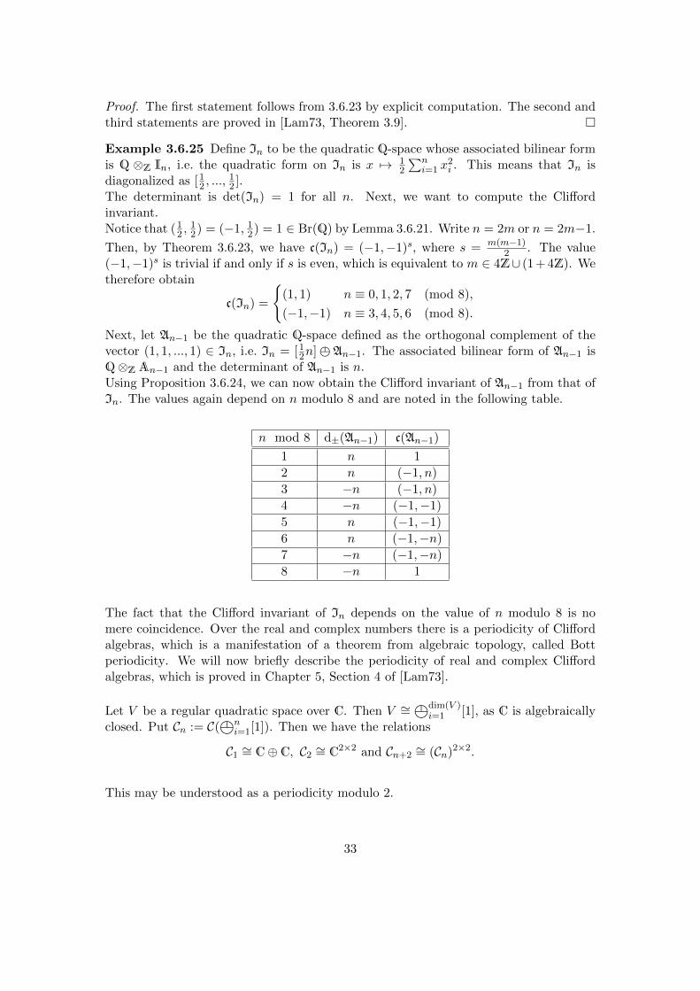
Proof. The first statement follows from 3.6.23 by explicit computation. The second andthird statements are proved in [Lam73, Theorem 3.9]. �

Example 3.6.25 Define In to be the quadratic Q-space whose associated bilinear formis Q ⊗Z In, i.e. the quadratic form on In is x 7→ 1

2

∑ni=1 x

2i . This means that In is

diagonalized as [12 , ...,

12 ].

The determinant is det(In) = 1 for all n. Next, we want to compute the Cliffordinvariant.Notice that (1

2 ,12) = (−1, 1

2) = 1 ∈ Br(Q) by Lemma 3.6.21. Write n = 2m or n = 2m−1.

Then, by Theorem 3.6.23, we have c(In) = (−1,−1)s, where s = m(m−1)2 . The value

(−1,−1)s is trivial if and only if s is even, which is equivalent to m ∈ 4Z∪ (1 + 4Z). Wetherefore obtain

c(In) =

{(1, 1) n ≡ 0, 1, 2, 7 (mod 8),

(−1,−1) n ≡ 3, 4, 5, 6 (mod 8).

Next, let An−1 be the quadratic Q-space defined as the orthogonal complement of thevector (1, 1, ..., 1) ∈ In, i.e. In = [1

2n] k An−1. The associated bilinear form of An−1 isQ⊗Z An−1 and the determinant of An−1 is n.Using Proposition 3.6.24, we can now obtain the Clifford invariant of An−1 from that ofIn. The values again depend on n modulo 8 and are noted in the following table.

n mod 8 d±(An−1) c(An−1)

1 n 1

2 n (−1, n)

3 −n (−1, n)

4 −n (−1,−1)

5 n (−1,−1)

6 n (−1,−n)

7 −n (−1,−n)

8 −n 1

The fact that the Clifford invariant of In depends on the value of n modulo 8 is nomere coincidence. Over the real and complex numbers there is a periodicity of Cliffordalgebras, which is a manifestation of a theorem from algebraic topology, called Bottperiodicity. We will now briefly describe the periodicity of real and complex Cliffordalgebras, which is proved in Chapter 5, Section 4 of [Lam73].

Let V be a regular quadratic space over C. Then V ∼=Ëdim(V )

i=1 [1], as C is algebraicallyclosed. Put Cn := C(

Ëni=1[1]). Then we have the relations

C1∼= C⊕ C, C2

∼= C2×2 and Cn+2∼= (Cn)2×2.

This may be understood as a periodicity modulo 2.

33

Over the reals we have the following situation. Let V be a regular quadratic R-space.By Sylvester’s Theorem V ∼=

Ëpi=1[1] k

Ëqj=1[−1]. We put Cp,q := C(V ). Then the

isomorphism type of Cp,q will only depend on the signature p − q modulo 8 and thedimension of V , which is p+ q.

This symbolic “clock” describes the Clifford algebras C0,0, ..., C7,0, where the arrows in-dicate a modification of the underlying quadratic space by orthogonal addition of theone-dimensional space [1].

Rp−q≡0

R⊕Rp−q≡1

R2×2

p−q≡2

C2×2

p−q≡3

H2×2

p−q≡4

(H⊕H)2×2

p−q≡5

H4×4

p−q≡6

C8×8

p−q≡7

The real Clifford algebras then satisfy the following periodicity law modulo 8.

Cp+8,q∼= Cp+4,q+4

∼= Cp,q+8∼= C16×16

p,q .

Together with the calculation rule

Cp+1,q+1∼= C2×2

p,q

one can thus compute all Clifford algebras Cp,q up to isomorphism of R-algebras.

We now present a result about the Clifford invariant, which is in a similar vein.

Theorem 3.6.26 Let K be a field of characteristic not two and ϕ a regular quadraticspace over K. Abbreviate ϕn :=

Ëni=1 ϕ for n ∈ N. Then we have

34

1. c(ϕ8) = 1,

2. c(ϕ8r+k) = c(ϕk) for all r ∈ N.

If dim(ϕ) is even, we get a periodicity modulo 4:

3. c(ϕ4) = 1,

4. c(ϕ4r+k) = c(ϕk) for all r ∈ N.

Proof. This follows from Proposition 3.6.24.

1. Notice that d±(ϕ4) = (−1)12·4 dim(ϕ)(4 dim(ϕ)−1) det(ϕ)4 = 1. Using this, we obtain

c(ϕ8) = c(ϕ4 k ϕ4) = c(ϕ4)2(d±(ϕ4),d±(ϕ4)) = 1.

2. By the same argument as before, we obtain d±(ϕ8) = 1 and

c(ϕ8r+k

)= c

((ϕr)8 k ϕk

)= c((ϕr)8)c(ϕk)

(d±((ϕr)8),±d±(ϕk)

)= c(ϕk).

The statement about spaces of even dimension is proved analogously. �

Corollary 3.6.27 Let ϕ be a regular quadratic space of odd dimension over a field ofcharacteristic disctinct from two. Then we have the identities

c(ϕ) = c(ϕ7) and c(ϕ3) = c(ϕ5).

Remark 3.6.28 As the example of In shows, there may in general not be a smallerperiod than 8.

We conclude this section with a fundamental theorem due to Helmut Hasse which onthe one hand underlines the importance of the Clifford invariant and on the other handshows that the invariants we have so far defined for quadratic spaces are exhaustive ina certain sense.

Theorem 3.6.29 ([Has24]) Two quadratic spaces ϕ and ψ over a number field K areisometric if and only if

1. dim(ϕ) = dim(ψ),2. d±(ϕ) = d±(ψ),3. sgn(Kp ⊗K ϕ) = sgn(Kp ⊗K ψ) at all real places p of K and4. c(ϕ) = c(ψ).

35

4 Orthogonal representations

This chapter serves as an introduction to both classical representation theory and or-thogonal representations, the subject which is at the very heart of this thesis. It containsa survey of methods used to give partial answers to the question raised in the introduc-tion.

4.1 Representation theory

In this section, we present the results from representation theory which we will needin this thesis. The subject of representation theory is of course far too vast to bepresented in an exhaustive way in this thesis. We refer the reader to the excellentbooks [CR87a, CR87b], from which we obtain most of the statements and results of thissection.

Ordinary representation theory is primarily concerned with representations of finitegroups over algebraically closed fields of characteristic zero. This particular branchof representation theory has been extensively studied and is understood extremely well.After all, the publication of the Atlas of finite groups, [CCN+85], containing informa-tion on the irreducible representations of a large amount of the finite simple groups, isconsidered one of the greatest mathematical achievements of the twentieth century.

Throughout this section, we will denote by G a finite group and by K a field of charac-teristic zero. In some cases where greater generality is appropriate or even required, wewill choose a different letter to denote an arbitrary field.

Definition 4.1.1 (Representations) A representation of G is a group homomorphism

∆ : G→ GLn(K)

for some n ∈ N. This endows Kn with a KG-module structure, where KG is the groupalgebra of G over K, which is defined to be the free K-vector space on the set G withmultiplication defined by distributive extension of the group law.On the other hand, any finite-dimensional KG-module gives rise to a representation ofG, which means that these two concepts are equivalent. Sometimes KG-modules are

36

therefore also referred to as representations of G.We call a representation irreducible if its associated KG-module is simple.Two representations are called equivalent if their associated KG-modules are isomorphic.

Definition 4.1.2 (Characters) Let ∆ be a representation of G. The map

χ∆ : G→ K, g 7→ tr(∆(g)),

which is easily checked to be constant on conjugacy classes of G, is called the characterof ∆.We call χ irreducible if ∆ is irreducible and denote by Irr(G) the set of irreduciblecharacters over the algebraic closure K of K.

If k is an arbitrary field of characteristic zero and χ a character of G, we call

k[χ] := k[{χ(g) | g ∈ G}]

the character field of χ over k. The extension k[χ]/k is an Abelian Galois extension.

The importance of characters is underlined by the following statement.

Theorem 4.1.3 Two representations ∆1 and ∆2 of G are equivalent if and only if theircharacters χ∆1 and χ∆2 are equal.

This is largely based on the Theorem of Maschke.

Theorem 4.1.4 (Maschke, [CR87a, (3.14)]) KG is a semisimple K-algebra if andonly if char(K) - |G|.

Maschke’s result shows why representation theory of finite groups is so heavily dependenton the characteristic of the base field. If the characteristic of K does not divide the grouporder, when trying to describe the module category KG-mod it is sufficient to describeall the simple modules, i.e., irreducible representations.

Next, we provide some simple constructions of representations, which we will be impor-tant in later sections.

Proposition 4.1.5 1. For any finite group, we always have the one-dimensionalKG-module K with G acting trivially, i.e. gx = x for all g ∈ G and x ∈ K.We denote both the module and its character by 1G. No confusion should arisefrom this.

37

2. If V is a KG-module, then so is V ∗ = HomK(V,K). The action of g ∈ G on alinear form ϕ is defined as

(gϕ)(x) := ϕ(g−1x)

for all x ∈ V . The character of V ∗ is χ∗ : g 7→ χ(g−1).

3. If V and W are KG-modules, we have a KG-module struture on V ⊗K W bysetting

g(v ⊗ w) := gv ⊗ gw,

with χV⊗W = χV χW .

4. Consider the KG-module V ⊗K V and the K-linear map

s : V ⊗ V → V ⊗ V, x⊗ y 7→ 1

2(x⊗ y + y ⊗ x).

We call the image of s the symmetric square S2(V ) and its kernel the alternating orexterior square

∧2(V ). These two vector spaces are KG-modules with characters

χS2(V ) =1

2(χ2V + χ

(2)V )

and

χ∧2(V ) =1

2(χ2V − χ

(2)V ),

where χ(2)(g) := χ(g2).

Definition 4.1.6 (Restriction and induction) Let H be a subgroup of G, V a KG-module and W a KH-module.

1. By restriction of scalars, we can turn V into a KH-module V |H .

2. The construction KG⊗KH W yields a KG-module indGH(W ) with character

indGH(χW ) : G→ K, g 7→ 1

|H|∑x∈G

x−1gx∈H

χW (x−1gx).

3. Let G =⊔si=1 giH be a decomposition of G into left H-cosets. Under the induction

functor indGH , a KH-homomorphism f : W → W ′ is transformed into a KG-morphism fG, which is explicitly given by

fG

(s∑i=1

gi ⊗ wi

)=

s∑i=1

gi ⊗ f(wi).

38

4. Restriction and induction are functors KG-mod → KH-mod and KH-mod →KG-mod, respectively.

Definition 4.1.7 The space of class functions of G carries the inner product

(ϕ,ψ)G :=1

|G|∑g∈G

ϕ(g)ψ(g−1).

Irr(G) is an orthonormal basis of the space of class functions (recall that the definitionof Irr(G) includes the condition that the ground field be algebraically closed).

Theorem 4.1.8 (Frobenius reciprocity, [CR87a, (10.9)]) Let H ≤ G be a sub-group. For characters χ of G and ψ of H, we have the equality

(χ, indGH(ψ))G = (χ|H , ψ)H .

Now, we will briefly touch upon a subject known as Clifford theory. As a historic remark,it should be noted that this branch of representation theory was initiated by Alfred H.Clifford, an American algebraist (1908-1992), whereas the Clifford algebra in the theoryof quadratic forms was introduced by the British geometer William K. Clifford (1845-1879).

Theorem 4.1.9 (Clifford, [CR87a, (11.1)]) Let k be an arbitrary field and N a nor-mal subgroup of G. Denote by M a simple KG-module and by L a simple KN -constituentof M |N . We then have the following statements.

1. M |N is a semisimple KN -module and it is isomorphic to a direct sum of G-conjugates of L.The conjugate gL of L by g ∈ G is defined to be the KN -module affording therepresentation x 7→ ∆L(g−1xg).

The submodules of the form∑

X≤M |N , X∼=KNgL

X are called the KN -homogeneous

components of M |N .

2. The KN -homogeneous components of M |N are permuted transitively by G.

3. Let Le be the KN -homogeneous component of M |N containing L and T its stabi-lizer in G, which is the same as the stabilizer of L, i.e. T = {g ∈ G | gL ∼=KN L}.Decompose G into

⊔ti=1 giT . Then {giL | 1 ≤ i ≤ t} is a complete set of non-

isomorphic conjugates of L and each appears with the same multiplicity in M |N ,i.e.

M |N ∼=

(t⊕i=1

giL

)e.

Clearly, t = [G : T ]. T is often called the inertia subgroup of L and is also denotedby IG(L).

39

4. Le is a KT -module and M ∼= indGT (Le).

Remark 4.1.10 Clifford’s theorem is easily translated into the language of characters,where it is stated as follows. Let χ be an irreducible character of G and ϑ an irreduciblecharacter of N such that (χ|N , ϑ) =: e > 0. Then χ|N = e

∑ti=1

giϑ.

Remark 4.1.11 Let G be a finite group with normal subgroup N and ϑ ∈ Irr(N).Abbreviate T := IG(ϑ) and put

Irr(G|ϑ) := {χ ∈ Irr(G) | (χ|N , ϑ)N > 0},Irr(T |ϑ) := {χ ∈ Irr(T ) | (χ|N , ϑ)N > 0}.

Then χ 7→ indGT (χ) induces a bijection

Irr(T |ϑ)→ Irr(G|ϑ).

We now explain how to find the irreducible representations of a group G over a field ofcharacteristic zero which is not necessarily algebraically closed.

Definition 4.1.12 (Splitting field) We call a field L a splitting field for G if everyirreducible representation of G over E is absolutely irreducible, which is to say that itremains irreducible over all field extensions of E. Equivalently, EndEG(V ) ∼= E for allsimple EG-modules V .

The existence of a splitting field of finite degree overK is ensured by a theorem attributedto Richard Brauer [CR87a, Theorem (15.16)].

In general, which is to say without the assumption that K be a splitting field, one hasthe following situation.

Theorem 4.1.13 (Schur’s lemma) Let V be a simple KG-module. Then EndKG(V )is a division algebra over K.

The central result we need is the following.

Theorem 4.1.14 ([CR87b, (74.5)]) Let k be an arbitrary field of characteristic zeroand E a splitting field for G such that E/k is a finite Galois extension. The followingstatements hold.

1. Let U a simple kG-module and put D := EndkG(U), L := Z(D), m the index ofD, which is square root of dimL(D), cf. Section 29 of [Rei75], and t := [L : k].Then there is an isomorphism of EG-modules

E ⊗k U ∼= (V1 ⊕ ...⊕ Vt)m,

where {V1, ..., Vt} are a set of non-isomorphic simple EG-modules permuted tran-sitively by Gal(E/k).

40

2. Let χ ∈ Irr(G), afforded by some absolutely simple EG-module V . There is asimple kG-module U , which is unique up to isomorphism, such that χ occurs inthe character η of G afforded by U . Then V is one of the Vi appearing in the firststatement, V = V1 say, and we have

η = m(χ1 + ...+ χt), L ∼= k[χ1] ∼= ... ∼= k[χt],

where Vi affords the character χi of G.

3. Suppose that χ ∈ Irr(G) is afforded by a simple FG-module, where F/k is a finiteextension. Then F ⊇ k[χ] and dimk[χ](F ) is a multiple of m. Further, there existsuch fields F for which dimk[χ](F ) = m.

Definition 4.1.15 (Schur index) We call m in the above theorem the Schur index ofχ over k and write m =: mk(χ)

We conclude this section with a few results on the Schur index.

Corollary 4.1.16 ([CR87b, (74.8)]) Let V be an absolutely simple EG-module af-fording the character χ. Then the direct sum of m coplies of V is realizable over the fieldk[χ] and m is minimal with this property.In addition, m divides dimE(V ).

Over certain fields, we obtain very strong restriction on the Schur index.

Theorem 4.1.17 ([CR87b, (74.9)]) Over a field of characteristic p > 0, all Schurindices are 1 and all absolutely irreducible representations are realizable over their re-spective character fields.

Theorem 4.1.18 (Brauer-Speiser, [CR87b, (74.27)]) Let the character χ ∈ Irr(G)be real-valued. Then the rational Schur-index mQ(χ) is 1 or 2. It is 1 if χ is of odddegree.

The theorem of Benard-Schacher [CR87b, (74.20)] shows that simple components ofgroup algebras have uniformly distributed invariants, which is to say that the localSchur index at a prime place p of a number field K only depends on the rational primep below p. This justifies the notations mp(χ) := mp(χ) := mKp(χ) and R⊗K V for thecompletion Kq ⊗K V at an arbitrary real place q.

It is also worth noting that a non-trivial Schur index can only occur at primes dividingthe group order |G|, cf. [CR87b, (74.11)].

41

4.2 Orthogonal representations

We are now going to introduce objects which are central to this work, namely what wewill call orthogonal representations.Throughout this section, let G be a finite group.

Definition 4.2.1 Let R be an integral domain and V an RG-module of finite rank.Assume that there is a regular quadratic form q : V × V → R such that for all g ∈ Gwe have q(gx) = x for all x ∈ V . We say that q is G-invariant. In this case we call (V, q)an orthogonal RG-module.Let ∆ : G→ GL(V ) be the representation associated to V . Then the above hypothesesmean that the image of ∆ is contained in the orthogonal group O(V, q).

Even though we have stated this definition for arbitrary integral domains, the case weare most interested in is the case R = K, where K is a field of characteristic not two.When appropriate, we will impose some additional restrictions on K.Recall that if 2 is invertible, which is clearly the case in our situation, there is a bijectivecorrespondence between quadratic and bilinear forms. We will use the latter, withoutloss of generality, in order to obtain some structural results.

Remark 4.2.2 LetK be a totally real number field orK = R and V a finite-dimensionalKG-module. Then there exists a regular quadratic form on V that is fixed by G.

This is proved by the following “averaging argument”.

Proof. The form q :=Ëdim(V )

i=1 [1] is totally positive definite. The same holds for theforms

qg : V → K, x 7→ q(gx)

for all g ∈ G. Hence their sum, which is of course G-invariant, is totally positive definiteas well. �

The existence of a G-invariant non-degenerate bilinear form on a K-vector space V hasthe following representation-theoretic interpretation.

Theorem 4.2.3 We have V ∼=KG V∗ if and only if there is a G-invariant non-degenerate

K-bilinear form Φ : V × V → K.

Proof. Firstly, assume the existence of a G-invariant and non-degenerate Φ as in thestatement. Then

ψ : V → V ∗, v 7→ Φ(v,−) =(x 7→ Φ(v, x)

)

42

is K-linear. Recalling the definition of the action of G on V ∗, one checks that ψ isG-equivariant:

ψ(gv)(w) = Φ(gv, w) = Φ(v, g−1w) = ψ(v)(g−1w) = (gψ)(v)(w).

The non-degeneracy of Φ implies that ker(ψ) = {0}, which shows that ψ is an isomor-phism.

Secondly, assume that there is an isomorphism ϕ : V → V ∗ of KG-modules. Define

Φ : V × V → K, (v, w) 7→ ϕ(v)(w).

Φ is K-bilinear and, because of the following computation, G-invariant.

Φ(gv, gw) = ϕ(gv)(gw) = (gϕ)(v)(w) = ϕ(v)(g−1gw) = Φ(v, w).

Finally, we must show that Φ is non-degenerate. Let v ∈ V such that Φ(v, w) = 0 forall w ∈ V . Then

0 = Φ(v, w) = ϕ(v)(w)

for all w ∈ V , which implies v = 0 because ϕ is an isomorphism. �

Definition 4.2.4 Let V be a KG-module. We define the following K-vector spaces.

1. BG(V ) := {φ : V × V → K | φ is a G-invariant bilinear form}.

2. FG(V ) := {φ : V × V → K | φ is a G-invariant symmetric bilinear form}.

3. SG(V ) := {φ : V × V → K | φ is a G-invariant skew-symmetric bilinear form}.

Often, FG(V ) is called the form space of V .An orthogonal KG-module V is called uniform if dimK(FG(V )) = 1.

Remark 4.2.5 Let V be a K-vector space. The space of K-bilinear forms is isomor-phic to V ∗ ⊗K V ∗. Under this isomorphism the subspace of symmetric bilinear formscorresponds to S2(V ∗) while the skew-symmetric forms correspond to

∧2(V ∗).

If V additionally admits a KG-module structure, so do V ∗, V ∗ ⊗K V ∗, S2(V ∗) and∧2(V ∗). The spaces of G-invariant forms are then isomorphic to the respective fixedspaces (V ∗ ⊗K V ∗)G, S2(V ∗)G and

∧2(V ∗)G.

Using this description of bilinear forms, we obtain the following properties.

Remark 4.2.6 Let V and W be KG-modules and L/K a field extension. Then thefollowing properties hold.

43

1. L⊗K V G = (L⊗K V )G.

2. (V ⊕W )G = V G ⊕WG.

3. L⊗K S2(V ) ∼= S2(L⊗K V ).

4. L⊗K∧2(V ) ∼=

∧2(L⊗K V ).

Corollary 4.2.7 If L/K is a field extension, we have L⊗K FG(V ) ∼= FG(L⊗K V ).

Corollary 4.2.8 Let V and W be two KG-modules. Then we have

FG(V ⊕W ) ∼= FG(V )⊕ (V ∗⊗W ∗)G⊕FG(W ) ∼= FG(V )⊕HomKG(V,W ∗)⊕FG(W ),

which implies

FG

(m⊕i=1

V

)∼=

m(m+1)2⊕i=1

FG(V )⊕

m(m−1)2⊕j=1

SG(V ).

Analogously, we have

SG(V ⊕W ) ∼= SG(V )⊕ (V ∗⊗W ∗)G⊕SG(W ) ∼= SG(V )⊕HomKG(V,W ∗)⊕SG(W )

and

SG

(m⊕i=1

V

)∼=

m(m+1)2⊕i=1

SG(V )⊕

m(m−1)2⊕j=1

FG(V ).

From now on we will assume that K is a totally real number field.

Since the dimension of the form space on a KG-module V is of extreme interest, thefollowing formula is quite useful.

Theorem 4.2.9 ([Ple81]) Let V be a KG-module with character χ. Consider a de-composition of χ into complex irreducible characters of G,

χ =

r∑i=1

aiχi + 2

s∑j=1

bjψj +

t∑k=1

ck(νk + νk),

with ai, bj , ck ∈ Z, χi real, ψj quaternionic and νk complex. This terminology is used todenote characters of R-linear representations whose endomorphism rings are isomorphicto R, the Hamilton quaternions and C, respectively.Then the dimension of the form space on V is

dimK(FG(V )) = dimR(FG(R⊗K V )) =r∑i=1

1

2(a2i + ai) +

s∑j=1

(2b2j − bj) +t∑

k=1

c2k.

44

Proof. We follow [Ple81]. The character of G on the space of symmetric bilinear formsis 1

2(χ2 + χ(2)), where χ(2)(g) := χ(g2). Hence, dimK(FG(V )) = (12(χ2 + χ(2)),1G)G.

We now compute

1

2(χ2,1G)G =

1

2(χ, χ)G =

1

2(χ, χ)G =

1

2

r∑i=1

a2i +

s∑j=1

4b2j +

t∑k=1

2c2k

.

The Frobenius-Schur theorem [CR87b, 73.13] states that (χ(2)i ,1G)G = 1, (ψj ,1G)G =

−1 and (ν(2)k ,1G)G = (νk,1G)G = 0, whence

1

2(χ(2),1G)G =

1

2

r∑i=1

ai −s∑j=1

2bj

,

which completes the proof. �

Corollary 4.2.10 V is uniform if and only if R⊗K V is irreducible.

Given that computing decompositions of G-modules into irreducible constituents is usu-ally faster in the case of finite ground fields (cf. the MeatAxe-algorithm, see [Hol98] for abrief survey), we now present a method which allows us to perform a computation overa finite field in order to obtain the K-dimension of FG(V ).

Since representation theory in characteristic zero is in a certain sense equivalent to thatover a sufficiently large field of characteristic p not dividing the group order, we canwork over such an appropriately chosen finite field. The details of this are explained inParagraphs 16 and 17 of Chapter 2 of [CR87a].To describe the theory we will choose a finite field Fq such that char(Fq) - 2|G| and workover its algebraic closure.

Let V ∈ FqG-mod be irreducible. Consider the decomposition of Fq⊗FqV into irreduciblemodules, i.e. the decomposition of V into absolutely irreducible constituents. Since weare now working over an algebraically closed field, on each constituent there will beprecisely either one symmetric or one skew-symmetric form up to scalar multiples or theconstituent is not self-dual.

In addition to orthogonal representations, we will call a G-module (over an appropriateground ring) symplectic if there is a non-degenerate skew-symmetric G-invariant bilinearform on V and we will call V unitary if there are both non-zero symmetric and non-zeroskew-symmetric G-invariant bilinear forms on V .

Now, if we assume V to be self-dual we have the following decomposition.

45

Fq ⊗Fq V ∼=s⊕i=1

V αii ⊕

t⊕j=1

Wβjj ⊕

r⊕`=1

(X` ⊕X∗` )γ` , (4.1)

where the Vi are orthogonal, the Wj symplectic and the X` are not self-dual, which iswhy their respective duals occur with the same multiplicity in the decomposition. Noticethat the X` ⊕X∗` are unitary.

It is our aim to compute the dimension dimFq(FG(V )) from the decomposition (4.1).This is easily done using the formulas in Corollary 4.2.8.

Lemma 4.2.11 Given the decomposition (4.1), the dimension dimFq(FG(V )) is

s∑i=1

αi(αi + 1)

2+

t∑j=1

βj(βj − 1)

2+

r∑`=1

γ2` .

Now, if V is a KG-module and we realize it over Fq (call the resulting module V ) as

described in [CR87a], we have dimK(FG(V )) = dimFq(FG(V )), which makes the aboveconsiderations useful in practice. In fact, this method of computing the dimension ofthe form space is implemented in the method InvariantForms of the computer algebrasystem Magma, [BCP97], cf. also Chapter 8. Of course, this method yields the dimensionof SG(V ) at the same time.

Now, with Hasse’s Theorem 3.6.29 in mind, we formulate the central question alreadypresented in the introduction to this thesis:

Let V be a uniform KG-module and φ a regular G-invariant quadratic form on it. Whatare the determinant (or discriminant) and Clifford invariant of φ?

Notice however, that for all a ∈ K×, aφ is an invariant and regular form as well, soit really only makes sense to ask for the determinant in even-dimensional cases andthe Clifford invariant in odd-dimensional cases. This is due to the multilinearity of thedeterminant and the formulas in Proposition 3.6.24. However, there are some cases wherean even-dimensional representation admits only one Clifford invariant. This happenswhen the discriminant is a square, see for example the orthogonal representations ofPSL2(8) or PSL2(9) as described in Theorems 6.5.10 and 6.4.27.

The following theorem provides a first restriction on the possible determinants.

Theorem 4.2.12 ([NP95, Theorem II.2]) Let V be a uniform KG-module and φ aninvariant form on V . Then a finite prime place p of K occurring with odd multiplicityin det(φ) is a divisor of the group order |G|.

46

In order to conclude this section, we want to briefly touch upon the subject of certaingroup actions on the character table, namely that of Out(G) and that of Gal(Q/Q).

Proposition 4.2.13 It is a standard fact that the group Out(G) of outer automorphismsacts on the character table of G by permuting conjugacy classes, i.e. columns of the table.This means that given a character χ with KG-module Vχ and a G-invariant form F onVχ, F is also an invariant form on the module Vσχ corresponding to the character σχfor any σ ∈ Out(G), since the invariant forms on Vχ and Vσχ are defined by the sameset of linear equations.Hence, if Vχ is uniform, so is Vσχ and the determinants and Clifford invariants of theinvariant forms coincide.

Next, we discuss an action of a Galois group on a finite-dimensional associative algebraover a number field.

Definition 4.2.14 Let E/L be a Galois extension of number fields and A a finite-dimensional associative E-algebra. Then E is a quotient of the free associative algebraover E in variables x1, ..., xn by some relations, which are “non-commutative polynomi-als” with coefficients in E. Every σ ∈ Gal(E/L) acts on E by its natural action on thecoefficients of the relations. We call the resulting algebra σA.

Remark 4.2.15 This action of Gal(E/L) on Amay equivalently be described as follows.Let v1, ..., v` be an E-basis of A. The `3 elements ai,j,k defined by

vivj =∑k=1

ai,j,kvk

are called the structure constants or multiplication table of A. The action of an auto-morphism σ ∈ Gal(E/L) on A is given by mapping each ai,j,k to σ(ai,j,k).A and σA clearly have the expected properties, e.g. if A is simple, so is σA; or if A isramified at the place p of E, then σA is ramified at σ(p).Clearly, this action on finite-dimensional K-algebras induces an action of Gal(E/L) onBr(E).

With this action at hand, we return to our previous setup, where we obtain the followingstraightforward result.

Proposition 4.2.16 Let χ ∈ Irr(G), with corresponding G-module Vχ and an invariantform q on Vχ. Let σ ∈ Gal(Q[χ]/Q). Then σq is an invariant form on Vσχ, where σq isobtained from q by applying σ to a Gram matrix of q.It is evident that det(σq) = σ(det(q)) and that C(σq) = σC(q).

47

4.3 Various methods

Throughout this section, unless otherwise stated, we will assume that K is a totally realnumber field and G is a finite group.

The following methods and construction may help to answer the central question raisedin the introduction of this thesis.

4.3.1 Restriction

Let H ≤ G be a subgroup and V a uniform KG-module. Assume that V |H decomposesinto uniform KH-modules, V |H ∼= X1 ⊕ ...⊕Xr.

Proposition 4.3.1 If 0 ≡ dimK(V ) ≡ dimK(X1) ≡ ... ≡ dimK(Xr) (mod 2), thendet(V ) is the product of the det(Xi), 1 ≤ i ≤ r.If dimK(V ) is odd and r = 1, c(V ) = c(X1).

This statement is evident. In the case of an odd-dimensional representation and multipleKH-constituents, i.e. r ≥ 2, it may often be impossible to read off c(V ) from the Cliffordinvariants of the constituents due to the rules in Proposition 3.6.24.

4.3.2 Permutation representations

Proposition 4.3.2 Let χ ∈ Irr(G), χ(1) := n. Assume that 1G+χ is the character of apermutation representation. Then there is an orthogonal KG-module ϕ0 with characterχ such that

n+1ë

i=1

〈1〉 ∼= 〈n+ 1〉k ϕ0.

This implies ϕ0∼= An and, depending on n, the determinant or Clifford invariant of all

orthogonal KG-modules with character χ can be read off from Example 3.6.25.

4.3.3 Tensor products and exterior and symmetric powers

Let ϕ be a regular quadratic space over K. Consider the tensor product ϕ⊗ϕ, which isagain a quadratic space. It has an orthogonal decomposition into

ϕ⊗ ϕ ∼=∧2

(ϕ) k S2(ϕ),

48

the exterior and symmetric square of ϕ.

Recall from Definition 3.1.21 that we introduced a factor 2 into the quadratic form ona tensor product. However, as we are working over a field of characteristic zero, we canconsider the space 1

2 ◦ (ϕ⊗ ϕ).

Theorem 4.3.3 Let ψ be another regular quadratic K-space and put n := dim(ϕ),m := dim(ψ). Then we have

det

(1

2◦ (ϕ⊗ ψ)

)= det(ϕ)m det(ψ)n,

c

(1

2◦ (ϕ⊗ ψ)

)= c(ϕ)mc(ψ)n(d±(ϕ), d±(ψ))nm−1.

Proof. The statement about the determinant is well known. For the Clifford invariant,see [Neb99, Satz 3.1.33]. �

Theorem 4.3.4 For the exterior square we have dim(∧2 ϕ

)=(n2

), det

(∧2 ϕ)

=

det(ϕ)n−1 and

c

(1

2◦∧2

ϕ

)= (det(ϕ),det(ϕ))(

n−12 )c(ϕ)n ·

1 n ≡ 1, 2, 12 (mod 16),

(−1,det(ϕ)) n ≡ 3, 6, 15, 16 (mod 16),

(−1,−1) n ≡ 4, 5, 9, 10, 13 (mod 16),

(−1,−det(ϕ)) n ≡ 7, 8, 11, 14 (mod 16).

Proof. This is proved in [Neb99, Satz 3.4.5]. Notice that in that reference, there is onlya statement about the so-called “Hasse invariant” of quadratic spaces. However, Satz3.1.33 of loc.cit. provides a formula that relates the Hasse invariant and the Cliffordinvariant. �

Remark 4.3.5 The invariants of the symmetric square S2(ϕ) may now be obtainedthrough the equation ϕ⊗ ϕ ∼=

∧2 ϕk S2(ϕ).

With the formula for the Clifford invariant of a tensor product of quadratic spaceswe can now construct irreducible orthogonal representations with prescribed Cliffordinvariants.

Remark 4.3.6 Let G ≤ GLn(K), H ≤ GLm(K) (n,m ∈ N) with commuting algebrasisomorphic to K. In other words, we have two absolutely irreducible representations oftwo finite groups over K. Using the Kronecker product we can form the matrix group

G⊗H = {g ⊗ h | g ∈ G, h ∈ H} ≤ GLn·m(K).

Group-theoretically, G ⊗H is isomorphic to some central product G � H of G and H.If at least one of G and H has trivial center, this is in fact the direct product of G andH. In either case, the K[G �H]-module Kn·m is also absolutely irreducible.If n and m are both odd, the Clifford invariants c(Kn) and c(Km) (for any regular G-or H-invariant form, respectively) are well-defined, and so is the Clifford invariant onc(Kn·m), which we find to be c(Kn) · c(Km).

49

4.3.4 Trace forms of Hermitian forms

We use the definitions and terminology of Section 3.4.1 of [Neb99].

Definition 4.3.7 Let L/K be a separable extension of degree 2 in characteristic zeroand σ the generator of Gal(L/K). Let V be an L-vector space. h : V × V → L iscalled a Hermitian form if h is linear in the first argument and h(w, v) = σ(h(v, w)) forall v, w ∈ V .The trace form th of h is V × V → K, (x, y) 7→ trL/K(h(x, y)).The determinant of h is the determinant of a Gram matrix of h in the norm residuegroup K×/NL/K(L×). The discriminant of h is defined as usual.

Theorem 4.3.8 ([Neb99, Satz 3.4.2]) Write L = K[√δ] and n = dimL(V ). We

then have dimK(th) = 2n, d±(th) = δn and c(th) = (δ, d±(h)) ∈ Br2(K).

Theorem 4.3.9 Let χ be an absolutely irreducible character of G such that Q[χ] istotally imaginary. Denote the complex conjugation by , let K be its fixed field withinQ[χ] and write Q[χ] = K[

√δ] for some δ ∈ K. Let m denote the Schur index of χ over

its character field. Then m(χ+ χ) is the character of a KG-module of even dimensionwhich is uniform if and only if m = 1.The discriminant of any non-zero invariant form on the KG-module whose charactercontains χ is δmχ(1).If m = 1 and δχ(1) is a square, the Clifford invariant is constant under scalingand maybe read off from the discriminant of a G-invariant Hermitian form on a Q[χ]G-moduleaffording the character mχ.

Proof. The character χ + χ is irreducible over the reals, so the module affording thecharacter m(χ+ χ) is uniform if and only if m = 1.Let V be a Q[χ]G-module whose character contains χ and let f be a G-invariant sym-metric bilinear form on the associated KG-module V |K . Then

h : V × V → K[√δ], (x, y) 7→ 1

2

(f(v, w) +

1√δf(√δv, w)

)is a G-invariant Hermitian form such that th = f . Notice that dimQ[χ](V ) = mχ(1).The statement now follows from the previous theorem. �

Remark 4.3.10 The discriminant of a G-invariant Hermitian form may often be deter-mined by considering the p-modular behaviour of the representation in question. Thisis illustrated in Chapter 9 of this thesis.

4.3.5 Orthogonal Frobenius Reciprocity

Classical Frobenius reciprocity, which, at the character-theoretic level, establishes theequality

(ψ, χ|H)H = (indGH(ψ), χ)G

50

for H ≤ G, χ ∈ Irr(G) and ψ ∈ Irr(H), may also be formulated in the following way.Let R be a ring, W ∈ RH-mod and V ∈ RG-mod. Then there is an isomorphism ofR-modules

HomRH(W,V |H)→ HomRG(indGH(W ), V ), ϕ 7→ ϕG,

where ϕG is defined as in Section 4.1. See [CR87a, Theorems 10.8, 10.9] for a moredetailed exposition of Frobenius reciprocity.

Assume now that W is equipped with a regular H-invariant symmetric bilinear form FWand that V is equipped with a regular G-invariant symmetric bilinear form FV .Let G =

⊔si=1 giH be a decomposition of G into H-cosets.

Remark 4.3.11 There is a non-degenerate G-invariant symmetric bilinear form FGW onindGH(W ) defined by

FGW (w ⊗ gi, w′ ⊗ gj) := δijFW (w,w′)

for all w,w′ ∈W and 1 ≤ i, j ≤ s.

Remark 4.3.12 Recall that FV defines a KG-isomorphism FV : V → V ∗, v 7→FV (v, ·). Define F ∗V to be the symmetric bilinear form on V ∗ for which FV is an isometry.

Precisely, for f ∈ V ∗ put vf := FV−1

(f) ∈ V and define

F ∗V (f, h) := FV (vf , vh)

for all f, h ∈ V ∗.

We will now consider the KH-isometries

IsomKH

((W,FW ), (V |H , FV )

):=

{ϕ ∈ HomKH(W,V |H)

∣∣∣ ϕ is injective andFW (w,w′)=FV (ϕ(w),ϕ(w′))

for all w,w′∈W

}.

Notice that in the question raised in the introduction of this thesis we were only con-cerned with the K-linear isometry class of a regular symmetric G-invariant form, whereasIsomKH

((W,FW ), (V |H , FV )

)contains only H-equivariant isometries.

Orthogonal Frobenius reciprocity, which was first introduced by Gabriele Nebe in [Neb99](see also [Neb00b]), is concerned with the behavior of these KH-isometries when Frobe-nius reciprocity is applied. Under the hypothesis that (V, FV ) is a uniform KG-modulewe obtain the following answer.

Theorem 4.3.13 (Orthogonal Frobenius reciprocity) Under the abovementionedconditions, there is a bijection

IsomKH

((W,FW ), (V |H , FV )

)→IsomKG

((V ∗, F ∗V ),

((indGH(W ))∗,

dimK(V )

dimK(WG)(FGW )∗

))defined by

ϕ 7→ (ϕG)∗.

51

For the proof of this statement, we refer the reader to the original sources. An applicationof this method is presented in Section 6.1.

4.3.6 A Clifford theory of orthogonal representations

Let N E G be a normal subgroup. Clifford theory explains the interplay of irreduciblerepresentations of N and G. We want to describe the behavior of invariant forms underthis correspondence.

Let K be a totally real number field and (V, F ) an irreducible orthogonal KG-module.Let X be an irreducible KN -module occurring as a direct summand of V |N . Let Ibe the inertia group of X, of index t := [G : I] in G, and let G =

⊔ti=1 giI be a

decomposition of G into left I-cosets. We then have the following decomposition of V |Ninto irreducibles.

V |N ∼=t⊕i=1

(giX)e , (4.2)

where e is the multiplicity of X in V |N . In this situation we obtain the followingtheorem.

Theorem 4.3.14 1. F restricts to an N -invariant form on V |N which as a quadraticform over K is isometric to an orthogonal direct sum F1 k ... k Ft with regularFi ∈ FN ((giX)e).

2. The forms Fi are pairwise K-isometric.

Proof. 1. Clearly, the restriction of F to the submodules giX is N -invariant.The sub-modules (giX)e are pairwise orthogonal because there are no KN -homomorphismsbetween them, so that orthogonality follows from Corollary 4.2.8.But then we have det(F ) =

∏ti=1 det(Fi) and since F is regular, so is each of the

Fi.

2. X → giX, x 7→ gix is a K-linear map satisfying

F |X×X(x1, x2) = F (x1, x2) = F (gix1, gix2) = F |giX×giX(gix1, gix2)

for all x1, x2 ∈ X ≤ V |N . �

Remark 4.3.15 There is a K-linear isomorphism FG(V ) ∼= FI ((giX)e).

52

Proof. As X ′ := (giX)e is a KI-module, X ′ is a constituent of V |I and we can writeV |I ∼= X ′ ⊕ Y with HomKI(X

′, Y ) = {0}.We then have

(V ∗ ⊗K V ∗)G ∼= HomKG(V, V ∗) ∼= HomKG(V, V ) ∼= HomKG

(indGI

(X ′), V),

since V is self-dual. By Frobenius reciprocity this is isomorphic to

HomKI

(X ′, V |I

) ∼= HomKI

(X ′, X ′ ⊕ Y

) ∼= HomKI

(X ′, X ′

).

The statement now follows from Remark 4.2.5, which establishes the description ofFG(V ) in terms of the symmetric square S2(V ∗)G. �

Remark 4.3.16 In Section 9.3 we apply this result to group extensions of the form

1→ N → G→ Q→ 1

for normal subgroups N whose orthogonal representations we already know. Theorem4.3.14 then allows for the computation of Clifford invariants in some such situations.Without this result it may be more subtle to determine Clifford invariants of orthogonalKG-modules from the Clifford invariants of orthogonal KN -modules.

Remark 4.3.17 (Wreath products) Let G be a finite group and ∆ : G → GL(V )an irreducible representation of degree d.

∆1 : G×G× ...×G︸ ︷︷ ︸k factors

→ GL(V ), (g1, g2, ..., gk) 7→ ∆(g1)

is a uniform (and thereby irreducible) representation of the k-fold direct product of Gwith itself.By ordinary Clifford theory indGoCk

Gk(∆1) is an irreducible representation of the wreath

product G o Ck of degree k · d.Assume that k and d are both odd, so that the induced representation is of odd degreeas well. Applying Theorem 4.3.14 to the chain

G o Ck D G×G× ...×G D G

of normal subgroups we obtain the relation

c(indGoCkGk

(∆1)) = c(qk).

for 0 6= q ∈ FG(V ).

53

4.3.7 Nebe’s character method

In this section, we assume that the finite group G has the property that |G/G′| is odd,where G′ is the derived subgroup of G. This property is satisfied, for example, by allperfect groups, so this restriction is not too strict.

The method presented in this section was developed by Gabriele Nebe, cf. [Neb00a] and[Neb99]. It is a character-theoretic method which allows one to read off the discriminantor Clifford invariant from the character table of G under certain favourable conditions.

We briefly present the method and provide proofs for the statements whose proof is notprovided in the original sources.

Let ϕ = (V, q) be an orthogonal KG-module of dimension n with character χ. Sincethe orthogonal group O(ϕ) acts on C(ϕ) (and C0(ϕ)), we also obtain a representation ofG on C(ϕ) and C0(ϕ) by restriction, denoted by ∆C(ϕ) and ∆C0(ϕ), respectively. Theircharacters are obtained as follows.

Remark 4.3.18 ([Neb00a, Remark 3.1]) The characters of C(ϕ) and C0(ϕ) as KG-modules with the action described above are given by

χ :=

n∑i=0

∧i(χ) and χ0 :=

n∑i=0

i≡0 (mod 2)

∧i(χ),

respectively.Here,

∧i(χ) denotes the i-th exterior power of χ.

Proof. Pick a basis (e1, ..., en) of V and let ∆ : G→ Kn×n be the representation matrixassociated to the KG-module V with respect to this basis. Then, considering the rule

eiej = −ejei + bq(ei, ej) · 1C(ϕ)

for multiplication in C(ϕ) and equating coefficients, we find that the matrix of ∆C(ϕ)(g)with respect to the basis

(1, e1, ..., en, e1e2, e1e3, ..., e1 · ... · en)

is

1 0 ∗ 0 ... ∗0 ∆(g) 0 ∗ ... ∗... 0

∧2 ∆(g) 0 ... ∗... 0

∧3 ∆(g) ... ∗...

. . ....

0 ... ... ... 0∧n(∆(g))

54

See Proposition 10 of Chapter III, §5 of [Bou89] in order to find a description of thematrix coefficients of

∧i(∆(g)). �

Fix a covering group u : G → G in the sense of Schur. We let W be the simplec(ϕ)-module and m the Schur index of the endomorphism algebra Endc(ϕ)(W ).

The Clifford group is defined as

Γ(ϕ) := {s ∈ C0(ϕ)× ∪ (C(ϕ)× ∩ C1(ϕ)) | sV s−1 = V }.

We define the maps

γ : Γ(ϕ)→ {1,−1}, s 7→

{1 s ∈ C0(ϕ)

−1 s ∈ C1(ϕ)

andα : Γ(ϕ)→ O(ϕ), s 7→

(α(s) : V → V, v 7→ (−1)deg(s)svs−1

).

Notice that α is surjective, for if s ∈ V ⊆ C1(ϕ) and q(s) 6= 0, α(s) is the reflectionalong s. In the case char(K) 6= 2, reflections generate the orthogonal group, yieldingsurjectivity. However, the surjectivity of α also holds in characteristic two, as is shownin [Knu91, p. 228].The kernel of α is K× ⊆ C0(ϕ)×, so that we obtain the following exact sequence.

1→ K× → Γ(ϕ)→ O(ϕ)→ 1,

from which we can define a projective representation

P : O(ϕ)→ Γ(ϕ)

which is defined by mapping the reflection along an anisotropic vector s ∈ V to s ∈Γ(ϕ).

Lemma 3.2 of [Neb00a] shows that P may be “normalized” in the following way. For allg ∈ G there exist ag ∈ K× such that P0(g) := agP (g) has the properties

P0(g) ∈ C0(ϕ), P0(g)P0(g) = 1,

where is the involution of C(ϕ) defined by v1 · ... · vs = vs · ... · v1 for vi ∈ V , andP0 ⊗ P0 : G → GL(c(ϕ)) is a linear representation which is equivalent to ∆c(ϕ). Thefollowing theorem makes use of this last fact.

Theorem 4.3.19 ([Neb00a, Theorem 3.5]) For this theorem, let K be an arbitrarynumber field. This implies that c(ϕ) is a matrix ring over a quaternion algebra [Vig80,III, §3], as it is a tensor product of quaternion algebras, see [Sch85, Lemma 9.2.8]. Also,

55

C0(ϕ) ∼= Da×a, for some a ∈ N, where either D = L := Z(C0(ϕ)) or D is a quaterniondivision algebra over L.Let m be the Schur index of D and mχW the character of G afforded by W over K.Assuming that there is an absolutely irreducible character ψ of G occurring with oddmultiplicity in χW , the following two statements hold.

1. If n is even and L is a field, then L is a subfield of the character field K[ψ].

2. Let n be odd. If m is odd, K(ψ) splits D. If m is even, let U be the smallest KG-module whose character contains ψ. Then we have the inclusion D ⊆ End

KG(U).

From this theorem we obtain the following corollary, if we once again restrict K to bea totally real number field, in which case the Schur index of a division algebra is 1 or 2by Theorem 4.1.18 of Brauer and Speiser.

Corollary 4.3.20 ([Neb00a, Corollary 3.6]) Assume that ϕ is a positive definite or-thogonal representation.

1. For n even consider the case where [K(ψ) : K] is odd. Then d±(ϕ) = 1. Thesame holds if n ≡ 0 (mod 4) and all intermediate fields K(ψ)/L/K of degree[L : K] = 2 are totally complex. If n ≡ 2 (mod 4) the extension K(ψ)/K has atleast one totally complex intermediate field L satisfying [L : K] = 2. One of theintermediate fields with this property is isomorphic to K[

√d±(ϕ)].

2. Now let n be odd. If the Schur index of ψ is 1, we have the identity

[c(ϕ)⊗K K(ψ)] = [K(ψ)] ∈ Br2(K(ψ))

for the Clifford invariant c(ϕ).In case ψ has Schur index 2, we have

[c(ϕ)⊗K K(ψ)] = [EndK(ψ)G

(U)] ∈ Br2(K(ψ)),

where U is the irreducible K(ψ)G-module with character 2ψ.

Remark 4.3.21 One favourable case to apply the above method is H2(G,C×) = {1},i.e. G ∼= G. For example, all invariants of the irreducible orthogonal representations ofthe group PSL2(8) may be calculated using this method. They are listed in the examplessection of this thesis.

The following statement may be useful when applying this method.

Remark 4.3.22 ([Neb99, Bemerkung 3.1.2]) For g ∈ G, the value of the characterχ of the G-module C(ϕ) at the element g may be computed as χ(g) = (−1)dim(ϕ)pg(−1),

56

where pg is the characteristic polynomial of the action of g on V .Let ∆ : G→ GLn(K) denote the representation map of the KG-module V .If dim(ϕ) is odd and det(∆(G)) = {1}, the character χ0 of the even part of the Cliffordalgebra is obtained as χ0 = 1

2 χ.

Proof. Put n = dim(ϕ) and write the characteristic polynomial pg = p∆(g) as

pg(X) =

n∑i=0

ciXn−i.

It is well known (see, e.g., Chapter III, §11 of [Bou89]) that ci = (−1)itr(∧i ∆(g)

).

Using this fact and Remark 4.3.18, we obtain

χ(g) = tr(∆C(ϕ)(g)) =

n∑i=0

tr(∧i

(∆(g)))

= (−1)nn∑i=0

(−1)ntr(∧i

(∆(g)))

= (−1)nn∑i=0

(−1)itr(∧i

(∆(g)))

(−1)n−i

= (−1)dim(ϕ)pg(−1),

as claimed.

To prove the second part of the statement, notice that there is an isomorphism∧iV ∼=

∧n−iV ⊗K

∧nV (†)

of KG-modules. To see this, notice that the character χ is totally real and that themodule affording it is already realized over the totally real field K, implying that allexterior powers are totally real as well. In particular, the characters

∧i χ have the samevalues on g and g−1.

57

Further assume ∆(g) to be diagonalized with eigenvalues {ζ1, ..., ζn}. Then

tr(∧i

∆(g))

=∑I⊆n|I|=i

∏`∈I

ζ`

=∑I′⊆n|I′|=n−i

∏`∈n−I′

ζ`

=∑I′⊆n|I′|=n−i

det(∆(g))∏`∈I′

ζ−1`

= det(∆(g))∑I′⊆n|I′|=n−i

∏`∈I′

ζ`

= det(∆(g))tr(∧n−i

∆(g−1))

= det(∆(g))tr(∧n−i

∆(g))

So the characters of the modules in (†) are identical, which yields a KG-isomorphism.Using this fact, we now obtain

χ0(g) =

n∑i=0

i≡0 (mod 2)

tr(∧i

∆(g))

=1

2

n∑i=0

i≡0 (mod 2)

(tr(∧i

∆(g))

+ tr(∧i

∆(g)))

=1

2

n∑i=0

i≡0 (mod 2)

(tr(∧i

∆(g))

+ tr(∧n−i

∆(g)))

which is equal to 12 χ0 because we assumed that n is odd and det(∆(g)) = 1 for all

g ∈ G. �

In order to identify the character χW one may use this statement about the projectiverepresentation P0 : G→ Γ(ϕ).

Remark 4.3.23 ([Neb00a, Corollary 3.3]) Assume that char(K) 6= 2 and consideran element g ∈ G of order two. Let e := dim({v ∈ V | gv = −v}), the dimension of the

(−1)-eigenspace of the action of g on V . Then P0(g)2 = (−1)(e2)id.

58

5 Representations of Schur index 2

5.1 Totally real fields

Let G be a finite group and χ an absolutely irreducible character of G with values in atotally real number field K. Assume that the Schur index mK(χ) is not 1, in which casemK(χ) = 2 by the theorem of Brauer and Speiser, cf. Theorem 4.1.18.

In this context the reader should also recall the theorem of Benard-Schacher, whichstates that for any place P of K, be it finite or infinite, the Schur index mP(χ) is equalto the Schur index of χ at the unique place p of Q lying under P. Therefore we merelywrite m∞(χ) to denote the Schur index at any real place of K.

Let V be a KG-module with representation ρ : G → GL(V ) affording the character2χ. Put E := EndKG(V ) – a quaternion skewfield over K.

We present the results of [Tur93] which describe the determinant and Clifford invariantof a G-invariant form on V in that situation.

Under the abovementioned conditions, dimK(FG(V )) ∈ {1, 3} depending on the Schurindex at the infinite places of K. Either way, there is a positive definite G-invariant formf ∈ FG(V ), which we fix for the remainder of the section.

Definition 5.1.1 Since f is non-degenerate, it induces an adjoint map ad on EndK(V )via

f(τ(v), w) = f(v, τad(w)),

where v, w ∈ V and τ ∈ EndK(V ).The G-invariance of f implies ρ(g)ad = ρ(g−1) for all g ∈ G, from which we obtain thatad preserves both ρ(G) and its centralizer E in EndK(V ).We can therefore restrict ad to E and we put σf := ad|E . The map σf is an involutionon E, that is, an anti-automorphism such that σf ◦ σf = idE .

Let trred denote the reduced trace E → K and note that σf has

{e ∈ E | trred(e) = 0} = {e ∈ E | e2 ∈ K, e /∈ K}

59

as an invariant K-linear subspace.It is shown in the proof of Theorem 2.1 of [Tur93] that we can choose a K-basis

{1, i, j, k := ij = −ji} ⊆ E

for E such that

i2 =: a ∈ K, j2 =: b ∈ K, σf (i) = i, σf (j) = j, σf (k) = −k.

Considering V as a left E-vector space, we obtain the following lemma from [Tur93].

Lemma 5.1.2 There is a G-invariant σf -Hermitian form hf on V such that

f(v, w) =1

2trred(hf (v, w))

for all v, w ∈ V .

Proof. hf is suitably defined in loc.cit. as

hf (v, w) := f(v, w) + i−1f(iv, w) + j−1f(jv, w) + k−1f(kv, w). �

Given this setup, Turull proceeds to prove his two main theorems, which we summarizebelow.

Theorem 5.1.3 Under the above conditions, det(f) = 1 ∈ K×/(K×)2.If we additionally assume m∞(χ) 6= 1, in which case V is clearly uniform, the G-invariant form f also fulfills

c(f) =

{[E] ∈ Br2(K) if 4 - χ(1),

1 ∈ Br2(K) if 4 | χ(1),

The proof of these results is detailed in Turull’s paper. We merely remark on the overallstrategy of the proof.As E is a skewfield and hf (v, v) 6= 0 for all 0 6= v ∈ V , the Hermitian space (V, hf )admits an orthogonal E-basis {e1, ..., en}, n = 1

2χ(1), by the usual Gram-Schmidt or-thogonalization process. It turns out that then (V, f) is the orthogonal direct sum ofthe spaces Ee1, ..., Een - equipped with the respective restrictions of the form f .The Gram matrix of the restriction of f to each of these spaces is of the form

t εxa εyb 0xa εta 0 −yabyb 0 εtb xab0 −εyab εxab tab

60

for some t, x, y ∈ K, ε ∈ {±1}. The determinant is easily checked to be a square.

In the case m∞(χ) = 2, the above matrix specializes tot−ta

−tbtab

,

allowing for the determination of the Hasse invariant. We reformulated Turull’s resultin terms of the Clifford algebra by means of the conversion formula in [Sch85, Definition12.7].

5.2 Finite fields

Assume that we are in the same situation as in the last section, with the additionalcondition that m∞(χ) = 1. Choose an odd finite prime p of K such that p - |G|.Let O be the ring of integers of K and put Fp := Op/pOp and p := char(Fp). Then(Kp,Op,Fp) is a p-modular system and we can consider the KpG-module Kp ⊗K V .Notice that Kp ⊗K E ∼= K2×2

p , so Kp ⊗K V is reducible. More precisely, there is anabsolutely irreducible KpG-module X such that Kp ⊗K V ∼= X ⊕X.

There is a unique absolutely irreducible FpG-module X such that the Brauer characterof X is the ordinary character χX of X.

Experimentation with Magma [BCP97] suggests the following conjecture, which is quitesimilar to Turull’s result presented in the previous section of this chapter.

Conjecture 5.2.1 Let f be a G-invariant non-degenerate bilinear form on the FpG-module X. Then det(f) = 1 ∈ F×p /(F×p )2.

Using the computer algebra system Magma and the Small Groups Library [BEO02], whichis implemented in that computer algebra system, one can find hundreds of examples ofrepresentations with totally real character with Schur index equalling two while the realSchur index is one. One then proceeds to construct the representation in question overFp for a number of primes p not dividing the group order and computes a G-invariantform in order to find evidence of the veracity of the conjecture.

With the following code for Magma one can gather such evidence for all groups of orderup to 200 and all primes up to 17 within about an hour. However, this does not yield acomplete list of candidates as we have restricted our program to only search for rationalcharacters for simplicity.

61

N0:=1;

N1:=200;

Primes:=PrimesUpTo(17);

for i in [x : x in [N0..N1] | #Factorization(x) ge 2] do

for j in [1..NumberOfSmallGroups(i)] do

G:=SmallGroup(i,j);

CT:=CharacterTable(G);

for k in [2..#CT] do

if Degree(CharacterField(CT[k])) eq 1 then

SI:=SchurIndices(CT[k]);

if not (SI eq [] or <0,2> in SI) then

R:=CharacterRing(G);

c:=CT[k];

for p in [x : x in Primes | i mod x ne 0] do

I:=AbsolutelyIrreducibleModules(G,GF(p));

V:=[X : X in I | R!BrauerCharacter(X) eq c][1];

f:=InvariantBilinearForms(MatrixGroup(V))[1];

if not IsSquare(Determinant(f)) then

print "Conjecture falsified."; <i,j,k>; break i;

end if;

end for;

end if;

end if;

end for;

end for;

print "All groups of order " cat IntegerToString(i) cat " checked.";

end for;

Examples of finite groups possessing a character with the desired Schur indices include(48, 15), (96, 14), (144, 16), (160, 82) and (192, 10) in the numbering of the Small GroupsLibrary. In fact, all examples of order less than 200 are of order 48, 96, 144, 160 and192.

The group-theoretic structure of G seems to have no bearing on our conjecture. All ofthe small groups considered by means of the above computer program are solvable - theirorders have precisely two prime divisors so that solvability is ensured by Burnside’s fa-mous paqb-theorem, cf. Theorem (3.10) of [Isa76], for example. However, we also verifiedthe conjecture for J2, the sporadic Hall-Janko group of order 604,800, for some smallprimes not dividing the group order. In the notation of [CCN+85], χ21 is a charactersatisfying the conditions on the Schur index.

Attempts to apply the methods used in Turull’s proof of the results of [Tur93] in orderto find a proof of the conjecture stated above have unfortunately not been successful.

62

However, in the course of these attempts we have found errors in two papers, which wewould like to mention here.

Incorrect Theorem 5.2.2 ([YI86, Theorem 1]) Let Dt×t be a Schur algebra 1 overa cyclotomic extension K of Q, where D is a K-central division algebra with index m.Suppose that m is divisible by a prime number q. Let {p1, p2, ..., pk} be the set of primenumbers at which D has non-trivial local index divisible by q. Set h = p1p2 · · · pk if allthe pi are odd or h = 2p1p2 · · · pk if one of the pi’s is 2. Then [K(ζh) : K] divides tm.

A correct version of this statement may be found in [Pen76], where it is the main theorem.It is obtained by replacing the divisibility relation in the above statement by

[K(ζh) : K] ≤ tm.

The second incorrect statement is the following.

Incorrect Theorem 5.2.3 ([ST79, Theorem 6]) Let p be an odd prime and K afinite extension of Qp with maximal cyclotomic subfield k. Denote by c the tame ramifi-cation index of k/Qp, that is the p-prime part of the ramification index, and abbreviatem = p−1

c , s = gcd(m, [K : k]) and t = ms . Furthermore let ∆z/t denote the skew field

with center K and Hasse invariant z/t.∆d×dz/t occurs as a direct summand of KH for some finite group H if and only if gcd(z, t)·s

divides d.

A counterexample to both of the above statements is provided by the following examplewhich is due to Walter Feit.

Example 5.2.4 Let ω have the minimal polynomial X2 + 2X + 2 over F3. Then

2 2 2 1 2 1 1 1 1 10 0 ω ω ω5 ω ω5 ω ω5 ω3

0 ω2 ω5 ω2 1 ω2 ω5 ω ω5 ω6

1 ω2 1 ω5 ω6 ω6 ω7 ω6 ω7 ω7

1 2 2 0 2 0 0 0 0 00 ω3 1 ω5 1 ω3 ω3 ω ω3 00 0 0 0 0 0 0 0 2 01 0 0 0 0 0 0 0 0 0ω6 ω6 ω2 ω5 ω6 ω5 2 ω 0 ω7

2 0 0 2 0 2 0 2 0 0

,

1 0 0 0 2 0 0 1 0 1ω5 ω3 ω 0 ω2 1 0 ω2 1 ω5

0 0 0 0 2 0 0 0 0 0ω5 ω5 ω5 2 ω3 ω 0 ω5 ω3 ω3

ω2 ω6 ω 0 ω6 2 0 ω 0 ω3

2 0 0 0 0 0 0 0 0 0ω2 ω2 0 0 ω6 ω 2 ω5 ω5 2ω5 0 ω3 0 2 ω6 0 ω6 ω7 20 0 0 0 0 0 0 2 0 0ω3 ω6 0 0 ω7 ω5 0 ω ω 0

1A K-central simple algebra B is called a Schur algebra over K if B is isomorphic to a simple componentof the group algebra KG for some finite group G.

63

and

0 ω2 0 0 0 0 0 0 0 0ω2 0 0 0 0 0 0 0 0 00 0 0 ω2 0 0 0 0 0 00 0 ω2 0 0 0 0 0 0 00 0 0 0 0 0 ω2 0 0 01 2 1 2 ω ω2 ω5 0 0 00 0 0 0 ω2 0 0 0 0 00 0 0 0 0 0 0 ω2 0 0ω3 ω7 ω7 ω3 ω3 0 ω7 0 ω2 0ω2 ω6 0 0 ω6 0 ω2 0 0 ω2

generate a subgroup G of GL10(F9) isomorphic to a group called 2.M22.2i in [Fei96]. Thisis a group which is isoclinic, but not isomorphic, to the group 2.M22.2 whose charactertable is printed in [CCN+85]. The notion of isoclinism is explained in loc.cit. as well.

By [Fei96], Section 6, the group G has a 252-dimensional rational representation whichhas Schur index 2 at 11 and the infinite place.

By Theorem 1 of [YI86], this would imply that [Q(ζ11) : Q] = 10 divides 252, which isclearly false.

With regard to Theorem 6 of [ST79], we find p = 11, K = k = Q11, c = 1, m = 10,s = 1, t = 10. This yields z = 5, which would imply that gcd(z, t) · s = 5 divides 126,but this is incorrect.

To our knowledge, the errors in the cited articles are as follows.

Remark 5.2.5 In [YI86], in the notation of that paper, the authors claim that K(ζh)is a subfield of the matrix algebra Dt×t. However, their argument only shows that

x

0. . .

0

: x ∈ K(ζh)

is embedded in Dt×t, which merely yields an inequality [K(ζh) : K] ≤ tm and therebythe statement of [Pen76].

Remark 5.2.6 In [ST79], again in the notation of that paper, in the proof of Theorem6 the authors construct an element ρ which they claim generates a field extension ofK. However, the minimal polynomial of ρ is Xp − 1, which is reducible, so that thesubalgebra generated by ρ is not a field.

64

6 Orthogonal representations of certaininfinite families of finite groups

In this chapter we describe the orthogonal representations of some infinite families offinite groups. The applied methods are quite varied, encompassing group theory, repre-sentation theory and algebraic number theory.The first two sections are of an expository nature, presenting results from GabrieleNebe’s habilitation thesis [Neb99]. In contrast, the latter sections show the author’sown work on semidirect products of cyclic groups and the groups PSL2(q) for arbitraryprime powers q.

6.1 Symmetric groups

This section is an application of orthogonal Frobenius reciprocity, cf. Section 4.3.5. It isquoted from [Neb00b], which we will follow quite closely. For the proofs of the statementswe refer the reader to that source or [Neb99].First, we introduce certain Specht modules, which are representations of the symmetricgroup Sn. A standard reference for the reprentation theory of symmetric groups is[Jam78]. Then we apply Theorem 4.3.13 in order to obtain a recursive formula for theinvariant forms of these Specht modules in the Witt Group W (Q).

Let k, `, n ∈ N with 1 ≤ k ≤ ` ≤ n2 and let S` × Sn−` be the so-called Young subgroup

of Sn, which is the stabilizer of the subset ` ⊆ n in the natural permutation action of Snon n.Let M (n−k,k) denote the QSn-permutation module having the k-element subsets of nas a basis. We equip the module with an Sn-invariant bilinear form I(nk)

such that the

k-element subsets of n are an orthonormal basis. We have dimQ

(M (n−k,k)

)=(nk

)and

M (n−k,k) = 1SnSk×Sn−k . Clearly,(M (n−k,k), I(nk)

)∼= Q⊗Z I(nk).

Let T ⊆ n and define a Q-linear map σT : M (n−k,k) → Q by

σT (S) :=

{0 if T 6⊆ S1 if T ⊆ S

65

for k-elements subsets S of n. The Specht module S(n−k,k) ≤M (n−k,k) is defined as

S(n−k,k) :=⋂

T⊆n, |T |≤k

ker(σT ).

S(n−k,k) is an absolutely irreducible QSn-submodule of M (n−k,k) and therefore it is uni-form. The Sn-invariant symmetric bilinear forms on S(n−k,k) are Q-multiples of therestriction Fk := I(nk)

∣∣S(n−k,k)×S(n−k,k) .

By Young’s rule, [Jam78, 14.4], M (n−`,`) ∼=⊕`

k=0 S(n−k,k) as QSn-modules. From this

statement, we obtain that dimQ(S(n−k,k)) =(nk

)−(nk−1

)by induction, and that the

trivial module 1Sn is a constituent of multiplicity one of M (n−`,`). This implies, byclassical Frobenius reciprocity, that the fixed space of S` × Sn−` on S(n−k,k)|S`×Sn−` is

one-dimensional. Therefore we may assume it is spanned by some 0 6= v ∈ S(n−k,k). Thefollowing theorem gives us some information about v.

Theorem 6.1.1 ([Neb00b, Theorem 3.1]) Again, let 1 ≤ k ≤ ` ≤ n2 . Then there is

v ∈ S(n−k,k) with gv = v for all g ∈ S` × Sn−`, and v satisfies

Fk(v, v) = a(`, k) :=

(n+ 1− k

k

)(n− `k

)(`

k

)−1

.

We will now apply orthogonal Frobenius reciprocity (Theorem 4.3.13) in order to obtaina recursion formula for [Fk] ∈ W (Q). Bearing in mind that both S(n−k,k) and M (n−`,`)

are self-dual, we apply orthogonal Frobenius reciprocity to

IsomQ[S`×Sn−`]((1S`×Sn−` , 〈a(`, k)〉), (S(n−k,k)|S`×Sn−` , Fk)

),

yielding an isometry in

IsomQSn

((S(n−k,k), Fk

),

(M (n−`,`), a(`, k)

(n`

)(nk

)−(nk−1

)I(n`)))

.

Since for a in any field K and F a bilinear form over K, aF and a−1F are isometric, weobtain the recursion formula from Corollary 3.4 of [Neb00b]:

[I(n`)

]=∑k=0

[ (n`

)(nk

)−(nk−1

)a(`, k)Fk

]=∑k=0

[(n− 2k

`− k

)Fk

].

Example 6.1.2 For n sufficiently large, the recursion formula gives us the followingrelations in W (Q):` = 0: [I1] = [F0],` = 1: [In] = [nF0] + [F1],

` = 2: [I(n2)] = [n(n−1)

2 F0] + [(n− 2)F1] + [F2].

66

Remark 6.1.3 There is no theoretical obstruction to generalizing this method to otherSpecht modules defined by partitions with more than two parts, however the combina-torics necessary for the explicit computations becomes too involved in order to obtainany useful results – see also Remark 3.5 of [Neb00b].

6.2 Cyclic groups

For cyclic groups, the orthogonal representations over Q were classified in [Neb99]. Westate the results of this classification without proof.

First we will describe the irreducible rational representations of Cn.

Remark 6.2.1 Let Φd be the d-th cyclotomic polynomial. Then the group algebra QCnhas the following Wedderburn decomposition.

QCn ∼= Q[X]/(Xn − 1) ∼=⊕d|n

Q[X]/(Φd) ∼=⊕d|n

Q(ζd)

For any d | n, the cyclotomic field Q(ζd) is an irreducible representation of Cn = 〈g〉 via

〈g〉 ×Q(ζd)→ Q(ζd), (gi, x) 7→ ζid · x.

If d 6= n, this representation is not faithful.

Since any irreducible representation occurs in the regular representation QCn, these areall of the irreducible representations of Cn.

Remark 6.2.2 Non-faithful representations are faithful representations of quotients ofcyclic groups, which are again cyclic, so it will be sufficient to merely consider the faithfulrepresentation of Cn.

We will now describe the Cn-invariant forms on the faithful irreducible module K :=Q(ζn). Let ∈ Gal(K/Q) be the complex conjugation on K, defined by ζn 7→ ζ−1

n . PutK+ := Fix( ), the maximal totally real subfield of K.

Proposition 6.2.3 The Cn-invariant symmetric bilinear forms on K are the maps

φ(K)α := φα : (v, w) 7→ trK/Q(αvw), α ∈ K+,

where trK/Q denotes the field trace K → Q. In particular, dimQ(FCn(K)) = ϕ(n)2 (here,

ϕ denotes Euler’s totient function).

67

Proof. Since EndQCn(K) ∼= Q(ζn) we know that the space of all Cn-invariant bilinearforms on K is of dimension ϕ(n). So the φα with α ∈ K exhaust the space BCn(K)for reasons of dimension (it is easily verified that φ : K → BCn(K), α 7→ φα is aQ-linear isomorphism because of the non-degeneracy of the trace bilinear form). Oneeasily checks that φα is symmetric if and only if α ∈ K+, which proves the statement.�

Definition 6.2.4 We denote the bilinear space (K,φα) by ϕα = ϕ(K)α .

The following theorem, which is Satz 3.3.14 in [Neb99], classifies the orthogonal repre-sentations of the cyclic group of order n up to Witt-equivalence.For the purposes of this citation let hp denote the p-adic Hasse invariant (cf. [Sch85,Definition 12.4] and see Definition 12.7 of loc.cit. for the relation between the Hasseinvariant and the Clifford invariant) and, for odd primes p, denote by pεn with ε ∈ {±}and n ∈ N the regular quadratic Fp-space of dimension n and determinant 1 if ε = +and determinant in F×p − (F×p )2 if ε = −; as in Section 1.3.3 of [Neb99].

Theorem 6.2.5 Recall the definition of the invariants sp for odd primes p from Defi-nition 3.4.12. The classifying invariants of ϕα are as follows.

1. The determinant of ϕα is

(−1)[Q(ζn):Q]/2dQ(ζn)(Q×)2 =

{q(Q×)2 n = q is an odd prime power

(Q×)2 else,

where dQ(ζn) denotes the discriminant of the n-th cyclotomic field.

2. The signature (cf. Example 3.3.4) of ϕα is 2(a− b), where a is the number of em-beddings ι : K+ → R satisfying ι(α) > 0 and b is the number of such embeddingswith ι(α) < 0.

3. Let n = pt for an odd prime p, α ∈ K+ and K := Q(ζn). Then we can writeα = uyy with suitable u ∈ K+ ∩ (Zp ⊗ Z[ζn + ζ−1

n ])× and y ∈ K. Let ε ∈ {±1}such that εNK+/Q(u) ≡ (−1)(p−1)/2 (mod p). Then

sp(ϕα) = pεpt−1

and hp(ϕα) = ε(−1)pt−1−1

2 .

4. Let n = ptn′ for an odd prime p, t ≥ 1, gcd(p, n′) = 1 and put K := Q(ζn).If p splits in K/K+, we have hp(ϕα) = 1.

Otherwise let (p) =∏si=1 p

ei and x :=

{pt−1(pt− t− 1) t > 0,

0 t = 0.

Let (1− ζn′n )xα(Zp ⊗Z[ζk]) =∏si=1 p

jii and put

np :=

s∑i=1ji odd

n

esand ε :=

s∏i=1

(−(−1)p−12

n2es )ji .

68

Thensp(ϕα) = pεnp .

Abbreviate u := det(ϕα). Then

hp(ϕα) = ε(u, p)np(−1, p)(np2 ) = (u, p)np

s∏i=1

(−1)ji .

By Remark 3.4.14, the information collected in this statement completely determines theWitt equivalence class of the Q-bilinear space ϕα.

6.3 Semidirect products of cyclic groups

Let p be an odd prime. This section is devoted to the study of orthogonal representationsof Cp o C p−1

2, with faithful action of the latter group on the former, over the field Q.

We proceed as in the case of cyclic groups and rely heavily on the results obtained forthose groups.

The semidirect product CpoC p−12

is unique up to isomorphism because there is precisely

one subgroup of order p−12 in Aut(Cp). The semidirect product has a presentation of the

formCp o C p−1

2

∼=⟨a, b | ap, b

p−12 , bab−1 = ai(p)

⟩, (6.1)

where i(p) is an integer of multiplicative order p−12 modulo p.

As a first step, we will classify the irreducible representations over Q.

Proposition 6.3.1 There is an irreducible and faithful representation of G := CpoC p−12

on the Q-vector space Q(ζp) via

Φ : G×Q(ζp)→ Q(ζp),

(a, x) 7→ ζpx,

(b, x) 7→ σ(x),

where a, b are as in (6.1) and σ is an element of order p−12 in Gal(Q(ζp)/Q).

The endomorphism ring of this representation is

EndQ[CpoC p−12

](Q(ζp)) ∼=

{Q(√p) p ≡ 1 (mod 4),

Q(√−p) p ≡ 3 (mod 4),

the unique quadratic subfield of Q(ζp).

69

Proof. It is easily checked that this an irreducible and fatihful representation of G. Nowlet f be a QG-endomorphism of Q(ζp). Since f(ζpx) = ζpf(x) for all x ∈ Q(ζp), f isQ(ζp)-linear and therefore of the form f(x) = αx for some α ∈ Q(ζp). Since we also havef(σ(x)) = σ(f(x)) for all x ∈ Q(ζp), α must be contained in the fixed field of σ, whichis the unique quadratic subfield of Q(ζp). �

Remark 6.3.2 For every divisor d of p−12 we have an irreducible and non-faithful rep-

resentation of Cp o C p−12

of the form

Φ : G×Q(ζd)→ Q(ζd),

(a, x) 7→ x,

(b, x) 7→ ζdx,

with endomorphism ring isomorphic to Q(ζd) (see Remark 6.2.1).

Theorem 6.3.3 The representations of G := Cp oC p−12

listed so far are all irreducible

representations of this group over Q up to equivalence.Since the non-faithful representations are faithful representations of cyclic groups, wecan apply the results of the previous section to study these representations.

Proof. All abovementioned representations have distinct Q-dimensions, so they are pair-wise inequivalent. The faithful representation of G contributes a p−1

2 ×p−1

2 matrix ringover Q (

ñp) to the group algebra as a direct summand. The non-faithful representa-

tions each correspond to a direct summand of the form Q(ζd), where d is a divisor ofp−1

2 . Thus, we have so far found a subspace of the group algebra of dimension

2

(p− 1

2

)2

+∑d| p−1

2

ϕ(d) =(p− 1)2

2+p− 1

2= p

p− 1

2,

which is the dimension of the entire group algebra, so we have found all irreduciblerepresentations.

The second statement of this theorem is obvious since any of the non-faithful represen-tations contain the subgroup generated by a (cf. (6.1)) in their kernel. �

Corollary 6.3.4 We have an isomorphism

Q[Cp o C p−12

] ∼= Q

(√(−1)α(p)p

)α(p)×α(p)

⊕⊕d|α(p)

Q(ζd),

where α(p) := p−12 .

Corollary 6.3.5 The faithful representation constructed in Proposition 6.3.1 is, up toequivalence, independent of the choice of the element σ ∈ Gal(Q(ζp)/Q).

70

Now we will describe the invariant bilinear forms of G := Cp o C p−12

on its faithful

representation up to Witt equivalence.

Proposition 6.3.6 As in Proposition 6.3.1 let b act via σ ∈ Gal(Q(ζp)/Q). The G-invariant symmetric bilinear forms on K := Q(ζp) are of the form

φα : K ×K → Q, (x, y) 7→ trK/Q(αxy),

where ∈ Gal(K/Q) denotes the complex conjugation on K and α ∈ Fix(〈σ, 〉), thefixed field of the subgroup of Gal(K/Q) generated by σ and the complex conjugation.

Proof. This is analogous to the proof of Proposition 6.2.3. �

Corollary 6.3.7 The faithful representation of G over Q is uniform if and only if p ≡ 3(mod 4). More precisely, we have

Fix(〈σ, 〉) =

{Q(√p) p ≡ 1 (mod 4),

Q p ≡ 3 (mod 4).

Theorem 6.3.8 Let p be an odd prime and put G := Cp o C p−12

, K := Q(ζp), K+ :=

Q(ζp + ζ−1p ) and φα as in Proposition 6.3.6. The Q-bilinear space ϕα := (K,φα) has the

following invariants which determine it up to Witt equivalence.

1. The determinant of ϕα is p(Q×)2.

2. The signature of ϕα is 2(a− b), where a is the number of embeddings ι : K+ → R

satisfying ι(α) > 0 and b is the number of such embeddings with ι(α) < 0.

3. The remaining invariants can be read off from Theorem 6.2.5. We will not requirethem in what follows.

ϕ1 is isometric to Q⊗Z Ap−1.

Proof. This follows from Theorem 6.2.5 by restriction to the unique subgroup of G oforder p. �

6.4 SL2(q)

This section is devoted to the study of the orthogonal representations of SL2(q), whereq := pn is an odd prime power.

We begin by providing the character table for SL2(q) for all odd prime powers q. Thesegeneric character tables were first computed - independently - in [Sch07] and [Jor07]. Amodern and comprehensive account of the representation theory of SL2(q) is [Bon11],the table is obtained from Theorem 38.1 of [Dor71].

71

Theorem 6.4.1 ([Dor71, Theorem 38.1]) Let 〈ν〉 = F×q . Consider

1 =

(1 00 1

), z =

(−1 00 −1

), c =

(1 01 1

), d =

(1 0ν 1

), a =

(ν 00 ν−1

)SL2(q) contains an element b of order q + 1.For x ∈ SL2(q), let (x) denote the conjugacy class containing x. SL2(q) has the followingq + 4 conjugacy classes of elements, listed together with the size of the classes.

x 1 z c d zc zd a` bm

|(x)| 1 1 12(q2 − 1) 1

2(q2 − 1) 12(q2 − 1) 1

2(q2 − 1) q(q + 1) q(q − 1)

where 1 ≤ ` ≤ q−32 , 1 ≤ m ≤ q−1

2 .

Put ε := (−1)(q−1)/2 and ϑ(s)r := ζsr + ζ−sr . Then the character table of SL2(q) reads

1 z c d a` bm

1 1 1 1 1 1 1

St q q 0 0 1 −1

χi q + 1 (−1)i(q + 1) 1 1 ϑ(i`)q−1 0

θj q − 1 (−1)j(q − 1) −1 −1 0 −ϑ(jm)q+1

ξ112 (q + 1) 1

2ε(q + 1) 12

(1 +√εq)

12

(1−√εq

)(−1)` 0

ξ212 (q + 1) 1

2ε(q + 1) 12

(1−√εq

)12

(1 +√εq)

(−1)` 0

η112 (q − 1) − 1

2ε(q − 1) 12

(−1 +

√εq)

12

(−1−√εq

)0 (−1)m+1

η212 (q − 1) − 1

2ε(q − 1) 12

(−1−√εq

)12

(−1 +

√εq)

0 (−1)m+1

where 1 ≤ i ≤ q−32 , 1 ≤ j ≤ q−1

2 , 1 ≤ ` ≤ q−32 , 1 ≤ m ≤ q−1

2 .The columns for the classes (zc) and (zd) are omitted because for any irreducible char-acter χ the relation

χ(zc) =χ(z)

χ(1)χ(c)

holds.

Remark 6.4.2 Consulting the paper [Jan74], we find that all faithful characters ofSL2(q) have Frobenius-Schur indicator 0 or −, so that the orthogonal representationsaffording those characters are easily described by means of Theorems 4.3.9 and 5.1.3.

Due to the last remark we will focus our attention on G := PSL2(q). This is the quotientgroup of SL2(q) by its center, which is why we will denote elements of PSL2(q) by 2× 2-matrices of determinant 1 over Fq.

72

From Theorem 6.4.1 we obtain the conjugacy classes and character tables of PSL2(q) forq ≡ 1 (mod 4) and q ≡ 3 (mod 4).

Lemma 6.4.3 Let q ≡ 1 (mod 4) and 〈ν〉 = F×q . PSL2(q) has q+54 conjugacy classes,

represented by(1 00 1

),

(1 01 1

),

(1 0ν 1

),

(ν 00 ν−1

)`,

(ν 00 ν−1

) q−14

, bm,

where 1 ≤ ` ≤ q−54 , 1 ≤ m ≤ q−1

4 and b is an element of order q + 1.

Theorem 6.4.4 Let q ≡ 1 (mod 4). Then G = PSL2(q) has the following charactertable.

1

(1 01 1

) (1 0ν 1

) (ν 00 ν−1

)` (ν 00 ν−1

) q−14

bm

# cl. 1 1 1 q−54 1 q−1

4

|xG| 1 q2−12

q2−12 q(q + 1) q(q+1)

2 q(q − 1)

1G 1 1 1 1 1 1StG q 0 0 1 1 −1

χi q + 1 1 1 ζi`q−1 + ζ−i`q−1 ζi q−1

4q−1 + ζ

−i q−14

q−1 0

θj q − 1 −1 −1 0 0 −ζjmq+1 − ζ−jmq+1

ξ1q+1

21+√q

21−√q

2 (−1)` (−1)q−14 0

ξ2q+1

21−√q

21+√q

2 (−1)` (−1)q−14 0

where i ∈{

2, 4, 6, ..., q−52

}, j ∈

{2, 4, 6, ..., q−1

2

}and, as before, 1 ≤ ` ≤ q−5

4 , 1 ≤ m ≤q−1

4 .

Lemma 6.4.5 Let q ≡ 3 (mod 4) and 〈ν〉 = F×q . PSL2(q) has q+54 conjugacy classes,

represented by (1 00 1

),

(1 01 1

),

(1 0ν 1

),

(ν 00 ν−1

)`, bm, b

q+14 ,

where 1 ≤ ` ≤ q−34 , 1 ≤ m ≤ q−3

4 and b is an element of order q + 1.

Theorem 6.4.6 Let q ≡ 3 (mod 4). Then G = PSL2(q) has the following charactertable.

73

1

(1 01 1

) (1 0ν 1

) (ν 00 ν−1

)`bm b

q+14

# cl. 1 1 1 q−34

q−34 1

|xG| 1 q2−12

q2−12 q(q + 1) q(q − 1) q(q−1)

2

1G 1 1 1 1 1 1StG q 0 0 1 −1 −1

χi q + 1 1 1 ζi`q−1 + ζ−i`q−1 0 0

θj q − 1 −1 −1 0 −ζjmq+1 − ζ−jmq+1 −ζj

q+14

q+1 − ζ−j q+1

4q+1

η1q−1

2−1+

√−q

2−1−

√−q

2 0 (−1)m+1 (−1)q+14

+1

η2q−1

2−1−

√−q

2−1+

√−q

2 0 (−1)m+1 (−1)q+14

+1

where i ∈{

2, 4, 6, ..., q−32

}, j ∈

{2, 4, 6, ..., q−3

2

}and, as before, 1 ≤ ` ≤ q−3

4 , 1 ≤ m ≤q−3

4 .

Remark 6.4.7 All representations of PSL2(q) have Schur index 1, i.e. they are realizableover their respective character fields. See e.g. [Jan74].

Following [Bon11], we will now briefly explain how some of the representations of G :=PSL2(q) are obtained. We use the following notations.

B :=

{(x y0 x−1

)∈ PSL2(q) | x ∈ F×q , y ∈ Fq

},

the Borel subgroup of G, which is a semidirect product U o T , where

U =

{(1 y0 1

)∈ PSL2(q) | y ∈ Fq

}∼= Cp × ...× Cp︸ ︷︷ ︸

n factors

and

T =

{(x 00 x−1

)| x ∈ F×q

}∼= C q−1

2.

Remark 6.4.8 (cf. [Bon11, (1.1.3)-(1.1.5)]) Denote by s the element

(0 1−1 0

)∈

PSL2(q). Then we have G = B t BsB = B t BsU , which is called the Bruhat decom-position of G.Note that we also have the properties B∩sB = T , st = t−1 for all t ∈ T and BsBsB = G.

Over an algebraically closed field of characteristic zero, we now have a Z-linear map fromthe character ring of T to that of G, yielding some of the abovementioned representationsof G.

74

Definition 6.4.9 (Harish-Chandra induction) For χ ∈ Irr(T ) let χB denote thecharacter of B defined by b 7→ χ ◦ $, where $ : B → T denotes the canonicalepimorphism.We call the Z-linear map

R : Z[Irr(T )]→ Z[Irr(G)], χ 7→ indGB(χB)

the Harish-Chandra induction.

This induction map produces the following representations of G, following Section 3.2.3of [Bon11].

Theorem 6.4.10 Let α ∈ Irr(T ).

• If α2 6= 1, then R(α) ∈ Irr(G). These are the representations χi.

• If α is the unique linear character of order 2 of T , we have R(α) = R+(α) +R−(α)with R±(α) ∈ Irr(G) and R+(α) 6= R−(α). These are the representations ξ1 andξ2.

• R(1T ) = 1G + StG. StG is called the Steinberg character of G.

• If α /∈ {β, β−1}, we have (R(α),R(β))G = 0.

The central role played by B in the representation theory of PSL2(p) (or SL2(p), re-spectively), is illustrated in [Bon11]. B will also be crucial to our study of orthogonalrepresentations. Therefore we begin by determining the representations of B over asplitting field using Clifford theory with respect to the normal subgroup U .

Remark 6.4.11 T acts freely on U −{1}, which is to say that every stabilizer is trivial.Hence this action has no fixed points on non-identity elements. This follows from theexplicit computation (

x 00 x−1

)(1 y0 1

)(x−1 00 x

)=

(1 x2y0 1

),

bearing in mind that we are working in PSL2(q).

We want to determine the inertia subgroups of the irreducible characters of U . As usual,every inertia subgroup contains U and IB(1U ) = B.

Lemma 6.4.12 Let 1U 6= χ ∈ Irr(U). Then IB(χ) = U .

75

Proof. Since χ 6= 1U , we have | ker(χ)| = pn−1. So, every fibre of χ has p elements onwhich a non-identity element t ∈ T must act without fixed points.If we assume t satisfies tχ = χ, then every fibre of χ must be preserved under the actionof t. Hence the cardinality of the fibre must be a multiple of the order of t, which is a

divisor of q−12 . We obtain a contradiction, as gcd

(p, q−1

2

)= 1. �

Remark 6.4.13 There are q−12 irreducible one-dimensional characters of B which re-

strict to the trivial character of U . This is because these characters correspond torepresentations of the quotient group B/U ∼= T ∼= C q−1

2.

For the remaining irreducible characters of B, we use the results of Theorem 4.1.9, whichis Clifford’s Theorem relating representations of finite groups with representations oftheir normal subgroups.

Remark 6.4.14 There are two absolutely irreducible characters of B, which are bothof degree q−1

2 . Together with the one-dimensional characters already found, we haveexhausted all of Irr(B).

The next step is to study the two q−12 -dimensional representations in greater detail. We

will denote their characters by ψ1, ψ2.

Lemma 6.4.15 The characters ψ1 and ψ2 are faithful.

Proof. The ψi are of the form indBU (χ) for non-trivial one-dimensional characters ofU , i.e. they are characters of monomial representations over Q(ζp). We therefore haveker(ψi) ⊆ U .Let us assume g ∈ ker(ψi) ⊆ U . Since U E B, the formula for the induced characteryields the following equation.

q − 1

2= indBU (χ)(g) =

1

|U |∑x∈B

χ(x−1gx). (6.2)

It follows from Remark 6.4.11 that for every g ∈ U −{1} there is a t ∈ T ⊆ B such thattgt−1 /∈ ker(χ), so that equation (6.2) can only be satisfied if g = 1. �

Lemma 6.4.16 The two absolutely irreducible characters ψ1 and ψ2 both have Schurindex 1 and may be realized over their character fields, which are{

Q(√q) if q ≡ 1 (mod 4),

Q(√−q) if q ≡ 3 (mod 4).

Proof. In the case q ≡ 3 (mod 4) the two characters η1 and η2 of PSL2(q) (cf. Theorem6.4.6) restrict to faithful characters of B, as they are themselves faithful characters.

76

Due to our previous considerations, we find that ψ1 and ψ2 are the smallest faithfulcharacters of B. Therefore ψ1 and ψ2 are of the form η1|B and η2|B. Thus we obtainQ[ψi] = Q(

√−q).

For the case q ≡ 1 (mod 4), we recall from [Bon11] that for the characters ξ1 and ξ2

of PSL2(q), cf. Theorem 6.4.4, we have the relation ξ1 + ξ2 = R(α0). An application ofMackey’s formula and Frobenius reciprocity shows

R(α0)|B = (α0)B + indBT((α0)B|T

)and (

(α0)B, indBT((α0)B|T

))B

=(

(α0)B, indBT(α0

))B

= (α0, α0)T = 1,

from which we conclude((α0)B, (ξ1 + ξ2)|B

)B

= 2.As ξ1 is an irreducible character of a simple group, it is faithful. Hence, ξ1|B is faithfulas well, so that either ψ1 or ψ2 must be a constituent of this restriction. So, we have{ξ1|B, ξ2|B} = {ψ1 + (α0)B, ψ2 + (α0)B}.Since Q[(α0)B] = Q, our claim follows from an inspection of the character values for ξ1

and ξ2.The realizability statement is obtained from Remark 6.4.7. �

Finally, we describe the invariants of the orthogonal representations of B with charactersψ1, ψ2 in all arising cases.

Lemma 6.4.17 If q ≡ 3 (mod 4), in which case q is not a square, ψ1 + ψ2 is thecharacter of a rational uniform representation of even dimension and the discriminant

of a regular B-invariant form on that representation is (−q)ψ1(1) = (−q)q−12 , which is

−p up to rational squares.If q ≡ 1 (mod 4), let ψ be one of ψ1, ψ2. Then we have

det(ψ) =

1(Q×)2 if n ≡ 0 (mod 4) or p ≡ 3 (mod 4),

p(Q×)2 if n ≡ 2 (mod 4) and p ≡ 1 (mod 4),

ε√p(Q(

√p)×)2 if n ≡ 1 (mod 2),

for some ε ∈ O×Q(√p) and in the last case, the determinant of the Galois conjugate of ψ

is ±ε−1√p(Q(√p)×)2.

Proof. In the first case, our claim follows from Theorem 4.3.9.Consider the subgroup

H :=

{(a b0 a−1

)∈ PSL2(q) | a ∈ F×p , b ∈ Fq

}≤ B,

which is isomorphic to (Cp × ... × Cp) o C p−12

and of index [B : H] = q−1p−1 in B. H is

normal in B. We will therefore use it to apply Theorem 4.3.14, which is our version

77

of Clifford’s theorem for orthogonal representations, in order to study the orthogonalrepresentations with characters ψi.Let ψ be one of ψ1, ψ2. Then

ψ = indBU (χ) = indBH(indHU (χ)︸ ︷︷ ︸=:κ

)

for some one-dimensional 1U 6= χ ∈ Irr(U). Notice that U = IB(χ) ⊇ IH(χ) ⊇ U , sothat κ is irreducible by Clifford’s theorem.An application of Frobenius reciprocity shows (ψ|H , κ)H = 1. Let K be the characterfield of ψ and denote by V the KB-module affording ψ. We obtain the decompositions

V |H ∼= V1 k ...k Vt, (†)

where we have the following cases, which arise from the two possible character fields ofψ, cf. Lemma 6.4.16.

1. K = Q: In this case, every irreducible constituent is faithful and of dimensionp− 1, hence t = 1

2q−1p−1 .

2. K = Q(√p): In this case, t = q−1

p−1 and every irreducible constituent in (†) is

faithful of dimension p−12 .

Since χ is a faithful character of a cyclic group of order p, κ is a faithful character ofa group isomorphic to Cp o C p−1

2by [Isa76, Lemma (5.11)]. Therefore we can apply

the results of Section 6.3. If K = Q, we have det(Vi) = p for all 1 ≤ i ≤ t. IfK = Q(

√p), each of the Vi is an absolutely irreducible constituent of the faithful rational

representation of Cp o C p−12

and the invariant form on it is a trace bilinear form on

Q(ζp) with base field Q(√p). Therefore det(Vi) is an element of Q(

√p) of norm p. Also,

det(Vi) is contained in the relative discriminant ideal ∆Q(ζp)/Q(√p), so that det(Vi) =

ε√p(Q(

√p)×)2 for some ε ∈ O×

Q(√p), as p is the only ramified prime of the extension

Q(ζp)/Q. �

Now we discuss the orthogonal representations of G := PSL2(q).

Lemma 6.4.18 The Steinberg representation, which is of dimension q, satisfies

c(StG) =

(−1, q + 1) q ≡ 1 (mod 8),

(−1,−q − 1) q ≡ 5 (mod 8),

(−1,−1) q ≡ 3 (mod 8),

1 q ≡ 7 (mod 8).

Proof. 1G+StG is obtained as R(1T ), which means that it is the character of a permuta-tion module, so that the module affording StG carries an invariant bilinear form isometricto Q⊗ZAq. The Clifford invariants of these spaces were determined in Example 3.6.25.�

78

Lemma 6.4.19 det(θj) = q(Q×)2.

Proof. Since θj is an irreducible character of the simple group G, its restriction θj |B isfaithful as well. Therefore one of ψ1 and ψ2 must occur as a constituent of the restriction.None of the one-dimensional irreducible characters of B can occur in θj |B since, if χ ∈Irr(B) is such a character,

0 6= (χ, θj |B)B = (θj , indGB(χ))G

by Frobenius reciprocity. But this is impossible, since indGB(χ) ∈ {1G + StG, ξ1 + ξ2, χi},none of which can contain θj as a constituent.Therefore θj |B = ψ1 + ψ2 and the statement immediately follows from Lemma 6.4.17.�

This shows that if q is a square, the discriminant d±(θj) = 1 and we can thereforecompute the Clifford invariant, which is well-defined.

Lemma 6.4.20 If q is a square the Clifford invariant c(θj) is trivial for all j.

Proof. If q is a square we have q+1 ≡ 2 (mod 4) and −ζ2q+1 is a again a primitive root of

unity of order q+1. In this situation the characters θj , with j even, extend to irreduciblecharacters of PGL2(q) with the same character field as is verified by inspection of thecharacter table of PGL2(q) (cf. [Ste51, Table III]). Such an extension has Schur index 1 by[Gow76, Theorem 2(a)]. Alternatively, the following argument shows that the extendedcharacter has Schur index 1: PSL2(q) is a normal subgroup of index 2 of PGL2(q). If theextended character could only be realized by a KPGL2(q)-module V with Schur index2, we would have K2×2 = EndKPGL2(q)(V |N ) ⊇ EndKPSL2(q)(V ) ∼= D for some divisionalgebra of degree two, which is a contradiction.

Now, as before, we find that the restriction θj |B = ψ1 +ψ2. The orthogonal KG-moduleaffording the character θj is also a K[PGL2(q)]-module and while the action of PGL2(q)fixes the G-invariant form we are interested in, it interchanges the two KB-submodulesso that we have isometric invariant forms f1 and f2 on those two submodules.

Applying the formula from Proposition 3.6.24 (2), we find

c(ψ) = c(f1)c(f2)(d±(f1),d±(f2)) = 1,

as d±(f1) and d±(f2) either are both square or both p where p ≡ 1 (mod 4), in whichcase (p, p) = 1 as the quadratic form [1,−p,−p, 1] is isotropic. �

Lemma 6.4.21 For q ≡ 3 (mod 4), η1 +η2 is the character of a uniform representationwhich is irreducible over Q and of even dimension q−1. The discriminant of the invariantform is −q.

Proof. This follows immediately from Theorem 4.3.9. �

79

Lemma 6.4.22 The invariant forms on the modules affording the characters χi havedeterminant

(2− ζ2iq−1 − ζ−2i

q−1) · q.

Proof. The characters χi are obtained as R(α) with α ∈ Irr(T ), α2 6= 1. We putχi = R(αi). Over a splitting field of G we can apply Mackey’s theorem [CR87a, (10.13)]to obtain the decomposition

R(αi)|B = indGB((αi)B)|B = indBB((αi)B|B) + indBT (((αi)sB)|sB∩B)

= (αi)B + indBT ((αi)∗B|T ).

Hence, (αi)B is a constituent of χi|B. Since χi is real-valued, whereas (αi)B is not, wehave that (α∗i )B is a constituent of χi|B as well.Since G is simple and χi is a non-trivial irreducible character, it is faithful. Thus, therestriction of χi to B is faithful, too. In keeping with the notation from the beginningof this section, we denote the two absolutely irreducible characters of B by ψ1 and ψ2.Then the character χi|B decomposes into(

(αi)B + (α∗i )B

)+ ψ1 + ψ2.

The determinant of an invariant form on a Q[χi]B-module affording ψ1 + ψ2 is q byLemma 6.4.17.Therefore it remains to find the determinant of an invariant form on a Q[χi]B-moduleMi affording the character (αi)B + (α∗i )B. Since ψ1 + ψ2 has values in Q, we haveQ[χi] = Q[(αi)B + (α∗i )B] = Q(ζiq−1 + ζ−iq−1) =: Ki.The irreducible Q-representation of T containing Mi as a constituent is the representa-tion Q(ζiq−1), as defined in Remark 6.2.1. Over the field Ki, this rational representa-tion decomposes as the direct sum of Galois conjugates of the relative field extensions(Q(ζiq−1)/Ki),

Q[χi]⊗Q Q(ζiq−1) ∼=⊕

σ∈Gal(Ki/Q)

σ(Q(ζiq−1)/Ki

).

This decomposition follows from Theorem 4.1.14.The invariant bilinear forms on Q(ζiq−1), which are of the form (x, y) 7→ trQ(ζiq−1)/Q(ηxy)

for some η ∈ Ki, cf. Proposition 6.2.3, accordingly decompose into the orthogonal directsum of Galois conjugates

(x, y) 7→ë

σ∈Gal(Ki/Q)

σ(

trQ(ζiq−1)/Ki(ηxy)

),

each of which is easily checked to be of determinant 2 − ζ2iq−1 − ζ

−2iq−1, which proves our

assertion, because Mi is precisely one of the Galois conjugate direct summands. �

80

The characters ξ1 and ξ2

Let q ≡ 1 (mod 4). The absolutely irreducible characters ξ1 and ξ2 of PSL2(q), whichare conjugate under the action of PGL2(q), are of odd dimension. Therefore we want todetermine the Clifford invariants of the invariant forms on their respective modules. Itsuffices to determine one of the Clifford invariants by virtue of Proposition 4.2.13.

We aim to apply Nebe’s character method presented in Section 4.3.7 in order to solvethis problem. The following statement is a first observation.

Lemma 6.4.23 As in Section 4.3.7, let W denote the simple c(ϕ)-module. Then χW isa character of PSL2(q) if and only if q ≡ 1, −3 (mod 16) and it is a faithful characterof SL2(q) if and only if q ≡ 5, 9 (mod 16). In fact, in the latter case, χW only hasfaithful constituents.

Proof. We want to apply Remark 4.3.23 to this problem. For odd q, SL2(q) is a universalcovering group of PSL2(q) unless q = 9 - it is in fact the unique universal covering groupif q ≥ 5 and q 6= 9, cf. [Hup67, V, Satz 25.7]. However, even for n = 9 it is sufficient toconsider SL2(q) due to Lemma 3.1.11 of [Neb99].Let g be an element of order two in G and denote by e the dimension of the (−1)-eigenspace and by a the dimension of the 1-eigenspace of the action of g on ϕ. Thenby inspection of the character table in Theorem 6.4.4 we find that g is conjugate to(ν

ν−1

) q−14

and we obtain the following system of linear equations.

a+ e =q + 1

2, a− e = (−1)

q−14 .

Solving this, we find that

e ≡

{0 (mod 4) if q ≡ 1,−3 (mod 16),

2 (mod 4) if q ≡ 5, 9 (mod 16),

whence

(−1)(e2) =

{1 if q ≡ 1,−3 (mod 16),

−1 if q ≡ 5, 9 (mod 16).

Now, the extension SL2(q) of PSL2(q) is of the form 2.G with a simple group G, andclearly χW is a non-trivial character. Therefore the kernel of χW can only be {1} or thecentral order two subgroup of 2.G. The square of a preimage of g in 2.G is contained insaid subgroup, which is why the claim follows from Corollary 4.3.23, with which we cancheck whether or not χW is trivial on that subgroup. �

81

The case n = 2

We begin with the case n = 2 rather than n = 1 because it uses the same idea but issignificantly less convoluted, mostly due to the fact that the characters ξ1 and ξ2 arerational valued whenever q is a square.

Assume that q = p2, in which case q ≡ 1, 9 (mod 16). Then ξ1 and ξ2 are rational-valued.Let ξ ∈ {ξ1, ξ2}.

Lemma 6.4.24 The Clifford invariant c(ξ) satisfies

c(ξ) =

{1 if q ≡ 1 (mod 16),

[Qp,∞] if q ≡ 9 (mod 16)

in Br(Q).

Proof. We focus on the elements of order p in G = PSL2(q). From the character tableof PSL2(q) we obtain that on the two conjugacy classes of elements of order p, ξ has the

values1+√q

2 = 1+p2 and

1−√q2 = 1−p

2 , i.e. one of the values is odd and one is even.Now we determine the value of the character χ on the even Clifford algebra C0(ξ) on thesetwo conjugacy classes. Since ξ is rational, the characteristic polynomial of an elementg of order p is of the form (X − 1)aΦb

p, where Φp ∈ Q[X] denotes the p-th cyclotomicpolynomial. a and b are determined by the systems of linear equations

(1)p2 + 1

2= a+ (p− 1)b,

1 + p

2= a− b,

(2)p2 + 1

2= a+ (p− 1)b,

1− p2

= a− b,

which have the solutions

(1) a = p, b =p− 1

2,

(2) a = 1, b =p+ 1

2.

Using Remark 4.3.22, we find that the values of g on the elements of order p are

−1

2· (−2)a = 2a−1 =

{2p−1 in the first case,

1 in the second case.

This shows that the value of χW on one of the elements of order p is odd while it is evenon the other one. From the character tables of PSL2(q) and SL2(q) (cf. Theorems 6.4.1,6.4.4, 6.4.6) we find: For each irreducible character χ we have χ(c) = χ(d) – where cand d represent the two conjugacy classes of elements of order p – with the exception ofthe characters of degrees q±1

2 .

82

An inspection of the character values modulo 2 reveals that exactly one of the four char-acters of degrees q±1

2 must occur as a constituent of χW with odd multiplicity.Now we can apply Corollary 4.3.20. If q ≡ 1 (mod 16), this implies that c(ξ) = 1, oth-erwise we obtain c(ξ) = [EndQ[SL2(q)](U)] = [Qp,∞], where U is an irreducible Q[SL2(q)]-module affording the character 2ηi (using the notation from [Dor71]). The Brauer equiv-alence class of EndQ[SL2(q)](U) is obtained from [Jan74]. �

The case n = 1

Lemma 6.4.25 Let ξ ∈ {ξ1, ξ2}. Then for all p ≡ 1 (mod 4), the character ξ0 of C0(ξ)is(

1 z c d a` bm

2p−12 2

p−12 τ τ (−1− (−1)`) ·

((−1)(

p−12 )/ gcd( p−1

2 ,`) − 1)gcd( p−1

2 ,`)(−2)gcd( p+1

2 ,m)−1

)in the notation of Theorem 6.4.1.τ denotes an element of O×

Q(√p) of norm 1, which is equal to 1 if p ≡ 1 (mod 8), and τ

its Galois conjugate.

Proof. The values on 1 ∈ SL2(q) and z are clear. For the values on the other conjugacyclasses we want to apply Remark 4.3.22.

Let ζp be a p-th root of unity. The elements c and d are of order p, so their eigenvalueson the module affording ξ are 1 and the p−1

2 primitive p-th roots of unity which arein the same orbit under the Galois group of Q(ζp) over Q[ξ] = Q(

√p). We denote the

non-trivial Galois automorphism of Q(√p)/Q by . Put

Q := {x ∈ (Z/pZ)× | x is a square}, N := (Z/pZ)× −Q.

Letµ(X) :=

∏i∈Q

(X − ζip) ∈ Q(√p)[X]

and µ its conjugate under Gal(Q(√p)/Q). Then the characteristic polynomials of c and

d are (X − 1)µ and (X − 1)µ, respectively, for reasons of dimension. Of course, this ismerely correct for one of ξ1 and ξ2. For the other (Galois conjugate) character the rolesof c and d are reversed.In order to evalute µ at −1, define

z :=∏i∈Q

(1− ζip), t :=∏n∈N

(1− ζnp ), τ :=∏q∈Q

(1 + ζqp) =∏q∈Q

(−1− ζqp).

If 2 ∈ Q, which is the case if and only if p ≡ ±1 mod 8, then τz = z, which implies1 = τ = µ(−1) = µ(−1). Otherwise τz = t = z, implying that τ is a unit in OQ(

√p) of

norm 1, which is not in Z.

83

Next, consider the element a. Since ξ is a character of PSL2(q) and a is of even orderp−1, a acts like an element of order p−1

2 . The eigenvalues of a in this action are −1 and

all powers ζrp−12

with 0 ≤ r ≤ p−12 − 1, because

∑ p−12−1

r=0 ζ p−12

= 0, so the eigenvalues add

up to the correct character values.In fact, the restriction of ξ to the subgroup generated by a consists of the regularrepresentation of a cyclic group of order p−1

2 and a one-dimensional character defined bya 7→ −1. This shows that the characteristic polynomial of the action of a` is

(X − (−1)`)(X( p−12 )/ gcd( p−1

2,`) − 1)gcd( p−1

2,`)

which we evaluate at −1 in order to obtain the value of ξ0 on a`.

Analogously, one finds that on the classes bm we have the regular representation of acyclic group of order p+1

2 . �

Lemma 6.4.26 We have

c(ξ) =

{1 if p ≡ 1,−3 (mod 16),

[Q∞1,∞2 ] if p ≡ 5, 9 (mod 16)

in Br(Q(√p)).

Proof. Throughout this proof, we will use the descriptions of the endomorphism ringsof the irreducible representations of SL2(q) found in [Jan74]. The main theorem of thatpaper states that the character fields of the χi are Q(ζip−1 + ζ−ip−1), those of the θj are

Q(ζjp+1 +ζ−jp+1) and the Hasse invariants of the occurring division algebras are listed. Wewill not reproduce the Hasse invariants here, but name them in the course of this proofwhere they occur, without further mentioning of Janusz’s paper.

The strategy for this proof is to apply Nebe’s theorem, see Corollary 4.3.20. To thatend, consider the generic character ξ0 in Lemma 6.4.25. Let χW be the character of thesimple c(ξ)-module W , satisfying the relation χ2

W = ξ0.We want to find an absolutely irreducible character of PSL2(p) (if p ≡ 1,−3 (mod 16))or SL2(p) occurring with odd multiplicity in χW . Recall that if p ≡ 1,−3 (mod 16), allconstituents of χW are characters of PSL2(p), whereas if p ≡ 5, 9 (mod 16), χW consistsexclusively of faithful characters of SL2(p), cf. Lemma 6.4.23.

For convenience, put K := Q(√p).

Let us assume we are in the case p ≡ 1,−3 (mod 16) and abbreviate G := PSL2(q). Ifone of the characters 1G, StG, ξ1 or ξ2 occurs with odd multiplicity in χW , we imme-diately obtain the desired statement from Nebe’s theorem, since the character fields ofthose characters are subfields of K = Q(

√p).

Next, assume that 1G, StG, ξ1 and ξ2 all occur with even multiplicity in χW . Consider

84

the elements c, d and b and the values of the character ξ0 on them. Since ξ0(b) = 1, oneof the characters θj , with j even, must occur in χW with odd multiplicity. If one of theθj occurring with odd multiplicity in χW has the property [K[θj ] : K] ≡ 1 (mod 2), thestatement of Corollary 4.3.20 reads

[c(ξ)⊗K K[θj ]] = [K[θj ]] ∈ Br(K[θj ]), (�)

which implies [c(ξ)] = [K] ∈ Br(K) by Theorem (28.5) of [Rei75].If all θj occurring with odd multiplicity in χW have character fields with even degrees,one of the χi with i ≡ 0 mod 2 must occur in χW with odd multiplicity and satisfy[K[χi] : K] ≡ 1 (mod 2). To see this, consider the values θj(b). Since ξ0 has a rationalvalue on b, so must χW . But if the degree of the character field is even, an even numberof Galois conjugates of θj occurs in χW in order to produce a rational value on b, whichthen contributes an even number of −1’s on the classes c and d. If none of the χi occurwith odd multiplicity and none of them has a character field of odd degree, by the sameargument we obtain an even number of 1’s on the classes c and d, all in all yielding acharacter value contained in 2OQ(

√p), which is a contradiction, since the values of ξ0 on

the classes c and d are units in OQ(√p). Now we can conclude just as before in (�).

Now assume that p ≡ 5, 9 (mod 16) and abbreviate G := SL2(q). If one of the charactersη1 or η2 occurs with odd multiplicity in χW and we let U denote theKG-module affordingthe character 2ηi, we obtain

[c(ξ)] = [EndKG(U)] = [Q∞1,∞2 ] ∈ Br(K).

Let us assume that both η1 and η2 have even multiplicity in χW . Then one of the θj ,this time with j odd since all constituents of χW must be faithful, occurs in χW withodd multiplicity. If for one of those θj we have [K[θj ] : K] ≡ 1 (mod 2), let U denotethe KG-module with character 2θj . We then have

[c(ξ)⊗K K[θj ]] = [K ⊗Q EndQ[θj ]G(U)] ∈ Br(K[θj ]).

Notice that the condition [K[θj ] : K] = [K(ζjp+1 + ζ−jp+1) : K] ≡ 1 (mod 2) implies that

the order t := ord(ζjp+1) is of the form 2sm for some prime s ≡ 3 (mod 4) and m ∈ N. In

that case, E := EndQ[θj ]G(U) is ramified at all infinite places of L := Q(ζjp+1 + ζ−jp+1) andat the unique prime of L dividing s. Hence, K ⊗Q E is ramified at least at the infiniteplaces of KL, of which there is an even number. It is no longer ramified at the primesabove s because s is not decomposed in Q(

√p) since s divides p+ 1 and therefore(

s

p

)=(ps

)=

(−1

s

)= −1

by quadratic reciprocity. So, there is an odd number of primes above s in KL, whichcan therefore no longer ramify, as the number of ramified places of a quaternion algebrais always even.

85

Now, as KL/K is an odd degree extension, we conclude that c(ξ) (as a K-algebra) isramified only at the two infinite places of K, using Theorem (31.9) of [Rei75].Should all θj occurring in χW have character fields of even degree, we find that one ofthe χi must occur in χW with odd multiplicity and have a character field of odd degreeby again considering the classes c and d. However, this situation only arises when p 6≡ 1(mod 8), i.e. in our case p ≡ 5 (mod 16). That is because the order r := ord(ζip−1), whichis divisible by four, must satisfy ϕ(r) ≡ 2 (mod 4), where ϕ is Euler’s totient function,so that the degree of Q[χi]/Q, which is 1

2ϕ(r), is odd. This immediately implies r = 4(and Q[χi] = Q), so

4 =p− 1

gcd(p− 1, i)⇔ 4 gcd(p− 1, i) = p− 1.

As i is odd, this implies 8 - p − 1. Now, EndQG(U), where U denotes the QG-module

affording 2χi, is the Q-algebra Q2,∞. As(

2p

)= −1 for p ≡ 5 (mod 16), 2 is not

decomposed in K and therefore [c(ξ)] = [K ⊗Q Q2,∞] = [Q∞1,∞2 ] ∈ Br(K). �

This argument cannot be easily extended to the cases n ≥ 3 because the values of ξ0 atthe elements of order p then both lie in 2OQ(

√p).

We summarize our results as a main theorem.

Theorem 6.4.27 (Orthogonal representations of SL2(q)) Let χ be a complex ir-reducible character of SL2(q) and K the maximal totally real subfield of its characterfield. Then the orthogonal representation (V, q) of SL2(q) whose character contains χhas the following algebraic invariants.

86

χ K dimK(V ) c(χ) d±(χ) q

1 Q 1 1 − all

St Q q c(Aq) − allχi

i even Q(ϑ(i)q−1) q + 1 − −ε(2− ϑ(2i)q−1)q all

χii odd Q(ϑ

(i)q−1) 2(q + 1) [EndKG(W )] 1 1 (mod 4)

1 1 3 (mod 4)θj

j even Q(ϑ(j)q+1) q − 1 1 if q ∈ (Q×)2 εq all

θjj odd Q(ϑ

(j)q+1) 2(q − 1) 1 1 1 (mod 4)

[EndKG(W )] 1 3 (mod 4)

ξ1, ξ2 Q(√p) p+1

2 1 − q = p ≡ 1,−3 (mod 16)

[Q∞1,∞2] − q = p ≡ 5, 9 (mod 16)

ξ1, ξ2 Q q+12 1 − q = p2 ≡ 1 (mod 16)

[Qp,∞] − q = p2 ≡ 9 (mod 16)

ξ1 + ξ2 Q q + 1 1 1 3 (mod 8)

(−1,−1) 1 7 (mod 8)

η1, η2 Q(√q) q − 1 [Qp,∞ ⊗K] 1 1 (mod 4)

η1 + η2 Q q − 1 − −q 3 (mod 4)

Remark 6.4.28 In [BN16, Theorem 4.2], which appeared after the completion of thisthesis, we find that

c(ξ1) = c(ξ2) =

{1 ∈ Br(Q(

√q)) if q ≡ 1,−3 (mod 16),

[Qp,∞ ⊗Q Q(√q)] ∈ Br(Q(

√q)) if q ≡ 5, 9 (mod 16),

where q is an arbitrary odd prime power. In other words, the restriction n ∈ {1, 2} isremoved in loc. cit.

6.5 SL2(2n)

We can also apply our methods to the groups SL2(2n) in order to determine the invariantsof most of the orthogonal representations of those groups. Let us abbreviate q := 2n andG := SL2(q).

We begin, as before, by presenting the character table for G.

Theorem 6.5.1 ([Dor71, Theorem 38.2]) Let ν be a generator of F×q and considerthe elements

1 =

(1 00 1

), c :=

(1 01 1

), a :=

(ν 00 ν−1

)

87

of G. The group also contains an element b of order q + 1. For x ∈ G, let (x) denotethe conjugacy class containing x.G has the following q + 4 conjugacy classes of elements, listed together with the size ofthe classes.

x 1 c a` bm

|(x)| 1 q2 − 1 q(q + 1) q(q − 1)

for 1 ≤ ` ≤ q−22 , 1 ≤ m ≤ q

2 .

The character table of G is

1G c a` bm

1 1 1 1 1

St q 0 1 −1

χi q + 1 1 ζi`q−1 + ζ−i`q−1 0

θj q − 1 −1 0 −ζjmq+1 − ζ−jmq+1

where 1 ≤ i ≤ q−22 , 1 ≤ j ≤ q

2 , 1 ≤ ` ≤ q−22 , 1 ≤ m ≤ q

2 .

Once again, the Borel subgroup

B :=

{(x y0 x−1

)| x ∈ F×q , y ∈ Fq

}and its subgroups

B D U :=

{(1 y0 1

)| y ∈ Fq

}∼= C2 × ...× C2︸ ︷︷ ︸

n factors

and

T :=

{(x 00 x−1

)| x ∈ F×q

}will play a central role. Therefore we will first determine the absolutely irreduciblerepresentations of B, just as in the case of an odd prime power q, using Clifford theory.As the approach, the results and their proofs are very similar to those of Section 6.4, wewill provide the relevant results without detailed proofs.

Lemma 6.5.2 For all 1U 6= χ ∈ Irr(U), the inertia groups IB(χ) are equal to U .

88

Remark 6.5.3 There are q − 1 irreducible one-dimensional characters of B whose re-striction to U is 1U . They are in one-to-one correspondence with the irreducible repre-sentations of B/U ∼= T ∼= Cq−1.

Lemma 6.5.4 B has an absolutely irreducible and faithful character of degree q − 1.We will call this character ψ. It has Schur index 1 and is therefore realizable over itscharacter field, which is Q.

These are in fact all irreducible characters of B. We will also require knowledge ofB-invariant bilinear forms on modules affording the character ψ.

Lemma 6.5.5 Let ϕ be an orthogonal QB-module with character ψ. Then there is somea ∈ Q× such that ϕ ∼= a ◦ (Q⊗Z Iq−1).Hence, c(ϕ) = 1 as soon as n ≥ 3. For q = 4 we obtain c(ϕ) = [Q2,∞].

Proof. By Clifford’s theorem, we have ψ = indBU (χ) for any 1U 6= χ ∈ Irr(U). Since χ hasall its values in {±1}, we find that Iq−1 is a B-invariant bilinear form on a QB-moduleaffording the character ψ. �

Now we focus our attention towards the orthogonal representations of G.

Lemma 6.5.6 A G-invariant form on the Steinberg representation StG, which is of evendimension q, has the discriminant

d±(StG) = (−1)(q2)(q + 1) =

{−3 if q = 2,

q + 1 if q ≥ 4.

Proof. StG is obtained via the relation 1G + StG = indGB(1B), as is explained e.g. in theproof of Theorem 38.2 in [Dor71]. Therefore we can apply Proposition 4.3.2. �

Lemma 6.5.7 A G-invariant form on a module affording one of the characters θj hastrivial Clifford invariant, unless q = 4, in which case the Clifford invariant is (−1,−1) =[Q(√

5)⊗Q Q2,∞] = [Q∞1,∞2 ] ∈ Br(Q(√

5)).

Proof. As an irreducible character of a simple group, θj is faithful, and so is its restrictionθj |B. Given our knowledge of the representation theory of B, we know θj |B = ψ, so thatthe statement follows from Lemma 6.5.5. �

For the representations ofG affording the characters χi, neither the “restriction method”,i.e. studying the character χi|B, nor the method used in Lemma 6.4.26 can be applied(at least not in full generality), even though one can easily compute the generic char-

acter (χi)0. For those characters we have to explicitly compute the respective Cliffordinvariants using a computer algebra system or some other ad-hoc method.

89

Lemma 6.5.8 Let χ ∈ {χi | 1 ≤ i ≤ (q − 2)/2}. Then the character χ0 of the evenClifford algebra is(

1 c a` bm

2q 0 (2 + ζi`q−1 + ζ−i`q−1) · 2gcd(q−1,`)−1 2gcd(q+1,m)−1

).

Proof. The proof is a simple calculation analogous to the proof of Lemma 6.4.25. �

Remark 6.5.9 For q ∈ {4, 8, 16} we obtain the following by explicit computations usingMagma. 1

q i c(χi)

4 i = 1 [Q3,∞] ∈ Br(Q)

8 1 ≤ i ≤ 3 1 ∈ Br(Q[χi])

16 i ∈ {3, 6} [Q2,√

5] ∈ Br(Q(√

5))

i ∈ {1, 2, 4, 5, 7} 1 ∈ Br(Q[χi])

For larger q the computation time significantly increases, so we do not perform therespective computations.

Instead, for q = 32, we consider the generic character of (χi)0. We claim that the Cliffordinvariant of a G-invariant form on a module affording the character χi is trivial.If one of 1G or StG occurs with odd multiplicity in χW , the character of the simple

C0(χi)-module, the claim follows. If that is not the case, notice that the value of (χi)0

on a is 2 + ζ`31 + ζ−`31 , which is not divisible by 2 in the ring of integers of the characterfield. So one of the χi must occur in χW with odd multiplicity. But then the claim alsofollows from Nebe’s theorem because the degrees of the character fields Q[χi] are all oddfor q = 32.

Again, we summarize our results for G as the final theorem of this section.

Theorem 6.5.10 (Orthogonal representations of SL2(2n)) Let q = 2n and con-sider G = SL2(q). Then the non-trivial irreducible characters of G have G-invariantbilinear forms with the following algebraic invariants.

1This remark is false as stated. Indeed, for q = 16 and i = 5, the Clifford invariant is [Q2,3] ∈ Br(Q),cf. [BN16, Theorem 6.3].

90

Character Invariant

StG d±(ϕ) =

{−3 if q = 2,

q + 1 if q ≥ 4.

χi, 1 ≤ i ≤ q−22 see Remark 6.5.9 for the cases q ∈ {4, 8, 16, 32}.

θj, 1 ≤ j ≤ q2 c(ϕ) =

{(−1,−1) ∈ Br(Q(

√5)) if q = 4,

1 ∈ Br(Q[θj ]) if q ≥ 8.

91

7 Clifford orders

This chapter is concerned with the study of so-called “Clifford orders”, which are certainsubrings of the Clifford algebra of a quadratic space. These considerations are mostly ofindependent interest and our main focus lies on arithmetic properties of Clifford orders.

7.1 Basic properties

Throughout this chapter, let K be a totally real number field and O its ring of integers.(V, q) will denote a regular quadratic K-space of dimension n with Clifford algebrag : V ↪→ C(V, q).Let L be an integral O-lattice in V .

Definition 7.1.1 The O-algebra generated by g(L) in C(V, q) is called the Clifford orderof L.It is an order in the sense of [Rei75], i.e. it is a finitely generated subring which containsa K-basis of C(V, q).

Convention 7.1.2 As in Section 3.6, we will often tacitly omit the map g when workingin a Clifford order, provided that no confusion arises from this omission.

Remark 7.1.3 If L is free as an O-module with basis {`1, ..., `n}, by Theorem 3.6.5C(L) is a free O-module as well. Notice that this is always the case if O is a principalideal domain.Concretely, a basis for C(L) is then given by

n⊔r=0

{g(`i1) · ... · g(`ir) | 1 ≤ i1 < ... < ir ≤ n}.

Remark 7.1.4 Let {(ai, ei) | 1 ≤ i ≤ n} be a pseudo-basis for L, cf. Remark 3.5.6.C(L) has

n⊔r=0

{(ai1 · ... · air , g(ei1) · ... · g(eir)

)| 1 ≤ i1 < ... < ir ≤ n

}as a pseudo-basis, which is easily verified since on the one hand, the lattice with thispseudo-basis is a sublattice of C(L) and on the other hand said lattice is multiplicativelyclosed and contains g(L).

92

Lemma 7.1.5 Let n ∈ N and {a1, ..., an} ⊆ Z. Then for any 1 ≤ k ≤ n we have∏1≤i1<...<ik≤n

ai1 · ... · aik = (a1 · ... · an)(n−1k−1).

Proof. The product under consideration consists of(nk

)factors of length k since the

index set of the product is in bijection with the set of subsets of {1, ..., n} of cardinalityk. A simple counting argument shows that every one of the ai appears in

(n−1k−1

)of those

factors, which proves the statement. �

Theorem 7.1.6 (Index formula) Let L1 ⊆ L2 be two integral O-lattices in V . Thenwe have C(L1) ⊆ C(L2) and [C(L2) : C(L1)] = [L2 : L1](2

n−1)

Proof. Choose compatible pseudo-bases for L1 and L2, see [Rei75, Thm. (4.14)], i.e. aK-basis {e1, ..., en} for V , fractional ideals a1, ..., an of O and integral ideals b1, ..., bnsatisfying bi | bi+1 for all i such that

L2 = a1e1 ⊕ ...⊕ anen

andL1 = a1b1e1 ⊕ ...⊕ anbnen.

Then we have [L2 : L1] = N(b1) · ... ·N(bn) and, using the previous lemma, we compute

[C(L2) : C(L1)] =n∏k=1

∏1≤i1<...<ik≤n

N(bi1) · ... ·N(bik)

=

n∏k=1

[L2 : L1](n−1k−1)

= [L2 : L1]∑nk=1 (n−1

k−1)

= [L2 : L1](2n−1),

which completes the proof. �

Remark 7.1.7 Within the even Clifford algebra C0(V, q), we can consider the evenClifford order C0(L). All our previous results carry over in the expected way:

1. If L has {(ai, ei) | 1 ≤ i ≤ n} as a pseudo-basis over a Dedekind domain O,

n⊔r=0

r≡0 mod 2

{(ai1 · ... · air , g(ei1) · ... · g(eir)

)| 1 ≤ i1 < ... < ir ≤ n

}

is a pseudo-basis for C0(L).In particular, if L is a free O-module, so is C0(L).

93

2. In the situation of Theorem 7.1.6, we have C0(L1) ⊆ C0(L2) and

[C0(L2) : C0(L1)] =

{1, if n = 1,

[L2 : L1]2n−2

, if n ≥ 2.

3. As in Section 3.6, we use the notation

c(L) :=

{C(L) n ≡ 0 mod 2,

C0(L) n ≡ 1 mod 2.

7.2 The trace bilinear form

Let trreg denote the regular trace of the semisimple K-algebras C(V, q) or C0(V, q). Wewant to study the bilinear forms

T : C(L)× C(L)→ O, (x, y) 7→ trreg(xy)

andT : C0(L)× C0(L)→ O, (x, y) 7→ trreg(xy)

on C(L) and C0(L) in order to obtain some information on the ramified places of theK-algebra c(V, q). It turns out that this bilinear form is strongly related to exteriorpowers of bq.

Definition 7.2.1 Let (L, b) be a bilinear space over O. Then, on∧k L, we have the

bilinear form∧k b defined as∧kL×

∧kL→ O, (x1 ∧ ... ∧ xk, y1 ∧ ... ∧ yk) 7→ det(b(xi, yj)1≤i,j≤k).

A survey of the properties of such bilinear forms may be found in [McG02].

Theorem 7.2.2 Let L be an integral O-lattice in a quadratic space (V, q) over K. As-sume that L has an orthogonal basis {e1, ..., en} such that (L, q) ∼= [a1, ..., an]. Then wehave

(C(L), T ) ∼=n

ë

i=0

(2n−i(−1)(

i2) ◦

∧i(L, bq)

)via the isometry induced by ei1 · ... · eir 7→ ei1 ∧ ... ∧ eir .Analogously, we have an isometry

(C0(L), T ) ∼=n

ë

i=0i≡0 mod 2

(2n−1−i(−1)(

i2) ◦

∧i(L, bq)

).

94

Proof. We prove the statement for C(L). The proof for the even Clifford order is com-pletely analogous.Since bq(ei, ej) = 0 for i 6= j, we have eiej = −ejei in C(L) and it is therefore easilyverified that

n⋃r=0

{ei1 · ... · eir | 1 ≤ i1 < ... < ir ≤ n}

is an orthogonal basis of C(L) with respect to the regular trace bilinear form. Noticethat by [McG02, Proposition 4.1], the set

n⋃r=0

{ei1 ∧ ... ∧ eir | 1 ≤ i1 < ... < ir ≤ n}

is an orthogonal basis forËn

r=0

∧r bq and∧rbq(ej1 ∧ ... ∧ ejr , ej1 ∧ ... ∧ ejr) = 2raj1 · ... · ajr .

Furthermore we have

T (ei1 · ... · eir , ei1 · ... · eir)=trreg(ei1 · ... · eir · ei1 · ... · eir)

=trreg

((−1)(

r2)ei1 · ... · eir · eir · ... · ei1

)=trreg

((−1)(

r2)ai1 · ... · air

)=2n(−1)(

r2)ai1 · ... · air

=2n−r(−1)(r2)2rai1 · ... · air

which completes the proof of the theorem. �

As stated before, L may not be a free O-module, so it may not have an O-basis, letalone an orthogonal basis.However, passing to the completion Op⊗O L rectifies this, since Op is always a principalideal domain for any finite place p of K, and any quadratic module over a completediscrete valuation ring with finite residue field of odd characteristic admits an orthogonalbasis due to Theorem 3.4.6, 3.As we will be mainly interested in the local structure of C(L) in the remainder of thischapter, the passage from L to Op ⊗O L imposes no real restrictions - in this contextrecall also the result of Lemma 3.6.10:

C(Op ⊗O L) ∼= Op ⊗O C(L)

as Op-algebras.

Even though the proof of our description of the regular trace bilinear form strongly relieson the existence of an orthogonal O-basis of the lattice L, after some brief computationsit seems conceivable that the following conjecture holds.

95

Conjecture 7.2.3 The statement of Theorem 7.2.2 holds for integral lattices withoutthe assumption that there be an orthogonal basis.

From our description of the trace bilinear form we also obtain a statement about thediscriminant disc(C(L)) of C(L), which is defined to be the determinant of the reducedtrace bilinear form. This yields some insight into the ramified places of the Kp-algebraC(V, q).

Corollary 7.2.4 Let p - (2) be a finite prime of K. Consider det(L, q), which is a classin O/(O×)2. Clearly, the p-valuations of all representatives of the class det(L, q) areequal. If vp(det(L, q)) = 0, then vp(disc(c(L))) = 0.

Proof. Since p is an odd prime, Op ⊗O L has an orthogonal basis and we can applyTheorem 7.2.2 in order to compute disc(c(L)). Excluding the trivial case of n = 1, thisyields

disc(c(L)) =

{det(L, q)(2n−1) n ≡ 0 mod 2,

22n−2 · det(L, q)(2n−2) n ≡ 1 mod 2,

as det(∧i(L, bq)

)= det(L, bq)

(n−1i−1) for all 1 ≤ i ≤ n by [McG02, Proposition 5.1].

Thus an odd prime can only occur in the discriminant if it occurs in the determinant ofthe lattice L. �

Corollary 7.2.5 The odd finite places of K at which C(V, q) ramifies are contained inthe set of odd finite primes occurring in the determinant of an integral lattice L in (V, q).If (V, q) is an orthogonal representation of a finite group G and L is G-invariant, theramified primes of C(V, q) are therefore found among the divisors of 2·|G| and the infiniteplaces of K (cf. Theorem 4.2.12).

7.3 The Jacobson radical and the idealizer

This section is devoted to the study of the Jacobson radical of a Clifford order C(L). Asthe ground ring, we will use completions Op at finite primes p of a number field K withring of integers O.We will provide a description of the Jacobson radical and its idealizer, describing in partthe so-called radical idealizer process, which produces a hereditary over-order of C(L).The concept of hereditariness will be introduced in this section.

We choose a uniformizer π for Op, i.e. π ∈ Op such that the unique maximal ideal of thelocal ring Op is πOp. We denote the residue field by Fp := Op/πOp.

In order to ease the notation, we will assume from now on that V is a Kp-space and thatL is an integral Op-lattice in V rather than merely an O-lattice.

96

In our investigation we will distinguish two cases, depending on whether or not thecharacteristic of the residue field Fp is even. However, we first state some general resultswhich are independent of the characteristic of the residue class field.

The Jacobson radical of an arbitrary ring R, which is defined to be the intersection ofall its maximal left ideals - equivalently, the intersection of all maximal right ideals orthe intersection of all the annihilators of the simple modules of the ring - is particularlywell understood when R is Artinian. In that case it is the smallest two-sided ideal withsemisimple quotient ring and at the same time it is a nilpotent ideal.Also, even without the hypothesis that R be Artinian, any ideal containing only nilpotentelements is contained in J(R).

Although the orders we consider are certainly not Artinian rings, we can salvage theessence of the above properties in our situation, as the following result shows.

Theorem 7.3.1 ([Rei75, Theorem (6.15)]) Let Λ be an Op-order in some semisim-ple Kp-algebra and let ϕ : Λ → Λ := Λ/πΛ be the canonical epimorphism. Then thefollowing statements hold.

1. πΛ ⊆ ϕ−1(J(Λ)) = J(Λ).

2. J(Λ)t ⊆ πΛ for some t ∈ N.

3. ϕ induces a ring isomorphism Λ/J(Λ) ∼= Λ/J(Λ).

4. J(Λ) is the smallest two-sided ideal in Λ with semisimple quotient ring.

The following remark about Clifford algebras of quadratic spaces over finite fields willbe of use later on.

Remark 7.3.2 Let ϕ = (V, q) be a regular quadratic space over a finite field k. If n :=dim(V ) is even, C(ϕ) is central simple, cf. Theorem 3.6.15. Therefore it is isomorphic toa matrix ring over a k-central division algebra, which implies C(ϕ) ∼= Mat2n/2(k) as anyfinite division algebra is a field by Wedderburn’s theorem.If n is odd, using the same argument, we have

C(ϕ) ∼=

{Mat2(n−1)/2(k)⊕Mat2(n−1)/2(k), if d±(ϕ) ∈ (k×)2,

Mat2(n−1)/2(K), if d±(ϕ) /∈ (k×)2,

where K/k is a field extension of degree two.

97

7.3.1 Hereditary orders and the radical idealizer process

Let Λ be an Op-order in a semisimple Kp-algebra A. We follow [Neb05] for a briefintroduction to the theory of hereditary orders and the radical idealizer process.

Definition 7.3.3 Λ is called hereditary if every left ideal of Λ is a projective Λ-module.

Hereditary orders admit the following characterization which is closely linked to theJacobson radical.

Definition 7.3.4 Let L be an Op-lattice in A. The left order of L is

Ol(L) := {a ∈ A | aL ⊆ L}.

Analogously one defines the right order Or(L).I(L) := Ol(L) ∩Or(L) is called the idealizer of L.

Theorem 7.3.5 ([Rei75, Theorem 39.11], [Neb05, Theorem 2.6]) The followingare equivalent.

1. Λ is hereditary.

2. Λ = I(J(Λ)).

3. Λ = Ol(J(Λ)).

Remark 7.3.6 (Radical idealizer process) Putting Λ0 := Λ and Λn+1 := I(J(Λn)),n = 0, 1, 2, ..., defines the so-called radical idealizer process which constructs an ascendingchain of Op-orders starting in Λ, the radical idealizer chain

Λ = Λ0 ⊆ Λ1 ⊆ ... ⊆ ΛN = ΛN+1.

This is a finite process, i.e. N ∈ N. The order ΛN is hereditary and called the headorder of Λ. If N is minimal with the property ΛN = ΛN+1 then we call N the radicalidealizer length `rad(Λ) of Λ.

The next remark gives a lower bound on the length of the radical idealizer chain and isalso useful for the explicit calculation of I(J(Λ)), since one may calculate modulo themaximal ideal πOp.

Remark 7.3.7 Put Γ := I(J(Λ)). Then J(Z(Λ))Γ ⊆ Λ, in particular πΓ ⊆ Λ.

An algorithmic way of computing the Jacobson radical and its idealizer are explained inmore detail in [NS09].

There is also a global version of the radical idealizer proccess.

98

Remark 7.3.8 If R is a commutative ring with infinitely many prime ideals, thenJ(R) = {0} and the same holds for any R-order Λ, regardless of whether it is hereditaryor not. The radical idealizer process as we just defined it would not work in this case.However, one may define the arithmetic radical Ja(Λ) to be the intersection of all maxi-mal left ideals of Λ which contain the discriminant ideal, cf. Definition (5.46) in [PZ89].Using this modified radical, one can then define a radical idealizer process just as in thelocal case.

7.3.2 Odd residue class field characteristic

In this section we determine both J(C(L)) and its idealizer I(J(C(L))) in the case that2 /∈ p. In order to do that we assemble some general results first, which hold in a muchwider context than the one set up in this chapter, i.e. integral lattices in quadratic spacesover complete discretely valuated fields.

Remark 7.3.9 Let R be an integral domain of characteristic not two and (E, q) aquadratic module over it. If v ∈ E is contained in E⊥ := (E, bq)

⊥, then we haveq(v) = 0 because of the equation 0 = bq(v, v) = 2q(v). Over a ring of characteristic twothis statement is clearly false.In this situation, the module E/E⊥ carries a natural quadratic form q given by

q : E/E⊥ → R, v + E⊥ 7→ q(v).

Lemma 7.3.10 Let R be an integral domain, char(R) 6= 2, and let ϕ = (E, q) be aquadratic module over R which may be degenerate. Denote by g : E → C(ϕ) theClifford algebra. Then the Jacobson radical of C(ϕ) contains the set

X := {g(x) : x ∈ (E, bq)⊥}.

X has the property that the left and right ideals C(ϕ)X and XC(ϕ) are two-sided.

Proof. Letting x ∈ (E, bq)⊥ and y ∈ E, we have

g(x)g(y) + g(y)g(x) = bq(x, y) = 0

and g(x)2 = q(x) = 0, which shows that the set X consists of nilpotent elements whichhave the property that they commute or anti-commute (i.e. ab = −ba for elements a, b)with any element of fixed degree in C(ϕ). This shows that the two-sided ideal generatedby X consists of nilpotent elements and coincides with C(ϕ)X and XC(ϕ). �

Lemma 7.3.11 Let k be a field of characteristic not two. Let ϕ = (E, q) be a quadratick-space, g : E → C(ϕ) the Clifford algebra and E⊥ := (E, bq)

⊥. Then the Jacobsonradical J(C(ϕ)) is generated by the set X := {g(x) : x ∈ E⊥} and the quotient ringC(ϕ)/J(C(ϕ)) is isomorphic to C(E/E⊥, q).

99

Proof. We already know from Lemma 7.3.10 that X is contained in J(C(ϕ)).Next, consider the map

f : E → C(E/E⊥, q), v 7→ g(v + E⊥),

where g : E/E⊥ → C(E/E⊥, q) is the Clifford algebra of (E/E⊥, q). This map satisfiesf(v)2 = q(v) · 1C(E/E⊥,q), whence, by the universal property of the Clifford algebra,

it extends to a k-algebra homomorphism f : C(ϕ) → C(E/E⊥, q), which is clearlysurjective and whose image a semisimple k-algebra, because E/E⊥ is a regular quadratick-space.We obtain dimk(ker(f)) = 2dim(E) − 2dim(E/E⊥) and X ⊆ ker(f)). Multiplying theelements in X with basis vectors of C(ϕ) and counting dimensions, we see that thek-dimension of the ideal generated by X is

dim(E⊥)∑i=1

2dim(E/E⊥)

(dim(E⊥)

i

)= 2dim(E) − 2dim(E/E⊥).

Hence we can conclude that ker(f) is precisely the ideal generated by X, which is there-fore equal to the Jacobson radical. �

Recall the situation and notation of this section: K is a totally real number field, p anodd finite prime, Kp the completion of K at p and Op the valuation ring with uniformizerπ. (V, q) is a regular quadratic space over Kp and n := dimKp(V ).

Lemma 7.3.12 There is a natural quadratic form q on the Fp-vector space L/πL givenby

q : L/πL→ Fp, `+ πL 7→ q(`) + πOp

and C(L)/πC(L) ∼= C(L/πL, q).

Proof. Let g : L/πL→ C(L/πL, q) denote the Clifford algebra of (L/πL, q). The map

f : L→ C(L/πL, q), ` 7→ g(`+ πL)

is surjective, Op-linear and satisfies f(`)2 = q(`)1C(L/πL,q), so we obtain an induced

epimorphism of Op-algebras f : C(L)→ C(L/πL, q).πC(L) is contained in the kernel of f , yielding a surjective homomorphism C(L)/πC(L)→C(L/πL, q) between Fp-algebras of equal dimensions, which proves the statement. �

In light of this lemma and in addition to the notation already in place, we put r :=dimFp

((L/πL, bq)

⊥). Since Op is complete and char(Fp) 6= 2, there is an orthogonalbasis

{x1, ..., xr, xr+1, ..., xn} ⊆ Lfor the quadratic module (L, q|L) which we choose in such a way that the first r basisvectors are mapped to a basis of the radical (L/πL, bq)

⊥ under the natural epimorphismL→ L/πL.

100

Theorem 7.3.13 The Jacobson radical J(C(L)) of the Clifford order is generated by

X := {π, xi | 1 ≤ i ≤ r}

as an ideal.We have J(C(L))r+1 ⊆ πC(L) and r is minimal with this property.

Proof. The two-sided ideal (X) contains the two-sided ideal (π) and the quotient ringC(L)/(X) is isomorphic to (

C(L)/(π))/(

(X)/(π))

which is isomorphic to the Clifford algebra of the quadratic space(L/πL, q

)/(L/πL, bq

)⊥equipped with the quadratic form naturally induced by q as in Remark 7.3.9 and Lemma7.3.12. As in Lemma 7.3.11 we find that C(L)/(X) is semisimple. Hence, J(C(L)) ⊆ (X).

The vectors x ∈ (L/πL, bq)⊥ have the property that they commute or anti-commute

with all homogeneous elements of C(L/πL, q). Furthermore, since char(Fp) 6= 2, theyare all nilpotent in C(L/πL, q) and therefore generate a two-sided nilpotent ideal.Any choice of r basis vectors x1, ..., xr of (L/πL, bq)

⊥ constitutes a generating set ofthis ideal and any product of length r + 1 of these generators is clearly zero. However,x1 · ... ·xr 6= 0, so the nilpotence degree of the ideal under consideration is precisely r+1.From this we obtain that J(C(L))r+1 ⊆ πC(L), that r+ 1 is minimal with this propertyand that (x1, ..., xr) ⊆ J(C(L/πL, q)).

We can therefore use Theorem 7.3.1 in order to conclude that (X) ⊆ J(C(L)). �

Corollary 7.3.14 The `th power of the Jacobson radical of C(L) is generated by productsof length ` of the generators {π, xi | 1 ≤ i ≤ r}.

Proof. This follows from the fact that {xi | 1 ≤ i ≤ n} is an orthogonal basis for L whichimplies that J(C(L)) is generated by commuting and anti-commuting elements. �

Corollary 7.3.15 The set

n⋃`=0

({πxi1 · ... · xi` | 1 ≤ i1 < ... < i` ≤ n, {i1, ..., i`} ∩ r = ∅

}∪{xi1 · ... · xi` | 1 ≤ i1 < ... < i` ≤ n, {i1, ..., i`} ∩ r 6= ∅

})is an Op-basis of J(C(L)).The index of the Jacobson radical in C(L) is

[C(L) : J(C(L))] = |Fp|2n−r

101

and the quotient ring is isomorphic to the Clifford algebra of an (n − r)-dimensionalregular quadratic space over Fp whose isomorphism type as an Fp-algebra can be read offfrom Remark 7.3.2.

Theorem 7.3.16 (Structure of the radical idealizer) This theorem describes thefirst step of the radical idealizer process for the Clifford order C(L).

1. If vp(det(L, q)) ∈ {0, 1}, then I(J(C(L))) = C(L). In particular, C(L) is a heredi-tary order.

2. If vp(det(L, q)) ≥ 2, the idealizer of J(C(L)) is the order of C(V, q) generated byC(L) and 1

πJ(C(L))r, which is not a subset of C(L), whence we obtain a properover-order of C(L) as the radical idealizer.

Proof. For simplicity, for I ⊆ n we define the shorthand notation

xI := xi1 · xi2 · ... · xi|I| ,

where I = {i1, ..., i|I|} and i1 < i2 < ... < i|I|.

1. Recall the description of the Jacobson radical from Theorem 7.3.13.If vp(det(L, q)) = 0 then r = 0, so the Jacobson radical is simply πC(L). Therefore,if x ∈ I(J(C(L))) then πx ∈ πC(L), which implies x ∈ C(L), so this case is trivial.The condition vp(det(L, q)) = 1 can only be fulfilled if r = 1 and x2

1 = uπ withu ∈ O×p .Now, consider an element x ∈ C(V ) = Kp ⊗Op C(L). Using the usual basis forC(V ), we can write

x =∑I⊆n

aIxI ,

with aI ∈ Kp. Then we have

x1x =∑

1/∈I⊆n

aIxI∪{1} +∑

1∈I⊆naIuπxI−{1}.

If x is to lie in the idealizer of the Jacobson radical, we must have x1x ∈ J(C(L)).Using the Op-basis from Corollary 7.3.15, we find that this is the case preciselywhen aI ∈ Op for all I ⊆ n, which implies that I(J(C(L))) is a sub-order of C(L).As the inclusion C(L) ⊆ I(J(C(L))) is clear, the two orders coincide.

2. Let x ∈ I(J(C(L))) and write

x =∑I⊆n

aIxI

with suitable aI ∈ Kp.The condition πx ∈ J(C(L)) implies aI ∈ Op for all I ⊆ n with I ∩ r = ∅ andaI ∈ 1

πOp for all I ⊆ n satisfying I ∩ r 6= ∅.

102

Now let 1 ≤ j ≤ r. Then there is uj ∈ O×p and a suitable power of π, denoted π(j),

such that x2j = ujπ

(j). Let us consider the product xjx, which is equal to∑I⊆nI∩r=∅

aIxI∪{j} +∑I⊆nI∩r 6=∅j /∈I

±aIxI∪{j} +∑I⊆nj∈I

±aIujπ(j)xI−{j}. (†)

From the condition xjx ∈ J(C(L)), which has to hold for all 1 ≤ j ≤ r, we obtainthe condition aI ∈ Op for all I ⊆ n satisfying I ∩ r 6= ∅ and j /∈ I - this may beread off from the second sum in (†).In conclusion, this means that aI must be integral for any I ⊆ n such that I∩r ( r.For the remaining I ⊆ n we obtain aI ∈ 1

πOp. Therefore I(J(C(L))) is indeedcontained in the order generated by C(L) and 1

πJ(C(L))r.

Conversely, we will now show that J(C(L))r+1 ⊆ πJ(C(L)), which will imply theinclusion 1

πJ(C(L))r ⊆ I(J(C(L))). By Corollary 7.3.14, J(C(L))r+1 is generatedby products of length r + 1 of {π, xi | 1 ≤ i ≤ r}. Consider such a product anddenote it by η.If π is one of the r + 1 factors, then η is contained in πJ(C(L)). If not, then bythe pigeonhole principle, one of the xi must occur more often than once in η, xdsay. Then we obtain η = ±x2

dx, where x denotes a product of the remaining r − 1facors of η. Notice that x2

d ∈ πC(L).If r ≥ 2, then there is some other xj , 1 ≤ j ≤ r, which is a factor of x, so that η iscontained in πJ(C(L)).If r = 1, we must be in the case where d = 1 and x2

1 = uπβ with u ∈ O×p andβ ≥ 2. Then η = π · uπβ−1 ∈ πJ(C(L)).

By Theorem 7.3.13, r is minimal with the property J(C(L))r+1 ⊆ πC(L), so that1πJ(C(L))r is indeed not a subset of C(L). �

7.3.3 Even residue class field characteristic

We now turn our attention towards the case of (residue) characteristic two, i.e. 2 ∈ p.In the last section, we saw a strong connection between regularity of a quadratic formover a field of odd characteristic and the Jacobson radical of its Clifford algebra.Recall that in characteristic two there are no regular one-dimensional quadratic spaces.Nonetheless, those small examples already exhibit some interesting properties.

Example 7.3.17 Let k be a finite extension of F2, ω ∈ k and consider the quadraticspace E = [ω]. The Clifford algebra of E is the two-dimensional commutative k-algebraC(E) ∼= k[X]/(X2 − ω). Notice that there is some τ ∈ k such that τ2 = ω, so that C(E)contains a non-trivial nilpotent element and is therefore not semisimple.

103

On the other hand, let k = F2(T ) be the rational function field in one indeterminateover F2 and consider the quadratic space E = [T ]. The Clifford algebra is isomorphicto k[X]/(X2 − T ) ∼= k[

√T ], which is semisimple as it is a field extension of k.

In light of this example, we will restrict ourselves to the consideration of quadraticallyclosed fields in what follows.

Recall that given a quadratic space (E, q) over a field of odd characteristic, in theprevious section we constructed a natural quadratic form q on the space E/E⊥, whereE⊥ := (E, bq)

⊥, cf. Remark 7.3.9. This was due to the fact that v ∈ (E, bq)⊥ implies

q(v) = 0, which is not true in characteristic two, as the example of the quadratic space[1] shows.However, there is a suitable substitute method that we can use. We choose a vector spacecomplement E′ for E⊥ within E. Clearly, E′ is a regular subspace and E = E⊥ k E′.Notice that E′ is not unique up to isometry, as the example0 1

01

∼=1 1

11

over F2 shows. However, our results will be independent of the choice of E′.

Theorem 7.3.18 Let k be a quadratically closed field of characteristic two and (E, q)a quadratic k-space with Clifford algebra g : E → C(E, q). The Jacobson radicalJ(C(E, q)) is generated by

X :={√

q(x) + g(x) | x ∈ (E, bq)⊥}.

Here the symbol√

denotes the unique square root of an element in k.

Proof. Clearly C(E, q) is an Artinian k-algebra and since all elements in X are nilpotentand central, they are contained in the Jacobson radical.

Now decompose (E, q) as E⊥ k E′, where E⊥ := (E, bq)⊥, E′ is regular and both

subspaces are equipped with the respective restrictions of q. Let g′ : E′ → C(E′) bethe Clifford algebra of C(E′) and define a linear map f : E → C(E′) via

v 7→

{√q(v) · 1C(E′) v ∈ E⊥,

g′(v) v ∈ E′.

By construction, f satisfies f(v)2 = q(v) for all v ∈ E so that we obtain a k-algebrahomomorphism f : C(E) → C(E′) by the universal property of C(E). Clearly, f issurjective, from which it follows that the dimension of its kernel is 2dim(E) − 2dim(E′).Obviously we have X ⊆ ker(f). In order to show that equality holds, we multiply basis

104

elements of C(E, q) with the elements in X and see that the k-dimension of the idealgenerated by X is

dim(E′)∑i=1

2dim(E′)

(dim(E⊥)

i

)= 2dim(E) − 2dim(E′).

Therefore we have (X) = ker(f) and since the image of f is semisimple by 3.6.15, wehave J(C(E, q)) ⊆ (X). �

Corollary 7.3.19 C(E, q)/J(C(E, q)) is isomorphic to the Clifford algebra of a regularquadratic space over k.

Once again, recall the notation which is in force throughout this section: K denotes atotally real number field with ring of integers O. We denote by p a finite prime of K,assumed to be even, i.e. 2 ∈ p.We choose a uniformizer π for Op and consider a regular quadratic space (V, q) over thecompletion Kp. Let L be an integral Op-lattice in V .

Remark 7.3.20 Lemma 7.3.12 carries over to the case char(Fp) = 2 with identicalstatement and proof.

Theorem 7.3.21 Let ρ : C(L) → C(L)/πC(L) be the canonical epimorphism. TheJacobson radical of C(L) is generated by{

π, ρ−1(√

q(x) + g(x))| x ∈ (L/πL, bq)

⊥}.

Of course ρ is no invertible map, so this is to be understood, in a suggestive way, asthe choice of a pre-image. This is well-defined in the sense that two pre-images of anelement x ∈ (L/πL, bq)

⊥ under ρ differ by a multiple of π, so that for every choice of apre-image, the above set generates the same ideal of C(L).

We have J(C(L))r+1 ⊆ πC(L) and r := dimFp

((L/πL, bq)

⊥) is minimal with this prop-erty.

Proof. Using Theorem 7.3.1, the first part of the statement follows from Theorem 7.3.18.

Let {x1, ..., xr} be an Fp-basis of (L/πL, bq)⊥. Then a product of length r + 1 of the

(central) generators√q(xi) + xi in C(L/πL, q) involves two identical factors, so that it

is zero because(√q(x) + x)2 = q(x) + x2 = 0.

On the other hand, the product

r∏i=1

(√q(xi) + xi

)

105

is non-zero, as it is of the form

x1 · ... · xr +

r−1∑`=0

∏1≤i1<...<i`≤r

ai1,...,i`xi1 · ... · xi`

,

which is non-zero in C(L/πL, q), so that the nilpotence degree of J(C(L/πL, q)) is pre-cisely r + 1, which proves the assertion. �

Definition 7.3.22 Given the statement of Theorem 7.3.21, we will choose an Op-basis

{x1, ..., xr} t {xr+1, ..., xn}

for L such that the images of {x1, ..., xr} under the canonical epimorphism L � L/πLform a basis of (L/πL, bq)

⊥ and such that 〈x1, ..., xr〉Op and 〈xr+1, ..., xn〉Op are perpen-dicular sublattices of L. Such a choice is possible by a simple reformulation of Theorem3.1.14 for local rings.We then proceed to choose wi ∈ Op for 1 ≤ i ≤ r such that q(xi) ≡ w2

i mod πOp andput yi := wi + xi.

Remark 7.3.23 Notice that if q(xi) is a square modulo π2Op, then we even have w2i ≡

q(xi) mod π2Op.

Proof. Let a ∈ Op such that q(xi) ≡ a2 mod π2Op. Then we have w2i ≡ a2 mod πOp,

i.e. we can write wi = ±a+ πx for some x ∈ Op. But then w2i = a2 + π2x2 ± 2πax ≡ a2

mod π2Op. �

Corollary 7.3.24 The set

{πxI | I ⊆ n, I ∩ r = ∅} ∪ {yI∩r · xI−r | I ⊆ n, I ∩ r 6= ∅}

is an Op-basis of J(C(L)), where for J ⊆ r, J = {j1, ..., j|J |} and j1 < j2 < ... < j|J | weput

yJ := yj1 · ...yj|J| .

We obtain[C(L) : J(C(L))] = |Fp|2

n−r.

The quotient ring C(L)/J(C(L)) is isomorphic to Mat2(n−r)/2(Fp).

In order to conclude this section, we determine the radical idealizer of C(L). Thisturns out to be more subtle than in the previously considered case of char(Fp) 6= 2,where vp(det(L)) controlled the behavior of the radical idealizer and therefore determinedwhether or not C(L) was hereditary.

Example 7.3.25 Consider the two quadratic Q2-spaces [1] and [3] and the unique maxi-mal Z2-lattices L[1] and L[3] within each of them. A simple calculation shows that C(L[3])is hereditary, while C(L[1]) is not, even though v2(det(L[1])) = v2(det(L[3])) = 1.

106

An explicit analysis of the above examples yields an additional condition we have toimpose in order to obtain a hereditary Clifford order. To prove the full characterization,we need some technical statements first.

Lemma 7.3.26 Let 1 ≤ s < t ≤ r. Then the ys adhere to the following rules, whichmay be proved by simple calculations.

1. ytys = ysyt + xtxs − xsxt︸ ︷︷ ︸=:σs,t

.

2. ytys = −ysyt + 2wtys + 2wsyt − 2wswt + bq(xs, xt). Using this relation, we mayexpress ytys in the “standardized” basis, where ysyt may occur, but ytys may not.

3. σs,t = xtxs − xsxt = −2xsxt + bq(xt, xs) ∈ πC(L).

4. y2s = q(xs)− w2

s + 2wsys

5. x`ys = −ysx` + 2wsx`︸ ︷︷ ︸=:τs,`∈πC(L)

for all r < ` ≤ n.

Remark 7.3.27 The `-th power of J := J(C(L)) is generated as an Op-lattice by prod-ucts of length ` of the elements of an Op-basis of J .

Lemma 7.3.28 We have Jr+1 ⊆ πJ if r ≥ 2 or r = 1 and q(x1) is a square in Op/π2Op.

Proof. Use the Op-basis

B = {yI∩rxI−r | I ⊆ n, I ∩ r 6= ∅}︸ ︷︷ ︸=:B1

t{πxI | I ⊆ n, I ∩ r = ∅}︸ ︷︷ ︸=:B2

for J and first assume r ≥ 2. Let η be a product of length r+ 1 of these basis elements.If at least one of the factors is contained in B2, then clearly η ∈ πJ .Otherwise η is a product of r+ 1 elements of B1, which means that each factor involvesat least one of y1, ..., yr. So, by the pigeonhole principle, there is some i ∈ j such that yioccurs at least twice in η. Using the calculation rules in Lemma 7.3.26, we can rearrangeη to be in the following form.

η ≡ y<i · y2i · y≥i · xM (mod πJ)

where y<i denotes a suitable product of some of the y1, ..., yi−1, y≥i involves only factorsyi, ..., yr and M is a subset of {r + 1, ..., n}. This relies on the two facts that r + 1 is atleast three and that the “correcting terms” σs,t and τs,` are in πC(L) - so when two of theyk are exchanged there is another y

kin the product, guaranteeing that the “correcting

term” σ multiplied by yk

is contained in πJ .Now,

η ≡ y<i(q(xi)− w2i )y≥i + y<i · 2wiyi · y≥i ≡ 0 (mod πJ).

107

Let us now consider the case r = 1 and let η be a product of r + 1 = 2 elements of B.If one of the factors is contained in B2, the statement is evident. So let y1xI−{1} andy1xJ−{1} be two elements of B1. Again relying on Lemma 7.3.26 we find

η = y1xI−{1}y1xJ−{1}

≡ y21xI−{1}xJ−{1}

= (q(x1)− w21)xI−{1}xJ−{1} + 2w1y1xI−{1}xJ−{1} (mod πJ),

where the second summand is obviously contained in πJ . The first summand is containedin πJ because of Remark 7.3.23. �

Now we can formulate and prove our main theorem describing the first step of the radicalidealizer process.

Theorem 7.3.29 1. If r = 0 or r = 1 and q(x1) is not a square in Op/π2Op, we

have I(J(C(L))) = C(L), i.e. C(L) is hereditary.

2. If r ≥ 2 or r = 1 and q(x1) is a square in Op/π2Op, I(J(C(L))) is the order

generated by C(L) and 1πJ(C(L))r. This is a proper over-order of C(L), so that in

this case C(L) is not hereditary.

Proof. We prove the two statements separately.

1. In the case r = 0, there is nothing to show, so assume r = 1 and choose theOp-basis

{xI | I ⊆ {2, ..., n}} ∪ {y1xI | I ⊆ {2, ..., n}}

for C(L), cf. Corollary 7.3.24. Notice that, by the conditions of the theorem,w2

1 6≡ q(x1) mod π2Op.Now let x ∈ I(J(C(L))) and write

x =∑

I⊆{2,...,n}

aIxI +∑

I⊆{2,...,n}

aIy1xI

with suitable aI ∈ Kp. Then x satisfies πx ∈ J(C(L)), so let us consider

πx =∑

I⊆{2,...,n}

πaIxI +∑

I⊆{2,...,n}

πaIy1xI .

This implies aI ∈ Op for all I ⊆ n such that 1 /∈ I, and aI ∈ 1πOp for all I ⊆ n

containing 1.Next, we also have the condition y1x ∈ J(C(L)), so let us take a closer look at theproduct y1x, which equals∑

1/∈I⊆n

aIy1xI +∑

1∈I⊆n2w1aIy1xI−{1} +

∑1∈I⊆n

(q(x1)− w21)aIxI−{1}.

108

An inspection of the last sum reveals the condition (q(x1) − w21)aI ∈ πOp for all

I ⊆ n containing 1. This is equivalent to aI ∈ πq(xn)−w2Op = Op.

2. For convenience, put J := J(C(L)) and I := I(J). Under the conditions of thetheorem, we have Jr+1 ⊆ πJ , i.e. 1

πJr ⊆ I. Notice that 1

πJr 6⊆ C(L), so that I is

a proper over-order of C(L) and C(L) is not hereditary.Now we have to show that I is contained in the order generated by C(L) and 1

πJr.

To that end choose the Op-basis

{yI∩r · xI−r | I ⊆ n}

for C(L). Let x ∈ I and write

x =∑I⊆n

aIyI∩rxI−r

with suitable aI ∈ Kp.πx ∈ J(C(L)) implies aI ∈ Op for all I ⊆ n, I ∩ r = ∅ and aI ∈ 1

πOp for all I ⊆ n,I ∩ r 6= ∅.Next, we aim to show that aI ∈ Op for all I ⊆ n such that j /∈ I for all j ∈ r. Wewill show this by induction on j, beginning with the case j = 1. We consider theproduct y1x modulo J in order to derive conditions on the coefficients aI where1 /∈ I from the condition y1x ∈ J . y1x equals∑

1/∈I⊆n

aIy(I∩r)∪{1}xI−r +∑

1∈I⊆naIy

21y(I∩r)−{1}xI−r

≡∑

1/∈I⊆nI∩r 6=∅

aIy(I∩r)∪{1}xI−r +∑

1∈I⊆naI(q(x1)− w2

1)y(I∩r)−{1}xI−r

+∑

1∈I⊆naI2w1y1y(I∩r)−{1}xI−r

≡∑

1/∈I⊆nI∩r 6=∅

aIy(I∩r)∪{1}xI−r +∑

1∈I⊆naI(q(x1)− w2

1)y(I∩r)−{1}xI−r (mod J).

For all I ⊆ n such that 1 /∈ I, we read off the condition aI ∈ Op, as desired.

109

Relying on this, we consider y2x modulo J :

y2x =∑I⊆n

aIy2yI∩rxI−r

≡∑

1∈I⊆naIy2y1y(I∩r)−{1}xI−r

=∑

1∈I⊆naIy1y2y(I∩r)−{1}xI−r +

∑1∈I⊆n

aIσ1,2y(I∩r)−{1}xI−r

≡∑

1∈I⊆n2/∈I

aIy(I∩r)∪{2}xI−r +∑

1∈I⊆nI∩r={1}

aIσ1,2xI−r

≡∑

1∈I⊆n2/∈I

aIy(I∩r)∪{2}xI−r +∑I⊆n

I∩r={1}

aI(−2w1w2 + bq(x1, x2))xI−r

The left and right hand sums are Op-linearly independent, so it is sufficient toconsider the left hand sum in order to obtain the condition aI ∈ Op for all I ⊆ nsuch that 2 /∈ I.

For the induction step, we may now assume that j ≥ 3, which allows us to makeuse of the following fact:Modulo J , a product of (at least) three factors ya, yb, yc satisfies

yaybyc = (ybya + σb,a)yc ≡ ybyayc (mod J). (7.1)

Now, consider the product yjx and assume that aI ∈ Op for all I ⊆ n such that atleast one of 1, ..., j − 1 is not contained in I. Then

yjx ≡∑

j−1⊆I⊆naIyjyI∩rxI−r

≡∑j⊆I⊆n

aIyI∩j−1y2j yI∩jxI−r +

∑j−1⊆I⊆n

j /∈I

aIy(I∩r)∪{j}xI−r (�)

≡∑

j−1⊆I⊆nj /∈I

aIy(I∩r)∪{j}xI−r (mod J),

where in (�), we apply property (7.1).From this we can now read off aI ∈ Op for all I ⊆ n such that j /∈ I.

We conclude that aI is integral for all I which have the property that I ∩ r is aproper subset of r.All in all, we obtain that I is indeed contained in the order generated by C(L) and1πJ

r. �

110

Remark 7.3.30 Recall that in the case 2 /∈ p, we formulated a characterization of thecases in which C(L) is hereditary in terms of vp(det(L)). For 2 ∈ p this is possible as well,using the Jordan decomposition. However, the description is much more complicatedand therefore less useful.Let

L ∼=ë

r=0

πr ◦ Lr

be a Jordan decomposition of L in the bilinear space (V, bq) associated to (V, q). ThenC(L) is hereditary if and only if vp(det(L)) = 0 or vp(det(L)) ∈ {1, 2} and

(−1)(m2 )d 1

2(L0)

is not a square in Op/π2Op, where m := rankOp(L0).

7.4 Idempotents

In this section we deal with idempotents in Clifford orders. Let us first remain in the localsituation, which means that we consider an integral Op-lattice L in a regular quadraticKp-space (V, q).

Theorem 7.4.1 Let ρ : C(L) → C(L)/J(C(L)) be the natural epimorphism. We canlift idempotents from C(L)/J(C(L)), which is to say that

1. For every idempotent ε ∈ C(L)/J(C(L)) there is an idempotent e ∈ C(L) such thatρ(e) = ε and

2. An idempotent e ∈ C(L) is primitive in C(L) if and only if ρ(e) is primitive in thequotient C(L)/J(C(L)).

Moreover, if e and f are idempotents in C(L), the left C(L)-modules C(L)e and C(L)f areisomorphic if and only if the left ρ(C(L))-modules ρ(C(L)) · ρ(e) and ρ(C(L)) · ρ(f) areisomorphic.

Proof. This is the content of the theorems 6.7 and 6.8 of [CR87a]. �

With the help of this theorem we can now deduce a quantitative statement about thenumber of idempotents in C(L) from our previous results.

Theorem 7.4.2 Consider a Jordan decomposition

L ∼= L0 k π ◦ L1 k π2 ◦ L2 k ...

111

of the integral lattice L in the associated Kp-bilinear space (V, bq).

If 2 /∈ p, the number of pairwise orthogonal primitive idempotents in a decomposition of1 in C(L) is as follows.

2(n−r)/2 if rankOp(L0) is even,

2(n−r+1)/2 if rankOp(L0) is odd and d±(L0/πL0) ∈ (F×p )2,

2(n−r−1)/2 if rankOp(L0) is odd and d±(L0/πL0) /∈ (F×p )2.

For the case where 2 ∈ p, the quotient ring C(L)/J(C(L)) is always isomorphic to thematrix ring Mat2(n−r)/2(Fp), so that the number of idempotents is 2(n−r)/2.

We conclude this section by providing a constructive method to obtain a set of primitiveorthogonal idempotents in the Clifford order of an integral lattice L over any integraldomain R.

Proposition 7.4.3 Let R be any commutative ring with unity and P a finitely generatedfree quadratic R-module. As usual, denote by H(P ) the hyperbolic module on P . Puttingr := rankR(P ), we have

C(H(P )) ∼= R2r×2r .

Proof. See [Knu91, Proposition (2.1.1)], where a slightly more general result is proved.For r = 1, this statement may also be proved by elementary means. �

Lemma 7.4.4 Let R be an integral domain and H the hyperbolic plane over R. Thereis a constructive method to obtain a decomposition of 1 ∈ C (

Ëri=1H) into 2r pairwise

orthogonal primitive idempotents. All of these idempotents are of even degree.

Proof. We prove this statement by induction on r. For r = 1, choose a basis {e, f} forH satisfying q(e) = q(f) = 0 and bq(e, f) = 1. Then, in C(H), we have

(ef)2 = efef = e(−ef + 1)f = −e2f2 + ef = ef

and, analogously, (fe)2 = fe. In addition, ef + fe = 1 and since C(H) ∼= R2×2, theidempotents ef and fe are primitive.

Now, let r ≥ 2. By Theorem 3.6.13,

C

(r

ë

i=1

H

)= C

(r−1ë

i=1

HkH

)∼= C

(r−1ë

i=1

H

)⊗ C(H),

where, as before, the symbol ⊗ denotes the graded tensor product as defined in Defi-nition 3.6.12.By our induction hypothesis, in the tensor factor C(

Ër−1i=1 H), we find a set {e1, ..., e2r−1}

of primitive orthogonal idempotents of even degree, whose sum is 1. For the hyperbolic

112

plane associated with the second tensor factor we choose a basis {e, f} as in the caser = 1.We claim that

{ei ⊗ ef, ei ⊗ fe | 1 ≤ i ≤ 2r−1} ⊆ C

(r−1ë

i=1

H

)⊗ C(H)

is a set of idempotents with the desired properties.All properties except for the primitivity are routine calculations using the definition ofthe grading and multiplication in a graded tensor product. Primitivity follows from theisomorphism C(

Ëri=1H) ∼= R2r×2r of Proposition 7.4.3. �

This method yields idempotents in C(L) in a constructive manner as soon as we have analgorithmic way of finding hyperbolic planes as orthogonal direct summands.

113

8 Algorithms and methods

In this chapter we describe some of the algorithms we used in our study of orthogonalrepresentations. The descriptions are provided in pseudo-code so that all algorithmsmay be easily implemented in a suitable computer algebra system.

8.1 Invariant forms

G-invariant bilinear (and quadratic) forms are solutions of a system of linear equations,so in theory they can simply be computed by solving the respective system. However,with increasing group order and dimension of the representation, this approach is nolonger feasible.A more refined method is available in Magma via the command InvariantForms() forrational representations V . Roughly, this method works in the two following steps:

1. Compute the dimension of FG(V ) over an appropriate finite field, as explained onpages 45ff.

2. Pick a generating system E for the matrix group G on V . Apply the operator

ρE : Qdim(V )×dim(V )sym → Qdim(V )×dim(V )

sym , X 7→ 1

|E|∑e∈E

eXetr

until a G-invariant form is obtained. Since we already determined dimQ(FG(V ))we know when we have computed the whole space of G-invariant bilinear forms.This iterative process is explained in greater detail in [PS96].

We apply this method together with Magma’s relatively fast handling of rational repre-sentations of finite groups in order to determine G-invariant forms on representationsover number fields in the following algorithm.

Algorithm 8.1.1 Invariant Form(χ)

Input: The character χ of a uniform representation V over a totally real number fieldK.

Output: A G-invariant form on V as a matrix with entries in K.

114

1: F ← Q[χ].2: V ← the irred. QG-module whose character contains χ.3: M ← an invertible element of FG(V ).4: E ← EndQG(V ).5: e← an element of E with minimal polynomial µ of degree [F : Q].6: Factorize µ = µ1 · µ over F , deg(µ1) = 1.7: Compute r, s ∈ F [X] such that rµ1 + sµ = gcd(µ1, µ) = 1.8: q ← rµ1(e), p← 1− q.9: T ← a basis matrix of the images of p and q as linear maps.

10: M0 ← T ·M · T tr.11: return The top left [F : Q]× [F : Q]-submatrix of M0.

8.2 Clifford invariants

The following algorithm is based on the following three facts and results.

1. The Clifford invariant may be computed locally for each prime p of K, as mentionedin Remark 3.6.19.

2. There are only finitely many places where the local Clifford invariant is not trivial,cf. Corollary 7.2.5.

3. At each of the remaining places where the local Clifford invariant may be non-trivial, we apply the formula from Theorem 3.6.23.

The only prerequisite for this algorithm is a procedure QuaternionSymbol(a, b, p) whichdetermines the local quaternion symbol (a, b) in Br(Kp) as a value in {±1}.

Algorithm 8.2.1 CliffordInvariant(A,d)

Input: A symmetric matrix A and a parameter d ∈ K so that p | d for all ramifiedplaces p of the Clifford algebra.

Output: The ramified places of the Clifford algebra.1: D ← a diagonalization of A.2: D ← the diagonal of D.3: n← the number of rows of A.4: if n is even then5: m← n

26: else7: m← n+1

28: end if9: r ← m− 1, s← m(m−1)

210: d←

∏x∈D x

115

11: places← [ ]12: f ← the prime ideals dividing 2 · d and the infinite places of K.13: for p ∈ f do14: c← 115: for 1 ≤ i ≤ n− 1 do16: for i+ 1 ≤ j ≤ n do17: c← c·QuaternionSymbol(Di, Dj , p)18: end for19: end for20: if r ≡ 1 (mod 2) then21: c← c·QuaternionSymbol(−1, d, p)22: end if23: if s ≡ 1 (mod 2) then24: c← c·QuaternionSymbol(−1,−1, p)25: end if26: if c = −1 then27: Append p to places.28: end if29: end for30: return places.

8.3 Characters on Clifford algebras and square roots ofcharacters

The relation between the coefficients of the characteristic polynomial and the tracesof exterior powers mentioned in the proof of Remark 4.3.22 allows one to derive therecursion formula

tr

(∧k∆(g)

)=

1

k

k∑m=1

(−1)m−1tr(∆(gm))tr

(∧k−m∆(g)

)for a representation ∆.

With this formula in mind, one easily writes a procedure ExteriorPowers(χ) to obtainall i-th exterior powers of χ for 0 ≤ i ≤ χ(1).

A procedure CliffordCharacter(χ) for the character of the G-module c(χ) on the (fullor even) Clifford algebra associated to χ is then readily obtained from the formulas inRemark 4.3.18.

In order to apply Nebe’s character method it is necessary to find the square roots of thecharacter on c(χ). This may be done with the following program. Notice that the input

116

of the program includes both the character whose square roots we seek and the groupof which it is a character. That is because for Nebe’s method to function one often hasto pass from G to the covering group 2.G.

In the formulation of this algorithm assume a character χ to be a list with as manyentries as G has conjugacy classes, the first entry being the value of the character on theneutral element of G.

Algorithm 8.3.1 Roots(χ,G)

Input: A character χ of a group G.Output: All possible square roots of χ in the character ring of G.

1: result ← [ ], values ← [ ].2: r ← the number of conjugacy classes of G.3: Append the list [

√χ(1)] to values.

4: for 2 ≤ i ≤ r do5: if χi = 0 then6: Append the list [0] to values.7: else8: Append the list [

√χi,−

√χi] to values.

9: end if10: end for11: for s ∈ {1,−1}r−1 do12: c← [

√χ(1)].

13: for 2 ≤ i ≤ r do14: Append si·valuesi to c.15: end for16: if c is a character of G then17: Append c to result.18: end if19: end for20: return result.

Remark 8.3.2 In order to improve the readability of our pseudo-code, we have omitteda very simple, and yet important, optimization. One should not have s iterate over{±1}r−1 but merely over the cartesian product with as many factors as χ has non-zerovalues.

Further optimization may be achieved by programming the conditions of Remark 4.3.23into this procedure.

This is not a particularly fast algorithm and in some cases – depending on the degreeof χ and the number of conjugacy classes of G – it may be advantageous to attemptanother method to find the square roots, which we briefly explain now.

117

Algorithm 8.3.3 RootsAlternative(χ,C)

Input: A character χ and the respective character table C.Output: All possible square roots of χ in the character ring of G.

1: result ← [ ].2: L← the list of the degrees of the irreducible characters in C.

3: Find all (a1, ..., a|C|) ∈ N|C| such that∑|C|

i=1 aiLi =√χ(1). (†)

4: for all (a1, ..., a|C|) satisfying (†) do

5: if(∑|C|

i=1 aiCi

)2= χ then

6: Append∑|C|

i=1 aiCi to result.7: end if8: end for9: return result.

Remark 8.3.4 Again, we have simplified the algorithm for the sake of readability. Pos-sible improvements include the inclusion of Remark 4.3.23, taking zero values of χ andrationality conditions into account and restricting the multiplicity of the trivial character

in the possible roots by⌊√

(χ,1)G

⌋. All of this leads to more constrained equations and

thereby restricts the possible candidates which are to be tested.

8.4 Radical idealizers

For our studies of radicals and idealizers of Clifford orders, we conducted experimentswith the following algorithms described in [NS09].

Algorithm 8.4.1 p-radical(Λ, p), [NS09, Algorithm (1)]

Input: An order Λ in a finite-dimensional semisimple Q-algebra A, given in its rightregular representation and a prime p. The order Λ should be entered in the form ofas many as d := dimQ(A) integer matrices B(1), ..., B(d).

Output: The p-local Jacobson radical of Λ, i.e., the intersection of all maximal rightideals of Λ which contain pΛ.

1: E ← 〈B(i) + pZd×d | 1 ≤ i ≤ d〉Fp .2: Determine all maximal submodules of the natural module of the Fp-algebra E.3: J ← the intersection of these maximal submodules.4: Compute the preimage J of J under Λ� Λ/pΛ.5: return A basis matrix of J .

With the next algorithm one can then determine the idealizer of the p-radical of Λ,providing as input the basis matrix we just computed, together with the prime numberp.

118

Algorithm 8.4.2 idealizer(Λ, T, p), [NS09, Algorithm (1)]

Input: An order Λ in a finite-dimensional semisimple Q-algebra A, given in its rightregular representation and a basis matrix T of Jp(Λ).

Output: A basis matrix of the idealizer of Jp(Λ) in A.

1: Compute C(1), ..., C(d) ∈ Zd×d s.t. C(i)j,k = B

(j)i,k for all 1 ≤ i, j, k ≤ d.

2: X ← a matrix with d2 columns and 0 rows.3: Y ← a matrix with d2 columns and 0 rows.4: for 1 ≤ i ≤ d do5: Compute TB(i)T−1 and obtain a coordinate row vector for this matrix.6: Add this row vector as a new row to X.7: Do the same with C(i) and the matrix Y .8: end for9: Z ← the matrix (X|Y ).

10: K ← a basis matrix of the nullspace of Z.11: Vertically append a d× d-unit matrix multiplied by p to K.12: M ← a basis matrix of the Z-row space of K.13: return 1

p ·M .

Remark 8.4.3 1. The algorithm idealizer is formulated assuming that the userdoes linear algebra with rows.

2. In the first step one computes the left regular representation of Λ.

3. The following steps are a concrete moethod to determine

Ol(J)∩Or(J) =

⟨1

pTB(i)T−1 | 1 ≤ i ≤ d

⟩Z

∩⟨

1

pTC(j)T−1 | 1 ≤ j ≤ d

⟩Z

∩Zd×d.

119

9 Computational results and examples

In this last chapter we present an application of the known techniques and results bycomputing the discriminants and Clifford invariants of a number of uniform represen-tations over their respective character fields. We use the Atlas [CCN+85] in order tohave a suitably large number of examples at hand.

9.1 How to read the tables

Layout of the tables

The results for the Atlas-groups are contained in tables. Each row corresponds to one(or several) characters. A typical row of a table may look like this:

χ χ(1) ind Q[χ] d±(ϕ) c(ϕ) Method

χ5 21 + Q a (−1,−1) χ5 =∧2 χ2

This is the row for the fifth character of the Alternating Group A8 (the numbering ofcharacters is adapted from [CCN+85]).From left to right, the columns contain the designation of the character (χ5), its degree(21), its Frobenius-Schur indicator (+), its character field (Q), the discriminant of aregular G-invariant form (in this case the character is of odd degree, so we write downa parameter a as its discriminant because by scaling any discriminant can be attained),the Clifford invariant of a regular G-invariant form ((−1,−1)) and the method which wehave used to obtain this information.

Special characters

Given our various results, we designate characters with relevant features in the tablesaccording to the following rules.

120

{{χr, χs}} indicates that the two characters χr and χs are Galois conjugate, so the sameholds for their invariants by Proposition 4.2.16. Therefore we include only one row inthe table.

[[χr, χs]] is the notation we use for the situation where the two characters χr and χs are inthe same orbit under the action of Out(G). By Proposition 4.2.13 these two charactershave identical invariants, so we summarize the relevant information in a single row.

Recall the results of Section 4.3.4: if the character χ is not real-valued, χ + χ is thecharacter of a uniform representation and in many cases all invariants can be read offfrom the character field alone. A typical table entry for such a situation may look likethis:

χ3 + χ4 10 + 10 0 Q(√−7) 1 (−7,−1)

This means that the group in question has a character of degree 10 with values inQ(√−7) giving rise to a 20-dimensional uniform representation with discriminant 1 and

Clifford invariant (−7,−1).

If χ is a real-valued character with Schur index not equal to 1 – in which case it is equalto 2 – we can consider the representation of G with character 2χ. That representationis uniform if the real Schur index is 2, i.e., the Frobenius-Schur indicator is −. In ourtables we have denoted such a situation as follows.

2 · χ2 2 · 6 − Q 1 (−1,−3)

The meaning of this is that the group G has a character χ of degree 6 with Frobenius-Schur indicator −. On the 12-dimensional representation over its character field, whichis Q, there is a G-invariant form with discriminant 1 and Clifford invariant (−1,−3).

An entry of the form - means that the method we applied did not yield any result. Thismay happen when we apply some technique to find the determinant, which does notprovide any insight to what the Clifford invariant might be. In contrast, in most caseswhere we apply a brute-force computation to find the Gram matrix of a G-invariantform, we indicate findings on both invariants.

It may happen that we combine some of these notations, cf. the group U3(4), for exam-ple.

121

Covering groups

We also discuss the covering groups of the Atlas-groups, which is to say groups of theform m.G for a natural number m and a finite simple group G. This designates a groupG containing a cyclic normal subgroup U of order m such that the quotient G/U isisomorphic to G.

In keeping with the notation of [CCN+85] we designate complex characters of suchextensions with the symbol 0n in the indicator column. In this situation n is the valueof Euler’s totient function at m and the meaning of this notation is that a single rowdescribes n Galois-conjugate characters.

The methods

We abbreviate the methods we apply with the following symbols.

−: We use this symbol for the trivial character only, where the results are always thesame and there is no method to be applied.

r. U : We obtain the relevant information by restricting the character to the specifiedsubgroup U . This is in reference to Section 4.3.1.

p. χ1 +χr: This indicates that χ1 +χr is the character of a permutation representationof G and we apply Proposition 4.3.2.

χt = χrχs, χt =∧2 χi: An equation of such a type is meant to indicate that the character

χt may be obtained as a tensor product or exterior square of some other character whoseinvariants we already know. We apply the results of Section 4.3.3.

4.3.9: The character in question has totally complex values and Theorem 4.3.9 is appliedto it.

N. χi: This symbol is used for a successful application of Nebe’s character method, wherewe have found the character χi to be a constituent of odd multiplicity in the characterof the simple C(ϕ)-module.

5.1.3: We apply Theorem 5.1.3 to a character with Schur index 2.

Magma: We use a brute-force computation to obtain the Gram matrix of a G-invariantform and have Magma [BCP97] determine the discriminant and/or Clifford invariant.

122

9.2 Atlas groups

Here we catalog the invariants, i.e. the discriminant and Clifford invariant, of the G-invariant forms on uniform modules for the finite simple groups in the Atlas [CCN+85],up to order 200, 000. In addition we include the covering groups of these groups.We omit all groups of the form L2(q) (in Atlas-notation), as we have already treatedthem in Section 6.4 and Section 6.5.

Concretely, up to order 200, 000, we have omitted the following groups:

L2(5), L2(7), L2(9), L2(8), L2(11), L2(13), L2(17), L2(19), L2(16), L2(23), L2(25),

L2(27), L2(29), L2(31) and L2(32).

The orthogonal representations of the groups M11 and U4(2) were already classified in[Neb99]. We reproduce Nebe’s results here.

Although we endeavored to use as few brute-force computations as possible, we have notalways been able to avoid them. The groups L3(4), Sz(8), M12 and J1 were especiallyproblematic in this regard.Nonetheless, we underline the usefulness of our methods by providing some examples oforthogonal representations of groups of order greater than 200, 000, namely O+

8 (2), M24,M cL, R(27), S8(2) and Co3.

We consulted [ABL+] to obtain representations of some of the groups for explicit com-putations with characters.

For the first three groups we give detailed proofs. After that we use the abovementionedabbreviations to indicate which methods we applied.

123

9.2.1 A7

|G| = 2, 520 = 23 · 32 · 5 · 7, H2(G,C×) ∼= C6, Out(G) ∼= C2.

χ χ(1) ind Q[χ] d±(ϕ) c(ϕ)

χ1 1 + Q a (1, 1)

χ2 6 + Q −7 (−7, a)

χ3 + χ4 10 + 10 0 Q(√−7) 1 (−7,−1) = [Q7,∞]

χ5 14 + Q −3 -

χ6 14 + Q −15 -

χ7 15 + Q a (−1, 7) = [Q2,7]

χ8 21 + Q a (−1,−3) = [Q3,∞]

χ9 35 + Q a (−1,−1) = [Q2,∞]a ∈ Q×.

Proof. There is nothing to show for the trivial character.1G + χ2 is the character of a permutation module (given by the action on the cosetsA7/A6) and therefore we obtain d±(χ2) = −7 and c(χ2) = (−7, a) for some a ∈ Q×.The discriminant and Clifford invariant of an invariant form on a QA7-module withcharacter χ3 + χ4 is obtained using Theorem 4.3.9.A7 has two conjugacy classes of maximal subgroups isomorphic to PSL2(7). The permu-tation modules on the respective coset spaces both have the character 1G + χ6, givingus the fifth row of the table.The restriction of χ5 to either one of the conjugacy classes of maximal subgroups iso-morphic to PSL2(7) is the sum of two unique irreducible characters of degrees 6 and 8,which yields d±(χ5) = −3.The character χ7 is the exterior square of χ2, so c(χ7) = (−1, 7) by Theorem 4.3.4.Now let ϕ be an orthogonal QG-module with character χ8. The group A7 has amaximal subgroup isomorphic to PSL2(9). The restriction of χ8 to that subgroup isξ + θ2 + θ4, where ξ ∈ {ξ1, ξ2}, in the notation of Section 6.4. Since 9 is a square, wehave c(θ2) = c(θ4) = 1 and d±(θ2) = d±(θ4) = 1. Therefore

c(χ8) = c(ξ)c(θ2)c(θ4) = c(ξ) = [Q3,∞] = (−1,−3).

For the character χ9 none of our methods are applicable, so we perform a calculationwith Magma in order to explicitly construct an invariant form and obtain the last row ofthe table. �

2.A7

χ χ(1) ind Q[χ] d±(ϕ) c(ϕ) Method

χ10 + χ11 4 + 4 0 Q(√−7) 1 (1, 1) 4.3.9

[[2 · χ12, 2 · χ13]] 2 · 14 − Q(√

2) 1 [Q∞1,∞2 ] 5.1.3

2 · χ14 2 · 20 − Q 1 (1, 1) 5.1.3

2 · χ15 2 · 20 − Q 1 (1, 1) 5.1.3

2 · χ16 2 · 36 − Q 1 (1, 1) 5.1.3

124

3.A7

χ χ(1) ind Q[χ] d±(ϕ) c(ϕ) Method

χ17 6 + 6 02 Q(√−3) 1 (−1,−3) 4.3.9

χ18 15 + 15 02 Q(√−3) −3 - 4.3.9

χ19 15 + 15 02 Q(√−3) −3 - 4.3.9

χ20 21 + 21 02 Q(√−3) −3 - 4.3.9

χ21 21 + 21 02 Q(√−3) −3 - 4.3.9

{{χ22, χ23}} 24 + 24 02 Q(√

21)(√−7) 1 - 4.3.9

6.A7

χ χ(1) ind Q[χ] d±(ϕ) c(ϕ) Method

{{χ24, χ25}} 6 + 6 02 Q(√

2)(√−3) 1 [Q∞1,∞2 ] 4.3.9

{{χ26, χ27}} 24 + 24 02 Q(√

21)(√−7) 1 - 4.3.9

χ28 36 + 36 02 Q(√−3) 1 (1, 1) 4.3.9

Remark 9.2.1 The Clifford invariant of χ28 was computed with Magma.

9.2.2 L3(3)

|G| = 5, 616 = 24 · 33 · 13, H2(G,C×) ∼= {1}, Out(G) ∼= C2.

χ χ(1) ind Q[χ] d±(ϕ) c(ϕ)

χ1 1 + Q a (1, 1)

χ2 12 + Q 13 (13, a)(−1,−1)

χ3 13 + Q a (−1,−1) = [Q2,∞]

χ4 + χ5 16 + 16 0 Q(√

13)(√δ) 1 (1, 1)

χ6 + χ7 16 + 16 0 Q(√

13)(√δ) 1 (1, 1)

χ8 26 + Q −3 -

χ9 + χ10 26 + 26 + Q(√−2) 1 (−1,−1) = [Q2,∞]

χ11 27 + Q a (−1,−1) = [Q2,∞]

χ12 39 + Q a (1, 1)

a ∈ Q×, δ = − 32

√13− 13

2 .

Proof. 1G + χ2 is the character of a 13-dimensional permutation module, so there is anorthogonal QG-module ϕ with character χ2, isometric to Q ⊗Z A12. Since d±(ϕ) = 13and c(ϕ) = (−1,−1), we obtain the second row of the table by consulting Example 3.6.25and combining it with the formula of Proposition 3.6.24, 1.The character field Q[χ4] is easily determined. As χ4(1) = 16, the discriminant ofan orthogonal Q(

√13)G-module with character χ4 + χ5 is a square by Theorem 4.3.9.

As χ4 is absolutely irreducible modulo 2 and modulo 13 and 3 is a norm of the ex-tension Q(

√13,√δ)/Q(

√13), the discriminant of a G-invariant Hermitian form on a

Q(√

13)(√δ)G-module is 1, so we also obtain a trivial Clifford invariant. The row for

χ6 + χ7 exhibits identical behavior by the same argument.

125

Extend the character χ8 to G.2, which has a maximal subgroup isomorphic to C13 oC6,which is of the kind of groups studied in Section 6.3 of this thesis. The restriction ofχ8 to that maximal subgroup is isomorphic to Q(ζ13)⊕Q(ζ13)⊕Q(ζ`), with ` ∈ {3, 6}.Either case yields the result that the determinant of a G-invariant bilinear form is 3.For the Clifford invariants of χ3, χ11 and χ12 we explicitly constructed the G-invariantforms with Magma and computed the respective Clifford invariants. �

9.2.3 U3(3) ∼= G2(2)′

|G| = 6, 048 = 25 · 33 · 7, H2(G,C×) ∼= {1}, Out(G) ∼= C2.

χ χ(1) ind Q[χ] d±(ϕ) c(ϕ)

χ1 1 + Q a (1, 1)

2 · χ2 2 · 6 − Q 1 (−1,−3) = [Q3,∞]

χ3 7 + Q a (1, 1)

χ4 + χ5 7 + 7 0 Q(√−1) −1 (−1, a)

χ6 14 + Q −3 -

χ7 21 + Q a (−1,−1) = [Q2,∞]

χ8 + χ9 21 + 21 0 Q(√−1) −1 (−1, a)

χ10 27 + Q a (−1,−1) = [Q2,∞]

χ11 + χ12 28 + 28 0 Q(√−1) 1 (1, 1)

χ13 + χ14 32 + 32 0 Q(√−7) 1 (1, 1)

a ∈ Q×.

Proof. The 12-dimensional Q-linear representation U with character 2χ2 has discrimi-nant 1 and Clifford invariant [EndQG(U)] = (−1,−3) by Theorem 5.1.3.G has a maximal subgroup isomorphic to PSL2(7) and the restriction of χ3 to that sub-group is the irreducible character StPSL2(7), so c(χ7) = 1.

As the characters χ4 and χ5 are totally complex with character fields Q(√−1), we obtain

the discriminant and Clifford invariant in row 4 from Theorem 4.3.9. The same holdsfor the seventh row of the table.χ6 restricts to the maximal subgroup PSL2(7) as η1 + η2 + χ2, so d±(χ6) = −3. Thisprovides us with no usable information on the Clifford invariant, which is not invariantunder scaling in this case, so we leave the respective portion of the table empty.1G + χ10 is the character of a permutation module, so c(χ10) = (−1,−1).The last two rows are once again obtained from Theorem 4.3.9.For χ7 we perform a computation with Magma and find c(χ7) = (−1,−1). �

126

9.2.4 M11

|G| = 7, 920 = 24 · 32 · 5 · 11, H2(G,C×) ∼= {1}, Out(G) ∼= {1}.

χ χ(1) ind Q[χ] d±(ϕ) c(ϕ)

χ1 1 + Q a (1, 1)

χ2 10 + Q −10 (11, 11)(−11, a)

χ3 + χ4 10 + 10 0 Q(√−2) 1 (−1,−1)

χ5 11 + Q a (−1,−1)

χ6 + χ7 16 + 16 0 Q(√−11) 1 (1, 1)

χ8 44 + Q 5 (−1,−1)(5, a)

χ9 45 + Q a (−1,−1)

χ10 55 + Q a (1, 1)a ∈ Q×.

This table is quoted from [Neb99, Beispiel 3.5.2].

9.2.5 A8∼= L4(2)

Other descriptions: GL4(2) ∼= PGL4(2) ∼= PSL4(2).|G| = 20, 160 = 26 · 32 · 5 · 7, H2(G,C×) ∼= C2, Out(G) ∼= C2.

χ χ(1) ind Q[χ] d±(ϕ) c(ϕ) Method

χ1 1 + Q a (1, 1) -

χ2 7 + Q a (1, 1) p. χ1 + χ2

χ3 14 + Q −15 (−15, a) p. χ1 + χ3

χ4 20 + Q 21 - r. A7

χ5 21 + Q a (−1,−1) χ5 =∧2 χ2

χ6 + χ7 21 + 21 0 Q(√−15) −15 (−15, a) 4.3.9

χ8 28 + Q 5 - r. A7

χ9 35 + Q a (−1,−1) r. A7

χ10 + χ11 45 + 45 0 Q(√−7) −7 (−7, a) 4.3.9

χ12 56 + Q 5 (−1,−3)(5, a) Magma

χ13 64 + Q 105 (3, 5)(105, a) Magma

χ14 70 + Q −3 - χ2χ3 = χ8 + χ14

a ∈ Q×.

127

2.A8

χ χ(1) ind Q[χ] d±(ϕ) c(ϕ) Method

χ15 8 + Q 1 (1, 1) r. 2.A7

χ16 + χ17 24 + 24 0 Q(√−7) 1 (1, 1) 4.3.9

2 · χ18 2 · 48 − Q 1 (1, 1) 5.1.3

χ19 + χ20 56 + 56 0 Q(√−3) 1 (1, 1) 4.3.9

χ21 + χ22 56 + 56 0 Q(√−15) 1 (1, 1) 4.3.9

2 · χ23 2 · 64 − Q 1 (1, 1) 5.1.3

9.2.6 L3(4)

Non-Atlas-description: PSL3(4).|G| = 20, 160 = 26 · 32 · 5 · 7, H2(G,C×) ∼= C3 × C4 × C4, Out(G) ∼= D12.

χ χ(1) ind Q[χ] d±(ϕ) c(ϕ) Method

χ1 1 + Q a (1, 1) -

χ2 20 + Q 21 (−1,−1)(21, a) p. χ1 + χ2

[[χ3, χ4, χ5]] 35 + Q a (−1,−3) Magma

χ6 + χ7 45 + 45 0 Q(√−7) −7 (−7, a) 4.3.9

[[χ8, χ9]] 63 + Q(√

5) b (1, 1) Magma

χ10 64 + Q 105 (105, a) Magma

a ∈ Q×, b ∈ Q(√

5)×.

2.L3(4)

χ χ(1) ind Q[χ] d±(ϕ) c(ϕ) Method

χ11 + χ12 10 + 10 0 Q(√−7) 1 (−2,−7) 4.3.9

[[χ13, χ14]] 28 + Q(√

5) 1 [Q∞1,∞2 ] Magma

χ15 36 + Q 1 (−2,−7) Magma

χ16 64 + Q 1 (1, 1) Magma

χ17 70 + Q −1 (−1, a) Magma

χ18 90 + Q −1 (−1, a) Magma

a ∈ Q×.

41.L3(4)

χ χ(1) ind Q[χ] d±(ϕ) c(ϕ) Method

[[χ19, χ20]] 8 + 8 02 Q(√

5)(√−1) 1 - 4.3.9

χ21 56 + 56 02 Q(√−1) 1 (1, 1) 4.3.9

χ22 64 + 64 02 Q(√−1) 1 (1, 1) 4.3.9

[[χ23, χ24]] 80 + 80 02 Q(√

7)(√−1) 1 - 4.3.9

128

42.L3(4)

χ χ(1) ind Q[χ] d±(ϕ) c(ϕ) Method

χ25 20 + 20 02 Q(√−1) 1 (1, 1) 4.3.9

[[χ26, χ27]] 28 + 28 02 Q(√

5)(√−1) 1 - 4.3.9

χ28 36 + 36 02 Q(√−1) 1 (1, 1) 4.3.9

χ29 64 + 64 02 Q(√−1) 1 (1, 1) 4.3.9

[[χ30, χ31]] 80 + 80 02 Q(√

7)(√−1) 1 - 4.3.9

3.L3(4)

χ χ(1) ind Q[χ] d±(ϕ) c(ϕ) Method

[[χ32, χ33, χ34]] 15 + 15 02 Q(√−3) −3 - 4.3.9

χ35 21 + 21 02 Q(√−3) −3 - 4.3.9

[[χ36, χ37]] 45 + 45 02 Q(√

21)(√−3) −3 - 4.3.9

[[χ38, χ39]] 63 + 63 02 Q(√

5)(√−3) −3 - 4.3.9

χ40 84 + 84 02 Q(√−3) 1 (3, 5) 4.3.9

6.L3(4)

χ χ(1) ind Q[χ] d±(ϕ) c(ϕ) Method

χ41 6 + 6 02 Q(√−3) 1 (−1,−3) 4.3.9

χ42 36 + 36 02 Q(√−3) 1 (1, 1) 4.3.9

[[χ43, χ44]] 42 + 42 02 Q(√

5)(√−3) 1 - 4.3.9

[[χ45, χ46]] 60 + 60 02 Q(√

21)(√−3) 1 - 4.3.9

χ47 90 + 90 02 Q(√−3) 1 (−1,−3) 4.3.9

121.L3(4)

χ χ(1) ind Q[χ] d±(ϕ) c(ϕ) Method

[[χ48, χ49]] 24 + 24 04 Q(√

3,√

7)(ζ12) 1 - 4.3.9

[[χ50, χ51]] 48 + 48 04 Q(√

3,√

5)(ζ12) 1 - 4.3.9

χ52 120 + 120 04 Q(√

3)(ζ12) 1 - 4.3.9

122.L3(4)

χ χ(1) ind Q[χ] d±(ϕ) c(ϕ) Method

χ53 36 + 36 04 Q(√

3)(ζ12) 1 - 4.3.9

[[χ54, χ55]] 48 + 48 04 Q(√

3,√

5)(ζ12) 1 - 4.3.9

[[χ56, χ57]] 60 + 60 04 Q(√

3,√

7)(ζ12) 1 - 4.3.9

χ58 84 + 84 04 Q(√

3)(ζ12) 1 - 4.3.9

129

9.2.7 U4(2) ∼= S4(3)

Non-Atlas-description: PSU4(2) ∼= PSp4(3).|G| = 25, 920 = 26 · 34 · 5, H2(G,C×) ∼= C2, Out(G) ∼= C2.

χ χ(1) ind Q[χ] d±(ϕ) c(ϕ)

χ1 1 + Q a (1, 1)

χ2 + χ3 5 + 5 0 Q(√−3) −3 (−3, a)

χ4 6 + Q −3 (−3, a)

χ5 + χ6 10 + 10 0 Q(√−3) 1 (−1,−3)

χ7 15 + Q a (2, 3)

χ8 15 + Q a (1, 1)

χ9 20 + Q 1 (−1,−1)

χ10 24 + Q 5 (5, a)

χ11 30 + Q −3 (−3, a)

χ12 + χ13 30 + 30 0 Q(√−3) 1 (−1,−3)

χ14 + χ15 40 + 40 0 Q(√−3) 1 (1, 1)

χ16 + χ17 45 + 45 0 Q(√−3) −3 (−3, a)

χ18 60 + Q 1 (−1,−1)

χ19 64 + Q 1 (3, 5)

χ20 81 + Q a (2, 5)a ∈ Q×.

This table is quoted from [Neb99, Beispiel 3.5.3].

2.U4(2) ∼= 2.S4(3)

χ χ(1) ind Q[χ] d±(ϕ) c(ϕ) Method

χ21 + χ22 4 + 4 0 Q(√−3) 1 (1, 1) 4.3.9

2 · χ23 2 · 20 − Q 1 (1, 1) 5.1.3

χ24 + χ25 20 + 20 0 Q(√−3) 1 (1, 1) 4.3.9

χ26 + χ27 20 + 20 0 Q(√−3) 1 (1, 1) 4.3.9

χ28 + χ29 36 + 36 0 Q(√−3) 1 (1, 1) 4.3.9

2 · χ30 2 · 60 − Q 1 (1, 1) 5.1.3

χ31 + χ32 60 + 60 0 Q(√−3) 1 (1, 1) 4.3.9

2 · χ33 2 · 64 − Q 1 (1, 1) 5.1.3

2 · χ34 2 · 80 − Q 1 (1, 1) 5.1.3

130

9.2.8 Sz(8)

|G| = 29, 120 = 26 · 5 · 7 · 13, H2(G,C×) ∼= C2 × C2, Out(G) ∼= C3.

χ χ(1) ind Q[χ] d±(ϕ) c(ϕ) Method

χ1 1 + Q a (1, 1) -

χ2 + χ3 14 + 14 0 Q(√−1) 1 (−1,−1) 4.3.9

[[χ4, χ5, χ6]] 35 + Q(c13) b [Q2,∞1,∞2,∞3 ] Magma

χ7 64 + Q 65 (65, a) p. χ1 + χ7

[[χ8, χ9, χ10]] 65 + Q(ζ7 + ζ−17 ) c (1, 1) Magma

χ11 91 + Q a (−1,−1) Magma

a ∈ Q×, b ∈ Q(c13)×, c13 = 13

∑12i=1 ζ

i3

13, c ∈ Q(ζ7 + ζ−17 )×.

2.Sz(8)

χ χ(1) ind Q[χ] d±(ϕ) c(ϕ) Method

{{χ12, χ13, χ14}} 40 + Q(ζ7 + ζ−17 ) 1 (1, 1) Magma

{{χ15, χ16, χ17}} 56 + Q(c13) 1 (1, 1) Magma

χ18 64 + Q 1 (1, 1) Magma

χ19 104 + Q 1 (1, 1) Magma

c13 = 13

∑12i=1 ζ

i3

13

9.2.9 U3(4)

|G| = 62, 400 = 26 · 3 · 52 · 13, H2(G,C×) ∼= {1}, Out(G) ∼= C4.

χ χ(1) ind Q[χ] d±(ϕ) c(ϕ) Method

χ1 1 + Q a (1, 1) -

2 · χ2 2 · 12 − Q 1 (1, 1) 5.1.3

[[χ3 + χ4, χ5 + χ6]] 13 + 13 0 Q(√

5)(√δ) δ - 4.3.9

{{χ7, χ8}} 39 + Q(√

5) b (1, 1) Magma

[[χ9 + χ10, χ11 + χ12]] 52 + 52 0 Q(√

5)(√δ) 1 - 4.3.9

χ13 64 + Q 65 (65, a) p. χ1 + χ13

χ14 65 + Q a (2, 3) Magma

[[χ15 + χ16, χ17 + χ18]] 65 + 65 0 Q(√

5)(√δ) δ - 4.3.9

[[χ19 + χ20, χ21 + χ22]] 75 + 75 0 Q(√

13)(√ρ) ρ - 4.3.9

a ∈ Q×, δ = 12

√5− 5

2 , ρ = − 32

√13− 13

2 .

131

9.2.10 M12

|G| = 95, 040 = 26 · 33 · 5 · 11, H2(G,C×) ∼= C2, Out(G) ∼= C2.

χ χ(1) ind Q[χ] d±(ϕ) c(ϕ) Method

χ1 1 + Q a (1, 1) -

[[χ2, χ3]] 11 + Q a (−1,−1) p. χ1 + χ2

χ4 + χ5 16 + 16 0 Q(√−11) 1 (1, 1) 4.3.9

χ6 45 + Q a (−1,−1) r. M11

χ7 54 + Q −55 - r. M11

χ8 55 + Q a (2, 3) Magma

[[χ9, χ10]] 55 + Q a (1, 1)∧2 χ2 = χ9

χ11 66 + Q −1 (−1, a) �χ12 99 + Q a (−2,−5) Magma

χ13 120 + Q 33 (33, a) Magma

χ14 144 + Q 33 (33, a) Magma

χ15 176 + Q 1 (3, 5) Magma

a ∈ Q×.

�: Consider χ11 as a character of the extension 2.G. We then have χ11 =∧2 χ18. By

Nebe’s method we find that d±(χ18) = 1. Then we obtain the invariants of χ11 from theformulas in Theorem 4.3.4.

2.M12

χ χ(1) ind Q[χ] d±(ϕ) c(ϕ) Method

χ16 + χ17 10 + 10 0 Q(√−2) 1 (−1,−1) 4.3.9

χ18 12 + Q 1 (−1,−1) N. χ19, †2 · χ19 2 · 32 − Q 1 (1, 1) 5.1.3

χ20 + χ21 44 + 44 0 Q(√−5) 1 (1, 1) 4.3.9

χ22 + χ23 110 + 110 0 Q(√−2) 1 (−1,−1) 4.3.9

χ24 120 + Q 1 (1, 1) Magma

χ25 + χ26 160 + 160 0 Q(√−11) 1 (1, 1) 4.3.9

†: Nebe’s method yields the discriminant but does not give us any information aboutthe Clifford invariant, which we computed using Magma.

132

9.2.11 U3(5)

Other descriptions: PSU3(5).|G| = 126, 000 = 24 · 32 · 53 · 7, H2(G,C×) ∼= C3, Out(G) ∼= S3.

χ χ(1) ind Q[χ] d±(ϕ) c(ϕ) Method

χ1 1 + Q a (1, 1) -

2 · χ2 2 · 20 − Q 1 1 5.1.3

χ3 21 + Q a (−2,−5) N. χ2

[[χ4, χ5, χ6]] 28 + Q 5 - r. A7

χ7 84 + Q 5 - Magma

χ8 105 + Q a (3, 5) Magma

χ9 125 + Q a (−1,−7) p. χ1 + χ9

χ10 126 + Q −5 -∧2 χ3 = χ7 + χ10

χ11 + χ12 126 + 126 0 Q(√−2) 1 - 4.3.9

χ13 + χ14 144 + 144 0 Q(√−7) 1 - 4.3.9a ∈ Q×.

3.U3(5)

χ χ(1) ind Q[χ] d±(ϕ) c(ϕ) Method

χ15 21 + 21 02 Q(√−3) −3 (−3, a) 4.3.9

χ16 21 + 21 02 Q(√−3) −3 (−3, a) 4.3.9

[[χ17, χ18, χ19]] 48 + 48 02 Q(√−3) 1 (−3, 5) 4.3.9

χ20 84 + 84 02 Q(√−3) 1 (−3, 5) 4.3.9

χ21 105 + 105 02 Q(√−3) −3 (−3, a) 4.3.9

χ22 105 + 105 02 Q(√−3) −3 (−3, a) 4.3.9

χ23 126 + 126 02 Q(√−3) 1 (−2,−5) 4.3.9

{{χ24, χ25}} 126 + 126 02 Q(√

6)(√−2) 1 - 4.3.9

{{χ26, χ27}} 144 + 144 02 Q(√

21)(√−7) 1 - 4.3.9

Remark 9.2.2 Some of the Clifford invariants in this table were computed with Magma

and not the method from Theorem 4.3.9.

133

9.2.12 J1

|G| = 175, 560 = 23 · 3 · 5 · 7 · 11 · 19, H2(G,C×) ∼= {1}, Out(G) ∼= {1}.

χ χ(1) ind Q[χ] d±(ϕ) c(ϕ) Method

χ1 1 + Q a (1, 1) -

{{χ2, χ3}} 56 + Q(√

5) 312 −

52

√5 - Magma

χ4 76 + Q 77 (77, a)(−1,−1) Magma

χ5 76 + Q 77 (77, a)(−1,−1) Magma

χ6 77 + Q a (−1,−3) Magma

{{χ7, χ8}} 77 + Q(√

5) b [Q√5,p19,∞1,∞2] Magma, †

{{χ9, χ10, χ11}} 120 + Q[ω] see below - �χ12 133 + Q a (−2,−5) Magma

{{χ13, χ14}} 133 + Q(√

5) b [Q3,p11,∞1,∞2 ] Magma, ∗χ15 209 + Q a (3, 5) Magma

a ∈ Q× , b ∈ Q(√

5), ω3 − 2ω2 − 5ω = 1.

†: p19 denotes one of the two primes of Q(√

5) above 19, which are exchanged by thenon-trivial Galois automorphism of Q(

√5)/Q.

�: The dimension of the rational representation associated with the characters χ9, χ10,χ11 is 360, which is too large to be handled within suitable time by Magma’s algorithms.We therefore resort to the following method:First we find that the representation affording the character χ ∈ {χ9, χ10, χ11} is ab-solutely irreducible modulo 2, 3 and 5. Therefore the only primes appearing in thedeterminant of a G-invariant form on a module with character χ are the primes ly-ing above 7, 11 and 19. The primes 7 and 11 decompose in the extension Q[ω]/Q, sothat there are integers a1, a2, a3 ∈ OQ[ω] satisfying 7 = a1a2a3. Analogously we findb1, b2, b3 ∈ OQ[ω] such that 11 = b1b2b3. The prime 19 is ramified in Q[ω]/Q so thatthere is some c ∈ OQ[ω] with the property 19 = c3.We know from Dirichlet’s Unit Theorem that there are two fundamental units ε1 andε2, which generate the unit group together with the torsion unit −1.Now, for each

x ∈ {a1, a2, a3, b1, b2, b3, c, ε1, ε2, ε3,−1}

we find a q ∈ OQ[ω] such that all elements of the above set except for x are squaresmodulo q.

134

Next, we construct a Q[ω]-basis of a 120-dimensional representation with character χand realize this module over the each of the finite fields Fq := OQ[ω]/(q). We proceed tocompute the G-invariant forms over Fq, which is considerably faster than the analogouscomputation over Q[ω], and find its determinant d. If d is not a square, we now that xoccurs in the determinant of an invariant form over Q[ω] (modulo squares, of course).Otherwise, x does not occur. In this manner, we find that the determinant of a G-invariant form on a Q[ω]J1-module affording the character χ is, up to multiplication bya unit of OQ[ω], an element of norm

72 · 11 · 19.∗: p11 denotes one of the two primes of Q(

√5) above 11, which are exchanged by the

non-trivial Galois automorphism of Q(√

5)/Q.

9.2.13 A9

|G| = 181, 440 = 26 · 34 · 5 · 7, H2(G,C×) ∼= C2, Out(G) ∼= C2.

χ χ(1) ind Q[χ] d±(ϕ) c(ϕ) Method

χ1 1 + Q a (1, 1) -

χ2 8 + Q 1 (1, 1) p. χ1 + χ2

χ3 + χ4 21 + 21 0 Q(√−15) −15 - 4.3.9

χ5 27 + Q a (−1,−1) p. χ1 + χ2 + χ5

χ6 28 + Q 1 (−1,−1)∧2 χ2 = χ6

[[χ7, χ8]] 35 + Q a (−1,−1) r. A8

χ9 42 + Q −3 - r. A8

χ10 48 + Q 105 - r. A8

χ11 56 + Q 1 (1, 1) �χ12 84 + Q 5 - r. A8

χ13 105 + Q a (1, 1) Magma

χ14 120 + Q 21 - r. A8

χ15 162 + Q −7 - r. A8

χ16 168 + Q 1 (3, 5) r. A8, ?

χ17 189 + Q a (−1,−1) Magma

χ18 216 + Q 105 - r. A8

a ∈ Q×.

�: Consider χ11 as a character of 2.G. Then χ19 · χ20 = χ2 + χ11. The group 2.G hastwo subgroups isomorphic to SL2(8) and each of χ19, χ20 restricts irreducibly to oneof them. Hence d±(χi) = 1 and c(χi) = (1, 1) for i ∈ {19, 20}. Now we easily obtainthe row for χ11 from the formulas for orthogonal direct sums and tensor products oforthogonal representations.?: For c(χ16) we used Magma to compute an invariant form.

135

2.A9

χ χ(1) ind Q[χ] d±(ϕ) c(ϕ) Method

[[χ19, χ20]] 8 + Q 1 (1, 1) r. 2.A8

χ21 + χ22 48 + 48 0 Q(√−6) 1 (1, 1) 4.3.9

χ23 56 + Q 1 (1, 1) 4.3.9

χ24 112 + Q 1 (1, 1) Magma

χ25 + χ26 120 + 120 0 Q(√−3) 1 (1, 1) 4.3.9

χ27 160 + Q 1 (1, 1) Magma

χ28 + χ29 168 + 168 0 Q(√−15) 1 (1, 1) 4.3.9

χ30 224 + Q 1 (1, 1) Magma

9.2.14 O+8 (2)

|G| = 174, 182, 400 = 212 · 35 · 52 · 7, H2(G,C×) ∼= C2 × C2, Out(G) ∼= S3.

χ χ(1) ind Q[χ] d±(ϕ) c(ϕ) Method

χ1 1 + Q a (1, 1) -

χ2 28 + Q 1 (−1,−1) r. A9

[[χ3, χ4, χ5]] 35 + Q a (−1,−1) r. A9

χ6 50 + Q −3 - r. A9

[[χ7, χ8, χ9]] 84 + Q 5 - r. A9

[[χ11, χ12, χ13]] 210 + Q −3 - r. A9

χ15 350 + Q −1 - χ2 + χ15 =∧2 χ2

[[χ17, χ18, χ19]] 567 + Q a (−1,−1) �a ∈ Q×.

�: There are θ ∈ {χ17, χ18, χ19} and χ ∈ {χ3, χ4, χ5} such that

χ2 + θ =∧2

χ.

9.2.15 M24

Let G be the sporadic Mathieu group M24 of order 244, 823, 040 = 210 · 33 · 5 · 7 · 11 · 23.There is a permutation representation of G with character χ1 + χ2, so c(χ2) = 1. Thecharacter χ8 is obtained as the exterior square of χ2, so that c(χ8) = (−1,−1) byTheorem 4.3.4.

136

9.2.16 M cL

Let G be the sporadic McLaughlin group M cL. Nebe’s character method may be appliedto the character χ2. This was already done in [Neb99, Beispiel 3.1.17], where it was shownthat d±(χ2) = −15.The character χ3 of degree 231 is obtained as the exterior sqaure of χ2 so that we findc(χ3) = [Q2,3] using Theorem 4.3.4.

9.2.17 R(27)

Let G ∼= R(27) be the Ree group of order 10, 073, 444, 472 = 23 · 39 · 7 · 13 · 19 · 37. Thereis a permutation representation of G with character χ1 + χ20, the latter of which is ofdegree 19, 683. Therefore c(χ20) = (−1,−1).

9.2.18 S8(2)

Let G be the simple group S8(2) associated to the symplectic group of degree 8 overF2. The characters χ5 and χ6, which are of degrees 119 and 135, respectively, both havethe property that χ1 + χi, i ∈ {5, 6}, is the character of a permutation module of G.Therefore we find

c(χ5) = c(χ6) = 1.

9.2.19 Co3

Let G be the sporadic Conway group Co3. We can apply Nebe’s character method to anirreducible orthogonal QG-module of dimension 23 with character χ2. A computationwith Magma shows that the character χW of the simple C0(ϕ)-module has the trivialcharacter as a constituent with multiplicity 1. The conclusion c(χ2) = 1 is immediatefrom Nebe’s results.The character χ3 of degree 253 is obtained as the exterior square of χ2, so c(χ3) =(−1,−1).Finally, χ1 + χ5 is the character of a 276-dimensional permutation representation of G,from which we obtain c(χ5) = (−1,−1).

137

9.3 Extensions of finite groups by finite simple groups

9.3.1 PΓL2(8) ∼= PΣL2(8)

The projective general semilinear group PΓL2(8) =: G is an extension of C3 by PSL2(8).Its character table, which is contained in [CCN+85] as the extension PSL2(8).3, is ob-tained from Magma as

--------------------------------------------------------

Class | 1 2 3 4 5 6 7 8 9 10 11

Size | 1 63 56 84 84 252 252 216 168 168 168

Order | 1 2 3 3 3 6 6 7 9 9 9

--------------------------------------------------------

p = 2 1 1 3 5 4 4 5 8 9 11 10

p = 3 1 2 1 1 1 2 2 8 3 3 3

p = 7 1 2 3 4 5 6 7 1 9 10 11

--------------------------------------------------------

X.1 + 1 1 1 1 1 1 1 1 1 1 1

X.2 0 1 1 1 J -1-J-1-J J 1 1-1-J J

X.3 0 1 1 1 -1-J J J-1-J 1 1 J-1-J

X.4 + 7 -1 -2 1 1 -1 -1 0 1 1 1

X.5 0 7 -1 -2 -1-J J -J 1+J 0 1 J-1-J

X.6 0 7 -1 -2 J -1-J 1+J -J 0 1-1-J J

X.7 + 8 0 -1 2 2 0 0 1 -1 -1 -1

X.8 0 8 0 -1 -2-2*J 2*J 0 0 1 -1 -J 1+J

X.9 0 8 0 -1 2*J -2-2*J 0 0 1 -1 1+J -J

X.10 + 21 -3 3 0 0 0 0 0 0 0 0

X.11 + 27 3 0 0 0 0 0 -1 0 0 0

Explanation of Character Value Symbols

--------------------------------------

J = RootOfUnity(3)

In order to avoid confusion with the characters of PSL2(8), we will denote the charactersof G by χi, 1 ≤ i ≤ 11, according to the numbering of this printed character table.

Consider the restrictions of χ10 and χ11 to the normal subgroup N := PSL2(8) of G.We obtain

χ10|N = θ1 + θ2 + θ4, χ11|N = χ1 + χ2 + χ3

in the notation of Theorem 6.5.10.

138

We know c(θj) and c(χi) to be trivial by Theorem 6.5.10. Let f be a G-invariant regularquadratic form on one of the modules affording χ10 or χ11. By scaling with an elementa ∈ Q× we may assume that the determinant of the restriction of f to one of the threesubmodules is a square. But then, by the orthogonal Clifford theorem, see 4.3.14, thedeterminants are squares on all submodules. Hence we obtain c(χ10) = (−1,−1) as wellas c(χ11) = (−1,−1), by applying the formula for the Clifford invariant of orthogonaldirect sums in Proposition 3.6.24.

The characters χ1, χ4 and χ8 restrict irreducibly to N and for the remaining charactersof G Theorem 4.3.9 may be applied, so that all in all, we have determined all algebraicinvariants of the orthogonal representations of G.

9.3.2 PΓL2(32) ∼= PΣL2(32)

G = PΓL2(32) has three absolutely irreducible representations of degrees 155 and threeabsolutely irreducible representations of degrees 165.

Let χ be the character of one of the 155-dimensional representations. The restrictionof χ to the normal subgroup PSL2(32) decomposes into five copies of a 31-dimensionalcharacter. Let ϕ be a PSL2(32)-invariant quadratic form on one of those representations.Then, by Theorem 3.6.26, we find

c(χ) = c(ϕ5) = c(ϕ3) = (−1,−1).

Analogously, if θ denotes the character of one of the abovementioned 165-dimensionalrepresentations, we obtain

c(θ) = c(ϕ5) = c(ϕ3) = (−1,−1).

139

Bibliography

[ABL+] Rachel Abbott, John Bray, Steve Linton, Simon Nickerson, Simon Norton,Richard Parker, Ibrahim Suleiman, Jonathan Tripp, Peter Walsh, and RobertWilson, Atlas of Finite Group Representations – Version 3, published onlineat http://brauer.maths.qmul.ac.uk/Atlas/v3/.

[BCP97] Wieb Bosma, John Cannon, and Catherine Playoust, The Magma algebrasystem. I. The user language., J. Symbolic Comput. (1997), no. 24, 235–265.

[BEO02] Hans Ulrich Besche, Bettina Eick, and Eamonn A. O’Brien, A millenniumproject: constructing small groups, Internat. J. Algebra Comput. 12 (2002),no. 5, 623–644.

[BN16] Oliver Braun and Gabriele Nebe, The Orthogonal Character Table of SL2(q),Preprint available at arXiv:1609.08852[math.NT], 2016.

[Bon11] Cedric Bonnafe, Representations of SL2(Fq), Algebra and applications,vol. 13, Springer-Verlag, Berlin-New York, 2011.

[Bou89] Nicolas Bourbaki, Algebra I, Chapters 1-3, 2nd ed., Springer-Verlag, Berlin-New York, 1989.

[BZ85] Herbert Benz and Hans Julius Zassenhaus, Uber verschrankte Produktord-nungen, J. Number Theory 20 (1985), no. 3, 282–298.

[CCN+85] John H. Conway, Robert T. Curtis, Simon P. Norton, Richard A. Parker, andRobert A. Wilson, Atlas of finite groups, Clarendon Press, Oxford, 1985.

[CR87a] Charles W. Curtis and Irving Reiner, Methods of Representation Theory,vol. 1, John Wiley and Sons, Inc., New York, 1987.

[CR87b] , Methods of Representation Theory, vol. 2, John Wiley and Sons,Inc., New York, 1987.

[Dor71] Larry Dornhoff, Group representation theory. Part A: Ordinary representa-tion theory, Marcel Dekker, Inc., New York, 1971, Pure and Applied Mathe-matics, 7.

[Fei96] Walter Feit, Schur indices of characters of groups related to finite sporadicsimple groups, Israel J. Math. 93 (1996), 229–251.

140

[Gow76] Roderick Gow, Schur indices of some groups of Lie type, J. Algebra 42 (1976),no. 1, 102–120.

[Has24] Helmut Hasse, Aquivalenz quadratischer Formen in einem beliebigenZahlkorper, J. reine u. angew. Mathematik 153 (1924), 158–162.

[Hol98] Derek F. Holt, The Meataxe as a tool in computational group theory, LondonMathematical Society Lecture Note Series (1998), 74–81.

[Hup67] Bertram Huppert, Endliche Gruppen. I, Die Grundlehren der Mathematis-chen Wissenschaften, Band 134, Springer-Verlag, Berlin-New York, 1967.

[Isa76] I. Martin Isaacs, Character Theory of Finite Groups, Academic Press, NewYork, 1976.

[Jam78] Gordon D. James, The representation theory of the symmetric groups, LectureNotes in Mathematics, vol. 682, Springer-Verlag, Berlin-New York, 1978.

[Jan74] Gerald J. Janusz, Simple components of Q[SL(2, q)], Comm. Algebra 1(1974), 1–22.

[Jor07] Herbert E. Jordan, Group-Characters of Various Types of Linear Groups,Amer. J. Math. 29 (1907), no. 4, 387–405.

[Kne02] Martin Kneser, Quadratische Formen, Springer-Verlag, Berlin-New York,2002.

[Knu91] Max-Albert Knus, Quadratic and Hermitian forms over rings, Grundlehrender Mathematischen Wissenschaften, vol. 294, Springer-Verlag, Berlin-NewYork, 1991.

[Lam73] Tsit-Yuen Lam, The algebraic theory of quadratic forms, WA Benjamin, 1973.

[McG02] Sean McGarraghy, Exterior powers of symmetric bilinear forms, Algebra Col-loquium 9 (2002), no. 2, 197–218.

[Neb99] Gabriele Nebe, Orthogonale Darstellungen endlicher Gruppen und Gruppen-ringe, Aachener Beitrage zur Mathematik, no. 26, Wissenschaftsverlag Mainz,Aachen, 1999.

[Neb00a] , Invariants of orthogonal G-modules from the character table, Exper-imental Mathematics 9 (2000), no. 4, 623–629.

[Neb00b] , Orthogonal Frobenius reciprocity, Journal of Algebra 225 (2000),no. 1, 250–260.

[Neb05] , On the radical idealizer chain of symmetric orders, Journal of Alge-bra 283 (2005), no. 2, 622–638.

141

[NP95] Gabriele Nebe and Wilhelm Plesken, Finite Rational Matrix Groups of Degree16, no. 556, 74–144.

[NS09] Gabriele Nebe and Allan Steel, Recognition of Division Algebras, Journal ofAlgebra (2009), no. 322, 903–909.

[O’M73] O.Timothy O’Meara, Introduction to Quadratic Forms, Grundlehren dermathematischen Wissenschaften, no. 117, Springer-Verlag, Berlin-New York,1973.

[Pen76] J. William Pendergrass, The Size of a Simple Component of a Group Algebra,Communications in Algebra 4 (1976), no. 11, 1071–1076.

[Ple81] Wilhelm Plesken, Bravais groups in low dimensions, Comm. Math. Chem.(1981), no. 10, 97–119.

[PS96] Wilhelm Plesken and Bernd Souvignier, Constructing rational representa-tions of finite groups, Experiment. Math. 5 (1996), no. 1, 39–47.

[PZ89] Michael E. Pohst and Hans J. Zassenhaus, Algorithmic Algebraic NumberTheory, Encyclopedia of Mathematics and its Applications, Cambridge Uni-versity Press, 1989.

[Rei75] Irving Reiner, Maximal Orders, vol. 38, Academic Press London, 1975.

[Sch07] Issai Schur, Untersuchungen uber die Darstellungen der endlichen Gruppendurch gebrochene lineare Substitutionen, J. Reine Angew. Math. 132 (1907),85–137.

[Sch85] Winfried Scharlau, Quadratic and Hermitian forms, Springer-Verlag, Berlin-New York, 1985.

[ST79] Eugene Spiegel and Allan Trojan, The Schur subgroup of a p-adic field,Canad. J. Math. 31 (1979), no. 2, 300–303.

[Ste51] Robert Steinberg, The representations of GL(3, q),GL(4, q),PGL(3, q), andPGL(4, q), Canadian J. Math. 3 (1951), 225–235.

[Tur93] Alexandre Turull, Schur index two and bilinear forms, Journal of Algebra157 (1993), no. 2, 562–572.

[Vig80] Marie-France Vigneras, Arithmetique des algebres de quaternions, LectureNotes in Mathematics, vol. 800, Springer-Verlag, Berlin-New York, 1980.

[YI86] Toshihiko Yamada and Seiichi Ito, The degree of a Schur algebra, TRU Math.22 (1986), no. 1, 53–61.

142

Index

⊗ , 30a ◦ ϕ, aϕ, 15

1G, 37

An, 15An, 33anisotropic, 16anisotropic kernel, 21arithmetic radical, 99averaging argument, 42

BG(V ), 43Bott periodicity, 33Br(K), 30Br2(K), 30Brauer group, 27, 30Bruhat decomposition, 74

C(ϕ), 27C0(ϕ), C1(ϕ), 29c(ϕ), 31c(ϕ), 31central product, 49character field, 37, 41Character table, 54Clifford algebra, 27

even part, 29Clifford group, 55Clifford invariant, 31Clifford order, 92Clifford theory, 39covering group, 55, 122

d±, 14d 1

2, 19

degree, deg, 29

determinant, 14, 16discriminant, 14dual lattice, 26

exterior algebra, 28exterior power, 54, 94

FG(V ), 43form

bilinear, 12G-invariant, 42Hermitian, 50quadratic, 15

form space, 43Frobenius reciprocity, 39, 51

graded tensor product, 30grading of C, 29Gram matrix, 13

Harish-Chandra induction, 75Hasse invariant

of a division algebra, 84of a quadratic space, 49, 61, 68

head order, 98hereditary, 98hyperbolic

module, 18plane, 18

idealizer, 96, 98In, 15In, 33indGH , 38integral lattice, 26isometric, 12, 15isometry, 12, 15

143

Ja, 99Jacobson radical, 96Jordan decomposition, 27

Kronecker product, 49

lattice, 26`rad, 98

non-degenerate, 13, 16

orthogonal Clifford theory, 52, 78orthogonal direct sum, 13orthogonal Frobenius reciprocity, 51, 65orthogonal G-module, 42orthogonal group, 19orthogonal representation, 42Out(G), 47

periodicity of c, 34permutation representation, 48primitive, 20

sharply, 20projective representation, 55pseudo-basis, 26

Qp1,...,ps , 31quaternion algebra, 31quaternion symbol, 31

R, 75radical idealizer chain, 98radical idealizer length, 98radical idealizer process, 98ramified place, 31, 94reflection, 21, 55regular, 13, 16

scaling, 15Schur index, 41, 55semi-determinant, 19SG(V ), 43sgn, 22signature, 22s∞, 25singular, 16

sp, 25Specht module, 65

TheoremBenard-Schacher, 41Brauer-Speiser, 41, 56Hasse, 35, 46

trace form, 50, 67, 94

uniform, 43, 45, 50

Witt cancellation, 20Witt extension, 20Witt group, 21Witt index, 20wreath product, 53

144