www.VadoseZoneJournal.org | 6862010, Vol. 9

Poten al Impact of a Seepage Face on Solute Transport to a Pumping WellTo develop predic ve models for solute transport in the subsurface, the mechanisms gov-erning transport must be understood and quan fi ed. In this study, we used the HYDRUS-2D variably saturated fl ow and transport model to describe the observed mass fl ux break-through curves (BTCs) of three surface-applied tracers—Br−, Cl−, and pentafl uorobenzoic acid (PFBA)—to a single well from which the tracers were pumped. Axisymmetrical trans-port simula ons of the data indicated the presence of an ac ve seepage face along the soil–well interface near the water table. The calculated cumula ve water fl ux to the well through the seepage face was found to be 120% of the variable fl ux boundary into the well through the submerged zone. In addi on, calculated mass fl uxes of Br, Cl, and PFBA through the seepage interface were approximately 8, 4, and 11 mes, respec vely, those through the variable fl ux boundary. Calcula ons suggest that a seepage face may be responsible for causing the early arrival of the solutes and the overall shape of the BTCs. Our study indi-cates the poten ally important role a seepage face along the soil–well interface may have in modeling water fl ow and chemical transport to wells in variably saturated, unconfi ned aquifers.

Abbrevia ons: BTC, breakthrough curve; MCP, moisture capacitance probe; PFBA, pentafl uorobenzoic acid.

Simula on of groundwater fl ow and solute migra on are important for understanding the mechanisms governing chemical transport through the vadose zone as well as lateral transport through the phreatic zone to surface water bodies. Modeling, together with accurate monitoring protocols, may provide an integrated approach for assessing fi eld-scale water and chemical fl uxes through the unsaturated and saturated zones (Gish and Kung, 2007; Gerke et al., 2007).

Diff erent layouts may be used for tracer tests in the saturated zone (e.g., Domenico and Schwartz, 1998, p. 506), including convergent radial fl ow and tracer transport toward a pumping well. Unfortunately, such tests generally do not account for transport through the unsaturated zone and ignore the presence of a seepage face boundary, which is a common feature of unconfi ned aquifers. A seepage face boundary is an interface at atmospheric pressure where the water exits the porous medium (Bear, 1972). In its vicinity, the phre-atic surface is above the elevation of the external surface water level (e.g., an open drain, a lake, or a pumping well). While seepage faces are oft en ignored in simulations of fl ow and transport, they are believed to be important when the thickness of the unsaturated zone is comparable to that of the unconfi ned aquifer (e.g., Shamsai and Narasimhan, 1991). Several experimental and theoretical studies have highlighted the importance of seep-age faces in controlling the vertical distribution of water and solute fl uxes at or near the groundwater–surface water boundary (Vachaud and Vauclin, 1975; Simpson et al., 2003; Rushton, 2006; Chenaf and Chapuis, 2007). For example, in a sand box experiment of radial fl ow and transport, Simpson et al. (2003) found that the fl ow velocity through the seepage face was about 30% higher than at the base of the aquifer, while the solute transport patterns were strongly infl uenced by the fl ow characteristic of the system. Th ey concluded that numerical models ignoring the presence of a seepage face may incorrectly predict solute residence time distribution.

To more accurately quantify solute fl uxes through the unsaturated and saturated soil zones, Kung et al. (2000) recently developed a method in which mass fl ux BTCs rather than solute concentration BTCs were collected from a tile drain. Th is tile drain protocol approach allows chemical transport processes to be precisely modeled during both unsaturated and saturated fl ow conditions (Kladivko et al., 2001; Petersen et al., 2002; Gish et al., 2004;

Simula ng fl ux breakthrough curves of three surface-applied tracers to a single pumping well suggested that a seepage face along the soil–well interface in a variably saturated, unconfi ned aquifer can result in early arrival of the solutes.

A. Yakirevich, Zuckerberg Inst. for Water Sci-ence and Technology, J. Blaustein Inst. for Desert Research, Ben Gurion Univ. of the Negev, Sede Boqer Campus, 84990, Israel; T.J. Gish, USDA-ARS Hydrology and Remote Sens-ing Lab., Beltsville, MD 20705; J. Šimůnek, Dep. of Environmental Science, Univ. of California, Riverside, CA 92521; M.Th. van Genuchten, Dep. of Mechanical Engineering, COPPE/LTTC, Federal Univ. of Rio de Janeiro, UFRJ, Rio de Janeiro, 21945-970 RJ, Brazil; Y.A. Pachepsky, USDA-ARS Environmental Microbial and Food Safety Lab., Beltsville, MD 20705; and T.J. Nicholson and R.E. Cady, U.S. Nuclear Regulatory Commission, US NRC-ORR, Rockville, MD. *Corresponding author (Timothy.Gish@ARS.USDA.GOV).

Vadose Zone J. 9:686–696doi:10.2136/vzj2009.0054Received 5 May 2009.Published online 3 Aug. 2010.

© Soil Science Society of America5585 Guilford Rd., Madison, WI 53711 USA.All rights reserved. No part of this periodical may be reproduced or transmi ed in any form or by any means, electronic or mechanical, including photo-copying, recording, or any informa on storage and retrieval system, without permission in wri ng from the publisher.

Original Research

A. YakirevichT. J. Gish*J. ŠimůnekM. Th. van GenuchtenY. A. PachepskyT. J. NicholsonR. E. Cady

www.VadoseZoneJournal.org | 687

Köhne and Gerke, 2005). As a result, a large number of studies have shown the potential for using mathematical models to simu-late variably saturated fl ow and solute transport in tile-drainage experiments (Villholth and Jensen, 1998; Mohanty et al., 1998; Šimůnek and de Vos, 1999; Larsson et al., 1999; Vogel et al., 2000, Köhne et al., 2006; Gerke et al., 2007).

Gish and Kung (2007) recently extended the tile drain protocol to a non-tile-drained fi eld where water and solute fl uxes to a pumping well through the unsaturated zone and a perched shallow aquifer were monitored. Th eir procedure recovered >97% of three surface-applied tracers. Solute transit times based on a piston fl ow model predicted that the tracers would reach the water table 4 d aft er application, while observations showed the front arriving aft er a little more than 2 d. Although preferential fl ow was initially proposed as the reason for the early breakthrough times, another explanation may be that the model did not account for a seepage face at the soil–well interface near the water table. Since this well protocol appears to be a useful tool for quantifying total solute fl uxes in non-tile-drained soils, it is important to compare results with more comprehensive numerical simulations that include the eff ects of a seepage face. To our knowledge, most investiga-tions assessing the impact of a seepage face on fl ow and transport have been performed for steady-state fl ow conditions or without accounting for water infi ltrating the vadose zone and recharging the aquifer. Th e latter processes may well signifi cantly aff ect pre-vailing fl ow patterns and solute fl uxes toward a pumping well.

Th e objectives of this study were: (i) to analyze the Gish and Kung (2007) tracer experiment using the HYDRUS-2D variably sat-urated fl ow and transport model (Šimůnek et al., 1999); (ii) to quantify water and solute fl uxes through both the seepage zone near the water table and the submerged portion of the pumping well; and (iii) to evaluate a simplifi ed analytical solution of the fl ow equation for assessing the maximum application area for complete tracer recovery during pumping (i.e., the well capture radius).

Materials and MethodsTracer ExperimentGish and Kung (2007) presented a detailed description of their fi eld tracer experiment, which was performed at the USDA-ARS Beltsville Agricultural Research Center in Beltsville, MD. Briefl y, the experiment was conducted in November of 2004 on a fi eld that had been under continuous corn (Zea mays L.) production since 1996. Th e soil profi le consisted of a coarse loamy sand surface horizon (0–30 cm below ground level), followed by a sandy loam horizon (30–80 cm), a coarse sandy horizon (80–150 cm), a grav-elly sand layer (150–250 cm), and fi nally a sandy clay loam to clay loam horizon (250–350 cm) of very low permeability. Th e average depth of the perched water table at the site during the week before the experiment was 168 cm.

A schematic of the experimental design is presented in Fig. 1. Th e plot was irrigated for 7 d at a constant rate of 4.1 mm h−1 using seven rows of four solid-state sprinklers spaced 6.4 m apart. Water pumping was applied using a gasoline pump installed in the obser-vation well (5-cm diameter). Th e well was constructed with slotted polyvinyl chloride from 0.5 to 3.0 m. Once the slotted well was inserted and well extensions attached, blow sand was poured into the gap between the well and the native soil (for just the 5-cm hole). As slots in the well can become clogged during soil insertion, posi-tive water pressure was applied to the top of the observation well to clean out the well slots and activate the well. Th e water level was continuously monitored with a submersible pressure transducer (Eijkelkamp Agrisearch Equipment, Giesbeek, the Netherlands) located at 2.9 m below the soil surface in the observation (pump-ing) well. A line for pumping water from the observation well was inserted 0.15 cm below the water table depth and attached to a portable gas pump, which ran throughout the experiment. Th e setup created a converging fl ow fi eld in the saturated zone toward the observation well. Moisture capacitance probes (MCPs) were installed 11 m away from the pumping well to monitor soil water contents every 10 min at depths of 0.1, 0.3, 0.5, 0.8, 1.2, 1.5, and 1.8 m below the soil surface. Th ree conservative tracer pulses were uniformly manually sprayed between radii of 0.1 and 3.0 m around the well, resulting in a treated area of about 28.2 m2 (Fig. 1): Br−, Cl−, and PFBA. Th e Br pulse (0.1064 kg Br m−2) was applied as a surface broadcast spray 1.5 d before irrigation was initiated, Cl (0.052 kg Cl m−2) was applied as a surface broadcast spray imme-diately before the irrigation, and PFBA (0.0167 kg PFBA m−2) was applied as a surface broadcast spray 7 h aft er the experiment began. Each tracer was applied in just enough water to get it into solution. Th e background pumping rate before irrigation was about 0.03 L s−1 and reached a maximum rate of 0.18 L s−1 at the end of the study. Immediately following Cl application, the irrigation system was turned on and water samples were manually collected every 15 to 60 min for the duration of the study. We used the observed water content data to estimate the soil hydraulic param-eters needed for the unsaturated fl ow model, while the tracer BTCs in the pumping well were used to evaluate the performance of the solute transport model.

Fig. 1. Sketch of the fi eld experimental design (not to scale).

www.VadoseZoneJournal.org | 688

Mathema cal ModelThe tracer experimental data were analyzed using the HYDRUS-2D model simulating variably saturated water fl ow and solute transport (Šimůnek et al., 1999). Th e model is based on the Richards equation for fl ow and the advection–dispersion equation for transport. Assuming a conservative tracer (no sorption and decay), these equations are, respectively:

( )∂θ ⎡ ⎤= ∇ ∇ψ+⎣ ⎦∂1

tK [1]

( )∂θ= ∇ θ ∇ −

∂C

C Ct

D q [2]

where θ is the volumetric water content [L3 L−3], t is time [T], ψ is the pressure head [L], K is the hydraulic conductivity tensor [L T−1], C is the solution concentration [M L−3], D is the hydrody-namic dispersion tensor [L2 T−1], and q is the Darcy–Buckingham fl ux vector [L T−1].

Th e soil water retention and the unsaturated hydraulic conductiv-ity functions needed for the solution of Eq. [1] were described using the van Genuchten (1980) relationships:

( )−θ−θ ⎡ ⎤= = + α ψ⎢ ⎥⎣ ⎦θ −θ

re

s r1

mnS [3]

( ) ( )τ ⎡ ⎤= − −⎢ ⎥⎢ ⎥⎣ ⎦

21/

e s e e1 1mmK S K S S [4]

where Se is relative saturation, θr is the residual water content [L3 L−3], θs is the water content at saturation [L3 L−3], Ks is the saturated hydraulic conductivity [L T−1], α [L−1] and n are shape parameters, τ = 0.5, and m = 1 − 1/n. Th e density eff ect was not accounted for because measured concentrations of solutes did not exceed 1 g L−1.

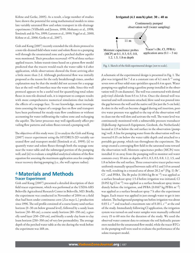
Application of Eq. [1–4] to the fi eld tracer experiment using HYDRUS-2D requires defi nition of the numeri-cal finite element mesh, the initial and boundary conditions, and the soil hydraulic and solute trans-port parameters. We considered an axisymmetrical fl ow fi eld of 250-cm height and a radius of 3000 cm (Fig. 2). Vertical extension of the simulation domain was chosen due to the existence of a nearly imperme-able clay layer at the depth of 250 cm that prevented deep leaching and caused lateral water movement and solute transport. Th e grid origin (radius r = 0, depth z = 0) was set at the center of the observation well and at a depth of 250 cm from ground level. Th e fi nite ele-ment mesh size was 5 cm in the vertical direction and

10 cm in the horizontal direction everywhere, except near the soil surface and the well boundary, where we used a mesh size of 2.5 cm. Th e low-permeability clayey bed at the bottom of the simula-tion domain was considered to be a no-fl ux boundary for both fl ow and solute transport. Along the right boundary, 30 m from the pumping well, we assumed that the water table depth (1.68 m) was not aff ected by the irrigation by imposing an equilibrium pres-sure head distribution vs. depth for fl ow and a zero concentration gradient for transport.

Th e soil surface boundary was divided into four concentric rings (Fig. 2). A constant water fl ux of 4.1 mm h−1 was imposed between radii of 2.5 to 2000 cm and a zero fl ux elsewhere. A solute fl ux with concentration equal to the concentration of the irrigation water (Cir) was assigned between radii of 2.5 and 10 cm and between 300 and 2000 cm. Water and solute fl uxes were assumed to be zero for radii >2000 cm. Flux concentrations between 10 and 300 cm near the well where the tracers were applied were calculated such that they were consistent with the total tracer application rates. We assumed pulse durations of 1 h (related to the dissolution times) for all tracers, leading to concentrations of the infi ltrating water of 25.95, 12.69, and 4.07 g L−1 for Br, Cl, and PFBA, respectively. Th e Cl concentration of the irrigation water was 8.75 mg L−1 (Gish and Kung, 2007), while no Br or PFBA were present in the irriga-tion water.

Along the left boundary (at r = 2.5 cm) representing the well, a seepage face was allowed to develop above the water level in the well. Although the model stipulated a potential seepage boundary from the elevation of 85 cm to the soil surface, the “active” seep-age face occurs only near the water table (see Fig. 2), depending on the transient fl ow conditions during the experiment. During simulation, the saturated part (ψ ≥ 0) of a potential seepage face is treated as a prescribed pressure head boundary with ψ = 0, while the unsaturated part (ψ < 0) is treated as a prescribed zero fl ux (Fig. 2). Th e lengths of the two surface segments are continually adjusted (Neuman, 1975) during the iterative process until the

Fig. 2. Simulation domain with the invoked boundary conditions (not to scale). Th e profi le consisted of fi ve diff erent layers (Layer 2 is divided into two sublayers; Layer 5 is composed of low-permeability clay loam and is not included in the simulation domain); CT and Cir are solute concentrations of the infi ltrating water.

www.VadoseZoneJournal.org | 689

calculated values of fl ux along the saturated part, and the calcu-lated values of ψ along the unsaturated part, are all negative, thus indicating that water is leaving the fl ow region through the satu-rated part of the surface boundary only.

Additionally, a variable fl ux (Neumann boundary condition) was specifi ed between the elevations of 5 and 80 cm in the submerged well zone (Fig. 2) where the pump was installed. A more rigorous procedure would be to specify equilibrium pressure head distri-bution (Gardner, 2005; Wilson and Gardner, 2006) based on transient water levels measured by the pressure transducer; how-ever, the obtained data exhibited a highly oscillating water level due to non-uniform pumping rates and relatively small water vol-umes in the well, which makes it diffi cult to prescribe transient pressure head values. Another reason why we used the variable fl ux boundary instead of a prescribed pressure head is that we wanted to preserve water fl uxes pumped from the well. Note that we did not need to account for any loss in fl ows due to plugged well slots. Th e imposed variable fl ux through the submerged well boundary was adjusted iteratively during the numerical calculations. We started by prescribing the fl ux values equal to the pumping rate, and calcu-lated the total water volume out of the well boundary (a sum of the seepage fl ow and the variable fl ux), which signifi cantly exceeded the total volume pumped. We gradually decreased the imposed values of variable fl ux until the simulated total fl ow volume along the well boundary matched the measured total volume of pumped water at the end of the simulation period. Finally, a zero concentra-tion gradient was assumed along the left and right boundaries of the transport domain.

As the initial condition for the pressure head we used an equi-librium distribution in the profi le corresponding to the observed initial water table elevation of 82 cm. Th e initial concentrations for the transport simulations were zero for Br and PFBA and 7.3 mg L−1 for Cl, being the average measured Cl concentration in the saturated zone before irrigation.

Calculated Tracer Concentra ons in the Pumping WellSolute concentrations of the pumped water (Cw) were calculated from a mass balance equation assuming full mixing in the pump-ing well as follows:

( ) ( ) ( )π = + −2 ww w c(SF) c(VB) p w

ddC

r h Q t Q t Q t Ct

[5]

where rw is the well radius [L], hw is the time-averaged mean water level in the well measured from the well base [L], Qc(SF) and Qc(VB) are the mass fl uxes [M T−1] of the tracers to the well through the seepage face and variable fl ux boundaries, respectively, as calcu-lated with HYDRUS-2D, and Q p is the pumping rate [L3 T−1]. We used the time-averaged mean water level in the well because the actual record exhibited highly oscillating values. In fact,

simulations indicated that the eff ect of hw on concentration was not signifi cant due to the relatively small water volume in the well and the large water and solute fl uxes.

Th e goodness-of-fi t of the model was evaluated using the coeffi cient of determination (R2) and the modifi ed index of agreement (MIA) as given by Legates and McCabe (1999):

( ) ( )

( ) ( )=

= =

=

−−

− + −

∑∑ ∑

obsw w1

obs obs obsw w w w1 1

MIA

1n

i iin n

i ii i

C t C t

C t C C t C

[6]

where Cw(ti) and Cwobs(ti) represent the simulated and observed

concentrations of a tracer in pumped water at time ti, and obswC is

the mean observed concentration. While there is no statistical basis to decide exactly which MIA value is a good threshold character-izing the use of an “accurate” model, following Köhne et al. (2005) we assumed simulations with MIA > 0.75 as being “accurate.”

Inverse Solu on for the Unsaturated Soil Hydraulic ParametersTh e soil hydraulic parameters needed for the calculations were esti-mated using a combination of one- and two-dimensional inverse simulations performed with the HYDRUS-1D (Šimůnek et al., 2005) and HYDRUS-2D soft ware packages, respectively, as well as laboratory measurements of the saturated water content (θs) of the various soil horizons. During a fi rst step, we used HYDRUS-1D to estimate the hydraulic parameters from the observed water content values that were monitored at diff erent depths in the soil profi le 11 m away from the pumping well. By using HYDRUS-1D we assumed that fl ow in the unsaturated zone relatively far (11 m) from the pumping observation was mainly in the vertical direc-tion, thus considerably minimizing computational times compared with using HYDRUS-2D. During the second step, we used HYDRUS-2D to perform additional calibrations of the saturated hydraulic conductivity (Ks) of Layers 3 to 5 (Fig. 2), where water presumably fl owed both vertically and horizontally.

For the HYDRUS-1D simulations, we assumed a 250-cm-deep soil profi le consisting of fi ve layers consistent with the described lithology of the site: loamy sand at 0–30 cm, sandy loam at 30–50 cm, sandy loam at 50–80 cm, coarse sand at 80–140 m, and gravely sand at 140–250 m. Th e clay loam horizon (250–350 cm) had an extremely low conductivity and as such was considered imperme-able and hence not included in the simulations. Th e sandy loam horizon (30–80 cm) was subdivided into two layers based on the fact that markedly diff erent water contents were observed during steady infi ltration at depths of 30 and 50 cm, thus indicating dif-ferent hydraulic properties. Th e MCP-measured water content at depths of 10, 30, 50, 80, 120, and 150 cm were used to calibrate the fl ow model, which in total contained 25 hydraulic parameters (the fi ve parameters θr, θs, α , n, and Ks for each of the fi ve layers). To

www.VadoseZoneJournal.org | 690

minimize issues of uniqueness in the inverse solution, we decreased the number of optimized parameters by using experimentally measured values of the water content at saturation (θs), and zero values of the residual water content (θr) for all coarse-textured layers (except sandy loam). Th us, we needed to determine three parameters (Ks, α, and n) for each of the fi ve layers and one θr value for the sandy loam horizon.

Th e experiment was conducted in November of 2004 when air temperatures ranged from 1 to 7°C, the evaporation rate was low, and no rain or irrigation occurred in the week before the experiment (Gish and Kung, 2007). Th erefore, we assumed that the initial pressure head profi le was close to equilibrium with the water table at 168 cm. Th e boundary condition at the soil surface defi ned a water fl ux of 4.1 mm h−1 during the irrigation period. Since the bottom boundary at 250 cm was considered to be imper-meable, the water table was likely to rise at some distance around the well aft er irrigation began. As a result, some lateral water fl ow in the saturated zone occurred, which had to be accounted for by the fl ux through the lower boundary in the one-dimensional HYDRUS-1D simulations. Th is fl ux varied with time, depending on the position of the water table. To simulate this process, we used the HYDRUS-1D horizontal drain boundary condition with a drain spacing of 22 m (twice the distance from the MCP location to the pumping well). Although this boundary condition does not describe the physical two-dimensional fl ow system exactly, it was the boundary condition available in HYDRUS-1D that most closely represented our fi eld conditions.

Initial estimates of the α and n parameters for the inverse proce-dure were based on the assumed initial equilibrium distribution of the pressure head and the observed water contents before the experiment, while Ks values were initially estimated from soil textural class and particle size distribution information. We used a sequential inverse procedure by starting the parameter search with the fi rst layer, while assuming that the other parameters were known (the initial estimates) and using observed water contents of the 10-cm depth only. Th e next step was to fi nd parameters of the second layer by fi tting water contents at depths of 0.1 and 0.3 m, and using the parameters of the fi rst layer found at the previ-ous step. Th e third step was to adjust the parameters of Layers 1 and 2 simultaneously by fi tting the measured water contents at depths of 0.1 and 0.3 m. We continued this sequential procedure by gradually increasing the number of layers and hence the number of parameters that were simultaneously estimated. During the fi nal step, the code searched simultaneously for 15 parameters (θr for the sandy loam horizon was not changed aft er the third run).

Well Capture Zone under Steady-State Condi onsTh e recovery of the tracers is an important factor that allows assess-ment of the solute mass balance. In a radially convergent, saturated fl ow fi eld, the recovery depends on the tracer application radius

and the well capture zone. To avoid losses of the tracer with lateral fl ow, the radius must be less than the radius of the water table divide, where the radial fl ow velocity is equal to zero (Fig. 3). Th e radius of the water table divide can be roughly estimated from a solution of the Boussinesq equation for steady-state radial uncon-fi ned fl ow toward a well, subject to Dirichlet boundary conditions as follows:

( )⎛ ⎞∂ ∂ ⎟⎜ =− − ≤ ≤⎟⎜ ⎟⎜⎝ ⎠∂ ∂s 0

1 hK rh iH a r r a R

r r r [7]

= =0 0:r r h h [8]

= =: Rr R h h [9]

where h is the water table height [L], Ks is the hydraulic conductiv-ity of the aquifer, i is the recharge rate [L T−1], H(r) is the Heaviside step function, a is the radius of the infi ltration area (r0 ≤ a ≤ R), r0 and R are the radii of the well and the outer boundary [L], respectively, h0 and hR are the water table heights at r = r0 and r = R, respectively, and r is the radial coordinate.

Assuming a constant hydraulic conductivity, Ks, and integrating Eq. [7], we obtained an analytical expression for the radial water fl ux to the well, Q:

( ) ( )

( )

( )

∂=− π

∂⎧ ⎫⎪ ⎪− − −⎪ ⎪⎪ ⎪⎪ ⎪⎛ ⎞⎪ ⎪− ⎟⎪ ⎪⎜⎪ ⎪⎟⎜− + += π⎨ ⎬⎟⎜ ⎟⎟⎪ ⎪⎜⎝ ⎠⎪ ⎪⎪ ⎪−⎪ ⎪⎪ ⎪⎪ ⎪⎪ ⎪⎩ ⎭

2 2

2 22 2 20

0

0

2

ln2

ln

R

hQ Krh

rir H a r ia H r a

a r Rh h K i aa

R r

[10]

Fig. 3. Schematic of unconfi ned radial fl ow with infi ltration; r, radial coordinate; a, radius of infi ltration area; r*, well capture radius; h, water table height; r0 and R, radii of well and outer boundary, respec-tively; h0 and hR, water table heights at r = r0 and r = R, respectively; Q, radial water fl ux.

www.VadoseZoneJournal.org | 691

For the limiting case of a = R, this solution coincides with an equation derived by Aravin and Numerov (1965).

An equation for the water table divide radius (r*) may be obtained by solving the equation for Q = 0 for the case when r* < a:

( )( )

⎛ ⎞− ⎟⎜ ⎟⎜− + + ⎟⎜ ⎟⎟⎜⎝ ⎠=

2 22 2 2s 0

0

0

ln2

*ln

RK a r Rh h ai a

rR r

[11]

Th e pumping well discharge is calculated from

( )( )

=∂

=− π∂

⎧ ⎫⎛ ⎞⎪ ⎪− ⎟⎪ ⎪⎜ ⎟⎪ ⎜ ⎪− + + ⎟⎜⎪ ⎪⎟⎟⎜⎪ ⎪⎝ ⎠⎪ ⎪= π −⎨ ⎬⎪ ⎪⎪ ⎪⎪ ⎪⎪ ⎪⎪ ⎪⎪ ⎪⎩ ⎭

0 00 s 0

2 22 2 20

0 s20

0

2

ln2

ln

r r r

R

hQ r K h

ra r Rh h K i a

air

R r

[12]

Results and DiscussionUnsaturated Soil Hydraulic ParametersFigure 4 compares the MCP-measured water contents at diff erent depths with the simulated values obtained with HYDRUS-1D. Good agreement was obtained between the observed and simu-lated water contents for all depths except at 0.8 m, for which R2 = 0.877. Th e fl uctuations in observed water contents at the four upper observation points may have been caused by non-uniform irrigation during several windy days (Gish and Kung, 2007). Th e calculated water content time series clearly describes the propaga-tion of the moisture front into the profi le.

Table 1 presents the fi tted hydraulic parameters obtained using the invoked inverse procedure. Th e values of α and n are within the range reported by Hodnett and Tomasella (2002) for soils with similar textures. A relatively high value of 10 was obtained for the van Genuchten hydraulic parameter n for the fi ft h layer (gravely sand), which implies a very steep water retention curve and an unsaturated hydraulic conductivity curve in which the conduc-tivity decreases very rapidly with decreasing pressure head. While some slight changes in the minimized objective function occurred when the parameter n varied between 8 and 12, the simulated water contents were found not to be sensitive to these changes. We therefore accepted a value of n = 10 for the very coarse-textured gravelly sand layer. Th e saturated hydraulic conductivity for the loamy sand and sandy loam (Layers 1 and 2, Table 1) seemingly has extremely high values, yet these values were obtained as a result of inverse simulations for the limited range of water content in the unsaturated zone and for the most common value of the pore-connectivity parameter τ = 0.5 (Eq. [4]). Th e value of τ can vary in a range from −1 to 2.5 (Mualem, 1976), however, and Schuh

and Cline (1990) reported that τ varied between −8.73 and 14.80. Th is most signifi cantly aff ects the hydraulic conductivity values at water content close to saturation. Th us, the obtained Ks values for Layers 1 and 2 have a great deal of uncertainty and should not be used to simulate saturated conditions.

Additional calibrations were performed with the complete two-dimensional axisymmetrical fl ow model against the observed water contents. As a result, we obtained values for Ks of 185, 149, and 52 cm h−1 for Layers 2-2 (sandy loam), 3 (coarse sand), and 4 (gravely sand), respectively. Th e maximum diff erence of these Ks values from those obtained for the one-dimensional problem was for the fourth layer. Th e calibrated Ks for the two-dimensional problem here was approximately one-third than that of the one-dimensional problem (Table 1). Th is diff erence was probably due to using an imperfect lower boundary condition in the one-dimensional case. Th e simulated water contents obtained with HYDRUS-2D were essentially identical to those shown in Fig. 4. For the two-dimen-sional calibration R2 = 0.858, slightly smaller than the value of 0.877 obtained with the HYDRUS-1D calibration.

Fig. 4. Observed (circles) and simulated (lines) water contents at diff erent depths.

Table 1. Unsaturated soil hydraulic parameters† inversely estimated using HYDRUS-1D.

Layer Depth θs‡ θr α n Ks

cm cm−1 cm h−1

1 0–30 0.327 0 0.046 1.62 100

2-1 30–50 0.351 0.024 0.054 1.46 115

2-2 50–80 0.260 0 0.054 1.33 113

3 80–150 0.315 0 0.069 1.76 161

4 150–250 0.330 0 0.044 10.00 167

† θs and θr, saturated and residual water contents, respectively; α and n, shape parameters; Ks, saturated hydraulic conductivity.

‡ Experimentally determined.

www.VadoseZoneJournal.org | 692

Despite the achieved good fi t to the experimental data, we realize that the obtained set of parameters may not be unique and that additional experiments would be helpful to reduce uncertainty in the parameters. Nevertheless, we accepted these values and then used them for our simulations for the two-dimensional case. Of course, the objective of our study was to obtain an accurate description of the experimental fi eld data (water contents, fl ow rates, and concentrations of the well water), rather than unique soil hydraulic parameters. Th is is reasonable since no attempts were made to extrapolate the data observed beyond the experimental time period.

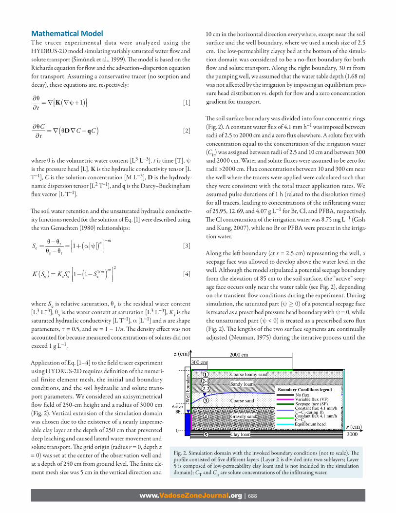
Two-Dimensional Simula ons of Water Flow and Solute TransportSolute transport simulations were performed for four different values of the longitudinal dispersivity, aL (5, 15, 25, and 40 cm). Th ese values are within the range of 0.05 to 1 m obtained from the fi eld tracer tests (Gelhar et al., 1992). We used the same value for all layers, while assuming in most cases a ratio of 10 between the longitudinal (aL) and transversal (aT) dispersivities. Th is ratio is well within the range of ratios (5–20) reported in several studies by Anderson (1979) and Domenico and Schwartz (1998, p. 506). For unsaturated soils, the variability in fl ow direction and microscopic velocity can be larger than in saturated soils because of the lower degree of water saturation (Maraqa et al., 1997; Nützmann et al., 2002). A clear relationship between the degree of saturation and the dispersivity has not yet been established, however, and therefore we used constant values of these parameters for the entire variably satu-rated domain. Figure 5 compares the observed and calculated (using Eq. [5]) solute BTCs of the tracers in the well. Th e results are shown for simulations with and without accounting for the seepage face. Neglecting the seepage face boundary caused a delay of a few hours in the arrival of the solute fronts as well as of the maximum con-centration, except those of PFBA. Th e PFBA was applied 7 h aft er the experiment began and the fl ow conditions in the unsaturated zone were diff erent than at the beginning. Th e peak concentrations decreased somewhat, except perhaps for Cl (Fig. 5b). Because overall agreement with the experimental data was better when the seepage face was considered, we will focus primarily on results obtained for simulations with the seepage face boundary.

Th e best agreement between the observed and simulated BTCs of the tracers in the well was obtained when we used a value of 15 cm for aL (Fig. 5). Th e R2 values were 0.909, 0.899, and 0.930 and the MIA criterion (Eq. [6]) was 0.883, 0.857 and 0.896 for Br, Cl, and PFBA, respectively. Th e model provided a good descrip-tion of the tracer arrival in the well, but overestimated the arrival time of the maximum concentration by around 8.7%. Simulations with a dispersivity of 5 cm improved the description of the front part of the solute BTCs (especially the initial slope) but caused much lower tails. On the other hand, simulations with a disper-sivity of 40 cm described the tails quite well but resulted in much earlier arrival times and lower maximum concentrations than the

observed values. Decreasing the ratio aL/aT from 10 to 5 did not have an appreciable impact on the simulated BTCs.

Th e steeper arrival fronts, more pronounced asymmetrical shape, earlier concentration peaks, and longer tails of the observed BTCs compared with the simulated curves (Fig. 5) may indicate enhanced preferential fl ow or an underestimation of the soil heterogeneity in the simulations (Kung et al., 2000; Buczko and Gerke, 2006).

Fig. 5. Observed (circles) and simulated solute breakthrough curves of (a) Br, (b) Cl, and (c) pentafl uorobenzoic acid (PFBA). Simulations were obtained with (solid lines) and without (dashed lines) account-ing for a seepage face boundary.

www.VadoseZoneJournal.org | 693

Some of these features probably could be accounted for by invok-ing a scale-dependent dispersivity in the model; however, limited soil data were available. Th e variability in the observed concentra-tions at about the time when the peak concentrations were detected (Fig. 5) may have been caused by an unsteady pumping rate (the pumping rate generally increased with time) and because the pump had to be replaced at some point during the experiment (Gish and Kung, 2007). Th e simulated BTCs (Fig. 5) also exhibited oscil-lating behavior during the time interval when the pumping rate fl uctuated signifi cantly. Th e latter caused changes in the seepage face length and in the values of solute fl uxes through the seepage face and the submerged part of the well. Abrupt changes in these fl uxes and in their ratio induced the oscillation of simulated con-centrations in the well.

Th e sensitivity of the model to the assumed dissolution times of the tracers at the soil surface was also evaluated. A fourfold decrease or increase in the pulse duration (0.25 or 4 h, respectively) and conse-quently a four times increase or decrease in the surface boundary concentration (to preserve the injected tracer masses) were found to produce similar results. We additionally tested the eff ect of having a diff erent thickness of the fi ft h layer (where most of the well screen was located) by moving the lower boundary of the fl ow domain up to 2.3 m or down to 2.7 m below the soil surface (Fig. 2). Simulation results showed that this did not aff ect the arrival time of the tracers. Th e front and back (receding) parts of the BTCs were slightly steeper, while the maximum concentration in the well was about 10% larger for the thicker fi ft h layer (bottom boundary at 2.7 m) than with a 2.3-m-deep bottom boundary.

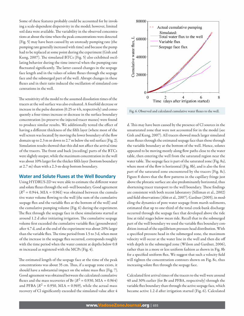
Water and Solute Fluxes at the Well BoundaryUsing HYDRUS-2D we were able to estimate the diff erent water and solute fl uxes through the soil–well boundary. Good agreement (R2 = 0.944, MIA = 0.961) was obtained between the cumula-tive water volume fl owing to the well (the sum of the cumulative seepage fl ux and the variable fl ux at the bottom of the well) and the cumulative pumping volume (Fig. 6) during the experiment. Th e fl ux through the seepage face in these simulations started at around 1.2 d aft er initiating irrigation. Th e cumulative seepage volume fi rst exceeded the cumulative variable fl ux (groundwater) aft er 4.7 d, and at the end of the experiment was about 20% larger than the variable fl ux. Th e time period from 1.5 to 3 d, when most of the increase in the seepage fl ux occurred, corresponds roughly with the time period when the water content at depths below 0.8 m increased as registered with the MCPs (Fig. 4).

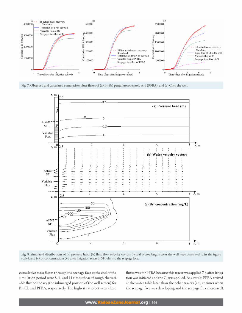
Th e estimated length of the seepage face at the time of the peak concentrations was about 35 cm. Th us, if a seepage zone exists, it should have a substantial impact on the solute mass fl ux (Fig. 7). Good agreement was obtained between the calculated cumulative fl uxes and the mass recoveries of Br (R2 = 0.930, MIA = 0.964) and PFBA (R2 = 0.950, MIA = 0.969), while the actual mass recovery of Cl signifi cantly exceeded the simulated value aft er 4

d. Th is may have been caused by the presence of Cl sources in the unsaturated zone that were not accounted for in the model (see Gish and Kung, 2007). All tracers showed much larger simulated mass fl uxes through the estimated seepage face than those through the variable boundary at the bottom of the well. Hence, solutes appeared to be moving mostly along fl ow paths close to the water table, then entering the well from the saturated region near the water table. Th e seepage face is part of the saturated zone (Fig. 8a), where most of the fl ow is horizontal (Fig. 8b), and is also the fi rst part of the saturated zone encountered by the tracers (Fig. 8c). Figure 8 shows that the fl ow patterns in the capillary fringe just above the phreatic surface are also predominantly horizontal, thus shortening tracer transport to the well boundary. Th ese fi ndings are consistent with both recent laboratory (Silliman et al., 2002) and fi eld observations (Abit et al., 2007). Gardner (2005), in mod-eling the dynamics of pore water seepage from marsh sediments, estimated that up to one-third of the total creek-bank discharge occurred through the seepage face that developed above the tide line at tidal stages below mean tide. Recall that in the submerged part of the well boundary we used the variable fl ux boundary con-dition instead of the equilibrium pressure head distribution. With a specifi ed pressure head in the submerged zone, the maximum velocity will occur at the water line in the well and then die off with depth in the submerged zone (Wilson and Gardner, 2006), rather than in a more or less uniform fashion as shown in Fig. 8b for a specifi ed uniform fl ux. We suggest that such a velocity fi eld will tighten the concentration contours shown on Fig. 8c, thus increasing solute fl ux through the seepage face.

Calculated fi rst arrival times of the tracers to the well were around 40 and 30% earlier (for Br and PFBA, respectively) through the variable fl ux boundary than through the active seepage face, which became active 1.2 d aft er irrigation started (Fig. 6). Calculated

Fig. 6. Observed and calculated cumulative water fl uxes to the well.

www.VadoseZoneJournal.org | 694

cumulative mass fl uxes through the seepage face at the end of the simulation period were 8, 4, and 11 times those through the vari-able fl ux boundary (the submerged portion of the well screen) for Br, Cl, and PFBA, respectively. Th e highest ratio between these

fl uxes was for PFBA because this tracer was applied 7 h aft er irriga-tion was initiated and the Cl was applied. As a result, PFBA arrived at the water table later than the other tracers (i.e., at times when the seepage face was developing and the seepage fl ux increased).

Fig. 8. Simulated distributions of (a) pressure head, (b) fl uid fl ow velocity vectors (actual vector lengths near the well were decreased to fi t the fi gure scale), and (c) Br concentrations 3 d aft er irrigation started; SF refers to the seepage face.

Fig. 7. Observed and calculated cumulative solute fl uxes of (a) Br, (b) pentafl uorobenzoic acid (PFBA), and (c) Cl to the well.

www.VadoseZoneJournal.org | 695

Th e smallest ratio between the seepage solute fl ux and the variable fl ux was for Cl due to its immediate input from the saturated zone having a background concentration of 7.3 mg L−1. Our results are very much in agreement with sand box experimental and model-ing results by Li et al. (2007), who studied the impact of a seepage face at an unconfi ned aquifer–lake interface. Th ey found that most of the groundwater fl ow and pollutant fl ux discharged through a narrow portion near the top of the seepage face.

Well Capture ZoneTo avoid solute losses with lateral fl ow away from the well, the radius of a tracer surface application should be smaller than the radius of the well capture zone. Th e results of simulations with the HYDRUS-2D code indicate that the water table divide was located at about 620 cm from the well. An approximate estimate of the well capture radius can also be obtained with Eq. [11], which assumes steady-state fl ow conditions. Such conditions probably occurred during Days 3 to 5 of the experiment when the pump-ing rate varied very little around a mean value of 0.12 L s−1. Th e assumption of steady-state fl ow was further confi rmed by the HYDRUS-2D simulations. Using Eq. [11] and [12], we estimated the well capture radius (r*) of our fi eld tracer experiment to be 580 cm and the pumping discharge rate (Qr0) to be 0.12 L s−1. For the calculations, we used r0 = 2.5 cm, R = 3000 cm, a = 2000 cm, K = 52 cm h−1, i = 0.41 cm h−1, h0 = 90 cm, and hR = 82 cm. Th e values of both r* and Qr0 decreased with increasing hydraulic conductivity (Fig. 9).

Th e analytical solutions for r* (Eq. [11]) and Qr0 (Eq. [12]) were obtained with several simplifying assumptions such as steady fl ow, having a homogeneous aquifer, and no seepage face. Th is caused Eq. [12] to underestimate the well capture radius com-pared with the more comprehensive HYDRUS-2D hydrodynamic model. Nevertheless, this example demonstrates that for practical purposes the analytical solution can provide a useful fi rst approxi-mation of system parameters needed for the design of these types of tracer experiments.

ConclusionsTh e HYDRUS-2D simulations of the fi eld tracer experiment (Gish and Kung, 2007), in which three surface-applied tracers moved through the unsaturated zone to a pumping well in a perched shal-low aquifer, indicate the presence of a seepage face boundary in the well near the water table. Transport simulations were performed for several scenarios with diff erent aL values. Values of aL varied from 5 to 40 cm, while keeping the aL/aT ratio at 10. Th e best over-all results were obtained with a longitudinal dispersivity of 15 cm. Th e observed tracer breakthrough curves exhibited steeper rising fronts, more pronounced asymmetry, earlier concentration peaks, and longer tails than the simulated curves without a seepage face. Including a seepage face improved the predictions by causing earlier breakthrough times and higher solute concentrations in the well.

Good agreement was obtained between the observed and simu-lated cumulative water and solute fl uxes to the well. Th e simulation results indicated that the cumulative water fl ux to the well through the seepage face at the end of the experiment was about 20% larger than the cumulative variable fl ux through the saturated zone. Th e calculated cumulative seepage face fl uxes of the tracers were approximately 8, 4, and 11 times the variable fl ux boundary for Br, Cl, and PFBA, respectively. Th ese signifi cant diff erences can be partially explained by the presence of higher solute concentra-tions in the capillary fringe and in the upper part of the saturated zone compared with the lower saturated zone (connected to the submerged portion of the well). Th e higher concentrations from the soil solution discharged to the well through the seepage face of the unconfi ned aquifer. Our study further suggests that a seepage face should be considered when evaluating solute fl uxes using this mass fl ux well transport approach.

It must also be realized that an alternative conceptual model, e.g., simulating preferential fl ow through a high-hydraulic-conductivity layer below the water table, can provide a similar or an even better fi t to the observed BTC. Using the preferential fl ow and deterministic transport model, however, requires knowledge of additional param-eters that cannot be assessed with the existing data set. We believe that such a model would also predict the development of the seepage face; however, the ratio between the solute fl uxes through the seep-age face and through submerged part of the well would be diff erent from that obtained with the conventional model.

AcknowledgmentsTh is work has been partially supported through the Interagency USDA and U.S. NRC Agreement RES-02-008 “Model Abstraction Techniques for Soil Water Flow and Transport.”

Fig. 9. Well capture radius (r*) and pumping rate (Qr0) as a function of hydraulic conductivity (Ks) for a given set of parameters (radius of the well [r0], 2.5 cm; radius of the outer boundary [R], 3000 cm; radius of the infi ltration area, 2000 cm; recharge rate, 0.41 cm h−1; water table height at radial coordinate r = r0, 90 cm; water table height at r = R, 82 cm).

www.VadoseZoneJournal.org | 696

ReferencesAbit, S.M., A. Amoozegar, M.J. Vepraskas, and C.P. Niewoehner. 2007. Solute

transport in the capillary fringe and shallow groundwater: Field evalua- on. Vadose Zone J. 7:890–898.

Anderson, M.P. 1979. Using models to simulate the movement of contami-nants through groundwater fl ow systems. Crit. Rev. Environ. Control 9:97–156.

Aravin, V.I., and S.N. Numerov. 1965. Theory of fl uid fl ow in undeformable porous media. Israel Prog. for Sci. Transl., Jerusalem.

Bear, J. 1972. Dynamic of fl uids in porous media. Elsevier, New York.Buczko, U., and H.H. Gerke. 2006. Modeling two-dimensional water fl ow and

bromide transport in a heterogeneous ligni c mine soil. Vadose Zone J. 5:14–26.

Chenaf, D., and R.P. Chapuis. 2007. Seepage face height, water table posi on, and well effi ciency at steady state. Ground Water 45:168–177.

Domenico, P.A., and F.W. Schwartz. 1998. Physical and chemical hydrogeol-ogy. 2nd ed. John Wiley & Sons, New York.

Gardner, L.R. 2005. The role of geomorphic and hydraulic parameters in governing pore water seepage from salt marsh sediments. Water Resour. Res. 41:W07010, doi:10.1029/2004WR003671.

Gelhar, L.W., A. Mantaglou, C. Welty, and K.R. Rehfeldt. 1992. A cri cal review of fi eld-scale dispersion in aquifers. Water Resour. Res. 28:1955–1974.

Gerke, H.H., J. Dusek, T. Vogel, and J.M. Köhne. 2007. Two-dimensional dual-permeability analyses of a bromide tracer experiment on a le-drained fi eld. Vadose Zone J. 6:651–667.

Gish, T.J., and K.-J.S. Kung. 2007. Procedure for quan fying a solute fl ux to a shallow perched water table. Geoderma 138:57–64.

Gish, T.J., K.-J.S. Kung, D.C. Perry, J. Posner, G. Bubenzer, C.S. Helling, E.J. Klad-ivko, and T.S. Steenhuis. 2004. Impact of preferen al fl ow at varying ir-riga on rates by quan fying mass fl uxes. J. Environ. Qual. 33:1033–1040.

Hodne , M.G., and J. Tomasella. 2002. Marked diff erences between van Genuchten soil water-reten on parameters for temperate and tropical soils: A new water-reten on pedo-transfer func ons developed for tropi-cal soils. Geoderma 108:155–180.

Kladivko, E.J., L.C. Brown, and J.L. Baker. 2001. Pes cide transport to subsur-face le drains in humid regions of North America. Crit. Rev. Environ. Sci. Technol. 31:1–61.

Köhne, J.M., and H.H. Gerke. 2005. Spa al and temporal dynamics of pref-eren al tracer movement towards a le drain. Vadose Zone J. 4:79–88.

Köhne, J.M., B.P. Mohanty, and J. Šimůnek. 2005. Inverse dual-permeability modeling of preferen al water fl ow in a soil column and implica ons for fi eld-scale solute transport. Vadose Zone J. 5:59–76.

Köhne, S., B. Lennartz, J.M. Köhne, and J. Šimůnek. 2006. Bromide trans-port at a le-drained fi eld site: Experiment, and one- and two-dimen-sional equilibrium and non-equilibrium numerical modeling. J. Hydrol. 321:390–408.

Kung, K.-J.S., E.J. Kladivko, T.J. Gish, T.S. Steenhuis, G. Bubenzer, and C.S. Helling. 2000. Quan fying preferen al fl ow by breakthrough of sequen- ally applied tracers: Silt loam soil. Soil Sci. Soc. Am. J. 64:1296–1304.

Larsson, M.H., N.J. Jarvis, G. Torstensson, and R. Kasteel. 1999. Quan fy-ing the impact of preferen al fl ow on solute transport to le drains in a sandy fi eld soil. J. Hydrol. 215:116–134.

Legates, D.R., and G.J. McCabe, Jr. 1999. Evalua ng the use of “goodness-of-fi t” measures in hydrologic and hydroclima c model valida on. Water Resour. Res. 35:233–241.

Li, Y., C. Wang, L.-Z. Yang, and Y.-P. Li. 2007. Infl uence of seepage face obliq-uity on discharge of groundwater and its pollutant into lake from a typi-cal unconfi ned aquifer. J. Hydrodyn. Ser. B. 19:756–761.

Maraqa, M.A., R.B. Wallace, and T.C. Voice. 1997. Eff ects of degree of water satura on on dispersivity and immobile water in sandy soil columns. J. Contam. Hydrol. 25:199–218.

Mohanty, B.P., J.M. Bowman, J.M.H. Hendrickx, J. Šimůnek and M.Th. van Genuchten. 1998. Preferen al transport of nitrate to a le drain in an intermi ent-fl ood-irrigated fi eld: Model development and experimental evalua on. Water Resour. Res. 34:1061–1076.

Mualem, Y. 1976. A new model predic ng the hydraulic conduc vity of un-saturated porous media. Water Resour. Res. 12:513–522.

Neuman, S.P. 1975. Galerkin approach to saturated–unsaturated fl ow in po-rous media. p. 201–217. In R.H. Gallagher et al. (ed.) Finite elements in fl uids. Vol. 1. Viscous fl ow and hydrodynamics. John Wiley & Sons, London.

Nützmann, G., S. Maciejewski, and K. Joswig. 2002. Es ma on of water satu-ra on dependence of dispersion in unsaturated porous media: Experi-ments and modelling analysis. Adv. Water Resour. 25:565–576.

Petersen, C.T., J. Holm, C.B. Koch, H.E. Jensen, and S. Hansen. 2002. Move-ment of pendimethalin, ioxinyl and soil par cles to fi eld drainage les. Pest Manag. Sci. 59:85–96.

Rushton, K.R. 2006. Signifi cance of a seepage face on fl ows to wells in uncon-fi ned aquifers. Q. J. Eng. Geol. Hydrogeol. 39:323–331.

Schuh, W.M., and R.L. Cline. 1990. Eff ect of soil proper es on unsaturated hydraulic conduc vity pore-interac on factors. Soil Sci. Soc. Am. J. 54:1509–1519.

Shamsai, A., and T.N. Narasimhan. 1991. A numerical inves ga on of free surface–seepage face rela onship under steady state fl ow condi ons. Water Resour. Res. 27:409–421.

Silliman, S.E., B. Berkowitz, J. Šimůnek, and M.Th. van Genuchten. 2002. Fluid fl ow and solute migra on within the capillary fringe. Ground Water 40:76–84.

Simpson, M.J., T.P. Clement, and T.A. Gallop. 2003. Laboratory and numeri-cal inves ga on of fl ow and transport near a seepage-face boundary. Ground Water 41:690–700.

Šimůnek, J., and J.A. de Vos. 1999. Inverse op miza on, calibra on and vali-da on of simula on models at the fi eld scale. p. 431–445. In J. Feyen and K. Wiyo (ed.) Modelling transport processes in soils at various scales in me and space. Wageningen Pers, Wageningen, the Netherlands.

Šimůnek, J., M. Sejna, and M.Th. van Genuchten. 1999. The HYDRUS-2D so ware package for simula ng the two-dimensional movement of wa-ter, heat, and mul ple solutes in variably-saturated media. Version 2.0. IGWMC-TPS-53. Int. Ground Water Modeling Ctr., Colorado School of Mines, Golden.

Šimůnek, J., M.Th. van Genuchten, and M. Sejna. 2005. The HYDRUS-1D so -ware package for simula ng the one-dimensional movement of water, heat, and mul ple solutes in variably-saturated media. Version 3.0. Dep. of Environ. Sci., Univ. of California, Riverside.

Vachaud, G., and M. Vauclin. 1975. Comments on “A numerical model based on coupled one-dimensional Richards and Boussinesq equa ons.” Water Resour. Res. 11:506–509.

van Genuchten, M.Th. 1980. A closed-form equa on for predic ng the hy-draulic conduc vity of unsaturated soils. Soil Sci. Soc. Am. J. 44:892–898.

Villholth, K.G., and K.H. Jensen. 1998. Flow and transport processes in a mac-roporous subsurface-drained glacial ll soil: II. Model analysis. J. Hydrol. 207:121–135.

Vogel, T., H.H. Gerke, R. Zhang, and M.Th. van Genuchten. 2000. Modeling fl ow and transport in a two-dimensional dual-permeability system with spa ally variable hydraulic proper es. J. Hydrol. 238:78–89.

Wilson, A.M., and L.R. Gardner. 2006. Tidally driven groundwater fl ow and solute exchange in a marsh: Numerical simula ons. Water Resour. Res. 42:W01405, doi:10.1029/2005WR004302.