Organization of the Modulopt collection of optimization

appor t techn ique

ISS

N02

49-0

803

ISR

NIN

RIA

/RT-

-032

9(r

evis

ed)-

-FR

+E

NG

Thème NUM

INSTITUT NATIONAL DE RECHERCHE EN INFORMATIQUE ET EN AUTOMATIQUE

Organization of the Modulopt collection ofoptimization problems in the Libopt environment

– Version 2.1 –

J. CharlesGilbert

N° 0329 (revised)

6 janvier 2009

Unité de recherche INRIA RocquencourtDomaine de Voluceau, Rocquencourt, BP 105, 78153 Le ChesnayCedex (France)

Téléphone : +33 1 39 63 55 11 — Télécopie : +33 1 39 63 53 30

Organization of the Modulopt collection of optimization

problems in the Libopt environment– Version 2.1 –

J. Charles Gilbert∗

Theme NUM — Systemes numeriquesProjet Estime

Rapport technique n° 0329 (revised) — 6 janvier 2009 — 26 pages

Abstract: This note describes how the optimization problems of the Modulopt collectionare organized within the Libopt environment. It is aimed at being a guide for using andenriching this collection in this environment.

Key-words: benchmarking – collection of problems – Libopt – Modulopt – optimization– testing environment

∗ INRIA Rocquencourt, projet Estime, BP 105, 78153 Le Chesnay Cedex, France ; e-mail : Jean-

[email protected].

Organisation de la collection de problemes d’optimisation

Modulopt dans l’environnement Libopt– Version 2.1 –

Resume : Cette note decrit comment les problemes d’optimisation de la collection Mod-ulopt sont organises dans l’environnement Libopt. Elle a pour but de servir de guide pourutiliser et enrichir cette collection dans cet environnement.

Mots-cles : collection de problemes – environnement de test – evaluation de performance– Libopt – Modulopt – optimisation

Organization of Modulopt in Libopt 3

Contents

1 The problems of the collection 3

2 Solving a problem 52.1 Notation and relevant directories . . . . . . . . . . . . . . . . . . . . 52.2 The libopt run script . . . . . . . . . . . . . . . . . . . . . . . . . . 52.3 The solv modulopt script . . . . . . . . . . . . . . . . . . . . . . . . 6

3 Introducing/removing a problem in/from the collection 83.1 The libopt addproblem command . . . . . . . . . . . . . . . . . . . 83.2 The subroutines defining a Modulopt problem . . . . . . . . . . . . . 103.3 The files describing how to run a Modulopt problem . . . . . . . . . 173.4 The libopt rmproblem command . . . . . . . . . . . . . . . . . . . . 18

4 Making a solver able to solve Modulopt problems 19

5 Directories and files 22

6 Two companion collections 236.1 The Modulopttoys collection . . . . . . . . . . . . . . . . . . . . . . 236.2 The Moduloptmatlab collection . . . . . . . . . . . . . . . . . . . . . 24

References 24

Index 25

1 The problems of the collection

In the Libopt terminology [3, 4], a collection refers to a set of problems sharing somecommon features, such as their scientific domain, mathematical structure (if any), codinglanguage, audience, etc. In this note, we describe the Modulopt collection [6] and itsinstallation in the Libopt environment. The features of the Modulopt problems, from theLibopt viewpoint, are the following:

• they have an optimization nature and can be written in the form (1) below;• they can be smooth or nonsmooth;• they are written in Fortran 90/95;• they are issued from various application areas in scientific or industrial computing;• they can be freely distributed.

The collection has two companion ones, named

modulopttoys andmoduloptmatlab,

RT n° 0329 (revised)

4 J. Ch. Gilbert

which have the same features, except that their problems have an academic nature andthat moduloptmatlab has its problems written in Matlab [7]. In Libopt, these collectionsrub shoulders with the CUTEr collection [1, 5].

The Modulopt collection contains nonlinear optimization problems coming from var-ious application areas. The optimization problems are supposed to be written in thefollowing form

(P )

min f(x)lB ≤ x ≤ uB

lI ≤ cI(x) ≤ uI

cE(x) = 0,

(1)

where f : Rn → R, cI : R

n → RmI , cE : R

n → RmE , lB, uB ∈ R

n, and lI , uI ∈ R

mI

(R = R ∪ {−∞,+∞}). Actually B is the set of indices {1, . . . , n} and I is another set ofindices with mI elements. We write l := (lB , lI) ∈ R

n×R

mI and u := (uB , uI) ∈ Rn×R

mI .It is assumed that l < u, meaning that li < ui, for all i ∈ B ∪ I. For making the notationcompact, we note

cB(x) := x, c(x) := (cB(x), cI(x), cE(x)), and m := n + mI + mE.

The Jacobian matrices of cI and cE at x ∈ Rn are also denoted by

AI(x) := c′I(x) and AE(x) := c′E(x).

We also introduce the nondifferentiable operator (·)# : Rm → R

m defined by

v# =

max(0, lB − vB , vB − uB)max(0, lI − vI , vI − uI)

vE

,

so that x is feasible for (P ) if and only if c(x)# = 0.The Lagrangian of problem (P ) is the function ℓ : R

n × Rm → R defined at (x, λ) by

ℓ(x, λ) = f(x) + λ⊤c(x). (2)

Note that we take a single multiplier for two constraints present in the bound constraintsli ≤ ci(x) ≤ ui, knowing that li < ui implies that at least one of the multipliers associatedwith li ≤ ci(x) and ci(x) ≤ ui is zero. The optimality conditions at x read for someoptimal multiplier λ:

∇f(x) + c′(x)⊤λ = 0c(x)# = 0i ∈ B ∪ I, li < ci(x) < ui =⇒ λi = 0i ∈ B ∪ I, li = ci(x) =⇒ λi ≤ 0i ∈ B ∪ I, ci(x) = ui =⇒ λi ≥ 0.

(3)

INRIA


2 Solving a problem

2.1 Notation and relevant directories

We use the following typographic conventions. The typewriter font is used for a textthat has to be typed literally and for the name of files and directories that exist as such(without making substitutions). In the same circumstances, a generic word, which hasto be substituted by an actual word depending on the context, is written in italic

typewriter font . Optional (part of) arguments in a Unix/Linux command line aresurrounded by the brackets ‘[’ and ‘]’.

Here are some directories of the Libopt hierarchy that will intervene continually in thisnote. Other important directories and files introduced in this note are listed in section 5.

• $LIBOPT DIR

is the head directory of the Libopt hierarchy (LIBOPT DIR is the Unix/Linux envi-ronment variable specifying that directory),

• $LIBOPT DIR/collections/modulopt

is the head directory of the Modulopt collection in the Libopt environment,

• $LIBOPT DIR/collections/modulopt/probs

is the directory that has a sub-directory for each of the problems of the Moduloptcollection installed in the Libopt environment,

• $LIBOPT DIR/solvers

is the head directory of the solvers installed in the Libopt environment.

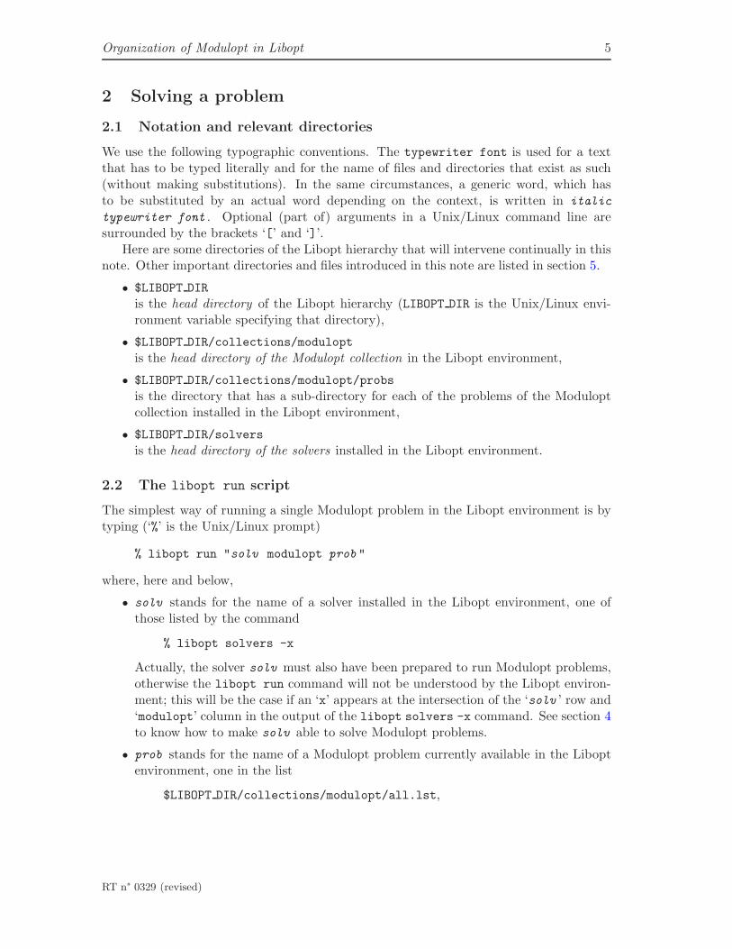
2.2 The libopt run script

The simplest way of running a single Modulopt problem in the Libopt environment is bytyping (‘%’ is the Unix/Linux prompt)

% libopt run "solv modulopt prob "

where, here and below,

• solv stands for the name of a solver installed in the Libopt environment, one ofthose listed by the command

% libopt solvers -x

Actually, the solver solv must also have been prepared to run Modulopt problems,otherwise the libopt run command will not be understood by the Libopt environ-ment; this will be the case if an ‘x’ appears at the intersection of the ‘solv ’ row and‘modulopt’ column in the output of the libopt solvers -x command. See section 4to know how to make solv able to solve Modulopt problems.

• prob stands for the name of a Modulopt problem currently available in the Liboptenvironment, one in the list

$LIBOPT DIR/collections/modulopt/all.lst,


6 J. Ch. Gilbert

The name prob of some problems can be composed, formed of two strings separatedby a dot like in

pnam.pdat

In this case, Libopt only sees the composed name prob = pnam.pdat , but forModulopt, the radical name pnam of the problem is a string used to identify theproblem directory and the data name pdat is a string used to identify one of itsdata sets. Hence, a problem may have several data sets. In the Modulopt collection,the problem pnam is stored in the directory (pnam and prob are identical if there isno dot in the string, i.e., when there is a single data set)

$LIBOPT DIR/collections/modulopt/probs/pnam ,

called the problem directory. How the data sets are built from the string pdat

depends on each problem.

By the libopt run command above, the optimization solver solv is used to solve theModulopt optimization problem prob. Of course solv has to be able to solve a problemwith the features of prob (for example, a solver for unconstrained optimization problemsis unable to solve problems with constraints). The solver solv keeps in the file

$LIBOPT DIR/solvers/solv/modulopt/all.lst

the list of the Modulopt problems that it can structurally solve.See the Libopt manual [4] or the manual page of libopt to learn how to run a group

of problems with a given solver, using a single command line or a file describing what hasto be done.

The directory where the libopt run command given above is typed is called theworking directory. When this is important, the Libopt commands take care that thisdirectory is not in the Libopt hierarchy. If this were the case, there could be a danger ofincurable destruction. Indeed, a command like libopt run generally removes several filesfrom the working directory after a problem has been solved.

2.3 The solv modulopt script

By decoding the directive “solv modulopt prob ”, where prob is the string

pnam [.pdat],

the libopt run command above knows that it has to launch the following script:

$LIBOPT DIR/solvers/solv/modulopt/solv modulopt

with prob in argument. In the standard distribution, solv modulopt is a Perl script,but nothing imposes that such a language be used. Such a script has to be written foreach solver that wants and is able to solve Modulopt problems. Luckily, this script canbe generated from a template (see section 4 for the details). For the while, it is enough toknow that it contains the following main steps.

• The environment variables given on the left in the table below are set the value givenon the right:

INRIA


MODULOPT PROB prob

MODULOPT PNAM pnam

MODULOPT PDAT pdat

WORKING DIR working directory.

These variables can then be used in the scripts and makefiles mentioned below.Actually, the environment variable WORKING DIR is probably useless since all theUnix/Linux commands in the scripts or makefiles are executed from the workingdirectory (there is no change of directory made in them).

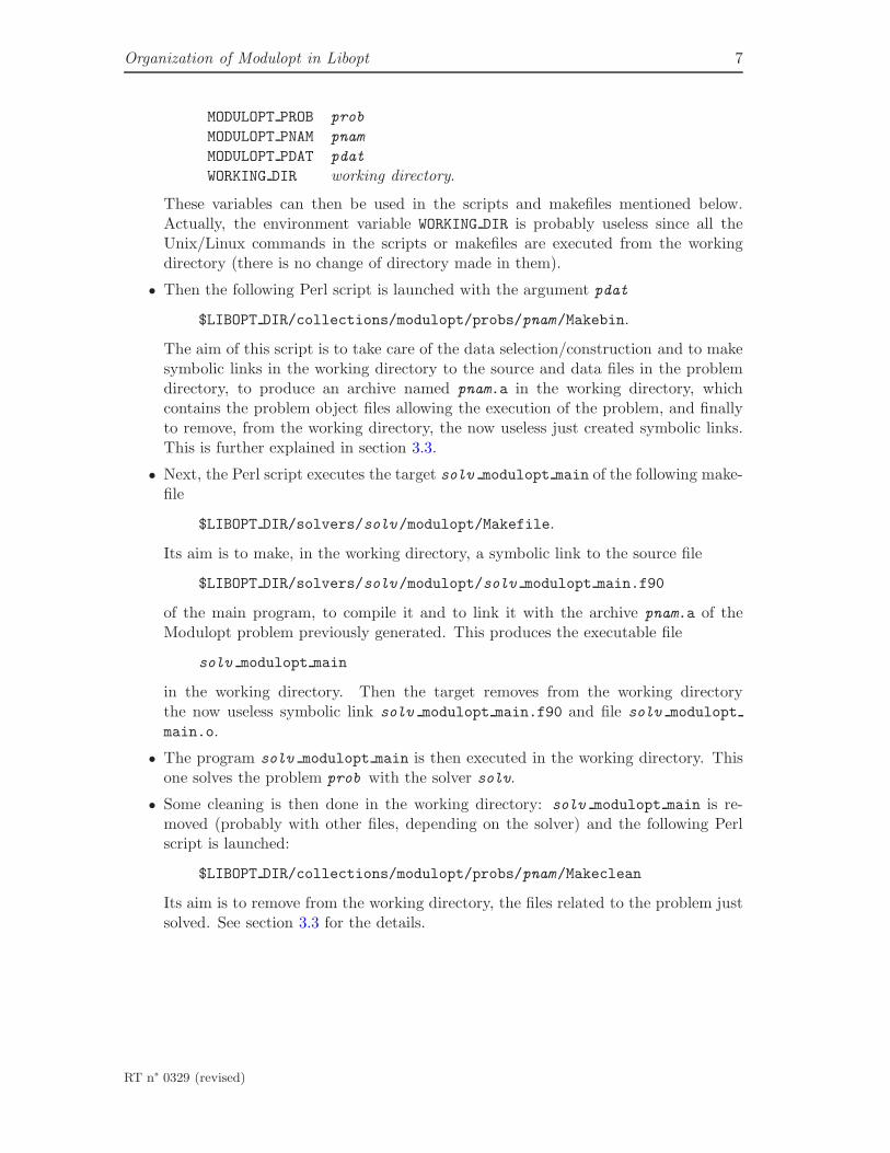
• Then the following Perl script is launched with the argument pdat

$LIBOPT DIR/collections/modulopt/probs/pnam/Makebin.

The aim of this script is to take care of the data selection/construction and to makesymbolic links in the working directory to the source and data files in the problemdirectory, to produce an archive named pnam.a in the working directory, whichcontains the problem object files allowing the execution of the problem, and finallyto remove, from the working directory, the now useless just created symbolic links.This is further explained in section 3.3.

• Next, the Perl script executes the target solv modulopt main of the following make-file

$LIBOPT DIR/solvers/solv/modulopt/Makefile.

Its aim is to make, in the working directory, a symbolic link to the source file

$LIBOPT DIR/solvers/solv/modulopt/solv modulopt main.f90

of the main program, to compile it and to link it with the archive pnam.a of theModulopt problem previously generated. This produces the executable file

solv modulopt main

in the working directory. Then the target removes from the working directorythe now useless symbolic link solv modulopt main.f90 and file solv modulopt

main.o.

• The program solv modulopt main is then executed in the working directory. Thisone solves the problem prob with the solver solv.

• Some cleaning is then done in the working directory: solv modulopt main is re-moved (probably with other files, depending on the solver) and the following Perlscript is launched:

$LIBOPT DIR/collections/modulopt/probs/pnam/Makeclean

Its aim is to remove from the working directory, the files related to the problem justsolved. See section 3.3 for the details.


8 J. Ch. Gilbert

3 Introducing/removing a problem in/from the collection

3.1 The libopt addproblem command

Suppose we want to add a new problem named

prob or pnam [.pdat]

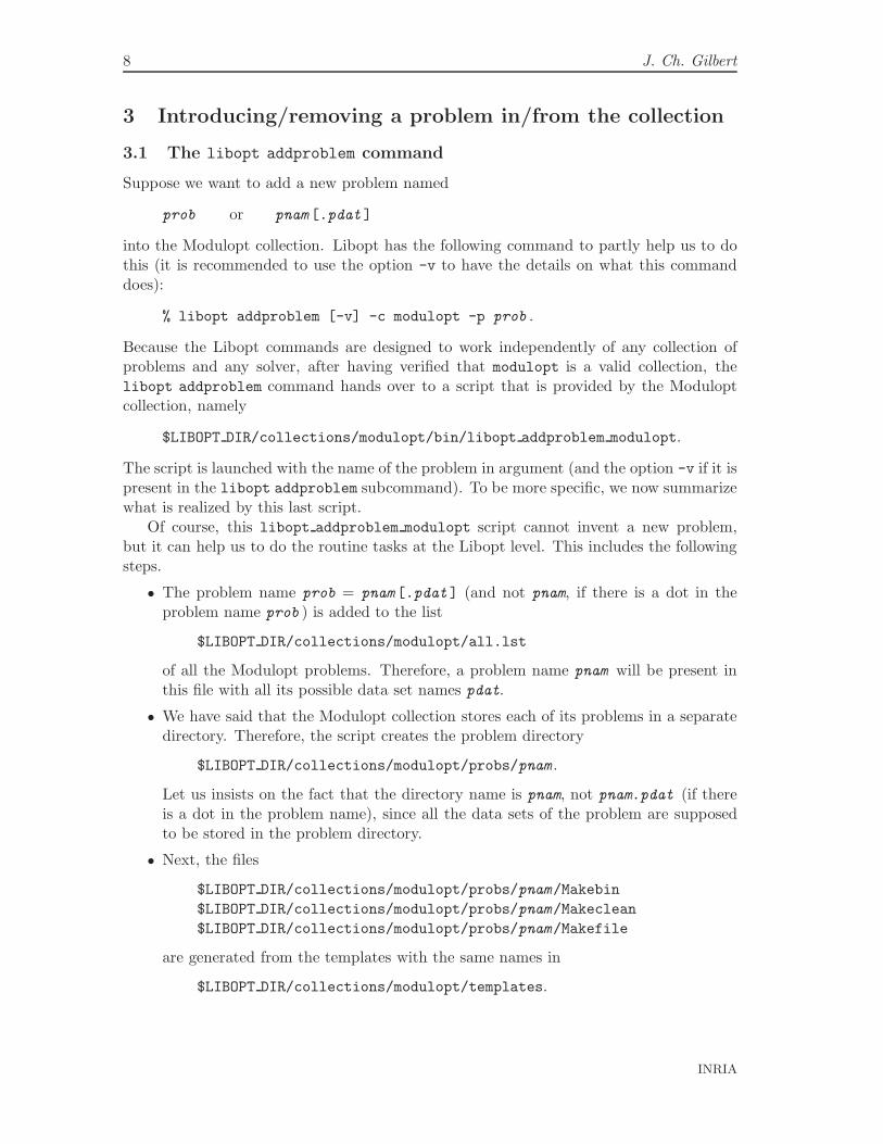
into the Modulopt collection. Libopt has the following command to partly help us to dothis (it is recommended to use the option -v to have the details on what this commanddoes):

% libopt addproblem [-v] -c modulopt -p prob .

Because the Libopt commands are designed to work independently of any collection ofproblems and any solver, after having verified that modulopt is a valid collection, thelibopt addproblem command hands over to a script that is provided by the Moduloptcollection, namely

$LIBOPT DIR/collections/modulopt/bin/libopt addproblem modulopt.

The script is launched with the name of the problem in argument (and the option -v if it ispresent in the libopt addproblem subcommand). To be more specific, we now summarizewhat is realized by this last script.

Of course, this libopt addproblem modulopt script cannot invent a new problem,but it can help us to do the routine tasks at the Libopt level. This includes the followingsteps.

• The problem name prob = pnam [.pdat] (and not pnam, if there is a dot in theproblem name prob ) is added to the list

$LIBOPT DIR/collections/modulopt/all.lst

of all the Modulopt problems. Therefore, a problem name pnam will be present inthis file with all its possible data set names pdat.

• We have said that the Modulopt collection stores each of its problems in a separatedirectory. Therefore, the script creates the problem directory

$LIBOPT DIR/collections/modulopt/probs/pnam .

Let us insists on the fact that the directory name is pnam, not pnam.pdat (if thereis a dot in the problem name), since all the data sets of the problem are supposedto be stored in the problem directory.

• Next, the files

$LIBOPT DIR/collections/modulopt/probs/pnam/Makebin

$LIBOPT DIR/collections/modulopt/probs/pnam/Makeclean

$LIBOPT DIR/collections/modulopt/probs/pnam/Makefile

are generated from the templates with the same names in

$LIBOPT DIR/collections/modulopt/templates.

INRIA


The role of these files is explained in section 3.3. To generate them from the tem-plates, libopt addproblem modulopt uses the file

$LIBOPT DIR/collections/modulopt/probs/pnam/links.lst,$LIBOPT DIR/collections/modulopt/probs/pnam/unlinks.lst.

The file links.lst specifies the names of the files in the problem directory that mustbe symbolically linked to files in the working directory when the problem is executed;while the file unlinks.lst specifies the files related to the problem prob that mustbe deleted from the working directory after the problem prob as been solved. Ifthe file links.lst (resp. unlinks.lst) does not exist, Makebin (resp. Makeclean)is not generated. This is necessary the case the first time libopt addproblem isrun to introduce the problem; hence rerun the command after having introduced thepossibly empty files links.lst and unlinks.lst. This second run will completethe installation of the problem, without destroying what has already been done bythe first run.

The libopt addproblem command also lists what has to be done manually to completethe installation of the prob problem into Modulopt. This includes one or more of thefollowing items.

• If this is appropriate, add the name prob to other lists of problems

$LIBOPT DIR/collections/modulopt/*.lst,

such as the one related to unconstrained problems unc.lst, quadratic problemsquad.lst, etc, as well as the list of typical problems of the Modulopt collectiondefault.lst. These are ascii files. An alpha-numeric order has been adopted, butthis feature is not taken into account by the Libopt scripts. Comments are possible;they start from the character ‘#’ up to the end of the line.

• If a solver called solv is able to solve a problem like prob, it may be appropriate toadd the name prob in one or more files among

$LIBOPT DIR/solvers/solv/modulopt/*.lst.

This assumes that the directory $LIBOPT DIR/solvers/solv/modulopt exists andthat the solver has been prepared to solve problems from the Modulopt collection(see section 4 to know how to do this).

• Put in the directory

$LIBOPT DIR/collections/modulopt/probs/prob ,

all the files that define the problem prob : source files, header files (if appropriate),and data files (if appropriate). This is further described in section 3.2 below.

• Make it clear in

$LIBOPT DIR/collections/modulopt/probs/prob/Makebin,

how to generate the data set from the string pdat and how the main program solv

modulopt main can have access to this data set. Examples are given in some problemdirectories. See also section 3.3.


10 J. Ch. Gilbert

3.2 The subroutines defining a Modulopt problem

In principle, the problem can be described in any compiled language, provided the binaryfiles can be gathered into an archive. Below, we assume that the problem is written inFortran 95.

The problem-independent makefile

$LIBOPT DIR/solvers/solv/modulopt/Makefile

assumes that the problem to execute is in the archive prob.a in the working directory.On the other hand, the problem-independent main program solv modulopt main assumesthat the archive prob.a contains seven subroutines: dimopt, initopt, simulopt, postopt,inprodopt, ctonbopt, and ctcabopt, which are described below.

In the description of the subroutine arguments, an argument tagged with (I) meansthat it is an input variable, which has to be initialized before calling the subroutine; anargument tagged with (O) means that it is an output variable, which only has a meaningon return from the subroutine; and an argument tagged with (IO) is an input-output

argument, which has to be initialized and which has a meaning after the call to thesubroutine. Arguments of the type (O) and (IO) are generally modified by the subroutineand therefore should not be Fortran constants!

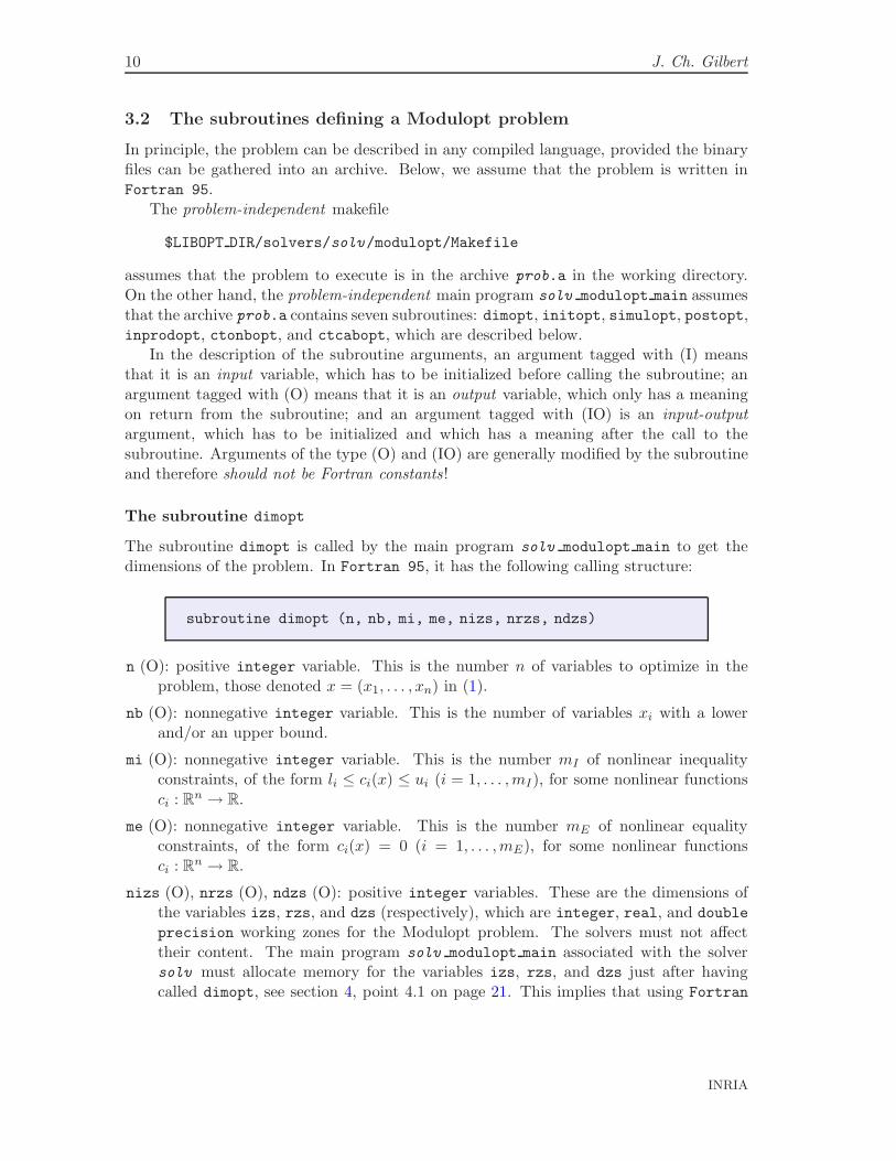
The subroutine dimopt

The subroutine dimopt is called by the main program solv modulopt main to get thedimensions of the problem. In Fortran 95, it has the following calling structure:

subroutine dimopt (n, nb, mi, me, nizs, nrzs, ndzs)

n (O): positive integer variable. This is the number n of variables to optimize in theproblem, those denoted x = (x1, . . . , xn) in (1).

nb (O): nonnegative integer variable. This is the number of variables xi with a lowerand/or an upper bound.

mi (O): nonnegative integer variable. This is the number mI of nonlinear inequalityconstraints, of the form li ≤ ci(x) ≤ ui (i = 1, . . . ,mI), for some nonlinear functionsci : R

n → R.

me (O): nonnegative integer variable. This is the number mE of nonlinear equalityconstraints, of the form ci(x) = 0 (i = 1, . . . ,mE), for some nonlinear functionsci : R

n → R.

nizs (O), nrzs (O), ndzs (O): positive integer variables. These are the dimensions ofthe variables izs, rzs, and dzs (respectively), which are integer, real, and double

precision working zones for the Modulopt problem. The solvers must not affecttheir content. The main program solv modulopt main associated with the solversolv must allocate memory for the variables izs, rzs, and dzs just after havingcalled dimopt, see section 4, point 4.1 on page 21. This implies that using Fortran

INRIA


77 is not an appropriate language for writing the main program solv modulopt

main. Note that the value of nizs, nrzs, and ndzs can be zero.

The subroutine initopt

The subroutine initopt is called to initialize the problem. In Fortran 95, it has thefollowing calling structure:

subroutine initopt (pname, n, mi, me, x, lx, ux, dxmin, li, ui,

dcimin, infb, tolopt, simcap, info, izs,

rzs, dzs)

pname (O): character string of length 132, giving the name of the problem.

n (I), mi (I), me (I): dimensions of the problem. Their meaning is given in the descriptionof dimopt.

x (O): double precision array of dimension n, providing a starting point for the opti-mization solver.

lx (O), ux (O): double precision array of dimension n, providing the bounds on thevariable x, if any. If the variables are not subject to bounds (nb is zero on returnfrom dimopt), these variables will not be set and can be ddeclared in the callingprogram as scalars; if some variables are subject to bounds their must be declared inthe calling program with the dimension n.

If the variables are subject to bounds, their values xi are required to satisfy lx(i) ≤xi ≤ ux(i), for i = 1, . . . , n. The lower (resp. upper) bound lx(i) (resp. ux(i)) is setto -infb (resp. infb) is the bound does not exist; see below for the meaning of infb.

dxmin (O): double precision variable, providing the resolution in x for the l∞ norm:two points whose distance in R

n for the sup-norm is less than dxmin can be consideredas indistinguishable. This data can be used in line-search or trust-region. It is alsouseful to detect bounds that are active up to that precision.

li (O), ui (O): double precision array of dimension mi := mI , providing the boundson the constraint values cI(x). In other words, ci(x) is required to satisfy li(i) ≤ci(x) ≤ ui(i), for i = 1, . . . ,mI .

dcimin (O): double precision variable, providing the resolution in cI for the l∞ norm:two inequality constraint values whose distance in R

mI for the sup-norm is less thandcimin can be considered as indistinguishable. This data can be useful to detectinequality constraints that are active up to that precision.

infb (O): double precision variable, specifying what is the infinite value for the boundson x and cI(x). In other words, when lx(i) ≤ −infb (resp. li(i) ≤ −infb), thereis no lower bound on xi (resp. ci(x)). A similar convention is adopted for the upperbounds.


12 J. Ch. Gilbert

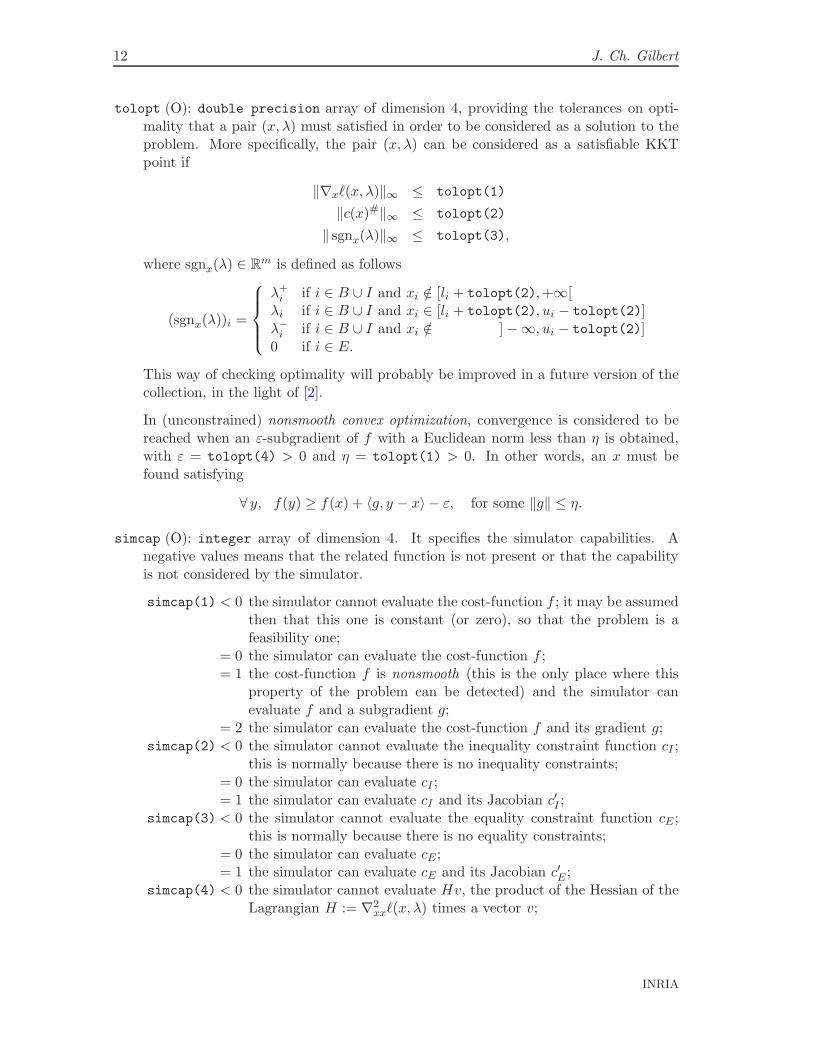
tolopt (O): double precision array of dimension 4, providing the tolerances on opti-mality that a pair (x, λ) must satisfied in order to be considered as a solution to theproblem. More specifically, the pair (x, λ) can be considered as a satisfiable KKTpoint if

‖∇xℓ(x, λ)‖∞ ≤ tolopt(1)

‖c(x)#‖∞ ≤ tolopt(2)

‖ sgnx(λ)‖∞ ≤ tolopt(3),

where sgnx(λ) ∈ Rm is defined as follows

(sgnx(λ))i =

λ+i if i ∈ B ∪ I and xi /∈ [li + tolopt(2),+∞[

λi if i ∈ B ∪ I and xi ∈ [li + tolopt(2), ui − tolopt(2)]λ−

i if i ∈ B ∪ I and xi /∈ ] −∞, ui − tolopt(2)]0 if i ∈ E.

This way of checking optimality will probably be improved in a future version of thecollection, in the light of [2].

In (unconstrained) nonsmooth convex optimization, convergence is considered to bereached when an ε-subgradient of f with a Euclidean norm less than η is obtained,with ε = tolopt(4) > 0 and η = tolopt(1) > 0. In other words, an x must befound satisfying

∀ y, f(y) ≥ f(x) + 〈g, y − x〉 − ε, for some ‖g‖ ≤ η.

simcap (O): integer array of dimension 4. It specifies the simulator capabilities. Anegative values means that the related function is not present or that the capabilityis not considered by the simulator.

simcap(1) < 0 the simulator cannot evaluate the cost-function f ; it may be assumedthen that this one is constant (or zero), so that the problem is afeasibility one;

= 0 the simulator can evaluate the cost-function f ;= 1 the cost-function f is nonsmooth (this is the only place where this

property of the problem can be detected) and the simulator canevaluate f and a subgradient g;

= 2 the simulator can evaluate the cost-function f and its gradient g;simcap(2) < 0 the simulator cannot evaluate the inequality constraint function cI ;

this is normally because there is no inequality constraints;= 0 the simulator can evaluate cI ;= 1 the simulator can evaluate cI and its Jacobian c′I ;

simcap(3) < 0 the simulator cannot evaluate the equality constraint function cE ;this is normally because there is no equality constraints;

= 0 the simulator can evaluate cE ;= 1 the simulator can evaluate cE and its Jacobian c′E ;

simcap(4) < 0 the simulator cannot evaluate Hv, the product of the Hessian of theLagrangian H := ∇2

xxℓ(x, λ) times a vector v;

INRIA


= 1 the simulator can evaluate a product Hv;= 2 the simulator can evaluate the H.

info (O): integer variable. If negative (< 0), solv modulopt main should consider thatthe initialization of the problem by initopt has failed and should stop.

izs, rzs, dzs (O): integer, real, and double precision arrays that initopt shouldinitialize. These variables are made available to the Modulopt problem. Their dimen-sions have been provided on return from dimopt and they should have been allocatedby the main program solv modulopt main associated with some code solv.

The subroutine simulopt

The subroutine simulopt is the simulator of the problem. It can be called by solv

modulopt main, before calling solv. It is also called by the latter to have information(function and their derivatives) on the problem to solve. In Fortran 95, it has the fol-lowing calling structure:

subroutine simulopt (indic, n, mi, me, x, lm, f, ci, ce, g, ai,

ae, v, hlv, hl, izs, rzs, dzs)

indic (IO): integer variable monitoring the communication between the solver and thesimulator. The simulator simulopt recognizes the following values of indic.

= 1: The simulator can do anything except changing the value of the arguments ofsimulopt. Typically it prints some information on the screen, in a file, or ona plotter. Some solver calls the simulator with this value of indic at eachiteration.

= 2: The simulator is asked to compute the value of the functions f = f(x) ∈ R (costfunction), ci = cI(x) ∈ R

mI (inequality constraints), and ce = cE(x) ∈ RmE

(equality constraints) at a given point x.= 3: The simulator is asked to compute g = ∇f(x) ∈ R

n (gradient of f at x for theEuclidean scalar product), ai = c′I(x) (mI ×n Jacobian matrix of cI at x, hencethe (i, j) entry of ai must be the partial derivative ∂ci/∂xj evaluated at x), andae = c′E(x) (mE × n Jacobian matrix of cE at x).

= 4: The simulator is asked to compute f = f(x), ci = cI(x), and ce = cE(x) ata given point x, as well as the gradient g = ∇f(x) ∈ R

n, ai = c′I(x), andae = c′E(x).

= 5: The simulator is asked to compute the Hessian of the Lagrangian H := ∇2xxℓ(x, λ)

at the point (x, λ).

On the other hand, the simulator simulopt can also send a message to the solver, bygiving to indic one of the following values.

≥ 0: normal call; the required computation has been done.


14 J. Ch. Gilbert

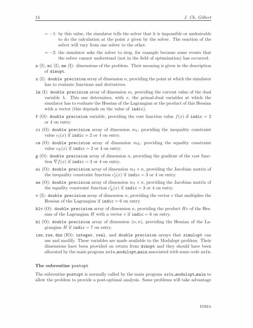
= −1: by this value, the simulator tells the solver that it is impossible or undesirableto do the calculation at the point x given by the solver. The reaction of thesolver will vary from one solver to the other.

= −2: the simulator asks the solver to stop, for example because some events thatthe solver cannot understand (not in the field of optimization) has occurred.


x (I): double precision array of dimension n, providing the point at which the simulatorhas to evaluate functions and derivatives.

lm (I): double precision array of dimension m, providing the current value of the dualvariable λ. This one determines, with x, the primal-dual variables at which thesimulator has to evaluate the Hessian of the Lagrangian or the product of this Hessianwith a vector (this depends on the value of indic).

f (O): double precision variable, providing the cost function value f(x) if indic = 2or 4 on entry.

ci (O): double precision array of dimension mI , providing the inequality constraintvalue cI(x) if indic = 2 or 4 on entry.

ce (O): double precision array of dimension mE, providing the equality constraintvalue cE(x) if indic = 2 or 4 on entry.

g (O): double precision array of dimension n, providing the gradient of the cost func-tion ∇f(x) if indic = 3 or 4 on entry.

ai (O): double precision array of dimension mI × n, providing the Jacobian matrix ofthe inequality constraint function c′I(x) if indic = 3 or 4 on entry.

ae (O): double precision array of dimension mI × n, providing the Jacobian matrix ofthe equality constraint function c′E(x) if indic = 3 or 4 on entry.

v (I): double precision array of dimension n, providing the vector v that multiplies theHessian of the Lagrangian if indic = 6 on entry.

hlv (O): double precision array of dimension n, providing the product Hv of the Hes-sian of the Lagrangian H with a vector v if indic = 6 on entry.

hl (O): double precision array of dimension (n, n), providing the Hessian of the La-grangian H if indic = 7 on entry.

izs, rzs, dzs (IO): integer, real, and double precision arrays that simulopt canuse and modify. These variables are made available to the Modulopt problem. Theirdimensions have been provided on return from dimopt and they should have beenallocated by the main program solv modulopt main associated with some code solv.

The subroutine postopt

The subroutine postopt is normally called by the main program solv modulopt main toallow the problem to provide a post-optimal analysis. Some problems will take advantage

INRIA


of this opportunity, but most of them won’t (they will provide a subroutine with en emptybody). The most trivial operation that can be done in this subroutine is to print thesolution on the screen. Another possibility is to check second order optimality. Theflexibility offered by this subroutine will allow the user of libopt to make other job thancomparing the effect of using various solvers on his/her problem.

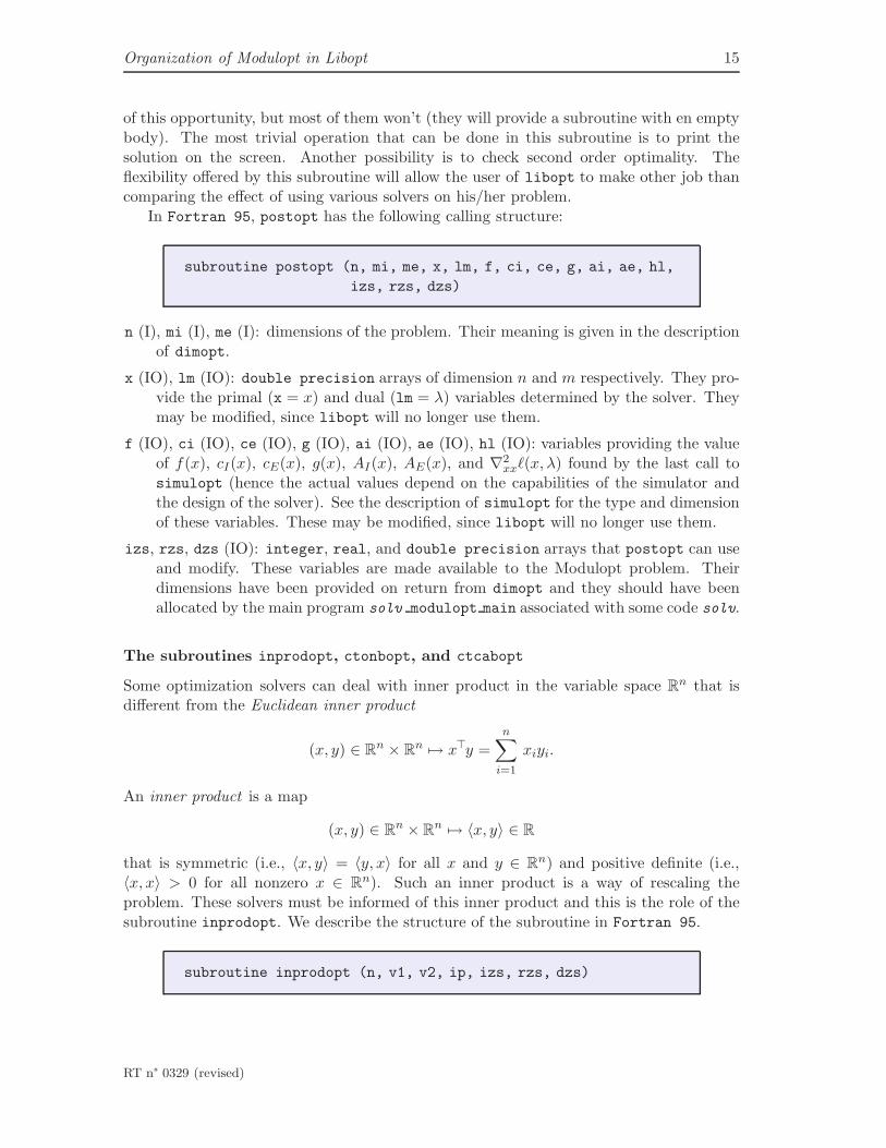
In Fortran 95, postopt has the following calling structure:

subroutine postopt (n, mi, me, x, lm, f, ci, ce, g, ai, ae, hl,

izs, rzs, dzs)


x (IO), lm (IO): double precision arrays of dimension n and m respectively. They pro-vide the primal (x = x) and dual (lm = λ) variables determined by the solver. Theymay be modified, since libopt will no longer use them.

f (IO), ci (IO), ce (IO), g (IO), ai (IO), ae (IO), hl (IO): variables providing the valueof f(x), cI(x), cE(x), g(x), AI(x), AE(x), and ∇2

xxℓ(x, λ) found by the last call tosimulopt (hence the actual values depend on the capabilities of the simulator andthe design of the solver). See the description of simulopt for the type and dimensionof these variables. These may be modified, since libopt will no longer use them.

izs, rzs, dzs (IO): integer, real, and double precision arrays that postopt can useand modify. These variables are made available to the Modulopt problem. Theirdimensions have been provided on return from dimopt and they should have beenallocated by the main program solv modulopt main associated with some code solv.

The subroutines inprodopt, ctonbopt, and ctcabopt

Some optimization solvers can deal with inner product in the variable space Rn that is

different from the Euclidean inner product

(x, y) ∈ Rn × R

n 7→ x⊤y =n

∑

i=1

xiyi.

An inner product is a map

(x, y) ∈ Rn × R

n 7→ 〈x, y〉 ∈ R

that is symmetric (i.e., 〈x, y〉 = 〈y, x〉 for all x and y ∈ Rn) and positive definite (i.e.,

〈x, x〉 > 0 for all nonzero x ∈ Rn). Such an inner product is a way of rescaling the

problem. These solvers must be informed of this inner product and this is the role of thesubroutine inprodopt. We describe the structure of the subroutine in Fortran 95.

subroutine inprodopt (n, v1, v2, ip, izs, rzs, dzs)


16 J. Ch. Gilbert

n (I): dimension of the vectors whose inner product is going to be taken.

v1 (I), v2 (I): double precision arrays of dimension n. These are the vectors whoseinner product is desired.

ip (O): double precision variable representing the inner product of v1 and v2.

izs, rzs, dzs (IO): integer, real, and double precision arrays that postopt can useand modify. These variables are made available to the Modulopt problem. Theirdimensions have been provided on return from dimopt and they should have beenallocated by the main program solv modulopt main associated with some code solv.

Some unconstrained optimization solvers not only need the inner product subroutineinprodopt but also subroutines that make a change of coordinates from the canonical

orthogonal basis of Rn to some orthogonal basis for the inner product 〈·, ·〉. The canonical

orthogonal basis of Rn is the set of vectors {ei}n

i=1, where the jth component of ei is equalto δij (the Kronecker symbol, which is one when i = j and zero otherwise). If a vector iswritten

∑

i xiei in the canonical basis and

∑

i yiei in the considered orthogonal basis, the

subroutine ctonbopt gives the coordinates y := (y1, . . . , yn) from x := (x1, . . . , xn) andthe subroutine ctcabopt gives the coordinates x from y.

For example, suppose that〈u, v〉 = u⊤M⊤Mv,

where M is a nonsingular n × n matrix, such that a linear system with the matrix Mis easy to solve (for example M could be triangular). One can take ei = M−1ei, for1 ≤ i ≤ n, since then 〈ei, ej〉 = (ei)⊤M⊤Mej = (ei)⊤ej = δij . Knowing the coordinatesx := (x1, . . . , xn) of a vector in the canonical basis, its coordinates y := (y1, . . . , yn) in thebasis {ei}n

i=1 can be computed by

yj = 〈∑

i

xiei, ej〉 =

∑

i

xi〈ei,M−1ej〉 =

∑

i

xi(ei)⊤M⊤ej = (Mx)j .

We have shown that y = Mx. In that example, the subroutine ctonbopt will computey = Mx knowing x, while the subroutine ctcabopt will compute x = M−1y knowing y.

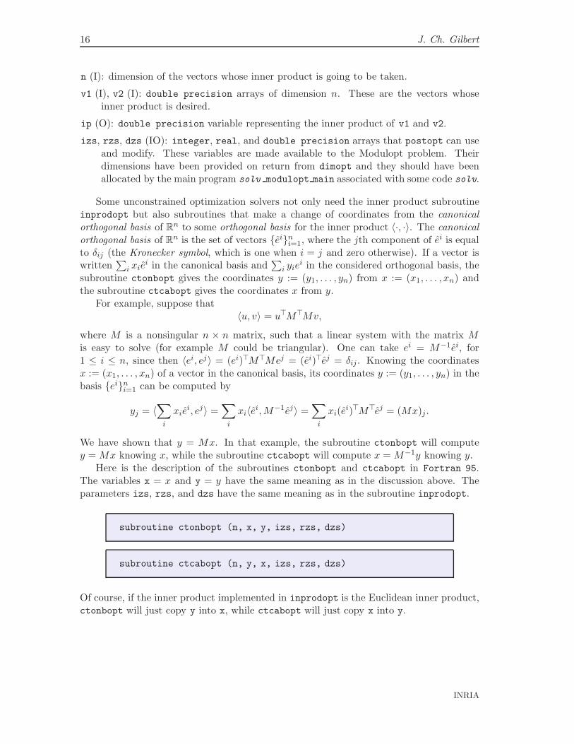
Here is the description of the subroutines ctonbopt and ctcabopt in Fortran 95.The variables x = x and y = y have the same meaning as in the discussion above. Theparameters izs, rzs, and dzs have the same meaning as in the subroutine inprodopt.

subroutine ctonbopt (n, x, y, izs, rzs, dzs)

subroutine ctcabopt (n, y, x, izs, rzs, dzs)

Of course, if the inner product implemented in inprodopt is the Euclidean inner product,ctonbopt will just copy y into x, while ctcabopt will just copy x into y.

INRIA


3.3 The files describing how to run a Modulopt problem

A problem, whose name is pnam [.pdat], can be stored in an arbitrary manner in itsdirectory

$LIBOPT DIR/collections/modulopt/probs/pnam .

Of course, the Libopt environment must be told how to make the information contained inthat directory available to the solvers that want to solve the problem. As far as Libopt isconcerned, three files (two scripts and a makefile) located in the problem directory suffice:Makebin, Makeclean, and Makefile. These files have been encountered in sections 2.3and 3.1 and their role and contents is fully described in this section. Recall from section 3.1that these three files can be largely automatically generated, using the templates with thesame name in

$LIBOPT DIR/collections/modulopt/templates.

This file generation is done by the script libopt addproblem modulopt, itself called bythe libopt addproblem command. Sometimes, however, these files must be customized,so that understanding what they do is certainly useful.

The script Makebin has two goals: it takes care of the data selection or constructionand, thanks to Makefile, it produces in the working directory an archive, named prob.a,which contains all the binaries related to the problem. On the other hand, the scriptMakeclean removes from the working directory the files that have been generated before,during, and/or after the problem prob is solved.

One must keep in mind that Makebin, Makeclean, and Makefile must be designed insuch a way that no file is generated in the problem directory. This is to make sure thatseveral users can use the Libopt environment at the same time.

The script Makebin and the Makefile

A solv modulopt script can invoke Makebin through the command

% Makebin [-g] [-k] [-t] [-v] [pdat]

where the option -g asks to put in prob.a binaries with symbolic debug information, theoption -k asks to keep any generated file in the working directory (files that become uselessat a certain stage of the operations are not removed), the option -t asks for a test runningmode, meaning that commands are displayed but not executed, the option -v asks for averbose execution of the script. The script contains the following steps.

• The argument pdat (if any) is normally used to select or construct the data filescorresponding to the problem pnam[.pdat]. If it is a selection of data files, sym-bolic links to the relevant files will be created in the working directory. If it is aconstruction of data files, these will be placed in the working directory, not in theproblem directory in order to preserve the integrity of the Libopt directory contents.

• Next, symbolic links are defined in the working directory towards files that are usefulfor running the problem. As already said in section 3.1, to generate Makebin from atemplate, the script libopt addproblem modulopt reads the list


18 J. Ch. Gilbert

$LIBOPT DIR/collections/modulopt/probs/pnam/links.lst

to get the files that need to be linked.

• In the last step, Makebin runs the makefile

$LIBOPT DIR/collections/modulopt/probs/pnam/Makefile

with prob in argument (the target) and with appropriate flags inherited from those ofMakebin. The role of this makefile is to build the archive prob.a with all the binariesrelated to the problem, including the object files corresponding to the subroutinesdescribed in section 3.2. Makefile uses the environment variable LIBOPT PLAT totune the binaries to the correct platform.

The script Makeclean

After having solved prob with some solver, the libopt run command removes the filesthat have been generated in the working directory (unless the option -k asks to keepthem). Part of these files are directly linked to the problem (the data files, for example).The script Makeclean is there to tell the solv modulopt script which files to remove. Itcan be called by

% Makeclean [-t] [-v]

where the options -t and -v have the same meaning as for the script Makebin.As already said in section 3.1, to generate Makeclean from a template, the script

libopt addproblem modulopt reads the list

$LIBOPT DIR/collections/modulopt/probs/pnam/unlinks.lst

to get the files that need to be removed.

3.4 The libopt rmproblem command

In Libopt, the counterpart of the command that can add a problem to a collection (liboptaddproblem, see section 3.1) is the libopt rmproblem command, which can be used toremove a problem from a collection. For the Modulopt collection, it reads

% libopt rmproblem [-v] -c modulopt -p prob ,

where prob is the name of the problem that has to be removed (the form pnam [.pdat]

of the problem name can be used instead).Because the Libopt commands are designed to work independently of any collection

of problems and any solver, after having verified that modulopt is a valid collection, thelibopt rmproblem command hands over to a script that is provided by the Moduloptcollection, namely

$LIBOPT DIR/collections/modulopt/bin/libopt rmproblem modulopt.

INRIA


The script is launched with the name of the problem in argument (and the option -v if itis present in the libopt rmproblem command).

A problem can contain a large amount of programs and data. By removing a problem,the script libopt rmproblem modulopt will not remove that information, but will makeit concealed from Libopt. It is the responsibility of the designer of the collection to decidewhether the directory containing the problem data really needs to be removed. Actually,libopt rmproblem modulopt essentially modifies lists of problems and, to be friendly,enumerates the possible modifications that must be made by hand.

Let us summarize what is realized by this script libopt rmproblem modulopt.

• The problem name pnam[.pdat ] (and not pnam, if there is a dot in the problemname prob ) is removed from the list

$LIBOPT DIR/collections/modulopt/all.lst

of all the Modulopt problems.

• It is then asked whether prob has to be removed from all, some, or none of the otherlists (those files with the suffix .lst) in the directory

$LIBOPT DIR/collections/modulopt.

The script acts according to the answer given by the user.

• Next, it is asked whether prob has to be removed from all, some, or none of the listsin the existing directories

$LIBOPT DIR/solvers/solv/modulopt,

where solv is any of the solvers installed in the environment. The script actsaccording to the answer given by the user.

The script concludes by enumerating what has to be done manually to complete theremoval of the prob problem from the Modulopt collection.

4 Making a solver able to solve Modulopt problems

In this section, we consider the case when it is desirable to make a solver of optimizationproblems, installed in the Libopt environment, able to solve problems from the Moduloptcollection. Let

solv

be the name of the considered solver. We refer the reader to the Libopt manual [4] tolearn how to install the solver solv in Libopt if this one is not already present in theenvironment.

In the Libopt terminology, building the interface between solv and Modulopt is calledactivating the (solv, modulopt) cell; the word cell refers to an element of the {solvers} ×{collections} Cartesian product. The interface is the set of scripts and programs thatallows solv to solve Modulopt problems. These pieces of software are placed in theinterface directory


20 J. Ch. Gilbert

$LIBOPT DIR/solvers/solv/modulopt.

Luckily, there is a command that takes in charge part of the job:

% libopt addcell -s solv -c modulopt [-v]

where the flag -s prefixes the solver name solv, the flag -c prefixes the collection namemodulopt, and the option -v asks for a verbose running mode (recommended). In additionto doing some verifications, in order to check and maintain the consistency of the Liboptenvironment, the libopt addcell command completes various lists (hidden to the user)and fills in the interface directory.

An important goal of the libopt addcell command is to generate the solv modulopt

script in the interface directory. Since this script is linked to the Modulopt collection, itcannot be generated at the Libopt level. Instead, libopt addcell hands over to thegenerating script

$LIBOPT DIR/collections/modulopt/bin/libopt addcell modulopt

which is provided with the Modulopt collection. This one generates solv modulopt bytransforming the template

$LIBOPT DIR/collections/modulopt/templates/SOLV modulopt,

essentially replacing the occurrences of <SOLV> (resp. <COLL>) by solv (resp. modulopt)and adding Perl lines to remove the files listed by the outfiles directive mentioned inthe file

$LIBOPT DIR/solvers/solv/doc/solv features.

It is likely that nothing will have to be modified in the solv modulopt script to make itwork as desired. It is wise to check it, however, recalling that its required contents hasbeen given in section 2.3.

The libopt addcell command also specifies what needs to be done by hand. Theseincludes the following points.

1. Fill in the files

$LIBOPT DIR/solvers/solv/modulopt/all.lst

$LIBOPT DIR/solvers/solv/modulopt/default.lst.

• The first file (all.lst) must list the problems from the Modulopt collection thatsolv is able to solve or, more precisely, those for which it has been conceived. It cancontain comments, which start with the ‘#’ character and go up to the end of theline. The easiest way of doing this is to start with a copy of the file

$LIBOPT DIR/collections/modulopt/all.lst,

which lists all the Modulopt problems, and to remove from the copied file thoseproblems that do not have the structure expected by solv. For example, if solv is asolver of unconstrained optimization problems, remove from the copied file all.lst,all the problems with constraints. The features of the Modulopt problems are oftenspecified by comments in the file

INRIA


$LIBOPT DIR/collections/modulopt/all.lst.

Note that other lists exist in the directory $LIBOPT DIR/collections/modulopt,which might be more appropriate to start with than the list all.lst.

• The second file above (default.lst) can contain any subset of the problems listedin the first file (all.lst). This file is used as the default subcollection when no listis specified in the libopt run command. Therefore, it is often a symbolic link to thefirst file all.lst, obtained using the Unix/Linux command

ln -s all.lst default.lst

in the directory $LIBOPT DIR/collections/modulopt.

2. Create the main program

$LIBOPT DIR/solvers/solv/modulopt/solv modulopt main.f90.

This program is very solver dependent and is, with the next step to which it is linked,the most difficult task to realize. It is the main program that will be linked withthe subroutines describing the problem from the Modulopt problem selected by thelibopt run command, those in the archive prob.a (if the selected problem is prob,see section 3.3). The language used to write this main program is arbitrary, providedit (or its object form generated by some compiler) can be linked with the object filesin prob.a.

If Fortran 90/95 is the adopted language, the easiest way to proceed is to copy andrename the file

$LIBOPT DIR/solvers/sqppro/modulopt/sqppro modulopt main.f90

into the file

$LIBOPT DIR/solvers/solv/modulopt/solv modulopt main.f90.

Since this main program is very solver dependent, its part dealing with the solver willhave to be thoroughly modified. Let us describe the structure of the program.

2.1. After the declaration of variables, the program calls the subroutine dimopt toget the dimensions of the Modulopt problem that will be selected by the libopt

run command. These dimensions are then used to allocate dimension dependentvariables, including izs, rzs, and dzs.

2.2. The problem data are then obtained by calling the subroutine initopt. This isthe good spot to verify that the features of the problem are compatible with thesolver capabilities, using the variable simcap.

2.3. Some optimization solver requires that the simulator be called before launching theoptimization. In this case, this is the good spot for doing so, by calling simulopt.

2.4. Next, the program calls the optimization solver solv, after having initialized itsarguments and opened relevant files.

2.5. Once the optimization has been completed, it is important to write the libopt

line, which summarizes the performance of the solver solv on the currently solvedModulopt problem. See the Libopt manual [4] or the libopt man page.


22 J. Ch. Gilbert

2.6. It is nice to let the problem do its post-optimal analysis (if any) by finally callingpostopt.

Note that a particular solver usually requires a simulator with another structure thanthe one of simulopt. Therefore an interface between simulopt and the simulatorrequired by solv should be written and placed in the file solv modulopt main.f90.

3. Create the makefile

$LIBOPT DIR/solvers/solv/modulopt/Makefile.

The aim of this makefile is to tell the Libopt environment how to link the solver binarywith the object files describing the Modulopt problem selected by the libopt run

command. If the latter is prob, the corresponding object files will be at link time inthe working directory in the archive prob.a (see section 3.2). The easiest way of doingthis is to start with an existing makefile, like

$LIBOPT DIR/solvers/sqppro/modulopt/Makefile.

This one will be copied and renamed into the file

$LIBOPT DIR/solvers/solv/modulopt/Makefile

and then modified.

You can now try the command

libopt run "solv modulopt prob" -v

where the option -v (verbose) is used to get detailed comments from the Libopt scripts,which then tell what they actually do. The flag -t (test mode) can be used instead, if youwant to see what the scripts would do without asking them to do it.

5 Directories and files

In this section, we list some important directories and files encountered in this note. Recallthat LIBOPT DIR is the environment variable that specifies the head directory of the Libopthierarchy. Below, solv is the generic name of a particular solver known to the Liboptenvironment.

• $LIBOPT DIR/collections:directory of the collections of problems the Libopt environment can deal with.

• $LIBOPT DIR/collections/.collections.lst:list of collections known to and installed into Libopt.

• $LIBOPT DIR/collections/modulopt:head directory of the Modulopt collection in the Libopt environment.

• $LIBOPT DIR/collections/modulopt/all.lst:list of all the problems of the Modulopt collection.

• $LIBOPT DIR/collections/modulopt/bin;contains scripts that help some libopt commands to add a (solv, modulopt) cell andto add/remove a problem to/from the Modulopt collection.

INRIA


• $LIBOPT DIR/collections/modulopt/probs:directory containing one sub-directory for each problem of the Modulopt collection.

• $LIBOPT DIR/collections/modulopt/templates;contains scripts and makefiles that help some libopt commands to add a (solv,modulopt) cell and to add a problem to the Modulopt collection.

• $LIBOPT DIR/solvers:head directory of the solvers the Libopt environment can deal with.

• $LIBOPT DIR/solvers/.solvers.lst:list of solvers known to and installed into Libopt.

• $LIBOPT DIR/solvers/solv/.collections.lst:list of collections the code solv has been prepared to deal with.

• $LIBOPT DIR/solvers/solv/modulopt:directory containing the scripts and programs specifying how to run the code solv onproblems from the Modulopt collection.

• $LIBOPT DIR/solvers/solv/modulopt/all.lst:list of problems from the Modulopt collection, for which the solver solv is designed.

• $LIBOPT DIR/solvers/solv/modulopt/solv modulopt:Perl script specifying the Unix/Linux commands useful to run the solver solv on asingle problem of the Modulopt collection.

• $LIBOPT DIR/solvers/solv/modulopt/solv modulopt main.f90:Fortran 90/95 main program that is used to run solv on a Modulopt problem selectedby a libopt run command, say prob. This program is linked with the object files(gathered in the archive prob.a in the working directory) describing prob.

6 Two companion collections

The Modulopt collection has two companion collections, more or less organized in thesame way. They are named

modulopttoys

moduloptmatlab.

This section describes the differences between them and their mother collection modulopt.

6.1 The Modulopttoys collection

The Modulopttoys collection is formed of problems having the same features as those givenin section 1 for the Modulopt collection, except that the problems have an academic nature.We mean by this imprecise term that the problems are motivated by “theoretical” facts(in optimization for instance), rather than their usefulness in some scientific computingor industrial field. Often, they are easier to write, their simulator is faster, but they canraise serious difficulties to be solved.


24 J. Ch. Gilbert

The Modulopttoys collection is organized in the same way as the Modulopt collection.To have a detailed description of it, just read sections 1 to 5, with modulopt substitutedby modulopttoys. In particular, the collection is located in the Libopt environment inthe directory

$LIBOPT DIR/collections/modulopttoys.

6.2 The Moduloptmatlab collection

The Moduloptmatlab collection differs from the Modulopt and Modulopttoys collectionsby the fact that its problems are written in Matlab [7]. The organization of the collection inthe Libopt environment is similar to the one of the Modulopt and Modulopttoys collections,in particular, it is located in the directory

$LIBOPT DIR/collections/moduloptmatlab.

The main differences are due to the fact that Matlab is used to describe the problems.It is no longer subroutines that describe the problems but functions. The various functionsdescribed below can get the name of the problem to solver (this should be useless) andthe name of its data file from the following environment variables:

MODULOPTMATLAB PROB full problem nameMODULOPTMATLAB PNAM problem directory nameMODULOPTMATLAB PDAT data name.

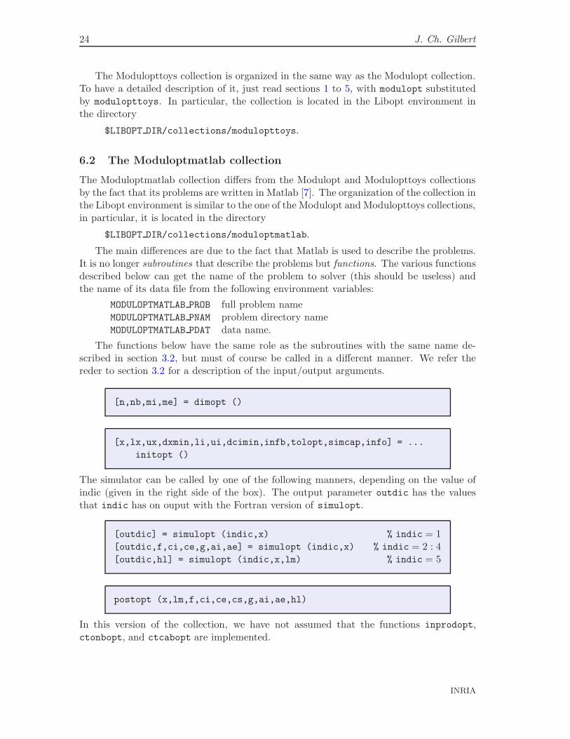
The functions below have the same role as the subroutines with the same name de-scribed in section 3.2, but must of course be called in a different manner. We refer thereder to section 3.2 for a description of the input/output arguments.

[n,nb,mi,me] = dimopt ()

[x,lx,ux,dxmin,li,ui,dcimin,infb,tolopt,simcap,info] = ...

initopt ()

The simulator can be called by one of the following manners, depending on the value ofindic (given in the right side of the box). The output parameter outdic has the valuesthat indic has on ouput with the Fortran version of simulopt.

[outdic] = simulopt (indic,x) % indic = 1[outdic,f,ci,ce,g,ai,ae] = simulopt (indic,x) % indic = 2 : 4[outdic,hl] = simulopt (indic,x,lm) % indic = 5

postopt (x,lm,f,ci,ce,cs,g,ai,ae,hl)

In this version of the collection, we have not assumed that the functions inprodopt,ctonbopt, and ctcabopt are implemented.

INRIA


References

[1] I. Bongartz, A.R. Conn, N.I.M. Gould, Ph.L. Toint (1995). CUTE: Constrained and uncon-strained testing environment. ACM Transactions on Mathematical Software, 21, 123–160. 4

[2] E.D. Dolan, J.J. More, T.S. Munson (2006). Optimality measures for performance profiles.SIAM Journal on Optimization, 16, 891–909. 12

[3] J.Ch. Gilbert, X. Jonsson (2008). LIBOPT – An environment for testing solvers on hetero-geneous collections of problems. Submitted to ACM Transactions on Mathematical Software.3

[4] J.Ch. Gilbert, X. Jonsson (2009). LIBOPT – An environment for testing solvers on hetero-geneous collections of problems – The manual, version 2.1. Technical Report 331 (revised),INRIA, BP 105, 78153 Le Chesnay, France. 3, 6, 19, 21

[5] N. Gould, D. Orban, Ph.L. Toint (2003). CUTEr (and SifDec), a Constrained and Uncon-strained Testing Environment, revisited. ACM Transactions on Mathematical Software, 29,373–394.http://hsl.rl.ac.uk/cuter-www/interfaces.html. 4

[6] C. Lemarechal (1980). Using a Modulopt minimization code. Unpublished Technical Note. 3

[7] Mathworks (2008). The Matlab distributed computing engine.http://www.mathworks.com. 4, 24

Index

basis

canonical, 16orthonormal, 16

cell, 19

collection, 3CUTEr, 4

moduloptmatlab, 3, 24

modulopttoys, 3, 23–24

command (Libopt), see also option, script

addcell, 20

addproblem, 8

rmproblem, 18

comment (in *.lst files), 20

data name, see name/data

directory, 22

bin, 22

collection head, 22interface, 19

libopt head, 5, 22

Modulopt head, 5, 22

problem, 6solver head, 5, 23templates, 8, 23working, 6, 7

environment variableLIBOPT DIR, 5, 22LIBOPT PLAT, 18MODULOPTMATLAB PDAT, 24MODULOPTMATLAB PNAM, 24MODULOPTMATLAB PROB, 24MODULOPT PDAT, 7MODULOPT PNAM, 7MODULOPT PROB, 7WORKING DIR, 7

functionnonsmooth, 12

inner product, 15Euclidean, 15

Kronecker symbol, 16


http://hsl.rl.ac.uk/cuter-www/interfaces.html

http://www.mathworks.com

26 J. Ch. Gilbert

Lagrangian, 4Libopt

environment variable, 5, 22head directory, 5, 22line, 21

libopt run (command), 5–6, 22list

*.lst, 9.collections.lst, 22, 23.solvers.lst, 23all.lst, 5, 6, 8, 19–23comment in a –, 9default.lst, 20links.lst, 9, 18unlinks.lst, 9, 18

Makebin, see script/MakebinMakeclean, see script/MakecleanMakefile

in a problem directory, 8, 17, 18in a solver directory, 7, 10, 22

moduloptmatlab, see collectionmodulopttoys, see collection

namedata – of a problem, pdat, 6– of a problem, prob, 5, 8radical – of a problem, pnam, 6

nondifferentiable, see function/nonsmoothnonsmooth, see function/nonsmooth

optimality conditions, 4option

-c, 18, 20-g, 17-k, 17, 18-p, 18-s, 20-t, 17, 18, 22-v, 8, 17–20, 22-x, 5

pdat, see name/datapnam, see name/radicalprob, see name of a problem

radical name, see name/radical

script, see also command, optionlibopt addcell modulopt, 20libopt addproblem modulopt, 8libopt rmproblem modulopt, 18Makebin, 7–9, 17, 17–18Makeclean, 7, 8, 17, 18solv modulopt, 6–7, 17, 18

solv, 5, 19solv modulopt, see script/solv modulopt

solv modulopt main (main program), 7subroutine

ctcabopt, 16ctonbopt, 16dimopt, 10–11, 21initopt, 11–13, 21inprodopt, 15–16postopt, 14–15, 22simulopt, 13–14, 21

INRIA

Unité de recherche INRIA RocquencourtDomaine de Voluceau - Rocquencourt - BP 105 - 78153 Le ChesnayCedex (France)

Unité de recherche INRIA Futurs : Parc Club Orsay Université- ZAC des Vignes4, rue Jacques Monod - 91893 ORSAY Cedex (France)

Unité de recherche INRIA Lorraine : LORIA, Technopôle de Nancy-Brabois - Campus scientifique615, rue du Jardin Botanique - BP 101 - 54602 Villers-lès-Nancy Cedex (France)

Unité de recherche INRIA Rennes : IRISA, Campus universitaire de Beaulieu - 35042 Rennes Cedex (France)Unité de recherche INRIA Rhône-Alpes : 655, avenue de l’Europe - 38334 Montbonnot Saint-Ismier (France)

Unité de recherche INRIA Sophia Antipolis : 2004, route des Lucioles - BP 93 - 06902 Sophia Antipolis Cedex (France)

ÉditeurINRIA - Domaine de Voluceau - Rocquencourt, BP 105 - 78153 Le Chesnay Cedex (France)

http://www.inria.fr

ISSN 0249-0803

Documents

Organization of the Modulopt collection of optimization