Embed Size (px)
Citation preview

Organ Exchanges:A Fielded Testbed for AI & Healthcare
1
John P. Dickerson Tuomas Sandholm

Tutorial outline
• Introduction & preliminaries• Optimization models & state of the practice• Deep dive into dimensions of kidney exchange:
• Short‐term uncertainty• Fairness vs economic efficiency• Long‐term uncertainty & dynamic optimization• Incorporating human expert judgment in better ways• Incentives & mechanism design
• Other organ exchanges• Conclusion & open research problems
2
Intermission

Tutorial outline
• Introduction & preliminaries• Optimization models & state of the practice• Deep dive into dimensions of kidney exchange:
• Short‐term uncertainty• Fairness vs economic efficiency• Long‐term uncertainty & dynamic optimization• Incorporating human expert judgment in better ways• Incentives & mechanism design
• Other organ exchanges• Conclusion & open research problems
3

4

5

Pair 2
Donor 2
Patient 2
Pair 1
Donor 1
Patient 1
Kidney exchange Idea introduced in 1986 [Rapaport]First exchange (NEPKE) started 2003‐04 [Roth, Sönmez, Ünver, …]
6

Objective: Maximum weight combination of disjoint cycles
7
v1 v2 v3 v4
v5
e1 e3 e5
c1 c2 c3
e8e7
e6e4e2
c4

Cap on cycle length
• Why a cap?• Transplants in a cycle must occur simultaneously• Cycle may fail
• Cap is typically 3
8

Complexity of batch optimization problem
• Theorem [Abraham, Blum, Sandholm EC‐07]
NP‐complete for any cycle length cap ≥ 3
• Solvable in polynomial time if cap=2 or cap=
• See also complexity results by Biró, Manlove, RizziDisc. Math. 09
9
Other barter‐exchange markets
• Holiday Homes: Intervac• Books: Read It Swap It• General used goods: Netcycler / swap.com• National Odd Shoe Exchange• Room exchange (e.g. dorm rooms)• Nurse shift exchange
10

Tutorial outline
• Introduction & preliminaries• Optimization models & state of the practice• Deep dive into dimensions of kidney exchange:
• Short‐term uncertainty• Fairness vs economic efficiency• Long‐term uncertainty & dynamic optimization• Incorporating human expert judgment in better ways• Incentives & mechanism design
• Other organ exchanges• Conclusion & open research problems
11

Pre‐2007 state of the art in kidney exchange clearing algorithms
• Manual matching / greedy algorithms
• (Weighted) maximum matching [Edmonds 1965]
• CPLEX
12

Algorithms for batch problem
• Algorithms find a provably optimal solution• Based on branch‐and‐price framework:
• Branch‐and‐price, DFS pricing [Abraham, Blum, Sandholm EC‐07]
• Branch‐and‐price, B‐F pricing [Glorie et al. MSOM 14, Plaut, Dickerson, Sandholm AAAI‐16]
• Branch‐and‐price, … [Klimentova et al. ICCSA‐14, Manlove & O’Malley ACM JEA 14, Mak‐Hau J. Comb Opt 15, ...]
• Based on constraint generation:• Basic, not scalable [Abraham, Blum, Sandholm EC‐07]
• Based on PC‐TSP [Anderson et al. PNAS 2015]• Compact formulations:
• Extended edge formulation [Constantino et al. EJOR 2014]• Position‐indexed [ongoing work with CMU and Manlove & Trimble at U. Glasgow]
13

Kidney exchanges use designs, algorithms, and software from Prof. Sandholm’s lab
• United Network for Organ Sharing (UNOS)• Our technology was selected • Exchange went live Oct. 2010• Match run twice a week• 143 transplant centers
• Previously:• Alliance for Paired Donation• Paired Donation Network
14

UNOS has design constraints that private exchange don’t have
• Must have transparent, broadly‐agreed policies• Clearing algorithm / priority points must be transparent
• AI must be autonomous (surgeons still have veto)• Have to work also with small transplant centers => slower turnaround time
• …
15
A first approach: Constraint (row) generation[Abraham, Blum, Sandholm, EC‐07]
16

Special Case: No limit on cycle length
• Polynomial‐time solvable via max‐weight perfect matching
• Red vertex for each patient, blue vertex for each donor
• Edge between each patient and their incompatible donor with weight 0
(=> perfect matching)
• Edge between patient and compatible donor with weight 1
• Exchanges correspond to perfect matchings
17
v1 v2 v3 v4
v5
e1 e3 e5
c1 c2 c3
e8e7
e6e4e2
c4
Items
Agentsv1 v2 v3 v4 v5
e1 e3 e8
e2
v1 v2 v3 v4 v5
e7e6
e5
e4

ILP: Edge Formulation (in original directed graph)
• Max ∑e w(e)*e• Subject to:
• Conserva on: ∑eOut(vi)e ‐ ∑eIn(vi)e = 0• Capacity: ∑eOut(vi) e ≤ 1 for all vi• e {0,1} for each edge e
• Limit L on cycle length:• For each (non‐cycle) path p of length L:
∑ep e ≤ L ‐ 1
18
v1 v2 v3 v4
v5
e1 e3 e5
c1 c2 c3
e8e7
e6e4e2
c4

Constraint (= Row) Generation
• ILP too large (too many constraints)• Even with only 1000 patients, there are 400M length‐3 paths
• Incremental formulation• Begin with small subset of constraints• Repeat
• Solve LP relaxation• Add subset of violated constraints, if any
• Perform Branch‐and‐Bound, doing the repeat loop above at every node
19

Constraint Generation …• Constraint Seeding:
• Forbid any (non‐cycle) path of length L‐1 that has no edge closing the cycle from its tail to head
• Or, seed with random constraints from the ILP
• Constraint Generation:• Find length‐L path with value sum more than L – 1
• A long cycle C contains |C| of these paths• Or, more space efficient to add only one constraint for such a cycle: Edge sum in
a long fractional cycle can be at most floor( ([L‐1]/L)*|C| ) => slower• So we went in the other direction: Add a constraint per violating path p, and
each path with the same interior vertices => faster
20

A First Approach: Constraint (Row) Generation in Edge Formulation
• Even after many improvements, could not clear markets with 100 nodes faster than our second approach with 10,000 nodes
• Theorem. LP relaxation of edge formulation not as tight as that of cycle formulation
21

A better algorithm (early version of what we fielded at UNOS)[Abraham, Blum, Sandholm, EC‐07]
22

Special Case: Cycle Length L ≤ 2
• Model using a different graph:• One undirected edge for each cycle of length at most 2
• Edge weight is weight of cycle• Exchanges correspond to matchings• Polytime to find max‐weight matching in general graph
23
v1 v2 v3 v4
v5
e1 e3 e5
c1 c2 c3
e8e7
e6e4e2
c4
c_1
v_1 v_2 v_3 v_4
c_3c_2

ILP: Cycle formulation
• C(L) ≡ set of cycles of length ≤ L• One variable for each cycle c in C(L)• Max ∑c C(L) wc xc• Subject to:
• ∑ c : vi c xc ≤ 1 (each vi belongs to at most one cycle)
• xc {0,1} for all c C(L)
24

Solving the ILP• Too large to write down
• Unlike winner determination in combinatorial auctions
• Overall approach: Branch‐and‐Price• Branch: select fractional column and fix its value to 1 and 0 respectively
• Fathom the search node if no better than incumbent• Solve LP relaxation using column generation
26
x7
x4
1 0
1 0
… …
…

Column generation• Master LP P has too many variables
• Won’t fit in memory• Would take too long to solve
• Begin with restricted LP P’, which contains only a small subset of the variables (i.e., cycles)
• OPT(P’) ≤ OPT(P)• Solve P’ and, if necessary, add more variables to it
• Repeat until OPT(P’) = OPT(P)
28

“Pricing” problem
• Price of a cycle (i.e., column) c is • p(c) = wc ‐ ∑v in c dual‐val(v)
• Dual constraint c is violated if p(c) > 0• Pricing problem: find a positive price cycle, or report that none exists (in which case OPT(P’) = OPT(P))
• Key: Check the price of cycles one‐by‐one, without having all cycles in memory
32

Pricing problem: Further techniques to enhance speed• Generate cycles by DFS over input graph
• Vertices explored in non‐decreasing order of dual value• Earlier vertices more likely to belong to positive‐price cycle• Can prune DFS path early
• Avoid repeating parent’s pricing problem work in child’s pricing problem
• If a vertex wasn’t the root of any positive price cycle, and its dual value hasn’t decreased, then it can’t be the root of a positive‐price cycle now either
33

“Tailing off” effect
• OPT(P’) = OPT(P), but some columns still have positive price
• Many iterations required to prove optimality
• Our technique for tackling this led to big speedup• Polytime upper bound by removing cycle length constraint
• Edge formulation in bipartite perfect‐matching graph (integrality gap 0, so we can just solve that LP instead of that ILP)
• Column (edge here) generation• Fastest polynomial‐time maximum‐weight matching code didn’t scale
[Rothberg DIMACS implementation challenge 1990]
• Optimal once incumbent value = upper bound• Length‐3 cycles usually enough to match upper bound
34

Column seeding
• Pricing problem is expensive & improving OPT(P’) is slow
• => Want to begin with OPT(P’) close to OPT(P)• => Select good (but small) set of initial columns
• Begin with columns from heuristic solutions• E.g. randomized greedy and max‐weight matching• Perform well and introduce very few columns
• Also, random selection of larger set of cycles (400,000)
35

Column management
• Problems with too many columns in P’• Run out of memory, even with ≤ 4000 vertices• LPs take longer to solve
• Delete columns so P’ is not too big• Only a small fraction of columns end up in the final solution for OPT(P) => unlikely to delete
• Will always generate again if needed• Delete column with largest negative price first, as this is the most satisfied constraint in D
• But some columns we never delete, e.g., those we have branched on and those with positive LP value
36

Primal heuristics1. Rounding heuristic: include all cycles with LP value at least ½ ;
greedily select remaining cycles• Rarely helps
2. Our heuristic:• P’ at root node usually contains enough columns so that
integral OPT can match fractional OPT• We use CPLEX MIP as a primal heuristic at nodes, but only on
the restricted ILP that corresponds to P’• Constraint that ILP value has to match fractional target, and• Time limit, and• Only do this if node has sufficiently different set of cycles than its parent
• Improves speed significantly
37

Experiment using data generator by [Saidman et al. 06]Cycle cap = 3
40Predicted size of US‐wide kidney exchange
CPLEX (cycle formulation)
Our algorithm
Our algorithmwith no randomcolumns
Our algorithmwith no optimality prover

Recap: Main message
• This algorithm made modern kidney exchanges able to be cleared in a scalable way
• Techniques that made this possible• Incremental problem formulation• Exploiting problem specific upper bounds in several ways• Other algorithmic ideas
41

Additional functionality for modern kidney exchanges supported by this algorithm and its later enhancements
43

Side constraints
• Algorithm supports certain kinds of side constraints, e.g.,• Center A does not want to be in cycles longer than 2• Patient x does not want to be in a cycle longer than 2• Center B does not want to participate in altruistic donor chains of length greater than 3
• …
44

Multiple willing donors per patient
• All their edges included in input graph• Solver automatically uses at most one of the donors
45

Incorporating compatible pairs
• Why?• Patient can get a better kidney• Others get more/better matches
• Our algorithm supports this• Could preprocess so patient can’t get worse kidney than her compatible donor brings
46

Incorporating list exchange(s)
• Algorithm can be used also if list exchanges were included in the optimization
47

Weights on edges
• Algorithm supports weights on edges (thus also on nodes)
• Weights can represent, e.g.,• Degrees of compatibility• Projected life years (potentially quality‐adjusted)• Travel distance• Wait time• Transplanting children• Transplanting sensitized, hard‐to‐match patients
• Tradeoffs between efficiency and fairness• AI autonomy
48
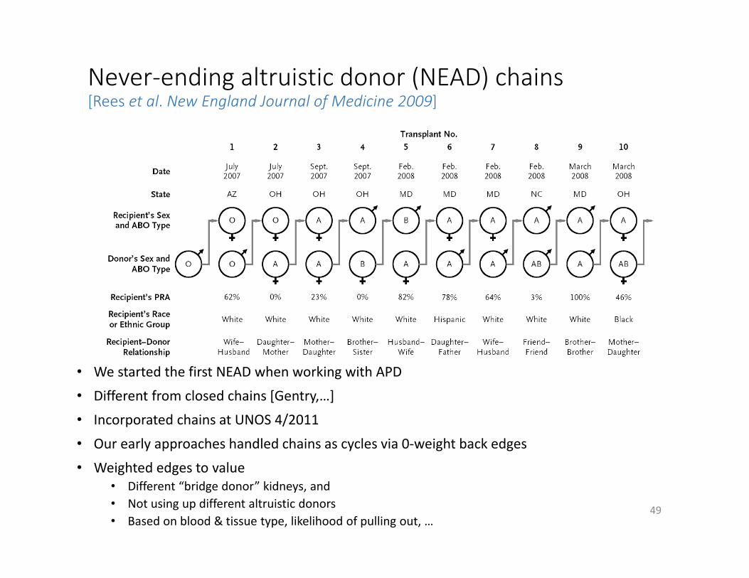
Never‐ending altruistic donor (NEAD) chains[Rees et al. New England Journal of Medicine 2009]
• We started the first NEAD when working with APD
• Different from closed chains [Gentry,…]
• Incorporated chains at UNOS 4/2011
• Our early approaches handled chains as cycles via 0‐weight back edges
• Weighted edges to value• Different “bridge donor” kidneys, and• Not using up different altruistic donors• Based on blood & tissue type, likelihood of pulling out, …
49

50
[National Kidney Registry]
30‐chain [New York Times 2/18/2012]
Study of chains[Dickerson, Procaccia & Sandholm, AAMAS‐12]
51
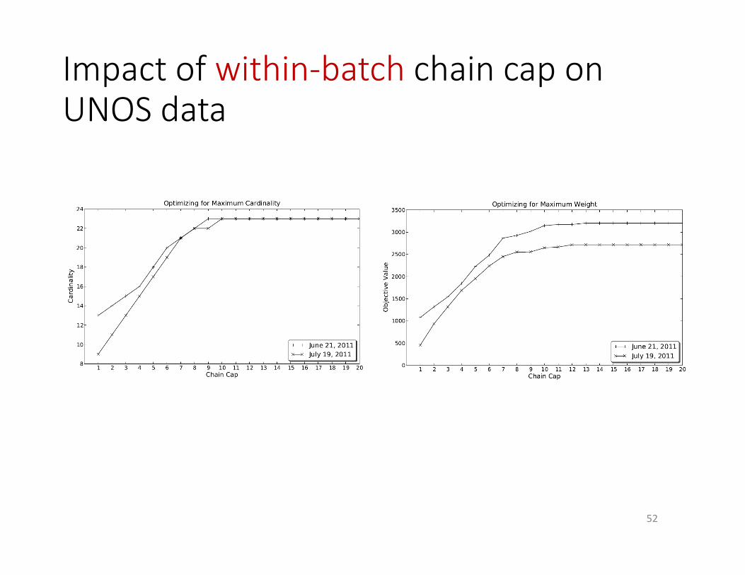
Impact of within‐batch chain cap on UNOS data
52

Theory: Short chains suffice• ABO‐model with tissue type incompatibility• Large, unweighted graph
53

Why the discrepancy?• Possible reasons:
• Unweighted – not the (only) reason• UNOS data not “large”• Uniform tissue type incompatibility model not realistic
• Experiments using Saidman et al. generator:
• In dynamic experiments, a chain cap of 4 was best
54
Newer scalable clearing algorithms
55

• Builds on the prize‐collecting traveling salesperson problem[Balas Networks 1989]
• PC‐TSP: visit each city (patient‐donor pair) exactly once, but with the additional option to pay some penalty to skip a city (penalized for leaving pairs unmatched)
• They maintain decision variables for all cycles of length at most L, but build chains in the final solution from decision variables associated with individual edges
• Then, an exponential number of constraints could be required to prevent the solver from including chains of length greater than K; these are generated incrementally until optimality is proved.
• Leverage cut generation from PC‐TSP literature to provide stronger (i.e. tighter) IP formulation
56
Better batch algorithms, infinite chain caps[Anderson et al. PNAS 2015]

• Idea: solve a structured alternate optimization problem that implicitly prices variables
• Price (for max card, weight): wc – Σv in c δv• But: wc= Σe in c we
• Take G=(V,E), create G’=(V,E) s.t. all edges e = (u,v) are reweighted re = δv – we
• Positive price cycles in G = negative weight cycles in G’• Bellman‐Ford finds shortest paths
• Undefined in graphs with negative weight• Shortest path is NP‐hard (reduce from Hamiltonian path:
• Set edge weights to ‐1, given edge (u,v) in E, ask if shortest path from u to v is weight 1‐|V| visits each vertex exactly once
• We only need some short path (or proof that no negative cycle exists)• Now pricing runs in time O(|V||E|cap), but …
57
Better batch algorithms under within‐batch chain caps[Glorie et al. MS&OM 2014]
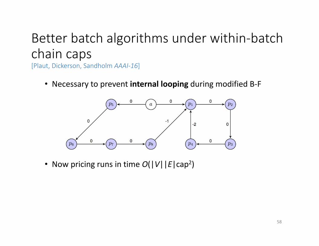
• Necessary to prevent internal looping during modified B‐F
• Now pricing runs in time O(|V||E|cap2)
58
Better batch algorithms under within‐batch chain caps[Plaut, Dickerson, Sandholm AAAI‐16]

Experiment with 300 vertices, 1 hour time limiton realistic generated UNOS graphs
59
3 altruists 6 altruists 15 altruists 75 altruists
Better batch algorithms under within‐batch chain caps[Plaut, Dickerson, Sandholm AAAI‐16]

• Previous models: exponential #constraints (CG methods) or #variables (B&P methods)
• Let L be upper bound on #cycles in a final matching
• Create L copies of compatibility graph
• Search for a single cycle or chain in each copy• (Keep cycles/chains disjoint across graphs)
60
Compact formulations[Constantino et al. EJOR 2014]

7a: max edge weights over all graph copies7b: give a kidney <‐> get a kidney within that copy7c: only use a vertex once7d: cycle cap
Compact formulations[Constantino et al. EJOR 2014]
Poly #constraints and #variables!

• Previous: edge is in a cycle/chain or not• Weak LP relaxation
• Idea: where in the cycle/chain does the edge exist?• “Position indexed”
62
Compact formulations for within‐batch chain caps[ongoing with David Manlove & James Trimble]

3a: max weight of edges in chains + weight of cycles3b: each pair is in at most chain/cycle3c: each NDD has at most one used out edge3d: if an edge is used at position k+1 in chain, there must be an appropriate edge used at position k in that chain
Compact formulations for within‐batch chain caps [ongoing with David Manlove & James Trimble]

How to choose a formulation
• Comparison of LP relaxations• Column‐generation‐based tend to have tighter relaxations (so far!)
• Business constraints• Constraint‐generation‐based approaches outperform when feasible matching space is less constrained
• E.g., no chain cap …• Column‐generation‐based approaches allow for more expressive objective functions (so far!)
• E.g., general stochastic matching

Fielded kidney exchanges• NEPKE (started 2003‐04, now closed)• United Network for Organ Sharing (UNOS)• Alliance for Paired Donation• Paired Donation Network (now closed)• National Kidney Registry• San Antonio• Mayo Clinic• St. Barnabas Compassionate Share• Canada• Netherlands• UK• Australia• Portugal • Israel (about to start)• Sweden (about to start Q1 2016)
65
~600transplants in US per year, mainly via open chains
Only US one that uses purely algorithmic matching

State of practice• United States:
• Started in the US in 2003‐04 (NEPKE; pool now merged to UNOS pool), cycles
• UNOS nationwide exchange (only one that is run by algorithms)• Several private exchanges (NKR, APD) and single‐center “exchanges”
• ~600 transplants per year, mostly via open chains• Multi‐listing, competition, sniping• Cadence: twice a week or even multiple times per day
• Netherlands: national, chains, algorithms• UK: national, quarterly, hierarchical algorithmic approach• Canada: national, quarterly, CPLEX• Nascent: Australia, Portugal, Israel, Sweden, …• International: one swap at APD so far via manual matching
66
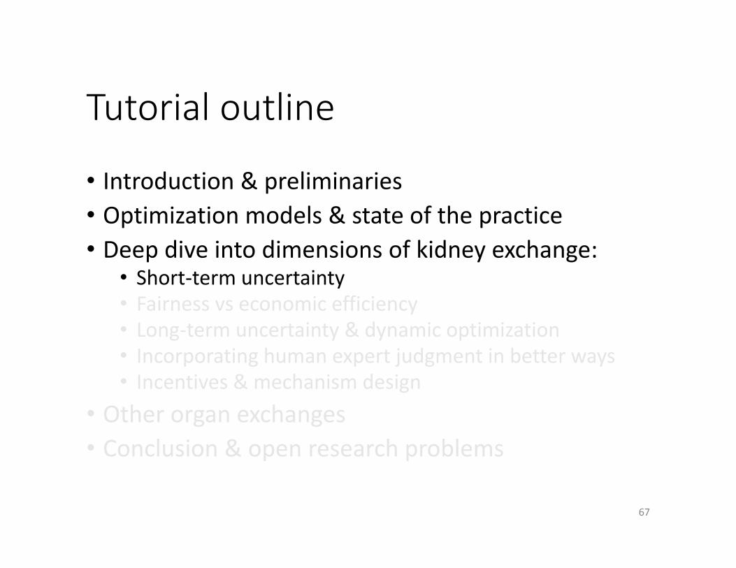
Tutorial outline
• Introduction & preliminaries• Optimization models & state of the practice• Deep dive into dimensions of kidney exchange:
• Short‐term uncertainty• Fairness vs economic efficiency• Long‐term uncertainty & dynamic optimization• Incorporating human expert judgment in better ways• Incentives & mechanism design
• Other organ exchanges• Conclusion & open research problems
67

Matched ≠ Transplanted
• Only around 8% of UNOS matches resulted in an actual transplant
• Similarly low % in other exchanges [ATC 2013]
• Many reasons for this. How to handle?
• One way: maximize expected value of the (batch) transplants
68

Failure‐aware model [Dickerson Procaccia Sandholm EC‐13]
• Compatibility graph G• Edge (vi, vj) if vi’s donor can donate to vj’s patient • Weight we on each edge e
• Success probability qe for each edge e
• Discounted utility of cycle cu(c) = ∑we ∏qe
69
Value of successful cycle Probability of success

Failure‐aware model…• Discounted utility of an (unweighted for simplicity) k‐chain c
• These cycle and chain utilities are not the same one would get by simply replacing the weight of each edge by (weight * success probability)
• Utility of a solution M: u(M) = ∑ u(c)
70
Exactly first i transplants execute Chain executes in entirety

Our problem
• Discounted clearing problem is to find matching M*
with highest discounted utility
71
1 2
3
Maximum cardinality Maximum expected transplants
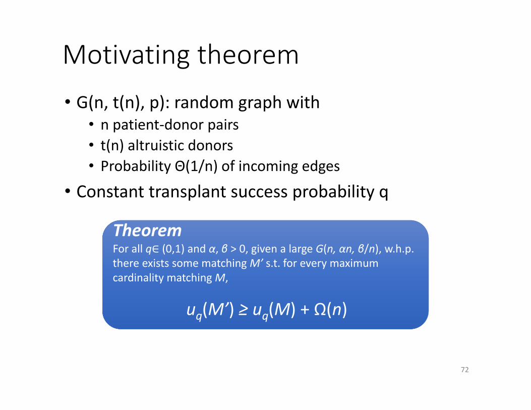
Motivating theorem• G(n, t(n), p): random graph with
• n patient‐donor pairs• t(n) altruistic donors• Probability Θ(1/n) of incoming edges
• Constant transplant success probability q
72
TheoremFor all q∈ (0,1) and α, β > 0, given a large G(n, αn, β/n), w.h.p. there exists some matching M’ s.t. for every maximum cardinality matching M,
uq(M’) ≥ uq(M) + Ω(n)

Proof sketch: Counting Y‐gadgets
• For every structure X of constant size, w.h.p. can find Ω(n) structures isomorphic to X and isolated from the rest of the graph
• Label them (alt vs. pair): flip weighted coins, constant fraction are labeled correctly constant × Ω(n) = Ω(n)• Direct the edges: flip 50/50 coins, constant fraction are entirely directed correctly constant × Ω(n) = Ω(n)
73

In theory, we’re losing out on expected actual transplants by maximizing match cardinality.
… What about in practice?
74

UNOS2010‐2014
75

Solving this new problem
• Real‐world kidney exchanges are still small• UNOS pool: 281 donors, 260 patients [2 Feb 2015]
• Undiscounted clearing problem is NP‐hard when cycle/chain cap L ≥ 3 [Abraham et al. 2007]
• Special case of our problem
• Current UNOS solver will not scale to this problem• Empirical intractability driven by chains
76

Algorithm changes for this probabilistic setting• Use chain extension in pricing problem
• Theorem. Don’t have to extend a chain by any finite #steps if optimistic infinite extension has negative expected value:
• Ordering heuristics for cycle and chain generation
• Upper bound now hard• Theorem. Discounted clearing NP‐complete (even with no chains or cycle length cap)• So, we use looser bound: solve with w’e = (1‐pfail) we
• Lower bound still easy• Theorem. Discounted clearing with 2‐cycles polytime
Donation to waitlist
Discounted utility of current chain
Optimistic future value of infinite extension
Pessimistic sum of LP dual values

Scaling experiments
80
|V| CPLEX Ours Ours without chain curtailing
10 127 / 128 128 / 128 128 / 128
25 125 / 128 128 / 128 128 / 128
50 105 / 128 128 / 128 125 / 128
75 91 / 128 126 / 128 123 / 128
100 1 / 128 121 / 128 121 / 128
150 114 / 128 95 / 128
200 113 / 128 76 / 128
250 94 / 128 48 / 128
500 107 / 128 1 / 128
700 115 / 128
900 38 / 128
1000
• Runtime limited to 60 minutes; each instance given 8GB of RAM.• |V| represents #patient‐donor pairs; additionally, 0.1|V| altruistic donors are present.

Dynamic experiment with failures 24 weeks; Bimodal failure probability; #altruists = 0.1 * #pairs
81

Pre‐match edge testing[Blum et al. EC‐13 and EC‐15]
• Complementary idea: perform a small amount of testing before a match run to query for (non)existence of edges
• more extensive medical testing• donor interviews• surgeon interviews, etc.
• For 2‐cycles only: stochastic matching
83

The power of two crossmatches[Blum et al. EC‐13]
• Cast as a general stochastic matching problem:
• Initially: 2‐cycles only (= undirected), at most 2tests per vertex polytime algorithm for this
Given a graph G(V,E), choose subset of edges S such that:
|M(S)| ≥ (1‐ε) |M(E)|
Need: “sparse” S, where every vertex has O(1) incident tested edges

Pre‐match testing in rounds[Blum et al. EC‐15]
• What about testing a variable number of edges per vertex?
• What if we can test edges, get feedback, test more?• What about 3‐cycles, chains?• Cast as an adaptive stochastic k‐set packing problem:
• Query edges in rounds, where each round tests at most one incident edge per vertex

General theoretical results[Blum et al. EC‐15]
Stochastic matching: (1‐ε) approximation with Oε(1) queries per vertex, in Oε(1) rounds
Stochastic k‐set packing: (2/k – ε) approximation with Oε(1) queries per vertex, in Oε(1) rounds
Adaptive: select one edge per vertex per round, test, repeat
Non‐adaptive: select O(1) edges per vertex, test all at once
Stochastic matching: (0.5‐ε) approximation with Oε(1) queries per vertex, in 1 round
Stochastic k‐set packing: (2/k – ε)2 approximation with Oε(1) queries per vertex, in 1 round

Adaptive algorithm
87
r Base graph Matching picked Result of queries
1:
2:
Input Graph
For R rounds, do:1. Pick a max‐cardinality matching M in graph G,
minus already‐queried edges that do not exist2. Query all edges in M

Intuition for adaptive algorithm
• If at any round r, the best solution on edges queried so far is small relative to omniscient …
• ... then current structrure admits large number of unqueried, disjoint augmenting structures
• For k=2, simply augmenting paths• Augmenting structures might not exist, but can query in parallel in a single round
• Structures are constant size exist with constant probability
• Structures are disjoint queries are independent• Close a constant gap per round
88

UNOS Data
89
Even 1 or 2 extra tests would result in a huge lift
At p=0.5, one edge test per vertex +21% OPT
Tutorial outline
• Introduction & preliminaries• Optimization models & state of the practice• Deep dive into dimensions of kidney exchange:
• Short‐term uncertainty• Fairness vs economic efficiency• Long‐term uncertainty & dynamic optimization• Incorporating human expert judgment in better ways• Incentives & mechanism design
• Other organ exchanges• Conclusion & open research problems
90

An initial definition of fairness[Roth, Sönmez, Ünver JET 2006]
• Matching lottery: distribution over possible matchings
• Example lottery:
• Utility profile: total probability given to each vertex
Example due to[Li et al. AAMAS‐14]
u v w z
:
::::
u v w zu v
v ww zℓ ℓ 0.5
ℓ ℓ ℓ 0
ℓ, ℓ, ℓ , ℓ 0.5,1.0,1.0,0.5

• One utility profile x is said to Lorenz dominate another utility profile y if:
• Sort both profiles in increasing order• Condition 1: For t = {1..n}, ∑ ∑• Condition 2: There exists t s.t. ∑ ∑
• Previous graph: Lorenz dominant profile assigns all weight to
• Algorithm is exponential in graph size (#odd components in Gallai‐Edmonds Decomposition)
• Applies to 2‐cycles only
An initial definition of fairness[Roth, Sönmez, Ünver JET 2006]
Thm: There is a unique Lorenz‐dominant utility profile.
: u v w z
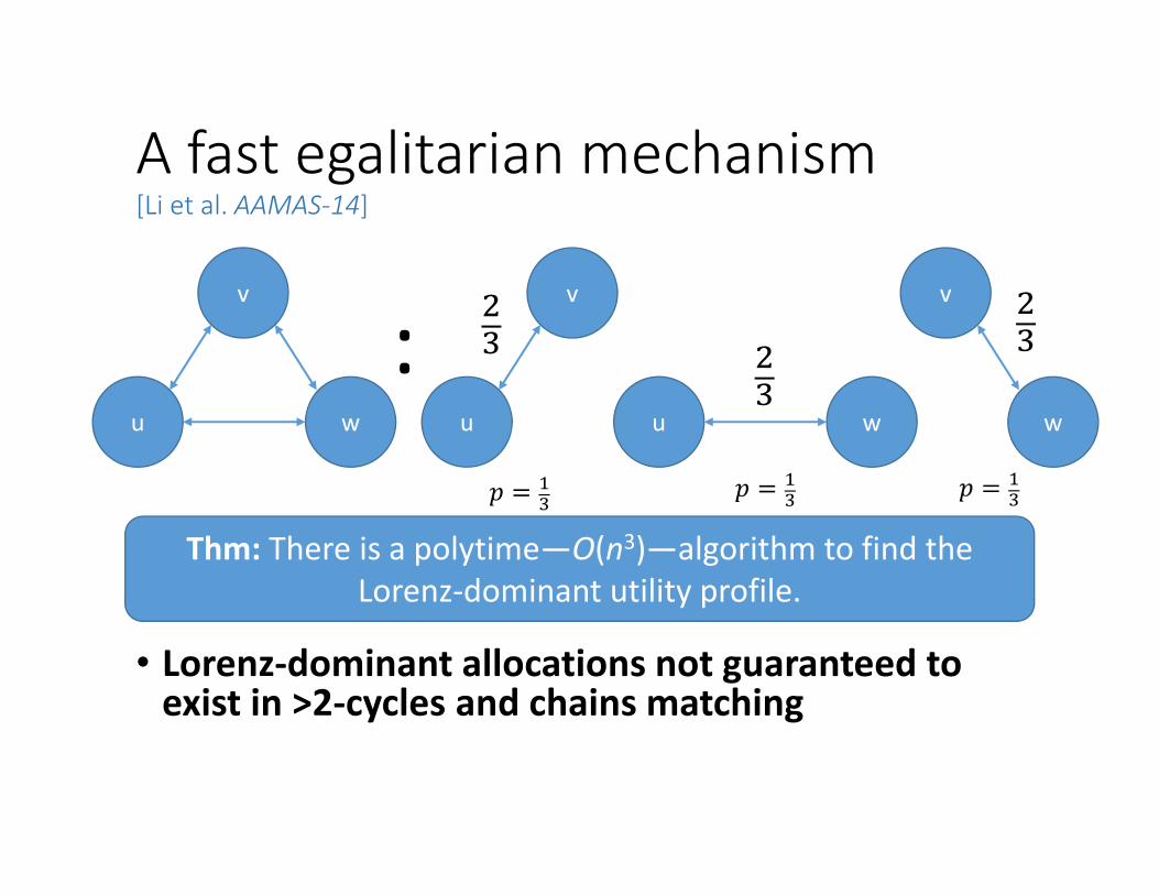
A fast egalitarian mechanism[Li et al. AAMAS‐14]
• Lorenz‐dominant allocations not guaranteed to exist in >2‐cycles and chains matching
Thm: There is a polytime—O(n3)—algorithm to find the Lorenz‐dominant utility profile.
u
v
w
:u
v
u w
v
w

Balancing efficiency and equity
• Fielded kidney exchanges match under utilitarian or near‐utilitarian rules:
• i.e., “match as many as possible”• (often with some ad‐hoc vertex weighting)
• This can marginalize hard‐to‐match pairs
94
Present‐day marginalization
• Highly‐sensitized patients have elevated antibody levels that negatively react to foreign tissue
• Harder to find a matching donor
• CPRA score estimates % of incompatible donors• 0%: low sensitization, easy to find a match• 100%: high sensitization, hard to find a match• Typical definition of highly sensitized is 80% (and increasing); 80% is what we will use below
• 17% of adult deceased‐donor kidney waitlist is highly‐sensitized
• ~60% in kidney exchange
95

96

“The needs of the many outweigh the needs of the few or the one.”
• … Generally not followed in healthcare
97
DefinitionPrice of fairness: relative loss in system efficiency due to using a fair objective [Bertismas, Farias, Trichakis OR 2011, Caragiannis et al. WINE‐09]
98

“Price of fairness” in kidney exchange[Dickerson, Procaccia, Sandholm AAMAS‐14, invited AIJ]
99
• Price of fairness: relative loss of match efficiency due to fair utility function
• Clearing problem: find a matching M* that maximizes utility function
∗ argmax∈
,∗ ∗
∗
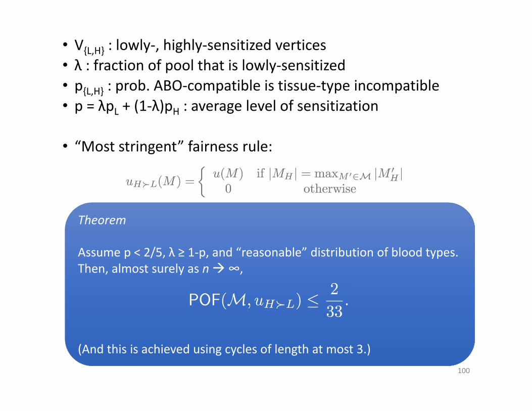
• V{L,H} : lowly‐, highly‐sensitized vertices• λ : fraction of pool that is lowly‐sensitized• p{L,H} : prob. ABO‐compatible is tissue‐type incompatible• p = λpL + (1‐λ)pH : average level of sensitization
• “Most stringent” fairness rule:
100
Theorem
Assume p < 2/5, λ ≥ 1‐p, and “reasonable” distribution of blood types.Then, almost surely as n∞,
(And this is achieved using cycles of length at most 3.)

In theory, the price of fairness is low
101
As many highly‐sensitized patients as possible are matched; loss compared to the efficient matching of [Ashlagi & Roth EC‐11] is shown with wavy lines.

From theory to practice
• Theoretical assumptions (standard):• Big graphs (“n∞”)• Dense graphs (constant p, pL, pH)• Cycles (no chains)• No post‐match failures• Simplified patient‐donor features
• Fairness criterion was extremely strict• In healthcare, important to work within (or near to) the constraints of the fielded system
• [Bertsimas, Farias, Trichakis 2013]• Our experience with UNOS
102

Two fairness definitions
• Lexicographic:• Generalizes strict uH>L used in theoretical result
• Requires fraction α of the maximum number of highly‐sensitized patients that could be matched over all possible matchings
• Chooses the largest matching among those
• Weighted:• A highly‐sensitized patient counts for (1+β) times as much as a lowly‐sensitized patient
103

Implementing the two fairness notions within branch‐and‐price
• Lexicographic: difficult• Requires a matching‐wide constraint• Finding a positive price cycle now requires solving an integer program (at every node in search tree)
• In experiments we used CPLEX
• Weighted: easy• Re‐weight edges according to fairness function• Match using our solver
104

Fairness experiments on UNOS data
• Our algorithm and code run the UNOS nationwide exchange
• Algorithm computes a weighted efficient matching
• Applied both fairness definitions to 73 match runs, compared against fielded version
• (All match runs from inception of exchange in Oct. 2010 through early Oct 2013)
108

Strict lexicographic fairness on UNOS data
109

Weighted fairness on real UNOS data
110

Experiments on generated data
• Two standard kidney exchange models:• [Saidman et al. 2006]: dense, parameterized by full US population, considers ABO and 3 levels of sensitization, etc.
• [Ashlagi et al. EC‐12+]: adaptation of sparse Erdos‐Renyigraphs:
• no blood type• high and low sensitization
• constant prob of incoming edge to low‐sensitized patients• Θ(1/n) prob to high‐sensitized patients
• Created a third distribution, “Saidman‐UNOS”:• Saidman model parameterized by UNOS pool data (Oct 2013)
111

Avg (St.Dev.) efficiency loss under the strict fairness, for generated data
Size Saidman (US) Saidman (UNOS) Ashlagi & Roth10 0.24% (1.98%) 0.00% (0.00%) 0.98% (5.27%)25 0.58% (1.90%) 0.19% (1.75%) 0.00% (0.00%)50 1.18% (2.34%) 1.96% (6.69%) 0.00% (0.00%)
100 1.46% (1.80%) 1.66% (3.64%) 0.00% (0.00%)150 1.20% (1.86%) 2.04% (2.51%) 0.00% (0.00%)200 1.43% (2.08%) 1.55% (1.79%) 0.00% (0.00%)250 0.80% (1.24%) 1.86% (1.63%) 0.00% (0.00%)500 0.72% (0.74%) 1.67% (0.82%) 0.00% (0.00%)
112
• Distributions align more with our theoretical model (of a larger, stable exchange) than UNOS data does– Thus the price of fairness is much lower

Experiments on the interaction between failure‐aware matching and fairness rules
113
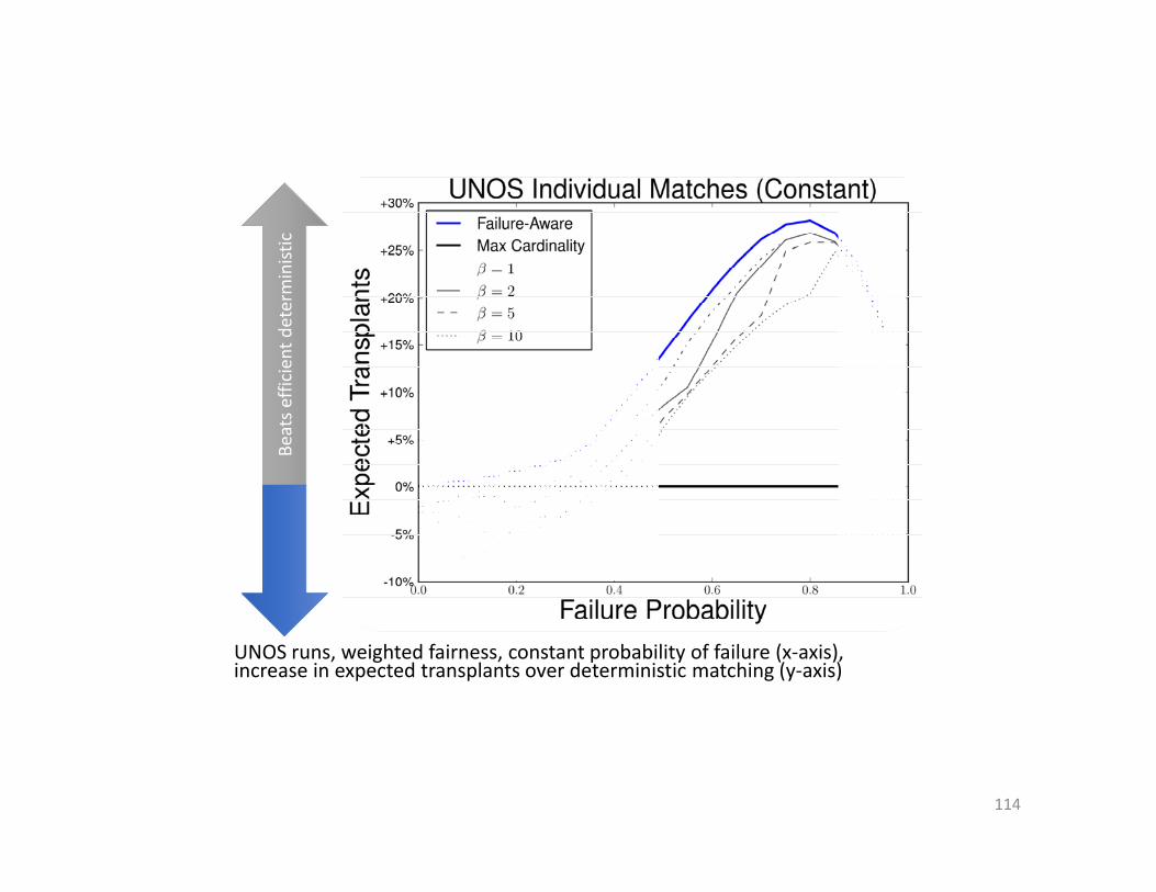
UNOS runs, weighted fairness, constant probability of failure (x‐axis), increase in expected transplants over deterministic matching (y‐axis)
114
Beats e
fficient d
eterministic

Generated UNOS runs, weighted fairness, constant probability of failure (x‐axis), increase in expected transplants over deterministic matching (y‐axis)
115

Generated (top row) and real (bottom row) UNOS runs, weighted fairness (x‐axis), bimodal failure probability (APD failures in left column, UNOS failures in right column), increase in expected transplants over deterministic matching (y‐axis)
116

Take‐home message
• In theory, the price of fairness is small
• In practice, the situation is trickier – but someemphasis on fairness can be added without much drop in overall efficiency
• Present‐day kidney exchange models and solvers are amenable to fairness criteria
117

Tutorial outline
• Introduction & preliminaries• Optimization models & state of the practice• Deep dive into dimensions of kidney exchange:
• Short‐term uncertainty• Fairness vs economic efficiency• Long‐term uncertainty & dynamic optimization• Incorporating human expert judgment in better ways• Incentives & mechanism design
• Other organ exchanges• Conclusion & open research problems
118

Dynamic kidney exchange
• Kidney exchange is naturally dynamic• Can be described by the evolution of its graph:
• Additions, removals of edges and vertices
119
Vertex Removal Edge Removal Vertex/Edge AddTransplant, this exchange Matched, positive crossmatch Normal entranceTransplant, deceased donor waitlist Matched, candidate refuses donor Transplant, other exchange ("sniped") Matched, donor refuses candidateDeath or illness Pregnancy, sickness changes HLA Altruist runs out of patience Bridge donor reneges
Initial theoretical work• Ünver [RES 2010] studies minimizing avg wait time in kidney exchange
• 2‐cycles or no cycle cap; no chains• No tissue type incompatibility• No pairs expire• Poisson arrivals• Proves that simple dispatch rules are optimal
• Zenios [Mgmt Sci 2002] studies maximizing avg quality‐adjusted life years
• 2‐cycles only (no longer cycles, no chains) • Only two types of patient‐donor pairs• Models exchange as a divisible birth and death process• No matching aspects of the problem• No patients expire, but long wait penalized by a fixed cost• Optimal policy is analytically derived
• Limits the number of patients that can take part in exchange. Patients not admitted queue for altruistic donors (wait time here assumed zero)
121

No good prior‐free online algorithm (even without chains)• Proposition. No deterministic prior‐free algorithm can achieve competitive ratio better than L/2
• Proposition. No prior‐free algorithm can achieve competitive ratio better than 2 – (2/L)
• => Have the algorithm use distributional information• But full stochastic optimization totally unscalable here
122
[Awasthi and Sandholm IJCAI‐09]
Family 1 of approaches [Awasthi and Sandholm IJCAI‐09]
• At each step• Draw sample trajectories• Leverage our offline algorithm to pick an action, i.e., combination of cycles and chains (not policy)
123
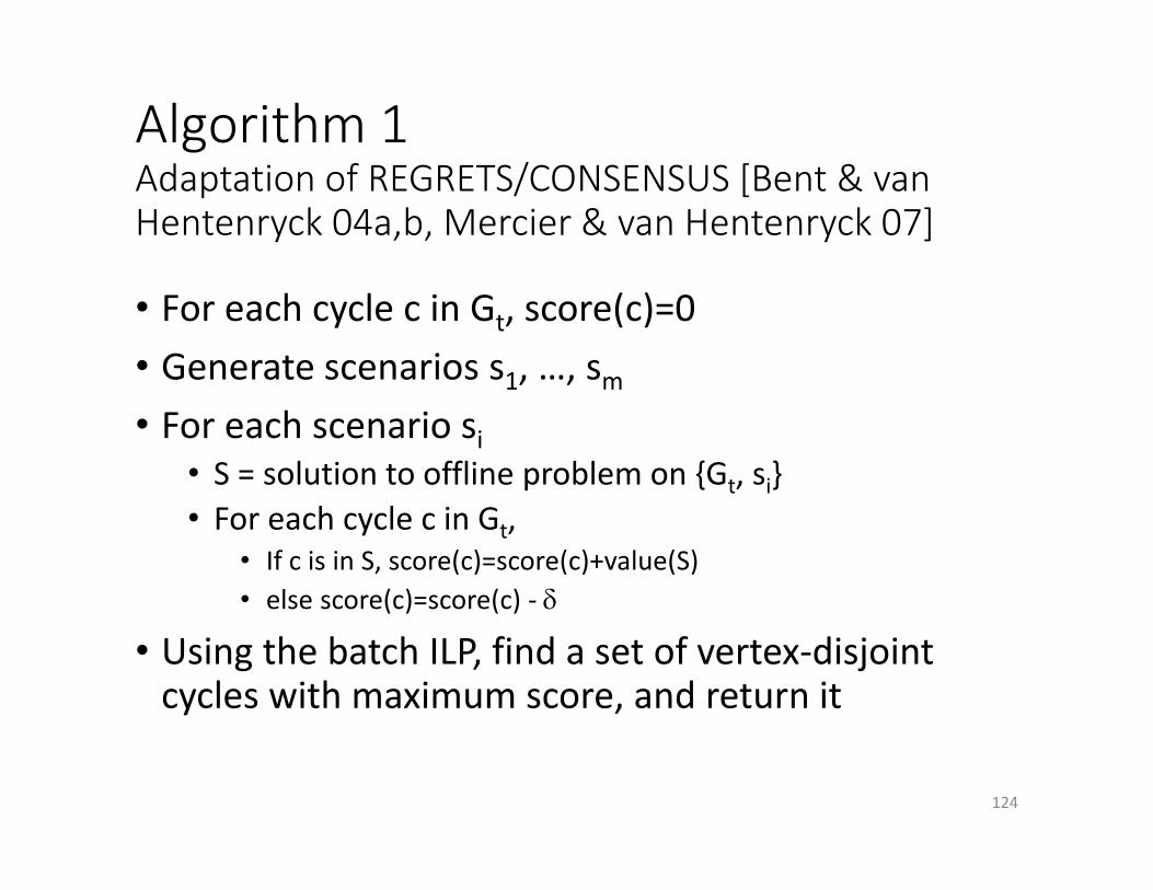
Algorithm 1Adaptation of REGRETS/CONSENSUS [Bent & van Hentenryck 04a,b, Mercier & van Hentenryck 07]
• For each cycle c in Gt, score(c)=0• Generate scenarios s1, …, sm• For each scenario si
• S = solution to offline problem on {Gt, si}• For each cycle c in Gt,
• If c is in S, score(c)=score(c)+value(S)• else score(c)=score(c) ‐
• Using the batch ILP, find a set of vertex‐disjoint cycles with maximum score, and return it
124

Interior value of δ was best
126

Algorithm 1 is not optimal
127
ABCD exist. In step 2, A disappears, and either EF or GH appear.
Optimal solution is cycle ACDB, but that is not optimal on any trajectory!
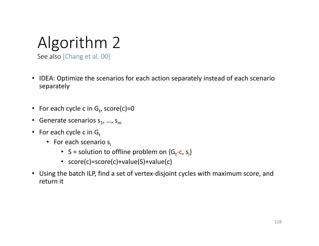
Algorithm 2See also [Chang et al. 00]
• IDEA: Optimize the scenarios for each action separately instead of each scenario separately
• For each cycle c in Gt, score(c)=0
• Generate scenarios s1, …, sm• For each cycle c in Gt
• For each scenario si• S = solution to offline problem on {Gt‐c, si}• score(c)=score(c)+value(S)+value(c)
• Using the batch ILP, find a set of vertex‐disjoint cycles with maximum score, and return it
128

Algorithm 3: Adaptation of AMSAA [Mercier & van Hentenryck 08]
• Global anticipatory gap (GAG) ~ no action good across scenarios• This problem likely to have large GAG• AMSAA designed for problems with large GAG; optimal in limit
• Generate scenarios s1, …, sm• For each state σ // Construct an approximate MPD
• if σ is a final state, then v(σ) is offline solution in σ• else v(σ) = avg value of offline solution over scenarios {s1, …, sm}, assuming no vertex dies
• Solve the MDP using tree search starting at state Gt
• For each cycle c in Gt, score(c)=Q(Gt,c)
• Using the batch ILP, find a set of vertex‐disjoint cycles with maximum score, and return it
131

Experimental setup for online tests• Real data set: 158 pairs, 11 altruistic donors, 4086 edges, highly sensitized
• Artificial data set using [Saidman et al.] generator: 510 pairs, 25 altruistic donors, 15,400 edges
• Death rate set so 12% survive 10 years• Dummy action (=inaction) allowed
133

Parameter tuning to scale to the large: Experiments uncovered interesting tradeoffs
• Number of sample trajectories• Lookahead depth (number of steps)
• For a given number of sample trajectories, interior optimum
• Batch size• Large => can look deep into the future (for given lookahead depth)
• Small => finer‐grained decision making
• We also tuned batch size for offline benchmark
134

Experimental results on trajectory‐based algorithms• Dummy action helps (not needed in Algorithm 1)• Algorithm 2 outperforms Algorithms 1 and 3
• Also, 3 doesn’t scale
• Outperforms batch approach• Scales to 500‐600 pairs
135

Performance of our online algorithms
• On the real data, outperformed batch approach by 6.5% (std dev 1.7%)
• On the large generated data, in steady state, outperformed batch approach by 13.0% (std dev 2.2%)
• Pool less depleted
138

Family 2 of our approaches:New approach to dynamic problems[Dickerson, Procaccia, Sandholm AAAI‐12]
• Idea: Learn the potential of each type of graph element (e.g., vertex type, edge type, cycle type, or graph type)
• Adjust ILP objective by subtracting potentials of the elements the solution uses up
• Theory on how much associating potentials to larger elements can help
139

Experiment with vertex potentialsUsed instance generator by Saidman et al. [2006]Expiration for pairs & altruists: 12% survive 10 years
• 4 altruistic donor ABO types + 16 patient‐donor pair ABO types
• Learn vertex potentials using ParamILS (later, SMAC)[Hutter, Hoos, Leyton‐Brown & Stützle JAIR‐09]
• Each training instance had 95 pairs and 5 altruists arriving over 25 months
143

Results on test set #altruists = 0.05 * |Candidates|
144
Could improve further by conditioning potentials on additional patient and donor attributes?

Tutorial outline
• Introduction & preliminaries• Optimization models & state of the practice• Deep dive into dimensions of kidney exchange:
• Short‐term uncertainty• Fairness vs economic efficiency• Long‐term uncertainty & dynamic optimization• Incorporating human expert judgment in better ways• Incentives & mechanism design
• Other organ exchanges• Conclusion & open research problems
151

The Big Problem• What is “best”?
• Maximize matches right now or over time?• Maximize transplants or matches?• Prioritization schemes (with fairness)?• …
153
Want expert humans in the loop to express value judgment, but not guessing at priority points or impact of policy changes on
matching results
Human‐AI hybrid
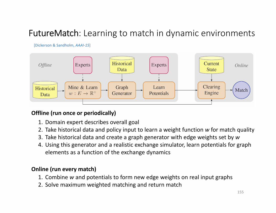
FutureMatch: Learning to match in dynamic environments
155
1. Domain expert describes overall goal 2. Take historical data and policy input to learn a weight function w for match quality3. Take historical data and create a graph generator with edge weights set by w4. Using this generator and a realistic exchange simulator, learn potentials for graph
elements as a function of the exchange dynamics
Offline (run once or periodically)
1. Combine w and potentials to form new edge weights on real input graphs2. Solve maximum weighted matching and return match
Online (run every match)
[Dickerson & Sandholm, AAAI‐15]

Example objective: MaxLife• Maximize aggregate length of time donor organs last in patients …
– … possibly subject to prioritization schemes, fairness, etc …
• Learn survival rates from all living donations since 1987• ~75,000 transplants
• Translate to edge weight
156

• 300+ match runs with real UNOS data• Important to use realistic distribution
157
UNOS(first match run)
UNOS(recent snapshot)

158

Edge weights preprocessed no runtime hit!
• Adjust solver to take potentials into account at runtime
• E.g., P‐O= 2.1 and PO‐AB = 0.1
• Edges between O‐altruist and O‐AB pair has weight:1 – 0.5(2.1+0.1) = ‐0.1
• Chain must be long enough to offset negative weight
• Also take into account learned weight function w
161
Online:

Experimental results
• We show it is possible to:• Increase overall #transplants a lot at a (much) smaller decrease in #marginalized transplants
• Increase #marginalized transplants a lot at no or very low decrease in overall #transplants
• Increase both #transplants and #marginalized
• Sweet spot depends on distribution:• Luckily, we can generate – and learn from – realistic families of graphs!
162

Tutorial outline
• Introduction & preliminaries• Optimization models & state of the practice• Deep dive into dimensions of kidney exchange:
• Short‐term uncertainty• Fairness vs economic efficiency• Long‐term uncertainty & dynamic optimization• Incorporating human expert judgment in better ways• Incentives & mechanism design
• Other organ exchanges• Conclusion & open research problems
168

Transplant centers hide pairs and NDDs from exchange(s)• Why do centers do this?
• Logistical benefit• Money
• What fraction of locally matchable pairs/NDDs do centers hide?• A: 100% [Stewart, Leishman, Sleeman, Monstello, Lunsford, Maghirang, Sandholm, Gentry, Formica,
Friedewald, Andreoni. 2013. American Transplant Congress]
• No mechanism design solution possible in static setting [Roth, Sönmez, Ünver (2007a); Ashlagi, Fischer, Kash, Procaccia, GEB‐13; Ashlagi & Roth (2014)]
• Incentive‐compatible, efficient, long‐term‐IR credit mechanism [Hajaj, Dickerson, Hassidim, Sandholm, Sarne, AAAI‐15]
• Matching favors centers that reveal more than their expected number of pairs/NDDs, and disfavors those who reveal fewer than that
• Supports chains and long cycles• Assumes pairs and NDDs last for only one matching period
169

Mechanism Desiderata
170
(Through the lens of kidney exchange)

Individual rationality (IR)
• Long‐term IR: • In the long‐run, a center will receive at least the same number of matches by participating
• Short‐term IR:• At each time period, a center receives at least the same number of matches by participating
171
Will I be better off participating in the mechanism than I would be otherwise?

Strategy proofness
• In any state of the world …• time period, past performance, competitors’ strategies, current private type, etc
• … a center is not worse off reporting its full private set of pairs than reporting anyother subset
172
Do I have any reason to lie to the mechanism?
No reason to strategize

Efficiency
• Efficiency:• Produces a maximum (i.e. max global social welfare) matching given all pairs, regardless of revelation
• IR‐Efficiency:• Produces a maximum matching constrained by short‐term individual rationality
173
Does the mechanism result in the absolute best possible solution?

The basic kidney exchange game
• Set of n transplant centers Tn = {t1 ... tn}, each with a set of incompatible pairs Vh
• Union of these individual sets is V, which induces the underlying compatibility graph
• Want: all centers participate, submit full set of pairs
• An allocation M is k‐maximal if there is no allocation M' that matches all the vertices in M and also more• Note: k‐efficient → k‐maximal, but not vice versa
[Ashlagi & Roth 2014, and earlier]

Individually rational?
Vertices a1, a2 belong to center a, b1, b2 belong to center b
Center a could match 2 internally By participating, matches only 1 of its own Entire exchange matches 3 (otherwise only 2)
[Ashlagi & Roth 2014, and earlier]
b1 b2
a2a1
Center b
Center a

It can get much worse
Bound is tight
All but one of a's vertices is part of another length kexchange (from different agents)
k‐maximal and IR if amatches his k vertices (but then nobody else matches, so k total)
k‐efficient to match (k‐1)*k
[Ashlagi & Roth 2014, and earlier]
Theorem: For k>2, there exists G s.t. no IR k‐maximal mechanism matches more than 1/(k‐1)‐fraction of those matched by k‐efficient allocation
Example: k=3

Restriction #1
• Proof sketch: construct k‐efficient allocation for each specific hospital's pool Vh
• Repeatedly search for larger cardinality matching in an entire pool that keeps all already‐matched vertices matched (using augmenting matching algorithm from Edmonds)
• Once exhausted, done
Theorem: For all k and all compatibility graphs, there exists an IR k‐maximal allocation
[Ashlagi & Roth 2014, and earlier]

Restriction #2
• Idea: Every 2‐maximal allocation is also 2‐efficient• collection of sets of matched vertices form a matroid
• special independence cases with k=2, also this is a PTIME problem with the |V|3 bipartite augmenting paths matching algorithm
• By Restriction #1, 2‐maximal IR always exists this 2‐efficient IR always exists
•
[Ashlagi & Roth 2014, and earlier]
Theorem: For k=2, there exists an IR 2‐efficient allocation in every compatibility graph

A Dynamic, Credit‐Based Mechanism
179
(That is strategy proof and efficient, if some assumptions hold.)

Dynamic, Credit‐Based Mechanism[Hajaj et al. AAAI‐2015]
• Repeated game• Centers are risk neutral, self interested• Transplant centers have (private) sets of pairs:
• Maximum capacity of 2ki• General arrival distribution, mean rate is ki• Exist for one time period
• Centers reveal subset of their pairs at each time period, can match others internally
180

Credits
• Clearinghouse maintains a credit balance cifor each transplant center over time• High level idea:
• REDUCE ci: center i reveals fewer than expected• INCREASE ci: center i reveals more than expected
• REDUCE ci: mechanism tiebreaks in center i’s favor• INCREASE ci: mechanism tiebreaks against center I
Also remove centers who misbehave “too much.”
181
Credits now matches in the future
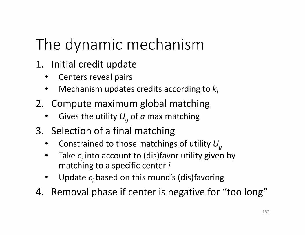
The dynamic mechanism1. Initial credit update
• Centers reveal pairs• Mechanism updates credits according to ki
2. Compute maximum global matching• Gives the utility Ug of a max matching
3. Selection of a final matching• Constrained to those matchings of utility Ug• Take ci into account to (dis)favor utility given by
matching to a specific center i• Update ci based on this round’s (dis)favoring
4. Removal phase if center is negative for “too long”
182

Theoretical guarantees
Theorem: No mechanism that supports cycles and chains can be both long‐term IR and efficient
Theorem: Under reasonable assumptions, the prior mechanism is both long‐term IR and efficient

Experiments on Real Data
184
(Uses data from UNOS exchange, first ~100 match runs)

185

Experiments on Simulated Data
186
(Uses data generated according to [Saidman et al. 2006])

187

This is still a very open problem!
• All models are still limited:• Agency attributed only to transplant centers, not
• Patient‐donor pairs (generally)• Central bodies like a government
• Money?• Most results in the static setting• Determinism• Unreasonable knowledge of agents (e.g., avg. entry)
• Clear policy implications

Competing dynamic matching markets[Das et al. AMMA‐15]
• Dynamic matching markets are typically modeled in isolation, with each agent entering a single market.
• Real‐world applications (e.g kidney exchange) often involve multiple matching platforms drawing from overlapping pools. Questions: • Whether competing platforms increase global loss relative to a single
centralized matching platform. • How does one platform’s matching policy affect global loss in a multi‐
platform setting?
BothNKR only
UNOS only
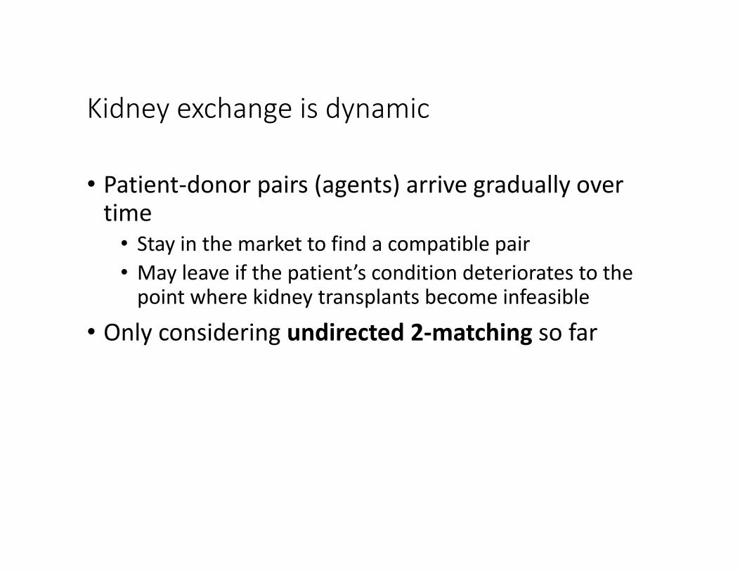
Kidney exchange is dynamic
• Patient‐donor pairs (agents) arrive gradually over time
• Stay in the market to find a compatible pair• May leave if the patient’s condition deteriorates to the point where kidney transplants become infeasible
• Only considering undirected 2‐matching so far

Planner / Clearinghouse platform
• Minimizes the number of agents who perish (leave the exchange without finding a match)
• Knows agent’s expiration time • Has only probabilistic knowledge about future incoming agents
• Selects a subset of acceptable transactions at any point in time

Greedy and patient exchanges[Akbarpour et al., EC‐14]
Greedy algorithm Patient algorithm

Greedy exchange
Greedy algorithm
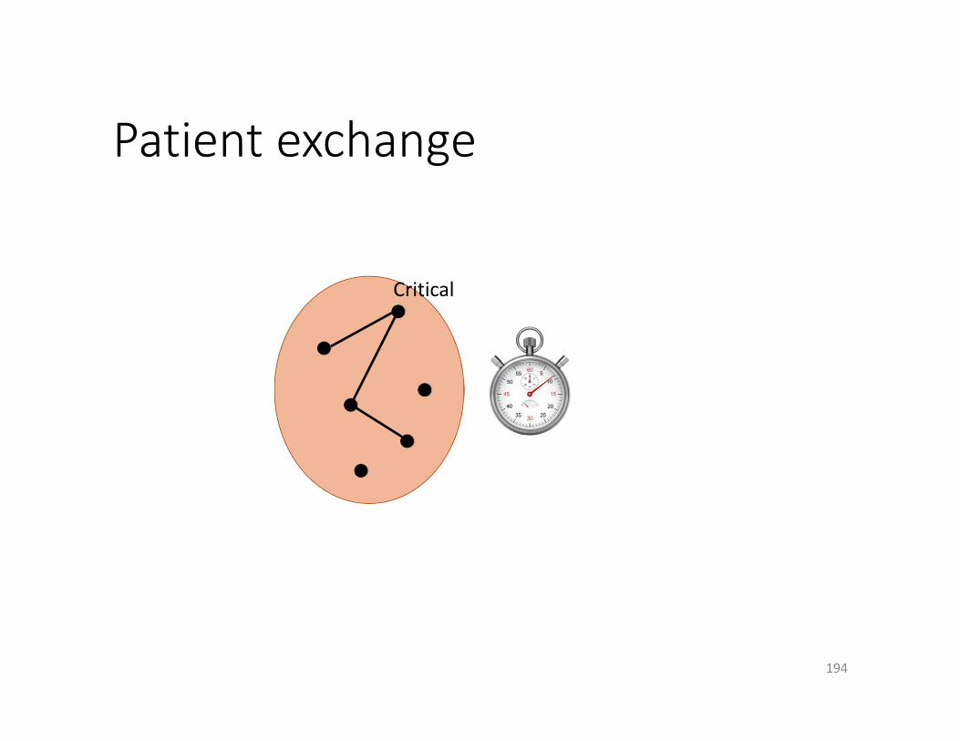
Patient exchange
194
Critical
Patient algorithm

Greedy and patient exchanges
195
≥Loss
Greedy algorithm Patient algorithm
[Akbarpour et al., EC‐14]

Competing exchanges[Das et al. AMMA‐15]
196
How do interactions between overlapping pools, different policies affect social welfare?
Greedy algorithm
Patient algorithm

Model details
• Agents (patient‐donor pairs) arrive at the market according to a Poisson process, with rate parameter m ≥ 1
• The sojourn of an agent is drawn from an exponential distribution, with rate parameter λ = 1
• Pr(acceptable transaction) = d/m, 0 ≤ d ≤ m
197
Average degree of node in graph
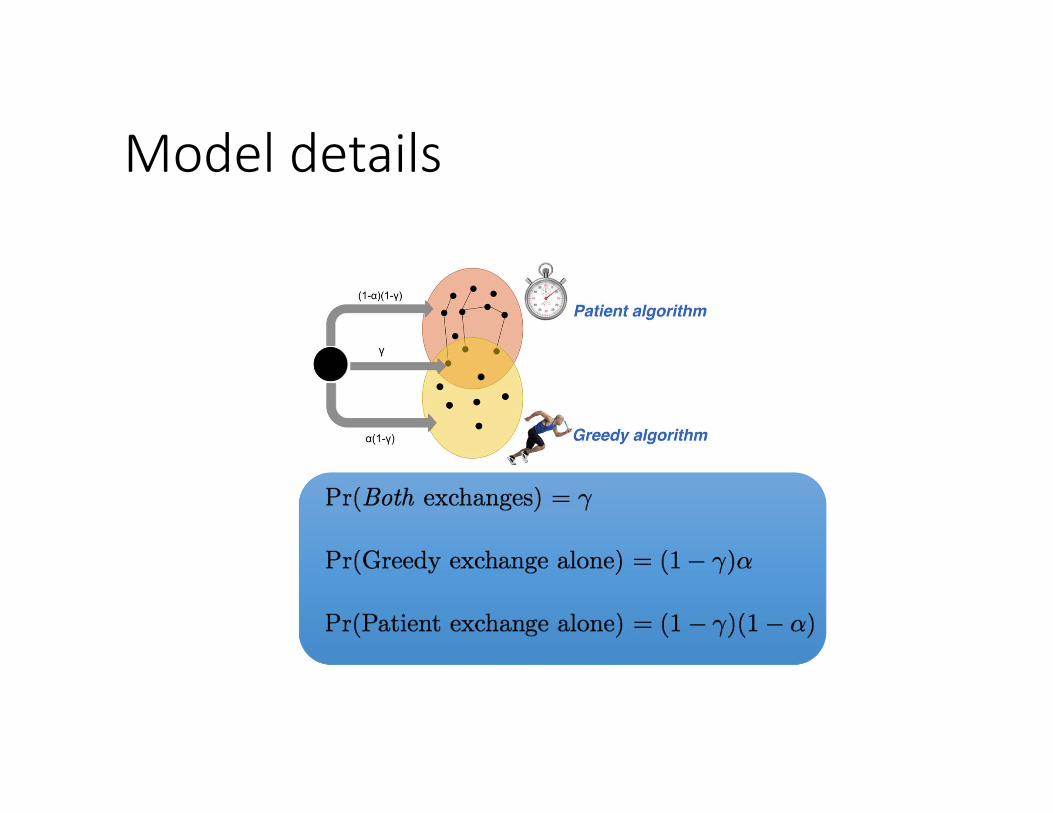
Model details

Three pools

Proof sketch ‐ bound on overall loss
200

Proof sketch ‐ bound on overall loss
2

Expression for overall loss
202
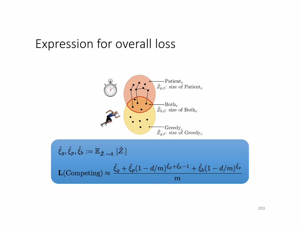
Expression for overall loss
203
Simulation setup
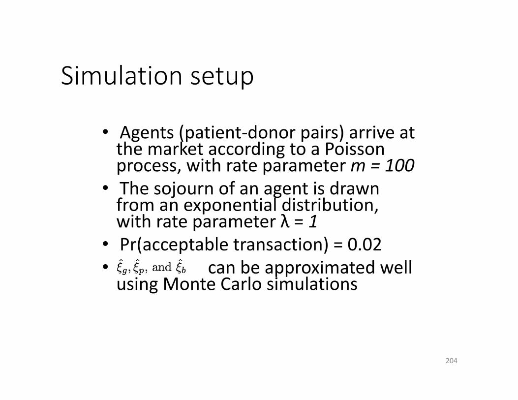
• Agents (patient‐donor pairs) arrive at the market according to a Poisson process, with rate parameter m = 100
• The sojourn of an agent is drawn from an exponential distribution, with rate parameter λ = 1
• Pr(acceptable transaction) = 0.02• can be approximated well using Monte Carlo simulations
204

Simulation results
205

Kidney exchange experiments
• Edges are determined by medical characteristics (Pr(acceptable transac on) ≠ d/m)
UNOS (Real patient profiles)SAIDMAN (Simulated patient profiles)
• Can incorporate longer cycles, chains, etc.We consider 2‐ and 3‐cycles
206

Experimental results
207
Experiment Simulation

Experimental results
208

Problem still very open, very relevant!• Relax assumptions:
• agents select subset of platforms to enter• platforms select matching policy• 2‐ vs 3‐cycles, chains?
• Bounds on loss: generalize, tighten, n > 2 platforms
209

Tutorial outline
• Introduction & preliminaries• Optimization models & state of the practice• Deep dive into dimensions of kidney exchange:
• Short‐term uncertainty• Fairness vs economic efficiency• Long‐term uncertainty & dynamic optimization• Incorporating human expert judgment in better ways• Incentives & mechanism design
• Other organ exchanges• Conclusion & open research problems
210

Moving beyond kidneys: Livers[Ergin, Sönmez, Ünver w.p. 2015]
• Similar matching problem (mathematically)
• Right lobe is biggest but riskiest; exchange may reduce right lobe usage and increase transplants
[Sönmez 2014]

• Fundamentally different matching problem• Two donors needed
Moving beyond kidneys: Lungs[Ergin, Sönmez, Ünver w.p. 2014]
[Date et al. 2005; Sönmez 2014]
(Compare to the single configuration for a “3‐cycle” in kidney exchange.)

Mechanism design: Lung exchange [Luo & Tang IJCAI‐15]
Theorem: Even the problem of finding a non‐empty feasible swap is NP‐hard
(Reduction from 3D‐Matching)
They give a Pareto‐efficient, IR, IC mechanism for the static setting
(where the agents are patient‐donor‐donor triples, not the transplant centers)

Moving beyond a single organ
• Chains are great! [Anderson et al. 2015, Ashlagi et al. 2014, Rees et al. 2009]• Kidney transplants are “easy” and popular:
• Many altruistic donors
• Liver transplants: higher mortality, morbidity:• (Essentially) no altruistic donors
A
D1
P1
D2
P2
D3
P3
D4
P4
…
[Dickerson Sandholm AAAI‐14, JAIR‐2016]

Would this help?
• Theory: adapted Erdős‐Rényi models• Dense model [Saidman et al. 2006]
• Constant probability of edge existing• Less useful in practice [Ashlagi et al. 2012, Ashlagi Jaillet Manshadi 2013]
• Sparse model [Ashlagi et al. 2012]• 1‐λ fraction is highly‐sensitized (pH = c/n)• λ fraction is lowly‐sensitized (pL > 0, constant)
• Not all kidney donors want to give livers• Constant probability pKL > 0
215
[Dickerson Procaccia Sandholm 2013, 2014]
Sparse graph, many altruists
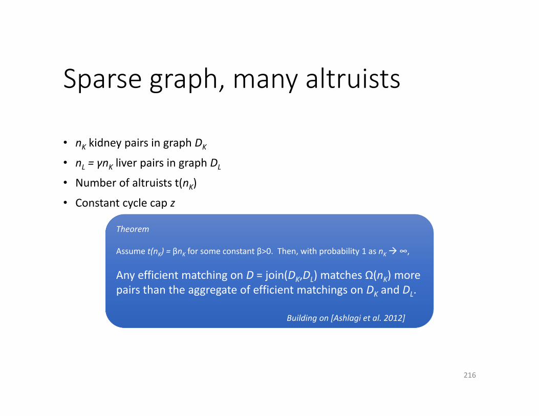
• nK kidney pairs in graph DK
• nL = γnK liver pairs in graph DL
• Number of altruists t(nK)
• Constant cycle cap z
216
Theorem
Assume t(nK) = βnK for some constant β>0. Then, with probability 1 as nK∞,
Any efficient matching on D = join(DK,DL) matches Ω(nK) more pairs than the aggregate of efficient matchings on DK and DL.
Building on [Ashlagi et al. 2012]

Intuition• Find a linear number of “good cycles” in DL that are length > z
• Good cycles = isolated path in highly‐sensitized portion of pool and exactly one node in low portion
• Extend chains from DK into the isolated paths (aka can’t be matched otherwise) in DL, of which there are linearly many• Have to worry about pKL, and compatibility between vertices
• Show that a subset of the dotted edges below results in a linear‐in‐number‐of‐altruists max matching
• linear number of DK chains extended into DL• linear number of previously unmatched DL vertices matched
217
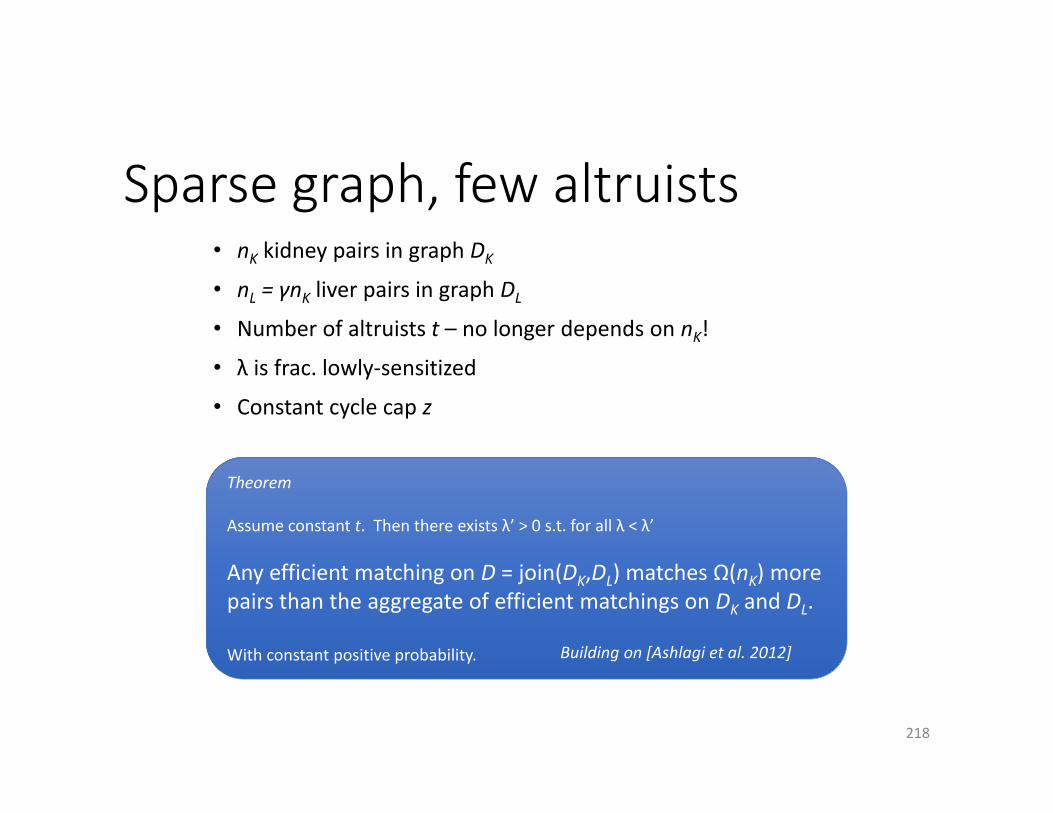
Sparse graph, few altruists• nK kidney pairs in graph DK
• nL = γnK liver pairs in graph DL
• Number of altruists t – no longer depends on nK!
• λ is frac. lowly‐sensitized
• Constant cycle cap z
218
Theorem
Assume constant t. Then there exists λ’ > 0 s.t. for all λ < λ’
Any efficient matching on D = join(DK,DL) matches Ω(nK) more pairs than the aggregate of efficient matchings on DK and DL.
With constant positive probability. Building on [Ashlagi et al. 2012]
Intuition
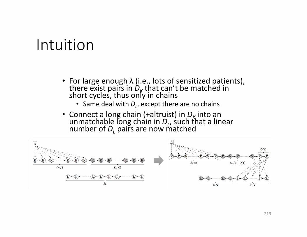
• For large enough λ (i.e., lots of sensitized patients), there exist pairs in DK that can’t be matched in short cycles, thus only in chains
• Same deal with DL, except there are no chains• Connect a long chain (+altruist) in DK into an unmatchable long chain in DL, such that a linear number of DL pairs are now matched
219

Dense graph, many altruists
Take efficient matching on the kidney exchange graph alone, extend a linear number of chains into the leftover pairs after an efficient matching in the liver exchange alone.
220

FutureMatch + multi‐organ exchange?
• Combination results in• Linear gain in theory• Big gains in simulation
• Equity problems• Kidneys ≠ livers• Hard to quantify cross‐organ risk vs. reward
221
Let FutureMatchsort it out?
Tutorial outline
• Introduction & preliminaries• Optimization models & state of the practice• Deep dive into dimensions of kidney exchange:
• Short‐term uncertainty• Fairness vs economic efficiency• Long‐term uncertainty & dynamic optimization• Incorporating human expert judgment in better ways• Incentives & mechanism design
• Other organ exchanges• Conclusion & open research problems
222

Conclusions• Kidney exchanges are a broadly fielded success for AI• Powered by scalable, flexible batch solvers• Open chains are powerful• Real kidney exchanges have cycles, chains, weights, arrivals/departures, edge failures, fairness
considerations, human value judgments, …
• Dynamic problem• General‐purpose trajectory‐based online algorithms• General purpose idea of how to use “potentials” to capture the future into batch optimization• Both leverage distributional information and our offline algorithm• Both outperform batch‐based approach
• Failure‐aware probabilistic matching• Fairness• Futurematch: learning to do generalized matching in complex settings• Centers hide pairs; impossibility results for static settings, but “credit” mechanisms work• Liver lobes, multi‐organ, lung parts, …
223

Future research• Work on real problem: 2‐ and 3‐cycles, chains, dynamics, edge failures• We recently open‐sourced the most realistic organ‐exchange simulator• Still lots to be done
• Even faster algorithms, esp. with chains• Better dynamic algorithms that handle arrivals and departures; can one improve
more than 10% over batch approach?• E.g., potentials based on more donor and patient features [we’re working on this]
• Better failure‐aware algorithms• Better edge testing policies [we’re working on this]• Matching cadence: Race to bottom among exchanges
[Das, Dickerson, Li, Sandholm, AMMA‐15]• Better incentive schemes
• Credit scheme [Hajaj, Dickerson, Hassidim, Sandholm, Sarne, AAAI‐15]• Multi‐donor kidney exchange [we’re working on this]• Other organs
• Liver & cross‐organ exchange [Dickerson & Sandholm, GREEN‐COPLAS‐13, AAAI‐14]• Lung “components” [Ergin, Sönmez, Ünver, draft 2014‐15; Tang et al. 2015]
225

Future work regarding fielding• Getting dynamic and failure‐aware approach fielded• Better crossmatch prediction• Better edge testing policies • Getting credit schemes fielded• Better donor pre‐select tools• Insurance to pay for testing, etc.• International exchange• Exchanges beyond kidneys• In the US: Shutting down sniping manual private exchanges, and having one system (as there is for deceased donors)
226