Embed Size (px)
Citation preview
Mathematical Methods in Biology and
Neurobiology
Jurgen Jost1
January 23, 2007
1Max Planck Institute for Mathematics in the Sciences, Inselstr.22, 04103 Leipzig,
Germany, [email protected]
Copyright by the author. No reproduction or distribution without the author’s per-
mission

2
Contents
1 Introduction 5
1.1 Theses about biology . . . . . . . . . . . . . . . . . . . . . . . . . 51.2 Fundamental biological concepts . . . . . . . . . . . . . . . . . . 61.3 A classification of mathematical methods . . . . . . . . . . . . . 6
2 Discrete structures 9
2.1 Graphs and networks . . . . . . . . . . . . . . . . . . . . . . . . . 92.1.1 Graphs in biology . . . . . . . . . . . . . . . . . . . . . . 92.1.2 Definitions and qualitative properties . . . . . . . . . . . 102.1.3 The graph Laplacian and its spectrum . . . . . . . . . . . 13
2.2 Descendence relations . . . . . . . . . . . . . . . . . . . . . . . . 232.2.1 Trees and phylogenies . . . . . . . . . . . . . . . . . . . . 232.2.2 Genealogies (pedigrees) . . . . . . . . . . . . . . . . . . . 342.2.3 Gene genealogies (coalescents) . . . . . . . . . . . . . . . 35
3 Stochastic processes 41
3.1 Random variables . . . . . . . . . . . . . . . . . . . . . . . . . . . 413.2 Random processes . . . . . . . . . . . . . . . . . . . . . . . . . . 463.3 Poisson processes and neural coding . . . . . . . . . . . . . . . . 473.4 Branching processes . . . . . . . . . . . . . . . . . . . . . . . . . 533.5 Random graphs . . . . . . . . . . . . . . . . . . . . . . . . . . . . 59
4 Pattern formation 67
4.1 Partial differential equations . . . . . . . . . . . . . . . . . . . . . 674.2 Diffusion and random walks . . . . . . . . . . . . . . . . . . . . . 804.3 Dynamical systems . . . . . . . . . . . . . . . . . . . . . . . . . . 89
4.3.1 Systems of ordinary differential equations . . . . . . . . . 894.4 Reaction-diffusion systems . . . . . . . . . . . . . . . . . . . . . . 106
4.4.1 Reaction-diffusion equations . . . . . . . . . . . . . . . . . 1064.4.2 Travelling waves . . . . . . . . . . . . . . . . . . . . . . . 1114.4.3 Reaction-diffusion systems . . . . . . . . . . . . . . . . . . 1134.4.4 The Turing mechanism . . . . . . . . . . . . . . . . . . . 119
4.5 Continuity and Fokker-Planck equations . . . . . . . . . . . . . . 126
3

4 CONTENTS
Chapter 1
Introduction
1.1 Theses about biology
Thesis 1. Biological structures are aggregate structures. Therefore, biologicallaws are not basic ones that do not admit exceptions, but rather emerging fromsome lower scale.
Thesis 2. Biological processes intertwine stochastic effects and deterministicdynamics. Randomness can support order while deterministic processes can beunpredictable, chaotic. The question then is at which level regularities emerge.
Thesis 3. Large populations of discrete units can be described by continuousmodels and, conversely, invariant discrete quantities can emerge from an un-derlying continuous substrate.
Thesis 4. Fundamental biological concepts, like fitness or information, are rel-ative and not absolute ones.
Thesis 5. Fundamental biological quantities do not satisfy conservation laws.Those rather appear as external constraints.
Thesis 6. Biological systems interact with their environments and are ther-modynamically open. Biological structures sustain the processes that reproducethem and are therefore operationally closed.
Thesis 7. Biological structures are results of historical processes. It is the taskof biological theory to distinguish the regularities from the contingencies.
Thesis 8. The abstract question posed to mathematics by biology is the oneof structure formation. This needs to be understood as a process because livingstructures are not at thermodynamic equilibrium.
Thesis 9. Gathering biological data without guiding concepts and theories isuseless.
5
6 CHAPTER 1. INTRODUCTION
1.2 Fundamental biological concepts
1. The gene is the unit of coding, function, and inheritance. As such, it linksmolecular biology and evolutionary biology. The Neodarwinian Synthesiscombined Mendel and Darwin. Modern molecular biology seems to offera more basic perspective.
2. The cell is the unit of metabolism. It constitutes the basic operationallyclosed, autopoietic system in biology. Modern biology struggles to under-stand the cell on the basis of their molecular constituents, DNA, RNA,and polypeptides (proteins). Multicellular organisms emerge through apartial suppression of the autonomy of the constituting cells.
3. The species represents the balance between the diverging effects of ge-netic mutations and selection at the organismic or other levels and theconverging mechanism of sexual recombination. It is the arena of popu-lation biology, a child of the Neodarwinian Synthesis and the first successof mathematical models in biology. It is also important in ecology.
The organism, in fact, is the carrier of genes, the organisation of cells, and themember of a species. It thus links the three fundamental biological concepts. Itis also a, but not the exclusive, unit of selection.It seems that neurobiology has not yet identified such a fundamental concept,but perhaps the spike can be considered as the basic event of informationtransmission, and the synapse as the basic structure supporting this.
1.3 A classification of mathematical methods
1. Discrete structures → Algebra
(a) Static structures
i. Algebraic concepts: Combination and composition of objects
ii. Graphs and networks, including phylogenetic trees
iii. Information
iv. Discrete invariants of continuous structures and dynamical pro-cesses
(b) Discrete processes (Cellular automata, Boolean networks, finite statemachines,...)
(c) Game theory as the formalisation of competition
2. Continuous methods → Analysis
(a) Deterministic dynamical processes
i. Continuous states enable phase transitions and bifurcations, thatis, qualitative structural changes resulting from small underlyingvariations

1.3. A CLASSIFICATION OF MATHEMATICAL METHODS 7
ii. Continuous states and time: Ordinary differential equations andother dynamical systems
iii. Continuous spatial structures: Partial differential equations (ex-ample: Reaction-diffusion equations)
(b) Stochastic analysis
i. Stochastic processes (while stochastic processes may also operateon discrete quantities, the concept of probability is a continuousone)
ii. Population processes: averaging over stochastic fluctuations inlower level dynamics
iii. Optimisation schemes with stochastic ingredients: Genetic andother evolutionary algorithms, swarm algorithms for distributedsearch, certain neural networks,...
iv. Statistical methods for the analysis of biological data
3. Hybrid models
(a) Difference equations (continuous states, but discrete time)
(b) Dynamical networks (dynamical systems coupled by a graph), in par-ticular neural networks
4. System theory as a global unifying perspective?
According to the preceding list that not all mathematical subjects seem tobe relevant for biology. Classical algebraic structures occur in a cursory mannerat best, and one of the deepest branches, number theory and arithmetics, is en-tirely absent. Also, the third area of mathematics besides algebra and analysis,namely geometry, is entirely missing in our list. This does not mean that it isirrelevant in a similar manner as number theory is because its objects are notfound in biology, but rather that it plays only a somewhat subordinate role incomparison with analysis and discrete mathematics. Organisms and their con-stitutive biological structures like cells are living and interacting in space, andare defining and shaping their own spaces like architectural structures which isconstitutive for morphology. Symmetries and invariances, the merging groundof algebra and geometry, are important issues for the neurobiology underlyingcognition. as well as for many classification purposes. One can, of course, alsoconsider more abstract spaces of relationships, like state spaces in dynamicalsystems. Thus, there is some role for geometry after all.

8 CHAPTER 1. INTRODUCTION
Chapter 2
Discrete structures
2.1 Graphs and networks
2.1.1 Graphs in biology
A graph is the mathematical structure representing binary relationships betweendiscrete elements. These elements are the vertices of the graph, and the rela-tionships are encoded as connections or edges between vertices. Such a graphcan then be a network, that is, the substrate of dynamical interactions carriedby the edges between processes located at the vertices. Biological applicationsabound.In neural networks, the vertices stand for neurons, and the edges for synapticconnections between them. The interaction is the electrochemical transmissionof pulsed dynamical activity, the spikes generated in the neurons. This activ-ity is considered to be the carrier of information, enabling cognitive processes,but the precise identification of the information inside that dynamical activityremains unclear at present.At smaller scales, the vertices can represent molecules like proteins, and theedges again interactions between them. The vertices can also stand for genes,and the edges for correlations in expression patterns indicating functional inter-actions.At larger scales, the vertices can be the members of a population, and the edgessocial or other interactions, like mating. For a population with separate sexes,we then have a bipartite graph, that is, one with two distinct classes of elementssuch that edges exist only between members of opposite classes, but not insideone class.At the still larger scale of ecosystems, the vertices can represent species, andthe edges stand for trophic interactions. The graph then encodes a foodweb.
Another important class of biological graphs are the phylogenetic trees thatturn genetic or other similarities between species into descendence relationsfrom common ancestors. For individual descendence relations inside a sexually
9
10 CHAPTER 2. DISCRETE STRUCTURES
recombining species we rather have pedigrees because each individual then hastwo parents which in turn may have more than one offspring.
2.1.2 Definitions and qualitative properties
We now display some formal definitions and start with the simplest situation.A graph Γ is a pair (V,E) of a finite set V of vertices or nodes and a set E ofunordered pairs, called edges or links, of different elements of V (and we assumeE 6= ∅ to make the graph nontrivial). Thus, when there is an edge e = (i, j)for i, j ∈ V , we say that i and j are connected by the edge e and that they areneighbours, i ∼ j. Defining edges as unordered pairs of vertices means that weconsider (i, j) and (j, i) as the same pair. Thus, the neighborhood relation issymmetric. Requiring that the vertices connected by an edge be different thenmeans that there are no edges connecting a vertex to itself. Thus, the neigh-borhood relation is not reflexive. In general, it is not transitive either, that is,i ∼ j and j ∼ k need not imply i ∼ k. The degree ni of the vertex i is thenumber of its neighbours. Also, the order |Γ| is the number of vertices in Γ, i.e.,the cardinality of the vertex set V .So far, we are assuming that the edges are undirected, that is, the edge (i, j)is the same as (j, i). One may, naturally, also consider directed graphs, that is,where an edge e = (i, j) is considered to go from i to j rather than connect i andj in a symmetric manner. For example, this is appropriate for formalize neuro-biological networks because synapses between neurons are directed, starting atthe presynaptic neuron and going to the postsynaptic one. In addition, synapsesahve strengths or weights, and so, we can also consider weighted graphs whereeach edge e carries a weight or label we that indicates its strength. In fact, wemay then also allow that some of the weights are negative. In a neural network,an edge with a negative weight would represent an inhibitory synapse.Of course, every unweighted graph becomes a weighted one by assigning theweight 1 to every edge. An undirected graph with positive weights becomesa metric space by identifying each edge e with the interval of length (we)
−1.In particular, an unweighted graph then is a metric space where each edge isisometric to the unit interval. The distance between vertices then equals thelength of the shortest path joining them. In particular, neighbors in the graphhave distance 1.We shall start with undirected and unweighted graphs as the simplest case. Inthe definition, we require that our graphs Γ be finite, a biologically directlyplausible assumption. Moreover, we shall assume, unless stated to the contrary,that they are connected. That means that for every pair of distinct vertices i, jin Γ, there exists a path between them, that is, a sequence i = i0, i1, . . . , im = jof distinct vertices such that iν−1 ∼ iν for ν = 1, . . . ,m. Since we can de-compose graphs that are not connected into their connected components, theconnectivity assumption is no serious restriction.An obvious way of representing a graph Γ with vertices i = 1, . . . , N is providedby its adjacency matrix A = (aij). In the unweighted case, we put aij = 1when there is an edge from i to j and = 0 else. We have aii = 0 because we
2.1. GRAPHS AND NETWORKS 11
exclude self-loops of vertices, and Γ is undirected iff aij = aji for all i, j. Inthe weighted case, we simply put aij = wij , the weight of the edge from i to j.Of course, most large graphs arising in applications are sparse, that is, betweenmost pairs i, j, there is no edge. This means that most of the entries of theadjacency matrix are 0. Therefore, that matrix does not provide a very efficientway of encoding the graph. A more efficient way is provided by simply listingfor each i those vertices that send links to i, together with the correspondingweights in the weighted case.
An isomorphism between graphs Γ1 = (V1, E1),Γ2 = (V2, E2) is a bijectionΦ : V1 → V2 that preserves neighborhood relations, that is, i ∼ j iff Φ(i) ∼ Φ(j).In other words, i and j are connected by an edge precisely if their images underΦ are. Isomorphisms preserve the degrees of vertices, that is, ni = nΦ(i) forevery vertex i. An automorphism of Γ is an isomorphism from Γ onto itself.The identity map of the vertex set of Γ is obviously an automorphism, but theremay or may not be others, depending on the structure of Γ. The automorphismsof Γ form a group under composition. We can then quantify the symmetry ofΓ as the order of its automorphism group.The number of graphs of order k grows very fast as a function of k, and there-fore, it becomes unwieldy already for rather small k to list all graphs of order k.Therefore, it is of interest to develop constructions for particular classes or typesof graphs. There exist deterministic and stochastic construction schemes. Weshall discuss stochastic constructions below in 3.5 in the chapter on stochasticprocesses. Deterministic constructions typically produce rather regular graphs,that is ones with high degrees of symmetries whereas the stochastic construc-tions can produce typical representatives of larger classes of graphs. A paradigmof a symmetric graph is a complete graph, meaning that any two different ver-tices are connected by an edge. For a complete graph, every bijection of itsvertices yields an automorphism, and therefore, it is maximally symmetric.A cycle in Γ is a closed path i0, i1, . . . , im = i0 for which all the vertices i1, . . . , imare distinct. For m = 3, we speak of a triangle. A cycle that contains all thevertices of Γ is called a Hamiltonian cycle (and such a cycle need not exist fora given graph). A graph without cycles is called a tree.A graph is called k-regular if all vertices have the same degree k. As alreadymentioned, a graph is bipartite if its vertex set can be decomposed into two dis-joint components V1, V2 such that whenever i ∼ j, then i and j are in differentcomponents. It is not hard to see that a graph is bipartite iff it does not containcycles of odd length. In particular, it cannot contain any triangles.Another useful concept for analyzing graphs is the k-core. For k ∈ N, the k-coreof a graph Γ is the not necessarily connected maximal subgraph H of Γ with theproperty that every vertex of H has at least k neighbors in H , that is, its degreein H is at least k. When we exclude the trivial case of an isolated vertex, thenΓ itself conincides with its 1-core. When Γ is a tree, already its 2-core is empty.Every cycle of Γ is contained in its 2-core. The core decomposition of Γ, that is,the successive determination of its k-cores for increasing k, is a computationallysimple way of decomposing the graph.
12 CHAPTER 2. DISCRETE STRUCTURES
There exist other parameters that describe certain – more or less – importantqualitative properties of graphs. One set of such parameters arises from themetric on the graph generated by the above assignment of length 1 to everyedge. The diameter of the graph is the maximal distance between any two ofits nodes. As an example how such a parameter can distinguish between typicaland non-typical, special graphs, we record that there exists a constant c with theproperty that the fraction of all graphs with N nodes having diameter exceedingc logN tends to 0 for N → ∞. Informally expressed, most graphs of N nodeshave a diameter of order logN . Thus, graphs with large diameters, like a chaini1 ∼ i2 ∼ · · · ∼ iN with no other edges, are rare. In the other direction, thatis, considering graphs with very small diameters, of course, a fully connectedgraph has diameter 1. However, one can realize a small diameter already withmuch fewer edges; namely, one selects one central node to which every othernode is connected. In that manner, one obtains a graph of N nodes with N − 1edges and diameter 2. Of course, the central node then has a very large degree,namely N − 1. It is a big hub. Similarly, one can construct graphs with a fewhubs, so that none of them has to be quite that big, efficiently distributed sothat the diameter is still rather small. Such graphs can be realized as so-calledscale free graphs to be discussed below. Another useful quantity is the averagedistance between nodes in the graph. The property of having a small diameteror average distance has been called the small-world effect.A rather different quantity is the clustering coefficient that measures how manyconnections there exist between the neighbors of a node. Formally, it is definedas
C :=3 × number of triangles
number of connected triples of nodes. (2.1.1)
The normalization is that C becomes one for a fully connected graph. It vanishesfor trees and other bipartite graphs.A triangle is a cycle of length 3. One may then also count the number of cyclesof length k, for integers > 3. A different generalization consists in consideringcomplete subgraphs of order k. Here, the complete k-graph is the graph with kvertices and links between all i 6= j. A k-clique in a graph Γ is a subgraph that isa complete k-graph. For example, for k = 4, we would have a subset of 4 nodesthat are all mutually connected. One may then associate a simplicial complexto our graph by assigning a k-simplex to every such complete subgraph, withobvious incidence relations. For example, two such k-simplices share a (k − 1)-dimensional face and are called adjacent when the two corresponding completek-subgraphs have a complete (k − 1)-graph in common. This is the basis oftopological combinatorics, enabling one to apply tools from simplicial topologyto graph theory.A basic question in the analysis of graphs is the cluster decomposition. Thatmeans that we try to find subgraphs, the clusters, that are densely connectedinside, but only sparsely connected to the rest of the graph. For example,one can try to disconnect the graph by cutting as few edges as possible, toobtain two large (super)clusters, and then perhaps iterate the process inside
2.1. GRAPHS AND NETWORKS 13
these superclusters to find a finer decomposition. Conversely, one can try tobuild up the clusters from inside, for example by identifying maximal sets ofadjacent k-cliques, or, equivalently, in the simplicial complex defined above,finding maximal sets of k-simplices that are connected by (k − 1)-dimensionalfaces. Here, the clusters found are typically not disjoint, in contrast to the onesobtained by the edge-cutting methods. Of course, one may then analyze theoverlap between those clusters.Concerning the number of edges needed to disconnect a graph, some insight isprovided by the following result of Menger:
Lemma 2.1.1. Let V1 and V2 be disjoint subsets of the vertex set of a graphΓ = (V,E). The minimal number of edges that need to be deleted from Γ in orderto disconnect it in such a manner that V1 and V2 are in different components isequal to the maximum number of edge-disjoint paths (that is no two paths areallowed to have an edge in common, even though they may well pass through thesame vertex) with one endpoint in V1 and the other in V2.
Another general question is to identify the most important “core” of thegraph. The k-core defined above is one useful concept for that. The idea thereis that a node is important when it is connected with other important nodes.Thus, one finds the core by successively deleting the less important nodes. Thatprocedure might make some nodes that have originally been highly connected,that is, have a large degree, less relevant, because they had only been connectedto other nodes of low degrees. Therefore, in particular, the degree of a nodein general is not a good measure of its importance. One can also quantify theimportance of a vertex or an edge by counting how many shortest connectionsbetween pairs of nodes pass through them. Again, one should be a bit cautioushere because in some cases, there exist alternatives to shortest paths that arenot substantially longer but that avoid the vertex or edge in question. In otherwords, sometimes vertices or edges can easily be replaced as parts of shortconnections while in other cases that may not possible. When one decides theimportance according to such considerations, this effect should also be takeninto account.
2.1.3 The graph Laplacian and its spectrum
As before, Γ is a finite and connected graph. Probably the most powerful andcomprehensive set of invariants comes from the spectrum of the graph Laplacianof Γ to which we now turn. (In general terms, this means that, in order toanalyze a graph Γ, we shall study functions defined on Γ. These functionswill then be decomposed in terms of a particular set of basis functions, as inFourier analysis. From those basis functions, we shall obtain spectral valuesthat incorporate the characteristic properties of Γ.)There are several non-equivalent definitions of the graph Laplacian employed inthe literature. In order to clarify this issue, we assign weights bi(> 0) to the
14 CHAPTER 2. DISCRETE STRUCTURES
vertices1 and introduce an L2-product for (complex-valued) functions on Γ:
(u, v) :=∑
i∈Vbiu(i) ¯v(i). (2.1.2)
(Since we shall only consider real operators below, it suffices to consider realvalued functions, and then the complex conjugate in (2.1.2) is not relevant.)The most natural choices are bi = 1 or bi = ni where ni is the degree of thevertex i.2 We may then choose an orthonormal base of that space L2(Γ). Inorder to find such a basis that is also well adapted to dynamical aspects, westudy the graph Laplacian
∆ : L2(Γ) → L2(Γ)
∆v(i) :=1
bi(∑
j,j∼iv(j) − niv(i)) (2.1.3)
where j ∼ i means that j is a neighbor of i.3
We, in contrast to much of the literature on graph theory (see e.g. [14]), but inaccordance with [5], prefer the weights bi = ni over bi = 1 because the formerare well adapted to random walks and conservation laws. (When we have aparticle randomly moving on a graph with step size 1 then when it is at vertex iit can choose each of the neighbors of i with probability 1/ni for its next move,and this leads to the corresponding factor in the Laplace operator underlyingthat random walk.)The idea behind the definition of ∆ is of course that one compares the value ofa function v at a vertex i with the average of the values at the neighbors of i.When that average is larger than the value at i, we have (∆v)(i) > 0.The important properties of ∆ are the following ones:
1. ∆ is selfadjoint w.r.t. (., .):
(u,∆v) = (∆u, v) (2.1.4)
for all u, v ∈ L2(Γ).4 This holds because the neighborhood relation issymmetric.
1These vertex weights should not be confused with the edge weights discussed above; inother words, here, we are not considering weighted graphs in the sense defined above.
2For purposes of normalization, one might wish to put an additional factor N in front ofthe product where N is the number of elements of the graph or, equivalently, divide all thevertex weights by N , but we have decided to omit that factor in our conventions .
3There are several different definitions of the graph Laplacian in the literature. Some ofthem are equivalent to ours inasmuch as the yield the same spectrum, but others are not. Thereason is simply that the weights in the underlying product are chosen differently. The operatorLv(i) := niv(i)−P
j,j∼i v(j) that is often employed in the literature corresponds to the weights
bi = 1 (up to the minus sign, of course). The operator Lv(i) := v(i) − P
j,j∼i1
√ni
√nj
v(j)
employed in the monograph [5], apart from the minus sign, has the same eigenvalues as ∆ forthe weights bi = ni: if ∆v(i) = µv(i), then w(i) =
√niv(i) satisfies Lw(i) = −µw(i).
4An operator A = (Aij) is symmetric w.r.t. a product 〈v, w〉 :=P
i biv(i) ¯w(i), that is,〈Av, w〉 = 〈v, Aw〉 if biAij = bjAji for all indices i, j. The bi are often called multipliers inthe literature.
2.1. GRAPHS AND NETWORKS 15
2. ∆ is nonpositive:(∆u, u) ≤ 0 (2.1.5)
for all u. This follows from the Cauchy-Schwarz inequality.
3. ∆u = 0 precisely when u is constant. This one sees by observing that,when ∆u = 0, there can neither be a vertex i with u(i) ≥ u(j) for allj ∼ i with strict inequality for at least one such j, that is, a nontriviallocal maximum, nor a nontrivial local minimum, as this would contradictthe fact that ∆u(i) = 0 means that the value u(i) is the average of thevalues at the neighbors of i. Since Γ is connected, u then has to be aconstant (when Γ is not connected, a solution of ∆u = 0 is constant onevery connected component of Γ.)
The preceding properties have consequences for the eigenvalues of ∆:
• By 1, the eigenvalues are real.
• By 2, they are nonpositive. We write them as −λk so that the eigenvalueequation becomes
∆uk + λkuk = 0. (2.1.6)
• By 3, the smallest eigenvalue is λ0 = 0. Since we assume that Γ is con-nected, this eigenvalue is simple, that is
λk > 0 (2.1.7)
for k > 0 where we order the eigenvalues as
λ0 = 0 < λ1 ≤ ... ≤ λK
where we put K := N − 1.
We next consider, for neighbors i, j,
Du(i, j) := u(i) − u(j). (2.1.8)
D can be considered as a map from functions on the vertices of Γ to functions onthe edges of Γ. In order to make the latter space also an L2-space, we introducethe product
(Du,Dv) :=∑
e=(i,j)
(u(i) − u(j))(v(i) − v(j)). (2.1.9)
Note that we are summing here over edges, and not over vertices. If we didthe latter, we would need to put in a factor 1/2 because each edge would thenbe counted twice. We also point out that in contrast to the product of (2.1.2),(u, v) =
∑
i biu(i)v(i), we do not include weights here. The reason is that herethe sum should be considered as a sum of edges and not one over vertices, andsince we are considering unweighted graphs at this point, the edges do not carryany natural weights.
16 CHAPTER 2. DISCRETE STRUCTURES
The product (2.1.9) encodes more information about the graph than the product(2.1.2). The latter only depends on the weights, but not on the connectionstructure of the graph. There exist many structurally quite diverse graphs withthe same weight sequence, and given a graph, one can rewire it by a crossexchange of edges without changing the degrees of the nodes. Namely, givenvertices i1 ∼ j1 and i2 ∼ j2, but without edges between i1 and i2, nor betweenj1 and j2, we create a new graph by deleting the edges between i1 and j1 andbetween i2 and j2 and inserting new edges between i1 and i2 and between j1and j2. That operation preserves the degrees of all vertices, and therefore alsothe product (2.1.2) for any functions u, v on the graph. (2.1.9), in contrast, isaffected because the edge set is changed.We have
(Du,Dv) =∑
i
1
2(niu(i)v(i) +
∑
j
nju(j)v(j) − 2∑
j∼iu(i)v(j))
= −∑
i
u(i)∑
j∼i(v(j) − v(i))
= −(u,∆v). (2.1.10)
Thus, our product (2.1.9) is naturally related to the Laplacian ∆.We may find an orthonormal basis of L2(Γ) consisting of eigenfunctions of ∆,
uk, k = 0, ...,K
(K = N − 1). This is achieved as follows. We iteratively define, with H0 :=H := L2(Γ) being the Hilbert space of all real-valued functions on Γ with thescalar product (., .),
Hk := v ∈ H : (v, ui) = 0 for i ≤ k − 1, (2.1.11)
starting with a constant function u0 as the eigenfunction for the eigenvalueλ0 = 0. Also
λk := infu∈Hk−0
(Du,Du)
(u, u), (2.1.12)
that is, we claim that the eigenvalues can be obtained as those infima. First ofall, since Hk ⊂ Hk−1, we have
λk ≥ λk−1. (2.1.13)
Secondly, since the expression in (2.1.12) remains unchanged when a function uis multiplied by a nonzero constant, it suffices to consider those functions thatsatisfy the normalization
(u, u) = 1 (2.1.14)
whenever convenient.We may find a function uk that realizes the infimum in (2.1.12), that is
λk =(Duk, Duk)
(uk, uk). (2.1.15)
2.1. GRAPHS AND NETWORKS 17
Since then for every ϕ ∈ Hk, t ∈ R
(D(uk + tϕ), D(uk + tϕ))
(uk + tϕ, uk + tϕ)≥ λk, (2.1.16)
the derivative of that expression w.r.t. t vanishes at t = 0, and we obtain, using(2.1.10)
0 = (Duk, Dϕ) − λk(uk, ϕ) = −(∆uk, ϕ) − λk(uk, ϕ) (2.1.17)
for all ϕ ∈ Hk; in fact, this even holds for all ϕ ∈ H , and not only for those inthe subspace Hk, since for i ≤ k − 1
(uk, ui) = 0 (2.1.18)
and
(Duk, Dui) = (Dui, Duk) = −(∆ui, uk) = λi(ui, uk) = 0 (2.1.19)
since uk ∈ Hk. Thus, if we also recall (2.1.10),
(∆uk, ϕ) + λk(uk, ϕ) = 0 (2.1.20)
for all ϕ ∈ H whence∆uk + λkuk = 0. (2.1.21)
Since, as noted in (2.1.14), we may require
(uk, uk) = 1 (2.1.22)
for k = 0, 1, ...,K and since the uk are mutually orthogonal by construction, wehave constructed an orthonormal basis of H consisting of eigenfunctions of ∆.Thus we may expand any function f on Γ as
f(i) =∑
k
(f, uk)uk(i). (2.1.23)
We then also have(f, f) =
∑
k
(f, uk)2 (2.1.24)
since the uk satisfy(uj , uk) = δjk, (2.1.25)
the condition for being an orthonormal basis. Finally, using (2.1.24) and (2.1.10),we obtain
(Df,Df) =∑
k
λk(f, uk)2. (2.1.26)
We next state Courant’s minimax principle:Let P k be the collection of all k-dimensional linear subspaces of H . We have
λk = maxL∈Pk
min (Du,Du)
(u, u): u 6= 0, (u, v) = 0 for all v ∈ L (2.1.27)
18 CHAPTER 2. DISCRETE STRUCTURES
and dually
λk = minL∈Pk+1
max (Du,Du)
(u, u): u ∈ L\0. (2.1.28)
In words: In (2.1.27), we consider the minimal Rayleigh quotient under k con-straints, and we maximize that w.r.t. the constraints. In (2.1.28), we considerthe maximal Rayleigh quotient for k + 1 degrees of freedom, and we minimizethat w.r.t. those degrees of freedom.To verify these relations, we recall (2.1.12)
λk = min (Du,Du)
(u, u): u 6= 0, (u, uj) = 0 for j = 0, ..., k − 1. (2.1.29)
Dually, we have
λk = max (Du,Du)
(u, u): u 6= 0 linear combination of uj with j ≤ k. (2.1.30)
The latter maximum is realized when u is a multiple of the kth eigenfunction,and so is the minimum in (2.1.29). If now L is any k+ 1-dimensional subspace,we may find some v in L that satisfies the k conditions
(v, uj) = 0 for j = 0, ..., k − 1. (2.1.31)
From (2.1.24) and (2.1.26), we then obtain
(Dv,Dv)
(v, v)=
∑
j≥k λj(v, uj)2
∑
j≥k(v, uj)2
≥ λk. (2.1.32)
This implies
maxv∈L\0
(Dv,Dv)
(v, v)≥ λk. (2.1.33)
We then obtain (2.1.28). (2.1.27) follows in a dual manner.
For a fully connected graph, when all the weights bi are equal, also all thenontrivial eigenvalues are equal. For our preferred choice of weights, bi = ni(=N − 1 for a fully connected graph of N vertices) , we have
λ1 = ... = λK =N
N − 1(2.1.34)
since
∆v = − N
N − 1v (2.1.35)
for any v that is orthogonal to the constants, that is
1
N
∑
i∈Γ
niv(i) = 0. (2.1.36)
2.1. GRAPHS AND NETWORKS 19
In more detail, for a fully connected graph ofN vertices, for v satisfying (2.1.36),
∆v(i) =1
ni
∑
j,j∼iv(j) − v(i)
=1
N − 1
∑
j 6=iv(j) − v(i)
= (− 1
N − 1− 1)v(i) since by (2.1.36) v(i) = −
∑
j 6=iv(j)
= − N
N − 1vi.
We also recall that since Γ is connected, the trivial eigenvalue λ0 = 0 is simple.If Γ had two components, then the next eigenvalue λ1 would also become 0. Acorresponding eigenfunction would be equal to a constant on each component,the two values chosen such (2.1.36) is satisfied; in particular, one of the twowould be positive, the other one negative. We therefore expect that for graphswith a pronounced community structure, that is, for ones that can be brokenup into two large components by deleting only few edges as discussed above,the eigenvalue λ1 should be close to 0. Formally, this is easily seen from thevariational characterization
λ1 = min∑
i,j;j∼i(v(i) − v(j))2∑
i biv(i)2
:∑
i
biv(i) = 0 (2.1.37)
(see (2.1.12) and observe that∑
i biv(i) = 0 is equivalent to (v, u0) = 0 as theeigenfunction u0 is constant). Namely, if two large components of Γ are onlyconnected by few edges, then one can make v constant on either side, withopposite signs so as to respect the normalization (2.1.36) with only a small con-tribution from the numerator.More generally, when Γ consists of several clusters with only very few connec-tions between them, one should find several eigenvalues close to 0.The strategy for obtaining an eigenfunction for the first eigenvalue λ1 is, accord-ing to (2.1.37), to do the same as one’s neighbors. Because of the constraint∑
i biv(i) = 0, this is not globally possible, however. The first eigenfunctionthus exhibits oscillations with the lowest possible frequency . Thus, if we takesuch a first eigenfunction u1 and consider the connected components that re-main after deleting all edges at whose endpoints u1 has different signs, thenthere are precisely two such components, one on which u1 is positive and one onwhich it is negative. More generally, the number of connected components of Γwhere an eigenfunction for the kth eigenvalue has a fixed sign is at most k + 1when the eigenvalues are ordered in increasing order and appropriately whenthey are not simple, according to a version of Courant’s nodal domain theoremproved by Gladwell-Davies-Leydold-Stadler [13].By way of contrast, according to (2.1.28), the highest eigenvalue is given by
λK = maxu6=0
(Du,Du)
(u, u). (2.1.38)
20 CHAPTER 2. DISCRETE STRUCTURES
Thus, the strategy for obtaining an eigenfunction for the highest eigenvalue is todo the opposite what one’s neighbors are doing, for example to assume the value1 when the neighbors have the value -1. Thus, the corresponding eigenfunctionwill exhibit oscillations with the highest possible frequency. Here, the obstaclecan be local. Namely, any triangle, that is, a triple of three mutually connectednodes, presents such an obstacle. More generally, any cycle of odd length makesan alternation of the values 1 and -1 impossible. The optimal situation hereis represented by a bipartite graph, that is, a graph that consists of two setsΓ+,Γ− of nodes without any links between nodes in the same such subset. Thus,one can put uK = ±1 on Γ±. For our choice bi = ni, which we shall now adoptfor the subsequent discussion, one then finds
λK = 2 (2.1.39)
for a bipartite graph.In contrast, the highest eigenvalue λK becomes smallest on a fully connectedgraph, namely
λK =N
N − 1(2.1.40)
according to (2.1.36). For graphs that are neither bipartite nor fully connected,this eigenvalue lies strictly between those two extremal possibilities.Perhaps the following caricature can summarize the preceding: For minimizingλ1 – the minimal value being 0 – one needs two subsets that can internallybe arbitrarily connected, but that do not admit any connection between eachother. For maximizing λK – the maximal value being 2 – one needs two subsetswithout any internal connections, but allowing arbitrary connections betweenthem. In either situation, the worst case – that is the one of a maximal valuefor λ1 and a minimal value for λK – is represented by a fully connected graph.In fact, in that case, λ1 and λK coincide.Let us consider bipartite graphs in some more detail. We already noted abovethat on a bipartite graph, we can determine the highest eigenfunction uK ex-plicitly, as ±1, being +1 on one set, −1 on the other set of vertices definingthe bipartition. In fact, it is clear from that construction that this property isequivalent to the bipartiteness of the graph. Actually, if the graph is bipartite,then even more is true: Whenever λk is an eigenvalue, then so is 2 − λk. Since0 is an eigenvalue for any graph, this criterion implies our observation that 2 isan eigenvalue. The general statement is not difficult to see: Let G1, G2 be thetwo vertex sets defining the bipartition. When uk is an eigenfunction for theeigenvalue λk, then
uk(i) :=
uk(i) for i ∈ G1
−uk(i) for i ∈ G2
(2.1.41)
is an eigenfunction with eigenvalue 2 − λk as is readily verified.
We now return to the issue of decomposing a graph by cutting edges. Thereexists an important relationship of this issue with the first eigenvalue λ1 which
2.1. GRAPHS AND NETWORKS 21
we shall now describe. This is based on a quantity that is analogous to oneintroduced by Cheeger in Riemannian geometry, but had already been consid-ered earlier in graph theory by Polya. We therefore call it the Polya-Cheegerconstant. Letting |E| denote the number of edges contained in an edge set E,the Polya-Cheeger constant is
h(Γ) := inf |E0|min(
∑
i∈V1bi,
∑
i∈V2bi)
(2.1.42)
where removing E0 disconnects Γ into the components V1, V2. Thus, we try tobreak the graph up into two large components by removing only few edges. Wemay then repeat the process within those components to break them further upuntil we are no longer able to realize a small value of h.We now derive elementary estimates for λ1 from above and below in terms ofthe constant h(Γ). Our reference here is [5] (that monograph also contains manyother spectral estimates for graphs, as well as the original references). We startwith the estimate from above and use the variational characterization (2.1.37).Let the edge set E0 divide the graph into the two disjoint sets V1, V2 of nodes,and let V1 be the one with the smaller vertex sum
∑
ni. We consider a function vthat is =1 on all the nodes in V1 and = −α for some positive α on V2. α is chosenso that the normalization
∑
Γ biv(i) = 0 holds, that is,∑
i∈V1bi−
∑
i∈V2biα = 0.
Since V2 is the subset with the larger∑
bi, we have α ≤ 1. Thus, for our choice of
v, the quotient in (2.1.37) becomes ≤ (1+α)2|E0|P
i∈V1bi+
P
i∈V2biα2 = (α+1)|E0|
P
V1bi
≤ 2 |E0|P
V1bi
.
Since this holds for all such splittings of our graph Γ, we obtain from (2.1.42)and (2.1.37)
λ1 ≤ 2h(Γ). (2.1.43)
The estimate from below is slightly more subtle, and the estimate presentedhere works only for the choice
bi = ni. (2.1.44)
We consider the first eigenfunction u1. Like all functions on our graph, weconsider it to be defined on the nodes. We then interpolate it linearly on theedges of Γ. Since u1 is orthogonal to the constants (recall
∑
i niu(i) = 0), it hasto change sign, and the zero set of our extension then divides Γ into two partsΓ′ and Γ′′. W.l.o.g., Γ′ is the part with fewer nodes. The points where (theextension of) u1 = 0 are called boundary points. We now consider any functionϕ that is linear on the edges, 0 on the boundary, and positive elsewhere on the
nodes and edges of Γ′. We also put h′(Γ′) := inf |E1|P
i∈Ω ni where removing the
edges in E1 cuts out a subset Ω that is disjoint from the boundary. We then
22 CHAPTER 2. DISCRETE STRUCTURES
have
∑
i∼j|ϕ(i) − ϕ(j)| =
∫
σ
♯e(ϕ = σ)dσ
=
∫
σ
♯e(ϕ = σ)∑
i:ϕ(i)≥σ ni
∑
i:ϕ(i)≥σni dσ
≥ infσ
♯e(ϕ = σ)∑
i:ϕ(i)≥σ ni
∫
s
∑
i:ϕ(i)≥sni ds
= infσ
♯e(ϕ = σ)∑
i:ϕ(i)≥σ ni
∑
i
ni|ϕ(i)|
≥ h′(Γ′)∑
i
ni|ϕ(i)|
when the sets ϕ = σ and ϕ ≥ σ satisfy the conditions in the definition of h′(Γ);that is, the infimum has to be taken over those σ < maxϕ. Here, ♯e(ϕ = σ)denotes the number of edges on which ϕ attains the value σ. Applying this toϕ = v2 for some function v on Γ′ that vanishes on the boundary, we obtain
h(Γ′)∑
i
ni|v(i)|2 ≤∑
i∼j|v(i)2 − v(j)2|
≤∑
i∼j(|v(i)| + |v(j)|)|v(i) − v(j)|
≤ 2(∑
i
ni|v(i)|2)1/2(∑
i∼j|v(i) − v(j)|2)1/2
from which1
4h(Γ′)2
∑
i
ni|v(i)|2 ≤∑
i∼j|v(i) − v(j)|2. (2.1.45)
We now apply this to v = u1, the first eigenfunction of our graph Γ. We haveh′(Γ′) ≥ h(Γ), since Γ′ is the component with fewer nodes. We also have
λ1
∑
i∈Γ′
niu1(i)2 =
1
2
∑
i∈Γ′
∑
j∼i(u1(i) − u1(j))
2, 5 (2.1.46)
cf. (2.1.15) (this relation holds on both Γ′ and Γ′′ because u1 vanishes on theircommon boundary)6. (2.1.45) and (2.1.46) yield the desired estimate (underthe assumption (2.1.44))
λ1 ≥ 1
2h(Γ)2. (2.1.47)
5We obtain the factor 1/2 because we are now summing over vertices so that each edgegets counted twice.
6To see this, one adds nodes at the points where the edges have been cut, and extendsfunctions by 0 on those nodes. These extended functions then satisfy the analogue of (2.1.10)on either part, as one sees by looking at the derivation of that relation and using the fact thatthe functions under consideration vanish at those new “boundary” nodes.
2.2. DESCENDENCE RELATIONS 23
From (2.1.43) and (2.1.47), we also observe the inequality
h(Γ) ≤ 4 (2.1.48)
for any connected graph, when the weights bi are the vertex degrees ni.One can also about the decomposition of a graph by removing vertices insteadof edges. This issue is amenable to a similar treatment, and one can define aquantity analogous to h(Γ) that has the number of vertices whose eliminationis needed to disconnect the graph in the numerator; see [5] for details.
2.2 Descendence relations
2.2.1 Trees and phylogenies
Trees are the formal tool for representing ancestor-descendent relations in biol-ogy and other fields. At first sight, the concept of a tree as defined below seemsnot appropriate for that task, however, when one thinks of parent-offspring re-lationships in sexually recombining species. There, the relationship graph, theso-called pedigree is branching in the backward direction because each individ-ual has two parents, as well as in the forward direction because individuals onaverage have more than one offspring if the population is not going extinct.When one considers asexual reproduction, however, the situation becomes sim-pler because each individual then has only one parent, and branching can occuronly forward in time when one considers the descendents over the generations ofa single ancestor. This, perhaps, is not such an exciting problem, and, in fact,biologists are rather interested in trees for describing phylogenetic relationshipsbetween species instead of individuals. The endpoints of a tree, the so-calledleaves (see below for the formal definitions), then correspond to a collection ofrecent species, and one tries to construct a tree in which the internal vertices rep-resent ancestral species that are the common ancestors of all the species belowthem. Here, one usually assumes that speciation events are binary branchings,that is, one species splits into two daughter species. (In order to make this con-sistent, at least some biological taxonomists, the cladists, adopt the conventionthat whenever a new species branches off from an existing one, the remainingpart of the latter then is also classified as a new species.) Traditionally, the simi-larities between species were gauged on the basis of morphological features, andpalaeontologists tried to identify the hypothetical ancestral species with onesdocumented in the fossil record. (In practice, this encounters many problems,but that is not our concern here.) Today, there exists a powerful alternative tothat classical method, the comparison on the basis of genetic data. The ideais obvious, to take DNA samples from members of different species and countthe differences so as to determine the genetic distances between the species.On the basis of those distances, a hierarchical grouping should be possible thatcan be represented by a tree. Of course, in practice, this is not so simple.First of all, the genetic samples need to be comparable. For that, one needs toidentify DNA segments in the species representatives that are homologous to
24 CHAPTER 2. DISCRETE STRUCTURES
each other, that is, derived from the same ancestral sequence through a pro-cess of accumulation of mutations. Since besides point mutations in the DNA,there can also occur rearrangements like insertions, deletions, inversions, firstthe problem of sequence alignment needs to be addressed and solved for thesamples at hand. Next, one assumes that mutations occured at the same ratein the different lineages, the hypothesis of the molecular clock. Otherwise, thenumber of genetic differences would not be a uniform measure of the time sincebranching from a common ancestor. Moreover, one needs to find genetic regionsthat have not been under selective pressure, but rather where there is a uniformprobability of the retention of any mutation. Under stabilizing selection, mostmutations are eliminated, and this would lead to an underestimate for the timesince branching. For directed selection, in contrast, adaptive pressure leads to amore rapid accumulation of mutations and then to an overestimate of the timesince branching.Even if one can align the sequences successfully and eliminate selection effects,there still remain substantial problems. Often, the genetic distances vary withthe genomic regions considered. Thus, depending on the DNA region consid-ered, one might get a different tree. In that case, one might try to find somekind of compromise tree. That will depend on the criterion adopted, however,as we shall discuss a little more below. Sometimes, the data even do not fit intoa tree because distances on a tree need to satisfy some necessary conditions dis-cussed below. The question then is what substitute to choose for a tree, an issuethat we shall also address below. Also, a species is not entirely homogeneous,and there are also genetic differences between the members of the same species(otherwise, evolution could not work by differential selection). Therefore, oneneeds to gauge intraspecies differences against interspecies ones. Finally, speci-ation is not an event that takes place at one clearly identifiable point in time,but rather is a gradual process of the accumulation of differences between differ-ent populations until reproductive barriers emerge that prevent further geneticmixing between those populations. Here, we need to invoke the species conceptof modern biology. A species is defined as a population of organisms that cansexually produce viable and fertile offspring among them. In practice, however,sometimes that relationship is not necessarily transitive. That is, there can ex-ist subpopulations A1, . . . , Ak such that individuals from Ai can reproduce withthose of Ai+1 for all i, but the ones from A1 are no longer able to reproducewith those from Ak. An example are the races of domestic dogs that range fromrather large to very small ones. More generally, for the assembly of phylogenetictrees, species are considered as static ensembles, while in reality speciation isa temporally extended dynamic process inside groups of indidivuals. (As anaside, some of those population dynamics can be reconstructed on the basis of astatistical analysis of the distribution of alleles in recent populations, in partic-ular from their deviations from equilibria defined by independence hypotheses.)In spite of all these problems, phylogenetic tree reconstructions are a usefultool for many biologists. There is one issue, however, that can really deal adeadly blow to the whole concept of the representation of phylogenies by trees.As L.Margulis emphasized, many genetic changes are not caused by mutations
2.2. DESCENDENCE RELATIONS 25
in inherited genomes, but rather by horizontal gene transfer through virussesand other processes. That, of course, cannot be represented in a tree. On theother hand, over the course of evolution, organisms seem to have developedsome protective mechanisms against such horizontal gene insertions, and therelative efficiency of those provides some justification for attempting to repre-sent genetic data in a tree. In the light of all the difficulties mentioned above,it is then necessary to develop methods for finding trees that contain as few aspossible hypotheses not supported by the available data.
We now start with the mathematical formalism; we treat a particular classof graphs, the so-called trees. Our basic reference is [33].A tree T = (V,E) is a graph without cycles.
Lemma 2.2.1. For a graph Γ = (V,E), the following statements are equivalent:
1. Γ is a tree, that is, has no cycles.
2. For any two distinct vertices i, j, there exists a unique path of distinctvertices joining them (we shall call that path a “shortest path” even thoughwe do not yet have specified a metric at this point – it will, however, turnout to be a shortest path for any metric on the tree).
3. |V | = |E| + 1.
4. The deletion of any edge disconnects Γ.
Since for any graph Γ = (V,E), we have |V | ≤ |E|+1, a tree thus is a graphwith the minimal number of edges needed to connect a vertex set V .The vertices of a tree that have degree 1 are called leaves. The other verticesare called interior vertices. Sometimes, it is convenient to exclude vertices ofdegree 2. A rooted tree is a tree with one distinguished vertex i0, the root.Rooted trees are the formal tool to represent hierarchical relationships betweenindividual entities. We say that the vertex i1 is above the vertex i2, or in thephylogenetic interpretation to follow that i1 is an ancestor of i2, and i2 a de-scendent of i1, when the shortest path from i0 to i2 passes through i1.In phylogenies, the aim is the comparison between extant species. Those speciesthen are represented as the leaves of some tree, and the rest of the tree then isbuilt with the purpose that the interior vertices represent common ancestors ofall the ones below some. Thus, the interior vertices may correspond to hypothet-ical species on which no data need to be available. Of course, palaeontologiststry to identify those interior vertices with fossil species, but the modern datausually consist of genetic data like pieces of DNA sequences for which one rarelyhas fossil samples. Thus, in palaeontology, it is natural to allow for degree 2vertices, representing ancestors of a single extant species that are documentedin the fossil record. In molecular sequence analysis, however, one would excludedegree 2 vertices because all interior vertices represent hypothetical reconstruc-tions of common ancestors of several descendent species.
26 CHAPTER 2. DISCRETE STRUCTURES
In order to proceed with this formalization, we consider X-trees where X issome set. In applications, X of course is a or the data set. An X-tree is a treeT = (V,E) together with a map φ : X → V whose image contains all vertices ofdegrees 1 and 2. (In the rooted case, we do not require that the root be in theimage of φ even though it may have degree ≤ 2.) The map need not be injective.For a phylogenetic (X-) tree, however, we require that φ be a bijection onto theleaves of T . In particular, such a phylogenetic tree has no vertices of degree 2.When every interior vertex has degree 3, we speak of a binary phylogenetic tree.This is a natural assumption in biology because, in evolution, a species can splitinto two daughter species, and each of those can then split again, and so on, butone does not see the emergence of three or more daughter species at the sametime. In fact, much of phylogenetic tree reconstruction is about resolving thequestion in which temporal order the various splits into daughter species tookplace.An X-split A|B is a partition of X into two non-empty subsets A,B.7 Thus, inbiological applications, A might represent those members of X where a certainfeature is present, and B those where that feature is absent. – Two such splitsA1|B1 and A2|B2 are called compatible when at least one of the intersectionsA1 ∩A2, A1 ∩B2, B1 ∩A2, B1 ∩B2 is empty. If, say, A1 ∩B2 = ∅ then A1 ⊂ A2
and B2 ⊂ B1, and vice versa, and so, there is an alternative way of expressingcompatibility of splits.When we have an X-tree (T, φ), then every edge e of T induces an X-splitbecause it decomposes T into two subgraphs T1, T2 (which might include thedegenerate case where one of them consists of a single vertex and no edges), andtheir preimages under φ then constitute a split of X . When we assume that thetree has no vertices of degree 2 – which we shall henceforth do – different edgeslead to subgraphs with different leaf sets, and therefore different edges inducedifferent splits of X . Those splits then are compatible. We denote the splits ofX induced by the X-tree (T, φ) by Σ(T, φ), or simply by Σ(T ) when the map φis implicitly understood.The converse question of what classes of splits of X come from X-trees is an-swered by the following result of Buneman
Theorem 2.2.1. Given a collection Σ of X-splits, there exists an X-tree (T, φ)(which then is unique – up to isomorphism, of course) for which Σ = Σ(T, φ)precisely if all the splits in Σ are pairwise compatible.
A tree carries an obvious metric, in the sense that we can quantify thedistance between vertices i1 and i2 by counting the number of edges in theshortest path between them. More generally, we can assign positive weightsw(e) to the edges e and then take the sum of the weights of the edges in such apath as the distance d(i1, i2).When we consider a set X , there may already exist some distance function onX , and the question then emerges whether that distance is compatible with themetric on some X-tree. The answer is pretty simple, and in fact, we can even
7That A and B yield a partition of X means that A ∪ B = X and A ∩ B = ∅.
2.2. DESCENDENCE RELATIONS 27
take something more general than a metric onX , namely a so-called dissimilaritymap, that is, a non-negative map δ : X×X → R with δ(x, x) = 0 and otherwisepositive, and δ(x, y) = δ(y, x) for all x, y ∈ X . For example, δ(x, y) could justcount in how many characters (see below for a formal definition) the elementsx and y differ.The question then is whether we can find an X-tree (T, φ) with weights w(e)on its edges and associated distance function d(., .) such that
δ(x, y) = d(φ(x), φ(y)) (2.2.49)
for all x, y ∈ X . In that case, we call δ a tree metric. The answer is
Theorem 2.2.2. A dissimilarity map δ on X is a tree metric precisely if itsatisfies the 4-point condition
δ(x, y) + δ(z, w) ≤ max(δ(x, z) + δ(y, w), δ(x,w) + δ(y, z)) (2.2.50)
for all x, y, z, w ∈ X.
In the sequel, (2.2.50) will give rise to two different issues. One is whetherit holds or not for all points, and this issue is exemplified in the case where δis the metric coming from a quadrilateral graph where x,w, y, z are arranged incyclic order, for example δ(x,w) = δ(w, y) = delta(y, z) = delta(z, x) = 1 andδ(x, y) = δ(z, w) = 2. Thus, (2.2.50) is not satisfied here. The other issue ariseswhen (2.2.50) is satisfied for all quadruples and consists in the question underwhich conditions we have even strict inequality for certain quadruples.Since every edge e of an X-tree corresponds to a split σ of X , we can write atree metric as
d =∑
σ∈Σ(T )
w(eσ)δσ (2.2.51)
where eσ is the edge inducing the split σ and
δσ(i, j) =
1 if i, j are in different components of T − e
0 otherwise.
The point here is that the edges eσ occurring for d(x, y) in (2.2.51) with δσ(x, y) =1 are precisely those contained in the shortest path from x to y.This will now lead us to the decomposition theorem of Bandelt and Dress[1].Let δ be a dissimilarity map on X . For a split σ = A|B of X , we consider
iδ(σ) :=1
2min
a1,a2∈A,b1,b2∈B(max(δ(a1, b1)+δ(a2, b2), δ(a1, b2)+δ(a2, b1))−(δ(a1, a2)+δ(b1, b2))).
(2.2.52)It is not required that the points a1 and a2 or b1 and b2 be different. For ex-ample, this expression can become negative when δ does not satisfy the triangleinequality: take a1 = a2 =: a and b1, b2 with δ(b1, b2) > δ(b1, a) + δ(a, b2). – Inorder to understand the significance of iδ(σ) better, we consider some examples.
28 CHAPTER 2. DISCRETE STRUCTURES
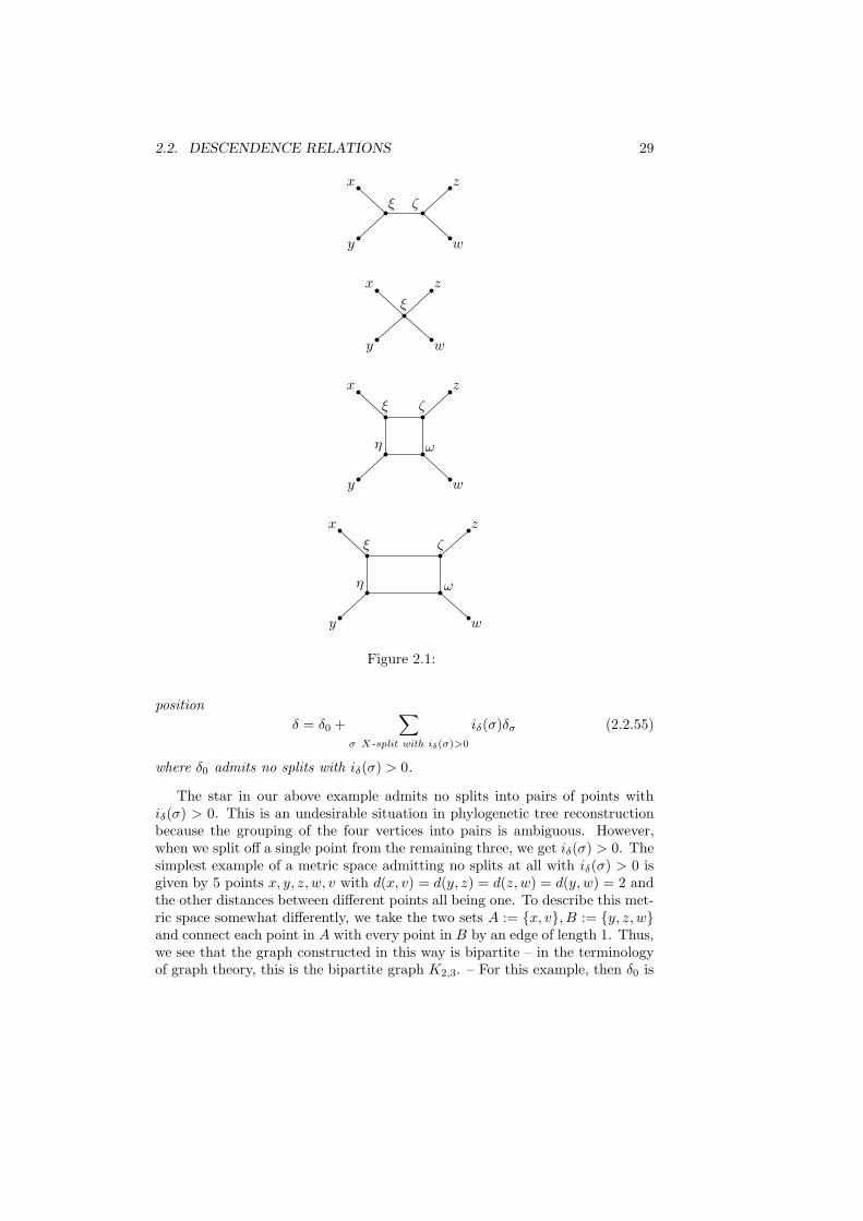
These examples will be graphically displayed in the figure below. We first takea space X = x, y, z, w consisting of 4 points, with the condition
δ(x, y) + δ(z, w) < max(δ(x, z) + δ(y, w), δ(x,w) + δ(y, z)). (2.2.53)
If δ(x, y) = δ(z, w) = 2, δ(x, z) = δ(x,w) = δ(y, z) = δ(y, w) = 3, the splitx, y|z, w has index iδ = 1/2 and is induced from a tree with leaves x, y, z, wand interior nodes ξ, ζ with δ(x, ξ) = δ(y, ξ) = δ(ξ, ζ) = δ(z, ζ) = δ(w, ζ) = 1.The splits x, z|y, w or x,w|y, z, however, have iδ(σ) = 0 and are notinduced by that tree metric. When we have equality in (2.2.53), say, δ(x, y) =δ(z, w) = 2, δ(x, z) = δ(z, w) = δ(y, z) = δ(y, w) = 2, the metric can still berepresented by a tree metric, this time with a single interior vertex ξ that hasdistance 1 from all leaves. We call this tree a star. Here, there is no longera natural grouping of the vertices into two pairs. – When instead δ(x, y) =δ(z, w) = δ(x, z) = δ(y, w) = 3, and δ(x,w) = δ(y, z) = 4, then (2.2.53) holdsagain. This time, we can represent the metric by a graph with 4 interior verticesξ, η, ζ, ω that is not a tree. ξ, η, ζ, ω form a rectangle with δ(ξ, η) = δ(ξ, ζ) =δ(ω, ζ) = δ(η, ω) = 1, the other nontrivial distances between them being equalto 2, and with x connected to ξ, y to η, z to ζ, w to ω, all with distance 1.Thus, we need to insert an interior rectangle in order to represent the metric ona graph. That rectangle then expresses the ambiguity in the dissimilarity mapfor a hierarchical grouping. Of course, the rectangle is in fact a square, andso there is some special symmetry. We therefore also consider the case whereδ(x, y) = δ(z, w) = 3, δ(x, z) = δ(y, w) = 4, δ(x,w) = δ(y, z) = 5. In thatcase, we again insert 4 interior vertices ξ, η, ζ, ω that form a rectangle, this timewith δ(ξ, η) = δ(η, ω) = 1, δ(ξ, ζ) = δ(ω, ζ) = 2. In any case, when we havesuch a rectangle, we produce splits by cutting pairs of parallel edges. Cuttingthe edges between ξ and ζ and between η and ω, for example, produces thesplit x, y|z, w. Cutting the edges between ξ and η and between ζ and ωinstead produces the split x, z|y, w. Now, in contrast to the tree case, boththese splits have iδ(σ) > 0. The split x,w|y, z, however, has iδ(σ) < 0.In the tree case, interchanging x with y or z with w would not have made anydifference for the distances between those 4 vertices, but this is no longer so inthe rectangle case.
After this example, let us return to the general case. When δ is a tree metricfrom an X-tree (T, φ), the split σ of X is induced by that X-tree precisely ifiδ(σ) > 0. In that case, we then have iδ(σ) = w(eσ) for the weight of the edgeinducing the split. And we can rewrite (2.2.51) then as
δ =∑
σ X-split with iδ(σ)>0
iδ(σ)δσ. (2.2.54)
The split decomposition theorem of Bandelt and Dress[1] then says that everydissimilarity map can be written as a sum over such tree metrics plus a remainderthat has no splits with iδ(σ) > 0:
Theorem 2.2.3. Let δ be any dissimilarity map on X. We then have a decom-
2.2. DESCENDENCE RELATIONS 29
ζξ
z
w
x
y
ξ
z
w
x
y
ζ
ω
ξ
η
z
w
x
y
ζ
ω
ξ
η
z
w
x
y
Figure 2.1:
position
δ = δ0 +∑
σ X-split with iδ(σ)>0
iδ(σ)δσ (2.2.55)
where δ0 admits no splits with iδ(σ) > 0.
The star in our above example admits no splits into pairs of points withiδ(σ) > 0. This is an undesirable situation in phylogenetic tree reconstructionbecause the grouping of the four vertices into pairs is ambiguous. However,when we split off a single point from the remaining three, we get iδ(σ) > 0. Thesimplest example of a metric space admitting no splits at all with iδ(σ) > 0 isgiven by 5 points x, y, z, w, v with d(x, v) = d(y, z) = d(z, w) = d(y, w) = 2 andthe other distances between different points all being one. To describe this met-ric space somewhat differently, we take the two sets A := x, v, B := y, z, wand connect each point in A with every point in B by an edge of length 1. Thus,we see that the graph constructed in this way is bipartite – in the terminologyof graph theory, this is the bipartite graph K2,3. – For this example, then δ0 is
30 CHAPTER 2. DISCRETE STRUCTURES
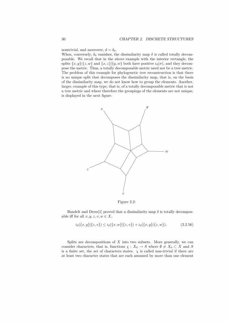
nontrivial, and moreover, d = δ0.When, conversely, δ0 vanishes, the dissimilarity map δ is called totally decom-posable. We recall that in the above example with the interior rectangle, thesplits x, y|z, w and x, z|y, w both have positive iδ(σ), and they decom-pose the metric. Thus, a totally decomposable metric need not be a tree metric.The problem of this example for phylogenetic tree reconstruction is that thereis no unique split that decomposes the dissimilarity map, that is, on the basisof the dissimilarity map, we do not know how to group the elements. Another,larger, example of this type, that is, of a totally decomposable metric that is nota tree metric and where therefore the groupings of the elements are not unique,is displayed in the next figure.
yx
z
v
w
Figure 2.2:
Bandelt and Dress[1] proved that a dissimilarity map δ is totally decompos-able iff for all x, y, z, v, w ∈ X ,
iδ(x, y|z, v) ≤ iδ(x,w|z, v) + iδ(x, y|z, w). (2.2.56)
Splits are decompositions of X into two subsets. More generally, we canconsider characters, that is, functions χ : X0 → S where ∅ 6= X0 ⊂ X and Sis a finite set, the set of characters states. χ is called non-trivial if there areat least two character states that are each assumed by more than one element
2.2. DESCENDENCE RELATIONS 31
of X0. We say that the character χ factors through the X-tree (T, φ) whenthere exists χ′ : T → S (here, we mean by a function on the tree T a functionthat is defined on the vertices of T ) with χ = χ′ φ|X0
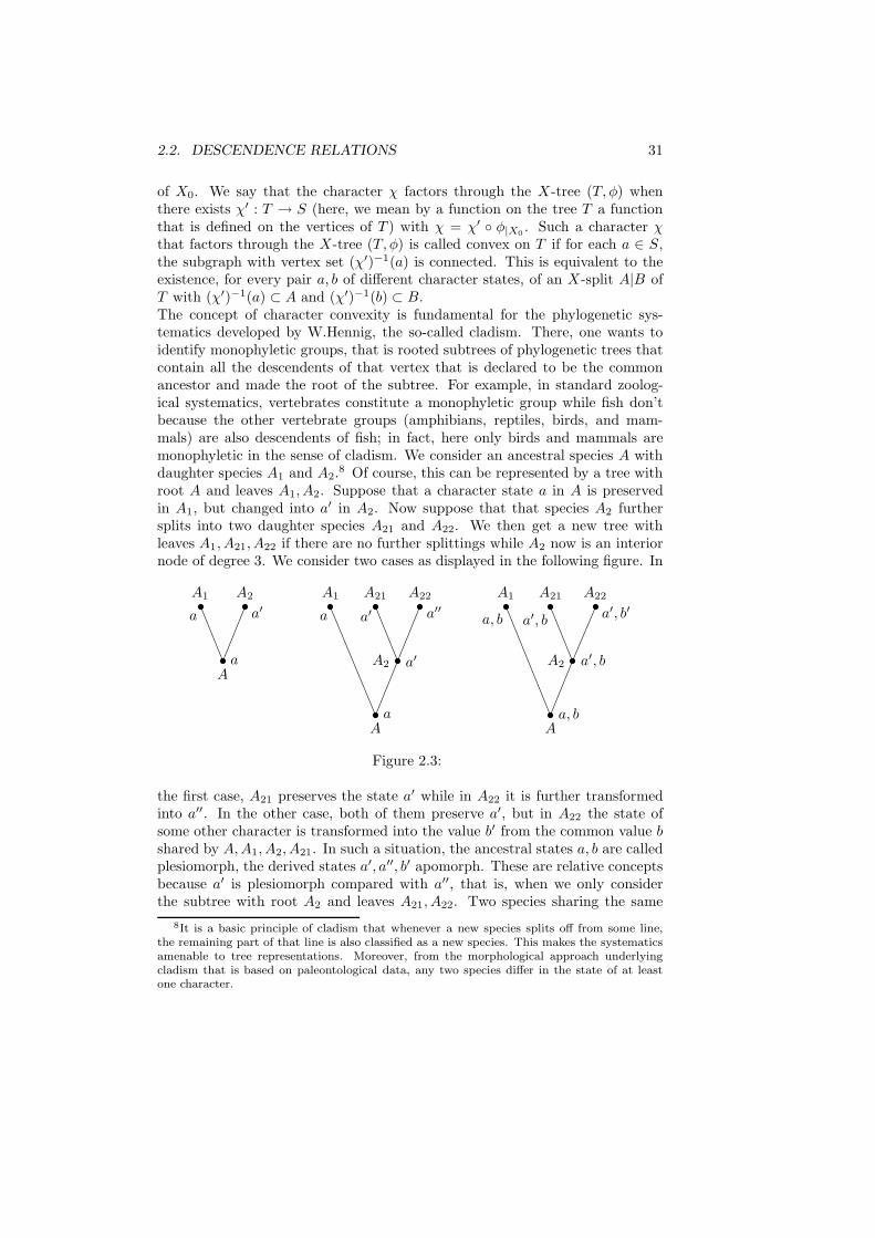
. Such a character χthat factors through the X-tree (T, φ) is called convex on T if for each a ∈ S,the subgraph with vertex set (χ′)−1(a) is connected. This is equivalent to theexistence, for every pair a, b of different character states, of an X-split A|B ofT with (χ′)−1(a) ⊂ A and (χ′)−1(b) ⊂ B.The concept of character convexity is fundamental for the phylogenetic sys-tematics developed by W.Hennig, the so-called cladism. There, one wants toidentify monophyletic groups, that is rooted subtrees of phylogenetic trees thatcontain all the descendents of that vertex that is declared to be the commonancestor and made the root of the subtree. For example, in standard zoolog-ical systematics, vertebrates constitute a monophyletic group while fish don’tbecause the other vertebrate groups (amphibians, reptiles, birds, and mam-mals) are also descendents of fish; in fact, here only birds and mammals aremonophyletic in the sense of cladism. We consider an ancestral species A withdaughter species A1 and A2.
8 Of course, this can be represented by a tree withroot A and leaves A1, A2. Suppose that a character state a in A is preservedin A1, but changed into a′ in A2. Now suppose that that species A2 furthersplits into two daughter species A21 and A22. We then get a new tree withleaves A1, A21, A22 if there are no further splittings while A2 now is an interiornode of degree 3. We consider two cases as displayed in the following figure. In
Aa
A2
a′A1
a
A2 a′
A22
a′′A21
a′
Aa
A1
a
A2 a′, b
A22
a′, b′A21
a′, b
Aa, b
A1
a, b
Figure 2.3:
the first case, A21 preserves the state a′ while in A22 it is further transformedinto a′′. In the other case, both of them preserve a′, but in A22 the state ofsome other character is transformed into the value b′ from the common value bshared by A,A1, A2, A21. In such a situation, the ancestral states a, b are calledplesiomorph, the derived states a′, a′′, b′ apomorph. These are relative conceptsbecause a′ is plesiomorph compared with a′′, that is, when we only considerthe subtree with root A2 and leaves A21, A22. Two species sharing the same
8It is a basic principle of cladism that whenever a new species splits off from some line,the remaining part of that line is also classified as a new species. This makes the systematicsamenable to tree representations. Moreover, from the morphological approach underlyingcladism that is based on paleontological data, any two species differ in the state of at leastone character.
32 CHAPTER 2. DISCRETE STRUCTURES
plesiomorph state of a character are called symplesiomorphic w.r.t. that char-acter, those sharing an apomorphic state are called synapomorphic. In the lastexample, A1 and A21 are symplesiomorphic for b while A21 and A22 are synapo-morphic w.r.t. a′. In the preceding example, where A22 had the character statea′′, the states a′, a′′ together constitute a synapomorphy between A21 and A22.Only synapomorphy, but not symplesiomorphy, can be an indication of a mono-phyletic group. Here then enters the convexity assumption. Namely, in order tobe able to use shared derived characters, that is, synapomorphies for identifyingmonophyletic groups, we must exclude the following two possibilities:
1. Reversion: In the last example, A22, instead of assuming the new statea′′, reverts to the ancestral state a.
2. Convergence: In the same example, A1, instead of keeping the state b,assumes the same state b′ that originated in the species A22 while A21
kept b.
Of course, there exist biological examples for either possibility. Snakes have lostthe limbs that their ancestors had gained. Birds, bats, and insects have inde-pendently developed wings. In fact, the wings of birds and bats are plesiomorphwhen considered as forelimbs, but not as wings. Sometimes, the distinction be-tween plesiomorphy and apomorphy is not clear or needs to be reconsidered inthe light of genetic sequence data. For example, it had been thought for a longtime that the eyes in arthropods, molluscs, and vertebrates are examples of aconvergent evolution. It has been discovered, however, that eye formation in allthese lineages is directed by the same type of controlling gene from the class ofhomeotic (Hox) genes. An uncontroversial9 example of convergence is mimikrywhere one species imitates the coloration or other pattern of an unrelated speciesthat is avoided by predators. In any case, reversion and convergence are rela-tively rare in biological evolution, however. Both these possibilities are excludedby character convexity.When one has several characters, one wants to find a single X-tree for whichall of them are convex. When such a tree exists, these characters are calledcompatible. As for compatibility of splits, there exists a theorem characterizingthe compatibility of characters, but since the formulation is more complicatedwe refer to [33].When working with biological data, typically not all the characters are compat-ible, and one then wishes to quantify that non-compatibility and construct atree that comes as close as possible to rendering all the characters convex. Thisis the idea of parsimony. More precisely, given a function f on the vertex setV of a graph Γ, the changing number of f is the number of those edges of Γon whose endpoints f assumes different values, that is, the number of all edgese = (i, j) with f(i) 6= f(j). Let now χ : X0 → S be a character that factors
9at least as long as one does not look at the underlying genetic mechanisms; in fact, it maywell turn out in a given example that the imitation of a pattern is produced by the same kindof genetic regulatory mechanism as the imitated pattern, and at least the general frameworkof that genetic regulation might be derived from some common ancestor
2.2. DESCENDENCE RELATIONS 33
through the X-tree (T, φ), with χ = χ′ φ|X0as above. Here, we are assuming
that χ′ is already defined on all the vertices of T . Of course, it is then arbitraryhow to define χ′ on those vertices of T that are not in the image of φ(X0), incase φ is not surjective on X0. For a character χ, we then define its parsimonyscore s(χ, T ) for the X-tree (T, φ) as the minimal changing number of all thoseextensions χ′ on T that factor χ. Given a set of characters, its parsimony scoreon an X-tree then is simply the sum of the individual parsimony scores. Amaximal parsimony X-tree for that set of characters then is one that minimizesthat parsimony score.It is not difficult to see that the parsimony score is related to character con-vexity. In fact, given a character that assumes ν different states, the so-calledhomeoplasy of the character χ on T
h(χ, T ) := s(χ, T )− ν + 1 ≥ 0 (2.2.57)
with equality precisely if χ is convex on T . Thus, the total homeoplasy of acharacter set, the sum of the individual homeoplasies, is also non-negative andvanishes precisely when the characters are compatible.The concept of maximum parsimony trees is not without difficulties, both con-ceptually and mathematically. The conceptual difficulties arise from the arbi-trariness in the definition and choice of characters. It is a fundamental problemin paleontology and morphology to clearly state what a character is and todecide which characters are independent of each other. Of course, large setsof dependent characters would bias the parsimony concept. The mathematicalproblems will be taken up below when we consider stochastic processes on treesand other graphs. We shall then see that any method of reconstructing a struc-ture from a data set depends on a model for the underlying process that createdthe data.
A standard problem is to amalgate phylogenetic relationships between subsetsof X as expressed in trees into an encompassing tree representing all of X . Ofcourse, the issue of compatibility will arise again. The smallest meaningful sub-sets here consist of 4 elements and are called quartets, and trees with 4 leaves arecalled quartet trees. Also, if one has data about the relationships between theelements of X and wants to construct a tree or, more generally, find out whetherthese relationships fit into a tree, a natural strategy is to first construct all localquartet trees and then assemble those into a common tree. When we have acollection Q of quartet trees that contains exactly one quartet tree a, b|c, dfor every quartet Y = a, b, c, d of X , then, as discovered by Colonius andSchulze [6], there exists a unique X-tree containing all these quartet tree iff thefollowing two quartet rules hold for all a, b, c, d, e ∈ X :
1.
If a, b|c, d, a, b|d, e ∈ Q, with c 6= e, then a, b|c, e ∈ Q
2.If a, b|c, d, a, c|d, e ∈ Q, then a, b|c, e ∈ Q.
34 CHAPTER 2. DISCRETE STRUCTURES
In practice, of course, these rules will be violated for some quintuples of elementsof X , and one therefore cannot construct a tree.There are other, in fact infinitely many, quartet rules. If Q does not contain aquartet tree for every quartet in X , that is, if we only have a subcollection ofquartet trees, then we need to invoke more of those rules to check for compati-bility, see [33] for more on this topic. For an algorithm for the (re)constructionof a tree from quartets, see [35].
2.2.2 Genealogies (pedigrees)
While species can be considered as important biological entities in their ownright, the ancestor-descendent relationships in phylogenetic trees can also beviewed as accumulated genealogies of the individuals constituting the popula-tions underlying the species. Thus, let us consider those genealogies a little,even though they in turn can be viewed as combinations of inheritance pro-cesses of genes passed on from parents to offspring. The latter, in fact, will leadus back to trees below.The genealogy or pedigree of an individual in a sexually recombining populationis a directed graph. Each individual has two incoming links from its parentswhile the number of outgoing links counts its offspring. Since no individual canbe a descendent of its own offspring, or an ancestor of its own parents, the graphis acyclic (it has no directed cycles; the underlying undirected graph may wellhave cycles as the result of inbreeding in the population). The nodes withoutoutgoing links represent those individuals that did not produce or have not yetproduced offspring. When the graph represents a population history, one can es-sentialize it by pruning all the vertices without outgoing links that correspondsto individuals no longer alive. This will then be an iterative process because inthe next step one would have to prune those vertices that have outgoing linksonly to vertices that have been pruned in the previous step. In that manner,one iteratively eliminates all vertices that do not have living descendents. Thus,one is left with the ancestral relationships leading to the present population.Since one does not want to extend the pedigree to the infinite past, one startswith some ancestral population. The essentialized pedigree then contains onlythose members of the ancestral population that have descendents in the presentgeneration. If one moves further to the next generation, then some of those an-cestors may cease to have descendents and therefore will get eliminated. Someof those ancestors, called the lucky ones, however, will turn out to be ancestorsof all members of the present population, and they will therefore also leave de-scendents in all future generations, until the entire population goes extinct.Often, one assumes that the different generations do not overlap. The genera-tions can then be labelled by their distance from the ancestral one, and linksalways go from generation n to generation n+ 1.Also, from the pedigree graph, one can construct another graph expressingmating relationships. In that graph, there is an (undirected) edge between twoindividuals when they have produced offspring together. When the species isdioeceous, that is, has separate sexes, the mating graph is bipartite, the two
2.2. DESCENDENCE RELATIONS 35
classes corresponding to the females and the males. The mating graph usuallyis not connected, however, therefore, strictly speaking, violating our definitionof a graph. When the population is strictly monogamous, the graph consists ofdisjoint pairs only, after we have essentialized it and eliminated all the bachelorsand spinsters.Of course, this is all rather simple. Later on, when we consider stochas-tic branching processes, pedigrees of sexually recombining populations becomerather difficult, but for the moment we leave the subject and turn to
2.2.3 Gene genealogies (coalescents)
The pedigree just considered for a dioeceous population contains two trees (moreprecisely, so called forests, that is, not necessarily connected unions of trees) assubgraphs, namely the ones corresponding to the male and the female individ-uals. Let us take one of them, say the female one. Thus, we only considermother-daughter relationships. For two individuals, we can then ask when theirlineages coalesce or merge back in the past, that is, how many generations backthey had the same female ancestor. For two sisters, we need only go one genera-tion back, as they have the same mother, while first (in the female line) cousinsshare a maternal grandmother, and so on. Once the lineages coalesce, they willstay together all the way back to the ancestral population. Of course, in prin-ciple, they may never merge, that is the two females under consideration maybe descendents of different females in the ancestral population. When we gosufficiently many generations back into the past, however, with overwhelmingprobability, all presently living females in the populations will descend from thesame ancestral female, the “Eve”. All other females in that ancestral populationwill then have no descendents from an uninterrupted female line in the presentpopulations; of course they may or may not have descendents from some lin-eages that include some males. As already described above, we can essentializethe graph by eliminating all females without female descendents in an iterativemanner so that only those remain that have an uninterrupted line of femaledescendents down to the present sample. When we do coalescence theory, thatis, follow the ancestry of the present sample back in time, then, in fact, thoseeliminated individuals will never occur in the consideration. This representsan enormous simplification in practice when compared with considering the for-ward branching process for the (female) descendents of an ancestral populationswhere all descendents will occur regardless of whether they contribute to futuregenerations or not.
Let us consider this scenario in more detail in a simple example that will leadus to the Wright-Fisher model of population genetics. We consider a populationwith non-overlapping generations, and we assume that the size of the popula-tion remains constant = 2N across generations. We also assume, for simplicity,that the sex ratio remains constant and equal so that we are dealing with apopulation of N females. The assumption of the Wright-Fisher model is that,given generation n, consisting of a population of N individuals, generation n+1
36 CHAPTER 2. DISCRETE STRUCTURES
is (mathematically) created by choosing N times randomly and independentlyan individual from generation n as mother. Here, it is assumed that the popu-lation is entirely homogeneous, or, in more biological terms, that all membersare equally fit, so that at each selection step, each member has the same chanceof being chosen. Also, creating daughters does not affect the fitness, and so,the chance to be chosen at a given step does not depend on how often one hasalready been chosen in previous steps. Putting it another way, each individualin generation n+ 1 picks individual j in generation n with probability 1/N asits mother, and this sampling is carried out N times with replacement. If djis the number of daughters of individual j, we thus have for the probability ofhaving ν daughters
p(dj = ν) =
(
N
ν
)
(1
N)ν(1 − 1
N)N−ν . (2.2.58)
This is a binomial distribution, Bi(N, 1N ), and so, the number of daughters of
a given female is binomially distributed. The expectation value is
E(dj) = N1
N= 1 (2.2.59)
which of course reflects the fact that the population size is constant, and thevariance is
V ar(dj) = N1
N(1 − 1
N) = 1 − 1
N(2.2.60)
(see (3.1.20) below). The correlation between the numbers of daughters ofdifferent females j, k is
Cor(dj , dk) =Cov(dj , dk)
√
V ar(dj)V ar(dk)= − 1
N − 1. (2.2.61)
The correlation is negative, again because the population size is constant, andtherefore, when j has many daughters, there is less room for k to have manydaughters as well (when we already know that an individual different from j hasone daughter, then the expected number of daughters of j is reduced to N−1
N inplace of the value 1 of (2.2.59)). This effect is rather small in large populations.For large N , the binomial distribution Bi(N, 1
N ) is approximated by a Poissondistribution
p(dj = ν) ≈ 1
ν!e−1 (2.2.62)
with mean and variance =1 (see (3.1.8), (3.1.9) in 3.1 below). In particular, theprobability of having no daughters is
p(dj = 0) ≈ e−1 ≈ .37 (2.2.63)
while then the probability to have at least one daughter becomes
p(dj > 0) ≈ 1 − e−1 ≈ .63 (2.2.64)
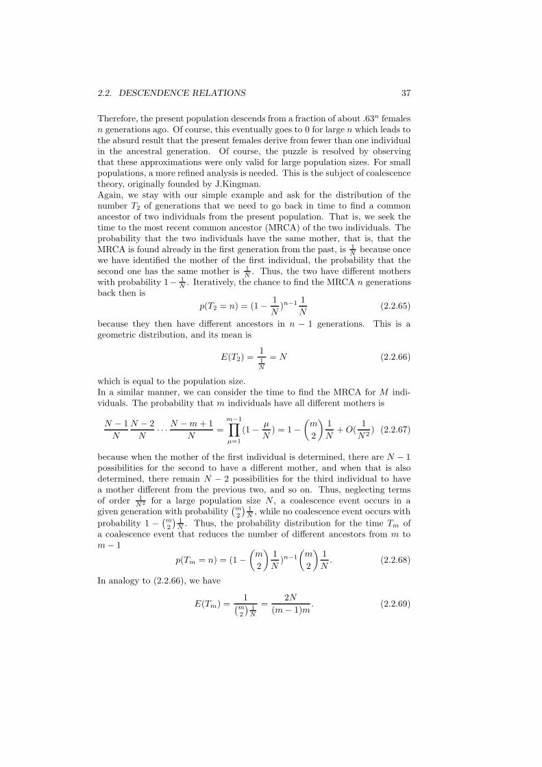
2.2. DESCENDENCE RELATIONS 37
Therefore, the present population descends from a fraction of about .63n femalesn generations ago. Of course, this eventually goes to 0 for large n which leads tothe absurd result that the present females derive from fewer than one individualin the ancestral generation. Of course, the puzzle is resolved by observingthat these approximations were only valid for large population sizes. For smallpopulations, a more refined analysis is needed. This is the subject of coalescencetheory, originally founded by J.Kingman.Again, we stay with our simple example and ask for the distribution of thenumber T2 of generations that we need to go back in time to find a commonancestor of two individuals from the present population. That is, we seek thetime to the most recent common ancestor (MRCA) of the two individuals. Theprobability that the two individuals have the same mother, that is, that theMRCA is found already in the first generation from the past, is 1
N because oncewe have identified the mother of the first individual, the probability that thesecond one has the same mother is 1
N . Thus, the two have different motherswith probability 1− 1
N . Iteratively, the chance to find the MRCA n generationsback then is
p(T2 = n) = (1 − 1
N)n−1 1
N(2.2.65)
because they then have different ancestors in n − 1 generations. This is ageometric distribution, and its mean is
E(T2) =11N
= N (2.2.66)
which is equal to the population size.In a similar manner, we can consider the time to find the MRCA for M indi-viduals. The probability that m individuals have all different mothers is
N − 1
N
N − 2
N· · · N −m+ 1
N=
m−1∏
µ=1
(1 − µ
N) = 1 −
(
m
2
)
1
N+O(
1
N2) (2.2.67)
because when the mother of the first individual is determined, there are N − 1possibilities for the second to have a different mother, and when that is alsodetermined, there remain N − 2 possibilities for the third individual to havea mother different from the previous two, and so on. Thus, neglecting termsof order 1
N2 for a large population size N , a coalescence event occurs in agiven generation with probability
(
m2
)
1N , while no coalescence event occurs with
probability 1 −(
m2
)
1N . Thus, the probability distribution for the time Tm of
a coalescence event that reduces the number of different ancestors from m tom− 1
p(Tm = n) = (1 −(
m
2
)
1
N)n−1
(
m
2
)
1
N. (2.2.68)
In analogy to (2.2.66), we have
E(Tm) =1
(
m2
)
1N
=2N
(m− 1)m. (2.2.69)
38 CHAPTER 2. DISCRETE STRUCTURES
When we then want to go back from M individuals to a single ancestor, we needto consider all the coalescent events from m to m− 1 for m = 2, . . . ,M . Sincethe times for these events are independent of each other, the expected numberof generations back in the past for M female individuals to have a single femaleancestor is
M∑
m=2
E(Tm) =
M∑
m=2
1(
m2
)
1N
=
M∑
m=2
2N
(m− 1)m= 2N(1 − 1
M). (2.2.70)
In other words, this is the expected height (measured in number of generations)of the tree starting with a single female ancestor and leading to the presentensemble of M females. When we compare (2.2.70) with (2.2.66), we see thatthe latter is less than 2 times the former. This means that the final step ofreducing the number of ancestors from 2 to 1 typically takes at least half thetime of the whole process. Thus, the long branches of the tree arise when thereare only few females in the ancestry of the sample.One can, of course, perform the same analysis with males in place of females. Letus insert a small variation, however, to account for the fact that in many animalspecies, like most mammals, and also in many human societies, the variance inthe number of offspring for males is considerably higher than for females whileobviously the expectation value is the same, assuming that the population is ingender equilibrium. This higher variance is easy to achieve in our model. Thesimplest version just stipulates that in each generation only a certain fraction0 < q < 1 of the number of males is having offspring at all. When we then lookfor the father of an individual, each of those ones is taken with probability 1/qNwhile the other ones are simply discarded. Thus, two individuals now stand achance of 1/qN of having the same father. Thus, N gets replaced by qN in allformulae. In particular, the expectation values for the waiting times in (2.2.66),(2.2.70) are shortened by a factor q, and we expect to find the MRCA in themale line correspondingly fewer generations ago than the one in the female line.In other words, “Adam” lived many generations after “Eve”.
Coalescence theory is mainly interested in describing the ancestry of genes,or more precisely, of DNA segments, rather than of individuals. Formally, thebasic scenario is the same, however, and therefore, we have described the basicsituation above for the more intuitive case of individuals. The basic scenarioneglects the issues of mutation and recombination. In order to exclude recom-bination, there are two possibilities, one of significance for biological data, theseother one solely for modeling purposes. The first one consists in consideringthose DNA segments that do not recombine. One class is given by non-nuclearmitochondrial DNA that is only contained in egg cells, but not in sperm, andtherefore is only passed on in the female line. This, in fact, makes the aboveexample of female lineages relevant for treating biological data. The other ex-ample is the Y-chromosome in humans and other mammals which is only carriedby males (and determines the male gender) and therefore is only transmittedin the male lineage. The mathematically convenient solution, in contrast, is to
2.2. DESCENDENCE RELATIONS 39
simply consider the smallest DNA segments, the single nucleotides.The biolog-ical problem here is that even though each nucleotide is derived from a uniqueparent, this usually cannot be identified from genetic data because in a givenspecies,at most positions, most members share the same nucleotide. Neverthe-less, for so-called SNPs, single nucleotide polymorphisms, consideration of singlenucleotide positions can contain some useful population biological information.Even when we consider single nucleotide positions, however, we only get rid ofthe problem of recombination while absence of mutations, and of other processesof genetic rearrangement, then is still a hypothesis imposed. For simplicity ofthe model, we also consider the haploid case where each individual has only oneset of genes. Thus, each such DNA segment in an individual is derived fromone of the parents. (In the diploid case, each individual has two sets of genes.The genes corresponding to each other in those sets are selected from differentparents, that is, one is taken from the mother and the complementary one fromthe father. This imposes additional restrictions when compared with the hap-loid case, but typically their effect is not so prominent.) For single nucleotidesin the haploid case which we shall now consider the situation is formally thesame as that one of the two parents of each individual is its mother. So, onemight call that individual that gives the nucleotide in question the nucleotideparent for that particular position in the DNA. When in turn we consider onlynucleotide parents, for a fixed position, then the situation is the same as before,with the only formal difference that two siblings can derive the nucleotide atthat position from different parents. Therefore, the size of the population thathas to be taken into account is 2N in place of N .In any case, for each such nucleotide position, we can perform the coalescentanalysis and find the expected number of generations for having a single an-cestor. Of course, the ancestors for the different positions will in general bedifferent individuals. We can then also ask the following questions
1. What is the expected number of generations for finding a single ancestorfor each position? That is, what is the expected maximal height of thecoalescence trees for a given population?
2. In the corresponding ancestral population, how many individuals are an-cestors for some position for the present sample? Those lucky ancestorsthen are ancestors of every individuum in the present sample whereas theremaining members of the ancestral population then are not geneticallyrepresented at all in that present sample because for each position, thereis only one ancestor by assumption.
3. Actually, the last issue is a little more subtle. In principle, an individuumin the ancestral population can be a genealogical ancestor of a presentone without being genetically represented in the latter. What are thechances for that? Here, one should essentially use some tree countingarguments. The pedigree graph contains many trees with a root in theancestral population and leading down to the present population, and each

40 CHAPTER 2. DISCRETE STRUCTURES
such root then represents a genealogical ancestor. Not all of these trees,however, arise from the coalescence processes just investigated.
So far, only some partial answers are known to these questions, see [17] for abrief discussion and references.
Chapter 3
Stochastic processes
3.1 Random variables
A general reference for this chapter is [15].Let (Ω,Σ, p) be a measure space, that is, a set Ω with a probability measure pand a Sigma algebra Σ of measurable sets. A measurable function
X : Ω → R (3.1.1)
then is called a random variable. The possible values of X are called events.Thus, what is random here is not the function X , but rather its argument ω ∈ Ωthat is considered to be drawn according to the measure p. The elements of Ωmay represent the possible outcomes of some experiment or observation. Whentossing a coin, for example, there are two possible outcomes, heads H and tailsT , and these then are the elements of Ω. When the coin is tossed twice, theappropriate Ω contains 4 elements, HH,HT, TH, TT . The random variablemay be the number of heads; in the last example, it may take the values 0,1,and 2. In this situation, X takes only discrete values, and whenever that isthe case, we speak of a discrete random variable. When it takes its values inthe non-negative integers N = 0, 1, 2, . . ., we have a counting variable. Thiswill be the important case for us. For a discrete random variable, we have the(probability) mass function
p(x) := p(X = x) := p(ω ∈ Ω : X(ω) = x), (3.1.2)
with some abuse of notation (more precisely, we are using the symbol p bothfor the probability measure in Ω and for the probability measure in R inducedby X – when there is a danger of confusion, we shall write pX for the latter).The distribution function of the random variable X is the function f(x) :=p(X ≤ x).When Y : Ω → R is another random variable, we can consider the joint massfunction
p(x, y) := p(X = x, Y = y) := p(ω ∈ Ω : X(ω) = x, Y (ω) = y) (3.1.3)
41
42 CHAPTER 3. STOCHASTIC PROCESSES
and the conditional one,
p(y|x) := p(Y = y|X = x) =p(X = x, Y = y)
p(X = x)(3.1.4)
whenever p(X = x) > 0, which satisfies
p(Y = y) =∑
x
p(Y = y|X = x)p(X = x) =∑
x
p(X = x, Y = y). (3.1.5)
The random variables X and Y are called independent if the probabilities forall events x of X and y of Y satisfy
p(X = x, Y = y) = p(X = x)p(Y = y). (3.1.6)
X and Y are called identically distributed if for every z ∈ R
p(X = z) = p(Y = z). (3.1.7)
The abbreviation “i.i.d” meaning independent and identically distributed is fre-quently used.In the above example, we may take X as the number of heads. When the coinis fair, that is, when HH,HT, TH, TT each occur with probability 1/4, we havep(0) = 1/4, p(1) = 1/2, p(2) = 1/4. More generally, when heads turn up withprobability q, and if the results of the two tosses are independent of each other,we have p(0) = (1 − q)2, p(1) = 2q(1 − q), p(2) = q2. More generally, if we tossthe coin n times, then
(
nk
)
points in the corresponding Ω, the set of the possibletossing sequences, yield k heads, and the mass function is
p(k) =
(
n
k
)
qk(1 − q)n−k. (3.1.8)
This is the binomial distribution Bi(n, q). When we let n → ∞, q → 0 in
such a manner that nq → λ 6= 0, then, using the approximations(
nk
)
≈ nk
k! and
(1 − q)n−k ≈ (1 − q)n = (1 − λn )n ≈ e−λ, we obtain the limit
(
n
k
)
qk(1 − q)n−k → λk
k!e−λ. (3.1.9)
This is the Poisson distribution Q(λ).The basic continuous distribution is the Gaussian distribution
1√2πσ
exp
(
− (x− µ)2
2σ2
)
(3.1.10)
on R with mean µ and variance σ2. Similarly, on Rn, we have the multinomial
Gaussian distribution1√2πσ
exp
(
−‖x− µ‖2
2σ2
)
, (3.1.11)
where ‖.‖ denotes the Euclidean norm, and x, µ ∈ Rn.
3.1. RANDOM VARIABLES 43
Definition 3.1.1. The k-th moment of the discrete random variable X withmass function p is the expectation value of Xk,
E(Xk) =∑
x
xkp(x). (3.1.12)
whenever that sum converges absolutely.
In fact, in order to make this consistent, one verifies more generally that forφ : R → R
E(φ(X)) =∑
x
φ(x)p(x) (3.1.13)
whenever the sum converges absolutely.When the random variable X is not discrete, the above sums get replaced byan integral; for example
E(Xk) =
∫
x
xkp(x)dx. (3.1.14)
For the moment, however, we consider discrete random variables.The first moment E(X) is of course the mean, average, or expectation valueof X , and the second moment then yields its variance var(X) = E(X2) −(E(X))2 = E((X − E(X))2).
We can also consider conditional expectations and obtain the following lemma
Lemma 3.1.1. Let X and Y be discrete random variables on Ω. The condi-tional expectation E(Y |X) =: φ(X) satisfies
E(φ(X)) = E(Y ). (3.1.15)
Proof. By (3.1.13) and (3.1.5)
E(φ(X)) =∑
x
φ(x)pX(x) =∑
x
∑
y
y pY |X(y|x)pX(x)
=∑
x,y
y pY (y) = E(Y ).
The random variables X and Y are called uncorrelated if
E(XY ) = E(X)E(Y ). (3.1.16)
Independent random variables are uncorrelated, but not necessarily conversely.The next result is easy:
44 CHAPTER 3. STOCHASTIC PROCESSES
Lemma 3.1.2. For random variables X,Y and α, β ∈ R, we havea)
E(αX + βY ) = αE(X) + βE(Y ). (3.1.17)
b)var(αX) = α2var(X) (3.1.18)
c) when X and Y are uncorrelated
var(X + Y ) = var(X) + var(Y ). (3.1.19)
a) simply expresses the linearity of the expectation value. Therefore, one mayperform arbitrary linear operations with random variables without requiringthat they be independent and have the corresponding operations on the expec-tation values.We apply this lemma to the binomial distribution Bi(n, q) from (3.1.8), in-terpreted as n independent tossings of a coin. Since the value of the ran-dom variable H , the number of heads, in a single toss is 0 or 1, we haveE(H2) = E(H) = q and so the variance E(H2)− (E(H))2 is q(1−q). Thus, therandom variable for the event H has expectation value q and variance q(1− q).We therefore obtain from the lemma
E(Bi(n, q)) = nq, var(Bi(n, q)) = nq(1 − q). (3.1.20)
For the Poisson distribution Q(λ) (3.1.9) obtained above as a limit of binomialdistributions, we obtain
E(Q(λ)) = var(Q(λ)) = λ. (3.1.21)
There are various notions of convergence for a sequence (Xn)n∈N of randomvariables towards a random variable X . Xn converges to X almost surely ifp(ω ∈ Ω : limn→∞Xn(ω) = X(ω)) = 1. It converges to X in kth mean (k ≥ 1)if all E(|Xn|k) < ∞ and limE(|Xn −X |k) = 0. The cases of most interest arek = 1 and k = 2. For k = 2, one speaks of convergence in mean square. (Xn)converges to X in probability if for all ε > 0, limn→∞ p(|Xn −X | > ε) = 0 (asusual, the expression here is shorthand for p(ω ∈ Ω : |Xn(ω) −X(ω)| > ε)).It converges to X in distribution if limn→∞ p(Xn ≤ x) = p(X ≤ x) for allx ∈ R for which the right hand side is continuous. Almost sure convergence andconvergence in kth mean (k ≥ 1) each imply convergence in probability, and thelatter in turn implies convergence in distribution, and convergence in kth meanimplies convergence in lth mean for k > l ≥ 1. There exist no other generalimplications between these notions of convergence.We now state some fundamental convergence theorems, referring to [15] forproofs. The first is the law of large numbers:
Theorem 3.1.1. Let Xn, n ∈ N be i.i.d random variables with E(|X1|) < ∞.With µ := E(X1), we then have
1
n
n∑
ν=1
Xν → µ almost surely. (3.1.22)

3.1. RANDOM VARIABLES 45
If E(X21 ) <∞, the convergence takes also place in mean square.
The next is the central limit theorem:
Theorem 3.1.2. Let (Xn) be a sequence of i.i.d. random variables with finitemean µ and finite variance σ2 6= 0. Then, for Sn :=
∑nν=1Xν , the distribution
of
Sn − nµ√nσ2
converges to the Gaussian distribution1√2π
exp(−x2
2). (3.1.23)
Let nowX : Ω → N (3.1.24)
be a discrete random variable that assumes only non-negative integer values.
Definition 3.1.2. The generating function of the random variable X is
G(s) := E(sX) =
∞∑
n=0
snp(n) (3.1.25)
(defined for those values of s ∈ R for which the sum converges).
Of course, the sequence p(n) can be recovered from the generating functionby evaluating its kth derivative at 0:
G(k)(0) = k! p(k) (3.1.26)
As we shall now see, the derivatives of G at 1 also encode important properties ofthe sequence p(n), namely its moments. Thus, when letting the argument s varyfrom 0 to 1, the generating function interpolates between the individual proba-bilities and collective properties of the distribution, the moments. Moreover, thegenerating function behaves in a very useful manner under composition of ran-dom processes and allows for a computation of moments of composed processesfrom the moments of the individual processes.
Lemma 3.1.3. a) Let G be the generating function of X. Then
E(X) = G′(1) and more generally E(X(X − 1) · · · (X − k + 1)) = G(k)(1)(3.1.27)
whenever that k-th derivative of G at s = 1 exists. (Thus, the moments of Xcan be computed recursively from the generating function.)b) If X1, . . . , XN are independent random variables, their generating functionssatisfy
GP
Nν=1Xν
(s) = GX1(s) · · ·GXN
(s). (3.1.28)
c) If X1, X2, . . . are independent and identically distributed random variableswhich then have the same generating function, denoted by GX , and if N : Ω → N
is another random variable independent of the Xν with generating function GN ,then the random variable Y = X1 +X2 + . . .XN (that is, the number of randomvariables occuring in the sum is now a random variable itself) has the generatingfunction
GY (s) = GN (GX(s)). (3.1.29)
46 CHAPTER 3. STOCHASTIC PROCESSES
Proof. a) is obvious, and b) follows from (3.1.16) applied to the independentrandom variables sXν . For c), from Lemma 3.1.1
GY (s) = E(sY ) = E(E(sY |N)) =∑
n
E(sY |N = n) pN (n)
=∑
n
E(s(X1+···+Xn)) pN(n)
=∑
n
E(sX1 ) · · ·E(sXn) pN (n) by b)
=∑
n
GX(s)n pN (n) = GN (GX(s)).
An alternative to the above polynomial generating function is the exponen-tial one where we replace s in (3.1.25) by et to get
H(t) := E(etX) =∞∑
n=0
entp(n). (3.1.30)
Here, the moments of p can directly be computed from the derivatives of H(t)at t = 1. All the formal results that we demonstrate about G also hold for H .In fact, for most purposes, the generating function H is more convenient thanG. In Theorem 3.4.1 below, however, we shall need a particular property of G,and this is the main reason why are working here systematically with G in placeof H . Also, it will be useful in our discussion of random graphs below.A variant of H is the discrete Fourier transform, the so-called characteristicfunction
E(eitX) =∞∑
n=0
eintp(n) =∑
n
∞∑
ν=0
(it)ν
ν!nνp(n), (3.1.31)
also called the moment generating function, that similarly encodes the proper-ties of the distribution p(n).
3.2 Random processes
Definition 3.2.1. A random or stochastic process is a family X = (Xt) ofrandom variables indexed by some set T ⊂ R.
Remark. More generally, one can allow for the Xt to take values in some mea-surable space other than R.
As Xt is a random variable, for each t, we get an induced probability distri-bution for the values of X by
pt(S) := p(Xt ∈ S) := p(ω ∈ Ω : Xt(ω) ∈ S) for a measurable S ⊂ R,(3.2.32)
3.3. POISSON PROCESSES AND NEURAL CODING 47
analogously to (3.1.2) (where we had only considered the case of discrete values).The random variables Xt1 and Xt2 (say t1 < t2) are independent, see (3.1.6), iffor S1, S2 ⊂ R
p(Xt1 ∈ S1, Xt2 ∈ S2) = p(Xt1 ∈ S1) p(Xt2 ∈ S2). (3.2.33)
The process is called stationary if its finite dimensional distributions are timeinvariant, i.e.
p(Xt1+τ ∈ S1, ..., Xtn+τ ∈ Sn) = p(Xt1 ∈ S1, ..., Xtn ∈ Sn) (3.2.34)
for all t1 < ... < tn, S1, ..., Sn ⊂ R and −∞ < τ <∞.
We shall now consider the case T = N.
Definition 3.2.2. The random process X is called a Markov chain if
p(Xn+1 = x|X1 = x1, X2 = x2, . . . , Xn = xn) = p(Xn+1 = x|Xn = xn)(3.2.35)
for all n ≥ 1, x, x1, . . . , xn ∈ R.
Definition 3.2.3. The random processX is called a martingale if E(|Xn|) <∞for all n and
E(Xn+1|X1, X2, ..., Xn) = Xn. (3.2.36)
We have the fundamental martingale convergence theorem
Theorem 3.2.1. A martingale X with E(X2n) < K < ∞ for some K and all
n converges to some random variable Ξ almost surely and in mean square.
3.3 Poisson processes and neural coding
In neurobiology, one studies spikes, that is, firings of neurons. Whereas thereexist biophysical models for the generation of spikes on the basis of the electro-chemical dynamics within neurons, see the Hodgkin-Huxley model described in4.3.1 below, in more abstract models of information processing, spikes are con-ceptualized as discrete events occurring at time points, that is, events withouttemporal duration. This motivates
Definition 3.3.1. A stochastic process (Nt)t∈T is called a point process whenT is an interval in R and the random variables Nt take only discrete values. Itis called a counting process when N0(ω) = 0 and Nt(ω) counts the number ofspecified events in the interval [0, t].
Of course, these concepts also apply to events other than spikes.Obviously, one can relax the normalizations, e.g., take some other t0 in place of0, without much gain of generality.
48 CHAPTER 3. STOCHASTIC PROCESSES
Since the realization ω ∈ Ω will not play a significant role in the sequel, we shallomit it in our notation and henceforth write
N(t) in place of Nt(ω).
One may also consider the probability distribution of the time interval betweenevents. The combination of these two points of view, that is, counting the num-ber of events having occured until time t vs. recording the temporal distancebetween subsequent events, will prove quite insightful. – If these time inter-vals are independently and identically distributed (a point to be returned toshortly), the process is called a renewal process. That is, the nth event occursat time t1 + t2 + ...tn where t1, ..., tn are independent positive random variablesthat are identically distributed according to some probability density functionp(t). When this distribution does not depend on time, the process is calledhomogeneous, else inhomogeneous.We return to the counting process.
Definition 3.3.2. A counting process N(t) is called locally continuous in prob-ability if
limǫց0
p(N(t+ ǫ) −N(t) ≥ 1) = 0. (3.3.37)
Definition 3.3.3. A counting process N(t) is said to have independent incre-ments if the numbers of events in disjoint time intervals are independent.
Definition 3.3.4. A counting processN(t) is said to have stationary incrementsif the number of events in a time interval depends only on the length of thattime interval.
Definition 3.3.5. A counting process N(t) that is locally continuous in proba-bility and has independent and stationary increments is called a (homogeneous)Poisson process.
Theorem 3.3.1. For a Poisson process N(t)
p(N(s+ t) −N(s) = n) = e−rt(rt)n
n!(3.3.38)
for n = 0, 1, . . . , for some constant r ≥ 0.
Thus, the number of events produced by a Poisson process is distributedaccording to the Poisson distribution Q(rt), see (3.1.9). The parameter rt ofthat distribution thus is proportional to the length t of the time interval, andthe factor r is called the rate of the process.
Proof. We put
ρ(t) := p(N(t) −N(0) ≥ 1) = p(N(s+ t) −N(s) ≥ 1) (3.3.39)
where the last equality holds because N has stationary increments. We claimthat
ρ(t) = 1 − e−rt (3.3.40)
3.3. POISSON PROCESSES AND NEURAL CODING 49
for some constant r ≥ 0. To see this, we start by observing that, by theassumption of independent increments, the probability π0(t + s) that no eventoccurs between 0 and t+ s equals the product of the probabilities that no eventoccurs in [0, t] and that no event occurs in [t, t + s]. By the assumption ofstationary increments, the latter equals the probability that no event occurs in[0, s], and hence
π0(t+ s) = π0(t)π0(s) (3.3.41)
whence π0(t) = π0(0) exp(−rt) for some constant r. r ≥ 0 since this probabilityis decreasing in t. Since π0(0) = 1 as N(0) = 0, we obtain
π0(t) = e−rt. (3.3.42)
Since this is the probability that no event occurs until t, the probability ρ(t)that the first event occurs before t is 1 − e−rt which is (3.3.40).Then
ρ(t) = rt+ o(t) for t→ 0. (3.3.43)
Similarly, the probability π1(t) := p(N(t) = 1) that precisely one event occursbetween 0 and t+ s satisfies
π1(t+ s) = π0(t)π1(s) + π1(t)π0(s) = e−rtπ1(s) + e−rsπ1(t). (3.3.44)
Using (3.3.43), we obtainπ1(t) = rte−rt. (3.3.45)
Iteratively, we obtain
πn(t) := p(N(t) = n) =(rt)n
n!e−rt. (3.3.46)
Recalling the assumption of stationary increments, this shows (3.3.38).
As a consistency check, the reader should verify that a counting processN(t) given by (3.3.38) with independent increments conversely has stationaryincrements and is locally continuous in probability.We also observe that
p(N(t) <∞) =∑
n≥0
p(N(t) = n) = e−rt∑
n≥0
(rt)n
n!= 1, (3.3.47)
and therefore, almost surely, only finitely many events take place in the finiteinterval [0, t]. Alternatively, this can also be directly be deduced from the as-sumptions. If there were infinitely many events in [0, t], then there would alsobe infinitely many events in either [0, t/2] or [t/2, t]. By the assumption of sta-tionary increments, then there would be infinitely many events in both theseintervals. Repeating this argument, there would be infinitely many events inevery subinterval of [0, t]. Consequently, every point would be an accumulationpoint of event, contradicting the assumption of local continuity in probability.

50 CHAPTER 3. STOCHASTIC PROCESSES
Theorem 3.3.2. For a Poisson process with rate r, the time of the nth eventis distributed according to
pn(t) =r(rt)n−1
(n− 1)!e−rt. (3.3.48)
Proof. We haved
dtp(N(t) = n) = pn(t) − pn+1(t), (3.3.49)
because the probability of having n events at time t goes up by the probabilitythat the nth event occurs at time t and goes down with the probability that the(n+1)st event occurs then. Since p0(t) = 0 for t > 0, (3.3.48) follows iterativelyfrom (3.3.46).
The argument of the proof can also be reversed: The probability of observingthe first event at t is given by the derivative of the probability for the first eventoccurring before t, that is, from (3.3.40), we obtain
p1(t) = re−rt, (3.3.50)
and as in the proof of Theorem 3.3.1, we can iterate that argument.We also have the consistency relation
n−1∑
ν=0
(rt)ν
ν!e−rt =
∫ ∞
t
r(rτ)n−1
(n− 1)!e−rτdτ (3.3.51)
(which follows from repeated integration by parts). The lhs is the probabilitythat at most n − 1 events have taken place up to time t (Theorem 3.3.1), andthe rhs that the nth event occurs after that time (Theorem 3.3.2).Assume that N(t) = n, that is, precisely n events occur in [0, t]. Since by theassumptions of stationary and independent increments, every n-tuple (t1, . . . , tn)of points in [0, t] has the same probability density of receiving those n events,that probability is given by
p(t1, ..., tn) =1
n!rne−rt (3.3.52)
because this depends on the length t of the interval and yields (3.3.38) byintegration w.r.t. t1, ..., tn from 0 to t. The combinatorial factor 1
n! arises,because the n events under consideration are indistinguishable. This also leadsto the correct normalization, because when we integrate w.r.t. t1, ..., tn andthen sum over all n, we obtain 1, by the relation
∑
n
1
n!(rT )n = erT . (3.3.53)
Theorem 3.3.3. Let N1(t), N2(t) be independent Poisson processes with ratesr1, r2. Then the counting process N(t) = N1(t) + N2(t) is a Poisson processwith rate r = r1 + r2.
3.3. POISSON PROCESSES AND NEURAL CODING 51
The proof is an obvious verification of the defining properties of a Poissonprocess.
Likewise, we can multiply the rate of a Poisson process with a constant positivefactor to obtain another Poisson process. In fact, when the factor is not con-stant, but is a function of time, we still obtain a process that is not significantlydifferent as we shall now explore.
Definition 3.3.6. Let r(t) be a continuous positive function on R+, and put
rt :=∫ t
0r(τ)dτ . A counting process N(t) with independent increments that
satisfies
p(N(s+ t) −N(s) = n) = e−rt(rt)
n
n!(3.3.54)
for n = 0, 1, . . . is called an (inhomogeneous) Poisson process with rate functionr(t).
Actually, this is not such a vast generalization (and we indicated that alreadyby the typographical similarity between rt and rt). Since the parametrizationof time is arbitrary, we have
Theorem 3.3.4. Any inhomogeneous Poisson process can be transformed intoa homogeneous one via a time reparametrization.
Proof. Since r(t) is assumed positive, rt is a strictly monotonically increasing,continuous function of t with r0 = 0 and limt→∞ rt = ∞. It therefore has aninverse function ρ(t) with the same properties. We put
N ′(t) := N(ρ(t)). (3.3.55)
This counting process then is a homogeneous Poisson process with rate 1 sincerρ(t) = t.
The assumption that r(t) be strictly positive could be relaxed to nonpositiv-ity. In that case, the time transformation would simply jump over those periodswhere r(t) vanishes.An equivalent characterisation of an inhomogeneous Poisson process with ratefunction r(t) is that it be a counting process with independent increments, sat-isfying
p(N(t+ǫ)−N(t) = 1) = r(ǫ)+o(ǫ) and p(N(t+ǫ)−N(t) ≥ 2) = o(ǫ) for ǫ→ 0.(3.3.56)
The first relation is a quantitative version of the local continuity in probability.The second relation automatically holds in the homogeneous case, but one needsto assume this in the inhomogeneous case.For an inhomogeneous Poisson process, the probability density for observingevents at the times t1, ..., tn is
p(t1, ..., tn) =1
n!exp(−
∫ t
0
r(τ)dτ)
n∏
i=1
r(ti). (3.3.57)
52 CHAPTER 3. STOCHASTIC PROCESSES
Using the time reparametrization of Theorem 3.3.4, this is deduced from theformula (3.3.52) for the homogeneous case. Upon integration, it yields (3.3.54),analogously to the homogeneous case.From (3.3.54), the expected number of events in the interval [0, t] is
∑
n
npt(n) =(rt)
n
(n− 1)!e−rt = rt =
∫ t
0
r(τ)dτ (3.3.58)
(see (3.3.53)).
Inhomogeneous Poisson processes are important models in theoretical neu-robiology (see e.g. [8]) because the rate r(t) that represents the spiking orfiring rate of a neuron can then depend on the stimulus S, that is, on the inputreceived by the neuron. Thus,
r(t) = r(t;S), (3.3.59)
and this represents the coding scheme of the neuron under consideration. Inother words, when receiving the stimulus S, the neuronal firing follows a Poissonprocess with rate r(t;S). For simplicity, we may assume that the stimulus isreceived at time t = 0. A basic model assumes that the neuron has a preferred oroptimal stimulus S0, and that the stimulus is translated via a Gaussian tuningfunction into the firing rate
r(t;S) = c exp
(
−d2(S, S0)
2σ2
)
. (3.3.60)
Here, d(., .) is some metric in the input space, for example a Euclidean one, thatis, d(S, S0) = ‖S − S0‖; c and σ2 (variance) are parameters. Obviously, othercoding schemes are possible.From (3.3.57), we see that the probability distribution for observing spikes pre-cisely at the times t1, ..., tn in the interval [0, t], given the input S is
p(t1, ..., tn|S) =1
n!exp
(
−∫ t
0
r(τ ;S)dτ
) n∏
i=1
r(ti;S). (3.3.61)
Bayes’ formula then yields the fundamental relationship for decoding the spiketrain produced by the neuron, that is, an estimate for the distribution of signalscontingent upon the recorded spike train t1, . . . , tn,
p(S|t1, ..., tn) = p(t1, ..., tn|S)p(S)
p(t1, ..., tn). (3.3.62)
Here, p(S) is a prior estimate for the distribution of stimuli (that may have beenobtained as the result of some learning process). p(t1, ..., tn) simply representssome normalization factor.
3.4. BRANCHING PROCESSES 53
Of course, (3.3.61) can also be used for other estimation schemes. For exam-ple, maximum likelihood selects a stimulus S that has caused an observed spikesequence with the highest probability, that is, S = argmax p(t1, ..., tn|S) in(3.3.61).
Clearly, a biological neuron does not operate according to a Poisson process.A spike is not an instantaneous event, but the generation of an action potentialhas a positive, although rather short, duration. Also, two spikes cannot be firedin too rapid succession because after a spike is fired, a neuron goes through arefractory periiod before it can generate the next spike. Thus, if one wants toinclude these aspects, one needs a biophysical in place of a purely phenomenolog-ical model. Such models exist, and we shall introduce and investigate below thebasic one, the Hodgkin-Huxley model. Notwithstanding its lack of biophysicalrealism, however, Poisson type models are very important in the neurosciencesbecause, on one hand, they relate well to the experimental practice of recordingspikes, and on the other hand, they can be the basis for models of informationtransmission in neural systems.
3.4 Branching processes
References for this section are [23, 16].We start with the simplest branching process, the Galton-Watson process. Here,each individual lives in a fixed generation n and independently of all otherindividuals produces a random number of offspring that become members ofgeneration n + 1. This random variable, the number of offspring, is the samefor all individuals in all generations. Thus, the numbers of offspring for theindividuals are independent and identically distributed random variables. Wedenote their common generating function by G(s). We also assume that thereis a positive probability for having more than one offspring. If the probabilityof having m offspring is p(m), this means that p(0) + p(1) < 1.Let the random variable Zn denote the size of generation n. One usually assumesthat the process starts with a single individual in generation 0, that is, Z0 = 1.Let Gn(s) = E(sZn) be the generating function of Zn.
Lemma 3.4.1. Gn is the n-th fold iterate of G,
Gn(s) = G · · · G(s), (3.4.63)
and thus also for m,n ∈ N
Gm+n(s) = Gm(Gn(s)). (3.4.64)
Proof. We shall show (3.4.64) which easily implies (3.4.63) by iteration. Let therandom variable Yi denote the number of members of the (m+ n)th generationthat derive from member i of the mth one. We then have
Zm+n = Y1 + · · · + YZm. (3.4.65)
54 CHAPTER 3. STOCHASTIC PROCESSES
By our assumptions, the Yi are independent and identically distributed, in factidentical to Zn, the number of offspring deriving from an individual n genera-tions ago. Lemma 3.1.3 c) then yields the claim.
Corollary 3.4.1. Let µ := E(Z1) and σ2 := var(Z1). Then
E(Zn) = µn and var(Zn) =
nσ2 if µ = 1σ2(µn−1)µn−1
µ−1 if µ 6= 1.(3.4.66)
Proof. Differentiating Gn(s) = G(Gn−1(s)) at s = 1 yields
E(Zn) = µE(Zn−1) (3.4.67)
from which the first equation follows by iteration. Differentiating twice givesG′′n(1) = G′′(1)G′
n−1(1)2 +G′(1)G′′n−1(1) which yields the second equation.
In view of this result, we call the process subcritical, critical, supercriticalwhen µ < 1,= 1, > 1, resp. In the sub- (super-)critical, we thus expect thepopulation to shrink (grow) while in the critical it is expected to stay the same.This might lead one to expect that the population will continue forever, butthat is not true as we shall now find out from asking whether the populationwill eventually become extinct, that is
Zn = 0 for some n ∈ N, and then of course also for all m ≥ n. (3.4.68)
Some observations are obvious:
• If p(0) = 0, that is, if every individual always has at least one offspring,then the population cannot become extinct. Therefore, we shall assumenow
p(0) > 0. (3.4.69)
• When p(ν) = 0 for ν ≥ 2, then p(0) + p(1) = 1. We have excludedp(0) = 0 and therefore cannot have the trivial case p(1) = 1, that is, thatevery individual has precisely one offspring so that the population size willalways remain constant. Consequently, the population should also becomeextinct because every individual then has either no or one offspring, andthe former with a positive probability. Therefore, the population willcertainly decrease. Therefore, we shall assume now
p(0) + p(1) < 1. (3.4.70)
Theorem 3.4.1. The extinction probability qextof the process, that is, the prob-ability that for some n ∈ N we have Zn = 0, equals the smallest root of theequation G(s) = s. For µ ≤ 1, we have qext = 1, that is, the population becomesextinct almost surely, while for µ > 1, we have qext < 1, that is, the populationhas a positive probability of surviving forever.
3.4. BRANCHING PROCESSES 55
Proof. We observe that G(s) as a power series with non-negative coefficientsp(ν) and p(0) + p(1) < 1 by our initial assumptions is increasing and strictlyconvex for s ∈ [0, 1] and satisfies G(0) = p(0), G(1) = 1. When µ = G′(1) ≤ 1,then G(s) > s for s ∈ [0, 1), while for µ > 1, G(s) = s has a unique root in[0, 1). These properties implies that G(s) = s has a smallest root which wedenote by q, and q = 1 for µ ≤ 1, but q < 1 for µ > 1. Moreover, for s ∈ [0, q),in particular for s = 0,the iterates Gn(s) = G · · · G(s) increase monotonicallytowards q while for s ∈ (q, 1) it decreases monotonically towards q for n → ∞.(In terms of dynamical systems, this simply expresses the stability of the fixedpoint of G at q under dynamical iteration of G, which always holds when thegraph of a function G intersects the diagonal from above at a fixed point.) Werecall from Lemma 3.4.1 that Gn is the generating function for Zn. Thus
q = limn→∞
Gn(0) = lim p(Zn = 0) = lim p(Zν = 0 for some ν ≤ n)
= p(Zν = 0 for some ν ∈ N) = p(limZn = 0)
is the extinction probability.
Thus, we see that due to the fluctuations in the number of offspring, a finitepopulation may become extinct in finite time. It will do so almost surely whenthe expected number of offspring is at most 1 – even when it is 1 –, and itwill also go extinct with a positive probability when that number is larger than1. One may consider this as a finite size effect, in the sense that when we goto the limit of large populations (under appropriate technical conditions), therandom fluctuations will average out and the population will expand or shrinkdeterministically at the rate µ.
A Galton-Watson branching process (Zn) is a Markov process by (3.4.67).The normalized process Wn := Zn
E(Zn) then is a martingale by (3.4.66),
E(Wn+1|W1, . . . ,Wn) = Wn. (3.4.71)
We now look at the situation where the expectation values µ(n) for the numberof offspring of an individual in generation n vary, i.e., µ is a random variableitself (defined on N). This is called a branching process in a random envi-ronment. The population then grows from time 0 to time n by the sequenceµ(0), µ(1), . . . , µ(n − 1) which is equivalent to growth by the geometric mean(µ(0) · · ·µ(n − 1))1/n in one step. In order to apply the law of large numbers,we need to convert this product into a sum,
(µ(0) · · ·µ(n− 1))1/n = exp(1
n(logµ(0) + · · · + logµ(n− 1)) (3.4.72)
and conclude by the law of large numbers
limn→∞
1
n(logµ(0) + · · · + logµ(n− 1)) = E(logµ) (3.4.73)
56 CHAPTER 3. STOCHASTIC PROCESSES
with probability 1. Thus, the asymptotic population growth rate is
limn→∞
(µ(0) · · ·µ(n− 1))1/n = exp(E(log µ)) (3.4.74)
which may be smaller than E(µ). In particular, even when the latter may be> 1, the process may still be subcritical, that is become extinct with positiveprobability, because of the fluctuations in the environment. So, once more wesee that when a finite population is subjected to random effects its extinctionprobability may increase even when the expected growth rate stays the same.
The Galton-Watson process is the simplest branching process, and manygeneralizations are possible. One of them is to allow for individuals of differenttypes j = 1, ...,m. For each type, the distribution of the types of its offspringmay be different. We then consider the matrix M = (mij) where mij is theexpected number of offspring of type j of an individual of type i.1 All entries ofM are non-negative. The expectation value of the number Zj,n of individualsof type j in generation n is then
E(Zj,n) =
m∑
i=1
E(Zi,n−1)mij (3.4.75)
by linearity. In vector notation, with E(Zn) = (E(Z1,n), . . . , E(Zm,n))T (T
denoting transpose),
E(Zn)T = E(Zn−1)
TM = E(Z0)TMn. (3.4.76)
Of course, when as before, we specify the initial population Z0, we can drop thelast expectation E to get E(Zn)
T = ZT0 Mn.
We shall now apply the theory of Perron-Frobenius to the non-negative matrixM . That theory is summarized in
Lemma 3.4.2. Let M be an m×m matrix with non-negative entries which isirreducible in the sense that all the entries of Mν are even positive for someν ∈ N. Then M has a simple eigenvalue ρ that is real and positive and largerthan the absolute value of any other eigenvalue. It possesses a left eigenvectoru = (u1, . . . , um)T (that is, uTM = ρuT , or in components,
∑
j ujmji = ρui)
and a right eigenvector v = (v1, . . . , vm)t (i.e., Mv = ρv) that both have positiveentries. We can normalize them by
m∑
j=1
uj = 1,m
∑
j=1
ujvj = 1. (3.4.77)
With M0 := (viuj)i,j=1,...,m, we then have
Mn = ρnM0 + Mn, (3.4.78)
1Later on, we shall consider the probability pi(n1, . . . , nm) that an individual of type iproduces nk offspring of type k. Then mij =
P∞n1,...,nm=1
njpi(n1, . . . , nm).
3.4. BRANCHING PROCESSES 57
with M0M = MM0 = 0 and |Mn| ≤ const ρn for some ρ < ρ. In particular,for any non-trivial w with non-negative entries, the iterates wTMn grow like ρn
in norm.
Returning to (3.4.76), we see that when E(Z0) = cu, i.e., is a multiple ofthe left eigenvector u for the maximal eigenvalue ρ, we obtain
E(Zn)T = cuTMn = cuTρn. (3.4.79)
We conclude that the process is subcritical, critical or supercritical dependingon whether ρ < 1,= 1, > 1. In fact, there seems to be a small caveat here,namely that for (3.4.79), we had assumed that the initial composition Z0 of thepopulation is a multiple of the positive eigenvector u. In order to be able todrop that assumption, we now assume that the matrix M is irreducible as inthe Perron-Frobenius theorem. Such a process is called indecomposable. Thenthe value of ρ determines the asymptotic behavior of the population size for anyinitial configuration of the population.We can also set up the generating function formalism as before, with the soledifference that all expressions now become vectors in place of scalars. Thegenerating vector is G = (G1, . . . , Gm) with
Gj(s1, . . . , sm) =∑
n1,...,nm
sn1
1 · · · snmm pj(n1, . . . , nm) (3.4.80)
where pj(n1, . . . , nm) is the probability that an individual of type j producesni offspring of type i, for i = 1, . . . ,m. We also have a vector q = (q1, . . . , qm)where qj is the extinction probability for a population starting with a singleindividual of type j. Then, as in Theorem 3.4.1, the vector q is determined asthe componentwise smallest root of the vector fixed point equation
q = G(q). (3.4.81)
With some simple tricks, many different processes can be captured by multi-type Galton-Watson processes:
1. Given a single-type Galton-Watson process, we want to know the totalnumber of individuals up to time n. We then simply define a second typeof individual in the original process, the dead type. Type 1 corresponds tothe original one, and it produces offspring of that type 1 according to theoriginal rule, plus 1 individual of type 2, that is, it dies, as already assumedin the original process. An individual of type 2 produces one offspring oftype 2, that is, it stays dead. By this token, the individuals from previousgenerations remain in all future generations, simply as corpses, i.e. as type2 individuals. The transition matrix then is
(
µ 10 1
)
,
with µ = E(Z1) as above.
58 CHAPTER 3. STOCHASTIC PROCESSES
2. We consider a population consisting of two sexes. Females produce off-spring of either type, with equal probabilities, while males do not repro-duce. Our transition matrix then is of the form
(
µ/2 µ/20 0
)
.
While this process again is decomposable, here the two types still growor shrink at the same rate. In fact, however, this is only an incompletemodel of populations with sexual reproduction because they can becomeextinct not only for the reason that the population size goes to 0, but alsowhen one of the two sexes disappears. That aspect needs to be modeledseparately through the choice of a mating function, that is, by a rule howthe number of offspring depends on the numbers of the two sexes in thepopulation.
3. One can also include dependencies between siblings. That means that theexpected numbers and types of offspring of an individual depend not onlyon its own type, but also on that of its siblings. While this violates theindependence hypothesis in Cor.3.4.1, it turns out that dependencies inthe same generation do not affect the expected population size. Again,this can be seen through a simple trick, namely by formally consideringthe sibship (brood, litter) as the individuals in the process. Different suchsibships then produce different sibships in the next generation.
We consider the case of altruistic siblings, for example where the eldestone may forego its own offspring for helping his younger siblings to raiseadditional offspring. Of course, the Galton-Watson assumptions that re-production takes place at discrete time steps, and that each individual canreproduce only at age 1 make the distinction between older and youngersiblings impossible if taken literally, but for the sake of the argument weassume that some litters contain an altruistic member – which we thensimply label as the “eldest” – whereas others don’t. In other words, wehave two types of litters, one with an altruistic member, and the otherone without. As before, mij is the expected number of progeny of type jproduced by a litter of type i. By the Perron-Frobenius theorem, if M isirreducible, it has an eigenvalue ρ of largest absolute value that is positiveand simple. ρ describes the growth rate, the corresponding normalizedleft eigenvector u yields the relative asymptotic contributions of the typesto future generations while the right eigenvector v describes the asymp-totic distribution of the process in case ρ > 1 in the following sense: Weassume that the process is regular, i.e. that the probability for a litter pro-ducing more than one progeny is positive, and that the second momentsof progeny distribution are finite. Then by the martingale convergencetheorem 3.2.1, see (3.4.71), Zn/ρ
n converges to a vector w which (withprobability 1) is a positive (except in obvious trivial cases) multiple of v.In that case, the process will not become extinct with positive probabilitywhile in case ρ ≤ 1, it goes extinct with probability 1 as is typical for
3.5. RANDOM GRAPHS 59
branching processes. In fact, in our simple situation with two types, thateigenvalue is given by
ρ =1
2(m11 +m22) +
√
1
4(m11 −m22)2 +m12m21. (3.4.82)
Let us assume that type 1 is the altruistic, and type 2 the non-altruisticone, and that m21 = 0, i.e., that a non-altruistic cannot produce an altru-istic one (M then is no longer irreducible but the needed results from thePerron-Frobenius theorem still hold here). Then, if m11 > m22, i.e. thealtruistic litters reproduce more successfully than the other ones,
ρ = m11, (3.4.83)
and the corresponding eigenvector is proportional to(
m11 −m22
m12
)
. (3.4.84)
Thus, the non-altruists only survive as a nontrivial fraction of the totalpopulation2 if m12 > 0, that is if they are also produced by the altruists.Of course, this is rather obvious.If altruism is caused by a single gene, then one can use the methods ofmathematical population genetics to compute the transmission probabilityof the responsible allele in a sexually reproducing population. The pointof our example is that the altruistic allele has to be present in the siblinglabeled “eldest” for being effective, but that it can only be transmittedto the next generation when also present in his siblings for whose ownbehavior the allele is irrelevant. In this manner, the coefficient m12 canbe determined.
3.5 Random graphs
Equipped with tools from stochastic analysis, we now return to graph theoryand discuss stochastic constructions of graphs. A good reference that we shallpartly follow is [29].The idea of Erdos and Renyi[10] that started the whole field was to not specifya graph explicitly, but rather only its generic type by selecting edges betweennodes randomly, depending on a single parameter, the edge probability p. In arandom graph, for any pair of nodes, there is thus an edge between them withprobability p. If the network has N nodes, then each node has N − 1 possiblerecipients for an edge. Thus, the average degree of a node is
z := (N − 1)p. (3.5.85)
2Here, we are considering the population of litters, and not of individuals. For the latter,one would need to multiply these coefficients by the litter sizes.
60 CHAPTER 3. STOCHASTIC PROCESSES
Moreover, the probability that a given node has degree k in an Erdos-Renyigraph is
pk =
(
N − 1k
)
pk(1 − p)N−1−k (3.5.86)
because the degree happens to be k when precisely p out of the N − 1 possibleedges from the given node are chosen, and each of them is chosen with proba-bility p and not chosen with probability 1 − p. Thus, the degree distribution isbinomial, and for N ≫ kz, this is approximated by the Poisson distribution
pk =zke−z
k!. (3.5.87)
(and so z = 〈k〉 =∑
k kpk (cf. (3.1.9), (3.1.21) on the Poisson distribution and(3.1.27) on the generating function).)For an Erdos-Renyi graph, one can also compute the distribution of the numberof second neighbors of a given node, that is, the number of neighbors of itsneighbors, discarding of course the original node itself as well as all its directneighbors that also happen to be connected with another neighbor. However,since there is no tendency to clustering in the construction, the probability thata second neighbor is also a first neighbor behaves like 1/N and so becomesnegligible for large N . Now, however, the degree distribution of first orderneighbors of some node is different from the degree distribution of all the nodesin the random graph, because the probability that an edge leads to a particularnode is proportional to that node’s degree so that a node of degree k has a k-foldincreased chance of receiving an edge. Therefore, the probability distributionof our first neighbors is proportional to kpk, that is, given by kpk
P
l lpl, instead of
pk, the one for all the nodes in the graph. Since such a first neighbor of degreehas k− 1 edges leading away from the original node, the distribution for havingk second neighbors via one particular one of its neighbors is then given, aftershifting the index by 1, by
qk =(k + 1)pk+1
∑
l lpl. (3.5.88)
Thus, to obtain the number of second neighbors, we need to sum over the firstneighbors, since, as argued, we can neglect clustering in this model. Thus,the mean number of second neighbors is obtained by multiplying the expectednumber of second neighbors via a particular first neighbor, that is,
∑
kqk, bythe expected number of first neighbors, z =
∑
kpk. So, we obtain for thatnumber
∑
l
lpl∑
k
kqk =
∞∑
k=0
k(k + 1)pk+1 =
∞∑
k=0
(k − 1)kpk = 〈k2〉 − 〈k〉. (3.5.89)
We recall from 3.1 that such probability distributions can be encoded in prob-ability generating functions (see (3.1.25)). If we have a probability distribution
3.5. RANDOM GRAPHS 61
pk as above on the non-negative integers, we have the generating function (cf.(3.1.25))
Gp(x) :=
∞∑
k=0
pkxk. (3.5.90)
Likewise, the above distribution for the number of second neighbors then isencoded by
Gq(x) =∞∑
k=0
qkxk =
∑
k(k + 1)pk+1xk
∑
l lpl=G′p(x)
z. (3.5.91)
When we insert the Poisson distribution (3.5.87), we obtain
Gp(x) = e−z∞∑
k=0
zk
k!xk = ez(x−1) (3.5.92)
and from (3.5.91) then also
Gq(x) = ez(x−1) (3.5.93)
Thus, for an Erdos-Renyi graph, the two generating functions agree. This isquite useful for deriving analytical results.When we construct a graph by a stochastic process like the one of Erdos-Renyi,the resulting structure need not be connected, but may have several components.In Chapter 2, it was part of the definition of a graph to be connected, but wedrop that now because it will complicate our discussion of random graphs. Thus,an Erdos-Renyi graph may have several connected components. In order to un-derstand this better, one lets N tend to ∞ while keeping z = (N − 1)p ∼ Npfrom (3.5.85) fixed. It will then depend on the value of that parameter z whetherthe graph can be expected to contain a giant component or not. Here, a giantcomponent is one that contains a positive fraction of the number of all verticesin the graph. More precisely, when z is above a critical threshold, we expect thatour graph contains a component with at least δN vertices, for some δ > 0 thatdoes not depend on N . Below that critical value, all components should havean average size that stays bounded as N → ∞. This fact, and the computationof the value of z where that phase transition occurs, are the basic results of thetheory of random graphs. Following [29], we now present a self-consistency ar-gument to derive those results. (For a mathematically more rigorous treatment,we refer to [3].) We already noted that the clustering coefficients will tend to 0for N → ∞. Therefore, we expect components of bounded size not to containany triangles. With the same kind of heuristic reasonings, we even assume thatall our finite components do not contain cycles, that is, are trees. – Supposewe then randomly choose an edge in our graph, take one of its ends i0 and lookat all the nodes that can be reached via other edges from i0. Let the numberof those nodes be x. We can then consider the generating function H1(x) forthe distribution p(x). When we go from i0 to any of its new neighbors, that is,
62 CHAPTER 3. STOCHASTIC PROCESSES
other neighbors than the one from our edge that we started with, we are in thesame situation as before, and for any of those neighbors we can again look atthe number of nodes that can be reached from it via edges other than the one wearrived at it from i0. That number x again is distributed according to the gen-erating function H1(x). This then directly leads to a self-consistency equation.Namely, the above number k of new neighbors of i0 is distributed accordingto qk from (3.5.88). Also, we recall from (3.1.28) that the generating functionfor a sum of independent processes is the product of the individual generatingfunctions. Thus, we need to take the product of k factors H1, one for each newneighbor of i0 weighted with the probabilities qk and one additional factor x toaccount for i0 itself3,
H1(x) = x∞∑
k=0
qk(H1(x))k = xGq(H1(x)) (3.5.94)
by (3.5.91). From this fixed point equation, we can computeH1(x). We can theneasily determine the distribution H0(x) for the total size of a finite component.Namely, take any vertex i1; it has k neighbors with probability pk, and fromeach of them, we expect to reach a number x of further vertices distributedaccording to H1(x). Therefore, by the same reasoning as before,
H0(x) = x∞∑
k=0
pk(H1(x))k = xGp(H1(x)). (3.5.95)
All generating functions G(x) =∑
k xkp(k) satisfy G(1) = 1, see (3.1.25); in
particular, this holds for Gp and H1. Likewise, the expectation value 〈k〉 of kis given by G′(1), see (3.1.27). Therefore, when all components are finite, themean component size is
〈x〉 = H ′0(1) = 1 +G′
p(1)H ′1(1) = 1 +
G′p(1)
1 −G′q(1)
(3.5.96)
with the help of (3.5.94). This becomes infinite when G′q(1) approaches 1,
and this then is the phase transition where a giant component appears. From(3.5.91), one can then compute the phase transition value. Above that transitionvalue, the former analysis is no longer valid, but it can nevertheless be used toderive useful results. The point is that while for a giant component we can nolonger neglect clustering effects it still applies to the finite components. Whenσ is the fraction of nodes in the giant component, we then have,using (3.5.95)
σ = 1 −H0(1) = 1 −Gp(s), (3.5.97)
with s = H1(1) solving, by (3.5.94),
s = Gq(s) (3.5.98)
3We have the single node i0 with probability 1, and so, the generating function is simply1 · x.
3.5. RANDOM GRAPHS 63
(as in Theorem 3.4.1).
There exist other methods to reduce this percolation analysis to phase tran-sition models in statistical mechanics, and we now discuss one such approach.A random graph Γ is a member of an ensemble defined by the parameters Nand p. Its probability in this ensemble is given by
PΓ = pl(Γ)(1 − p)
0
@
N2
1
A−l(Γ)
= exp(−pN2
2+ pN(
1
2− pN
4+l(Γ)
N+ o(1))pl(Γ),
(3.5.99)l(Γ) denoting the number of edges. The probability of a random graph to havem components then is written as
Pm =∑
Γ
PΓδ(m,m(Γ)), (3.5.100)
δ(m,m(Γ)) being the Kronecker delta. In order to study the distribution ofcomponents, one considers
PΓ(q) :=1
z(q)PΓq
m(Γ) (3.5.101)
with the normalizing factor
z(q) :=∑
Γ
PΓqm(Γ) =
∑
m
Pmqm. (3.5.102)
This quantity is related to the properties of a model from statistical mechanics,the Ising model with q states, also called the Potts model. In this model, onehas N spin variables σi that can take one of q distinct values σ = 0, 1, . . . , q−1.The energy function of this model (in the so-called mean field variant) is
E(σi) := − 1
N
∑
i<j
δ(σi, σj) − h
q−1∑
σ=0
fσ∑
i
δ(σi, σ) (3.5.103)
where fσ is an external field in the spin direction σ, multiplied with the strengthh. One introduces a so-called inverse temperature β and encodes the thermo-dynamic properties of the model at β in the partition function
Zβ(q) :=∑
σiexp(−βE(σi)); (3.5.104)
the sum is taken over all possible spin configurations σi. The partition func-tion can be rewritten as
Zβ(q) =∑
σi
∏
i<j
(1 + (exp(β
N) − 1)δ(σi, σj)) exp(βh
q−1∑
σ=0
fσ∑
i
δ(σi, σ)).
(3.5.105)
64 CHAPTER 3. STOCHASTIC PROCESSES
The relationship of this expression with graphs appears when we expand theproduct in this expression. Each of the 2N(N−1)/2 terms corresponds to a graphwith N vertices that has an edge between the vertices i and j precisely whenthey both appear in the corresponding term and when σi = σj , that is, whenthe corresponding Kronecker delta takes the value 1. This graph will in generalhave several components, but the spin values σi are constant on each componentby our construction. We can then write the partition function as a sum overgraphs,
Zβ(q) =∑
Γ
(exp(β
N) − 1)l(Γ)
m(Γ)−1∏
n=0
(∑
σ
exp(βhfσSn)) (3.5.106)
where Sn is the size of the nth component and the product extends over thecomponents of Γ. In order to relate this to our ensemble of random graphs, weput β = pN . Since exp( βN )−1 = β
N +O( 1N2 ), we can approximate this for large
N as (for h = 0)
ZpN (q) =∑
Γ
pl(Γ)qm(Γ) = exp(pN
2)z(q) (3.5.107)
in leading order in N , by (3.5.99), (3.5.102). Now, the Potts model exhibits aphase transition to a spontaneous magnetization, that is, all the spins becomealigned, above a certain critical value of β. The preceding result then relatesthis to the appearance of a giant component in our random graph Γ when pNexceeds a critical threshold. The latter is called a percolation phenomenon,and it is thus related to a phase transition in a statistical mechanics model.The parameter h in the latter model is useful for deriving properties by takingderivatives at h = 0 whereas the parameter q becomes useful when one studieslarge deviation properties, that is the properties of atypical members of ourensemble.
We now generalize the construction of Erdos-Renyi by allowing for differentconnection probabilities for different pairs of vertices. A generalized randomgraph is characterized by its number N of vertices and real numbers 0 ≤ pij ≤1 (with the symmetry pij = pji) that assign to each pair i, j of vertices theprobability for finding an edge between them. Self-connections of the vertex iare excluded by pii = 0. The expected degree of i then is
νi =∑
j
pij . (3.5.108)
A special case which includes scale-free graphs, is the one of [2]. One starts withan N -tupel ν = (ν1, ..., νN ) of positive numbers satisfying
maxiν2i ≤
∑
j
νj ; (3.5.109)
3.5. RANDOM GRAPHS 65
when the νi are positive integers, this is the necessary and sufficient for theexistence of a graph with nodes i of degree νi, i = 1, ..., N . When puttingγ := 1
P
i νiand pij := γνiνj , then 0 ≤ pij ≤ 1 for all i, j. We then insert an edge
between the nodes i and j with probability pij to construct the (generalized)random graph Γ. By (3.5.108), the expected degree of node i in such a graphis νi. When all the νi are equal, we obtain an Erdos-Renyi graph. For othertypes, the degree distribution, i.e., the number of nodes i with νi = k will decayas a function of k, at least for large k, for example exponentially. When thatnumber behaves like a power k−β instead, we obtain a so-called scale free graph.In the scale-free case, there are thus comparatively more hubs, that is, nodeswith large degrees, than in the exponential case.

66 CHAPTER 3. STOCHASTIC PROCESSES

Chapter 4
Pattern formation
We consider spatiotemporal structure formation from interactions between statesf(x, t) at points x at times t. This means that that the state f(x0, t0) is a func-tion of states f(x, t) at some or all other points x at previous times t ≤ t0,or at least is influenced by some of those states. Here, space, time, and statespace can be discrete or continuous. Discreteness or continuity can lead torather different effects and difficulties. Perhaps that difference is smallest forspace. At the appropriate level of abstraction, discrete and continuous spacecan be treated in the same manner, although some technical aspects are sub-stantially more difficult in the continuous case. In the discrete case, one assumessome underlying graph structure that incorporates which other points y are theneighbors of a point x0 whose states f(y, t) then can directly affect the statef(x0, t0) for t0 ≥ t. In the continuous case, we need a topology on our spacethat gives us some notion of infinitesimal proximity for setting up partial differ-ential equations as an analytical framework for pattern formation. Concerningtime, the discrete case is usually more difficult than the continuous one. In thelatter case, we can work with differential equations whereas in the former onewe obtain difference equations or functional iterations. Concerning state space,in the continuous setting we have the possibility of incremental state updates,in particular in the case where time is continuous as well. The discrete case, onthe other hand, is more suitable for simulations.
4.1 Partial differential equations
Partial differential equations, PDEs for short, constitute a field of mathematicsthat is distinguished from most other mathematical fields by the fact that adefinition of its basic object, a partial differential equation, at best is uselessand at worst is severely misleading. In order to understand the essence of thisfield, one rather needs to study prototypical examples, admitting that whatconstitutes such a prototype is not clearly defined either. Instead of enteringinto any further generalities, we start with the perhaps most fundamental one,
67

68 CHAPTER 4. PATTERN FORMATION
the Laplace equation (although this equation is not directly useful in biology).For a twice differentiable function u : Ω → R on an open and connected Ω ⊂ R
d,the Laplacian at x = (x1, . . . , xd) ∈ Ω is defined as
∆u(x) :=
d∑
i=1
∂2u
(∂xi)2(x). (4.1.1)
In the sequel, we shall often abbreviate derivatives by subscripts, i.e.,
uxi :=∂u
∂xi, uxixi :=
∂2u
(∂xi)2and so on. (4.1.2)
Thus,
∆u(x) =
d∑
i=1
uxixi . (4.1.3)
We have already introduced the Laplace operator for a function u on a graph Γabove, in (2.1.3),
∆u(x) :=1
bx(
∑
y,y∼xu(y) − nxu(x)) (4.1.4)
where the vertices y with y ∼ x are the neighbors of the vertex x, nx is the degreeof x, that is, the number of its neighbors, and bx is a positive factor which wepreferred to choose as bx = nx. In order to understand the relationship betweenthese two operators, we replace the domain Ω by its discrete approximation bya grid, as is done for example in numerical schemes for solving PDEs. In ordernot to have to worry about boundary points, we consider for simplicity the casewhere Ω is the entire space R
d. For h > 0, we then define the discrete space
Rdh := (n1h, . . . , ndh), n1, . . . , nd ∈ Z. (4.1.5)
The second partial derivative uxixi then is approximated by the difference
uii :=1
h2(u(x1, . . . , xi+h, . . . , xd)+u(x1, . . . , xi−h, . . . , xd)−2u(x1, . . . , xi, . . . , xd)),
(4.1.6)and ∆u then is approximated by
∆h :=d
∑
i=1
uii. (4.1.7)
When we consider the grid Rdh as a graph on which the neighbors of x =
(x1, . . . , xd are the points (x1, . . . , xi ± h, . . . , xd), i = 1, . . . , d, up to a factor,this is the same as the graph Laplacian (the factor 1
h2 has been chosen here inorder that the discrete Laplacian converges to the continuous one for h→ 0).
Definition 4.1.1. A function u (on a domain Ω or a graph Γ) is called harmonicif it satisfies the Laplace equation
∆u = 0. (4.1.8)

4.1. PARTIAL DIFFERENTIAL EQUATIONS 69
In the discrete case, from (4.1.4) it is clear that a harmonic function usatisfies the mean value property
u(x) =1
nx
∑
y,y∼xu(y) (4.1.9)
for all x. The mean value property of harmonic functions also holds in thecontinuous case:
u(x) =1
ωdrd
∫
B(x,r)
u(y)dy (4.1.10)
whenever the ball B(x, r) := y ∈ Rd : ‖y − x‖ < r of radius r around x is
contained in Ω. Here, ωd is the volume of the unit ball in Rd. Conversely, one
can show that the mean value property for a continuous u implies that it isharmonic. More generally, u is called subharmonic in Ω if
∆u(x) ≥ 0 for x ∈ Ω. (4.1.11)
This turns out to be equivalent to the mean value inequality
u(x) ≤ 1
ωdrd
∫
B(x,r)
u(y)dy. (4.1.12)
From the mean value property, one easily derives the maximum principle:
Lemma 4.1.1. Suppose that u is harmonic, or more generally, subharmonic inthe open and connected Ω. If there exists some x0 ∈ Ω with
u(x0) = supx∈Ω
u(x), (4.1.13)
then u is constant in Ω. This is the so-called strong maximum principle, and itimplies the weak maximum principle: If Ω is bounded and u ∈ C0(Ω (meaningthat u is defined and continuous on the closure of Ω), then
u(x) ≤ maxy∈∂Ω
u(y). (4.1.14)
Finally, if a nonconstant u assumes its maximum at the smooth boundary pointy0 and if it is differentiable there, then
∂
∂nu(y0) > 0 (4.1.15)
where ∂∂n denotes the derivative in the direction of the exterior normal of Ω.
Proof. When u(x0) = supx∈Ω u(x) =: M , we put
ΩM := y ∈ Ω : u(y) = M 6= ∅.
For z ∈ ΩM with r > 0 such that B(z, r) ⊂ Ω, we get
0 = u(z) −M ≤ 1
ωdrd
∫
B(z,r)
(u(y) −M)dy ≤ 0 (4.1.16)
70 CHAPTER 4. PATTERN FORMATION
since M is the supremum of u, and we see that necessarily u(y) = M for ally ∈ B(z, r). Therefore, whenever z ∈ ΩM and B(z, r) ⊂ Ω, then that entireball is also contained in ΩM . Since Ω is connected, ΩM has to be all of Ω. Thismeans that u ≡M in Ω which is what we wanted to prove. The weak maximumprinciple then follows from the simple observation that a continuous functionon the bounded and closed, hence compact set Ω has to assume its supremum.When a harmonic function does so in the interior Ω, it is constant by the strongmaximum principle, and (4.1.14) holds, and when the supremum is assumedon the boundary, (4.1.14) holds as well. For the proof of the boundary pointmaximum result, we refer to the literature, e.g. [21].
The weak maximum principle can also be expressed by saying that a non-constant harmonic function assumes its supremum only on the boundary of Ωwhen that set is bounded and u is continuous on the closure of Ω.The strong maximum principle also holds in the discrete case, with the samekind of proof. Since a graph is an object without a boundary, this implies thatnay harmonic function on a finite graph is constant. Of course, one can alsoturn the situation into a boundary value problem by declaring a subset S0 ofthe vertex set S of Γ as the boundary and considering the problem
∆u(x) = 0 for x ∈ S\S0 (4.1.17)
u(x) = g(x) for x ∈ S0 (4.1.18)
for some prescribed function g : S0 → R.By the mean value formula, harmonic functions represent equilibrium stateswhere the value at each point is the average of the values of its neighbors. Thisobservation also suggests a scheme for the proof of the existence of harmonicfunctions, for example for given boundary values g on ∂Ω. One starts with any(continuous) function u0 : Ω → R with u0 = g on ∂Ω. Having constructedu1, . . . , un−1 iteratively, one finds un(x) for x ∈ Ω by replacing un−1(x) by itsmean value on some ball B(x, r) ⊂ Ω. This simple idea can be made to work,and it yields a constructive scheme for finding a harmonic u with given boundaryvalues. On a graph Γ, this means
u(x, t+ 1) :=1
nx
∑
y∼xu(y, t) (4.1.19)
for x ∈ S−S0, t ∈ N, u(x, 0) being an arbitrary function satisfying the boundarycondition (4.1.17). For the numerical implementation (for using this for solvingthe boundary value problem for harmonic functions in a continuous domain bydiscrete approximation), one again replaces Ω by a discrete grid of some smallmesh size h. For temporal step size k, one puts
u(x; t+ k) :=1
2d
d∑
i=1
(u(x1, . . . , xi − h, . . . , xd; t) + u(x1, . . . , xi + h, . . . , xd; t))
(4.1.20)
4.1. PARTIAL DIFFERENTIAL EQUATIONS 71
Conceptually, this is quite useful because it suggests a PDE that is defined onspace and time instead of on space only as the Laplace equation and that modelsthe approach to equilibrium. This is the heat equation
∂
∂tu(x, t) = ∆u(x, t) (=
d∑
i=1
∂2
(∂xi)2u(x, t)) (4.1.21)
or abbreviated,ut(x, t) = ∆u(x, t). (4.1.22)
In fact, the straightforward discretization of (4.1.22) is
1
k(u(x, t+ k) − u(x, t)) (4.1.23)
=1
h2
d∑
i=1
(u(x1, . . . , xi − h, . . . , xd, t) + u(x1, . . . , xi + h, . . . , xd, t) − 2u(x1, . . . , xd, t)).
For 2dk = h2, the term u(x, t) cancels in (4.1.23), and we obtain (4.1.20).1
For the heat equation, we also have a maximum principle:
Lemma 4.1.2. Let Ω ⊂ Rd be open, 0 < T ≤ ∞, and let u(x, t) be continuous
for x ∈ Ω, 0 ≤ t ≤ T and satisfy
ut(x, t) = ∆u(x, t) for x ∈ Ω, 0 < t < T. (4.1.24)
Thensup
Ω×[0,T ]
u = sup(Ω×0)∪(∂Ω×[0,T ])
u. (4.1.25)
When T <∞, the supremum becomes a maximum. Again, there is also a strongversion of the maximum principle, saying that a solution of (4.1.24) cannot at-tain a maximum in Ω × (0, T ] without being constant. Also, there is an ana-logue of the result for boundary maxima, that is, at a nontrivial boundary pointmaximum, one obtains a positive exterior normal derivative, if the situation issufficiently smooth.
The Lemma says that the maximum of a solution of the heat equation isalways attained either at the spatial boundary ∂Ω × [0, T ] of the cylinder Ω ×(0, T ) or at the initial set t = 0.In the continuous as in the discrete case, one shows that a solution of the initialboundary value for the heat equation
ut(x, t) = ∆u(x, t) for x ∈ Ω, 0 < t (4.1.26)
u(x, 0) = u0(x) for x ∈ Ω (4.1.27)
u(y, t) = g(y) for y ∈ ∂Ω (4.1.28)
1The fact that the temporal step size k satisfies 2dk = h2 slows down the convergence ofthe scheme for h → 0 and makes this not really a good numerical scheme in practice.
72 CHAPTER 4. PATTERN FORMATION
for continuous initial values u0 and boundary values g (and under certain mildtechnical assumptions on Ω) converges to a solution of the boundary value prob-lem for the Laplace equation, the Dirichlet problem
∆u(x) = 0 for x ∈ Ω (4.1.29)
u(y) = g(y) for y ∈ ∂Ω (4.1.30)
for t→ ∞, that is, limt→∞ u(x, t) = u(x).A generalization of the Laplace equation is the Poisson equation
∆u(x) = f(x) for x ∈ Ω (4.1.31)
for some given function f : Ω → R, or its analogues in the discrete case or forthe heat equation.A basic idea for solving (4.1.31) consists in the superposition of point solutions.That means that for each y ∈ Ω, we try to find to find some function γ(x, y) thatsolves (4.1.31) at y and is harmonic elsewhere. If we then integrate w.r.t. y, weshould obtain the desired solution of (4.1.31). Let us first try to implement thisin the discrete case where we only have to take a sum in place of an integral.Of course, instead of f(y), we can then take 1 as the right hand side for ourequation at y and multiply the result by f(y) and then sum w.r.t y. Thus, givena graph Γ as before, and a node y ∈ S, the vertex set of Γ, we want to solve
∆xG(x, y) (=1
nx
∑
z,z∼x(G(z, y) −G(x, y))) =
1
nxδ(x, y) (4.1.32)
with
δ(x, y) :=
1 for x = y
0 elsewhere.(4.1.33)
(Since we are looking at functions of two variables, we indicate by a subscriptw.r.t. which variable the Laplacian ∆ acts.) A solution of (4.1.32) is called aGreen function.If we can find such a Green function, a solution to the discrete Poisson equation
∆u(x) = f(x) for x ∈ S (4.1.34)
is then simply given by
u(x) = nx∑
y
G(x, y)f(y). (4.1.35)
There is one problem here: We cannot solve (4.1.32) because for any functiong on a graph Γ, we have
∑
x
nx∆g(x) = 0 (4.1.36)
and therefore necessarily also∑
x
nx∆xG(x, y) = 0, (4.1.37)
4.1. PARTIAL DIFFERENTIAL EQUATIONS 73
but the right hand side of (4.1.32) does not fulfill that condition. In abstractterms, the Laplacian has a kernel, consisting of the constant functions, andis therefore not invertible. It is invertible only on the space orthogonal to theconstants. That means that we can expect to solve (4.1.34) only when f satisfies
∑
x
nxf(x) = 0. (4.1.38)
This can be easily remedied, however. We simply replace (4.1.32) by
∆xG(x, y) =1
nxδ(x, y) − 1
∑
z nz, (4.1.39)
that is, subtract a suitable constant on the right hand side so as to achieve(4.1.37). When (4.1.38) holds, the contribution of the constant disappears in(4.1.35), and so, we can solve (4.1.34) for those f .Another possibility to circumvent that problem is to impose a boundary condi-tion, that is, solve
∆u(x) = f(x) for x ∈ S\S0 (4.1.40)
u(x) = g(x) for x ∈ S0 (4.1.41)
for some prescribed function g : S0 → R. Here, we assume S0 6= ∅, but otherwise,S0 is completely arbitrary.In order to achieve that, we first consider the homogeneous boundary condition,that is, g = 0. For that, we impose the homogeneous boundary condition
G(x, y) = 0 for x ∈ S0 and all y (4.1.42)
take the corresponding u from (4.1.35) (the equation now imposed for x ∈S\S0), which then satisfies u(x) = 0 for x ∈ S0. In order to solve the generalboundary value problem, we then simply add a solution u0(x) of (4.1.17) to getthe right boundary condition. In abstract terms, imposing a boundary conditioneliminates the kernel of the Laplacian. We can then not only solve the boundaryvalue problem, but the solution is also unique, because the difference of twosolutions is a harmonic function with zero bundary values, hence identicallyzero itself (as follows in many ways, for example from the maximum principle).In the continuous case, we can use the same strategy. We want to solve
∆u(x) = f(x) for x ∈ Ω (4.1.43)
u(x) = g(x) for x ∈ ∂Ω. (4.1.44)
Again, assuming that we can already solve the boundary value problem for theLaplace equation, that is, find a solution for
∆u(x) = 0 for x ∈ Ω (4.1.45)
u(x) = g(x) for x ∈ ∂Ω, (4.1.46)
74 CHAPTER 4. PATTERN FORMATION
we consider homogenous boundary values, that is,
∆u(x) = f(x) for x ∈ Ω (4.1.47)
u(x) = 0 for x ∈ ∂Ω. (4.1.48)
As before, we start with∆xG(x, y) = δ(x, y), (4.1.49)
the Dirac delta functional. This means that for every continuous φ , we have
φ(x) =
∫
Ω
δ(x, y)φ(y)dy =
∫
Ω
∆xG(x, y)φ(y)dy. (4.1.50)
And
u(x) =
∫
Ω
G(x, y)f(y)dy (4.1.51)
then satisfies
∆xu(x) =
∫
Ω
∆xG(x, y)f(y)dy = f(x). (4.1.52)
Once more, in order to get homogeneous boundary values, that is, u|∂Ω = 0,for u in (4.1.51), we need to have G(x, y) = 0 for x ∈ ∂Ω. This can indeed beachieved, but we do not go into the details here. We rather display the so-calledfundamental solutions, particular solutions of (4.1.49) in the whole space R
d.These are
Γ(x, y) = Γ(|x− y|) :=
12π log |x− y| for d = 2
1d(2−d)ωd
|x− y|2−d for d > 2(4.1.53)
where ωd is the volume of the d-dimensional unit ball B(0, 1) ⊂ Rd. The com-
putations that this Γ solves (4.1.49) are straightforward, but somewhat lengthyand omitted here.For the heat equation, we also have a fundamental solution from which moregeneral problems can be solved by superposition. For x, y ∈ R
d, t > 0, we put
K(x, y, t) :=1
(4πt)d/2e−
|x−y|2
4t . (4.1.54)
K solves the heat equation:
∂
∂tK(x, y, t) = ∆K(x, y, t) for all x, y ∈ R
d, t > 0. (4.1.55)
We have the normalization∫
Rd
K(x, y, t)dy = 1 for all x ∈ Rd, t > 0. (4.1.56)
Also, for a bounded and continuous function f on Rd,
u(x, t) =
∫
Rd
K(x, y, t)f(y)dy (4.1.57)
4.1. PARTIAL DIFFERENTIAL EQUATIONS 75
solves the heat equationut = ∆u (4.1.58)
for x ∈ Rd, t > 0 and has the initial values
limt→0
u(x, t) = f(x) (4.1.59)
which is abbreviated asu(x, 0) = f(x). (4.1.60)
We now briefly discuss the eigenvalue problem for the Laplace operator and itsconnections with the heat equation. Again, this is formally analogous to thediscrete case, already treated in 2.1.3, although the details now require a morecareful analysis and depend on some analytical result, the Rellich compactnesstheorem.The eigenvalue problem for the Laplace operator consists in finding nontrivialsolutions of
∆u(x) + λu(x) = 0 in Ω, (4.1.61)
for some constant λ, the eigenvalue in question. Here one also imposes someboundary conditions on u. It seems natural to require the Dirichlet boundarycondition
u = 0 on ∂Ω. (4.1.62)
For many applications, however, it is more natural to have the Neumann bound-ary condition
∂u
∂n= 0 on ∂Ω (4.1.63)
instead, where ∂∂n denotes the derivative in the direction of the exterior normal.
Here, in order to make this meaningful, one needs to impose suitable regularityof ∂Ω. For simplicity, we shall assume that Ω is a C∞-domain in treatingNeumann boundary conditions. When the domain is a closed manifold in placeof a subset with boundary of R
d, one does not impose any further condition, asin the case of a graph.We shall employ the L2-product
〈f, g〉 :=
∫
Ω
f(x)g(x)dx (4.1.64)
for f, g ∈ L2(Ω), that is,∫
Ωf(x)2dx,
∫
Ωg(x)2dx <∞and we shall also put
‖f‖ := ‖f‖L2(Ω) = 〈f, f〉 12 . (4.1.65)
We note the symmetry of the Laplace operator,
〈∆ϕ, ψ〉 = −〈Dϕ,Dψ〉 = 〈ϕ,∆ψ〉 (4.1.66)
76 CHAPTER 4. PATTERN FORMATION
for all ϕ, ψ ∈ C∞0 (Ω), as well as for ϕ, ψ ∈ C∞(Ω) with ∂ϕ
∂n = 0 = ∂ψ∂n on ∂Ω.
Here, Dϕ abbreviates the vector ∂∂x1ϕ, . . . ,
∂∂xdϕ.
This symmetry implies that all eigenvalues are real.
Theorem 4.1.1. Let Ω ⊂ Rd be open and bounded. Then the eigenvalue prob-
lem
∆u+ λu = 0, u = 0 on ∂Ω
has countably many eigenvalues
0 < λ1 < λ2 ≤ · · · ≤ λm ≤ · · · (4.1.67)
with
limm→∞
λm = ∞
and pairwise L2-orthonormal eigenfunctions ui and 〈Dui, Dui〉 = λi. Any v ∈L2(Ω) can be expanded in terms of these eigenfunctions,
v =∞∑
i=1
〈v, ui〉ui (and thus 〈v, v〉 =∞∑
i=1
〈v, ui〉2). (4.1.68)
Moreover, the first eigenfunction u1 does not change sign in Ω, that is, we mayassume
u1 > 0 in Ω. (4.1.69)
We should explain the inequality signs in (4.1.67). An eigenvalue can havehigher multiplicity, meaning that there may exist several linearly independenteigenfunctions with the same eigenvalue. Therefore, eigenvalues are countedaccording to the dimension of the eigenspaces. The inequality 0 < λ1 simplysays that the first eigenvalue is positive. The inequality λ1 < λ2 represents thetheorem that the first eigenvalue is simple, that is, the eigenspace correspondingto λ1 is one-dimensional.For Neumann boundary conditions, we have an analogous result:
Theorem 4.1.2. Let Ω ⊂ Rd be bounded, open, and of class C∞. Then the
eigenvalue problem
∆u+ λu = 0
has countably many eigenvalues
0 = λ0 ≤ λ1 ≤ · · · ≤ λm ≤ · · ·
with
limn→∞
λm = ∞
4.1. PARTIAL DIFFERENTIAL EQUATIONS 77
and pairwise L2-orthonormal eigenfunctions ui that satisfy
∂ui∂n
= 0 on ∂Ω.
Any v ∈ L2(Ω) can be expanded in terms of these eigenfunctions
v =
∞∑
i=0
〈v, ui〉ui (and thus 〈v, v〉 =
∞∑
i=0
〈v, ui〉2). (4.1.70)
In Theorem 4.1.2, λ0 = 0 appears as an eigenvalue. In fact, any non-vanishing constant is an eigenfunction with eigenvalue 0, and, in contrast tothe Dirichlet condition, these are not excluded by the Neumann boundary con-dition. When Ω has more than one component, we can in fact choose a differentconstant on each component. When Ω is connected, however, a global constantis the only eigenfunction with eigenvalue 0, and this then is a simple eigenvalue.It is also insightful and instructive to look at the scaling behavior of the eigen-values. If instead of Ω we consider the domain αΩ := αx : x ∈ Ω fora scaling factor α > 0, then its eigenfunctions are given by ui(
yα ). Since
∂2
(∂yi)2u(yα ) = ∂2
(∂xi)2 u(x) for yi = αxi, the eigenvalues of Ωα then are α−2λiwhere the λi, of course, are the ones of Ω (this argument is valid for bothDirichlet and Neumann eigenvalues). Since the volume ‖Ωα‖ of Ωα is αd‖Ω‖for a d-dimensional domain, the eigenvalues scale like V ol
−2d . The Weyl type
estimates state that (under some mild regularity assumptions on Ω,) the eigen-
values λk of Ω grow proportionally to ( k|Ω| )
2d up to terms of lower order.
Below, we shall also need the following result. We consider the average of von Ω
v :=1
‖Ω‖
∫
Ω
v(x)dx (4.1.71)
where ‖Ω‖ is the volume of Ω.
Corollary 4.1.1. Let λ1 be the first Neumann eigenvalue of Ω.For v ∈ H1,2(Ω) (that is, it not only is square integrable itself, but also hassquare integrable first derivatives in the L2-sense) with ∂v
∂ν on ∂Ω
λ1〈v − v, v − v〉 ≤ 〈Dv,Dv〉. (4.1.72)
For v of class H2,2(Ω) (that is, it also has square integrable second derivativesin the L2-sense), also
λ1〈Dv,Dv〉 ≤ 〈∆v,∆v〉. (4.1.73)
Proof. We observe that Dv = D(v − v), ∆v = ∆(v − v), and
〈v − v, v − v〉 =
∞∑
i=1
〈v, ui〉2, (4.1.74)
78 CHAPTER 4. PATTERN FORMATION
that is, the term for i = 0 disappears from the expansion because v − v isorthogonal to the constant eigenfunction u0. Using
〈Dv,Dv〉 =∞∑
i=1
λi〈v, ui〉2
〈∆v,∆v〉 =
∞∑
i=1
λ2i 〈v, ui〉2
and λ1 ≤ λi then yields (4.1.72), (4.1.73).
Remark: The following argument that assumes still more regularity of v isalso instructive:
∫
Ω
(∆v)2 =
∫ d∑
i=1
vxixi
d∑
j=1
vxjxj =
∫ d∑
i,j=1
vxixjvxixj , (4.1.75)
integrating by parts twice, without incurring a boundary term because of theNeumann boundary condition. Therefore, applying (4.1.72) to vxi for i =1, . . . , d yields (4.1.73).
One can use the eigenfunctions of the Laplacian to write an expansion forthe Green function. We consider the case of the Dirichlet boundary conditionsas in theorem 4.1.1. Thus, the Green function has to solve
∆xG(x, y) = δ(x, y) for x, y ∈ Ω (4.1.76)
G(x, y) = 0 for x ∈ ∂Ω, y ∈ Ω. (4.1.77)
This Green function can then be represented in terms of the Dirichlet eigen-functions of theorem 4.1.1 as
G(x, y) = −∑
n
1
λnun(x)un(y). (4.1.78)
To see this, recalling (4.1.51), (4.1.52), we consider
u(x) = −∫
Ω
∑
n
1
λnun(x)un(y)f(y)dy (4.1.79)
and compute
∆xu(x) =∑
n un(x)∫
un(y)f(y)dy
=∑
n un(x)〈un, f〉= f(x) by (4.1.68).
These expansions in terms of eigenfunctions of the Laplace operator are alsouseful for the heat equation
ut(x, t) = ∆u(x, t) for x ∈ Ω, 0 < t. (4.1.80)
4.1. PARTIAL DIFFERENTIAL EQUATIONS 79
We try to find solutions with separated variables, i.e., of the form
u(x, t) = v(x)w(t). (4.1.81)
Inserting this ansatz into (4.1.80), we obtain
wt(t)
w(t)=
∆v(x)
v(x). (4.1.82)
Since the left-hand side of (4.1.82) is a function of t only, while the right-handside is a function of x, each of them has to be constant. Thus
∆v(x) = −λv(x), (4.1.83)
wt(t) = −λw(t), (4.1.84)
for some constant λ. We consider the case where we assume homogeneousboundary conditions on ∂Ω × [0,∞), i.e.,
u(x, t) = 0 for x ∈ ∂Ω (4.1.85)
or equivalently,v(x) = 0 for x ∈ ∂Ω. (4.1.86)
A nontrivial solution v of (4.1.83),(4.1.85) is an eigenfunction of the Laplaceoperator, and λ an eigenvalue. By theorem 4.1.1, the eigenvalues constitute adiscrete sequence (λn)n∈N, λn → ∞ for n → ∞. Thus, a nontrivial solution of(4.1.83), (4.1.86) exists precisely if λ = λn, for some n ∈ N. The solution of(4.1.84) then is simply given by
w(t) = w(0)e−λt.
So, if we denote an eigenfunction for the eigenvalue λn by un, we obtain thesolution
u(x, t) = un(x)w(0)e−λnt
of the heat equation (4.1.80), with the homogeneous boundary condition
u(x, t) = 0 for x ∈ ∂Ω
and the initial condition
u(x, 0) = un(x)w(0).
This seems to be a rather special solution. Nevertheless, in a certain sense thisis the prototype of a solution. Namely, because (4.1.80) is a linear equation, anylinear combination of solutions is a solution itself, and so we may take sums ofsuch solutions for different eigenvalues λn. In fact, by theorem 4.1.1, any L2-function on Ω, and thus in particular any continuous function f on Ω, assumingΩ to be bounded, that vanishes on ∂Ω, can be expanded as
f(x) =∑
n∈N
αnun(x), (4.1.87)
80 CHAPTER 4. PATTERN FORMATION
where the un(x) are the orthonormal eigenfunctions of ∆,
∫
Ω
un(x)um(x)dx = δnm,
and with
αn =
∫
Ω
un(x)f(x)dx.
We then have an expansion for the solution of
ut(x, t) = ∆u(x, t) for x ∈ Ω, t ≥ 0,
u(x, t) = 0 for x ∈ ∂Ω, t ≥ 0, (4.1.88)
u(x, 0) = f(x)(
=∑
n
αnun(x))
, for x ∈ Ω,
namely,
u(x, t) =∑
n∈N
αne−λntun(x). (4.1.89)
Since all the λn are nonnegative, we see from this representation that all the“modes” αnun(x) of the initial values f are decaying in time for a solution ofthe heat equation. In this sense, the heat equation regularizes or smoothes outits initial values. In particular, since thus all factors e−λnt are less than or equalto 1 for t ≥ 0, the series (4.1.89) converges in L2(Ω), because (4.1.87) does.If we write
q(x, y, t) :=∑
n∈N
e−λntun(x)un(y), (4.1.90)
theorem 4.1.1 shows convergence of this series, and we may represent the solutionu(x, t) of (4.1.88) as
u(x, t) =∑
n∈N
e−λntun(x)
∫
Ω
un(y)f(y)dy by (4.1.89)
=
∫
Ω
q(x, y, t)f(y)dy.
(4.1.91)
Comparing this with (4.1.57), (4.1.58), we see that q(x, y, t) as in (4.1.90) yieldsa heat kernel, in analogy to formula (4.1.79) for the Laplace equation.
4.2 Diffusion and random walks
In this section, we want to explore the relationship between partial differentialequations and stochastic analysis. As before, we start with the discrete case.We can partly follow the classical treatment of [7]. We take some graph Γ with
4.2. DIFFUSION AND RANDOM WALKS 81
vertex set V , and some subset V0 of V that is considered as the boundary.V \V0 is the interior. The choice of V0 is rather arbitrary. It should not beempty, at least on certain occasions, nor should it coincide with the entire vertexset. Although we shall not indicate those places below where such assumptionsare used, we might also wish to require that the graph obtained from Γ byeliminating the vertex set V0 and all edges connected to vertices in V0 is stillconnected.We now construct a diffusion process on Γ. We assume that we have a unit ofsome substance at the point x ∈ V . That substance is diffusing in Γ in suchmanner that the fraction s of our substance present at the vertex y at timen is equally distributed among the neighbors of y at time n + 1, that is, eachneighbor of y receives s
nyof the substance where ny, as always, is the degree of
y. Whatever amount of the substance reaches a boundary point will stay thereforever. When the initial point x was a boundary point, the whole amount ofthe substance will stay there. Thus, the boundary is absorbing for our diffusionprocess. – According to these rules, the total amount of our substance presentin Γ at any time n is always the same, that is, our diffusion process satisfies aconservation law.There is an alternative view of this process, and identifying those two views willbe very insightful. That latter view is the one of a random walk on Γ. Thisis a stochastic process, discrete Brownian motion, with discrete time n ∈ N.A walker or a Brownian particle, whatever physical interpretation one prefers,starts at x, and when it happens to be at the interior point y at time n, it movesto one of the neighbors of y at time n+1, and all these neighbors have the sameprobability, that is 1
ny, of receiving the particle.
We see that the probabilities follow the above diffusion process. Let z be aboundary point. The probabilityw(x, z) of reaching z by a random walk startingat x without having previously hit any other boundary point then equals thefraction of our diffusing substance that has accumulated at z in infinite time.According to our rules at the boundary, we also have
w(z, z) = 1 for z ∈ V0 and w(z, z′) = 0 when z 6= z′ ∈ V0. (4.2.92)
When z is the first boundary point reached by a random walk starting at x, wealso call z the exit point of that random walk. When rn(x, z) is the fraction ofour substance reaching z from x after precisely n steps, we have
w(x, z) =
∞∑
ν=0
rν(x, z). (4.2.93)
Likewise, the probability qn(x, y) of reaching y after n steps starting from xequals the fraction of our substance that happens to be at time n at y, in casex and y are interior points. When either of them is a boundary point, thatprobability is put to 0. We are also interested in the sum
v(x, y) :=
∞∑
ν=0
qν(x, y). (4.2.94)
82 CHAPTER 4. PATTERN FORMATION
When x and y are interior points, this equals the amount of substance thathas passed through y at some time. In the probabilistic interpretation, this isthe expected number of times the random walk starting at x passes through ybefore exiting at some boundary point.The sum in (4.2.93) converges because its members are nonnegative and itspartial sums cannot become larger than 1 as only some fraction of the originalsubstance can reach z before being absorbed at some other boundary point. Thisthen also implies that qn(x, y) tends to 0 for n → ∞. Indeed, let qn(x, y) > ǫ,and assume that the boundary point z can be reached from y along some pathy0 := y, y1, . . . , ym = z that does not hit the boundary before z. Then after msteps, a fraction ǫ
ny0ny1
···nym−1
of our substance reaches z along that particular
path and is absorbed at z. By convergence of the series in (4.2.93), the fractionof substance reaching z after n steps tends to 0 for n→ ∞. Therefore, qn(x, y)also has to converge to 0 for n → ∞. In particular, the probability of stayingin the interior for an infinite amount of time vanishes. Consequently,
∑
z∈V0
w(x, z) = 1. (4.2.95)
We may then consider w(x, .) as a probability distribution for the exit point ofthe random walk starting at x.
We now turn to proving the convergence of the series in (4.2.94). We havethe relation
qn(x, y) =∑
y′∼y
1
ny′qn−1(x, y
′) (4.2.96)
for n > 1 because whatever is reaching y at some time n has to be at someneighbor y′ of y at time n − 1. We recall here that qn−1(x, y
′) = 0 when y′
happens to be a boundary point. Also, q0(x, x) = 1 when x itself is an interiorpoint, =0 when it is a boundary point.The same type of reasoning also yields a more general relation,
qn(x, y) =∑
z∈V \V0
qn1(x, z)qn−n1
(z, y) whenever n1 < n (4.2.97)
where the sum now extends over all interior vertices. This relation follows fromthe simple observation that whatever reaches y from x in n steps has to be atsome interior vertex at the time n1 < n whence it arrives at y after n − n1
further steps. Obviously, (4.2.96) is a special case of (4.2.97), corresponding ton1 = n− 1.Returning to (4.2.96), we see that the partial sums
vn(x, y) :=
n∑
ν=0
qν(x, y) (4.2.98)
4.2. DIFFUSION AND RANDOM WALKS 83
satisfy
vn(x, y) =
∑
y′∼y1ny′
vn−1(x, y′) for x 6= y
1 +∑
y′∼y1ny′
vn−1(x, y′) for x = y
(4.2.99)
We define the operator ∆′ by
∆′f(y) :=∑
y′∼y
1
ny′f(y′) − f(y). (4.2.100)
When our graph is regular in the sense that all vertices y have the same degreeny = k, say, then ∆′ = ∆. For other graphs, the two operators are obviouslydifferent.From (4.2.96), we infer
qn+1(x, y) − qn(x, y) = ∆′yqn(x, y) (4.2.101)
and qn(x, y) = 0 when y is a boundary point. This is a discrete heat equation,with time step 1 and ∆′ in place of ∆.Similarly, from (4.2.99), (4.2.98), we infer
∆′yvn(x, y) =
qn(x, y) for x 6= y
qn(x, y) − 1 for x = y(4.2.102)
and vn(x, y) = 0 when y is a boundary point. Again, we can rewrite this is asa heat type equation
∆′yvn(x, y) =
vn+1(x, y) − vn(x, y) for x 6= y
vn+1(x, y) − vn(x, y) − 1 for x = y(4.2.103)
Since we already know that qn(x, y) → 0 for n → ∞, vn(x, y) converges to thesolution v of
∆′yv(x, y) =
0 for x 6= y
−1 for x = y(4.2.104)
with boundary values 0.When we vary x in place of y, we come up with the Laplacian ∆ in place of ∆′.Indeed, we have
qn(x, y) =1
nx
∑
x′∼xqn−1(x
′, y) (4.2.105)
because any random path that goes from x to y in n steps has to pass throughone of the neighbors of x in the first step with equal probability 1
nx. (This is
again a special case of (4.2.97), this time for n1 = 1.) Therefore, we obtain thediscrete heat equation
qn+1(x, y) − qn(x, y) = ∆xqn(x, y). (4.2.106)
84 CHAPTER 4. PATTERN FORMATION
As before, from (4.2.105), we conclude
vn(x, y) =
1nx
∑
x′∼x vn−1(x′, y) for x 6= y
1 + 1nx
∑
x′∼x vn−1(x′, y) for x = y
(4.2.107)
From (4.2.99), (4.2.107), we infer
∆xvn(x, y) =
qn(x, y) for x 6= y
qn(x, y) − 1 for x = y(4.2.108)
and vn(x, y) = 0 when x is a boundary point or, equivalently,
∆xvn(x, y) =
vn+1(x, y) − vn(x, y) for x 6= y
vn+1(x, y) − vn(x, y) − 1 for x = y.(4.2.109)
Since we already know that qn(x, y) → 0 for n → ∞, vn(x, y) converges to thesolution v of
∆xv(x, y) =
0 for x 6= y
−1 for x = y(4.2.110)
with boundary values 0. Up to the normalization factor and the minus sign in(4.2.104), this solution is the Green function as defined in (4.1.32). In particular,the solution of the Poisson problem
∆u(x) = g(x) for x ∈ S\V0 (4.2.111)
u(x) = 0 for x ∈ V0 (4.2.112)
is given by
u(x) = −∑
y
v(x, y)g(y), (4.2.113)
that is, the negative of the expected sum of g along the random walk startingat x until it reaches the boundary.
Finally, w from (4.2.93) satisfies
w(x, z) =1
nx
∑
x′∼xw(x′, z) (4.2.114)
because any path from x to z has to pass through one of the neighbors of x.This means
∆xw(x, z) = 0. (4.2.115)
For two different boundary points z1, z2, we have w(z1, z2) = 0, and w(z, z) = 1.Thus, w(x, z) as a function of x solves the Dirichlet problem (see (4.1.29)) withthose boundary values. In words: the probability as a function of the startingpoint x of the random walk for being absorbed at the boundary point z is the
4.2. DIFFUSION AND RANDOM WALKS 85
harmonic function u on the graph with boundary values u(y, z) = δ(y, z). Forgeneral boundary values f(z) for z ∈ V0, the solution of the Dirichlet problemis
u(x) =∑
z
w(x, z)f(z). (4.2.116)
According to our above interpretation of w(x, .) as the probability distributionfor the exit point of the random walk starting at x, we can express (4.2.116) asfollows: The solution u(x) at the point x of the Dirichlet problem with boundaryvalues f is the expected value of f at the exit point for the random walk startingat x,
u(x) = E(f(w(x, .)). (4.2.117)
Obviously, the position Xn of the random walker on our graph constitutesa random process in the sense of definition 3.2.1. It also satisfies the Markovproperty of definition 3.2.2 because the probability distribution for the positionXn+1 depends only on the location Xn = x at time n, but is independent ofearlier positions when given that position at time n.We now briefly consider the case without boundary, that is, V0 = ∅. Thetransition probabilities for Xn are independent of n and given
P (x, y) := p(Xn+1 = y|xn = x) =1
nx. (4.2.118)
In the above, we have considered the initial distribution f0(y) = δ(x, y) (therandom walker always started at the point x), but we can obviously considerany initial distribution f0 with
∑
y f0(y) = 1. Given an initial distribution f0,the distribution fn at time n then is f0P
n where f0 is considered as a row vector,that is,
fn(xn) = f0(x0)P (x0, x1) . . . P (xn−1, xn). (4.2.119)
A distribution π is called stationary if
πP = π, that is, π(y) = π(x)P (x, y). (4.2.120)
The random walk is called ergodic if there exists a unique stationary distributionπ with
limn→∞
f0Pn = π (4.2.121)
for every initial distribution f0. The process is ergodic iff it is irreducible, i.e.,for every x, y ∈ V there exists some n with Pn(x, y) > 0, and aperiodic, i.e., thegreatest common divisor of the n with Pn(x, y) > 0 is 1. The first condition isequivalent to the graph Γ being connected, or in terms of eigenvalues λ1 > 0,while the second one is equivalent to Γ being not bipartite, that is, the largesteigenvalue λK < 2, see (2.1.37) and (2.1.39), resp., in 2.1.3.
We now want to turn to the continuous case (a good reference is [15]).Our heuristic strategy consists in taking a regular lattice as our graph andpass to the continuum limit. This means that we consider the lattice of points
86 CHAPTER 4. PATTERN FORMATION
h(n1, . . . , nd) : n1, . . . , nd ∈ Z for h > 0 which we want to let tend to 0. Thus,our random walker on this lattice when at the lattice point zn at time n movesto one of its 2d lattice neighbors with equal probability 1
2d . Then the randomvariable Zn = (Z1
n, . . . , Zdn) describing the position of the random walker at time
n satisfies
Zjn − Zj0 =
n∑
i=1
Xi (4.2.122)
where the Xi are independent identically distributed random variables withprobabilities
p(Xi = h) =1
2d, p(Xi = −h) =
1
2d, p(Xi = 0) =
d− 1
d(4.2.123)
where Xi = 0 corresponds to the case where the random step is taking in adirection that is not the ith coordinate direction. The Xi all have expectationvalue 0 and standard deviation 1
dh2. The Zjn − Zj0 then also have expectation
value 0, and their standard deviation is ndh
2, by Lemma 3.1.2. By the central
limit theorem 3.1.2, for n→ ∞, Zjn − Zj0 approaches the Gaussian distribution
N(0, 1dnh
2) = 1√2π 1
dnh2
exp(− x2
2 1dnh2 ). We also want to let the size of the time
step tend to 0, to compensate for the factor h2 going to 0. That is, we letthe random walker move at times τ, 2τ, 3τ, . . . . Then at time t = mτ , it hasjumped m times, and the corresponding position Zj(t) − Zj(0) is distributedaccording to N(0, 1
dtτ h
2). In order to have a nontrivial limit for positive finite
t, we then let h and τ tend to 0 in such a manner that h2
dτ =: µ2 is a positiveconstant. Thus, in the limit, Zj(t)−Zj(0) is distributed according to N(0, tµ2).The limiting process X(t) = (X1(t), . . . , Xd(t)) – whose existence one needs toprove – is called the Wiener process or Brownian motion. The componentsXj(t) are independent and identically distributed (this is a consequence of thehomogeneity of the lattice and the fact that the random walker was movingin each direction with the same probability). Xj(t + s) −Xj(t) is distributedaccording to N(0, µ2s). In particular, this does not depend on t. Moreover,X(t1) −X(s1) and X(t2) −X(s2) are independent whenever s1 < t1 < s2 < t2– one says that X has independent increments (cf. the corresponding notionintroduced above for point processes). Finally, the typical path X(t), t ≥ 0 iscontinuous (but nowhere differentiable).Again, when we have a bounded domain Ω ⊂ R
d and prescribe continuousboundary values f on ∂Ω, the Dirichlet problem (cf. (4.1.29))
∆u(x) = 0 for x ∈ Ω (4.2.124)
u(z) = f(z) for x ∈ ∂Ω (4.2.125)
can be solved by Brownian motion: the (unique) solution u(x) at the point x ofthe Dirichlet problem with boundary values f is the expected value of f at theexit point for the random walk starting at x,
u(x) = E(f(W (x, .)) (4.2.126)
4.2. DIFFUSION AND RANDOM WALKS 87
where the random variableW (x, .) encodes the exit point from Ω for the randomwalk starting at x. There is one technical issue here, namely about attainingthe boundary values, that is for which points z ∈ ∂Ω we have
limx→z,x∈Ω
E(f(W (x, z)) = f(z). (4.2.127)
The points in ∂Ω satisfying this condition are called regular. They can becharacterized in potential theoretic terms. In particular, this does not dependon the (continuous) function f , but only on the geometry of the domain Ω. Notevery point is regular, however. For example, for d ≥ 2, isolated boundary pointsare not regular (because they constitute removable singularities for harmonicfunctions). Here, we do not intend to go into this issue in more detail.Likewise, up to the minus sign, the Green function is given by the solution v(x, y)of the analogue of (4.2.104) or (4.2.110). In particular, the Poisson problem
∆u(x) = g(x) for x ∈ Ω (4.2.128)
u(z) = 0 for z ∈ ∂Ω (4.2.129)
is given by
u(x) = −∫
v(x, y)g(y)dy. (4.2.130)
Here, v(x, y) is the negative of the Green function, that is, the solution of
∆xv(x, y) = −δ(x, y) for x ∈ Ω (4.2.131)
v(x, y) = 0 for x ∈ ∂Ω, (4.2.132)
in analogy to (4.2.110), (4.2.111), (4.2.113).Similarly, the following interpretation is carried over from the discrete case: ForA ⊂ Ω,
v(x,A) :=
∫
A
v(x, y)dy (4.2.133)
is the expected amount of time the random walk starting at x spends in A beforeexiting from Ω. In probabilistic terminology, (4.2.130) is also expressed as
u(x) = −E(
∫ τΩ
0
g(Xx(t))dt) (4.2.134)
where Xx(t) is Brownian motion starting at x and τΩ is its expected exit timefrom Ω. In words: the solution u(x) at x of the Poisson problem for g is given bythe negative of the expected integral of g over a random path starting at x untilit exits from Ω. In particular, we may put g = −1. Then (4.2.134) becomes
u(x) = E(τΩ), (4.2.135)
the expected exit time of the random walk starting at x. Thus, this expectedexit time is the solution of
∆u(x) = −1 in Ω, u(y) = 0 for y ∈ ∂Ω. (4.2.136)
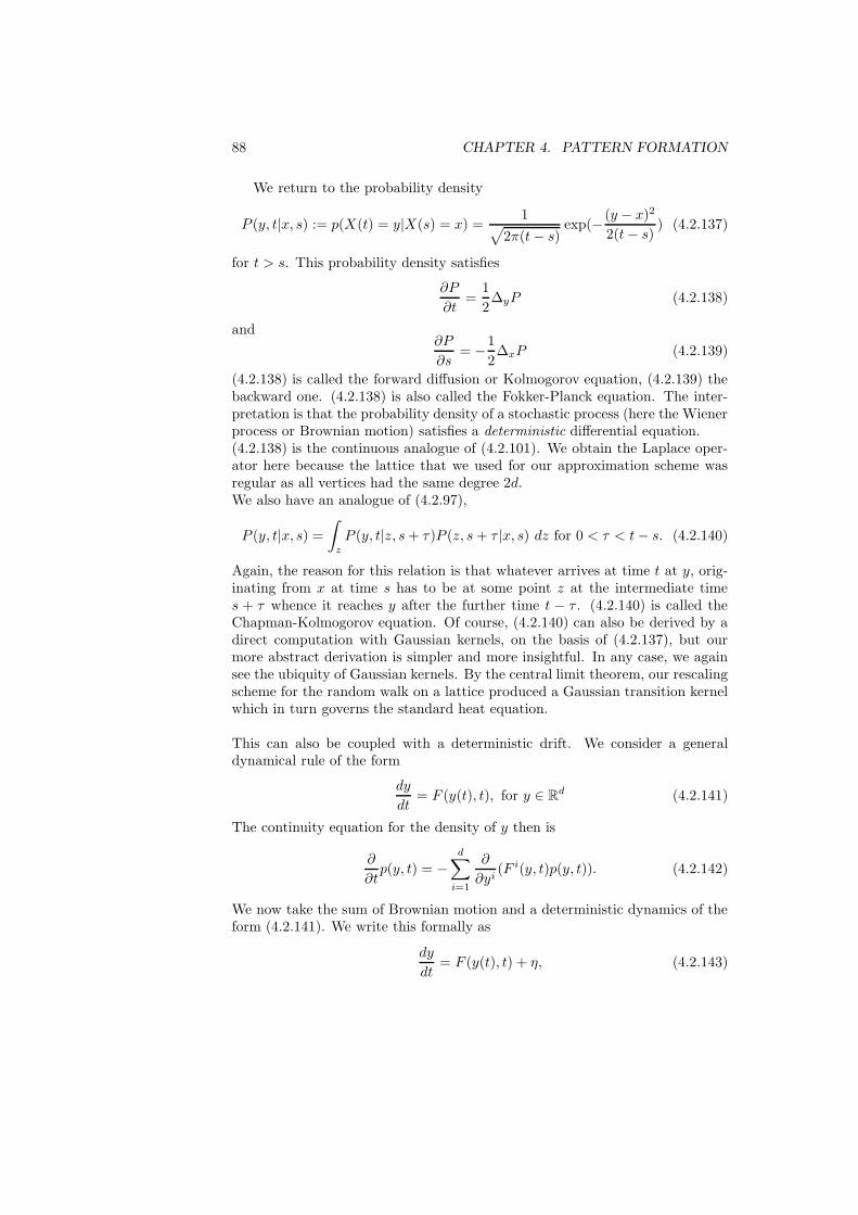
88 CHAPTER 4. PATTERN FORMATION
We return to the probability density
P (y, t|x, s) := p(X(t) = y|X(s) = x) =1
√
2π(t− s)exp(− (y − x)2
2(t− s)) (4.2.137)
for t > s. This probability density satisfies
∂P
∂t=
1
2∆yP (4.2.138)
and∂P
∂s= −1
2∆xP (4.2.139)
(4.2.138) is called the forward diffusion or Kolmogorov equation, (4.2.139) thebackward one. (4.2.138) is also called the Fokker-Planck equation. The inter-pretation is that the probability density of a stochastic process (here the Wienerprocess or Brownian motion) satisfies a deterministic differential equation.(4.2.138) is the continuous analogue of (4.2.101). We obtain the Laplace oper-ator here because the lattice that we used for our approximation scheme wasregular as all vertices had the same degree 2d.We also have an analogue of (4.2.97),
P (y, t|x, s) =
∫
z
P (y, t|z, s+ τ)P (z, s+ τ |x, s) dz for 0 < τ < t− s. (4.2.140)
Again, the reason for this relation is that whatever arrives at time t at y, orig-inating from x at time s has to be at some point z at the intermediate times + τ whence it reaches y after the further time t − τ . (4.2.140) is called theChapman-Kolmogorov equation. Of course, (4.2.140) can also be derived by adirect computation with Gaussian kernels, on the basis of (4.2.137), but ourmore abstract derivation is simpler and more insightful. In any case, we againsee the ubiquity of Gaussian kernels. By the central limit theorem, our rescalingscheme for the random walk on a lattice produced a Gaussian transition kernelwhich in turn governs the standard heat equation.
This can also be coupled with a deterministic drift. We consider a generaldynamical rule of the form
dy
dt= F (y(t), t), for y ∈ R
d (4.2.141)
The continuity equation for the density of y then is
∂
∂tp(y, t) = −
d∑
i=1
∂
∂yi(F i(y, t)p(y, t)). (4.2.142)
We now take the sum of Brownian motion and a deterministic dynamics of theform (4.2.141). We write this formally as
dy
dt= F (y(t), t) + η, (4.2.143)
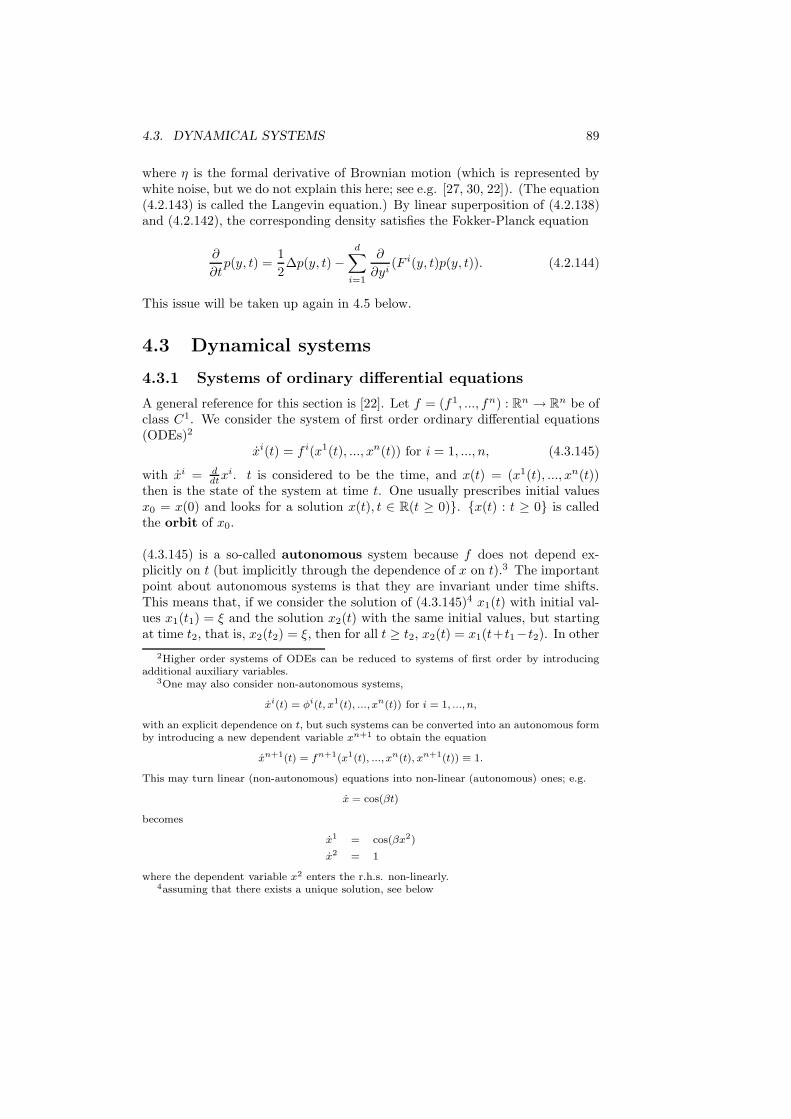
4.3. DYNAMICAL SYSTEMS 89
where η is the formal derivative of Brownian motion (which is represented bywhite noise, but we do not explain this here; see e.g. [27, 30, 22]). (The equation(4.2.143) is called the Langevin equation.) By linear superposition of (4.2.138)and (4.2.142), the corresponding density satisfies the Fokker-Planck equation
∂
∂tp(y, t) =
1
2∆p(y, t) −
d∑
i=1
∂
∂yi(F i(y, t)p(y, t)). (4.2.144)
This issue will be taken up again in 4.5 below.
4.3 Dynamical systems
4.3.1 Systems of ordinary differential equations
A general reference for this section is [22]. Let f = (f1, ..., fn) : Rn → R
n be ofclass C1. We consider the system of first order ordinary differential equations(ODEs)2
xi(t) = f i(x1(t), ..., xn(t)) for i = 1, ..., n, (4.3.145)
with xi = ddtx
i. t is considered to be the time, and x(t) = (x1(t), ..., xn(t))then is the state of the system at time t. One usually prescribes initial valuesx0 = x(0) and looks for a solution x(t), t ∈ R(t ≥ 0). x(t) : t ≥ 0 is calledthe orbit of x0.
(4.3.145) is a so-called autonomous system because f does not depend ex-plicitly on t (but implicitly through the dependence of x on t).3 The importantpoint about autonomous systems is that they are invariant under time shifts.This means that, if we consider the solution of (4.3.145)4 x1(t) with initial val-ues x1(t1) = ξ and the solution x2(t) with the same initial values, but startingat time t2, that is, x2(t2) = ξ, then for all t ≥ t2, x2(t) = x1(t+t1−t2). In other
2Higher order systems of ODEs can be reduced to systems of first order by introducingadditional auxiliary variables.
3One may also consider non-autonomous systems,
xi(t) = φi(t, x1(t), ..., xn(t)) for i = 1, ..., n,
with an explicit dependence on t, but such systems can be converted into an autonomous formby introducing a new dependent variable xn+1 to obtain the equation
xn+1(t) = fn+1(x1(t), ..., xn(t), xn+1(t)) ≡ 1.
This may turn linear (non-autonomous) equations into non-linear (autonomous) ones; e.g.
x = cos(βt)
becomes
x1 = cos(βx2)
x2 = 1
where the dependent variable x2 enters the r.h.s. non-linearly.4assuming that there exists a unique solution, see below
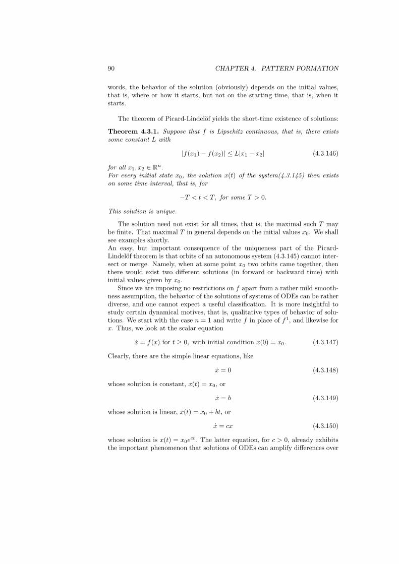
90 CHAPTER 4. PATTERN FORMATION
words, the behavior of the solution (obviously) depends on the initial values,that is, where or how it starts, but not on the starting time, that is, when itstarts.
The theorem of Picard-Lindelof yields the short-time existence of solutions:
Theorem 4.3.1. Suppose that f is Lipschitz continuous, that is, there existssome constant L with
|f(x1) − f(x2)| ≤ L|x1 − x2| (4.3.146)
for all x1, x2 ∈ Rn.
For every initial state x0, the solution x(t) of the system(4.3.145) then existson some time interval, that is, for
−T < t < T, for some T > 0.
This solution is unique.
The solution need not exist for all times, that is, the maximal such T maybe finite. That maximal T in general depends on the initial values x0. We shallsee examples shortly.An easy, but important consequence of the uniqueness part of the Picard-Lindelof theorem is that orbits of an autonomous system (4.3.145) cannot inter-sect or merge. Namely, when at some point x0 two orbits came together, thenthere would exist two different solutions (in forward or backward time) withinitial values given by x0.
Since we are imposing no restrictions on f apart from a rather mild smooth-ness assumption, the behavior of the solutions of systems of ODEs can be ratherdiverse, and one cannot expect a useful classification. It is more insightful tostudy certain dynamical motives, that is, qualitative types of behavior of solu-tions. We start with the case n = 1 and write f in place of f1, and likewise forx. Thus, we look at the scalar equation
x = f(x) for t ≥ 0, with initial condition x(0) = x0. (4.3.147)
Clearly, there are the simple linear equations, like
x = 0 (4.3.148)
whose solution is constant, x(t) = x0, or
x = b (4.3.149)
whose solution is linear, x(t) = x0 + bt, or
x = cx (4.3.150)
whose solution is x(t) = x0ect. The latter equation, for c > 0, already exhibits
the important phenomenon that solutions of ODEs can amplify differences over
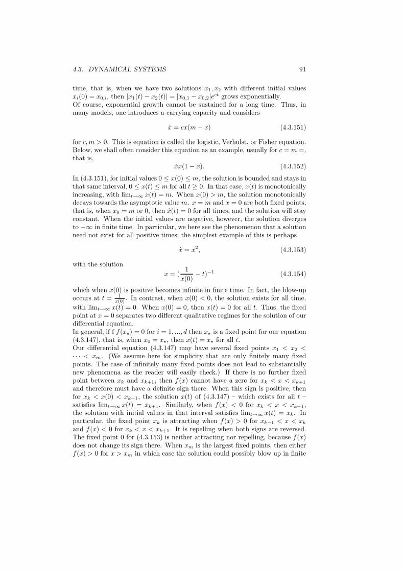
4.3. DYNAMICAL SYSTEMS 91
time, that is, when we have two solutions x1, x2 with different initial valuesxi(0) = x0,i, then |x1(t) − x2(t)| = |x0,1 − x0,2|ect grows exponentially.Of course, exponential growth cannot be sustained for a long time. Thus, inmany models, one introduces a carrying capacity and considers
x = cx(m− x) (4.3.151)
for c,m > 0. This is equation is called the logistic, Verhulst, or Fisher equation.Below, we shall often consider this equation as an example, usually for c = m =,that is,
xx(1 − x). (4.3.152)
In (4.3.151), for initial values 0 ≤ x(0) ≤ m, the solution is bounded and stays inthat same interval, 0 ≤ x(t) ≤ m for all t ≥ 0. In that case, x(t) is monotonicallyincreasing, with limt→∞ x(t) = m. When x(0) > m, the solution monotonicallydecays towards the asymptotic value m. x = m and x = 0 are both fixed points,that is, when x0 = m or 0, then x(t) = 0 for all times, and the solution will stayconstant. When the initial values are negative, however, the solution divergesto −∞ in finite time. In particular, we here see the phenomenon that a solutionneed not exist for all positive times; the simplest example of this is perhaps
x = x2, (4.3.153)
with the solution
x = (1
x(0)− t)−1 (4.3.154)
which when x(0) is positive becomes infinite in finite time. In fact, the blow-upoccurs at t = 1
x(0) . In contrast, when x(0) < 0, the solution exists for all time,
with limt→∞ x(t) = 0. When x(0) = 0, then x(t) = 0 for all t. Thus, the fixedpoint at x = 0 separates two different qualitative regimes for the solution of ourdifferential equation.In general, if f f(x⋆) = 0 for i = 1, ..., d then x⋆ is a fixed point for our equation(4.3.147), that is, when x0 = x⋆, then x(t) = x⋆ for all t.Our differential equation (4.3.147) may have several fixed points x1 < x2 <· · · < xm. (We assume here for simplicity that are only finitely many fixedpoints. The case of infinitely many fixed points does not lead to substantiallynew phenomena as the reader will easily check.) If there is no further fixedpoint between xk and xk+1, then f(x) cannot have a zero for xk < x < xk+1
and therefore must have a definite sign there. When this sign is positive, thenfor xk < x(0) < xk+1, the solution x(t) of (4.3.147) – which exists for all t –satisfies limt→∞ x(t) = xk+1. Similarly, when f(x) < 0 for xk < x < xk+1,the solution with initial values in that interval satisfies limt→∞ x(t) = xk. Inparticular, the fixed point xk is attracting when f(x) > 0 for xk−1 < x < xkand f(x) < 0 for xk < x < xk+1. It is repelling when both signs are reversed.The fixed point 0 for (4.3.153) is neither attracting nor repelling, because f(x)does not change its sign there. When xm is the largest fixed points, then eitherf(x) > 0 for x > xm in which case the solution could possibly blow up in finite
92 CHAPTER 4. PATTERN FORMATION
time, or f(x) < 0 for x > xm in which case the solution monotonically decays toxm for initial values x(0) > xm. The analogous situation holds when the initialvalues are smaller than the smallest fixed point.We can also formulate the following easy global existence result:
Theorem 4.3.2. We consider (4.3.147),
x = f(x) for t ≥ 0, with initial condition x(0) = x0 (4.3.155)
and assume that there exist numbers m < M with
f(m) > 0 and f(M) < 0 (4.3.156)
andm ≤ x0 ≤M. (4.3.157)
Then (for a Lipschitz continuous f as in (4.3.146)), the solution of (4.3.155)exists for all t ≥ 0.
Proof. The key observation is that the solution x(t) has to stay bounded aslong as it exists. Whenever it comes near the upper bound M , then x = f(x)becomes negative by (4.3.181), and therefore x(t), and when it comes near thelower bound m, it increases for the same reason. Therefore, we shall havem ≤ x(t) ≤M for all t for which the solution exists. By the theorem of Picard-Lindelof, we can then find some T > 0 such that for each t0 up to which thesolution exists, the solution of y(t) = f(y(t)) with y(0) = x(t0) exists for 0 ≤ tT .The important point here is that T here does not depend on x(t0) because thelatter is confined in the compact interval [m,M ]. x(t) = y(t − t0) then is thesolution of (4.3.155) on the interval [t0, t0 + T ]. This implies that the solutionhas to exist for all time (negative times, although not really our concern, arehandled by the same argument).
When the r.h.s. of (4.3.147) depends on some parameter λ, that is, we lookat
x = f(x, λ) (4.3.158)
then we expect a bifurcation, that is, a qualitative change of behavior of thesolutions at those parameter values λ = λ0 where the number of solutions xk of
f(x, λ) = 0 (4.3.159)
changes. For example, forx = x2 + λ (4.3.160)
λ = 0 is such a bifurcation point. For λ > 0, there is no fixed points, forλ = 0 there is one, namely 0, and for λ < 0, there are two, x = ±
√−λ.
Here, we already see the important principle that at generic (that is, typical)bifurcations, fixed always arise or disappear in pairs.For
x = λx− x3 (4.3.161)
4.3. DYNAMICAL SYSTEMS 93
λ = 0 is again a bifurcation point. For λ ≤ 0, x = 0 is the only fixed pointwhereas for λ > 0, we have additional ones at x = ±
√λ. The latter ones are
attracting whereas 0 is repelling for λ > 0, but attracting for λ ≤ 0.
The preceding already summarizes the main qualitative results about singleODEs of first order. For n > 1, the behavior of solutions of (4.3.145) can be-come richer and more interesting. When we move to dimension n = 2, two newphenomena emerge:
• saddle type fixed points in addition to attracting and repelling ones
• closed periodic orbits.
This is best understood within the context of some wider principles for theanalysis of dynamical systems:
1. identify the compact orbits (and perhaps other invariant sets) of the dy-namics,
2. linearize about them and
3. investigate their stability.
We now elaborate these points. The simplest case of an invariant set is a fixedpoint, that is, a point x⋆ for which the rhs of (4.3.145) vanishes, that is,
f i(x1⋆, . . . , x
n⋆ ) = 0. (4.3.162)
Typically, the investigation of a dynamical system starts with the identificationof these fixed points. We may assume x⋆ = 0 and study the linearized system
x(t) = Lx, with L =
(
∂f i
∂xj(x⋆)
)
i,j=1,...,n
. (4.3.163)
We consider the case n = 2 because the above principles already becomeclear there. The matrix L has either two real eigenvalues or two conjugatecomplex ones. When it can be diagonalized with two real eigenvalues λ1 andλ2, the after a linear change of coordinates, our linearized system becomes
x1(t) = λ1x1(t)
x2(t) = λ2x2(t), (4.3.164)
the solution of which obviously is
x1(t) = eλ1tx1(0)
x2(t) = eλ2tx2(0). (4.3.165)
If both eigenvalues are negative, then x(t) converges to the fixed point x⋆(= 0)exponentially while, in the case where both are positive, x(t) exponentiallyexpands.
94 CHAPTER 4. PATTERN FORMATION
In the first, attracting, case, x⋆ = 0 is called a node or sink, and it is astable fixed point for t → ∞, whereas in the second, repelling, case, called asource, it is unstable for t→ ∞. If the two eigenvalues have different signs, sayλ2 < 0 < λ1, then the fixed point x⋆0 is neither stable nor unstable. In fact, anyinitial point on the x2-axis converges to 0, while all other initial points divergeunder the flow. This is called a saddle. When one of the eigenvalues vanishes,the picture can get more complicated, and the behaviour of the linearized systemmay be different from the original one. Actually, this is already seen in the one-dimensional example
x = x2 (4.3.166)
the linearization of which at 0 is
x = 0. (4.3.167)
When, in contrast to the preceding cases, L has two complex conjugate eigen-values λ± iµ, then, after a linear change of coordinates again, we get the system
x(t) =
(
λ µ−µ λ
)
x(t), (4.3.168)
the solution of which is
x(t) = eλt(
cosµt sinµt− sinµt cosµt
)
x(0). (4.3.169)
For λ 6= 0, x(t) moves on a spiral (clockwise or counterclockwise, dependingon the sign of µ), exponentially towards 0 for λ < 0, exponentially expandingfor λ > 0. The case λ = 0 seems intermediate as the solution then moves ona circle about 0. This case is important for two reasons: it is the first non-trivial example of a compact orbit, and thus an invariant set, other than apoint. Secondly, this case λ = 0 is different from all previous cases, insofar asit is not structurally stable. This means that an arbitrarily small variation ofλ = 0 changes the qualitative behavior of the system. Even worse, even thequalitative behavior of the linearized system near the fixed point 0 is no longerthe same as that of the original system in case λ = 0. In a certain sense, thesetwo phenomena are related as we shall try to explain soon. Before doing that,we formulate a general
Definition 4.3.1. A fixed point x⋆ of (4.3.145) is called hyperbolic if all eigen-values of the linearized system have nonvanishing real part.
The qualitative dynamical behaviour near a hyperbolic fixed point is struc-turally stable in the sense that it is not affected by sufficiently small perturba-tions or parameter variations (like the eigenvalues of the linearized system), andthat it is the same as the one of the linearized system – in fact, the differencebetween the original and the linearized system is such a small perturbation that
4.3. DYNAMICAL SYSTEMS 95
does not change the qualitative behaviour.We now look into a non-hyperbolic situation and consider the linear system
x = y + λx (4.3.170)
y = −x+ λy. (4.3.171)
The eigenvalues are λ± i, with imaginary part 6= 0, and real part = 0 for λ = 0.We may consider λ as a bifurcation parameter, and λ = 0 as a bifurcationvalue where the qualitative behaviour of the solution changes. Here, a pairof complex conjugate nonzero eigenvalues crosses the imaginary axis. This isthe characteristic criterion for the so-called Hopf bifurcation as we shall nowexplain.In the linear system, at λ = 0 all orbits are periodic, namely circles, about (0, 0),while for λ 6= 0 there is no periodic orbit at all.(4.3.170) is the linearization at (0, 0) of
x = y − x (x2 + y2 − λ) (4.3.172)
y = −x− y (x2 + y2 − λ) (4.3.173)
For this system, (0, 0) is a fixed point for all parameter values λ. For λ 6= 0, thesituation is hyperbolic and therefore qualitatively the same as in the linearizedsystem. For λ < 0, the fixed point is globally exponentially attracting. Whilethis can be deduced from general principles, we can, of course, also see it directly,and this gives us the opportunity to introduce another useful tool, a Lyapunovfunction which by definition is a function that is strictly decreasing along everyflow line. Here, such a Lyapunov function is given by log(x2 + y2) since we have
d
dtlog(x2 + y2) = 2(−x2 − y2 + λ) ≤ 2λ < 0. (4.3.174)
Thus, log(x2 + y2) decreases along every flow line, and then so does x2 + y2,and therefore each flow line has to lead to (0, 0). As already pointed out, thisis a structurally stable situation that is invariant under small perturbations of λ.
For λ = 0, (0, 0) is still globally attracting, but no longer exponentially so.We still have
d
dtlog(x2 + y2) < 0 for (x, y) 6= (0, 0), (4.3.175)
but this expression is no longer bounded away from 0. Thus, we see again thatthe situation at λ = 0 is not structurally stable.
For λ > 0, while the situation near (0, 0) is again structurally stable, aninteresting global phenomenon emerges away from (0, 0). (0, 0) is repelling, andthere exists a periodic orbit x2 + y2 = λ that is attracting. To understand this,we consider our Lyapunov function:
d
dtlog(x2 + y2)
> 0 for x2 + y2 < λ
= 0 for x2 + y2 = λ
< 0 for x2 + y2 > λ.
(4.3.176)
96 CHAPTER 4. PATTERN FORMATION
Thus, when we are on the circle x2 + y2 = λ, we stay there and since, x and ydo not vanish there, it is a nontrivial periodic orbit. When we are outside orinside that circle, we move towards it.We thus obtain a family, depending on λ, of periodic orbits that emerge fromthe fixed point at the transition from λ = 0 to λ > 0. This family of periodicorbits represents a structurally stable bifurcation, that is, such a family remainsunder perturbations of the above system.In contrast to this behaviour, in the linear system, at λ = 0 all orbits are peri-odic, namely circles, about (0, 0), while for λ 6= 0 there is no periodic orbit atall. Thus, here the whole family of periodic orbits is concentrated at a singleparameter value, while when the linear system is perturbed by a higher orderterm, that family gets distributed among different parameter values. The situ-ation at λ = 0 itself is not structurally stable while the behaviour of the wholefamily is, namely the emergence of a family of periodic orbits at the transitionfrom an attracting to a repelling fixed point.
We next consider another system with the same linearization (4.3.170), (4.3.171)as the preceding one, (4.3.172), (4.3.173),
x = y − x ((x2 + y2)2 − 2(x2 + y2) − λ) (4.3.177)
y = −x− y ((x2 + y2)2 − 2(x2 + y2) − λ) (4.3.178)
depending on a real parameter λ as before. We now have
d
dtlog(x2 + y2) = 2(−(x2 + y2)2 + 2(x2 + y2) + λ). (4.3.179)
This becomes 0 when
x2 + y2 = 1 ±√
1 + λ.
Thus, whenever this value is real and nonnegative, we obtain that x2 + y2 re-mains constant along a solution, that is, the orbit is a circle. When λ is smallerthan −1, no such solution exists. For λ = −1, we find precisely one solutionwhereas, for −1 < λ < 0, we obtain two solutions, of radii 0 < ρ1 < ρ2, say.The right-hand side of (4.3.179) is negative for 0 < ρ :=
√
x2 + y2 < ρ1, butpositive for ρ1 < ρ < ρ2 and negative again beyond ρ2. Thus, the orbit atρ1 is repelling whereas the one at ρ2 is attracting. When λ increases to 0, therepelling periodic orbit at ρ1 moves into the attracting fixed point at 0. When λthen becomes positive, both the repelling periodic orbit and the attracting fixedpoint disappear, or, more precisely, the latter turns into a repelling fixed point.Only the attracting periodic orbit at ρ2 remains. The solution of our system ofODEs then has no option but to move away from the no longer attracting fixedpoint at 0 to the periodic orbit at ρ2.The first bifurcation, the one of (4.3.170), (4.3.171), where a stable fixed pointcontinuously changed into a stable periodic orbit was a so-called supercriticalHopf bifurcation. In contrast to this, in a subcritical Hopf bifurcation, as exem-plified by (4.3.177), (4.3.178), an unstable periodic orbit coalesces into a stable
4.3. DYNAMICAL SYSTEMS 97
fixed point so that the latter becomes repelling and no stable orbit is presentanymore in its vicinity when the relevant parameter passes the bifurcation value.The linearization at 0 is the same for both examples, the supercritical and thesubcritical Hopf bifurcation. The linearization possesses a pair of complex con-jugate eigenvalues whose real parts vanish at the bifurcation point. In fact, bythe theorem of E.Hopf, this is precisely the criterion for such a bifurcation wherea stable fixed point bifurcates into a family of periodic orbits.
The preceding examples essentially cover the qualitative types of behaviourof two-dimensional systems of ODEs. This is essentially a consequence of theprinciple observed as a corollary of the Picard-Lindelof theorem that two orbitscan never intersect or merge. In higher dimensions, however, (even though thatprinciple is still in force) the behaviour can get more complicated, and in factdefies a complete classification.In any case, however, we have an existence result of the type of Theorem 4.3.2.
Theorem 4.3.3. We consider for x = (x1, . . . , xn) and f = (f1, . . . , fn),
x = f(x) for t ≥ 0, with initial condition x(0) = x0 (4.3.180)
and assume that there exist numbers mα < Mα for α = 1, . . . , n with
f(x1, . . . , xα−1,mα, xα+1, . . . , xn) > 0 and f(x1, . . . , xα−1,Mα, xα+1, . . . , xn) < 0(4.3.181)
whenever mβ ≤ xβ ≤Mβ for all β = 1, . . . , n, and also
mbeta ≤ xβ0 ≤Mβ . (4.3.182)
Then (for a Lipschitz continuous f), the solution of (4.3.155) exists for all t ≥ 0.
The proof proceeds as the one of Theorem 4.3.2.
We now exhibit several systems of ODEs that are important as models at vari-ous biological scales.
1) Biochemical kinetics:References here are [28], [24]. The basis here is the law of mass action whichstates the reaction rate of a chemical reaction is proportional to the concentra-tions of the reactants raised to the number in which they enter the reaction.That expression is proportional to the collision probability for the reactants.For the simple reaction
S1 + S2 2P (4.3.183)
when k+ is the rate constant for the forward reaction that converts S1 +S2 into2P and k− is the one for the backward reaction and if we denote the respectiveconcentrations by s1, s2, p, then
s1 = s2 = −k+s1s2 + k−p2 (4.3.184)
p = 2(k+s1s2 − k−p2). (4.3.185)
98 CHAPTER 4. PATTERN FORMATION
Enzymatic reactions are of particular importance. The prototype is
E + S ES → E + P. (4.3.186)
Here, the substrate S and the enzymeE first form the enzyme-substrate complexES in a reversible manner with forward and backward rate constants k1, k−1,resp., and then the product P is irreversibly released from the enzyme E withrate constant k2. When we denote the concentrations of E,S,ES, P by e, s, c, p,resp., we obtain the system of ODEs
s = −k1es+ k−1c (4.3.187)
e = −k1es+ (k−1 + k2)c (4.3.188)
c = k1es− (k−1 + k2)c (4.3.189)
p = k2c. (4.3.190)
We observe that p does not appear on the r.h.s of this system. Thus, we needonly solve the first 3 equations. p then is obtained by a simple integration.Moreover, the second and third equations are dependent, and we conclude
e(t) + c(t) ≡ e0 (4.3.191)
a constant.Based on the small amount of enzyme needed for such reactions, the Michaelis-Menten theory makes the assumption of a quasi-steady state for the complexES,
c = 0. (4.3.192)
This is mathematically not unproblematic and requires a singular perturbationanalysis, see [28], but here we simply observe the consequence
c =k1e0s
k1s+ k−1 + k2. (4.3.193)
We now move from the molecular to the cellular level and as our next exampleconsider the2) Hodgkin-Huxley model for the firing of neurons:The main variable is the potential V of the neuron, satisfying the ODE
CdV
dt= Ie − Ii (4.3.194)
where C is the capacitance of the membrane and Ie and Ii are the external andinternal currents. The internal current in turn satisfies the equation
Ii = g0(V − V0) + g1m3h(V − V1) + g2n
4(V − V2), (4.3.195)
where g0, g1, g2 > 0 and V0, V1, V2 are constants whereas m,n, h are gatingvariables corresponding to activation of sodium (Na+), activation of potassium
4.3. DYNAMICAL SYSTEMS 99
(K+), and inactivation of Na+, resp. Normalizations are such that the gatingvariables always take their values between 0 and 1 so that the can be interpretedas the probabilities for the corresponding type of channel to be open.(4.3.194) and (4.3.195) combine to become
CdV
dt= Ie − (g0(V − V0) + g1m
3h(V − V1) + g2n4(V − V2)). (4.3.196)
Whereas Ie is treated as an external parameter, the internal dynamical regimescrucially depend on the signs of the three terms in (4.3.196) contributing to Ii.Before going into details, we then formulate a fourth principle for the investiga-tion of systems of ODEs:
4. determine the signs of the diverse summands into which f i may be de-composed on the right hand side of (4.3.145) and assess their contributionon the global behaviour of the solution.
Before proceeding, however, we need to clarify the roles of the gating variables.m,n, h satisfy differential equations of the form
τy(V )dy
dt= y∞(V ) − y (4.3.197)
with the limiting value y∞(V ) and the time constant τy(V ) indicating the timescale on which the corresponding gating variable varies. A simpler model wouldconsist of taking y directly as a function of V , equal to the equilibrium value,that is, y = y∞(V ). The model of Hodgkin-Huxley instead introduces someadditional temporal dynamics where y relaxes to that equilibrium value on thetime scale described by τy(V ). Thus, in particular, it does not follow changesin V instantaneously, but needs some time to adapt.The Hodgkin-Huxley systems then consists of 4 differential equations, namely(4.3.196) for the voltage V and three equations of type (4.3.197) for the threegating variables.It is important for the dynamics of the Hodgkin-Huxley model that while m∞and n∞ are increasing functions of V (m∞ starts to rise only at a somewhathigher value of V (around -80 mV) than n∞), h∞ is a decreasing function.Moreover, the time constant τm is much smaller than the time constants τn, τh(which peak at values of V between -80 and -70 mV), and so m changes muchfaster than n and h, in fact on the same scale as V .The reversal potentials in (4.3.195) are
V1 = 50mV (4.3.198)
V2 = −77mV (4.3.199)
V0 = −54.4mV. (4.3.200)
We now present a qualitative discussion of the dynamics of the Hodgkin-Huxleymodel. Suppose the system initially is at rest near V0. Then h = h∞(V0) andn = n∞(V0) are positive (in the order of magnitude 1/2) while m = m∞(V0) is
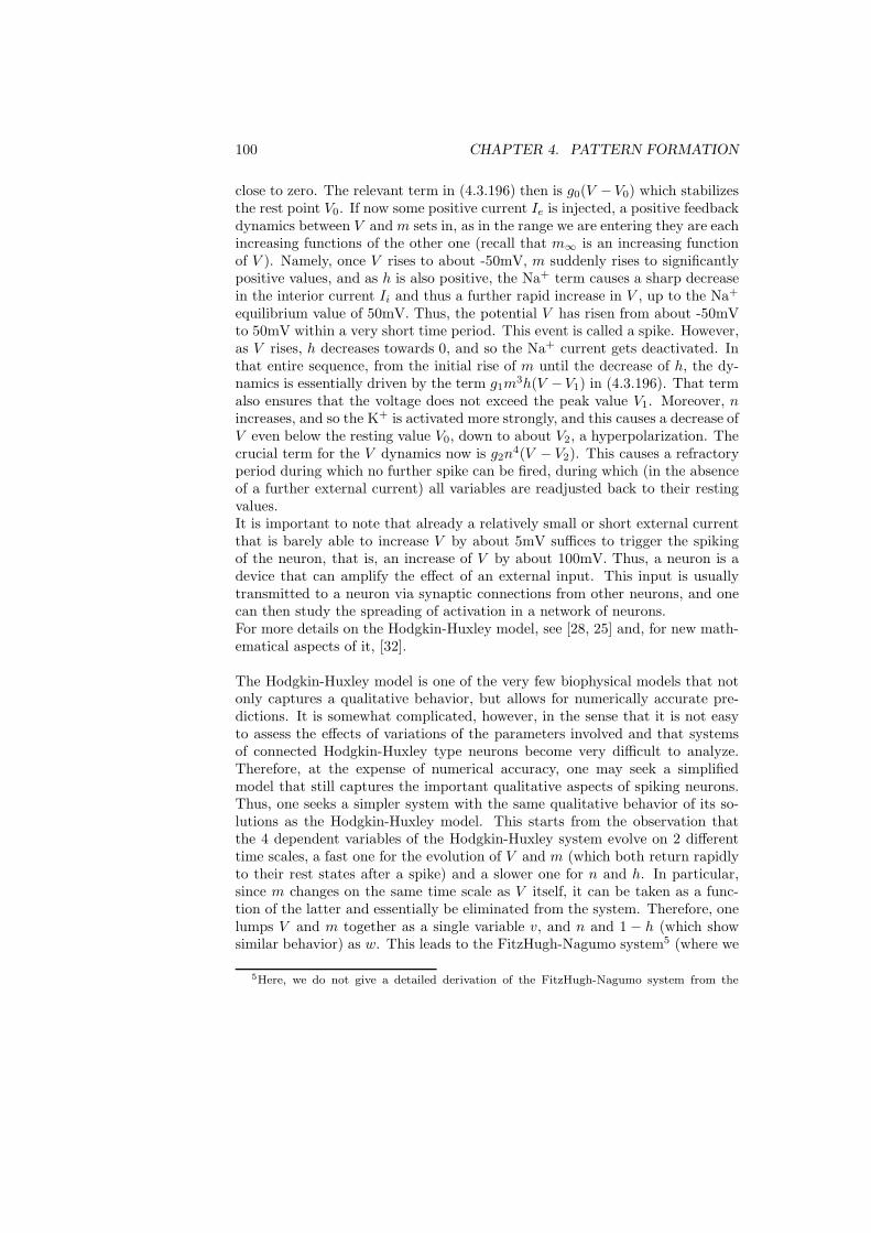
100 CHAPTER 4. PATTERN FORMATION
close to zero. The relevant term in (4.3.196) then is g0(V −V0) which stabilizesthe rest point V0. If now some positive current Ie is injected, a positive feedbackdynamics between V and m sets in, as in the range we are entering they are eachincreasing functions of the other one (recall that m∞ is an increasing functionof V ). Namely, once V rises to about -50mV, m suddenly rises to significantlypositive values, and as h is also positive, the Na+ term causes a sharp decreasein the interior current Ii and thus a further rapid increase in V , up to the Na+
equilibrium value of 50mV. Thus, the potential V has risen from about -50mVto 50mV within a very short time period. This event is called a spike. However,as V rises, h decreases towards 0, and so the Na+ current gets deactivated. Inthat entire sequence, from the initial rise of m until the decrease of h, the dy-namics is essentially driven by the term g1m
3h(V −V1) in (4.3.196). That termalso ensures that the voltage does not exceed the peak value V1. Moreover, nincreases, and so the K+ is activated more strongly, and this causes a decrease ofV even below the resting value V0, down to about V2, a hyperpolarization. Thecrucial term for the V dynamics now is g2n
4(V − V2). This causes a refractoryperiod during which no further spike can be fired, during which (in the absenceof a further external current) all variables are readjusted back to their restingvalues.It is important to note that already a relatively small or short external currentthat is barely able to increase V by about 5mV suffices to trigger the spikingof the neuron, that is, an increase of V by about 100mV. Thus, a neuron is adevice that can amplify the effect of an external input. This input is usuallytransmitted to a neuron via synaptic connections from other neurons, and onecan then study the spreading of activation in a network of neurons.For more details on the Hodgkin-Huxley model, see [28, 25] and, for new math-ematical aspects of it, [32].
The Hodgkin-Huxley model is one of the very few biophysical models that notonly captures a qualitative behavior, but allows for numerically accurate pre-dictions. It is somewhat complicated, however, in the sense that it is not easyto assess the effects of variations of the parameters involved and that systemsof connected Hodgkin-Huxley type neurons become very difficult to analyze.Therefore, at the expense of numerical accuracy, one may seek a simplifiedmodel that still captures the important qualitative aspects of spiking neurons.Thus, one seeks a simpler system with the same qualitative behavior of its so-lutions as the Hodgkin-Huxley model. This starts from the observation thatthe 4 dependent variables of the Hodgkin-Huxley system evolve on 2 differenttime scales, a fast one for the evolution of V and m (which both return rapidlyto their rest states after a spike) and a slower one for n and h. In particular,since m changes on the same time scale as V itself, it can be taken as a func-tion of the latter and essentially be eliminated from the system. Therefore, onelumps V and m together as a single variable v, and n and 1 − h (which showsimilar behavior) as w. This leads to the FitzHugh-Nagumo system5 (where we
5Here, we do not give a detailed derivation of the FitzHugh-Nagumo system from the
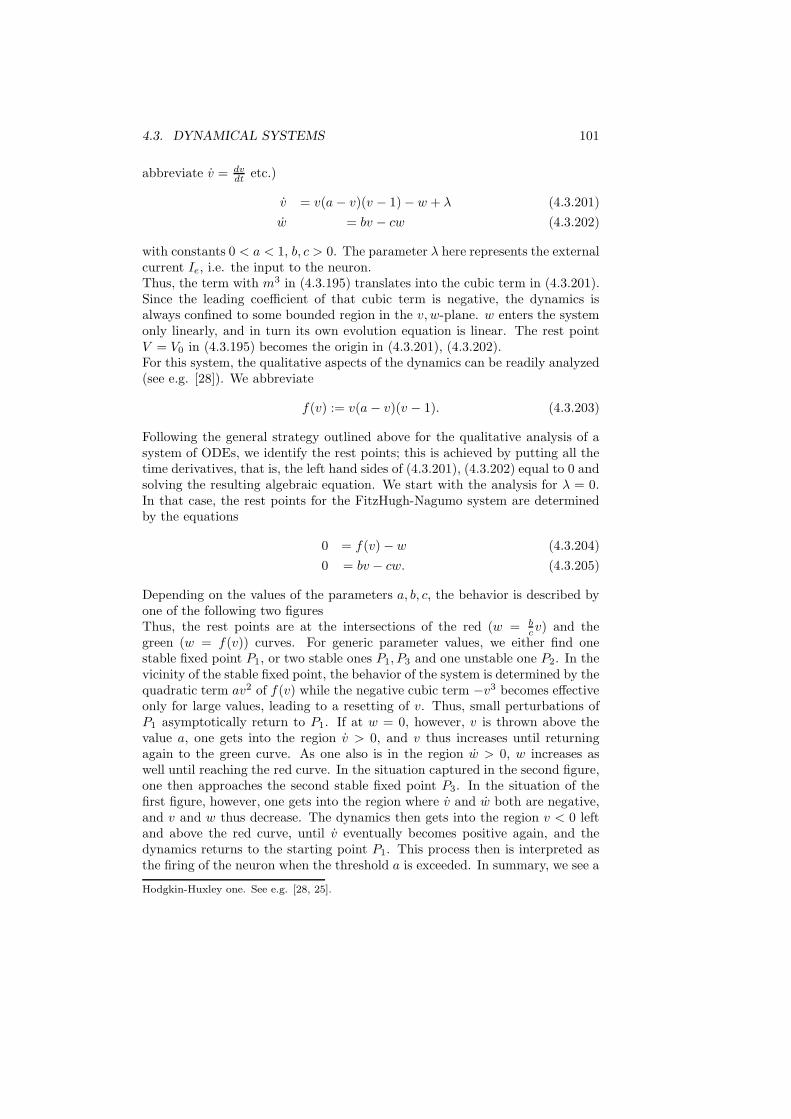
4.3. DYNAMICAL SYSTEMS 101
abbreviate v = dvdt etc.)
v = v(a− v)(v − 1) − w + λ (4.3.201)
w = bv − cw (4.3.202)
with constants 0 < a < 1, b, c > 0. The parameter λ here represents the externalcurrent Ie, i.e. the input to the neuron.Thus, the term with m3 in (4.3.195) translates into the cubic term in (4.3.201).Since the leading coefficient of that cubic term is negative, the dynamics isalways confined to some bounded region in the v, w-plane. w enters the systemonly linearly, and in turn its own evolution equation is linear. The rest pointV = V0 in (4.3.195) becomes the origin in (4.3.201), (4.3.202).For this system, the qualitative aspects of the dynamics can be readily analyzed(see e.g. [28]). We abbreviate
f(v) := v(a− v)(v − 1). (4.3.203)
Following the general strategy outlined above for the qualitative analysis of asystem of ODEs, we identify the rest points; this is achieved by putting all thetime derivatives, that is, the left hand sides of (4.3.201), (4.3.202) equal to 0 andsolving the resulting algebraic equation. We start with the analysis for λ = 0.In that case, the rest points for the FitzHugh-Nagumo system are determinedby the equations
0 = f(v) − w (4.3.204)
0 = bv − cw. (4.3.205)
Depending on the values of the parameters a, b, c, the behavior is described byone of the following two figuresThus, the rest points are at the intersections of the red (w = b
cv) and thegreen (w = f(v)) curves. For generic parameter values, we either find onestable fixed point P1, or two stable ones P1, P3 and one unstable one P2. In thevicinity of the stable fixed point, the behavior of the system is determined by thequadratic term av2 of f(v) while the negative cubic term −v3 becomes effectiveonly for large values, leading to a resetting of v. Thus, small perturbations ofP1 asymptotically return to P1. If at w = 0, however, v is thrown above thevalue a, one gets into the region v > 0, and v thus increases until returningagain to the green curve. As one also is in the region w > 0, w increases aswell until reaching the red curve. In the situation captured in the second figure,one then approaches the second stable fixed point P3. In the situation of thefirst figure, however, one gets into the region where v and w both are negative,and v and w thus decrease. The dynamics then gets into the region v < 0 leftand above the red curve, until v eventually becomes positive again, and thedynamics returns to the starting point P1. This process then is interpreted asthe firing of the neuron when the threshold a is exceeded. In summary, we see a
Hodgkin-Huxley one. See e.g. [28, 25].
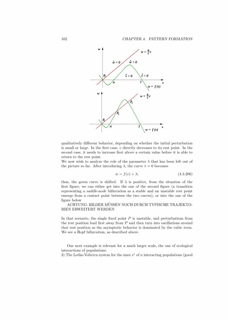
102 CHAPTER 4. PATTERN FORMATION
w = bc v
w > 0
w
p1
w < 0
a w = f (v)
v > 0 v < 0
1 v
w = bc v
w
p1
p
p
2
3
vw = f (v)
a 1
qualitatively different behavior, depending on whether the initial perturbationis small or large. In the first case, v directly decreases to its rest point. In thesecond case, it needs to increase first above a certain value before it is able toreturn to the rest point.We now wish to analyze the role of the parameter λ that has been left out ofthe picture so far. After introducing λ, the curve v = 0 becomes
w = f(v) + λ; (4.3.206)
thus, the green curve is shifted. If λ is positive, from the situation of thefirst figure, we can either get into the one of the second figure (a transitionrepresenting a saddle-node bifurcation as a stable and an unstable rest pointemerge from a contact point between the two curves), or into the one of thefigure below
ACHTUNG: BILDER MUSSEN NOCH DURCH TYPISCHE TRAJEKTO-RIEN ERWEITERT WERDEN
In that scenario, the single fixed point P is unstable, and perturbations fromthe rest position lead first away from P and then turn into oscillations aroundthat rest position as the asymptotic behavior is dominated by the cubic term.We see a Hopf bifurcation, as described above.
Our next example is relevant for a much larger scale, the one of ecologicalinteractions of populations:3) The Lotka-Volterra system for the sizes xi of n interacting populations (good
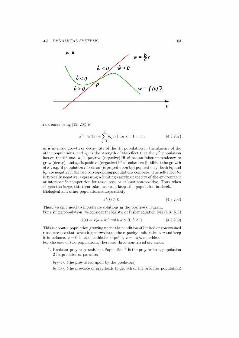
4.3. DYNAMICAL SYSTEMS 103
w = bc v
w
w < 0 w > 0
p
v
v < 0
v > 0 w = f (v)+ λ
references being [19, 20]) is
xi = xi(ai +
d∑
j=1
bijxj) for i = 1, ..., n. (4.3.207)
ai is intrinsic growth or decay rate of the ith population in the absence of theother populations, and bij is the strength of the effect that the jth populationhas on the ith one. a1 is positive (negative) iff xi has an inherent tendency togrow (decay), and bij is positive (negative) iff xj enhances (inhibits) the growthof xi, e.g. if population i feeds on (is preyed upon by) population j; both bij andbji are negative if the two corresponding populations compete. The self-effect biiis typically negative, expressing a limiting carrying capacity of the environmentor interspecific competition for ressources, or at least non-positive. Thus, whenxi gets too large, this term takes over and keeps the population in check.Biological and other populations always satisfy
xi(t) ≥ 0. (4.3.208)
Thus, we only need to investigate solutions in the positive quadrant.For a single population, we consider the logistic or Fisher equation (see (4.3.151))
x(t) = x(a+ bx) with a > 0, b < 0. (4.3.209)
This is about a population growing under the condition of limited or constrainedressources, so that, when it gets two large, the capacity limits take over and keepit in balance. x = 0 is an unstable fixed point, x = −a/b a stable one.For the case of two populations, there are three non-trivial scenarios:
1. Predator-prey or parasitism: Population 1 is the prey or host, population2 its predator or parasite:
b12 < 0 (the prey is fed upon by the predators)
b21 > 0 (the presence of prey leads to growth of the predator population).
104 CHAPTER 4. PATTERN FORMATION
In the predator-prey scenario, one also typically has
a1 > 0 (the prey population grows in the absence of predators)
a2 < 0 (the predator population decays in the absence of prey).
2. Competition
b12 < 0 and b21 < 0 (the two populations inhibit each other).
3. Symbiosis:
b12 > 0 and b21 > 0 (the two populations support each other).
We now look at the example of the two-dimensional predator-prey modelwithout intraspecific competition, that is, we have a prey population of size x1
and a predator population of size x2,
x1 = x1(a1 + b12x2) (4.3.210)
x2 = x2(a2 + b21x1),
witha1 > 0, a2 < 0, b12 < 0, b21 > 0.
We first observe that (x1, x2) = (0, 0) is a fixed point. Linearization showsthat this fixed point is a saddle. On the x1-axis, the solution expands accordingto x1(t) = x1(0)ea1t, x2(t) = 0, whereas it contracts along the x2-axis as a2 < 0,x1(t) = 0, x2(t) = x2(0)ea2t. In particular, since the two axes are orbits, thesolution cannot cross them, that is, when starting with non-negative values, itwill never turn negative, in accordance with (4.3.208).Another fixed point is
x1 = − a2
b21, x2 = − a1
b12(4.3.211)
All the other orbits in the positive quadrant are periodic, circling this fixed pointcounterclockwise. This is seen either from the local behavior of the trajectoriesnear (0, 0) or by looking at
V (x1, x2) := b21(x1 log x1 − x1) − b12(x
2 log x2 − x2), (4.3.212)
which satisfies
d
dtV (x1(t), x2(t)) = −a2
x1
x1− b21x
1 + a1x2
x2+ b12x
2 by (4.3.211)
= 0 by (4.3.212).
Thus, V (x1, x2) is a constant of motion. V attains its unique maximum at(x1, x2), and so the curves V (x1, x2) ≡ constant are circles, that is, closed curves,around this point. The motion on such a circle is counterclockwise because in
4.3. DYNAMICAL SYSTEMS 105
the case x1(t) > x1, x2(t) > x2 for example, we have x1(t) < 0, x2(t) > 0.On the line x1 = x1, x2(t) = 0, that is, x2 stays constant there, and on x2 = x2,x1 stays constant.Thus, the prey and predator populations oscillate periodically in this model.
The behaviour of the preceding system with its family of periodic orbits is notstable under small perturbations, as we already know from our discussion of theHopf bifurcation above. For example when we include intraspecific competition,obtaining the system
x1 = x1(a1 + b11x1 + b12x
2)
x2 = x2(a2 + b21x1 + b22x
2) (4.3.213)
where we now assume
b11 < 0 (the members of the prey population compete for food or other ressources)
b22 ≤ 0,
the qualitative behaviour of the system becomes different. We find a second fixedpoint on the positive x1-axis, (− a1
b11, 0). This fixed point is always attractive for
x1, because in case x2(t) = 0, we have the logistic equation (4.3.209)
x1(t) = x1(a1 + b11x1) with a1 > 0, b11 < 0. (4.3.214)
It is also attractive for x2 when
a2b11 − a1b21 > 0.
In that case, there is no other fixed point in the positive quadrant, and in factfor any solution
limt→∞
x2(t) = 0.
The predator becomes extinct. Thus, we conclude that a small intraspecificcompetition among the prey population may lead to the extinction of theirpredators.If, however,
a2b11 − a1b21 < 0,
then
x1 =a2b12 − a1b22b11b22 − b12b21
> 0
x2 =a1b21 − a2b11b11b22 − b12b21
> 0
is a fixed point in the positive quadrant.With V (x1, x2) as in (4.3.212),
d
dtV (x1(t), x2(t)) = −b11b21(x1 − x1(t))2 + b12b22(x
2 − x2(t))2 > 0,
106 CHAPTER 4. PATTERN FORMATION
unless (x1, x2) = (x1, x2) in which case this derivative vanishes. Thus, V (x1(t), x2(t))increases along every orbit, and equilibrium is possible only at its maximum,at the fixed point (x1, x2). The orbits in the positive quadrant then all spiralcounterclockwise towards this fixed point. Thus, in this case, the two popula-tions eventually converge to this fixed point.We have observed that an arbitrarily small variation of the original system, hereby introducing competition among the hosts, changes the global qualitative be-havior of the solutions. Therefore, one cannot expect that this model leads toa qualitatively robust and structurally stable behavior, and predictions basedon such a model need to be examined with great care. Volterra originally in-troduced the model to explain the periodic oscillations in two fish populationsin the Adriatic, one preying upon the other one. As it turned out, however,this periodic behavior is not caused by an interaction of the two populationsaccording to the model, but rather by periodic changes in the water tempera-ture, that is, by external periodic forcing. Although the model therefore failsits original purpose, it has become useful at a more abstract level, for gametheoretic models of interactions inside populations, see [19, 20].
4.4 Reaction-diffusion systems
References: [34, 28, 21].
4.4.1 Reaction-diffusion equations
Let Ω ⊂ Rd be open and bounded.
We consider the equation
ut(x, t) = ∆u(x, t) + f(x, t, u) for x ∈ Ω, 0 < t < T (4.4.1)
u(x, 0) = φ(x) for x ∈ Ω
u(y, t) = g(y, t) for y ∈ ∂Ω, 0 < t < T
for continuous and bounded initial and boundary values and a differentiablereaction term f .We can consider this is a generalization of
1. either the ODEut(t) = f(t, u), (4.4.2)
(at least in the case where the function f in (4.4.1) does not depend onx), that is, of an equation that does not depend on the spatial variable xand therefore describes a spatially homogeneous state,
2. or the linear heat equation
ut(x, t) = ∆u(x, t), (4.4.3)
that is, of an equation that describes a linear diffusion process in space.
4.4. REACTION-DIFFUSION SYSTEMS 107
The first equation describes a reaction process, and thus, a reaction-diffusionequation models reaction processes taking place at all points in space simul-taneously and being diffusively coupled. It turns out that such an interplayof reaction and diffusion processes can lead to more interesting patterns thaneither of these processes alone.In order to understand the relationship between the two processes better, we canalso introduce a diffusion coefficient d and consider the more general equation
ut(x, t) = d∆u(x, t) + f(x, t, u), u(x, 0) = φ(x) (4.4.4)
When d = 0, we have a system of ODEs indexed by the points x, but withoutany coupling or interaction between those points. Thus, at each point x, thedynamics is driven by the reaction term, and the result depends only on theinitial condition φ(x) at that particular x. When we let d → ∞, we obtainan equation for the spatially integrated variables, that is, a single ODE for thespatially averaged quantity, and there will be no variation between the differentpoints x. In general, in physical and biological processes, conservation rules willlimit growth, and growth at one point x then is only possible at the expense ofother points. In principle, a reaction-diffusion equation can then lead to optimalresource allocation in the limit t → ∞. The time scale on which this takes placewill depend on the diffusion coefficient d.Recalling (4.3.155), let us consider
ut = ∆u+ u(1 − u), (4.4.5)
for u = u(x, t), that is, the logistic (Verhulst, Fisher) equation with a diffusionterm. This equation is sometimes called the Kolmogorov-Fisher equation. Itcan serve as a model for a population in a uniform habitat with limited capacitythat reproduces and diffuses in space. As such, we expect that the behavior ofa solution u(x, t) at a point x is not very different from the solution of theODE yt(t) = y(t)(1 − y(t)) with initial value y(0) = u(x, 0). In particular, weexpect that a solution u(x, t) with a positive initial value converges to 1 fort to∞, unless this prevented by the boundary condition. However, there willbe diffusion between the different x ∈ Ω, and this may decrease the differencesin their respective initial conditions faster than the dynamical evolution by thereaction term alone. This effect becomes more important when we consider thespatially inhomogeneous equation
ut(x, t) = ∆u(x, t) + u(x, t)(a(x) − b(x)u(x, t)) (4.4.6)
for positive functions a, b. Thus, the intrinsic growth rate and the capacitylimitations depend on x. Now, the stable equilibrium point for the reaction
term, u = a(x)b(x) , depends on the spatial position x. Without diffusion, at every
x then in the limit t→ ∞, this equilibrium would be obtained. With diffusion,however, we expect some harmonization between the higher and lower values ofthat equilibrium.
108 CHAPTER 4. PATTERN FORMATION
In applications, the dependent variable u typically describes some density,and therefore only non-negative solutions u will be meaningful.
Example:
ut(x, t) = ∆u(x, t) + u2(x, t) for x ∈ Ω, 0 < t (4.4.7)
u(x, 0) = φ(x) for x ∈ Ω
u(y, t) = 0 for y ∈ ∂Ω, 0 < t
with
φ > 0 in Ω. (4.4.8)
We recall that the ODE
ut(t) = u2(t) (4.4.9)
for positive initial value u(0) did blow up in finite time (cf. (4.3.153), (4.3.154)),that is, did not possess a solution that exists for all t > 0. We shall now showthat the same happens for (4.4.7) provided the initial values φ are sufficientlylarge. To make that condition precise, we recall the first Dirichlet eigenvalue λ1
and the corresponding eigenfunction u1 from Theorem 4.1.1, solving
∆u1 + λ1u1 = 0, u1 = 0 on ∂Ω,
and recall that, by (4.1.69),
u1(x) > 0 for x ∈ Ω; (4.4.10)
we may normalize u1 to satisfy
∫
Ω
u1(x)dx = 1. (4.4.11)
By the maximum principle Lemma 4.1.2, because of (4.4.8), we have
u(x, t) > 0 for x ∈ Ω, 0 < t. (4.4.12)
We look at the auxiliary function
y(t) :=
∫
Ω
u(x, t)u1(x)dx (4.4.13)
which satisfies
y(t) =∫
Ωut(x, t)u1(x)dx =
∫
Ω(∆u(x, t) + u2(x, t))u1(x)dx
=∫
Ω(∆u1(x) u(x, t) + u2(x, t)u1(x))dx = −λ1y(t) +∫
Ω u2(x, t)u1(x)dx
≥ −λ1y(t) + y2(t) (4.4.14)
4.4. REACTION-DIFFUSION SYSTEMS 109
since, by the definition (4.4.13), Holder’s inequality,6 and (4.4.11)
y2(t) ≤ (
∫
u2(x, t)u1(x)dx)(
∫
u1(x)dx) =
∫
u2(x, t)u1(x)dx.
When now
y(0) =
∫
Ω
u(x, 0)u1(x)dx > λ1, (4.4.15)
then (4.4.14) easily implies that y(t) will blow up in finite time, similarly to asolution of (4.4.9) with positive x(0). ((In fact, (4.4.15) implies that y(0) > 0,and then subsequently y(t) > 0 for all t ≥ 0, and the solution will grow and thequadratic term y2 will dominate the behavior.) This implies that, when (4.4.15)holds, (4.4.7) cannot possess a smooth solution for all positive t.
The maximum principle will allow for a comparison of solutions of a reactiondiffusion equation:
Lemma 4.4.1. Let u, v be of class C2 for x ∈ Ω, 0 < t < T , and bounded inΩ × [0, T ], and satisfy
ut − ∆u− f(x, t, u) ≥ vt − ∆v − f(x, t, v) for x ∈ Ω, 0 < t < T (4.4.16)
u(x, 0) ≥ v(x, 0) for x ∈ Ω, (4.4.17)
u(y, t) ≥ v(y, t) for y ∈ ∂Ω, 0 < t < T, or alternatively(4.4.18)
∂u(y, t)
∂n≥ ∂v(y, t)
∂nfor y ∈ ∂Ω, 0 < t < T. (4.4.19)
Thenu(x, t) ≥ v(x, t) for x ∈ Ω, 0 ≤ t ≤ T. (4.4.20)
Proof.w(x, t) := u(x, t) − v(x, t)
is non-negative for x ∈ ∂Ω, 0 < t < T and x ∈ Ω, t = 0 and satisfies
wt − ∆w − fη(x, t, η)w ≥ 0 (4.4.21)
for some intermediate η = ǫu+ (1 − ǫ)v, 0 ≤ ǫ ≤ 1. The function
z(x, t) := w(x, t)e−µt (4.4.22)
then satisfies
eµt(zt − ∆z − fη(x, t, η)z − µz) = wt − ∆w − fη(x, t, η)w ≥ 0 (4.4.23)
6Holder’s inequality says that for two L2 functions f, g (that is, functions with finiteR
f2(x)dx,R
g2(x)dx), we have
(
Z
f(x)g(x)dx)2 ≤Z
f2(x)dx
Z
g2(x)dx.
There are also other such calculus inequalities, like the Poincare and Sobolev ones, which arevery useful for the control of solutions of PDEs.

110 CHAPTER 4. PATTERN FORMATION
and by making µ sufficiently large, since fη(x, t, η) is bounded by the bounded-ness assumption on u, v, therefore
zt − ∆z ≥ 0 (4.4.24)
as long as z ≥ 0. The strong maximum principle (Lemma 4.1.2) then impliesthat when z is non-negative and positive somewhere, it cannot become 0 forsome x ∈ Ω, t > 0. Since non-negativity of z implies non-negativity of thedifference w of our solutions, this yields the claim.
The version of this lemma where an inequality between the exterior normalderivatives of the solutions is assumed allows for a comparison of a solution of(4.4.1) where f does not depend on x, that is,
ut = ∆u+ f(t, u) (4.4.25)
u(x, 0) = φ(x) (4.4.26)
∂u(y, t)
∂n= 0 on ∂Ω (4.4.27)
with one of the corresponding ODE
yt = f(t, y) (4.4.28)
y(0) = y0. (4.4.29)
When, for example,y0 ≤ φ(x) for all x ∈ Ω, (4.4.30)
then we conclude that
y(t) ≤ u(x, t) for all x ∈ Ω. (4.4.31)
Similarly, when y0 is bigger than φ in Ω, then the corresponding solution y of(4.4.28) controls the solution u of (4.4.25) from above.For example, when
f(t, u) = −u3 (4.4.32)
then any solution y(t) of (4.4.28) goes to zero for t → ∞, and when we canthen sandwich any solution u(x, t) of (4.4.25) between solutions of (4.4.28) withsmaller and larger initial values, resp., than the initial values φ of u, and there-fore conclude that such a solution u – if it exists for all time – also tends to 0for t→ ∞.In fact, the general theory of parabolic equations tells us that a solution ex-ists for all time when it can be shown to be bounded. The latter is preciselywhat can be achieved by such comparison arguments based on the maximumprinciple. In particular, when solutions of the corresponding reaction ODE staybounded – and hence exist for all time – for a range of initial values, then so dosolutions of the reaction diffusion equation for the same range of initial values(at least in the case of Neumann boundary conditions, but suitable results alsohold for Dirichlet boundary conditions).
4.4. REACTION-DIFFUSION SYSTEMS 111
4.4.2 Travelling waves
We consider the reaction-diffusion equation in one-dimensional space
ut = uxx + f(u) (4.4.33)
and look for solutions of the form
u(x, t) = v(x − ct) = v(s), with s := x− ct. (4.4.34)
This travelling wave solution moves at constant speed c, assumed to be > 0w.l.o.g, in the increasing x-direction. In particular, if we move the coordinatesystem with speed c, that is, keep x − ct constant, then the solution also staysconstant. We do not expect such a solution for every wave speed c, but at mostfor particular values that then need to be determined.A travelling wave solution v(s) of (4.4.33) satisfies the ODE
v′′(s) + cv′(s) + f(v) = 0, with ′ =d
ds. (4.4.35)
When f ≡ 0, then a solution must be of the form v(s) = c0 + c1e−cs and there-
fore becomes unbounded for s → −∞, that is for t → ∞. In other words, forthe heat equation, there is no non-trivial bounded travelling wave. In contrastto this, depending on the precise non-linear structure of f , such travelling wavessolutions may exist for reaction-diffusion equations. This is one of the reasonswhy such equations are interesting.
Example: The Kolmogorov-Fisher equation (4.4.5)
ut = ∆u+ u(1 − u). (4.4.36)
It models the spatial spread of a population that grows in an environmentwith limited carrying capacity. Fisher used it as a model for the spread of anadvantageous gene in a population. One then is only interested in non-negativesolutions u.Here, we consider the case where space has only one dimension,
ut = uxx + u(1 − u). (4.4.37)
The fixed points of the underlying reaction equation
ut = u(1 − u) (4.4.38)
are u = 0 and u = 1. The first one is unstable, the second one stable. Thetravelling wave equation (4.4.35) then is
v′′(s) + cv′(s) + v(1 − v) = 0. (4.4.39)
With w := v′, this is converted into the first order system
v′ = w, w′ = −cw − v(1 − v). (4.4.40)
112 CHAPTER 4. PATTERN FORMATION
The fixed points then are (0, 0) and (1, 0). The eigenvalues of the linearizationat (0, 0) (cf. 4.3.1, in particular, the discussion following (4.3.163)) are
λ± =1
2(−c±
√
c2 − 4). (4.4.41)
For c2 ≥ 4, they are both real and negative, and so we obtain a stable node.For c2 < 4, they are conjugate complex with a negative real part, and we obtaina stable spiral. Since a stable spiral oscillates about 0, in that case, we cannotexpect a non-negative solution, and so, we do not consider this case here. Also,for symmetry reasons, we may restrict ourselves to the case c > 0, and since wewant to exclude the spiral then to c ≥ 2.The eigenvalues of the linearization at (1, 0) are
λ± =1
2(−c±
√
c2 + 4); (4.4.42)
they are real and of different signs, and we obtain a saddle. Thus, the stabilityproperties are reversed when compared to (4.4.38) which, of course, results fromthe fact that ds
dt = −c is negative.For c ≥ 2, one finds a solution with v ≥ 0 from (1, 0) to (0, 0), that is, withv(−∞) = 1, v(∞) = 0. v′ ≤ 0 for this solution. We recall that the value of atravelling wave solution is constant when x−ct is constant. Thus, in the presentcase, when time t advances, the values for large negative values of x which areclose to 1 are propagated to the whole real line, and for t → ∞, the solutionbecomes 1 everywhere. In this sense, the behavior of the ODE (4.4.38) wherea trajectory goes from the unstable fixed point 0 to the stable fixed point 1 istranslated into a travelling wave that spreads a nucleus taking the value 1 forx = −∞ to the entire space.The question for which initial conditions a solution of (4.4.37) evolves to sucha travelling wave, and what the value of c then is, has been widely studiedin the literature since the seminal work of Kolmogorov and his coworkers [26].For example, they showed when u(x, 0) = 1 for x ≤ x1, 0 ≤ u(x, 0) ≤ 1 forx1 ≤ x ≤ x2, u(x, 0) = 0 for x ≥ x2, then the solution u(x, t) evolves towardsa travelling wave with speed c = 2. In general, the wave speed c depends onthe asymptotic behavior of u(x, 0) for x → ±∞. Under the assumptions justmentioned, the solution thus converges to the travelling wave with minimal wavespeed. To make this more precise, we consider the simplest case
u(x, 0) = 1 for x < 0, u(x, 0) = 0 for x ≥ 0. (4.4.43)
For each t > 0, we then find a unique θ(t) by
u(θ(t), t) =1
2. (4.4.44)
u(x, t) then converges to the travelling wave v(x − 2t) in the sense that
u(x+ θ(t), t) → v(x) for all x ∈ R as t→ ∞. (4.4.45)
4.4. REACTION-DIFFUSION SYSTEMS 113
Since uxθ′(t)+ut = 0 and we have the asymptotic relationship ut
ux→ −2v′
v′ = −2for our wave speed c = 2, we also obtain
θ′(t) → 2 for t→ ∞. (4.4.46)
This also yields some insights for the asymptotic analysis when we let the dif-fusion speed go to 0, that is, consider instead of (4.4.37)
ut = ǫuxx + u(1 − u). (4.4.47)
In this case, assuming again (4.4.43), the minimal wave speed is c = 2√ǫ. The
solution u then converges to a travelling wave vǫ(x−2√ǫt) with that wave speed,
that is, u(x+ θ(t), t) → vǫ(x) and θ′(t) → 2√ǫ for t → ∞. Thus, of course, the
wave front moves slower and slower as the diffusion speed decreases.Alternatively, one may look at y(x, τ) := u(x, τǫ ) which then solves
yτ = yxx +1
ǫy(1 − y) (4.4.48)
leading to the minimal wave speed 2√ǫ
with which the solution asymptotically
moves. Here, we have rescaled the time so that the diffusion speed stays thesame, but the reaction term then explodes in the limit, causing faster and fasterwave front propagation.
4.4.3 Reaction-diffusion systems
Different diffusion coefficients (one coefficient << 1, another >> 1): one vari-able can build spatial concentrations and adapts slowly whereas the other, fastadapting one gets enslaved.
We now consider systems of reaction-diffusion equations that are coupledthrough the reaction terms. These are systems of the form
uαt (x, t) − dα∆uα(x, t) = Fα(x, t, u) for x ∈ Ω, t > 0, α = 1, . . . , n. (4.4.49)
Here, u = (u1, . . . , un) has n components, and the diffusion coefficients dα arenon-negative constants. When some dα = 0, the corresponding equation reducesto an ordinary differential equation for uα as a function of time t; through thereaction term, it will still be coupled to the other components of u, however,which satisfy partial differential equations when their diffusion coefficients arepositive.We now state precise existence theorems for the initial-boundary value problemfor (4.4.49). The first one is concerned with the existence of solutions for ashort time. It is the analogue of the Picard-Lindelof Theorem 4.3.1. The ideaof the proof again is some construction principle. In addition, the maximumprinciple (see Lemma 4.1.2) plays an important role. This is the reason whynow, in contrast to Theorem 4.3.1, we get existence only in forward time.
114 CHAPTER 4. PATTERN FORMATION
Theorem 4.4.1. Let, as always, the diffusion constants dα all be nonnegative.Let Ω ⊂ R
d be a bounded domain of class C2, and let
g ∈ C0(∂Ω × [0, t0],Rn), f ∈ C0(Ω,Rn),
with g(x, 0) = f(x) for x ∈ ∂Ω,
and letF ∈ C0(Ω × [0, t0] × R
n)
be Lipschitz continuous w.r.t. u, that is, there exists a constant L with
|F (x, t, u1(x)) − F (x, t, u2(x))| ≤ L|u1(x) − u2(x)| (4.4.50)
for x ∈ Ω, t ∈ [0, t0], u1, u2 ∈ Rn.
Then there exists some 0 < t1 ≤ t0 for which the initial boundary value problem
uαt (x, t) − dα∆uα(x, t) = Fα(x, t, u) for x ∈ Ω, 0 < t ≤ t1, α = 1, . . . , n,(4.4.51)
u(x, t) = g(x, t) for x ∈ ∂Ω, 0 < t ≤ t1,
u(x, 0) = f(x) for x ∈ Ω, (4.4.52)
admits a unique solution that is continuous on Ω × [0, t1].
The next result addresses the issue of long-time existence.
Theorem 4.4.2. We assume that the preceding assumptions hold for all t0 <∞. We assume furthermore that the following a-priori bounds holds: the solu-tion u(x, t) = (u1(x, t), . . . , un(x, t)) of (4.4.51) satisfies the a-priori bound
supx∈Ω,0≤τ≤t
|u(x, τ)| ≤ K (4.4.53)
for all times t for which it exists, with some fixed constant K. Then the solutionu(x, t) exists for all times 0 ≤ t <∞.
This naturally leads to the question under which assumptions such an a-priori bound holds. This is answered by the analogue of Theorem 4.3.3.
Theorem 4.4.3. Under the above assumptions, suppose that the initial valuesf and the boundary values g both satisfy
mα ≤ fα(x), gα(x, t) ≤Mα (4.4.54)
for all x, t where the numbers mα,Mα satisfy
Fα(x, t, u1, . . . , uα−1,mα, uα+1, . . . , un) > 0 (4.4.55)
Fα(x, t, u1, . . . , uα−1,Mα, uα+1, . . . , un) < 0 (4.4.56)
whenever mα ≤ uα ≤Mα for α = 1, . . . , n. Then we have the a-priori bounds
mα ≤ uα(x, t) ≤Mα (4.4.57)
for all x ∈ Ω, t ≥ 0. Consequently, the solution u(x, t) exists for all time.
4.4. REACTION-DIFFUSION SYSTEMS 115
The region u ∈ Rn : mα ≤ uα ≤ Mα (α = 1, . . . , n) is called an invariant
region for the reaction-diffusion system because a solution that starts in it willnever leave it. The geometric idea behind this is of course that near the lowerboundary value mα, the component uα of the solution will increase, because of(4.4.55) and the maximum principle Lemma 4.1.2, whereas at the upper valueMα, it will decrease. In other words, the properties of the reaction terms Fα
force the solution to stay inside the region. Therefore, it has to stay bounded.The precise proofs of these results, however, are too long to be presented here,and we refer to [34, 21] and the references listed there.
We now look at an example where Theorem 4.4.3 can be applied: The FitzHugh-Nagumo equations with diffusion, that is (4.3.201), (4.3.202) for functions v(x, t), w(x, t)(in place of the notation u1(x, t), u2(x, t)) that now also depend on a spatialvariable
vt = ∆v + v(a− v)(v − 1) − w (4.4.58)
wt = ǫ∆w + bv − cw (4.4.59)
for some ǫ ≥ 0.We choose m1,M1,m2,M2 such that (see Figure 4.3.1)
1. (m1,m2) is below the curves v(a− v)(v − 1)−w = 0 and bv− cw = 0 (inparticular, m1 and m2 are both negative)
2. (M1,m2) is above the curve v(a− v)(v − 1)−w = 0, but below the curvebv − cw = 0, and therefore bv − cw > 0 whenever m1 ≤ v ≤M1, w = m2
3. (m1,M2) is below v(a−v)(v−1)−w = 0, but above the curve bv−cw = 0;therefore v(a− v)(v − 1) − w > 0 for v = m1,m2 ≤ w ≤M2
4. (M1,M2) is above v(a − v)(v − 1) − w = 0, and also above bv − cw = 0;therefore v(a − v)(v − 1) − w < 0 for v = M1,m2 ≤ w ≤ M2 as well asbv − cw < 0 whenever m1 ≤ v ≤M1, w = M2.
We observe that in fact we can find arbitrarily large rectangles with these proper-ties. Thus, all assumptions of Theorem 4.4.3 are satisfied for arbitrary boundedinitial and boundary values, that is, we can always find an invariant regioncontaining them. We conclude the long-time existence of solutions of (4.4.58),(4.4.59) for any such initial and boundary values.
We now turn to the question of when spatial oscillations die out as time tendsto infinity, that is, under which conditions the solution of a reaction-diffusionsystem tends to a spatially homogeneous state. In order to have access to thesimplest situation, in place of the Dirichlet boundary conditions that we haveused for our existence results, we now assume homogeneous Neumann boundaryconditions
∂uα(x, t)
∂n= 0 for x ∈ ∂Ω, t > 0, α = 1, . . . , n. (4.4.60)
116 CHAPTER 4. PATTERN FORMATION
For simplicity, we only discuss the case F = F (u), that is, F is independent ofx and t.Again, we assume that the solution u(x, t) stays bounded and consequentlyexists for all time. We want to compare u(x, t) with its spatial average u definedby
uα(t) :=1
‖Ω‖
∫
Ω
uα(x, t)dx (4.4.61)
where ‖Ω‖ is the volume of Ω.We also assume a version of (4.4.51):
supx,t
‖dF (u(x, t))
du‖ ≤ L. (4.4.62)
We let λ1 > 0 be the smallest Neumann eigenvalue of ∆ on Ω (see Theorem4.1.2).In order that diffusion can play its role of homogenizing the solution, we needto assume that
d := minα=1,...,n
dα > 0 (4.4.63)
(this d should not be confused with the space dimension).
Theorem 4.4.4. Under the assumptions just stated, let u(x, t) be a boundedsolution of (4.4.49) with homogeneous Neumann boundary conditions (4.4.60).If
δ := dλ1 − L > 0 (4.4.64)
then spatial oscillations of u decay exponentially on average,
∫
Ω
d∑
i=1
n∑
α=1
uαxi(x, t)uαxi(x, t)dx ≤ c1e−2δt, (4.4.65)
and u approaches its spatial average in the L2-sense,
∫
Ω
|u(x, t) − u(t)|2dx ≤ c2e−2δt. (4.4.66)
Here, c1, c2 are some constants that depend on the various parameters involved.
Proof. The quantity to consider is
E(u(·, t)) =1
2
∫
Ω
d∑
i=1
n∑
α=1
uαxiuαxidx.
(In more condensed notation, E(u(·, t)) = 12
∫
Ω|Du(x, t)|2dx.)
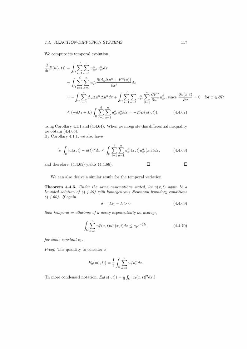
4.4. REACTION-DIFFUSION SYSTEMS 117
We compute its temporal evolution:
d
dtE(u(·, t)) =
∫
Ω
d∑
i=1
n∑
α=1
uαtxiuαxidx
=
∫
Ω
d∑
i=1
n∑
α=1
uαxi
∂(dα∆uα + Fα(u))
∂xidx
= −∫
Ω
n∑
α=1
dα∆uα∆uαdx+
∫
Ω
d∑
i=1
n∑
α=1
uαxi
n∑
β=1
∂Fα
∂uβuβxi , since
∂u(x, t)
∂ν= 0 for x ∈ ∂Ω
≤ (−dλ1 + L)
∫
Ω
d∑
i=1
n∑
α=1
uαxiuαxidx = −2δE(u(·, t)), (4.4.67)
using Corollary 4.1.1 and (4.4.64). When we integrate this differential inequalitywe obtain (4.4.65).By Corollary 4.1.1, we also have
λ1
∫
Ω
|u(x, t) − u(t)|2dx ≤∫
Ω
d∑
i=1
n∑
α=1
uαxi(x, t)uαxi(x, t)dx, (4.4.68)
and therefore, (4.4.65) yields (4.4.66).
We can also derive a similar result for the temporal variation
Theorem 4.4.5. Under the same assumptions stated, let u(x, t) again be abounded solution of (4.4.49) with homogeneous Neumann boundary conditions(4.4.60). If again
δ = dλ1 − L > 0 (4.4.69)
then temporal oscillations of u decay exponentially on average,
∫
Ω
n∑
α=1
uαt (x, t)uαt (x, t)dx ≤ c3e−2δt, (4.4.70)
for some constant c3.
Proof. The quantity to consider is
E0(u(·, t)) =1
2
∫
Ω
n∑
α=1
uαt uαt dx.
(In more condensed notation, E0(u(·, t)) = 12
∫
Ω|ut(x, t)|2dx.)
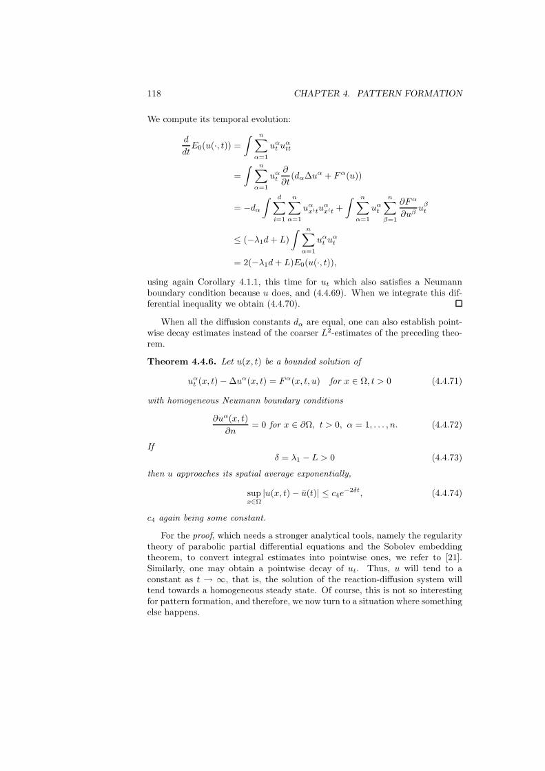
118 CHAPTER 4. PATTERN FORMATION
We compute its temporal evolution:
d
dtE0(u(·, t)) =
∫ n∑
α=1
uαt uαtt
=
∫ n∑
α=1
uαt∂
∂t(dα∆uα + Fα(u))
= −dα∫ d
∑
i=1
n∑
α=1
uαxituαxit +
∫ n∑
α=1
uαt
n∑
β=1
∂Fα
∂uβuβt
≤ (−λ1d+ L)
∫ n∑
α=1
uαt uαt
= 2(−λ1d+ L)E0(u(·, t)),
using again Corollary 4.1.1, this time for ut which also satisfies a Neumannboundary condition because u does, and (4.4.69). When we integrate this dif-ferential inequality we obtain (4.4.70).
When all the diffusion constants dα are equal, one can also establish point-wise decay estimates instead of the coarser L2-estimates of the preceding theo-rem.
Theorem 4.4.6. Let u(x, t) be a bounded solution of
uαt (x, t) − ∆uα(x, t) = Fα(x, t, u) for x ∈ Ω, t > 0 (4.4.71)
with homogeneous Neumann boundary conditions
∂uα(x, t)
∂n= 0 for x ∈ ∂Ω, t > 0, α = 1, . . . , n. (4.4.72)
Ifδ = λ1 − L > 0 (4.4.73)
then u approaches its spatial average exponentially,
supx∈Ω
|u(x, t) − u(t)| ≤ c4e−2δt, (4.4.74)
c4 again being some constant.
For the proof, which needs a stronger analytical tools, namely the regularitytheory of parabolic partial differential equations and the Sobolev embeddingtheorem, to convert integral estimates into pointwise ones, we refer to [21].Similarly, one may obtain a pointwise decay of ut. Thus, u will tend to aconstant as t → ∞, that is, the solution of the reaction-diffusion system willtend towards a homogeneous steady state. Of course, this is not so interestingfor pattern formation, and therefore, we now turn to a situation where somethingelse happens.
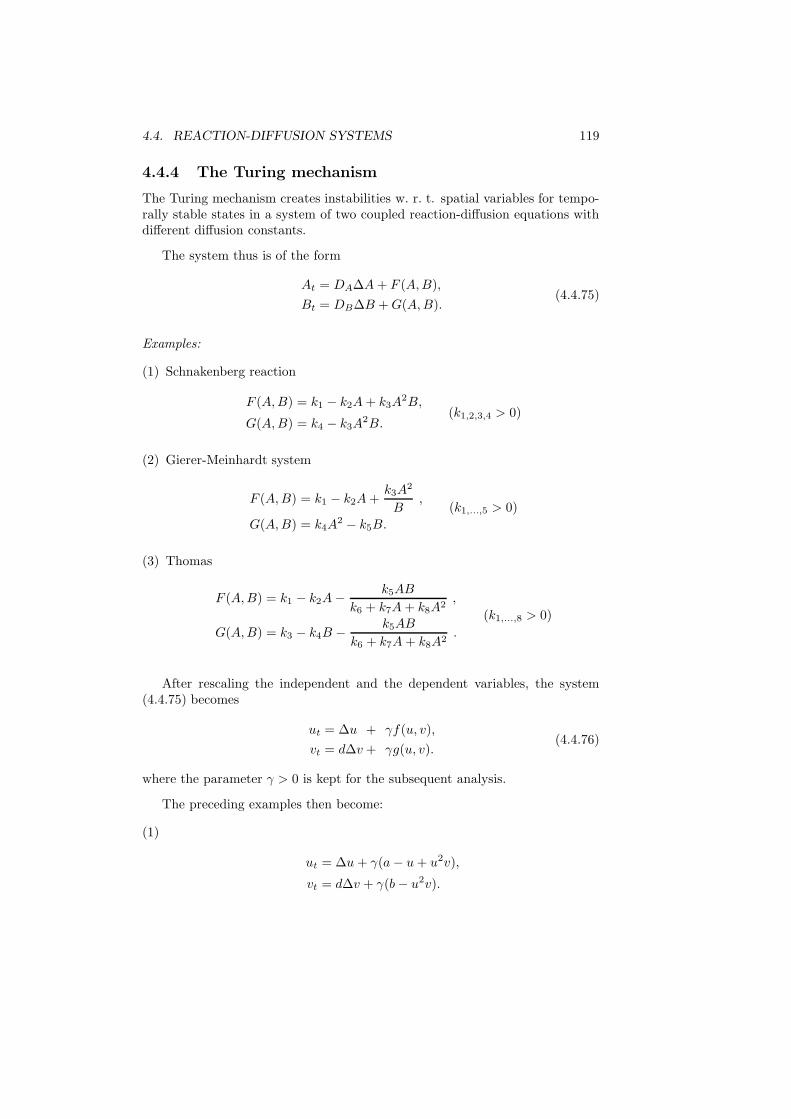
4.4. REACTION-DIFFUSION SYSTEMS 119
4.4.4 The Turing mechanism
The Turing mechanism creates instabilities w. r. t. spatial variables for tempo-rally stable states in a system of two coupled reaction-diffusion equations withdifferent diffusion constants.
The system thus is of the form
At = DA∆A+ F (A,B),
Bt = DB∆B +G(A,B).(4.4.75)
Examples:
(1) Schnakenberg reaction
F (A,B) = k1 − k2A+ k3A2B,
G(A,B) = k4 − k3A2B.
(k1,2,3,4 > 0)
(2) Gierer-Meinhardt system
F (A,B) = k1 − k2A+k3A
2
B,
G(A,B) = k4A2 − k5B.
(k1,...,5 > 0)
(3) Thomas
F (A,B) = k1 − k2A− k5AB
k6 + k7A+ k8A2,
G(A,B) = k3 − k4B − k5AB
k6 + k7A+ k8A2.
(k1,...,8 > 0)
After rescaling the independent and the dependent variables, the system(4.4.75) becomes
ut = ∆u + γf(u, v),
vt = d∆v + γg(u, v).(4.4.76)
where the parameter γ > 0 is kept for the subsequent analysis.
The preceding examples then become:
(1)
ut = ∆u + γ(a− u+ u2v),
vt = d∆v + γ(b− u2v).

120 CHAPTER 4. PATTERN FORMATION
(2)
ut = ∆u+ γ(a− bu+u2
v),
vt = d∆v + γ(u2 − v).
(3)
ut = ∆u+ γ(a− u− ρuv
1 + u+Ku2),
vt = d∆v + γ(α(b − v) − ρuv
1 + u+Ku2).
A slightly more general version of (2) is
(2’)
ut = ∆u+ γ(
a− u+u2
v(1 + ku2)
)
,
vt = d∆v + γ(u2 − v).
Here u, v : Ω×R+ → R for some bounded domain Ω ⊂ R
d, and we fix the initialvalues
u(x, 0), v(x, 0) for x ∈ Ω,
and impose Neumann boundary conditions
∂u
∂n(x, t) = 0 =
∂v
∂n(x, t) for all x ∈ ∂Ω, t ≥ 0.
(We have already seen in 4.4.1 that Neumann boundary conditions are welladapted for comparing the solutions of reaction-diffusion system with the onesof the underlying reaction system. – One can also study periodic boundary con-ditions, or, more generally, consider u, v as functions on some compact manifoldin place of the domain Ω.)
The mechanism starts with a fixed point (u⋆, v⋆) of the reaction system:
f(u⋆, v⋆) = 0 = g(u⋆, v⋆)
that is linearly stable. One then investigates its stability under spatially inho-mogeneous perturbations. According to the discussion following (4.3.164), thestability as a solution of the reaction system means that all eigenvalues λ of
A :=
(
fu(u⋆, v⋆) fv(u⋆, v⋆)gu(u⋆, vstar) gv(u⋆, v⋆)
)
(4.4.77)
have negative real part,Re(λ) < 0. (4.4.78)
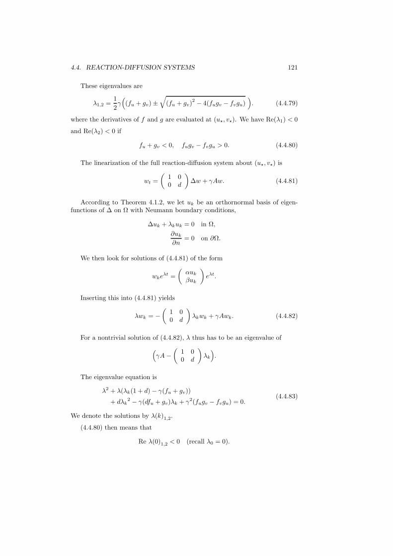
4.4. REACTION-DIFFUSION SYSTEMS 121
These eigenvalues are
λ1,2 =1
2γ(
(fu + gv) ±√
(fu + gv)2 − 4(fugv − fvgu)
)
. (4.4.79)
where the derivatives of f and g are evaluated at (u⋆, v⋆). We have Re(λ1) < 0
and Re(λ2) < 0 if
fu + gv < 0, fugv − fvgu > 0. (4.4.80)
The linearization of the full reaction-diffusion system about (u⋆, v⋆) is
wt =
(
1 00 d
)
∆w + γAw. (4.4.81)
According to Theorem 4.1.2, we let uk be an orthornormal basis of eigen-functions of ∆ on Ω with Neumann boundary conditions,
∆uk + λkuk = 0 in Ω,
∂uk∂n
= 0 on ∂Ω.
We then look for solutions of (4.4.81) of the form
wkeλt =
(
αukβuk
)
eλt.
Inserting this into (4.4.81) yields
λwk = −(
1 00 d
)
λkwk + γAwk. (4.4.82)
For a nontrivial solution of (4.4.82), λ thus has to be an eigenvalue of
(
γA−(
1 00 d
)
λk
)
.
The eigenvalue equation is
λ2 + λ(λk(1 + d) − γ(fu + gv))
+ dλk2 − γ(dfu + gv)λk + γ2(fugv − fvgu) = 0.
(4.4.83)
We denote the solutions by λ(k)1,2.
(4.4.80) then means that
Re λ(0)1,2 < 0 (recall λ0 = 0).
122 CHAPTER 4. PATTERN FORMATION
We now wish to investigate whether we can have
Re λ(k) > 0 (4.4.84)
for some higher mode λk.
Since by (4.4.80), λk > 0, d > 0, clearly
λk(1 + d) − γ(fu + gv) > 0,
we need for (4.4.84) that
dλk2 − γ(dfu + gv)λk + γ2(fugv − fvgu) < 0. (4.4.85)
Because of (4.4.80), this can only happen if
dfu + gv > 0.
Comparing this with the first equation of (4.4.80), we thus need
d > 1,
fugv < 0.
If we assume
fu > 0, gv < 0, (4.4.86)
then we need
d > 1. (4.4.87)
This is not enough to get (4.4.85) negative. In order to achieve this for somevalue of λk, we first determine that value µ of λk for which the lhs of (4.4.85)is minimized, i. e.
µ =γ
2d(dfu + gv), (4.4.88)
and we then need that the lhs of (4.4.85) becomes negative for λk = µ. This isequivalent to
(dfu + gv)2
4d> fugv − fvgu. (4.4.89)
If (4.4.89) holds, then the lhs of (4.4.85) has two values of λk where itvanishes, namely
µ± =γ
2d
(
(dfu + gv) ±√
(dfu + gv)2 − 4d(fugv − fvgu)
)
=γ
2d
(
(dfu + gv) ±√
(dfu − gv)2
+ 4dfvgu
)
(4.4.90)
4.4. REACTION-DIFFUSION SYSTEMS 123
and it becomes negative for
µ− < λk < µ+. (4.4.91)
We conclude
Lemma 4.4.2. Suppose (4.4.89) holds. Then (u⋆, v⋆) is spatially unstablew. r. t. the mode λk, i. e. there exists a solution of (4.4.82) with
Re λ > 0
if λk satisfies (4.4.91), where µ± are given by (4.4.90).
(4.4.89) is satisfied for
d > dc = −2fvgu − fugvf2u
+2
f2u
√
fvgu(fvgu − fugv) . (4.4.92)
Whether there exists an eigenvalue λk of ∆ satisfying (4.4.91) depends on thegeometry of Ω. In particular, according to the discussion after Theorem 4.1.2,the eigenvalues scale like ‖Ω‖− 2
d . Thus, if Ω is small, all nonzero eigenvaluesare large. Therefore, if Ω is sufficiently small, all nonzero eigenvalues are largerthan µ+.We can also keep Ω, and thus the smallest nonzero eigenvalue λ1, fixed andchoose γ > 0 in (4.4.90) so small that
µ+ < λ1.
Then, again, (4.4.91) cannot be solved. From these considerations we see thatwe need a certain minimal domain size for a given reaction strength, or else acertain minimal reaction strength for a given domain size, for a Turing instabilityto occur.
If the condition (4.4.91) is satisfied for some eigenvalue λk, it is also ofgeometric significance for which value of k this happens. Namely, by Courant’snodal domain theorem, the nodal set uk = 0 of the eigenfunction uk dividesΩ into at most (k+1) regions. On any of these regions, uk then has a fixed sign,i. e. is either positive or negative on that entire region. Since uk is the unstablemode, this controls the number of oscillations of the developing instability.
We summarize our considerations in
Theorem 4.4.7. Suppose that at a solution (u⋆, v⋆) of
f(u⋆, v⋆) = 0 = g(u⋆, v⋆),
we have
fu + gv < 0, fugv − fvgu > 0.
124 CHAPTER 4. PATTERN FORMATION
Then (u⋆, v⋆) is linearly stable for the reaction system
ut = γf(u, v),
vt = γg(u, v).
Suppose that d > 1 satisfiesdfu + gv > 0,
(dfu + gv)2 − 4d(fugv − fvgu) > 0.
Then (u⋆, v⋆) as a solution of the reaction-diffusion system
ut = ∆u + γf(u, v),
vt = d∆v + γg(u, v)
is linearly unstable against spatial oscillations with eigenvalue λk whenever λksatisfies (4.4.91).
Since the eigenvalues λk of ∆ on the bounded domain Ω are discrete (recallTheorem 4.1.2), it depends on the geometry of Ω whether such an eigenvalue inthe range determined by (4.4.91) exists. The number k controls the frequencyof oscillations of the instability about (u⋆, v⋆), and thus determines the shapeof the resulting spatial pattern.
Thus, in the situation described in Theorem 4.4.7, the equilibrium state(u⋆, v⋆) is unstable, and in the vicinity of it, perturbations grow at a rate eReλ,where λ solves (4.4.83).
Typically, one assumes, however, that the dynamics is confined within abounded region in (R+)
2. This means that appropriate assumptions on f and
g for u = 0 or v = 0, or for u and v large ensure that solutions starting in thepositive quadrant can neither become zero nor unbounded. In 4.4.3 we havediscussed the principle that if such a confinement holds for the reaction system,it also holds for the reaction-diffusion system.
Thus, even though (u⋆, v⋆) is locally unstable, and therefore small pertur-bations grow exponentially, this growth has to terminate eventually, and oneexpects that the corresponding solution of the reaction-diffusion system settlesat a spatially inhomogeneous steady state. This is the idea of the Turing mech-anism. This has not yet been demonstrated in full rigour and generality. Sofar, the existence of spatially heterogeneous solutions has only been shown bysingular perturbation analysis near the critical parameter dc in (4.4.92).We should also point out that Turing structures show that what we have dis-cussed at the end of 4.4.3, namely that solutions of reaction-diffusion systemsbecome spatially homogeneous as time tends to infinity, is by no means a univer-sal phenomenon, but rather depends on specific assumptions. Clearly, spatiallyinhomogeneous structures as produced by the Turing mechanism are more in-teresting for pattern formation than homogeneous ones. Of course, the situationbecomes even richer when the asymptotic structures are not only not spatially
4.4. REACTION-DIFFUSION SYSTEMS 125
homogeneous, but also not steady in time. For example, a Turing instabilitycould get combined with a Hopf bifurcation. See [37] for examples.
With Theorem 4.4.7, we return to example (1) above. We have
u⋆ = a+ b,
v⋆ =b
(a+ b)2 ,
(of course, a, b > 0)
and at (u⋆, v⋆) then
fu =b− a
a+ b,
fv = (a+ b)2,
gu = − 2b
a+ b,
gv = −(a+ b)2,
fugv − fvgu = (a+ b)2> 0.
Since we need that fu and gv have opposite signs (in order to get dfu+gv > 0later on), we require
b > a.
fu + gv < 0 then imples
0 < b− a < (a+ b)3, (4.4.93)
while dfu + gv > 0 implies
d(b − a) > (a+ b)3. (4.4.94)
Finally, (dfu + gv)2 − 4d(fugv − fvgu) > 0 requires
(
d(b− a) − (a+ b)3)2
> 4d(a+ b)4. (4.4.95)
The Turing mechanism is a beautiful analytical scheme for pattern forma-tion. This, however, does not imply that this really is the general scheme under-lying the formation of spatial patterns in biology. In fact, according to recentdevelopments in developmental biology, the combinatorial patterns of gene reg-ulation constitute the basic mechanism for the formation of spatial structures,rather than the Turing mechanism. Nevertheless, in certain cases, Turing’s idea[36] may apply. Many examples are discussed in [28].The present section follows the presentation in [21] rather closely.
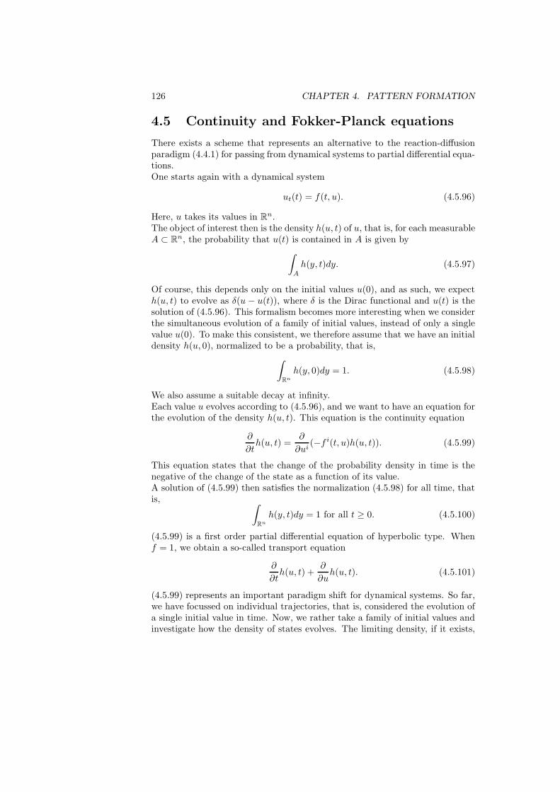
126 CHAPTER 4. PATTERN FORMATION
4.5 Continuity and Fokker-Planck equations
There exists a scheme that represents an alternative to the reaction-diffusionparadigm (4.4.1) for passing from dynamical systems to partial differential equa-tions.One starts again with a dynamical system
ut(t) = f(t, u). (4.5.96)
Here, u takes its values in Rn.
The object of interest then is the density h(u, t) of u, that is, for each measurableA ⊂ R
n, the probability that u(t) is contained in A is given by
∫
A
h(y, t)dy. (4.5.97)
Of course, this depends only on the initial values u(0), and as such, we expecth(u, t) to evolve as δ(u − u(t)), where δ is the Dirac functional and u(t) is thesolution of (4.5.96). This formalism becomes more interesting when we considerthe simultaneous evolution of a family of initial values, instead of only a singlevalue u(0). To make this consistent, we therefore assume that we have an initialdensity h(u, 0), normalized to be a probability, that is,
∫
Rn
h(y, 0)dy = 1. (4.5.98)
We also assume a suitable decay at infinity.Each value u evolves according to (4.5.96), and we want to have an equation forthe evolution of the density h(u, t). This equation is the continuity equation
∂
∂th(u, t) =
∂
∂ui(−f i(t, u)h(u, t)). (4.5.99)
This equation states that the change of the probability density in time is thenegative of the change of the state as a function of its value.A solution of (4.5.99) then satisfies the normalization (4.5.98) for all time, thatis,
∫
Rn
h(y, t)dy = 1 for all t ≥ 0. (4.5.100)
(4.5.99) is a first order partial differential equation of hyperbolic type. Whenf = 1, we obtain a so-called transport equation
∂
∂th(u, t) +
∂
∂uh(u, t). (4.5.101)
(4.5.99) represents an important paradigm shift for dynamical systems. So far,we have focussed on individual trajectories, that is, considered the evolution ofa single initial value in time. Now, we rather take a family of initial values andinvestigate how the density of states evolves. The limiting density, if it exists,
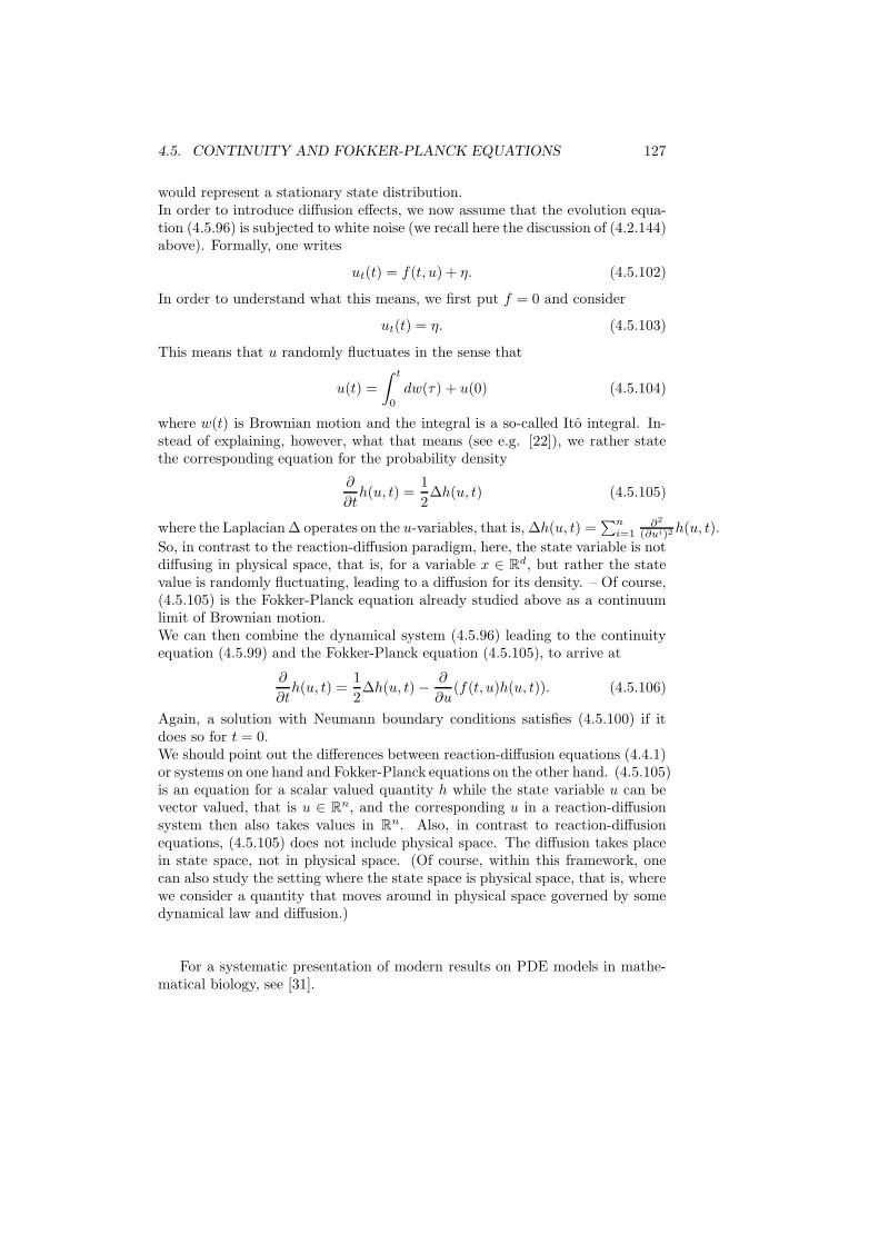
4.5. CONTINUITY AND FOKKER-PLANCK EQUATIONS 127
would represent a stationary state distribution.In order to introduce diffusion effects, we now assume that the evolution equa-tion (4.5.96) is subjected to white noise (we recall here the discussion of (4.2.144)above). Formally, one writes
ut(t) = f(t, u) + η. (4.5.102)
In order to understand what this means, we first put f = 0 and consider
ut(t) = η. (4.5.103)
This means that u randomly fluctuates in the sense that
u(t) =
∫ t
0
dw(τ) + u(0) (4.5.104)
where w(t) is Brownian motion and the integral is a so-called Ito integral. In-stead of explaining, however, what that means (see e.g. [22]), we rather statethe corresponding equation for the probability density
∂
∂th(u, t) =
1
2∆h(u, t) (4.5.105)
where the Laplacian ∆ operates on the u-variables, that is, ∆h(u, t) =∑ni=1
∂2
(∂ui)2 h(u, t).
So, in contrast to the reaction-diffusion paradigm, here, the state variable is notdiffusing in physical space, that is, for a variable x ∈ R
d, but rather the statevalue is randomly fluctuating, leading to a diffusion for its density. – Of course,(4.5.105) is the Fokker-Planck equation already studied above as a continuumlimit of Brownian motion.We can then combine the dynamical system (4.5.96) leading to the continuityequation (4.5.99) and the Fokker-Planck equation (4.5.105), to arrive at
∂
∂th(u, t) =
1
2∆h(u, t) − ∂
∂u(f(t, u)h(u, t)). (4.5.106)
Again, a solution with Neumann boundary conditions satisfies (4.5.100) if itdoes so for t = 0.We should point out the differences between reaction-diffusion equations (4.4.1)or systems on one hand and Fokker-Planck equations on the other hand. (4.5.105)is an equation for a scalar valued quantity h while the state variable u can bevector valued, that is u ∈ R
n, and the corresponding u in a reaction-diffusionsystem then also takes values in R
n. Also, in contrast to reaction-diffusionequations, (4.5.105) does not include physical space. The diffusion takes placein state space, not in physical space. (Of course, within this framework, onecan also study the setting where the state space is physical space, that is, wherewe consider a quantity that moves around in physical space governed by somedynamical law and diffusion.)
For a systematic presentation of modern results on PDE models in mathe-matical biology, see [31].

128 CHAPTER 4. PATTERN FORMATION
Thanks for discussions to Ugur Abdullah, Anirban Banerjee, Andreas Dress,Benoıt Perthame, Angela Stevens
Bibliography
[1] H.-J. Bandelt, A.Dress, A canonical decomposition theory for metrics ona finite set, Adv.Math.92, 47-105, 1992
[2] E.Bender, E.Canfield, The asymptotic number of labeled graphs withgiven degree sequences, J.Comb.Th.A 24, 296-307, 1978
[3] B.Bolobas, Random graphs, Cambridge Univ.Press, 22001
[4] B.Bolobas, Modern graph theory, Springer, 1998
[5] F.Chung, Spectral graph theory, AMS, 1997
[6] H.Colonius, H.Schulze, Tree structures for proximity data,Brit.J.Math.Statist.Psychol.34, 167-180, 1981
[7] R.Courant, K.Friedrichs, H.Lewy, Uber die partiellen Differentialgleichun-gen der mathematischen Physik, Math.Ann.100, 32-74, 1928
[8] P.Dayan, L.F.Abbott, Theoretical Neuroscience, MIT Press, 2001
[9] A.Dress, Recent results and new problems in phylogenetic combinatorics
[10] P.Erdos, A.Renyi, On random graphs.I, Publ.Math.Debrecen 6, 290-291,1959
[11] L.C.Evans, Partial differential equations, AMS, 1998
[12] W.Ewens, Mathematical population genetics, I. Theoretical introduction,Springer, 22004
[13] G.Gladwell, E.Davies, J.Leydold, and P.Stadler, Discrete nodal domaintheorems, Lin.Alg.Appl.336, 2001, 51-60
[14] C.Godsil, G.Royle, Algebraic graph theory, Springer, 2001
[15] G.Grimmett, D.Stirzacker, Probability and random processes, OxfordUniv.Press, 32001
[16] P.Haccou, P.Jagers, V.A.Vatutin, Branching processes, CambridgeUniv.Press, 2005
129
130 BIBLIOGRAPHY
[17] J.Hein, M.Schierup. C.Wiuf, Gene genealogies, variation and evolution,Oxford Univ.Press, 2005
[18] W.Hennig, Phylogenetische Systematik, Paul Parey, Berlin and Hamburg,1982
[19] J.Hofbauer, K.Sigmund, The theory of evolution and dynamical systems,Cambridge Univ. Press, 1988
[20] J.Hofbauer, K.Sigmund, Evolutionary games and population dynamics,Cambridge Univ. Press, 1998
[21] J.Jost, Partial differential equations, Springer, 22007
[22] J.Jost, Dynamical systems, Springer, 2005
[23] M.Kimmel, D.Axelrod, Branching processes in biology, Springer, 2002
[24] E.Klipp, R.Herwig, A.Kowald, C.Wierling, H.Lehrach, Systems biology inpractice, Wiley-VCH, 2005
[25] C.Koch, Biophysics of computation, Oxford Univ.Press, New York, 1999
[26] A.Kolmogoroff, I.Petrovsky, N.Piscounoff, Etude de l’ equation de la dif-fusion avec croissance de la quantite de la matiere et son application a unprobleme biologique, Moscow Univ.Bull.Math.1, 1937, 1-25
[27] A.Lasota, M.Mackey, Chaos, fractals, and noise, Springer, 21994
[28] J.Murray, Mathematical biology, Springer, 1989
[29] M.Newman, Random graphs as models of networks, in: S.Bornholdt,H.G.Schuster (eds.), Handbook of graphs and networks, Wiley-VCH,Berlin, 2002
[30] B.Øksendal, Stochastic differential equations, Springer, 41995
[31] B.Perthame, Transport equations in biology, Birkhauser, 2007
[32] P.Phillipson, P.Schuster, An analytical picture of neuron oscillations,Int.J.Bifurc.Chaos 14, 1539-1548, 2004
[33] C.Semple, M.Steel, Phylogenetics, Oxford Univ.Press, 2003
[34] J.Smoller, Shock waves and reaction-diffusion equations, Springer, 1983
[35] K.Strimmer, A. von Haeseler, Quartet puzzling: a quartet maximum likeli-hood method for reconstructing tree topologies, Mol.BiolEvol.13, 964-996,1996
[36] A.Turing
[37] Walgraef