Inside Oracle Database 10g

Oracle Database 10g: The Top 20 Features for DBAsby Arup Nanda

Over the last 27 years, Oracle has made tremendous improvements in its core database product. Now, that product is not only the world's most reliable and performant database, but also part of a complete software infrastructure for enterprise computing. With each new release comes a sometimes dizzying display of new capabilities and features, sometimes leaving developers, IT managers, and even seasoned DBAs wondering which new features will benefit them most.

With the introduction of Oracle Database 10g, DBAs will have in their hands one of the most profound new releases ever from Oracle. So, DBAs who take the time to understand the proper application of new Oracle technology to their everyday jobs will enjoy many time-saving, and ultimately, money-saving new capabilities.

Oracle Database 10g offers many new tools that help DBAs work more efficiently (and perhaps more enjoyably), freeing them for more strategic, creative endeavors—not to mention their nights and weekends. Oracle Database 10g really is that big of a deal for DBAs.

Over the new 20 weeks, I will help you through the ins and outs of this powerful new release by presenting what I consider to be the top 20 new Oracle Database 10g features for database administration tasks. This list ranges from the rudimentary, such as setting a default tablespace for creating users, to the advanced, such as the new Automatic Storage Management feature.

In this series, I will provide brief, focused analyses of these interesting new tools and techniques. The goal is to outline the functions and benefits of the feature so that you can put it into action in your environment as quickly as possible.

I welcome your thoughts, comments, and questions about this series. Enjoy!

Schedule Week 1—Flashback Versions QueryWeek 2—Rollback MonitoringWeek 3—Tablespace ManagementWeek 4—Oracle Data PumpWeek 5—Flashback TableWeek 6—Automatic Workload RepositoryWeek 7—SQL*Plus Rel 10.1Week 8—Automatic Storage ManagementWeek 9—RMANWeek 10—Auditing

Week 11—Wait InterfaceWeek 12—Materialized ViewsWeek 13—Enterprise Manager 10gWeek 14—Virtual Private DatabaseWeek 15—Automatic Segment ManagementWeek 16—Transportable TablespacesWeek 17—Automatic Shared Memory ManagementWeek 18—ADDM and SQL Tuning AdvisorWeek 19—SchedulerWeek 20—Best of the Rest

Release 2 Features Addendum New!

Week 1Get a Movie, Not a Picture: Flashback Versions Query

Immediately identify all the changes to a row, with zero setup required.

In Oracle9i Database, we saw the introduction of the "time machine" manifested in the form of Flashback Query. The feature allows the DBA to see the value of a column as of a specific time, as long as the before-image copy of the block is available in the undo segment. However, Flashback Query only provides a fixed snapshot of the data as of a time, not a running representation of changed data between two time points. Some applications, such as those involving the management of foreign currency, may need to see the value data changes in a period, not just at two points of time. Thanks to the Flashback Versions Query feature, Oracle Database 10g can perform that task easily and efficiently.

Querying Changes to a Table

In this example, I have used a bank's foreign currency management application. The database has a table called RATES to record exchange rate on specific times.

SQL> desc rates Name Null? Type ----------------- -------- ------------ CURRENCY VARCHAR2(4) RATE NUMBER(15,10)

This table shows the exchange rate of US$ against various other currencies as shown in the CURRENCY column. In the financial services industry, exchange rates are not merely updated when changed; rather, they are recorded in a history. This approach is required because bank transactions can occur as applicable to a "past time," to accommodate the loss in time because of remittances. For example, for a transaction that occurs at 10:12AM but is effective as of 9:12AM, the applicable rate is that at 9:12AM, not now.

Up until now, the only option was to create a rate history table to store the rate changes, and then query that table to see if a history is available. Another option was to record the start and end times of the applicability of the particular exchange rate in the RATES table itself. When the change occurred, the END_TIME column in the existing row was updated to SYSDATE and a new row was inserted with the new rate with the END_TIME as NULL.

In Oracle Database 10g, however, the Flashback Versions Query feature may obviate the need to maintain a history table or store start and end times. Rather, using this feature, you can get the value of a row as of a specific time in the past with no additional setup. Bear in mind, however, that it depends on the availability of the undo information in the database, so if the undo information has been aged out, this approach will fail.

For example, say that the DBA, in the course of normal business, updates the rate several times—or even deletes a row and reinserts it:

insert into rates values ('EURO',1.1012);commit;update rates set rate = 1.1014;commit;update rates set rate = 1.1013;commit;delete rates;commit;insert into rates values ('EURO',1.1016);commit;update rates set rate = 1.1011;commit;

After this set of activities, the DBA would get the current committed value of RATE column by

SQL> select * from rates;

CURR RATE---- ----------EURO 1.1011

This output shows the current value of the RATE, not all the changes that have occurred since the first time the row was created. Thus using Flashback Query, you can find out the value at a given point in time; but we are more interested in building an audit trail of the changes—somewhat like recording changes through a camcorder, not just as a series of snapshots taken at a certain point.

The following query shows the changes made to the table:

select versions_starttime, versions_endtime, versions_xid, versions_operation, rate from rates versions between timestamp minvalue and maxvalueorder by VERSIONS_STARTTIME/

VERSIONS_STARTTIME VERSIONS_ENDTIME VERSIONS_XID V RATE---------------------- ---------------------- ---------------- - ----------01-DEC-03 03.57.12 PM 01-DEC-03 03.57.30 PM 0002002800000C61 I 1.1012

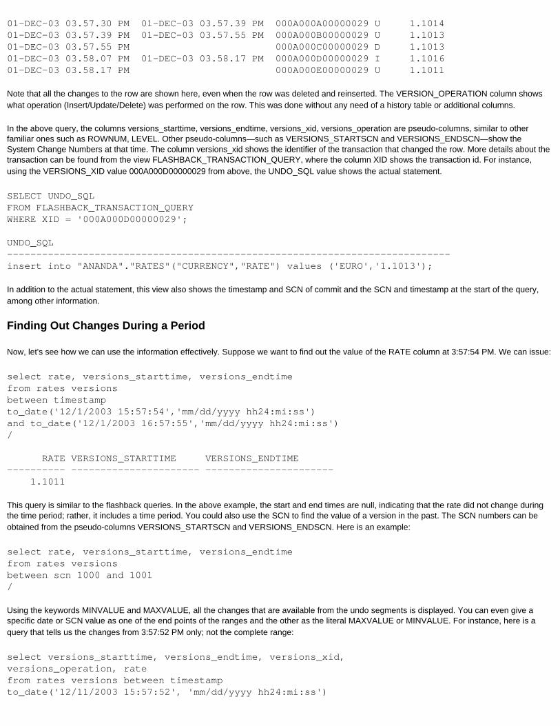
01-DEC-03 03.57.30 PM 01-DEC-03 03.57.39 PM 000A000A00000029 U 1.101401-DEC-03 03.57.39 PM 01-DEC-03 03.57.55 PM 000A000B00000029 U 1.101301-DEC-03 03.57.55 PM 000A000C00000029 D 1.101301-DEC-03 03.58.07 PM 01-DEC-03 03.58.17 PM 000A000D00000029 I 1.101601-DEC-03 03.58.17 PM 000A000E00000029 U 1.1011

Note that all the changes to the row are shown here, even when the row was deleted and reinserted. The VERSION_OPERATION column shows what operation (Insert/Update/Delete) was performed on the row. This was done without any need of a history table or additional columns.

In the above query, the columns versions_starttime, versions_endtime, versions_xid, versions_operation are pseudo-columns, similar to other familiar ones such as ROWNUM, LEVEL. Other pseudo-columns—such as VERSIONS_STARTSCN and VERSIONS_ENDSCN—show the System Change Numbers at that time. The column versions_xid shows the identifier of the transaction that changed the row. More details about the transaction can be found from the view FLASHBACK_TRANSACTION_QUERY, where the column XID shows the transaction id. For instance, using the VERSIONS_XID value 000A000D00000029 from above, the UNDO_SQL value shows the actual statement.

SELECT UNDO_SQLFROM FLASHBACK_TRANSACTION_QUERYWHERE XID = '000A000D00000029';

UNDO_SQL----------------------------------------------------------------------------insert into "ANANDA"."RATES"("CURRENCY","RATE") values ('EURO','1.1013');

In addition to the actual statement, this view also shows the timestamp and SCN of commit and the SCN and timestamp at the start of the query, among other information.

Finding Out Changes During a Period

Now, let's see how we can use the information effectively. Suppose we want to find out the value of the RATE column at 3:57:54 PM. We can issue:

select rate, versions_starttime, versions_endtimefrom rates versionsbetween timestamp to_date('12/1/2003 15:57:54','mm/dd/yyyy hh24:mi:ss')and to_date('12/1/2003 16:57:55','mm/dd/yyyy hh24:mi:ss')/

RATE VERSIONS_STARTTIME VERSIONS_ENDTIME---------- ---------------------- ---------------------- 1.1011

This query is similar to the flashback queries. In the above example, the start and end times are null, indicating that the rate did not change during the time period; rather, it includes a time period. You could also use the SCN to find the value of a version in the past. The SCN numbers can be obtained from the pseudo-columns VERSIONS_STARTSCN and VERSIONS_ENDSCN. Here is an example:

select rate, versions_starttime, versions_endtimefrom rates versionsbetween scn 1000 and 1001/

Using the keywords MINVALUE and MAXVALUE, all the changes that are available from the undo segments is displayed. You can even give a specific date or SCN value as one of the end points of the ranges and the other as the literal MAXVALUE or MINVALUE. For instance, here is a query that tells us the changes from 3:57:52 PM only; not the complete range:

select versions_starttime, versions_endtime, versions_xid, versions_operation, rate from rates versions between timestamp to_date('12/11/2003 15:57:52', 'mm/dd/yyyy hh24:mi:ss')

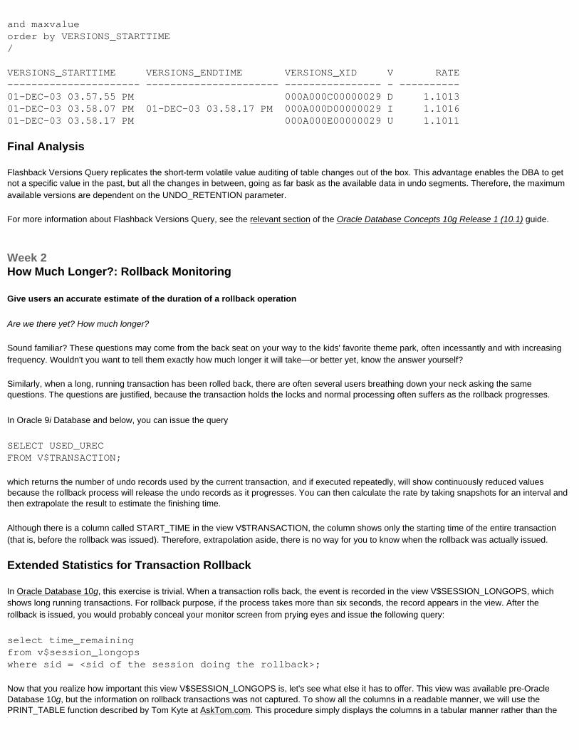
and maxvalueorder by VERSIONS_STARTTIME/

VERSIONS_STARTTIME VERSIONS_ENDTIME VERSIONS_XID V RATE---------------------- ---------------------- ---------------- - ----------01-DEC-03 03.57.55 PM 000A000C00000029 D 1.101301-DEC-03 03.58.07 PM 01-DEC-03 03.58.17 PM 000A000D00000029 I 1.101601-DEC-03 03.58.17 PM 000A000E00000029 U 1.1011

Final Analysis

Flashback Versions Query replicates the short-term volatile value auditing of table changes out of the box. This advantage enables the DBA to get not a specific value in the past, but all the changes in between, going as far bask as the available data in undo segments. Therefore, the maximum available versions are dependent on the UNDO_RETENTION parameter.

For more information about Flashback Versions Query, see the relevant section of the Oracle Database Concepts 10g Release 1 (10.1) guide.

Week 2How Much Longer?: Rollback Monitoring

Give users an accurate estimate of the duration of a rollback operation

Are we there yet? How much longer?

Sound familiar? These questions may come from the back seat on your way to the kids' favorite theme park, often incessantly and with increasing frequency. Wouldn't you want to tell them exactly how much longer it will take—or better yet, know the answer yourself?

Similarly, when a long, running transaction has been rolled back, there are often several users breathing down your neck asking the same questions. The questions are justified, because the transaction holds the locks and normal processing often suffers as the rollback progresses.

In Oracle 9i Database and below, you can issue the query

SELECT USED_URECFROM V$TRANSACTION;

which returns the number of undo records used by the current transaction, and if executed repeatedly, will show continuously reduced values because the rollback process will release the undo records as it progresses. You can then calculate the rate by taking snapshots for an interval and then extrapolate the result to estimate the finishing time.

Although there is a column called START_TIME in the view V$TRANSACTION, the column shows only the starting time of the entire transaction (that is, before the rollback was issued). Therefore, extrapolation aside, there is no way for you to know when the rollback was actually issued.

Extended Statistics for Transaction Rollback

In Oracle Database 10g, this exercise is trivial. When a transaction rolls back, the event is recorded in the view V$SESSION_LONGOPS, which shows long running transactions. For rollback purpose, if the process takes more than six seconds, the record appears in the view. After the rollback is issued, you would probably conceal your monitor screen from prying eyes and issue the following query:

select time_remainingfrom v$session_longopswhere sid = <sid of the session doing the rollback>;

Now that you realize how important this view V$SESSION_LONGOPS is, let's see what else it has to offer. This view was available pre-Oracle Database 10g, but the information on rollback transactions was not captured. To show all the columns in a readable manner, we will use the PRINT_TABLE function described by Tom Kyte at AskTom.com. This procedure simply displays the columns in a tabular manner rather than the

usual line manner.

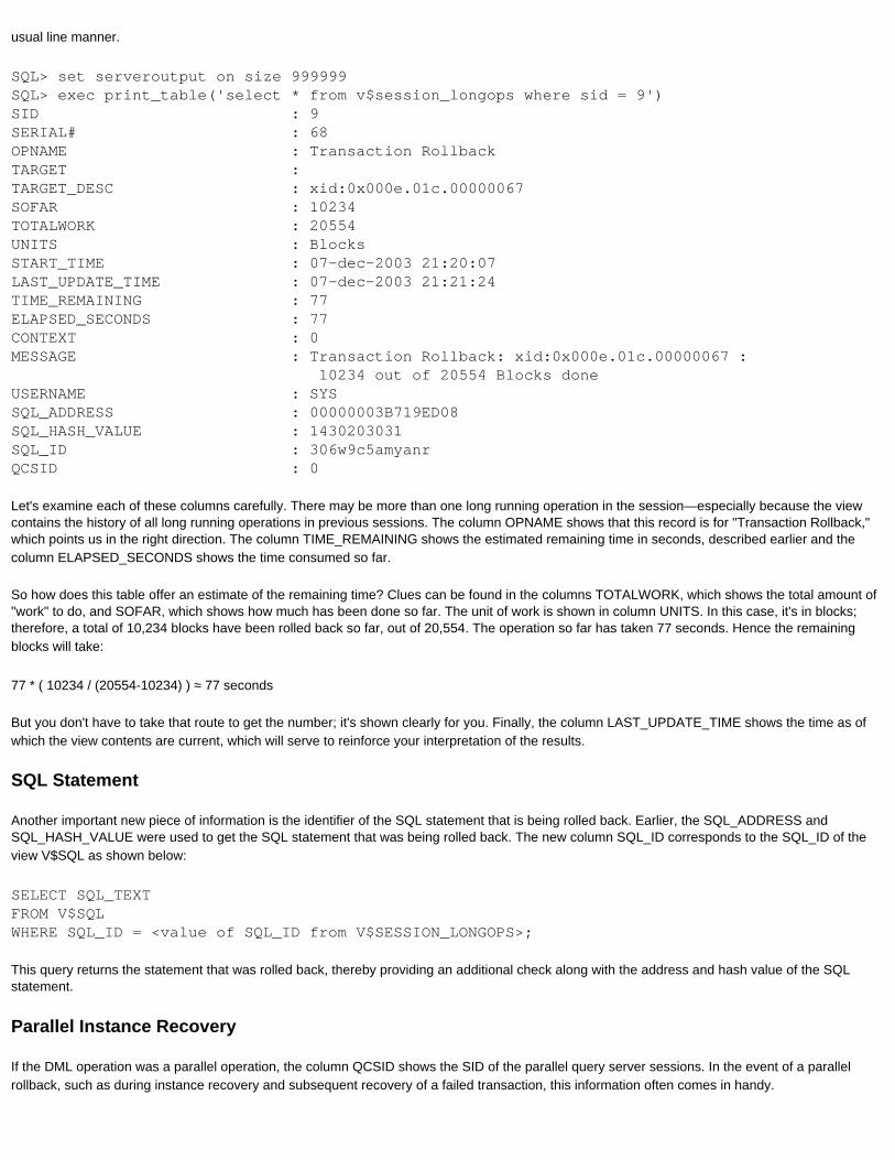
SQL> set serveroutput on size 999999SQL> exec print_table('select * from v$session_longops where sid = 9')SID : 9SERIAL# : 68OPNAME : Transaction RollbackTARGET :TARGET_DESC : xid:0x000e.01c.00000067SOFAR : 10234TOTALWORK : 20554UNITS : BlocksSTART_TIME : 07-dec-2003 21:20:07LAST_UPDATE_TIME : 07-dec-2003 21:21:24TIME_REMAINING : 77ELAPSED_SECONDS : 77CONTEXT : 0MESSAGE : Transaction Rollback: xid:0x000e.01c.00000067 : 10234 out of 20554 Blocks doneUSERNAME : SYSSQL_ADDRESS : 00000003B719ED08SQL_HASH_VALUE : 1430203031SQL_ID : 306w9c5amyanrQCSID : 0

Let's examine each of these columns carefully. There may be more than one long running operation in the session—especially because the view contains the history of all long running operations in previous sessions. The column OPNAME shows that this record is for "Transaction Rollback," which points us in the right direction. The column TIME_REMAINING shows the estimated remaining time in seconds, described earlier and the column ELAPSED_SECONDS shows the time consumed so far.

So how does this table offer an estimate of the remaining time? Clues can be found in the columns TOTALWORK, which shows the total amount of "work" to do, and SOFAR, which shows how much has been done so far. The unit of work is shown in column UNITS. In this case, it's in blocks; therefore, a total of 10,234 blocks have been rolled back so far, out of 20,554. The operation so far has taken 77 seconds. Hence the remaining blocks will take:

77 * ( 10234 / (20554-10234) ) ≈ 77 seconds

But you don't have to take that route to get the number; it's shown clearly for you. Finally, the column LAST_UPDATE_TIME shows the time as of which the view contents are current, which will serve to reinforce your interpretation of the results.

SQL Statement

Another important new piece of information is the identifier of the SQL statement that is being rolled back. Earlier, the SQL_ADDRESS and SQL_HASH_VALUE were used to get the SQL statement that was being rolled back. The new column SQL_ID corresponds to the SQL_ID of the view V$SQL as shown below:

SELECT SQL_TEXTFROM V$SQLWHERE SQL_ID = <value of SQL_ID from V$SESSION_LONGOPS>;

This query returns the statement that was rolled back, thereby providing an additional check along with the address and hash value of the SQL statement.

Parallel Instance Recovery

If the DML operation was a parallel operation, the column QCSID shows the SID of the parallel query server sessions. In the event of a parallel rollback, such as during instance recovery and subsequent recovery of a failed transaction, this information often comes in handy.

For example, suppose that during a large update the instance shuts down abnormally. When the instance comes up, the failed transaction is rolled back. If the value of the initialization parameter for parallel recovery is enabled, the rollback occurs in parallel instead of serially, as it occurs in regular transaction rollback. The next task is to estimate the completion time of the rollback process.

The view V$FAST_START_TRANSACTIONS shows the transaction(s) occurring to roll-back the failed ones. A similar view, V$FAST_START_SERVERS, shows the number of parallel query servers working on the rollback. These two views were available in previous versions, but the new column XID, which indicates transaction identifier, makes the joining easier. In Oracle9i Database and below, you would have had to join the views on three columns (USN - Undo Segment Number, SLT - the Slot Number within the Undo Segment, and SEQ - the sequence number). The parent sets were shown in PARENTUSN, PARENTSLT, and PARENTSEQ. In Oracle Database 10g, you only need to join it on the XID column and the parent XID is indicated by an intuitive name: PXID.

The most useful piece of information comes from the column RCVSERVERS in V$FAST_START_TRANSACTIONS view. If parallel rollback is going on, the number of parallel query servers is indicated in this column. You could check it to see how many parallel query processes started:

select rcvservers from v$fast_start_transactions;

If the output shows just 1, then the transaction is being rolled back serially by SMON process--obviously an inefficient way to do that. You can modify the initialization parameter RECOVERY_PARALLELISM to value other than 0 and 1 and restart the instance for a parallel rollback. You can then issue ALTER SYSTEM SET FAST_START_PARALLEL_ROLLBACK = HIGH to create parallel servers as much as 4 times the number of CPUs.

If the output of the above query shows anything other than 1, then parallel rollback is occurring. You can query the same view (V$FAST_START_TRANSACTIONS) to get the parent and child transactions (parent transaction id - PXID, and child - XID). The XID can also be used to join this view with V$FAST_START_SERVERS to get additional details.

Conclusion

In summary, when a long-running transaction is rolling back in Oracle Database 10g—be it the parallel instance recovery sessions or a user issued rollback statement—all you have to do is to look at the view V$SESSION_LONGOPS and estimate to a resolution of a second how much longer it will take.

Now if only it could predict the arrival time at the theme park!

Week 3What's in a Name?: Improved Tablespace Management

Tablespace management gets a boost thanks to a sparser SYSTEM, support for defining a default tablespace for users, new SYSAUX, and even renaming

How many times you have pulled your hair out in frustration over users creating segments other than SYS and SYSTEM in the SYSTEM tablespace?

Prior to Oracle9i Database, if the DEFAULT TABLESPACE was not specified when the user was created, it would default to the SYSTEM tablespace. If the user did not specify a tablespace explicitly while creating a segment, it was created in SYSTEM—provided the user had quota there, either explicitly granted or through the system privilege UNLIMITED TABLESPACE. Oracle9i alleviated this problem by allowing the DBA to specify a default, temporary tablespace for all users created without an explicit temporary tablespace clause.

In Oracle Database 10g, you can similarly specify a default tablespace for users. During database creation, the CREATE DATABASE command can contain the clause DEFAULT TABLESPACE <tsname>. After creation, you can make a tablespace the default by issuing

ALTER DATABASE DEFAULT TABLESPACE <tsname>;

All users created without the DEFAULT TABLESPACE clause will have <tsname> as their default. You can change the default tablespace at any time through this ALTER command, which allows you to specify different tablespaces as default at different points.

Important note: the default tablespaces of all users with the old tablespace are changed to <tsname>, even if something else was specified explicitly for some users. For instance, assume the default tablespaces for users USER1 and USER2 are TS1 and TS2 respectively, specified

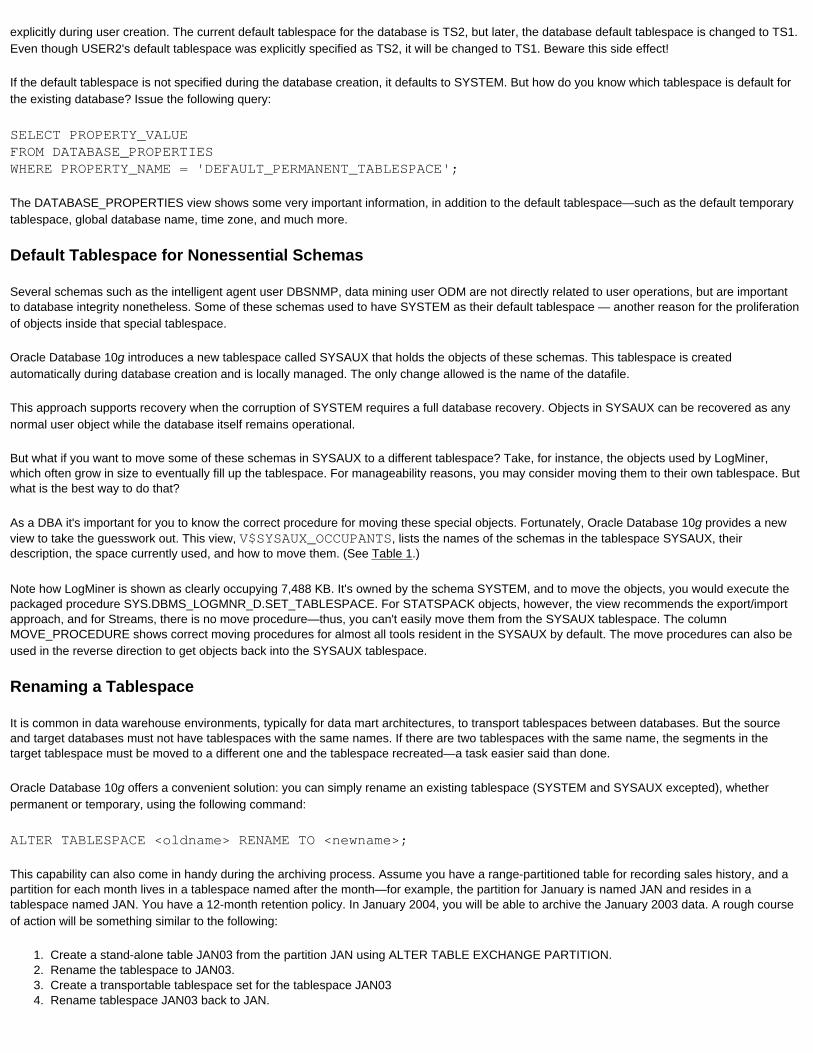
explicitly during user creation. The current default tablespace for the database is TS2, but later, the database default tablespace is changed to TS1. Even though USER2's default tablespace was explicitly specified as TS2, it will be changed to TS1. Beware this side effect!

If the default tablespace is not specified during the database creation, it defaults to SYSTEM. But how do you know which tablespace is default for the existing database? Issue the following query:

SELECT PROPERTY_VALUEFROM DATABASE_PROPERTIESWHERE PROPERTY_NAME = 'DEFAULT_PERMANENT_TABLESPACE';

The DATABASE_PROPERTIES view shows some very important information, in addition to the default tablespace—such as the default temporary tablespace, global database name, time zone, and much more.

Default Tablespace for Nonessential Schemas

Several schemas such as the intelligent agent user DBSNMP, data mining user ODM are not directly related to user operations, but are important to database integrity nonetheless. Some of these schemas used to have SYSTEM as their default tablespace — another reason for the proliferation of objects inside that special tablespace.

Oracle Database 10g introduces a new tablespace called SYSAUX that holds the objects of these schemas. This tablespace is created automatically during database creation and is locally managed. The only change allowed is the name of the datafile.

This approach supports recovery when the corruption of SYSTEM requires a full database recovery. Objects in SYSAUX can be recovered as any normal user object while the database itself remains operational.

But what if you want to move some of these schemas in SYSAUX to a different tablespace? Take, for instance, the objects used by LogMiner, which often grow in size to eventually fill up the tablespace. For manageability reasons, you may consider moving them to their own tablespace. But what is the best way to do that?

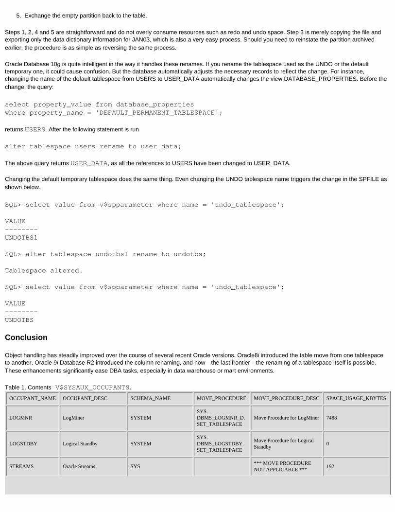
As a DBA it's important for you to know the correct procedure for moving these special objects. Fortunately, Oracle Database 10g provides a new view to take the guesswork out. This view, V$SYSAUX_OCCUPANTS, lists the names of the schemas in the tablespace SYSAUX, their description, the space currently used, and how to move them. (See Table 1.)

Note how LogMiner is shown as clearly occupying 7,488 KB. It's owned by the schema SYSTEM, and to move the objects, you would execute the packaged procedure SYS.DBMS_LOGMNR_D.SET_TABLESPACE. For STATSPACK objects, however, the view recommends the export/import approach, and for Streams, there is no move procedure—thus, you can't easily move them from the SYSAUX tablespace. The column MOVE_PROCEDURE shows correct moving procedures for almost all tools resident in the SYSAUX by default. The move procedures can also be used in the reverse direction to get objects back into the SYSAUX tablespace.

Renaming a Tablespace

It is common in data warehouse environments, typically for data mart architectures, to transport tablespaces between databases. But the source and target databases must not have tablespaces with the same names. If there are two tablespaces with the same name, the segments in the target tablespace must be moved to a different one and the tablespace recreated—a task easier said than done.

Oracle Database 10g offers a convenient solution: you can simply rename an existing tablespace (SYSTEM and SYSAUX excepted), whether permanent or temporary, using the following command:

ALTER TABLESPACE <oldname> RENAME TO <newname>;

This capability can also come in handy during the archiving process. Assume you have a range-partitioned table for recording sales history, and a partition for each month lives in a tablespace named after the month—for example, the partition for January is named JAN and resides in a tablespace named JAN. You have a 12-month retention policy. In January 2004, you will be able to archive the January 2003 data. A rough course of action will be something similar to the following:

1. Create a stand-alone table JAN03 from the partition JAN using ALTER TABLE EXCHANGE PARTITION.2. Rename the tablespace to JAN03.3. Create a transportable tablespace set for the tablespace JAN034. Rename tablespace JAN03 back to JAN.

5. Exchange the empty partition back to the table.

Steps 1, 2, 4 and 5 are straightforward and do not overly consume resources such as redo and undo space. Step 3 is merely copying the file and exporting only the data dictionary information for JAN03, which is also a very easy process. Should you need to reinstate the partition archived earlier, the procedure is as simple as reversing the same process.

Oracle Database 10g is quite intelligent in the way it handles these renames. If you rename the tablespace used as the UNDO or the default temporary one, it could cause confusion. But the database automatically adjusts the necessary records to reflect the change. For instance, changing the name of the default tablespace from USERS to USER_DATA automatically changes the view DATABASE_PROPERTIES. Before the change, the query:

select property_value from database_propertieswhere property_name = 'DEFAULT_PERMANENT_TABLESPACE';

returns USERS. After the following statement is run

alter tablespace users rename to user_data;

The above query returns USER_DATA, as all the references to USERS have been changed to USER_DATA.

Changing the default temporary tablespace does the same thing. Even changing the UNDO tablespace name triggers the change in the SPFILE as shown below.

SQL> select value from v$spparameter where name = 'undo_tablespace';

VALUE--------UNDOTBS1

SQL> alter tablespace undotbs1 rename to undotbs;

Tablespace altered.

SQL> select value from v$spparameter where name = 'undo_tablespace';

VALUE--------UNDOTBS

Conclusion

Object handling has steadily improved over the course of several recent Oracle versions. Oracle8i introduced the table move from one tablespace to another, Oracle 9i Database R2 introduced the column renaming, and now—the last frontier—the renaming of a tablespace itself is possible. These enhancements significantly ease DBA tasks, especially in data warehouse or mart environments.

Table 1. Contents V$SYSAUX_OCCUPANTS.

OCCUPANT_NAME OCCUPANT_DESC SCHEMA_NAME MOVE_PROCEDURE MOVE_PROCEDURE_DESC SPACE_USAGE_KBYTES

LOGMNR LogMiner SYSTEMSYS.DBMS_LOGMNR_D.SET_TABLESPACE

Move Procedure for LogMiner 7488

LOGSTDBY Logical Standby SYSTEMSYS.DBMS_LOGSTDBY.SET_TABLESPACE

Move Procedure for Logical Standby

0

STREAMS Oracle Streams SYS *** MOVE PROCEDURE NOT APPLICABLE ***

192

AOAnalytical Workspace Object Table

SYSDBMS_AW.MOVE_AWMETA

Move Procedure for Analytical Workspace Object Table

960

XSOQHIST OLAP API History Tables SYSDBMS_XSOQ.OlapiMoveProc

Move Procedure for OLAP API History Tables

960

SMCServer Manageability Components

SYS *** MOVE PROCEDURE NOT APPLICABLE ***

299456

STATSPACK Statspack Repository PERFSTAT Use export/import (see export parameter file spuexp.par)

0

ODM Oracle Data Mining DMSYS MOVE_ODMMove Procedure for Oracle Data Mining

5504

SDO Oracle Spatial MDSYS MDSYS.MOVE_SDOMove Procedure for Oracle Spatial

6016

WM Workspace Manager WMSYSDBMS_WM.move_proc

Move Procedure for Workspace Manager

6592

ORDIMOracle interMedia ORDSYS Components

ORDSYS *** MOVE PROCEDURE NOT APPLICABLE ***

512

ORDIM/PLUGINSOracle interMedia ORDPLUGINS Components

ORDPLUGINS *** MOVE PROCEDURE NOT APPLICABLE ***

0

ORDIM/SQLMMOracle interMedia SI_INFORMTN_SCHEMA Components

SI_INFORMTN_SCHEMA *** MOVE PROCEDURE NOT APPLICABLE ***

0

EMEnterprise Manager Repository

SYSMANemd_maintenance.move_em_tblspc

Move Procedure for Enterprise Manager Repository

0

TEXT Oracle Text CTXSYS DRI_MOVE_CTXSYSMove Procedure for Oracle Text

4864

ULTRASEARCH Oracle Ultra Search WKSYS MOVE_WKMove Procedure for Oracle Ultra Search

6080

JOB_SCHEDULER Unified Job Scheduler SYS *** MOVE PROCEDURE NOT APPLICABLE ***

4800

Week 4Export/Import on Steroids: Oracle Data Pump

Data movemement gets a big lift with Oracle Database 10g utilities

Until now, the export/import toolset has been the utility of choice for transferring data across multiple platforms with minimal effort, despite common complaints about its lack of speed. Import merely reads each record from the export dump file and inserts it into the target table using the usual INSERT INTO command, so it's no surprise that import can be a slow process.

Enter Oracle Data Pump, the newer and faster sibling of the export/import toolkit in Oracle Database 10g, designed to speed up the process many times over.

Data Pump reflects a complete overhaul of the export/import process. Instead of using the usual SQL commands, it provides proprietary APIs to load and unload data significantly faster. In my tests, I have seen performance increases of 10-15 times over export in direct mode and 5-times-over performance increases in the import process. In addition, unlike with the export utility, it is possible to extract only specific types of objects such as procedures.

Data Pump Export

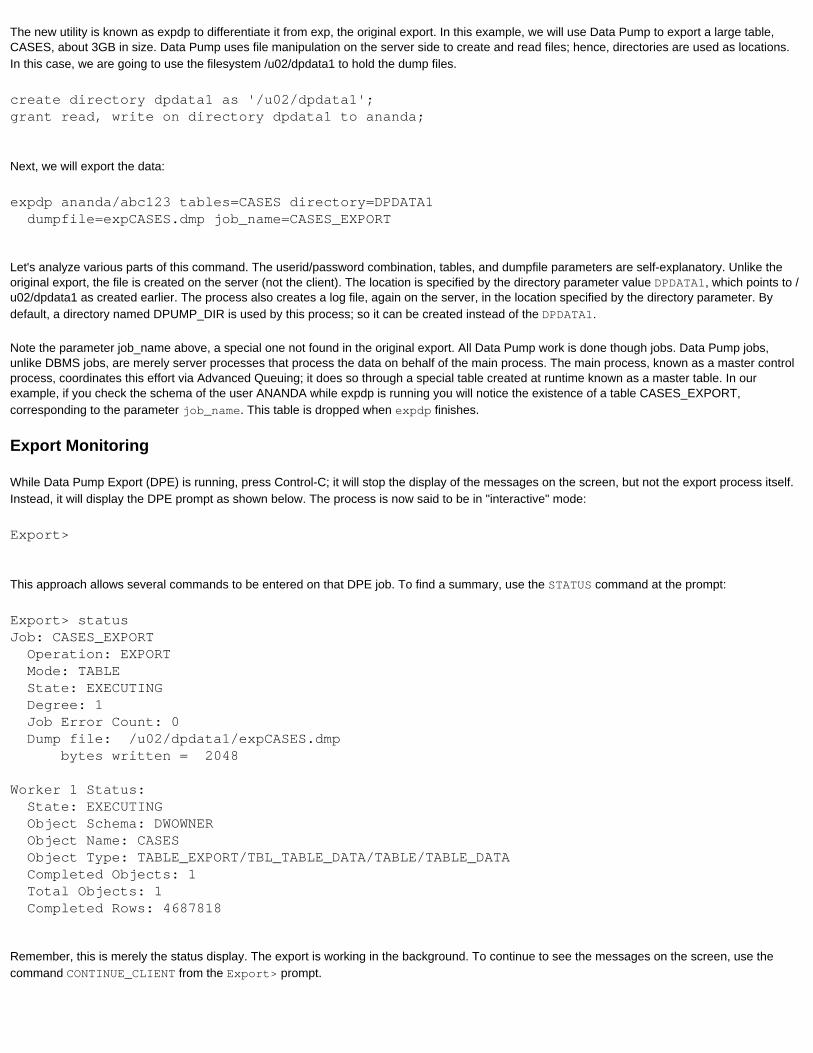
The new utility is known as expdp to differentiate it from exp, the original export. In this example, we will use Data Pump to export a large table, CASES, about 3GB in size. Data Pump uses file manipulation on the server side to create and read files; hence, directories are used as locations. In this case, we are going to use the filesystem /u02/dpdata1 to hold the dump files.

create directory dpdata1 as '/u02/dpdata1';grant read, write on directory dpdata1 to ananda;

Next, we will export the data:

expdp ananda/abc123 tables=CASES directory=DPDATA1 dumpfile=expCASES.dmp job_name=CASES_EXPORT

Let's analyze various parts of this command. The userid/password combination, tables, and dumpfile parameters are self-explanatory. Unlike the original export, the file is created on the server (not the client). The location is specified by the directory parameter value DPDATA1, which points to /u02/dpdata1 as created earlier. The process also creates a log file, again on the server, in the location specified by the directory parameter. By default, a directory named DPUMP_DIR is used by this process; so it can be created instead of the DPDATA1.

Note the parameter job_name above, a special one not found in the original export. All Data Pump work is done though jobs. Data Pump jobs, unlike DBMS jobs, are merely server processes that process the data on behalf of the main process. The main process, known as a master control process, coordinates this effort via Advanced Queuing; it does so through a special table created at runtime known as a master table. In our example, if you check the schema of the user ANANDA while expdp is running you will notice the existence of a table CASES_EXPORT, corresponding to the parameter job_name. This table is dropped when expdp finishes.

Export Monitoring

While Data Pump Export (DPE) is running, press Control-C; it will stop the display of the messages on the screen, but not the export process itself. Instead, it will display the DPE prompt as shown below. The process is now said to be in "interactive" mode:

Export>

This approach allows several commands to be entered on that DPE job. To find a summary, use the STATUS command at the prompt:

Export> statusJob: CASES_EXPORT Operation: EXPORT Mode: TABLE State: EXECUTING Degree: 1 Job Error Count: 0 Dump file: /u02/dpdata1/expCASES.dmp bytes written = 2048

Worker 1 Status: State: EXECUTING Object Schema: DWOWNER Object Name: CASES Object Type: TABLE_EXPORT/TBL_TABLE_DATA/TABLE/TABLE_DATA Completed Objects: 1 Total Objects: 1 Completed Rows: 4687818

Remember, this is merely the status display. The export is working in the background. To continue to see the messages on the screen, use the command CONTINUE_CLIENT from the Export> prompt.

Parallel Operation

You can accelerate jobs significantly using more than one thread for the export, through the PARALLEL parameter. Each thread creates a separate dumpfile, so the parameter dumpfile should have as many entries as the degree of parallelism. Instead of entering each one explicitly, you can specify wildcard characters as filenames such as:

expdp ananda/abc123 tables=CASES directory=DPDATA1 dumpfile=expCASES_%U.dmp parallel=4 job_name=Cases_Export

Note how the dumpfile parameter has a wild card %U, which indicates the files will be created as needed and the format will be expCASES_nn.dmp, where nn starts at 01 and goes up as needed.

In parallel mode, the status screen will show four worker processes. (In default mode, only one process will be visible.) All worker processes extract data simultaneously and show their progress on the status screen.

It's important to separate the I/O channels for access to the database files and the dumpfile directory filesystems. Otherwise, the overhead associated with maintaining the Data Pump jobs may outweigh the benefits of parallel threads and hence degrade performance. Parallelism will be in effect only if the number of tables is higher than the parallel value and the tables are big.

Database Monitoring

You can get more information on the Data Pump jobs running from the database views, too. The main view to monitor the jobs is DBA_DATAPUMP_JOBS, which tells you how many worker processes (column DEGREE) are working on the job. The other view that is important is DBA_DATAPUMP_SESSIONS, which when joined with the previous view and V$SESSION gives the SID of the session of the main foreground process.

select sid, serial#from v$session s, dba_datapump_sessions dwhere s.saddr = d.saddr;

This instruction shows the session of the foreground process. More useful information is obtained from the alert log. When the process starts up, the MCP and the worker processes are shown in the alert log as follows:

kupprdp: master process DM00 started with pid=23, OS id=20530 to execute - SYS.KUPM$MCP.MAIN('CASES_EXPORT', 'ANANDA');

kupprdp: worker process DW01 started with worker id=1, pid=24, OS id=20532 to execute - SYS.KUPW$WORKER.MAIN('CASES_EXPORT', 'ANANDA');

kupprdp: worker process DW03 started with worker id=2, pid=25, OS id=20534 to execute - SYS.KUPW$WORKER.MAIN('CASES_EXPORT', 'ANANDA');

It shows the PID of the sessions started for the data pump operation. You can find the actual SIDs using this query:

select sid, program from v$session where paddr in (select addr from v$process where pid in (23,24,25));

The PROGRAM column will show the process DM (for master process) or DW (the worker proceses), corresponding to the names in the alert log file. If a parallel query is used by a worker process, say for SID 23, you can see it in the view V$PX_SESSION to find it out. It will show you all the parallel query sessions running from the worker process represented by SID 23:

select sid from v$px_session where qcsid = 23;

Additional useful information can be obtained from the view V$SESSION_LONGOPS to predict the time it will take to complete the job.

select sid, serial#, sofar, totalworkfrom v$session_longopswhere opname = 'CASES_EXPORT'and sofar != totalwork;

The column totalwork shows the total amount of work, of which the sofar amount has been done up until now--which you can then use to estimate how much longer it will take.

Data Pump Import

Data import performance is where Data Pump really stands out, however. To import the data exported earlier, we will use

impdp ananda/abc123 directory=dpdata1 dumpfile=expCASES.dmp job_name=cases_import

The default behavior of the import process is to create the table and all associated objects, and to produce an error when the table exists. Should you want to append the data to the existing table, you could use TABLE_EXISTS_ACTION=APPEND in the above command line.

As with Data Pump Export, pressing Control-C on the process brings up the interactive mode of Date Pump Import (DPI); again, the prompt is Import>.

Operating on Specific Objects

Ever had a need to export only certain procedures from one user to be recreated in a different database or user? Unlike the traditional export utility, Data Pump allows you to export only a particular type of object. For instance, the following command lets you export only procedures, and nothing else--no tables, views, or even functions:

expdp ananda/iclaim directory=DPDATA1 dumpfile=expprocs.dmp include=PROCEDURE

To export only a few specific objects--say, function FUNC1 and procedure PROC1--you could use

expdp ananda/iclaim directory=DPDATA1 dumpfile=expprocs.dmp include=PROCEDURE:\"=\'PROC1\'\",FUNCTION:\"=\'FUNC1\'\"

This dumpfile serves as a backup of the sources. You can even use it to create DDL scripts to be used later. A special parameter called SQLFILE allows the creation of the DDL script file.

impdp ananda/iclaim directory=DPDATA1 dumpfile=expprocs.dmp sqlfile=procs.sql

This instruction creates a file named procs.sql in the directory specified by DPDATA1, containing the scripts of the objects inside the export dumpfile. This approach helps you create the sources quickly in another schema.

Using the parameter INCLUDE allows you to define objects to be included or excluded from the dumpfile. You can use the clause INCLUDE=TABLE:"LIKE 'TAB%'" to export only those tables whose name start with TAB. Similarly, you could use the construct INCLUDE=TABLE:"NOT LIKE 'TAB%'" to exclude all tables starting with TAB. Alternatively you can use the EXCLUDE parameter to exclude specific objects.

Data Pump can also be used to transport tablespaces using external tables; it's sufficiently powerful to redefine parallelism on the fly, attach more tables to an existing process, and so on (which are beyond the scope of this article; see Oracle Database Utilities 10g Release 1 10.1 for more details). The following command generates the list of all available parameters in the Data Pump export utility:

expdp help=y

Similarly, impdp help=y will show all the parameters in DPI.

While Data Pump jobs are running, you can pause them by issuing STOP_JOB on the DPE or DPI prompts and then restart them with START_JOB. This functionality comes in handy when you run out of space and want to make corrections before continuing.

For more information, read Part 1 of the Oracle Database Utilities 10g Release 1 10.1 guide.

Week 5Flashback Table

Reinstating an accidentally dropped table is effortless using the Flashback Table feature in Oracle Database 10g

Here's a scenario that happens more often than it should: a user drops a very important table--accidentally, of course--and it needs to be revived as soon as possible. (In some cases, this unfortunate user may even have been you, the DBA!)

Oracle9i Database introduced the concept of a Flashback Query option to retrieve data from a point in time in the past, but it can't flash back DDL operations such as dropping a table. The only recourse is to use tablespace point-in-time recovery in a different database and then recreate the table in the current database using export/import or some other method. This procedure demands significant DBA effort as well as precious time, not to mention the use of a different database for cloning.

Enter the Flashback Table feature in Oracle Database 10g, which makes the revival of a dropped table as easy as the execution of a few statements. Let's see how this feature works.

Drop That Table!

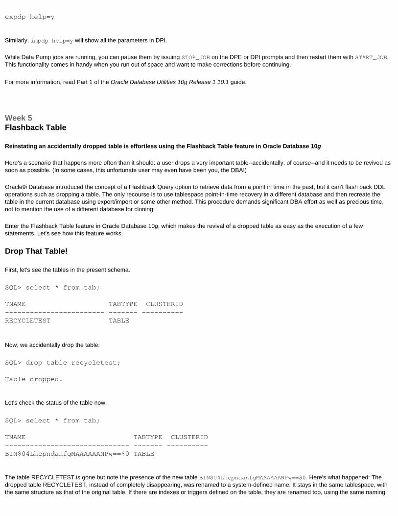
First, let's see the tables in the present schema.

SQL> select * from tab;

TNAME TABTYPE CLUSTERID------------------------ ------- ----------RECYCLETEST TABLE

Now, we accidentally drop the table:

SQL> drop table recycletest;

Table dropped.

Let's check the status of the table now.

SQL> select * from tab;

TNAME TABTYPE CLUSTERID------------------------------ ------- ----------BIN$04LhcpndanfgMAAAAAANPw==$0 TABLE

The table RECYCLETEST is gone but note the presence of the new table BIN$04LhcpndanfgMAAAAAANPw==$0. Here's what happened: The dropped table RECYCLETEST, instead of completely disappearing, was renamed to a system-defined name. It stays in the same tablespace, with the same structure as that of the original table. If there are indexes or triggers defined on the table, they are renamed too, using the same naming

convention used by the table. Any dependent sources such as procedures are invalidated; the triggers and indexes of the original table are instead placed on the renamed table BIN$04LhcpndanfgMAAAAAANPw==$0, preserving the complete object structure of the dropped table.

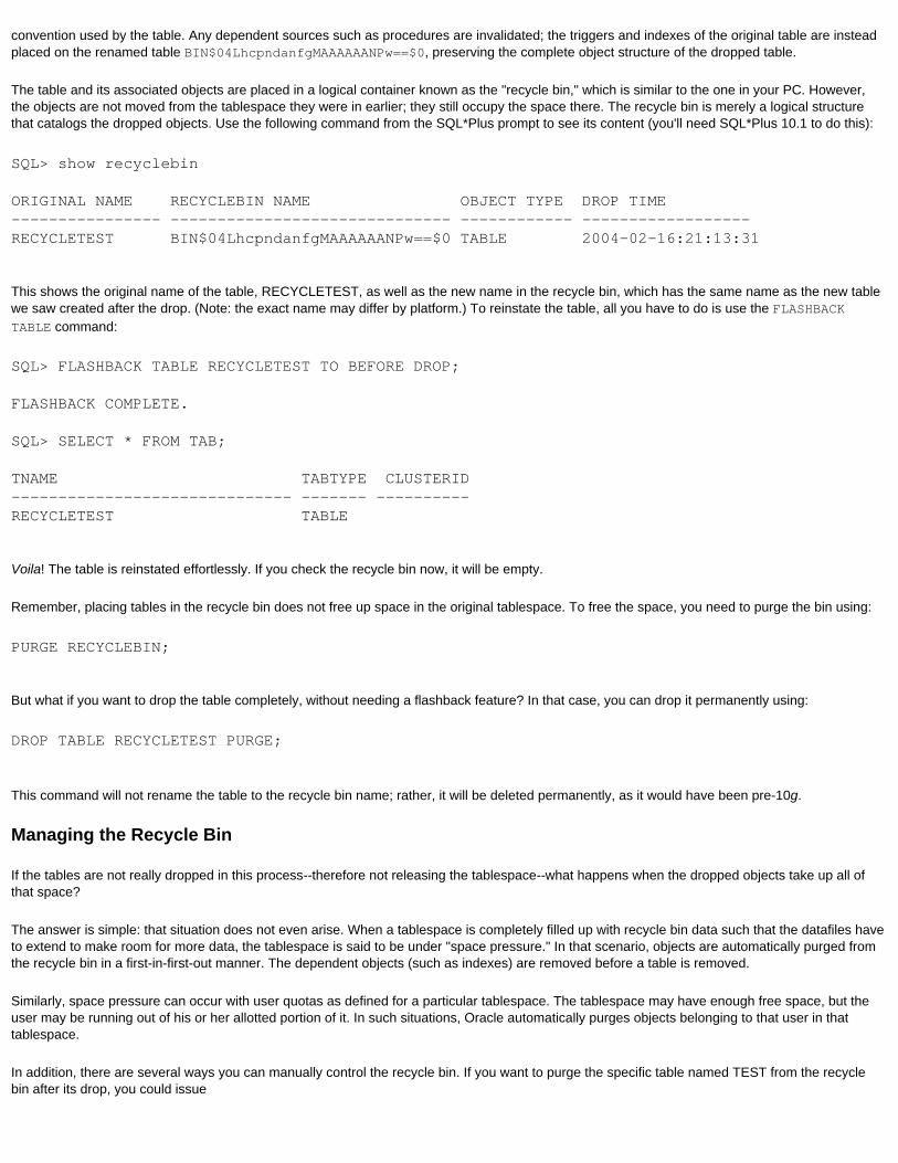
The table and its associated objects are placed in a logical container known as the "recycle bin," which is similar to the one in your PC. However, the objects are not moved from the tablespace they were in earlier; they still occupy the space there. The recycle bin is merely a logical structure that catalogs the dropped objects. Use the following command from the SQL*Plus prompt to see its content (you'll need SQL*Plus 10.1 to do this):

SQL> show recyclebin

ORIGINAL NAME RECYCLEBIN NAME OBJECT TYPE DROP TIME---------------- ------------------------------ ------------ ------------------RECYCLETEST BIN$04LhcpndanfgMAAAAAANPw==$0 TABLE 2004-02-16:21:13:31

This shows the original name of the table, RECYCLETEST, as well as the new name in the recycle bin, which has the same name as the new table we saw created after the drop. (Note: the exact name may differ by platform.) To reinstate the table, all you have to do is use the FLASHBACK TABLE command:

SQL> FLASHBACK TABLE RECYCLETEST TO BEFORE DROP;

FLASHBACK COMPLETE.

SQL> SELECT * FROM TAB;

TNAME TABTYPE CLUSTERID------------------------------ ------- ----------RECYCLETEST TABLE

Voila! The table is reinstated effortlessly. If you check the recycle bin now, it will be empty.

Remember, placing tables in the recycle bin does not free up space in the original tablespace. To free the space, you need to purge the bin using:

PURGE RECYCLEBIN;

But what if you want to drop the table completely, without needing a flashback feature? In that case, you can drop it permanently using:

DROP TABLE RECYCLETEST PURGE;

This command will not rename the table to the recycle bin name; rather, it will be deleted permanently, as it would have been pre-10g.

Managing the Recycle Bin

If the tables are not really dropped in this process--therefore not releasing the tablespace--what happens when the dropped objects take up all of that space?

The answer is simple: that situation does not even arise. When a tablespace is completely filled up with recycle bin data such that the datafiles have to extend to make room for more data, the tablespace is said to be under "space pressure." In that scenario, objects are automatically purged from the recycle bin in a first-in-first-out manner. The dependent objects (such as indexes) are removed before a table is removed.

Similarly, space pressure can occur with user quotas as defined for a particular tablespace. The tablespace may have enough free space, but the user may be running out of his or her allotted portion of it. In such situations, Oracle automatically purges objects belonging to that user in that tablespace.

In addition, there are several ways you can manually control the recycle bin. If you want to purge the specific table named TEST from the recycle bin after its drop, you could issue

PURGE TABLE TEST;

or using its recycle bin name:

PURGE TABLE "BIN$04LhcpndanfgMAAAAAANPw==$0";

This command will remove table TEST and all dependent objects such as indexes, constraints, and so on from the recycle bin, saving some space. If, however, you want to permanently drop an index from the recycle bin, you can do so using:

purge index in_test1_01;

which will remove the index only, leaving the copy of the table in the recycle bin.

Sometimes it might be useful to purge at a higher level. For instance, you may want to purge all the objects in recycle bin in a tablespace USERS. You would issue:

PURGE TABLESPACE USERS;

You may want to purge only the recycle bin for a particular user in that tablespace. This approach could come handy in data warehouse-type environments where users create and drop many transient tables. You could modify the command above to limit the purge to a specific user only:

PURGE TABLESPACE USERS USER SCOTT;

A user such as SCOTT would clear his own recycle bin with

PURGE RECYCLEBIN;

You as a DBA can purge all the objects in any tablespace using

PURGE DBA_RECYCLEBIN;

As you can see, the recycle bin can be managed in a variety of different ways to meet your specific needs.

Table Versions and Flashback

Oftentimes the user might create and drop the same table several times, as in:

CREATE TABLE TEST (COL1 NUMBER);INSERT INTO TEST VALUES (1);COMMIT;DROP TABLE TEST;CREATE TABLE TEST (COL1 NUMBER);INSERT INTO TEST VALUES (2);COMMIT;DROP TABLE TEST;CREATE TABLE TEST (COL1 NUMBER);INSERT INTO TEST VALUES (3);COMMIT;DROP TABLE TEST;

At this point, if you were to flash-back the table TEST, what would the value of the column COL1 be? Conventional thinking might suggest that the first version of the table is retrieved from the recycle bin, where the value of column COL1 is 1. Actually, the third version of the table is retrieved, not the first. So the column COL1 will have the value 3, not 1.

At this time you can also retrieve the other versions of the dropped table. However, the existence of a table TEST will not let that happen. You have two choices:

● Use the rename option:

FLASHBACK TABLE TEST TO BEFORE DROP RENAME TO TEST2;FLASHBACK TABLE TEST TO BEFORE DROP RENAME TO TEST1;

which will reinstate the first version of the table to TEST1 and the second versions to TEST2. The values of the column COL1 in TEST1 and TEST2 will be 1 and 2 respectively. Or,

● Use the specific recycle-bin names of the table to restore. To do that, first identify the table's recycle bin names and then issue:

FLASHBACK TABLE "BIN$04LhcpnoanfgMAAAAAANPw==$0" TO BEFORE DROP RENAME TO TEST2;FLASHBACK TABLE "BIN$04LhcpnqanfgMAAAAAANPw==$0" TO BEFORE DROP RENAME TO TEST1;

That will restore the two versions of the dropped table.

Be Warned...

The un-drop feature brings the table back to its original name, but not the associated objects like indexes and triggers, which are left with the recycled names. Sources such as views and procedures defined on the table are not recompiled and remain in the invalid state. These old names must be retrieved manually and then applied to the flashed-back table.

The information is kept in the view named USER_RECYCLEBIN. Before flashing-back the table, use the following query to retrieve the old names.

SELECT OBJECT_NAME, ORIGINAL_NAME, TYPEFROM USER_RECYCLEBINWHERE BASE_OBJECT = (SELECT BASE_OBJECT FROM USER_RECYCLEBINWHERE ORIGINAL_NAME = 'RECYCLETEST')AND ORIGINAL_NAME != 'RECYCLETEST';

OBJECT_NAME ORIGINAL_N TYPE------------------------------ ---------- --------BIN$04LhcpnianfgMAAAAAANPw==$0 IN_RT_01 INDEXBIN$04LhcpnganfgMAAAAAANPw==$0 TR_RT TRIGGER

After the table is flashed-back, the indexes and triggers on the table RECYCLETEST will be named as shown in the OBJECT_NAME column. From the above query, you can use the original name to rename the objects as follows:

ALTER INDEX "BIN$04LhcpnianfgMAAAAAANPw==$0" RENAME TO IN_RT_01;ALTER TRIGGER "BIN$04LhcpnganfgMAAAAAANPw==$0" RENAME TO TR_RT;

One notable exception is the bitmap indexes. When they are dropped, they are not placed in the recycle bin--hence they are not retrievable. The constraint names are also not retrievable from the view. They have to be renamed from other sources.

Other Uses of Flashback Tables

Flashback Drop Table is not limited to reversing the drop of the table. Similar to flashback queries, you can also use it to reinstate the table to a different point in time, replacing the entire table with its "past" version. For example, the following statement reinstates the table to a System Change Number (SCN) 2202666520.

FLASHBACK TABLE RECYCLETEST TO SCN 2202666520;

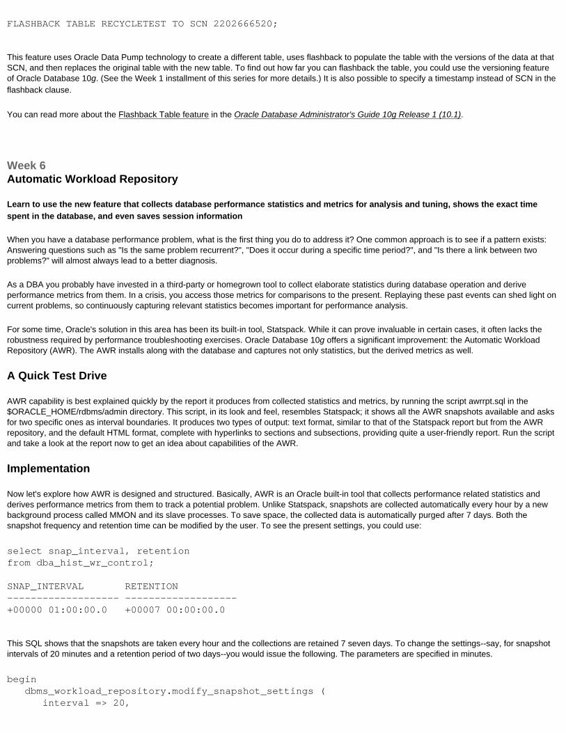
This feature uses Oracle Data Pump technology to create a different table, uses flashback to populate the table with the versions of the data at that SCN, and then replaces the original table with the new table. To find out how far you can flashback the table, you could use the versioning feature of Oracle Database 10g. (See the Week 1 installment of this series for more details.) It is also possible to specify a timestamp instead of SCN in the flashback clause.

You can read more about the Flashback Table feature in the Oracle Database Administrator's Guide 10g Release 1 (10.1).

Week 6Automatic Workload Repository

Learn to use the new feature that collects database performance statistics and metrics for analysis and tuning, shows the exact time spent in the database, and even saves session information

When you have a database performance problem, what is the first thing you do to address it? One common approach is to see if a pattern exists: Answering questions such as "Is the same problem recurrent?", "Does it occur during a specific time period?", and "Is there a link between two problems?" will almost always lead to a better diagnosis.

As a DBA you probably have invested in a third-party or homegrown tool to collect elaborate statistics during database operation and derive performance metrics from them. In a crisis, you access those metrics for comparisons to the present. Replaying these past events can shed light on current problems, so continuously capturing relevant statistics becomes important for performance analysis.

For some time, Oracle's solution in this area has been its built-in tool, Statspack. While it can prove invaluable in certain cases, it often lacks the robustness required by performance troubleshooting exercises. Oracle Database 10g offers a significant improvement: the Automatic Workload Repository (AWR). The AWR installs along with the database and captures not only statistics, but the derived metrics as well.

A Quick Test Drive

AWR capability is best explained quickly by the report it produces from collected statistics and metrics, by running the script awrrpt.sql in the $ORACLE_HOME/rdbms/admin directory. This script, in its look and feel, resembles Statspack; it shows all the AWR snapshots available and asks for two specific ones as interval boundaries. It produces two types of output: text format, similar to that of the Statspack report but from the AWR repository, and the default HTML format, complete with hyperlinks to sections and subsections, providing quite a user-friendly report. Run the script and take a look at the report now to get an idea about capabilities of the AWR.

Implementation

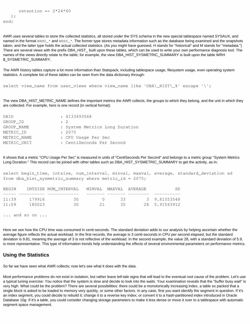
Now let's explore how AWR is designed and structured. Basically, AWR is an Oracle built-in tool that collects performance related statistics and derives performance metrics from them to track a potential problem. Unlike Statspack, snapshots are collected automatically every hour by a new background process called MMON and its slave processes. To save space, the collected data is automatically purged after 7 days. Both the snapshot frequency and retention time can be modified by the user. To see the present settings, you could use:

select snap_interval, retentionfrom dba_hist_wr_control;

SNAP_INTERVAL RETENTION------------------- -------------------+00000 01:00:00.0 +00007 00:00:00.0

This SQL shows that the snapshots are taken every hour and the collections are retained 7 seven days. To change the settings--say, for snapshot intervals of 20 minutes and a retention period of two days--you would issue the following. The parameters are specified in minutes.

begin dbms_workload_repository.modify_snapshot_settings ( interval => 20,

retention => 2*24*60 );end;

AWR uses several tables to store the collected statistics, all stored under the SYS schema in the new special tablespace named SYSAUX, and named in the format WRM$_* and WRH$_*. The former type stores metadata information such as the database being examined and the snapshots taken, and the latter type holds the actual collected statistics. (As you might have guessed, H stands for "historical" and M stands for "metadata.") There are several views with the prefix DBA_HIST_ built upon these tables, which can be used to write your own performance diagnosis tool. The names of the views directly relate to the table; for example, the view DBA_HIST_SYSMETRIC_SUMMARY is built upon the table WRH$_SYSMETRIC_SUMMARY.

The AWR history tables capture a lot more information than Statspack, including tablespace usage, filesystem usage, even operating system statistics. A complete list of these tables can be seen from the data dictionary through:

select view_name from user_views where view_name like 'DBA\_HIST\_%' escape '\';

The view DBA_HIST_METRIC_NAME defines the important metrics the AWR collects, the groups to which they belong, and the unit in which they are collected. For example, here is one record (in vertical format):

DBID : 4133493568GROUP_ID : 2GROUP_NAME : System Metrics Long DurationMETRIC_ID : 2075METRIC_NAME : CPU Usage Per SecMETRIC_UNIT : CentiSeconds Per Second

It shows that a metric "CPU Usage Per Sec" is measured in units of "CentiSeconds Per Second" and belongs to a metric group "System Metrics Long Duration." This record can be joined with other tables such as DBA_HIST_SYSMETRIC_SUMMARY to get the activity, as in:

select begin_time, intsize, num_interval, minval, maxval, average, standard_deviation sd from dba_hist_sysmetric_summary where metric_id = 2075;

BEGIN INTSIZE NUM_INTERVAL MINVAL MAXVAL AVERAGE SD----- ---------- ------------ ------- ------- -------- ----------11:39 179916 30 0 33 3 9.8155354811:09 180023 30 21 35 28 5.91543912

... and so on ...

Here we see how the CPU time was consumed in centi-seconds. The standard deviation adds to our analysis by helping ascertain whether the average figure reflects the actual workload. In the first records, the average is 3 centi-seconds in CPU per second elapsed, but the standard deviation is 9.81, meaning the average of 3 is not reflective of the workload. In the second example, the value 28, with a standard deviation of 5.9, is more representative. This type of information trends help understanding the effects of several environmental parameters on performance metrics.

Using the Statistics

So far we have seen what AWR collects; now let's see what it does with the data.

Most performance problems do not exist in isolation, but rather leave tell-tale signs that will lead to the eventual root cause of the problem. Let's use a typical tuning exercise: You notice that the system is slow and decide to look into the waits. Your examination reveals that the "buffer busy wait" is very high. What could be the problem? There are several possibilities: there could be a monotonically increasing index, a table so packed that a single block is asked to be loaded to memory very quickly, or some other factors. In any case, first you want identify the segment in question. If it's an index segment, you could decide to rebuild it; change it to a reverse key index; or convert it to a hash-partitioned index introduced in Oracle Database 10g. If it's a table, you could consider changing storage parameters to make it less dense or move it over to a tablespace with automatic segment space management.

Your plan of attack is generally methodical and usually based your knowledge of various events and your experience in dealing with them. Now imagine if the same thing were done by an engine - an engine that captures metrics and deduces possible plans based on pre-determined logic. Wouldn't your job be easier?

That engine, now available in Oracle Database 10g, is known as Automatic Database Diagnostic Monitor (ADDM). To arrive at a decision, ADDM uses the data collected by AWR. In the above discussion, ADDM can see that the buffer busy waits are occurring, pull the appropriate data to see the segments on which it occurs, evaluate its nature and composition, and finally offer solutions to the DBA. After each snapshot collection by AWR, the ADDM is invoked to examine the metrics and generate recommendations. So, in effect you have a full-time robotic DBA analyzing the data and generating recommendations proactively, freeing you to attend to more strategic issues.

To see the ADDM recommendations and the AWR repository data, use the new Enterprise Manager 10g console on the page named DB Home. To see the AWR reports, you can navigate to them from Administration, then Workload Repository, and then Snapshots. We'll examine ADDM in greater detail in a future installment.

You can also specify alerts to be generated based on certain conditions. These alerts, known as Server Generated Alerts, are pushed to an Advanced Queue, from where they can be consumed by any client listening to it. One such client is Enterprise Manager 10g, where the alerts are displayed prominently.

Time Model

When you have a performance problem, what comes to mind first to reduce the response time? Obviously, you want to eliminate (or reduce) the root cause of the factor that adds to the time. How do you know where the time was spent--not waiting, but actually doing the work?

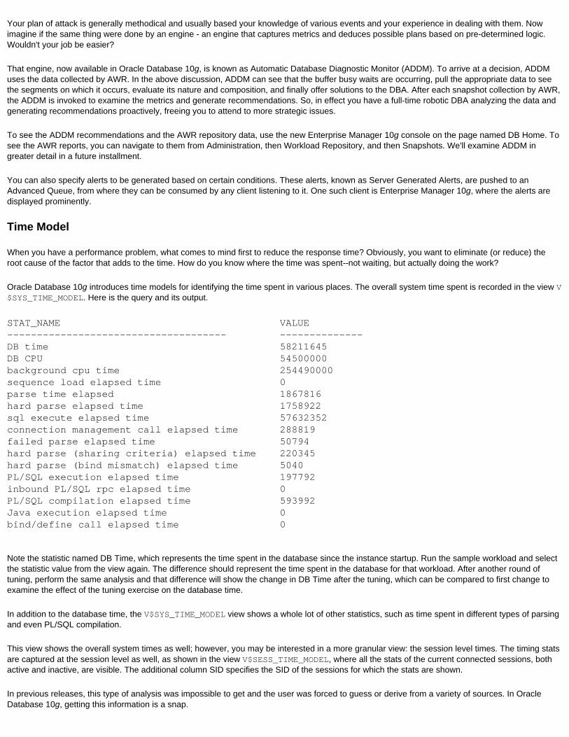
Oracle Database 10g introduces time models for identifying the time spent in various places. The overall system time spent is recorded in the view V$SYS_TIME_MODEL. Here is the query and its output.

STAT_NAME VALUE------------------------------------- --------------DB time 58211645DB CPU 54500000background cpu time 254490000sequence load elapsed time 0parse time elapsed 1867816hard parse elapsed time 1758922sql execute elapsed time 57632352connection management call elapsed time 288819failed parse elapsed time 50794hard parse (sharing criteria) elapsed time 220345hard parse (bind mismatch) elapsed time 5040PL/SQL execution elapsed time 197792inbound PL/SQL rpc elapsed time 0PL/SQL compilation elapsed time 593992Java execution elapsed time 0bind/define call elapsed time 0

Note the statistic named DB Time, which represents the time spent in the database since the instance startup. Run the sample workload and select the statistic value from the view again. The difference should represent the time spent in the database for that workload. After another round of tuning, perform the same analysis and that difference will show the change in DB Time after the tuning, which can be compared to first change to examine the effect of the tuning exercise on the database time.

In addition to the database time, the V$SYS_TIME_MODEL view shows a whole lot of other statistics, such as time spent in different types of parsing and even PL/SQL compilation.

This view shows the overall system times as well; however, you may be interested in a more granular view: the session level times. The timing stats are captured at the session level as well, as shown in the view V$SESS_TIME_MODEL, where all the stats of the current connected sessions, both active and inactive, are visible. The additional column SID specifies the SID of the sessions for which the stats are shown.

In previous releases, this type of analysis was impossible to get and the user was forced to guess or derive from a variety of sources. In Oracle Database 10g, getting this information is a snap.

Active Session History

The view V$SESSION in Oracle Database 10g has been improved; the most valuable improvement of them all is the inclusion of wait events and their duration, eliminating the need to see the view V$SESSION_WAIT. However, since this view merely reflects the values in real time, some of the important information is lost when it is viewed later. For instance, if you select from this view to check if any session is waiting for any non-idle event, and if so, the event in question, you may not find anything because the wait must have been over by the time you select it.

Enter the new feature Active Session History (ASH), which, like AWR, stores the session performance statistics in a buffer for analysis later. However, unlike AWR, the storage is not persistent in a table but in memory, and is shown in the view V$ACTIVE_SESSION_HISTORY. The data is polled every second and only the active sessions are polled. As time progresses, the old entries are removed to accommodate new ones in a circular buffer and shown in the view. To find out how many sessions waited for some event, you would use

select session_id||','||session_serial# SID, n.name, wait_time, time_waitedfrom v$active_session_history a, v$event_name nwhere n.event# = a.event#

This command tells you the name of the event and how much time was spent in waiting. If you want to drill down to a specific wait event, additional columns of ASH help you with that as well. For instance, if one of the events the sessions waited on is buffer busy wait, proper diagnosis must identify the segments on which the wait event occurred. You get that from the ASH view column CURRENT_OBJ#, which can then be joined with DBA_OBJECTS to get the segments in question.

ASH also records parallel query server sessions, useful to diagnose the parallel query wait events. If the record is for a parallel query slave process, the SID of the coordinator server session is identified by QC_SESSION_ID column. The column SQL_ID records the ID of the SQL statement that produced the wait event, which can be joined with the V$SQL view to get the offending SQL statement. To facilitate the identification of the clients in a shared user environment like a web application, the CLIENT_ID column is also shown, which can be set by DBMS_SESSION.SET_IDENTIFIER.

Since ASH information is so valuable, wouldn't it be nice if it were stored in a persistent manner similar to AWR? Fortunately, it is; the information is flushed to the disk by the MMON slave to the AWR table, visible through the view DBA_HIST_ACTIVE_SESS_HISTORY.

Manual Collection

Snapshots are collected automatically by default, but you can also collect them on demand. All AWR functionality has been implemented in the package DBMS_WORKLOAD_REPOSITORY. To take a snapshot, simply issue:

execute dbms_workload_repository.create_snapshot

It immediately takes a snapshot, recorded in the table WRM$_SNAPSHOT. The metrics collected are for the TYPICAL level. If you want to collect more detailed statistics, you can set the parameter FLUSH_LEVEL to ALL in the above procedure. The stats are deleted automatically but can also be deleted manually by calling the procedure drop_snapshot_range().

Baseline

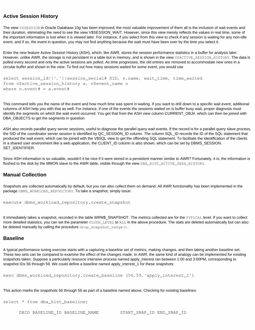
A typical performance tuning exercise starts with a capturing a baseline set of metrics, making changes, and then taking another baseline set. These two sets can be compared to examine the effect of the changes made. In AWR, the same kind of analogy can be implemented for existing snapshots taken. Suppose a particularly resource intensive process named apply_interest ran between 1:00 and 3:00PM, corresponding to snapshot IDs 56 through 59. We could define a baseline named apply_interest_1 for these snapshots:

exec dbms_workload_repository.create_baseline (56,59,'apply_interest_1')

This action marks the snapshots 56 through 59 as part of a baseline named above. Checking for existing baselines:

select * from dba_hist_baseline;

DBID BASELINE_ID BASELINE_NAME START_SNAP_ID END_SNAP_ID

---------- ----------- -------------------- ------------- -----------4133493568 1 apply_interest_1 56 59

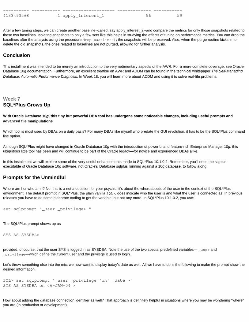
After a few tuning steps, we can create another baseline--called, say apply_interest_2--and compare the metrics for only those snapshots related to these two baselines. Isolating snapshots to only a few sets like this helps in studying the effects of tuning on performance metrics. You can drop the baselines after the analysis using the procedure drop_baseline(); the snapshots will be preserved. Also, when the purge routine kicks in to delete the old snapshots, the ones related to baselines are not purged, allowing for further analysis.

Conclusion

This installment was intended to be merely an introduction to the very rudimentary aspects of the AWR. For a more complete coverage, see Oracle Database 10g documentation. Furthermore, an excellent treatise on AWR and ADDM can be found in the technical whitepaper The Self-Managing Database: Automatic Performance Diagnosis. In Week 18, you will learn more about ADDM and using it to solve real-life problems.

Week 7SQL*Plus Grows Up

With Oracle Database 10g, this tiny but powerful DBA tool has undergone some noticeable changes, including useful prompts and advanced file manipulations

Which tool is most used by DBAs on a daily basis? For many DBAs like myself who predate the GUI revolution, it has to be the SQL*Plus command line option.

Although SQL*Plus might have changed in Oracle Database 10g with the introduction of powerful and feature-rich Enterprise Manager 10g, this ubiquitous little tool has been and will continue to be part of the Oracle legacy—for novice and experienced DBAs alike.

In this installment we will explore some of the very useful enhancements made to SQL*Plus 10.1.0.2. Remember, you'll need the sqlplus executable of Oracle Database 10g software, not Oracle9i Database sqlplus running against a 10g database, to follow along.

Prompts for the Unmindful

Where am I or who am I? No, this is a not a question for your psychic; it's about the whereabouts of the user in the context of the SQL*Plus environment. The default prompt in SQL*Plus, the plain vanilla SQL>, does indicate who the user is and what the user is connected as. In previous releases you have to do some elaborate coding to get the variable, but not any more. In SQL*Plus 10.1.0.2, you use:

set sqlprompt "_user _privilege> "

The SQL*Plus prompt shows up as

SYS AS SYSDBA>

provided, of course, that the user SYS is logged in as SYSDBA. Note the use of the two special predefined variables— _user and _privilege—which define the current user and the privilege it used to login.

Let's throw something else into the mix: we now want to display today's date as well. All we have to do is the following to make the prompt show the desired information.

SQL> set sqlprompt "_user _privilege 'on' _date >"SYS AS SYSDBA on 06-JAN-04 >

How about adding the database connection identifier as well? That approach is definitely helpful in situations where you may be wondering "where" you are (in production or development).

SQL> set sqlprompt "_user 'on' _date 'at' _connect_identifier >"ANANDA on 06-JAN-04 at SMILEY >

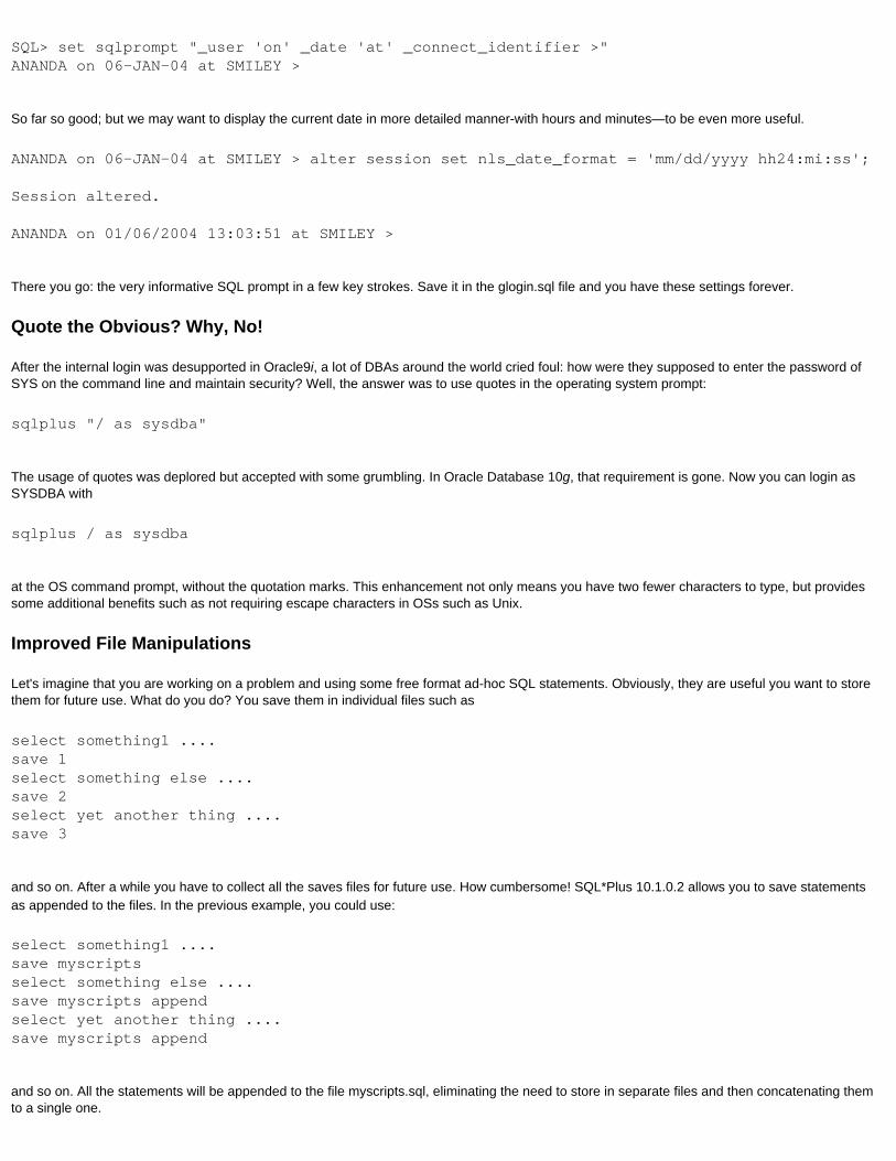
So far so good; but we may want to display the current date in more detailed manner-with hours and minutes—to be even more useful.

ANANDA on 06-JAN-04 at SMILEY > alter session set nls_date_format = 'mm/dd/yyyy hh24:mi:ss';

Session altered.

ANANDA on 01/06/2004 13:03:51 at SMILEY >

There you go: the very informative SQL prompt in a few key strokes. Save it in the glogin.sql file and you have these settings forever.

Quote the Obvious? Why, No!

After the internal login was desupported in Oracle9i, a lot of DBAs around the world cried foul: how were they supposed to enter the password of SYS on the command line and maintain security? Well, the answer was to use quotes in the operating system prompt:

sqlplus "/ as sysdba"

The usage of quotes was deplored but accepted with some grumbling. In Oracle Database 10g, that requirement is gone. Now you can login as SYSDBA with

sqlplus / as sysdba

at the OS command prompt, without the quotation marks. This enhancement not only means you have two fewer characters to type, but provides some additional benefits such as not requiring escape characters in OSs such as Unix.

Improved File Manipulations

Let's imagine that you are working on a problem and using some free format ad-hoc SQL statements. Obviously, they are useful you want to store them for future use. What do you do? You save them in individual files such as

select something1 ....save 1 select something else ....save 2select yet another thing ....save 3

and so on. After a while you have to collect all the saves files for future use. How cumbersome! SQL*Plus 10.1.0.2 allows you to save statements as appended to the files. In the previous example, you could use:

select something1 ....save myscriptsselect something else ....save myscripts appendselect yet another thing ....save myscripts append

and so on. All the statements will be appended to the file myscripts.sql, eliminating the need to store in separate files and then concatenating them to a single one.

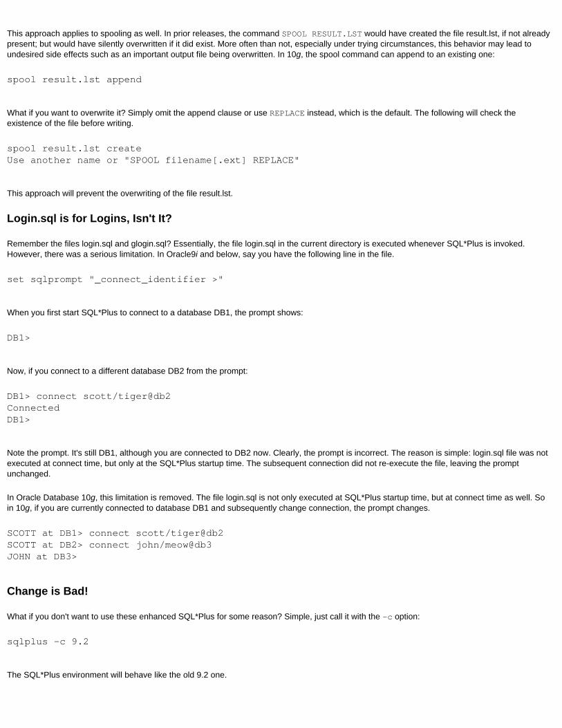
This approach applies to spooling as well. In prior releases, the command SPOOL RESULT.LST would have created the file result.lst, if not already present; but would have silently overwritten if it did exist. More often than not, especially under trying circumstances, this behavior may lead to undesired side effects such as an important output file being overwritten. In 10g, the spool command can append to an existing one:

spool result.lst append

What if you want to overwrite it? Simply omit the append clause or use REPLACE instead, which is the default. The following will check the existence of the file before writing.

spool result.lst createUse another name or "SPOOL filename[.ext] REPLACE"

This approach will prevent the overwriting of the file result.lst.

Login.sql is for Logins, Isn't It?

Remember the files login.sql and glogin.sql? Essentially, the file login.sql in the current directory is executed whenever SQL*Plus is invoked. However, there was a serious limitation. In Oracle9i and below, say you have the following line in the file.

set sqlprompt "_connect_identifier >"

When you first start SQL*Plus to connect to a database DB1, the prompt shows:

DB1>

Now, if you connect to a different database DB2 from the prompt:

DB1> connect scott/tiger@db2ConnectedDB1>

Note the prompt. It's still DB1, although you are connected to DB2 now. Clearly, the prompt is incorrect. The reason is simple: login.sql file was not executed at connect time, but only at the SQL*Plus startup time. The subsequent connection did not re-execute the file, leaving the prompt unchanged.

In Oracle Database 10g, this limitation is removed. The file login.sql is not only executed at SQL*Plus startup time, but at connect time as well. So in 10g, if you are currently connected to database DB1 and subsequently change connection, the prompt changes.

SCOTT at DB1> connect scott/tiger@db2SCOTT at DB2> connect john/meow@db3JOHN at DB3>

Change is Bad!

What if you don't want to use these enhanced SQL*Plus for some reason? Simple, just call it with the -c option:

sqlplus -c 9.2

The SQL*Plus environment will behave like the old 9.2 one.

Use DUAL Freely

How many developers (and DBAs, too) do you think use this command often?

select USER into <some variable> from DUAL

Far too many, probably. Each call to the DUAL creates logical I/Os, which the database can do without. In some cases the call to DUAL is inevitable as in the line <somevariable> := USER. Because Oracle code treats DUAL as a special table, some ideas for tuning tables may not apply or be relevant.

Oracle Database 10g makes all that worry simply disappear: Because DUAL is a special table, the consistent gets are considerably reduced and the optimization plan is different as seen from the event 10046 trace.

In Oracle9i

Rows Execution Plan------- --------------------------------------------------- 0 SELECT STATEMENT GOAL: CHOOSE 1 TABLE ACCESS (FULL) OF 'DUAL'

In 10g

Rows Execution Plan------- --------------------------------------------------- 0 SELECT STATEMENT MODE: ALL_ROWS 0 FAST DUAL

Notice the use of the new FAST DUAL optimization plan, as opposed to the FULL TABLE SCAN of DUAL in Oracle9i. This improvement reduces the consistent reads significantly, benefiting applications that use the DUAL table frequently.

Note: Technically these DUAL improvements are implemented in the SQL Optimizer, but of course for many users SQL*Plus is the primary tool for manipulating SQL.

Other Useful Tidbits

Other SQL*Plus enhancements have been described elsewhere in this series. For instance, I covered RECYCLEBIN concepts in the Week 5 installment about Flashback Table.

Contrary to some widespread rumors, the COPY command is still available, although it will be obsolete in a future release. (Hmm...didn't we hear that in Oracle9i?) If you have scripts written with this command, don't lose heart; it's not only available but supported as well. Actually, it has been enhanced a bit on the error message-reporting front. If the table has a LONG column, COPY is the only way you can create a copy of the table; the usual Create Table As Select will not be able to process tables with columns of long datatype.

Week 8Automatic Storage Management

Finally, DBAs can free themselves from the mundane yet common tasks of adding, shifting, and removing storage disks at no additional cost

You just received a brand-new server and storage subsystem for a new Oracle database. Aside from operating system configuration, what is your most important before you can create the database? Obviously, it's creating the storage system layout—or more specifically, choosing a level of protection and then building the necessary Redundant Array of Inexpensive Disks (RAID) sets.

Setting up storage takes a significant amount of time during most database installations. Zeroing on a specific disk configuration from among the multiple possibilities requires careful planning and analysis, and, most important, intimate knowledge of storage technology, volume managers, and filesystems. The design tasks at this stage can be loosely described as follows (note that this list is merely representative; tasks will vary by configuration):

1. Confirm that storage is recognized at the OS level and determine the level of redundancy protection that might already be provided (hardware RAID).

2. Assemble and build logical volume groups and determine if striping or mirroring is also necessary. 3. Build a file system on the logical volumes created by the logical volume manager. 4. Set the ownership and privileges so that the Oracle process can open, read, and write to the devices. 5. Create a database on that filesystem while taking care to create special files such as redo logs, temporary tablespaces, and undo

tablespaces in non-RAID locations, if possible.

In most shops, the majority of these steps are executed by someone with lots of knowledge about the storage system. That "someone" is usually not the DBA.

Notice, however, that all these tasks—striping, mirroring, logical filesystem building—are done to serve only one type of server, our Oracle Database. So, wouldn't it make sense for Oracle to offer some techniques of its own to simplify or enhance the process?

Oracle Database 10g does exactly that. A new and exciting feature, Automatic Storage Management (ASM), lets DBAs execute many of the above tasks completely within the Oracle framework. Using ASM you can transform a bunch of disks to a highly scalable (and the stress is on the word scalable) and performant filesystem/volume manager using nothing more than what comes with Oracle Database 10g software at no extra cost. And, no, you don't need to be an expert in disk, volume managers, or file system management.

In this installment, you will learn enough about ASM basics to start using it in real-world applications. As you might guess, this powerful feature warrants a comprehensive discussion that would go far beyond our current word count, so if you want to learn more, I've listed some excellent sources of information at the conclusion.

What is ASM?

Let's say that you have 10 disks to be used in the database. With ASM, you don't have to create anything on the OS side; the feature will group a set of physical disks to a logical entity known as a diskgroup. A diskgroup is analogous to a striped (and optionally mirrored) filesystem, with important differences: it's not a general-purpose filesystem for storing user files and it's not buffered. Because of the latter, a diskgroup offers the advantage of direct access to this space as a raw device yet provides the convenience and flexibility of a filesystem.

Logical volume managers typically use a function, such as hashing to map the logical address of the blocks to the physical blocks. This computation uses CPU cycles. Furthermore, when a new disk (or RAID-5 set of disks) is added, this typical striping function requires each bit of the entire data set to be relocated.

In contrast, ASM uses a special Oracle Instance to address the mapping of the file extents to the physical disk blocks. This design, in addition to being fast in locating the file extents, helps while adding or removing disks because the locations of file extents need not be coordinated. This special ASM instance is similar to other filesystems in that it must be running for ASM to work and can't be modified by the user. One ASM instance can service a number of Oracle databases instances on the same server.

This special instance is just that: an instance, not a database where users can create objects. All the metadata about the disks are stored in the diskgroups themselves, making them as self-describing as possible.

So in a nutshell, what are the advantages of ASM?

● Disk Addition—Adding a disk becomes very easy. No downtime is required and file extents are redistributed automatically. ● I/O Distribution—I/O is spread over all the available disks automatically, without manual intervention, reducing chances of a hot spot.● Stripe Width—Striping can be fine grained as in Redo Log Files (128K for faster transfer rate) and coarse for datafiles (1MB for transfer of a

large number of blocks at one time).● Buffering—The ASM filesystem is not buffered, making it direct I/O capable by design.● Kernelized Asynch I/O—There is no special setup necessary to enable kernelized asynchronous I/O, without using raw or third-party

filesystems such as Veritas Quick I/O.● Mirroring—Software mirroring can be set up easily, if hardware mirroring is not available.

Creating an ASM-enabled Database, Step by Step

Here's a concrete example of how you would create an ASM-enabled database:

1. Set up an ASM Instance

You create an ASM instance via the Database Creation Assistant by specifying the following initialization parameter:

INSTANCE_TYPE = ASM

You should start the instance up when the server is booted, and it should be one of the last things stopped when the server is shut down.

By default the value of this parameter is RDBMS, for regular databases.

2. Set up a Disk Group

After starting the ASM instance, create a disk group with the available disks.

CREATE DISKGROUP dskgrp1EXTERNAL REDUNDANCYDISK'/dev/d1','/dev/d2','/dev/d3','/dev/d4',... and so on for all the specific disks ...;

In the above command, we have instructed the database to create a diskgroup named dksgrp1 with the physical disks named /dev/d1, /dev/d2, and so on. Instead of giving disks separately, you can also specify disk names in wildcards in the DISK clause as follows.

DISK '/dev/d*'

In the above command, we have specified a clause EXTERNAL REDUNDANCY, which indicates that the failure of a disk will bring down the diskgroup. This is usually the case when the redundancy is provided by the hardware, such as mirroring. If there is no hardware based redundancy, the ASM can be set up to create a special set of disks called failgroup in the diskgroup to provide that redundancy.

CREATE DISKGROUP dskgrp1NORMAL REDUNDANCYFAILGROUP failgrp1 DISK'/dev/d1','/dev/d2',FAILGROUP failgrp2 DISK'/dev/d3','/dev/d4';

Although it may appear as such, d3 and d4 are not mirrors of d1 and d2. Rather, ASM uses all the disks to create a fault-tolerant system. For instance, a file on the diskgroup might be created in d1 with a copy maintained on d4. A second file may be created on d3 with copy on d2, and so on. Failure of a specific disk allows a copy on another disk so that the operation can continue. For example, you could lose the controller for both disks d1 and d2 and ASM would mirror copies of the extents across the failure group to maintain data integrity.

3. Create Tablespace

Now create a tablespace in the main database using a datafile in the ASM-enabled storage.

CREATE TABLESPACE USER_DATA DATAFILE '+dskgrp1/user_data_01'

SIZE 1024M/

That's it! The setup process is complete.

Note how the diskgroup is used as a virtual filesystem. This approach is useful not only in data files, but in other types of Oracle files as well. For instance, you could create online redo log files as

LOGFILE GROUP 1 ( '+dskgrp1/redo/group_1.258.3', '+dskgrp2/redo/group_1.258.3' ) SIZE 50M,...

Further Resources

As mentioned earlier, this article is not designed to offer all that is to know about the ASM feature and make you an expert, simply due to the sheer volume of information associated. However, don't despair; there is plenty of help available here on Oracle Technology Network:

"Storage on Automatic," by Lannes Morris-Murphy, is an excellent introductory article on ASM.

ASMLib, a library of the ASM features for Linux, extends ASM functionality. This page also links to technical references and source code for the library modules.

Chapter 12 of the Oracle Database Administrator's Guide 10g Release 1 (10.1) fully explains the concepts behind ASM.

Even archived log destinations can also be set to a diskgroup. Pretty much everything related to Oracle Database can be created in an ASM-based diskgroup. For example, backup is another great use of ASM. You can set up a bunch of inexpensive disks to create the recovery area of a database, which can be used by RMAN to create backup datafiles and archived log files. (In the next installment about RMAN in Oracle Database 10g, you'll learn in detail how to use that capability to your advantage.)

Please bear in mind however that ASM supports files created by and read by the Oracle Database only; it is not a replacement for a general-purpose filesystem and cannot store binaries or flat files.

Maintenance

Let's examine some typical tasks needed to maintain the diskgroups. From time to time, you may have to add additional disks into the diskgroup dskgrp1 to accommodate growing demand. You would issue:

alter diskgroup dskgrp1 add disk '/dev/d5';

To find out what disks are in what diskgroup, you would issue:

select * from v$asm_disk;

This command shows all the disks managed by the ASM instance for all the client databases. Of these disks, you may decide to remove a disk with:

alter diskgroup dskgrp1 drop disk diskb23;

Conclusion

The introduction of ASM provides a significant value in making it much easier to manage files in an Oracle database. Using this bundled feature, you can easily create a very scalable and performant storage solution from a set of disks. Any dynamic database environment requires the addition, shifting, and removal of disks, and ASM provides the necessary toolset to free the DBA from those mundane tasks.

Week 9RMAN

RMAN becomes more powerful with a redesigned incremental backup scheme, offline recovery of incremental backups, previewing

restore, recovering through resetlogs, file compression, and much more

Most people would agree that RMAN is the de facto tool of choice for Oracle database backup. But as powerful as they were, early versions of RMAN left something to be desired. Like many DBAs, I had pet peeves about the absence of what I consider to be must-have features.

Fortunately, Oracle Database 10g addresses many of these issues by incorporating many desirable features, making RMAN an even more powerful and useful tool. Let's take a look.

Incremental Backups Revisited

RMAN includes an option for incremental backups. But truthfully, how often do you use it? Probably occasionally, or possibly even never.

This option instructs the tool to back up blocks that have changed since the last incremental backup at the same level or below. For instance, a full backup (level_0) is taken on day 1 and two incrementals of level_1 are taken on days 2 and 3. The latter two merely back up the changed blocks between days 1 and 2 and days 2 and 3, not across the entire backup time. This strategy reduces backup size, requiring less space, and narrows the backup window, reducing the amount of data moving across the network.

The most important reason for doing incremental backups is associated with data warehouse environments, where many operations are done in NOLOGGING mode and data changes do not go to the archived log files—hence, no media recovery is possible. Considering the massive size of data warehouses today, and the fact that most of the data in them does not change, full backups are neither desirable nor practical. Rather, doing incremental backups in RMAN is an ideal alternative.

So why do many DBAs do incremental backups only rarely? One reason is that in Oracle9i and below, RMAN scans all the data blocks to identify candidates for backup. This process puts so much stress on the system that doing incrementals becomes impractical.

Oracle Database 10g RMAN implements incremental backups in a manner that disposes of that objection. It uses a file, analogous to journals in filesystems, to track the blocks that have changed since the last backup. RMAN reads this file to determine which blocks are to be backed up.

You can enable this tracking mechanism by issuing the following command:

SQL> alter database enable block change tracking using file '/rman_bkups/change.log';

This command creates a binary file called /rman_bkups/change.log for tracking purposes. Conversely, you can disable tracking with

SQL> alter database disable block change tracking;

To see whether change tracking is currently enabled, you can query:

SQL> select filename, status from v$block_change_tracking;

Flash Recovery Area

Flashback queries, introduced in Oracle9i, depend on undo tablespace to flash-back to a prior version, thereby limiting its ability go too far into the past. Flash recovery provided an alternative solution by creating flashback logs, which are similar to redo logs, to revert the database to a prior state. In summary, you create a flash recovery area for the database, specify its size, and place the database in flash recovery mode with the following SQL commands:

alter system set db_recovery_file_dest = '/ora_flash_area';alter system set db_recovery_file_dest_size = 2g;alter system set db_flashback_retention_target = 1440;alter database flashback on;

The database must be in archive log mode to be flashback-enabled. That process creates Oracle Managed Files in the directory /ora_flash_area, with a total size of up to 2GB. The database changes are written to these files and can be used to quickly recover the database to a point in the past.

By default, RMAN also uses /ora_flash_area to store backup files; thus, RMAN backups are stored on disk, not tape. For that reason, you have the ability to specify how many days you need to keep backups. After that period, the files are automatically deleted if more space is required.

The flash recovery area needn't be a filesystem or a directory, however—alternatively, it could be an Automatic Storage Management (ASM) diskgroup. In that case, the flash recovery area is specified by:

alter system set db_recovery_file_dest = '+dskgrp1';

Consequently, using ASM and RMAN in combination, you can build a highly scaleable, fault-tolerant storage system using cheap disks such as Serial ATA or SCSI drives, with no additional software required. (For more details about ASM, see the Week 8 installment in this series.) This approach not only makes the backup process much faster but also cheap enough to compete with the tape-based approach.

An additional benefit is protection against user errors. Because ASM files are not true filesystems, they are less likely to be corrupted accidentally by DBAs and sysadmins.

Incremental Merge

Let's say you have the following backup schedule:

Sunday - Level 0 (full), with tag level_0Monday - Level 1 (incremental) with tag level_1_monTuesday - Level 1 (incremental) with tag level_1_tue

and so on. If the database fails on Saturday, prior to 10g you would have had to restore the tag level_0 and then apply all six incrementals. It would have taken a long time, which is another reason many DBAs shun incremental backups.

Oracle Database 10g RMAN radically changes that equation. Now, your incremental backup command looks like this:

RMAN> backup incremental level_1 for recover of copy with tag level_0 database;

Here we have instructed RMAN to make an incremental level_1 backup and merge that with the full backup copy with the tag level_0. After this command, level_0 becomes a full backup of that day.

So, on Tuesday, the backup with tag level_0, when merged with incremental level_1 backup, becomes identical to the full Tuesday backup. Similarly, the incremental taken on Saturday, when applied to the backup on disk, will be equivalent to a full level_0 Saturday backup. If the database fails on Saturday, you just need to restore the level_0 backup plus a few archive logs to bring the database into a consistent state; there is no need to apply additional incrementals. This approach cuts down recovery time dramatically, speeds backup, and eliminates the need to make a full database backup again.

Compressed Files

With disk-based backups in the flash recovery area, you still have a big limitation: disk space. Especially when going across a network—as is usually the case—it's advisable to create as small a backup set as possible. In Oracle Database 10g RMAN, you can compress files inside the backup command itself:

RMAN> backup as compressed backupset incremental level 1 database;

Note the use of the clause COMPRESSED. It compresses backup files with an important difference: while restoring, RMAN can read the files without uncompressing. To confirm compression, check for the following message in the output:

channel ORA_DISK_1: starting compressed incremental level 1 datafile backupset

Furthermore, you can verify that the backup was compressed by checking the RMAN list output:

RMAN> list output;

BS Key Type LV Size Device Type Elapsed Time Completion Time------- ---- -- ---------- ----------- ------------ ---------------3 Incr 1 2M DISK 00:00:00 26-FEB-04 BP Key: 3 Status: AVAILABLE Compressed: YES Tag: TAG20040226T100154 Piece Name: /ora_flash_area/SMILEY10/backupset/2004_02_26/o1_mf_ncsn1_TAG20040226T100154_03w2m3lr_.bkp Controlfile Included: Ckp SCN: 318556 Ckp time: 26-FEB-04 SPFILE Included: Modification time: 26-FEB-04

As with any compression process, this approach puts pressure on CPUs. As a tradeoff, you can keep more RMAN backups on disk that are readily available for restore-and-recover operations. Alternatively, you can make RMAN backups at the Physical Standby Database that can be used to recover the primary database. That approach will offload backup resourses to another host.

Look Before You Leap: Recovery Preview

In Oracle Database 10g, RMAN has gone one more step ahead by providing the ability to preview the backups required to perform a restore operation.

RMAN> restore database preview;

Listing 1 shows the output of this operation. You can also preview specific restore operations; for example:

restore tablespace users preview;

Preview allows you to ensure the recovery readiness of your backup infrastructure by making periodic and regular checks.

Resetlogs and Recovery

Let's imagine that you have lost the current online redo log files and you have to perform an incomplete database recovery—a rare but not unheard of situation. The biggest problem is resetlogs; after incomplete recovery you must open the database with the resetlogs clause, which sets the sequence number of the log threads to 1, making your earlier backups obsolete in RMAN and making the recovery operation more of a challenge.

In Oracle9i and below, if you need to restore the database to a version prior to resetlogs, you have to restore to a different incarnation. In Oracle Database 10g, you don't have to do that. Thanks to additional infrastructure in the control file, RMAN can now readily use all backups, before and after a resetlogs operation, to recover the Oracle database. There is no need to shut down the database to make a backup. This new capability means that the database can be re-opened immediately for the user community after a resetlogs operation.

Ready for RMAN

The enhancements in Oracle Database 10g RMAN make it an even more compelling tool in your backup strategy. The improvements to the incremental backup process alone make RMAN tough to ignore.

For more information about RMAN in 10g, see Chapter 4 of Oracle Database Backup and Recovery Basics 10g Release 1 (10.1).

Week 10Auditing Tells All

Oracle Database 10g auditing captures user activities at a very detailed level, which may obviate manual, trigger-based auditing

Suppose user Joe updates a row of the table as shown below, assuming he has update privileges on that table.

update SCOTT.EMP set salary = 12000 where empno = 123456;

How do you track this activity in the database? In Oracle9i Database and below, auditing captures only the "who" part of the activity, not the "what." For instance, it lets you know that Joe updated the table EMP owner by SCOTT, but it does not show that he updated the salary column for the table for employee number 123456. It does not show the value of the salary column before the change, either—to capture such detailed changes, you either have to write your own triggers to capture values before the change or fish them out of archived logs using Log Miner.

Both approaches allow you to track what was changed and record the values before the change but only at significant costs. Using triggers to write audit data can have a major performance impact; for that reason, in some cases (such as in third-party applications) user-defined triggers are forbidden. Log Miner does not affect performance but it does rely on the availability of archived logs to track changes.

Fine-grained auditing (FGA), introduced in Oracle9i, allowed recording of these row-level changes along with SCN numbers to reconstruct the old data, but they work for select statements only, not for DML such as update, insert, and delete. Therefore, prior to Oracle Database 10g, using triggers is the only reliable albeit unattractive choice for tracking user-initiated changes at the row level.

With the arrival of 10g, these limitations are gone, thanks to two significant changes to the auditing facility. Because two types of audits are involved—the standard audit (available in all versions) and the fine-grained audit (available in Oracle9i and up)—we'll address them separately and then see how they complement each other to provide a single, powerful tracking facility.

The New Stuff

First, FGA now supports DML statements in addition to selects. These changes are recorded in the same place, the table FGA_LOG$, and displayed through the view DBA_FGA_AUDIT_TRAIL. In addition to DMLs, you can now choose to trigger a trail only if all relevant columns are accessed, or even when a few of them are accessed. (For a detailed explanation of how FGA works in 10g, see my Technical Article on that subject.)

Standard auditing, implemented by the SQL command AUDIT, can be used to quickly and easily set up tracking for a specific object. For instance, if you wanted to track all the updates to the table EMP owned by Scott, you would issue:

audit UPDATE on SCOTT.EMP by access;

This command will record all updates on the table SCOTT.EMP by any user each time it occurs, in the audit trail table AUD$, visible through the view DBA_AUDIT_TRAIL.

This capability was available prior to 10g, too. However, in those releases, the information written to the trail was limited to a few pertinent items such as the user who issued the statement, the time, the terminal id, and so on; it lacked important information such as the value of the bind variables. In 10g, the auditing action captures many of these pieces of important information, in addition to what was collected in prior versions. The primary table for auditing, AUD$, contains several new columns to record them, and consequently the view DBA_AUDIT_TRAIL, as well. Let's take a look at each of them in detail.

EXTENDED_TIMESTAMP. This column records the timestamp of the audit record in the TIMESTAMP (6) format, which records time in Greenwich Mean Time (also known as Universal Coordinated Time) with seconds up to 9 places after the decimal point and with the Time Zone information. An example of the time stored in this format is shown below.

2004-3-13 18.10.13.123456000 -5:0

This indicates a date of March 13, 2004, at Eastern Standard Time in the U.S., which is 5 hours after the UTC (as denoted by -5.0).

The presence of time in this extended format helps pinpoint audit trails to a much narrower time span, enhancing their usefulness especially with databases that span multiple time zones.

GLOBAL_UID and PROXY_SESSIONID. When an identity management component such as Oracle Internet Directory is used for authentication, the users may be visible to the database in a slightly different manner. For example, they may be authenticated as enterprise users when presented to the database. Auditing these users will not record their enterprise userid in the USERNAME column of the view DBA_AUDIT_TRAIL, making that information useless. In Oracle Database 10g, the global (or enterprise) user uniqueid is recorded in the columns GLOBAL_UID without any further processing or setup. This column could be used to query the directory server to find complete details about the enterprise user.

Sometimes the enterprise users might connect to the database via a proxy user, especially in multi-tier applications. A user could be given proxy authentication through the command

alter user scott grant connect to appuser;

This command will allow the user SCOTT to connect as APPUSER to the database, as the proxy user. In that case, the column COMMENT_TEXT will record that fact by storing the value PROXY; but the session id of the proxy user will not be recorded anywhere, as of Oracle9i. In 10g, the column PROXY_SESSIONID records it for exact identification of the proxy session.

INSTANCE_NUMBER. In an Oracle Real Application Clusters (RAC) environment, it might be helpful to know to which specific instance the user was connected while making the changes. In 10g, this column records the instance number as specified by the initialization parameter file for that instance.

OS_PROCESS. In Oracle9i and below, only the SID values are recorded in the audit trail; not the operating system process id. However, the OS process id of server process may be necessary later in order to cross-reference a trace file, for example. In 10g, this value is also recorded in this column.

TRANSACTIONID. Here comes the most critical price of information. Suppose the user issues

update CLASS set size = 10 where class_id = 123;commit;

This command qualifies as a transaction entry and an audit record is generated. However, how do you know what the audit record really recorded? If the record was a transaction, the transaction id is stored in this column. You can use it to join the audit trail with the view FLASHBACK_TRANSACTION_QUERY. Here is a small sample of columns in this view.

select start_scn, start_timestamp, commit_scn, commit_timestamp, undo_change#, row_id, undo_sqlfrom flashback_transaction_querywhere xid = '<the transaction id>';

In addition to the usual statistics on that transaction, undo change#, rowid, and so on, 10g also records the SQL to undo the transaction changes, in the column UNDO_SQL and the rowid of the affected row shown in the column ROW_ID.

System Change Number. Finally, it comes to recording the values before the change. How do you do that? Taking a cue from FGA in Oracle9i, the values before the change can be obtained through flashback queries. But you need to know the System Change Number (SCN) for the change and it is captured in this column in audit trail. You could issue

select size from class as of SCN 123456where where class_id = 123;

This will show what the user saw or what the value was prior to the change.

Extended DB Auditing

Remember our original interest: to capture user-issued SQL statements and bind variables that are not captured in standard auditing. Enter the enhanced auditing in Oracle Database 10g, in which these tasks become as trivial as making a simple initialization parameter change. Just place the following line in parameter file.

audit_trail = db_extended

This parameter will enable recording of SQL text and the values of the bind variables, if used, in the columns. This value was not available in the earlier versions.

When Triggers Are Necessary

Avoiding False Positives. Audit trails are generated through autonomous transactions from the original transactions. Hence they are committed even if the original transactions are rolled back.

Here is a simple example to illustrate the point. Assume that we have set up auditing for UPDATEs on table CLASS. A user issues a statement to update a data value from 20 to 10 and then rolls it back as shown below.

update class set size = 10 where class_id = 123;rollback

Now the value of the column SIZE will be 20, not 10, as if the user never did anything. However, the audit trail will capture the change, even if it's rolled back. This may be undesirable in some cases, especially if there are lots of rollbacks by users. In such a case, you may have to use the trigger to capture only committed changes. If there were a trigger on the table CLASS to insert records into the user defined audit trail, upon rollback the audit trails would have been rolled back too.

Capturing Before-change Values. Oracle-provided audit trails do not show the values before and after the change. For instance, the above change will create an audit record that shows the statement and the SCN number at the change, but not the value before the change (20). The value can be obtained from the SCN number using flashback query, but it depends on the information being available in the undo segments. If the information is not captured within the limit specified by the undo_retention period, the prior values can never be retrieved. Using a trigger guarantees that the values are captured without dependence on the undo_retention period, and may prove useful at times. Under these two circumstances you may decide to continue using triggers to record the audit trails at a granular detail.

Uniform Audit Trail

Because FGA and standard auditing capture similar types of information, they provide a lot of significant information when used together. Oracle Database 10g combines the trails to a common trail known as DBA_COMMON_AUDIT_TRAIL, which is a UNION ALL view of the views DBA_AUDIT_TRAIL and DBA_FGA_AUDIT_TRAIL. However, there are some significant differences between the two types of audit.

Conclusion

In 10g, auditing has matured from a mere "action recorder" to a "fact-recording mechanism" that captures user activities at a very detailed level, which may obviate your need for manual trigger-based auditing. It also combines the trails of standard auditing and FGA, making it easier to track database access regardless of how it was generated.

For additional information, see Chapter 11 of the Oracle Database Security Guide 10g Release 1 (10.1).

Week 11Wait Interface

For immediate performance problems not yet captured by ADDM, the 10g wait interface provides valuable data for diagnosis

"The database is too slow!"

These words are usually uttered with grimness by an unhappy user. If you're like me, you've heard them way too many times in your DBA career.

Well, what do you do to address the problem? Apart from ignoring the user (a luxury that most of us cannot afford), your probable first line of attack is to see if any session is waiting for anything inside or outside the database.

Oracle provides a simple but elegant mechanism for doing that: the view V$SESSION_WAIT. This view reveals a variety of information to help your diagnosis, such as the events a session is waiting for or has waited for, and for how long and how many times. For instance, if the session is waiting for the event "db file sequential read," the columns P1 and P2 show the file_id and block_id for the block the session is waiting for.

For most wait events this view is sufficient, but it is hardly a robust tuning tool for at least two important reasons:

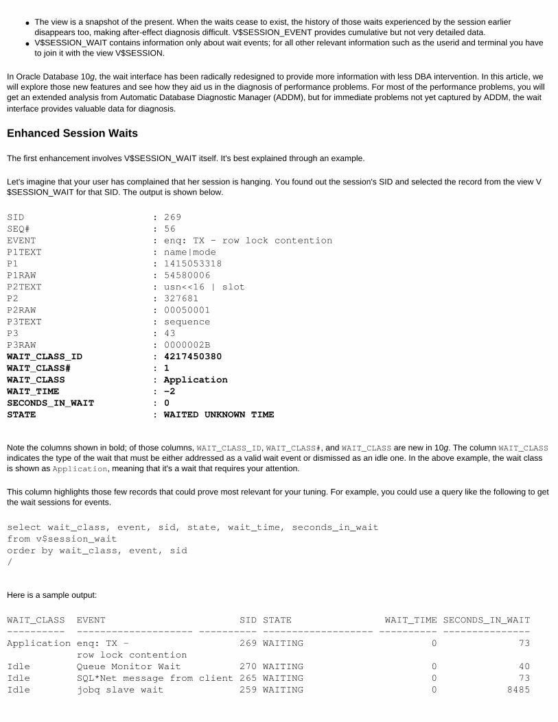
● The view is a snapshot of the present. When the waits cease to exist, the history of those waits experienced by the session earlier disappears too, making after-effect diagnosis difficult. V$SESSION_EVENT provides cumulative but not very detailed data.

● V$SESSION_WAIT contains information only about wait events; for all other relevant information such as the userid and terminal you have to join it with the view V$SESSION.

In Oracle Database 10g, the wait interface has been radically redesigned to provide more information with less DBA intervention. In this article, we will explore those new features and see how they aid us in the diagnosis of performance problems. For most of the performance problems, you will get an extended analysis from Automatic Database Diagnostic Manager (ADDM), but for immediate problems not yet captured by ADDM, the wait interface provides valuable data for diagnosis.

Enhanced Session Waits

The first enhancement involves V$SESSION_WAIT itself. It's best explained through an example.

Let's imagine that your user has complained that her session is hanging. You found out the session's SID and selected the record from the view V$SESSION_WAIT for that SID. The output is shown below.

SID : 269SEQ# : 56EVENT : enq: TX - row lock contentionP1TEXT : name|modeP1 : 1415053318P1RAW : 54580006P2TEXT : usn<<16 | slotP2 : 327681P2RAW : 00050001P3TEXT : sequenceP3 : 43P3RAW : 0000002BWAIT_CLASS_ID : 4217450380WAIT_CLASS# : 1WAIT_CLASS : ApplicationWAIT_TIME : -2SECONDS_IN_WAIT : 0STATE : WAITED UNKNOWN TIME

Note the columns shown in bold; of those columns, WAIT_CLASS_ID, WAIT_CLASS#, and WAIT_CLASS are new in 10g. The column WAIT_CLASS indicates the type of the wait that must be either addressed as a valid wait event or dismissed as an idle one. In the above example, the wait class is shown as Application, meaning that it's a wait that requires your attention.

This column highlights those few records that could prove most relevant for your tuning. For example, you could use a query like the following to get the wait sessions for events.

select wait_class, event, sid, state, wait_time, seconds_in_waitfrom v$session_waitorder by wait_class, event, sid/

Here is a sample output:

WAIT_CLASS EVENT SID STATE WAIT_TIME SECONDS_IN_WAIT---------- -------------------- ---------- ------------------- ---------- ---------------Application enq: TX - 269 WAITING 0 73 row lock contention Idle Queue Monitor Wait 270 WAITING 0 40Idle SQL*Net message from client 265 WAITING 0 73Idle jobq slave wait 259 WAITING 0 8485

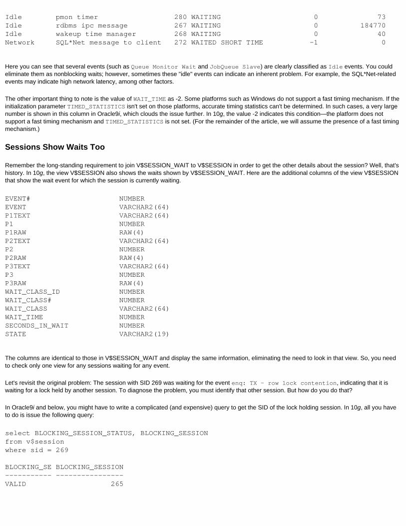
Idle pmon timer 280 WAITING 0 73Idle rdbms ipc message 267 WAITING 0 184770Idle wakeup time manager 268 WAITING 0 40Network SQL*Net message to client 272 WAITED SHORT TIME -1 0

Here you can see that several events (such as Queue Monitor Wait and JobQueue Slave) are clearly classified as Idle events. You could eliminate them as nonblocking waits; however, sometimes these "idle" events can indicate an inherent problem. For example, the SQL*Net-related events may indicate high network latency, among other factors.

The other important thing to note is the value of WAIT_TIME as -2. Some platforms such as Windows do not support a fast timing mechanism. If the initialization parameter TIMED_STATISTICS isn't set on those platforms, accurate timing statistics can't be determined. In such cases, a very large number is shown in this column in Oracle9i, which clouds the issue further. In 10g, the value -2 indicates this condition—the platform does not support a fast timing mechanism and TIMED_STATISTICS is not set. (For the remainder of the article, we will assume the presence of a fast timing mechanism.)

Sessions Show Waits Too

Remember the long-standing requirement to join V$SESSION_WAIT to V$SESSION in order to get the other details about the session? Well, that's history. In 10g, the view V$SESSION also shows the waits shown by V$SESSION_WAIT. Here are the additional columns of the view V$SESSION that show the wait event for which the session is currently waiting.

EVENT# NUMBEREVENT VARCHAR2(64)P1TEXT VARCHAR2(64)P1 NUMBERP1RAW RAW(4)P2TEXT VARCHAR2(64)P2 NUMBERP2RAW RAW(4)P3TEXT VARCHAR2(64)P3 NUMBERP3RAW RAW(4)WAIT_CLASS_ID NUMBERWAIT_CLASS# NUMBERWAIT_CLASS VARCHAR2(64)WAIT_TIME NUMBERSECONDS_IN_WAIT NUMBERSTATE VARCHAR2(19)

The columns are identical to those in V$SESSION_WAIT and display the same information, eliminating the need to look in that view. So, you need to check only one view for any sessions waiting for any event.

Let's revisit the original problem: The session with SID 269 was waiting for the event enq: TX - row lock contention, indicating that it is waiting for a lock held by another session. To diagnose the problem, you must identify that other session. But how do you do that?

In Oracle9i and below, you might have to write a complicated (and expensive) query to get the SID of the lock holding session. In 10g, all you have to do is issue the following query:

select BLOCKING_SESSION_STATUS, BLOCKING_SESSIONfrom v$session where sid = 269

BLOCKING_SE BLOCKING_SESSION----------- ----------------VALID 265

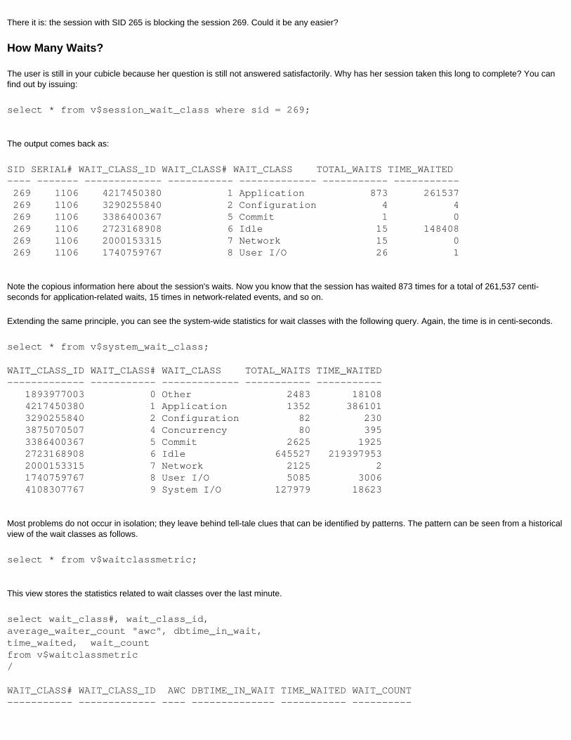
There it is: the session with SID 265 is blocking the session 269. Could it be any easier?

How Many Waits?

The user is still in your cubicle because her question is still not answered satisfactorily. Why has her session taken this long to complete? You can find out by issuing:

select * from v$session_wait_class where sid = 269;

The output comes back as:

SID SERIAL# WAIT_CLASS_ID WAIT_CLASS# WAIT_CLASS TOTAL_WAITS TIME_WAITED---- ------- ------------- ----------- ------------- ----------- ----------- 269 1106 4217450380 1 Application 873 261537 269 1106 3290255840 2 Configuration 4 4 269 1106 3386400367 5 Commit 1 0 269 1106 2723168908 6 Idle 15 148408 269 1106 2000153315 7 Network 15 0 269 1106 1740759767 8 User I/O 26 1

Note the copious information here about the session's waits. Now you know that the session has waited 873 times for a total of 261,537 centi-seconds for application-related waits, 15 times in network-related events, and so on.

Extending the same principle, you can see the system-wide statistics for wait classes with the following query. Again, the time is in centi-seconds.

select * from v$system_wait_class;

WAIT_CLASS_ID WAIT_CLASS# WAIT_CLASS TOTAL_WAITS TIME_WAITED------------- ----------- ------------- ----------- ----------- 1893977003 0 Other 2483 18108 4217450380 1 Application 1352 386101 3290255840 2 Configuration 82 230 3875070507 4 Concurrency 80 395 3386400367 5 Commit 2625 1925 2723168908 6 Idle 645527 219397953 2000153315 7 Network 2125 2 1740759767 8 User I/O 5085 3006 4108307767 9 System I/O 127979 18623

Most problems do not occur in isolation; they leave behind tell-tale clues that can be identified by patterns. The pattern can be seen from a historical view of the wait classes as follows.

select * from v$waitclassmetric;

This view stores the statistics related to wait classes over the last minute.

select wait_class#, wait_class_id, average_waiter_count "awc", dbtime_in_wait,time_waited, wait_countfrom v$waitclassmetric/

WAIT_CLASS# WAIT_CLASS_ID AWC DBTIME_IN_WAIT TIME_WAITED WAIT_COUNT----------- ------------- ---- -------------- ----------- ----------

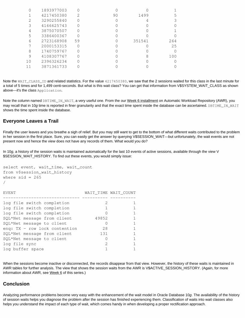
0 1893977003 0 0 0 1 1 4217450380 2 90 1499 5 2 3290255840 0 0 4 3 3 4166625743 0 0 0 0 4 3875070507 0 0 0 1 5 3386400367 0 0 0 0 6 2723168908 59 0 351541 264 7 2000153315 0 0 0 25 8 1740759767 0 0 0 0 9 4108307767 0 0 8 100 10 2396326234 0 0 0 0 11 3871361733 0 0 0 0

Note the WAIT_CLASS_ID and related statistics. For the value 4217450380, we saw that the 2 sessions waited for this class in the last minute for a total of 5 times and for 1,499 centi-seconds. But what is this wait class? You can get that information from V$SYSTEM_WAIT_CLASS as shown above—it's the class Application.

Note the column named DBTIME_IN_WAIT, a very useful one. From the our Week 6 installment on Automatic Workload Repository (AWR), you may recall that in 10g time is reported in finer granularity and that the exact time spent inside the database can be ascertained. DBTIME_IN_WAIT shows the time spent inside the database.

Everyone Leaves a Trail

Finally the user leaves and you breathe a sigh of relief. But you may still want to get to the bottom of what different waits contributed to the problem in her session in the first place. Sure, you can easily get the answer by querying V$SESSION_WAIT—but unfortunately, the wait events are not present now and hence the view does not have any records of them. What would you do?

In 10g, a history of the session waits is maintained automatically for the last 10 events of active sessions, available through the view V$SESSION_WAIT_HISTORY. To find out these events, you would simply issue:

select event, wait_time, wait_countfrom v$session_wait_historywhere sid = 265/

EVENT WAIT_TIME WAIT_COUNT------------------------------ ---------- ----------log file switch completion 2 1log file switch completion 1 1log file switch completion 0 1SQL*Net message from client 49852 1SQL*Net message to client 0 1enq: TX - row lock contention 28 1SQL*Net message from client 131 1SQL*Net message to client 0 1log file sync 2 1log buffer space 1 1

When the sessions become inactive or disconnected, the records disappear from that view. However, the history of these waits is maintained in AWR tables for further analysis. The view that shows the session waits from the AWR is V$ACTIVE_SESSION_HISTORY. (Again, for more information about AWR, see Week 6 of this series.)

Conclusion

Analyzing performance problems become very easy with the enhancement of the wait model in Oracle Database 10g. The availability of the history of session waits helps you diagnose the problem after the session has finished experiencing them. Classification of waits into wait classes also helps you understand the impact of each type of wait, which comes handy in when developing a proper rectification approach.

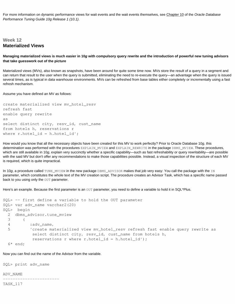
For more information on dynamic performance views for wait events and the wait events themselves, see Chapter 10 of the Oracle Database Performance Tuning Guide 10g Release 1 (10.1).

Week 12Materialized Views

Managing materialized views is much easier in 10g with compulsory query rewrite and the introduction of powerful new tuning advisors that take guesswork out of the picture

Materialized views (MVs), also known as snapshots, have been around for quite some time now. MVs store the result of a query in a segment and can return that result to the user when the query is submitted, eliminating the need to re-execute the query—an advantage when the query is issued several times, as is typical in data warehouse environments. MVs can be refreshed from base tables either completely or incrementally using a fast refresh mechanism.

Assume you have defined an MV as follows:

create materialized view mv_hotel_resvrefresh fastenable query rewriteasselect distinct city, resv_id, cust_namefrom hotels h, reservations r where r.hotel_id = h.hotel_id';

How would you know that all the necessary objects have been created for this MV to work perfectly? Prior to Oracle Database 10g, this determination was performed with the procedures EXPLAIN_MVIEW and EXPLAIN_REWRITE in the package DBMS_MVIEW. These procedures, which are still available in 10g, explain very succinctly whether a specific capability—such as fast refreshability or query rewritability—are possible with the said MV but don't offer any recommendations to make those capabilities possible. Instead, a visual inspection of the structure of each MV is required, which is quite impractical.

In 10g, a procedure called TUNE_MVIEW in the new package DBMS_ADVISOR makes that job very easy: You call the package with the IN parameter, which constitutes the whole text of the MV creation script. The procedure creates an Advisor Task, which has a specific name passed back to you using only the OUT parameter.

Here's an example. Because the first parameter is an OUT parameter, you need to define a variable to hold it in SQL*Plus.

SQL> -- first define a variable to hold the OUT parameterSQL> var adv_name varchar2(20)SQL> begin 2 dbms_advisor.tune_mview 3 ( 4 :adv_name, 5 'create materialized view mv_hotel_resv refresh fast enable query rewrite as select distinct city, resv_id, cust_name from hotels h, reservations r where r.hotel_id = h.hotel_id'); 6* end;

Now you can find out the name of the Advisor from the variable.

SQL> print adv_name

ADV_NAME-----------------------TASK_117

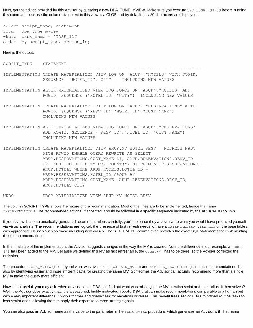
Next, get the advice provided by this Advisor by querying a new DBA_TUNE_MVIEW. Make sure you execute SET LONG 999999 before running this command because the column statement in this view is a CLOB and by default only 80 characters are displayed.

select script_type, statement from dba_tune_mview where task_name = 'TASK_117' order by script_type, action_id;

Here is the output:

SCRIPT_TYPE STATEMENT-------------- ------------------------------------------------------------IMPLEMENTATION CREATE MATERIALIZED VIEW LOG ON "ARUP"."HOTELS" WITH ROWID, SEQUENCE ("HOTEL_ID","CITY") INCLUDING NEW VALUES

IMPLEMENTATION ALTER MATERIALIZED VIEW LOG FORCE ON "ARUP"."HOTELS" ADD ROWID, SEQUENCE ("HOTEL_ID","CITY") INCLUDING NEW VALUES

IMPLEMENTATION CREATE MATERIALIZED VIEW LOG ON "ARUP"."RESERVATIONS" WITH ROWID, SEQUENCE ("RESV_ID","HOTEL_ID","CUST_NAME") INCLUDING NEW VALUES

IMPLEMENTATION ALTER MATERIALIZED VIEW LOG FORCE ON "ARUP"."RESERVATIONS" ADD ROWID, SEQUENCE ("RESV_ID","HOTEL_ID","CUST_NAME") INCLUDING NEW VALUES

IMPLEMENTATION CREATE MATERIALIZED VIEW ARUP.MV_HOTEL_RESV REFRESH FAST WITH ROWID ENABLE QUERY REWRITE AS SELECT ARUP.RESERVATIONS.CUST_NAME C1, ARUP.RESERVATIONS.RESV_ID C2, ARUP.HOTELS.CITY C3, COUNT(*) M1 FROM ARUP.RESERVATIONS, ARUP.HOTELS WHERE ARUP.HOTELS.HOTEL_ID = ARUP.RESERVATIONS.HOTEL_ID GROUP BY ARUP.RESERVATIONS.CUST_NAME, ARUP.RESERVATIONS.RESV_ID, ARUP.HOTELS.CITY

UNDO DROP MATERIALIZED VIEW ARUP.MV_HOTEL_RESV

The column SCRIPT_TYPE shows the nature of the recommendation. Most of the lines are to be implemented, hence the name IMPLEMENTATION. The recommended actions, if accepted, should be followed in a specific sequence indicated by the ACTION_ID column.

If you review these automatically-generated recommendations carefully, you'll note that they are similar to what you would have produced yourself via visual analysis. The recommendations are logical; the presence of fast refresh needs to have a MATERIALIZED VIEW LOG on the base tables with appropriate clauses such as those including new values. The STATEMENT column even provides the exact SQL statements for implementing these recommendations.

In the final step of the implementation, the Advisor suggests changes in the way the MV is created. Note the difference in our example: a count(*) has been added to the MV. Because we defined this MV as fast refreshable, the count(*) has to be there, so the Advisor corrected the omission.

The procedure TUNE_MVIEW goes beyond what was available in EXPLAIN_MVIEW and EXPLAIN_REWRITE not just in its recommendations, but also by identifying easier and more efficient paths for creating the same MV. Sometimes the Advisor can actually recommend more than a single MV to make the query more efficient.

How is that useful, you may ask, when any seasoned DBA can find out what was missing in the MV creation script and then adjust it themselves? Well, the Advisor does exactly that: it is a seasoned, highly motivated, robotic DBA that can make recommendations comparable to a human but with a very important difference: it works for free and doesn't ask for vacations or raises. This benefit frees senior DBAs to offload routine tasks to less senior ones, allowing them to apply their expertise to more strategic goals.

You can also pass an Advisor name as the value to the parameter in the TUNE_MVIEW procedure, which generates an Advisor with that name

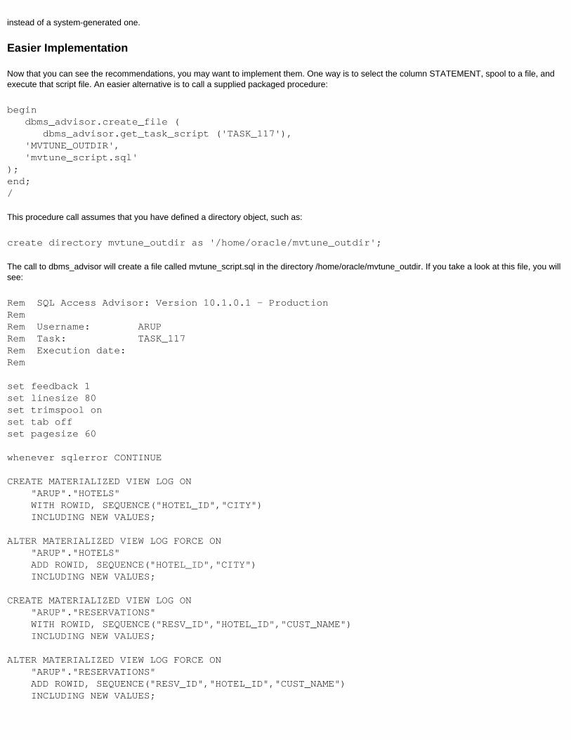
instead of a system-generated one.

Easier Implementation

Now that you can see the recommendations, you may want to implement them. One way is to select the column STATEMENT, spool to a file, and execute that script file. An easier alternative is to call a supplied packaged procedure:

begin dbms_advisor.create_file ( dbms_advisor.get_task_script ('TASK_117'), 'MVTUNE_OUTDIR', 'mvtune_script.sql');end;/

This procedure call assumes that you have defined a directory object, such as:

create directory mvtune_outdir as '/home/oracle/mvtune_outdir';

The call to dbms_advisor will create a file called mvtune_script.sql in the directory /home/oracle/mvtune_outdir. If you take a look at this file, you will see:

Rem SQL Access Advisor: Version 10.1.0.1 - ProductionRemRem Username: ARUPRem Task: TASK_117Rem Execution date:Rem

set feedback 1set linesize 80set trimspool onset tab offset pagesize 60

whenever sqlerror CONTINUE

CREATE MATERIALIZED VIEW LOG ON "ARUP"."HOTELS" WITH ROWID, SEQUENCE("HOTEL_ID","CITY") INCLUDING NEW VALUES;

ALTER MATERIALIZED VIEW LOG FORCE ON "ARUP"."HOTELS" ADD ROWID, SEQUENCE("HOTEL_ID","CITY") INCLUDING NEW VALUES;

CREATE MATERIALIZED VIEW LOG ON "ARUP"."RESERVATIONS" WITH ROWID, SEQUENCE("RESV_ID","HOTEL_ID","CUST_NAME") INCLUDING NEW VALUES;

ALTER MATERIALIZED VIEW LOG FORCE ON "ARUP"."RESERVATIONS" ADD ROWID, SEQUENCE("RESV_ID","HOTEL_ID","CUST_NAME") INCLUDING NEW VALUES;

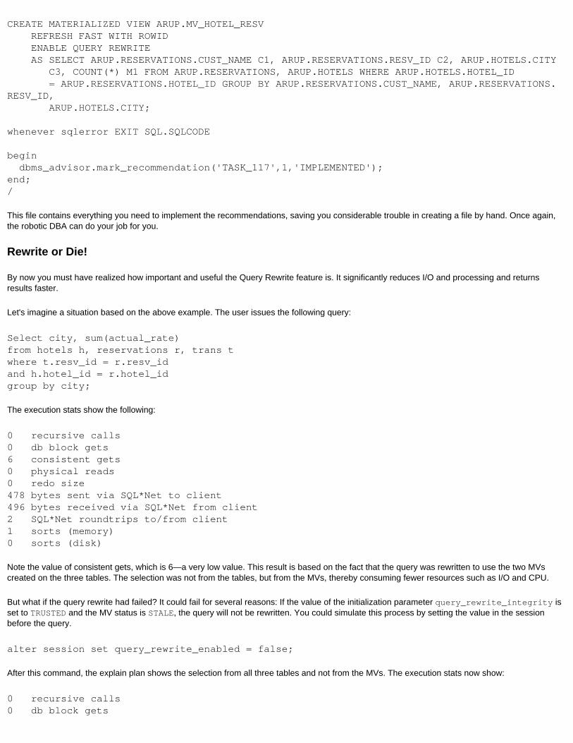
CREATE MATERIALIZED VIEW ARUP.MV_HOTEL_RESV REFRESH FAST WITH ROWID ENABLE QUERY REWRITE AS SELECT ARUP.RESERVATIONS.CUST_NAME C1, ARUP.RESERVATIONS.RESV_ID C2, ARUP.HOTELS.CITY C3, COUNT(*) M1 FROM ARUP.RESERVATIONS, ARUP.HOTELS WHERE ARUP.HOTELS.HOTEL_ID = ARUP.RESERVATIONS.HOTEL_ID GROUP BY ARUP.RESERVATIONS.CUST_NAME, ARUP.RESERVATIONS.RESV_ID, ARUP.HOTELS.CITY;

whenever sqlerror EXIT SQL.SQLCODE

begin dbms_advisor.mark_recommendation('TASK_117',1,'IMPLEMENTED');end;/

This file contains everything you need to implement the recommendations, saving you considerable trouble in creating a file by hand. Once again, the robotic DBA can do your job for you.

Rewrite or Die!

By now you must have realized how important and useful the Query Rewrite feature is. It significantly reduces I/O and processing and returns results faster.

Let's imagine a situation based on the above example. The user issues the following query:

Select city, sum(actual_rate)from hotels h, reservations r, trans twhere t.resv_id = r.resv_idand h.hotel_id = r.hotel_idgroup by city;

The execution stats show the following:

0 recursive calls0 db block gets6 consistent gets0 physical reads0 redo size478 bytes sent via SQL*Net to client496 bytes received via SQL*Net from client2 SQL*Net roundtrips to/from client1 sorts (memory)0 sorts (disk)

Note the value of consistent gets, which is 6—a very low value. This result is based on the fact that the query was rewritten to use the two MVs created on the three tables. The selection was not from the tables, but from the MVs, thereby consuming fewer resources such as I/O and CPU.

But what if the query rewrite had failed? It could fail for several reasons: If the value of the initialization parameter query_rewrite_integrity is set to TRUSTED and the MV status is STALE, the query will not be rewritten. You could simulate this process by setting the value in the session before the query.

alter session set query_rewrite_enabled = false;

After this command, the explain plan shows the selection from all three tables and not from the MVs. The execution stats now show:

0 recursive calls0 db block gets

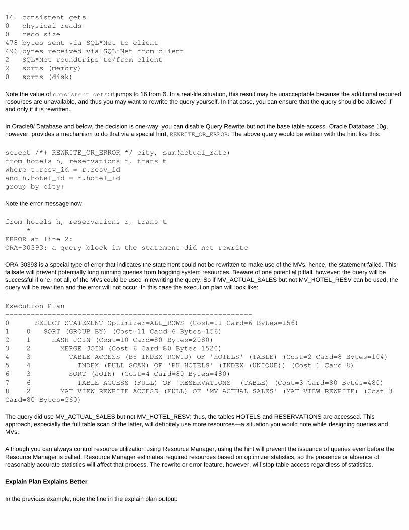
16 consistent gets0 physical reads0 redo size478 bytes sent via SQL*Net to client496 bytes received via SQL*Net from client2 SQL*Net roundtrips to/from client2 sorts (memory)0 sorts (disk)

Note the value of consistent gets: it jumps to 16 from 6. In a real-life situation, this result may be unacceptable because the additional required resources are unavailable, and thus you may want to rewrite the query yourself. In that case, you can ensure that the query should be allowed if and only if it is rewritten.

In Oracle9i Database and below, the decision is one-way: you can disable Query Rewrite but not the base table access. Oracle Database 10g, however, provides a mechanism to do that via a special hint, REWRITE_OR_ERROR. The above query would be written with the hint like this:

select /*+ REWRITE_OR_ERROR */ city, sum(actual_rate)from hotels h, reservations r, trans twhere t.resv_id = r.resv_idand h.hotel_id = r.hotel_idgroup by city;

Note the error message now.

from hotels h, reservations r, trans t *ERROR at line 2:ORA-30393: a query block in the statement did not rewrite

ORA-30393 is a special type of error that indicates the statement could not be rewritten to make use of the MVs; hence, the statement failed. This failsafe will prevent potentially long running queries from hogging system resources. Beware of one potential pitfall, however: the query will be successful if one, not all, of the MVs could be used in rewriting the query. So if MV_ACTUAL_SALES but not MV_HOTEL_RESV can be used, the query will be rewritten and the error will not occur. In this case the execution plan will look like:

Execution Plan----------------------------------------------------------0 SELECT STATEMENT Optimizer=ALL_ROWS (Cost=11 Card=6 Bytes=156)1 0 SORT (GROUP BY) (Cost=11 Card=6 Bytes=156)2 1 HASH JOIN (Cost=10 Card=80 Bytes=2080)3 2 MERGE JOIN (Cost=6 Card=80 Bytes=1520)4 3 TABLE ACCESS (BY INDEX ROWID) OF 'HOTELS' (TABLE) (Cost=2 Card=8 Bytes=104)5 4 INDEX (FULL SCAN) OF 'PK_HOTELS' (INDEX (UNIQUE)) (Cost=1 Card=8)6 3 SORT (JOIN) (Cost=4 Card=80 Bytes=480)7 6 TABLE ACCESS (FULL) OF 'RESERVATIONS' (TABLE) (Cost=3 Card=80 Bytes=480)8 2 MAT_VIEW REWRITE ACCESS (FULL) OF 'MV_ACTUAL_SALES' (MAT_VIEW REWRITE) (Cost=3 Card=80 Bytes=560)

The query did use MV_ACTUAL_SALES but not MV_HOTEL_RESV; thus, the tables HOTELS and RESERVATIONS are accessed. This approach, especially the full table scan of the latter, will definitely use more resources—a situation you would note while designing queries and MVs.

Although you can always control resource utilization using Resource Manager, using the hint will prevent the issuance of queries even before the Resource Manager is called. Resource Manager estimates required resources based on optimizer statistics, so the presence or absence of reasonably accurate statistics will affect that process. The rewrite or error feature, however, will stop table access regardless of statistics.

Explain Plan Explains Better

In the previous example, note the line in the explain plan output:

MAT_VIEW REWRITE ACCESS (FULL) OF 'MV_ACTUAL_SALES' (MAT_VIEW REWRITE)

This method of access—MAT_VIEW REWRITE—is new; it shows that the MV is being accessed, not the table or segment. This procedure immediately tells you if the table or MV is used, even if the names don't imply the nature of the segment.

Conclusion

Managing MVs is much easier in 10g with the introduction of the powerful new tuning advisors that can tell you a lot about the design of the MVs, taking the guesswork out of the picture. I especially like the tuning recommendations that can generate a complete script that can be implemented quickly, saving significant time and effort. The ability to force rewriting or abort the query can be very helpful in decision-support systems where resources must be conserved, and where a query that is not rewritten should not be allowed to run amuck inside the database.

For more information about managing MVs in 10g, see Chapter 8 of the Oracle Database Data Warehousing Guide 10g Release 1 (10.1).

Week 13Enterprise Manager 10g

Finally, a tool that serves as one-stop-shop for Oracle administration and management—whether by novices or experts

What tool do you use in your day-to-day DBA-related activities? It's a question I asked recently in a user group meeting.

The answers varied depending on the DBA's work experience. Most senior administrators expressed a preference for simple command-line SQL*Plus (my personal favorite), with the rest dividing their allegiances among a handful of third-party products. The same question, however, yielded a different response from entry-level DBAs: among that group, Enterprise Manager (EM) was clearly the tool of choice.

It's not hard to understand these preferences. Oracle Enterprise Manager has been steadily perfected since its introduction several years ago, beginning as the character-mode display SQL*DBA, evolving into a client OS-based tool, and finally taking on a Java flavor. The information presented by EM was sufficiently detailed for most DBA tasks, serving as a solution for users who were either too reluctant or too busy to learn a new syntax and wanted a GUI tool for managing common database chores such as adding users, modifying datafiles, and checking on rollback segments. The diagnostic pack supplied much-needed GUI support for performance tuning.

However, one of the major issues hampering EM's widespread adoption was its inability to keep pace with the development of the database server itself. For example, the Oracle9i Database version of EM doesn't support subpartitioning, a feature first introduced in Oracle8i.

The new version of EM in Oracle Database 10g changes that equation. It has a new architecture, a new interface, and most important, a very powerful and complete toolbox catering to all DBA skillsets—from novices to advanced users. And best of all, it's part of the installation itself without any additional cost. If you are evaluating third-party tools, you can certainly throw EM into the mix to light a fire under the competition. Even if you are an "in-command-line-we-trust" kind of DBA (like me), you will greatly appreciate how EM can help you in several situations.

In this installment I will introduce you to the new EM. Because the tool is so vast in scope, it will be impossible to cover the entire spectrum of features; instead, I will explain a few basics and offer pointers to additional material. Keeping in the spirit of this series, I will provide practical examples that demonstrate the use of the tool to solve real-life problems.

Architecture

EM 10g is installed by default when you install the 10g software. Conceptually, it differs from previous versions in that instead of being a client-installed tool, it's actually an HTTP server (called DB Console) sitting on the database server itself. (See Figure 1.) You can use any browser to see the EM interface.

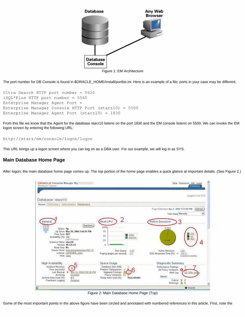
Figure 1: EM Architecture

The port number for DB Console is found in $ORACLE_HOME/install/portlist.ini. Here is an example of a file; ports in your case may be different.

Ultra Search HTTP port number = 5620iSQL*Plus HTTP port number = 5560Enterprise Manager Agent Port =Enterprise Manager Console HTTP Port (starz10) = 5500Enterprise Manager Agent Port (starz10) = 1830

From this file we know that the Agent for the database starz10 listens on the port 1830 and the EM console listens on 5500. We can invoke the EM logon screen by entering the following URL:

http://starz/em/console/logon/logon

This URL brings up a logon screen where you can log on as a DBA user. For our example, we will log in as SYS.

Main Database Home Page

After logon, the main database home page comes up. The top portion of the home page enables a quick glance at important details. (See Figure 2.)

Figure 2: Main Database Home Page (Top)

Some of the most important points in the above figure have been circled and annotated with numbered references in this article. First, note the

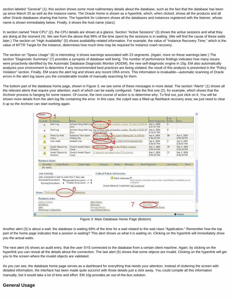
section labeled "General" (1); this section shows some most rudimentary details about the database, such as the fact that the database has been up since March 20 as well as the instance name. The Oracle Home is shown as a hyperlink, which, when clicked, shows all the products and all other Oracle databases sharing that home. The hyperlink for Listeners shows all the databases and instances registered with the listener, whose name is shown immediately below. Finally, it shows the host name (starz).

In section named "Host CPU" (2), the CPU details are shown at a glance. Section "Active Sessions" (3) shows the active sessions and what they are doing at the moment (4). We see from the above that 99% of the time spent by the sessions is in waiting. (We will find the cause of these waits later.) The section on "High Availability" (5) shows availability-related information. For example, the value of "Instance Recovery Time," which is the value of MTTR Target for the instance, determines how much time may be required for instance crash recovery.

The section on "Space Usage" (6) is interesting: it shows warnings associated with 23 segments. (Again, more on these warnings later.) The section "Diagnostic Summary" (7) provides a synopsis of database well being. The number of performance findings indicates how many issues were proactively identified by the Automatic Database Diagnostic Monitor (ADDM), the new self-diagnostic engine in 10g. EM also automatically analyzes your environment to determine if any recommended best practices are being violated; the result of this analysis is presented in the "Policy Violation" section. Finally, EM scans the alert log and shows any recent ORA errors. This information is invaluable—automatic scanning of Oracle errors in the alert log saves you the considerable trouble of manually searching for them.

The bottom part of the database home page, shown in Figure 3, we see some of these messages in more detail. The section "Alerts" (1) shows all the relevant alerts that require your attention, each of which can be easily configured. Take the first one (2), for example, which shows that the Archiver process is hanging for some reason. Of course, the next course of action is to determine why. To find out, just click on it. You will be shown more details from the alert.log file containing the error. In this case, the culprit was a filled-up flashback recovery area; we just need to clear it up so the Archiver can start working again.

Figure 3: Main Database Home Page (Bottom)

Another alert (3) is about a wait: the database is waiting 69% of the time for a wait related to the wait class "Application." Remember how the top part of the home page indicates that a session is waiting? This alert shows us what it is waiting on. Clicking on the hyperlink will immediately show you the actual waits.

The next alert (4) shows an audit entry, that the user SYS connected to the database from a certain client machine. Again, by clicking on the hyperlink you can reveal all the details about the connection. The last alert (5) shows that some objects are invalid. Clicking on the hyperlink will get you to the screen where the invalid objects are validated.

As you can see, the database home page serves as a dashboard for everything that needs your attention. Instead of cluttering the screen with detailed information, the interface has been made quite succinct with those details just a click away. You could compile all this information manually, but it would take a lot of time and effort. EM 10g provides an out-of-the-box solution.

General Usage

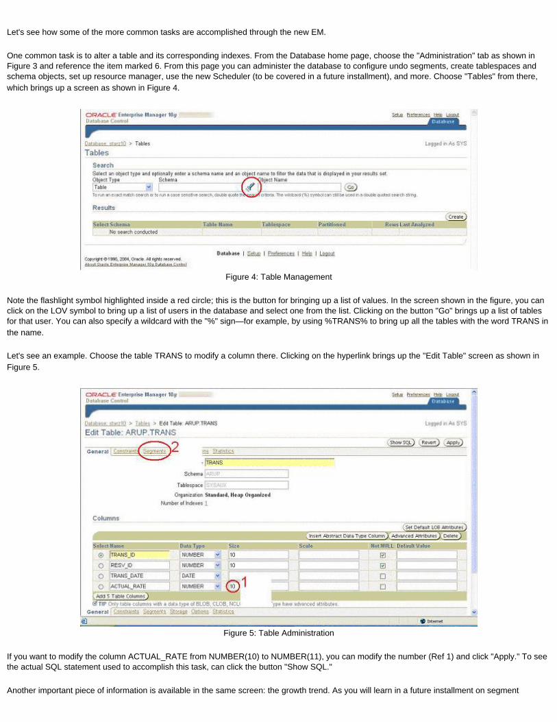
Let's see how some of the more common tasks are accomplished through the new EM.

One common task is to alter a table and its corresponding indexes. From the Database home page, choose the "Administration" tab as shown in Figure 3 and reference the item marked 6. From this page you can administer the database to configure undo segments, create tablespaces and schema objects, set up resource manager, use the new Scheduler (to be covered in a future installment), and more. Choose "Tables" from there, which brings up a screen as shown in Figure 4.

Figure 4: Table Management

Note the flashlight symbol highlighted inside a red circle; this is the button for bringing up a list of values. In the screen shown in the figure, you can click on the LOV symbol to bring up a list of users in the database and select one from the list. Clicking on the button "Go" brings up a list of tables for that user. You can also specify a wildcard with the "%" sign—for example, by using %TRANS% to bring up all the tables with the word TRANS in the name.

Let's see an example. Choose the table TRANS to modify a column there. Clicking on the hyperlink brings up the "Edit Table" screen as shown in Figure 5.

Figure 5: Table Administration

If you want to modify the column ACTUAL_RATE from NUMBER(10) to NUMBER(11), you can modify the number (Ref 1) and click "Apply." To see the actual SQL statement used to accomplish this task, can click the button "Show SQL."

Another important piece of information is available in the same screen: the growth trend. As you will learn in a future installment on segment

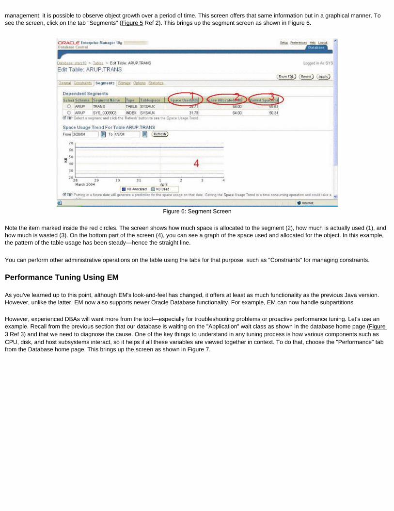
management, it is possible to observe object growth over a period of time. This screen offers that same information but in a graphical manner. To see the screen, click on the tab "Segments" (Figure 5 Ref 2). This brings up the segment screen as shown in Figure 6.

Figure 6: Segment Screen

Note the item marked inside the red circles. The screen shows how much space is allocated to the segment (2), how much is actually used (1), and how much is wasted (3). On the bottom part of the screen (4), you can see a graph of the space used and allocated for the object. In this example, the pattern of the table usage has been steady—hence the straight line.

You can perform other administrative operations on the table using the tabs for that purpose, such as "Constraints" for managing constraints.

Performance Tuning Using EM

As you've learned up to this point, although EM's look-and-feel has changed, it offers at least as much functionality as the previous Java version. However, unlike the latter, EM now also supports newer Oracle Database functionality. For example, EM can now handle subpartitions.

However, experienced DBAs will want more from the tool—especially for troubleshooting problems or proactive performance tuning. Let's use an example. Recall from the previous section that our database is waiting on the "Application" wait class as shown in the database home page (Figure 3 Ref 3) and that we need to diagnose the cause. One of the key things to understand in any tuning process is how various components such as CPU, disk, and host subsystems interact, so it helps if all these variables are viewed together in context. To do that, choose the "Performance" tab from the Database home page. This brings up the screen as shown in Figure 7.

Figure 7: Performance Tab

Note how all the metrics have been aligned on the same timeline, which makes viewing their interdependencies easier. Note the spike (3), which corresponds to the Scheduler task. It shows that some seven sessions were waiting for Scheduler-related waits at that time. So, what was the impact? Note the CPU metrics located in the same place (the green area)—they indicate the maximum CPU ever used, as shown in the graph by the broken line (4). Before and after that point, we don't see the CPU spikes occurring, which provides one clue. Note the spike in CPU run queue length (1), which is a direct consequence of the Scheduler, which might have generated an excessive memory requirement, having caused the increased paging activity (2). As you can see, all the symptoms fall in line to enable a better understanding of the database load "profile."

Note the spikes at the end of the timeline—increases in Run Queue Length (5) and Paging Rate (6)—which correlate to another spike in Physical Reads (7). What is the cause?

By comparing the graph "Sessions: Waiting and Working" with the time the spikes were occurring, we can see that most of the sessions were waiting on the "Application" wait class. But we need to find out exactly what it was waiting on during that time period. Click on the area at that time, which brings up the Active Sessions screen as shown in Figure 8.

Figure 8: Active Sessions Waits

The screen shows that the sessions were waiting for the wait event enq: TX – row lock contention. So what was the SQL statement that caused it? Simple: The SQL ID of the statement 8rkquk6u9fmd0 is shown on the screen itself (inside the red circle). Click on the SQL ID to bring up the SQL screen as shown in Figure 9.

Figure 9: SQL Details

On this screen you can see the SQL statement and relevant details about it, including the execution plan. It turns out that this SQL was causing row lock contention, so application design may be a source of the problem.

Latch Contention

Suppose that clicking on the "Performance" tab takes you to a screen similar to that shown in Figure 10.

Figure 10: Performance Tab, Example 2

In the figure, note the metrics highlighted inside the red rectangle. You can see a lot of CPU-related waits around 12:20AM, which resulted in a large run queue in the CPU. We need to diagnose this wait.

First, click on the graph on the area shown for CPU contention (marked with "Click Here" on the figure) to see that particular wait in detail, shown in Figure 11.

Figure 11: Active Session Waits

Note the shaded box in the "Active Sessions Working: CPU Used" graph (1). You can drag it using the mouse to place the focus. This operation causes the pie charts below (2 and 3) to be calculated only within the timeframe contained in that box. From there we see that a specific SQL with id 8ggw94h7mvxd7 is working extra hard (2). We also see that the user session with username ARUP and SID 265 is a top worker (3). Click on the session to see the details. This operation brings up a "Session Details" screen. Click on the tab "Wait Events" to bring up the details of the wait events experienced by the session, similar to what you see in Figure 12.

Figure 12: Wait Event Details

In this screen, note the longest wait of 118 centiseconds, highlighted inside a red circle, which is waiting for a library cache. When you click on the hyperlink for "Latch: Library Cache," you will see a screen similar to that in Figure 13.

Figure 13: Wait Histogram

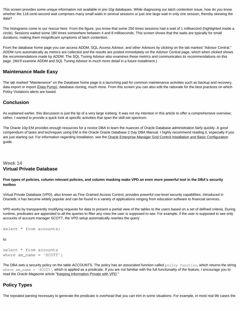
This screen provides some unique information not available in pre-10g databases. While diagnosing our latch contention issue, how do you know whether the 118 centi-second wait comprises many small waits in several sessions or just one large wait in only one session, thereby skewing the data?

The histograms come to our rescue here. From the figure, you know that some 250 times sessions had a wait of 1 millisecond (highlighted inside a circle). Sessions waited some 180 times somewhere between 4 and 8 milliseconds. This screen shows that the waits are typically for small durations, making them insignificant symptoms of latch contention.

From the database home page you can access ADDM, SQL Access Advisor, and other Advisors by clicking on the tab marked "Advisor Central." ADDM runs automatically as metrics are collected and the results are posted immediately on the Advisor Central page, which when clicked shows the recommendations made by ADDM. The SQL Tuning Advisor also examines these metrics and communicates its recommendations on this page. (We'll examine ADDM and SQL Tuning Advisor in much more detail in a future installment.)

Maintenance Made Easy

The tab marked "Maintenance" on the Database home page is a launching pad for common maintenance activities such as backup and recovery, data export or import (Data Pump), database cloning, much more. From this screen you can also edit the rationale for the best practices on which Policy Violations alerts are based.

Conclusion

As explained earlier, this discussion is just the tip of a very large iceberg. It was not my intention in this article to offer a comprehensive overview; rather, I wanted to provide a quick look at specific activities that span the skill-set spectrum.

The Oracle 10g EM provides enough resources for a novice DBA to learn the nuances of Oracle Database administration fairly quickly. A good compendium of tasks and techniques using EM is the Oracle Oracle Database 2 Day DBA Manual. I highly recommend reading it, especially if you are just starting out. For information regarding installation, see the Oracle Enterprise Manager Grid Control Installation and Basic Configuration guide.

Week 14Virtual Private Database

Five types of policies, column relevant policies, and column masking make VPD an even more powerful tool in the DBA's security toolbox

Virtual Private Database (VPD), also known as Fine Grained Access Control, provides powerful row-level security capabilities. Introduced in Oracle8i, it has become widely popular and can be found in a variety of applications ranging from education software to financial services.

VPD works by transparently modifying requests for data to present a partial view of the tables to the users based on a set of defined criteria. During runtime, predicates are appended to all the queries to filter any rows the user is supposed to see. For example, if the user is supposed to see only accounts of account manager SCOTT, the VPD setup automatically rewrites the query:

select * from accounts;

to:

select * from accountswhere am_name = 'SCOTT';

The DBA sets a security policy on the table ACCOUNTS. The policy has an associated function called policy function, which returns the string where am_name = 'SCOTT', which is applied as a predicate. If you are not familiar with the full functionality of the feature, I encourage you to read the Oracle Magazine article "Keeping Information Private with VPD."

Policy Types

The repeated parsing necessary to generate the predicate is overhead that you can trim in some situations. For example, in most real life cases the

predicate is not as static as where am_name = 'SCOTT'; it's probably more dynamic based on who the user is, the authority level of the user, which account manager she reports to, and so on. The string created and returned by the policy function may become very dynamic, and to guarantee the outcome, Oracle must re-execute the policy function every time, wasting resources and reducing performance. This type of policy, where the predicate can potentially be very different each time it is executed, is known as a "dynamic" policy, and has been available in Oracle9i Database and prior releases..

In addition to retaining dynamic policy, Oracle Database 10g introduces several new types of policies based on how the predicate is constructed providing better controls for improving performance: context_sensitive, shared_context_sensitive, shared_static, and static. Now, let's what each policy type means and how to use it in appropriate situations.

Dynamic Policy. To retain backward compatibility, the default policy type in 10g is "dynamic"—just as it was in Oracle9i. In this case, the policy function is re-evaluated each time the table is accessed, for each row and for every user. Let's examine the policy predicate closely:

where am_name = 'SCOTT'

Ignoring the where clause, the predicate has two distinct parts: the portion before the equality operator (am_name) and the one after it ('SCOTT'). In most cases, the one after is more like a variable in that it is supplied from the user's data (if the user is SCOTT, the value would be 'SCOTT'.) The part before the equality sign is static. So, even though the function does have to evaluate the policy function for each row to generate the appropriate predicate, the knowledge about the static-ness of the before-part and dynamic-ness of the after-part can be used to improve performance. This approach is possible in 10g using a policy of type "context_sensitive" as a parameter in the dbms_rls.add_policy call:

policy_type => dbms_rls.context_sensitive

In another example scenario, we have a table called ACCOUNTS with several columns, one of which is BALANCE, indicating the account balance. Let's assume that a user is allowed to view accounts below a certain balance that is determined by an application context. Instead of hard-coding this balance amount in a policy function, we can use an application context as in:

create or replace vpd_pol_func( p_schema in varchar2, p_table in varchar2) return varchar2isbegin return 'balance < sys_context(''vpdctx'', ''maxbal'')';end;

The attribute MAXBAL of the application context VPDCTX can be set earlier in the session and the function can simply get the value at the runtime.

Note the example carefully here. The predicate has two parts: the one before the less-than sign and the other after it. The one before, the word "balance," is a literal. The one after is more or less static because the application context variable is constant until it is changed. If the application context attribute does not change, the entire predicate is constant, and hence the function need not be re-executed. Oracle Database 10g recognizes this fact for optimization if the policy type is defined as context sensitive. If no session context changes have occurred in the session, the function is not re-executed, significantly improving performance.

Static Policy. Sometimes a business operation may warrant a predicate that is more static. For instance, in the context-sensitive policy type example, we defined the maximum balance seen by a user as a variable. This approach is useful in the case of web applications where an Oracle userid is shared by many web users and based on their authority this variable (application context) is set by the application. Therefore web users TAO and KARTHIK, both connecting to the database as user APPUSER, may have two different values of the application context in their session. Here the value of MAXBAL is not tied to the Oracle userid, but rather to the individual session of TAO and KARTHIK.

In the static policy case the predicate is more predictable, as described below.

LORA and MICHELLE are account managers for Acme Bearings and Goldtone Bearings respectively. When they connect to the database, they use their own id and should only see the rows pertaining to them. In Lora's case, the predicate becomes where CUST_NAME = 'ACME'; for Michelle, where CUST_NAME = 'GOLDTONE'. Here the predicate is tied to their userids, and hence any session they create will always have the same value in the application context.

This fact can be exploited by 10g to cache the predicate in the SGA and reuse that in the session without ever re-executing the policy function. The

policy function looks like this:

create or replace vpd_pol_func( p_schema in varchar2, p_table in varchar2) return varchar2isbegin return 'cust_name = sys_context(''vpdctx'', ''cust_name'')';end;

And the policy is defined as:

policy_type => dbms_rls.static

This approach ensures that the policy function is executed only once. Even if the application contexts are changed in the session, the function is never re-executed, making this process extremely fast.

Static policies are recommended for hosting your applications across several subscribers. In this case a single database has data for several users or subscribers. When each subscriber logs in, an after-logon trigger can set the application context to a value that is used in the policy function to very quickly generate a predicate.

However, defining a policy as static is also a double-edged sword. In the above example, we assumed that the value of the application context attribute VPDCTX.CUST_NAME does not change inside a session. What if that assumption is incorrect? If the value changes, the policy function will not be executed and therefore the new value will not be used in the predicate, returning wrong results! So, be very careful in defining a policy as static; you must be absolutely certain that the value will not change. If you can't make that assumption, better to define the policy as context sensitive instead.

Shared Policy Types. To reuse code and maximize the usage of parsed code, you might decide to use a common policy function for several tables. For instance, in the above example, we may have different tables for different types of accounts—SAVINGS and CHECKING—but the rule is still the same: users are restricted from seeing accounts with balances more than they are authorized for. This scenario calls for a single function used for policies on CHECKING and SAVINGS tables. The policy is created as context_sensitive.

Suppose this is the sequence of events:

1. Session connected2. Application context is set3. select * from savings;4. select * from checking;

Even though the application context does not change between steps 3 and 4, the policy function will be re-executed, simply because the tables selected are different now. This is not desirable, as the policy function is the same and there is no need to re-execute the function.

New in 10g is the ability to share a policy across objects. In the above example, you would define the policy type of these policies as:

policy_type => dbms_rls.shared_context_sensitive

Declaring the policies as "shared" improves performance by not executing the function again in the cases as shown above.

Selective Columns

Now imagine a situation where the VPD policy should be applied only if certain columns are selected. In the above example with table ACCOUNTS, the rows are as follows:

ACCTNO ACCT_NAME BALANCE------ ------------ ------- 1 BILL CAMP 1000

2 TOM CONNOPHY 2000 3 ISRAEL D 1500

Michelle is not supposed to see accounts with balances over 1,600. When she issues a query like the following:

select * from accounts;

she sees:

ACCTNO ACCT_NAME BALANCE------ ------------ ------- 1 BILL CAMP 1000 3 ISRAEL D 1500

acctno 2, with balance more than 1,600, has been suppressed in the display. As far as Michelle is concerned, there are only two rows in the table, not three. When she issues a query such as:

select count(*) from accounts;

which simply counts the number of records from the table, the output is two, not three.

However, here we may decide to relax the security policy a bit. In this query Michelle can't view confidential data such as account balance; she merely counts all the records in the table. Consistent with the security policy, we may allow this query to count all the records whether or not she is allowed to see them. If this is the requirement, another parameter in the call to dbms_rls.add_policy in 10g allows that function:

sec_relevant_cols => 'BALANCE'

Now when the user selects the column BALANCE, either explicitly or implicitly as in select *, the VPD policy will kick in to restrict the rows. Otherwise all rows of the table will be selected, as in the query where the user has selected only the count of the total rows, not the column BALANCE. If the above parameter is set as shown, then the query

select count(*) from accounts;

will show three columns, not two. But the query:

select * from accounts;

will still return only two records, as expected.

Column Masking

Now let's add more requirements to our current example. Instead of suppressing the display of rows with a balance above the threshold, we may want to show all the rows while masking the balance column where the value is above the threshold. The security-relevant column is still BALANCE.

Michelle is not supposed to see accounts with balances over 1,600. When she issues a query like the following:

select * from accounts;

she would have seen only two rows, acctnos 1 and 3. But, instead, we may want her to see:

ACCTNO ACCT_NAME BALANCE------ ------------ ------- 1 BILL CAMP 1000 2 TOM CONNOPHY <null> 3 ISRAEL D 1500

Note how all the rows are displayed but the value of the column BALANCE is shown as null (displayed as <null>) for acctno 2, where the balance is actually 2,000, more than the threshold of 1,600. This approach is called "column masking," and is enabled by specifying the parameter in the call to dbms_rls.add_policy:

sec_relevant_cols_opt => dbms_rls.all_rows

This tactic can be very useful in cases where only values of certain columns are important, and requires no complicated custom code. It is also a great alternative to requiring stored data encryption.

Conclusion

In Oracle Database 10g, VPD has grown into a very powerful feature with the ability to support a variety of requirements, such as masking columns selectively based on the policy and applying the policy only when certain columns are accessed. The performance of the policy can also be increased through multiple types of policy by exploiting the nature of the application, making the feature applicable to multiple situations.

For more information about VPD and the dbms_rls package, consult Chapter 79 of PL/SQL Packages and Types Reference and the Oracle Database Security Guide. You can also read the book I coauthored with Don Burleson on the subject, Oracle Privacy Security Auditing (Rampant TechPress).

Week 15Segment Management

Manage storage in segments efficiently with Oracle Database 10g—by reclaiming wasted space, reorganizing tables online, and estimating growth trends

Recently, I was asked to evaluate an RDBMS that competes with Oracle Database. During the vendor's presentation, the feature that registered the biggest "wow" factor in the audience was its support for online reorganizations—the product can relocate data blocks to make the equivalent of segments more compact online, without affecting current users.

At that time, Oracle did not offer such a capability in Oracle9i Database. But now, with Oracle Database 10g, you can easily reclaim wasted space and compact objects online—just for starters.

Before examining the feature, however, let's take a look at the "traditional" approach to this task.

Current Practices

Consider a segment, such as a table, where the blocks are filled up as shown in Figure 1. During normal operation, some rows are deleted, as shown in Figure 2. Now we have a lot of wasted space: (i) between the previous end of the table and the existing block and (ii) inside the blocks where some of the rows have not been deleted.

Figure 1: The blocks allocated to the table. Rows are indicated by grey squares.

Oracle does not release that space for use by other objects for a simple reason: because that space is reserved for new inserts and to accommodate the growth of existing rows. The highest space occupied is known as a High Water Mark (HWM), as shown in Figure 2.

Figure 2: The blocks after rows have been deleted; the HWM remains unchanged.

There are two main problems with this approach, however:

● When a user issues a full table scan, Oracle must scan the segment all the way up to the HWM, even though it does not find anything. This task extends full table scan time.

● When rows are inserted with direct path—for example, through Direct Load Insert (insert with the APPEND hint) or through the SQL*Loader direct path—the data blocks are placed directly above the HWM. The space below it remains wasted.

In Oracle9i and below, you can reclaim space by dropping the table, recreating it, and then reloading the data; or by moving the table to a different tablespace using the ALTER TABLE MOVE command. Both these processes must occur offline. Alternatively, you can use the online table reorganization feature, but that requires at least double the space of the existing table.

In 10g, this task has become trivial; you can now shrink segments, tables, and indexes to reclaim free blocks and give them to the database for other uses, provided that Automatic Segment Space Management (ASSM) is enabled in your tablespace. Let's see how.

Segment Management the 10g Way

Suppose you have a table BOOKINGS, which holds online bookings from the website. After the booking is confirmed, it's stored in an archival table BOOKINGS_HIST and the row is deleted from BOOKINGS. The time between booking and confirmation varies widely among customers, so a lot of rows are inserted above the HWM of the table because sufficient space is not available from the deleted rows.

Now you need to reclaim wasted space. First, find out exactly how much space is wasted in that segment that can be reclaimed. Because this is in an ASSM-enabled tablespace, you have to use the procedure SPACE_USAGE of the package DBMS_SPACE, as shown below.

declare

l_fs1_bytes number; l_fs2_bytes number; l_fs3_bytes number; l_fs4_bytes number; l_fs1_blocks number; l_fs2_blocks number; l_fs3_blocks number; l_fs4_blocks number; l_full_bytes number; l_full_blocks number; l_unformatted_bytes number; l_unformatted_blocks number;begin dbms_space.space_usage( segment_owner => user, segment_name => 'BOOKINGS', segment_type => 'TABLE', fs1_bytes => l_fs1_bytes, fs1_blocks => l_fs1_blocks, fs2_bytes => l_fs2_bytes, fs2_blocks => l_fs2_blocks, fs3_bytes => l_fs3_bytes, fs3_blocks => l_fs3_blocks, fs4_bytes => l_fs4_bytes, fs4_blocks => l_fs4_blocks, full_bytes => l_full_bytes, full_blocks => l_full_blocks, unformatted_blocks => l_unformatted_blocks, unformatted_bytes => l_unformatted_bytes ); dbms_output.put_line(' FS1 Blocks = '||l_fs1_blocks||' Bytes = '||l_fs1_bytes); dbms_output.put_line(' FS2 Blocks = '||l_fs2_blocks||' Bytes = '||l_fs2_bytes); dbms_output.put_line(' FS3 Blocks = '||l_fs3_blocks||' Bytes = '||l_fs3_bytes); dbms_output.put_line(' FS4 Blocks = '||l_fs4_blocks||' Bytes = '||l_fs4_bytes); dbms_output.put_line('Full Blocks = '||l_full_blocks||' Bytes = '||l_full_bytes);end;/The output is:FS1 Blocks = 0 Bytes = 0

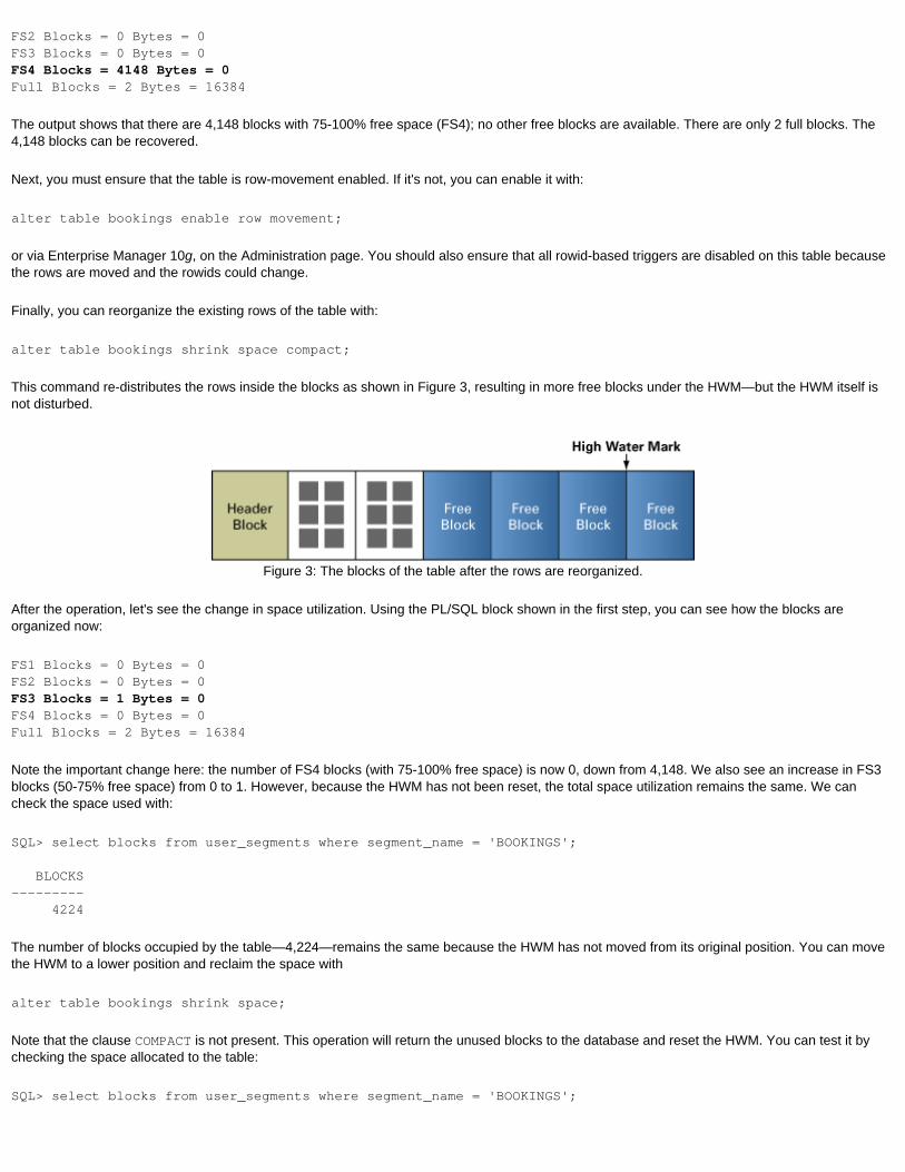
FS2 Blocks = 0 Bytes = 0FS3 Blocks = 0 Bytes = 0FS4 Blocks = 4148 Bytes = 0Full Blocks = 2 Bytes = 16384

The output shows that there are 4,148 blocks with 75-100% free space (FS4); no other free blocks are available. There are only 2 full blocks. The 4,148 blocks can be recovered.

Next, you must ensure that the table is row-movement enabled. If it's not, you can enable it with:

alter table bookings enable row movement;

or via Enterprise Manager 10g, on the Administration page. You should also ensure that all rowid-based triggers are disabled on this table because the rows are moved and the rowids could change.

Finally, you can reorganize the existing rows of the table with:

alter table bookings shrink space compact;

This command re-distributes the rows inside the blocks as shown in Figure 3, resulting in more free blocks under the HWM—but the HWM itself is not disturbed.

Figure 3: The blocks of the table after the rows are reorganized.

After the operation, let's see the change in space utilization. Using the PL/SQL block shown in the first step, you can see how the blocks are organized now:

FS1 Blocks = 0 Bytes = 0FS2 Blocks = 0 Bytes = 0FS3 Blocks = 1 Bytes = 0FS4 Blocks = 0 Bytes = 0Full Blocks = 2 Bytes = 16384

Note the important change here: the number of FS4 blocks (with 75-100% free space) is now 0, down from 4,148. We also see an increase in FS3 blocks (50-75% free space) from 0 to 1. However, because the HWM has not been reset, the total space utilization remains the same. We can check the space used with:

SQL> select blocks from user_segments where segment_name = 'BOOKINGS';

BLOCKS--------- 4224

The number of blocks occupied by the table—4,224—remains the same because the HWM has not moved from its original position. You can move the HWM to a lower position and reclaim the space with

alter table bookings shrink space;

Note that the clause COMPACT is not present. This operation will return the unused blocks to the database and reset the HWM. You can test it by checking the space allocated to the table:

SQL> select blocks from user_segments where segment_name = 'BOOKINGS';

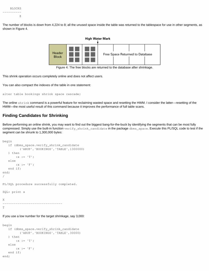
BLOCKS---------- 8

The number of blocks is down from 4,224 to 8; all the unused space inside the table was returned to the tablespace for use in other segments, as shown in Figure 4.

Figure 4: The free blocks are returned to the database after shrinkage.

This shrink operation occurs completely online and does not affect users.

You can also compact the indexes of the table in one statement:

alter table bookings shrink space cascade;

The online shrink command is a powerful feature for reclaiming wasted space and resetting the HWM. I consider the latter—resetting of the HWM—the most useful result of this command because it improves the performance of full table scans.

Finding Candidates for Shrinking

Before performing an online shrink, you may want to find out the biggest bang-for-the-buck by identifying the segments that can be most fully compressed. Simply use the built-in function verify_shrink_candidate in the package dbms_space. Execute this PL/SQL code to test if the segment can be shrunk to 1,300,000 bytes:

begin if (dbms_space.verify_shrink_candidate ('ARUP','BOOKINGS','TABLE',1300000) ) then :x := 'T'; else :x := 'F'; end if;end;/

PL/SQL procedure successfully completed.

SQL> print x

X--------------------------------T

If you use a low number for the target shrinkage, say 3,000:

begin if (dbms_space.verify_shrink_candidate ('ARUP','BOOKINGS','TABLE',30000) ) then :x := 'T'; else :x := 'F'; end if;end;

the value of the variable x is set to 'F', meaning the table cannot be shrunk to 3,000 bytes.

Taking the Guesswork Out of Index Space Requirements

Now let's say you are about to embark on the task of creating an index on a table, or perhaps a set of tables. Besides the usual structural elements such as columns and uniqueness, the most important thing you have to consider is the expected size of the index—you must ensure that the tablespace has enough space to hold the new index.

With Oracle9i Database and below, many DBAs use tools ranging from spreadsheets to standalone programs to estimate the size of the future index. In 10g, this task has become extremely trivial through the use of the DBMS_SPACE package. Let's see it in action.

We are asked to create an index on the columns booking_id and cust_name of the table BOOKINGS. How much space does the proposed index need? All you do is execute the following PL/SQL script.

declare l_used_bytes number; l_alloc_bytes number;begin dbms_space.create_index_cost ( ddl => 'create index in_bookings_hist_01 on bookings_hist '|| '(booking_id, cust_name) tablespace users', used_bytes => l_used_bytes, alloc_bytes => l_alloc_bytes ); dbms_output.put_line ('Used Bytes = '||l_used_bytes); dbms_output.put_line ('Allocated Bytes = '||l_alloc_bytes);end;/

The output is:

Used Bytes = 7501128Allocated Bytes = 12582912

Suppose you want to use some parameters that will potentially increase the size of the index—for example, specifying an INITRANS parameter of 10.

declare l_used_bytes number; l_alloc_bytes number;begin dbms_space.create_index_cost ( ddl => 'create index in_bookings_hist_01 on bookings_hist '|| '(booking_id, cust_name) tablespace users initrans 10', used_bytes => l_used_bytes, alloc_bytes => l_alloc_bytes ); dbms_output.put_line ('Used Bytes = '||l_used_bytes); dbms_output.put_line ('Allocated Bytes = '||l_alloc_bytes);end;/

The output is:

Used Bytes = 7501128Allocated Bytes = 13631488

Note the increase in the allocated bytes from specifying a higher INITRANS. Using this approach you can easily determine the impact of the index on storage space.

You should be aware of two important caveats, however. First, this process applies only to tablespaces with SEGMENT SPACE MANAGEMENT AUTO

turned on. Second, the package calculates the estimated size of the index from the statistics on the table. Hence it's very important to have relatively fresh statistics on the tables. But beware: the absence of statistics on the table will not result in an error in the use of the package, but will yield a wrong result.

Estimating Table Size

Suppose there is a table named BOOKINGS_HIST, which has the average row length of 30,000 rows and the PCTFREE parameter of 20. What if you wanted to increase the parameter PCT_FREE to 3—by what amount will the table increase in size? Because 30 is a 10% increase over 20, will the size go up by 10%? Instead of asking your psychic, ask the procedure CREATE_TABLE_COST inside the package DBMS_SPACE. Here is how you can estimate the size:

declare l_used_bytes number; l_alloc_bytes number;begin dbms_space.create_table_cost ( tablespace_name => 'USERS', avg_row_size => 30, row_count => 30000, pct_free => 20, used_bytes => l_used_bytes, alloc_bytes => l_alloc_bytes ); dbms_output.put_line('Used: '||l_used_bytes); dbms_output.put_line('Allocated: '||l_alloc_bytes);end;/

The output is:

Used: 1261568Allocated: 2097152

Changing the table's PCT_FREE parameter to 30 from 20, by specifying

pct_free => 30

we get the output:

Used: 1441792Allocated: 2097152

Note how the used space has increased from 1,261,568 to 1,441,792 because the PCT_FREE parameter conserves less room in the data block for user data. The increase is about 14%, not 10%, as expected. Using this package you can easily calculate the impact of parameters such as PCT_FREE on the size of the table, or of moving the table to a different tablespace.

Predicting the Growth of a Segment

It's holiday weekend and Acme Hotels is expecting a surge in demand. As a DBA, you are trying to understand the demand so that you can ensure there is enough space available. How do you predict the space utilization of the table?

Just ask 10g; you will be surprised how accurately and intelligently it can make that prediction for you. You simply issue this query:

select * from table(dbms_space.OBJECT_GROWTH_TREND ('ARUP','BOOKINGS','TABLE'));

The function dbms_space.object_growth_trend() returns record in PIPELINEd format, which can be displayed by the TABLE() casting. Here is the output:

TIMEPOINT SPACE_USAGE SPACE_ALLOC QUALITY

------------------------------ ----------- ----------- ------------05-MAR-04 08.51.24.421081 PM 8586959 39124992 INTERPOLATED06-MAR-04 08.51.24.421081 PM 8586959 39124992 INTERPOLATED07-MAR-04 08.51.24.421081 PM 8586959 39124992 INTERPOLATED08-MAR-04 08.51.24.421081 PM 126190859 1033483971 INTERPOLATED09-MAR-04 08.51.24.421081 PM 4517094 4587520 GOOD10-MAR-04 08.51.24.421081 PM 127469413 1044292813 PROJECTED11-MAR-04 08.51.24.421081 PM 128108689 1049697234 PROJECTED12-MAR-04 08.51.24.421081 PM 128747966 1055101654 PROJECTED13-MAR-04 08.51.24.421081 PM 129387243 1060506075 PROJECTED14-MAR-04 08.51.24.421081 PM 130026520 1065910496 PROJECTED

The output clearly shows the size of the table BOOKINGS at various times as shown in the column TIMEPOINT, in the TIMESTAMP datatype. The SPACE_ALLOC column shows the bytes allocated to the table and the SPACE_USAGE column shows how many of those bytes have been used. This information is collected by the Automatic Workload Repository, or AWR (see Week 6 of this series), every day. In the above output, the data was collected well on March 9, 2004, as indicated by the value of the column QUALITY - "GOOD." The space allocated and usage figures are accurate for that day. However, for all subsequent days, the value of this column is PROJECTED, indicating that the space calculations are projected from the data collected by the AWR facility—not collected directly from the segment.

Note the values in this column prior to March 9—they are all INTERPOLATED. In other words, the value was not really collected or projected, but simply interpolated from the usage pattern for whatever data is available. Most likely the data was not available at that time and hence the values had to be interpolated.

Conclusion

With the availability of segment level manipulations you now have fine-grained control over how space is used inside a segment, which can be exploited to reclaim free space inside a table, reorganize the table rows to make it more compact online, and much more. These facilities help DBAs free themselves from the routine and mundane tasks like table reorganization. The online segment shrink feature is especially helpful in eliminating internal fragmentation and lowering the high water mark of the segment, which can significantly reduce the cost of a full table scan.

For more information about the SHRINK operation, see this section of the Oracle Database SQL Reference. Learn more about the DBMS_SPACE package in Chapter 88 of the PL/SQL Packages and Types Reference. For a comprehensive review of all new space management features in Oracle Database 10g, read the Technical Whitepaper The Self-Managing Database: Proactive Space & Schema Object Management. Finally, a demo of Oracle Database 10g space management is available online.

Week 16Transportable Tablespaces

Transportable tablespaces are now portable across platforms, making data publication quicker and easier. Plus, external table downloads make the task of data movement with transformation simpler and faster.

How do you move data from one database to another? Of the several methods, one in particular stands out: transportable tablespaces. In this approach, you take a set of self-contained, read-only tablespaces, export only the metadata, copy the datafiles of those tablespaces at the OS level to the target platform, and import the metadata into the data dictionary—a process known as plugging.

OS file copy is generally much faster than other traditional means of data movement such as export/import or SQL*Loader. However, in Oracle9i Database and below, a restriction limits its usefulness to only a few cases in which both the target and source database run on the same OS platform—you can't transport tablespaces between Solaris and HP-UX, for example.

In Oracle Database 10g, this restriction has disappeared: you can now transport tablespaces between platforms as long as the OS byte orders are identical. A lengthy discussion of byte order is beyond our boundaries here, but suffice it to say that some operating systems, including Windows, store multi-byte binary data with the least significant byte in the lowest memory address; therefore, the system is called little endian. Conversely, other OSs, including Solaris, store the most significant byte in the lowest memory address, hence the term big endian. When a big-endian system tries to read data from a little-endian one, a conversion process is required—otherwise, the byte order will lead to an incorrect interpretation of the read data. (For a detailed explanation of byte order, read the excellent article "Introduction to Endianness" from the Jan. 2002 issue of Embedded Systems Programming.) When transporting tablespaces between platforms of same endianess, however, no conversion is required.

How do you know which operating systems follow which byte order? Instead of guessing or having to search the internet, simply issue the query:

SQL> select * from v$transportable_platform order by platform_id;

PLATFORM_ID PLATFORM_NAME ENDIAN_FORMAT----------- ----------------------------------- -------------- 1 Solaris[tm] OE (32-bit) Big 2 Solaris[tm] OE (64-bit) Big 3 HP-UX (64-bit) Big 4 HP-UX IA (64-bit) Big 5 HP Tru64 UNIX Little 6 AIX-Based Systems (64-bit) Big 7 Microsoft Windows IA (32-bit) Little 8 Microsoft Windows IA (64-bit) Little 9 IBM zSeries Based Linux Big 10 Linux IA (32-bit) Little 11 Linux IA (64-bit) Little 12 Microsoft Windows 64-bit for AMD Little 13 Linux 64-bit for AMD Little 15 HP Open VMS Little 16 Apple Mac OS Big

Suppose you want to transport a tablespace USERS from a host machine SRC1, running Linux on Intel Architecture to machine TGT1, running Microsoft Windows. Both the source and target platforms are of little endian type. The datafile for the tablespace USERS is users_01.dbf. You would follow an approach similar to the following.

1. Make the tablespace READ ONLY:

alter tablespace users read only;

2. Export the tablespace. From the OS prompt, issue:

exp tablespaces=users transport_tablespace=y file=exp_ts_users.dmp

The file exp_ts_users.dmp contains only metadata—not the contents of the tablespace USERS—so it will be very small.

3. Copy the files exp_ts_users.dmp and users_01.dbf to the host TGT1. If you were using FTP, you would specify the binary option.4. Plug the tablespace into the database. From the OS command prompt, you would issue:

imp tablespaces=users transport_tablespace=y file=exp_ts_users.dmp datafiles='users_01.dbf'

After Step 4, the target database will have a tablespace named USERS and the contents of the tablespace will be available.

Remember, the systems SRC1 and TGT1 are Linux and Windows respectively. As of Oracle9i, databases running on TGT1 will not recognize the datafile users_01.dbf in Step 4, rendering this whole process useless. You would have to resort to some other approach such as regular export and import, creating a flat file and loading via SQL*Loader, or direct load insert across database links.

In 10g, these alternatives are unnecessary because the target database will recognize a datafile from another platform. In our example, the byte order of the OSs on which the source and target hosts run are the same (little endian), so no conversion is needed.

This capability is particularly useful in data warehouses where smaller, subject-oriented data marts are often populated from the warehouse after a refresh. With 10g, these data marts can now be placed in smaller, cheaper machines, such as Intel boxes running Linux, with the data warehouse server on a larger enterprise-class machine. In essence, with transportable tablespaces, you can now make better use of various hardware and OS mixes.

Across Differing Endianness of Platforms

If the platforms are of different endianness, how will you achieve transferability? As I explained earlier, the byte order of the target machine, if different than the source, will read the data file incorrectly, making the mere copying of the data files impossible. But don't lose heart; help is available from the Oracle 10g RMAN utility, which supports the conversion of datafiles from one byte order to another.

In the above example, if the host SRC1 runs on Linux (little endian) and the target host TGT1 runs on HP-UX (big endian), you need to introduce another step between Steps 3 and 4 for conversion. Using RMAN, you would convert the datafile from Linux to HP-UX format on the source

machine SRC1 (assuming you have made the tablespace read only):

RMAN> convert tablespace users2> to platform 'HP-UX (64-bit)'3> format='/home/oracle/rman_bkups/%N_%f';

Starting backup at 14-MAR-04using channel ORA_DISK_1channel ORA_DISK_1: starting datafile conversioninput datafile fno=00004 name=/usr/oradata/dw/starz10/users01.dbfconverted datafile=/home/oracle/rman_bkups/USERS_4channel ORA_DISK_1: datafile conversion complete, elapsed time: 00:00:07Finished backup at 14-MAR-04

This step produces a file in the standard RMAN file format <tablespace_name>_<absolute_datafile_no> in the directory /home/oracle/rman_bkups. Note that the datafile for tablespace USERS is not touched; rather, a new file is created for HP-UX. Now this file can be copied over to the target system, and the rest of the steps are easy.

This RMAN conversion command is quit powerful. In the form given above, it can create the datafiles in sequence. For a tablespace containing multiple datafiles, you can instruct conversion to run in parallel. To do so, you would add a clause to the above command:

parallelism = 4

which creates four RMAN channels, with each one working on a datafile. However, a more useful approach is to convert a large number of tablespaces in one step, which is where parallelism can really help. Here we are converting two tablespaces, USERS and MAINTS, to HP-UX:

RMAN> convert tablespace users, maints2> to platform 'HP-UX (64-bit)'3> format='/home/oracle/rman_bkups/%N_%f'4> parallelism = 5;

Starting backup at 14-MAR-04using target database controlfile instead of recovery catalogallocated channel: ORA_DISK_1channel ORA_DISK_1: sid=244 devtype=DISKallocated channel: ORA_DISK_2channel ORA_DISK_2: sid=243 devtype=DISKallocated channel: ORA_DISK_3channel ORA_DISK_3: sid=245 devtype=DISKallocated channel: ORA_DISK_4channel ORA_DISK_4: sid=272 devtype=DISKallocated channel: ORA_DISK_5channel ORA_DISK_5: sid=253 devtype=DISKchannel ORA_DISK_1: starting datafile conversioninput datafile fno=00004 name=/usr/oradata/dw10/dw10/users01.dbfchannel ORA_DISK_2: starting datafile conversioninput datafile fno=00005 name=/usr/oradata/dw10/dw10/users02.dbfchannel ORA_DISK_3: starting datafile conversioninput datafile fno=00006 name=/usr/oradata/dw10/dw10/maints01.dbfchannel ORA_DISK_4: starting datafile conversioninput datafile fno=00007 name=/usr/oradata/dw10/dw10/maints02.dbfconverted datafile=/home/oracle/rman_bkups/USERS_4channel ORA_DISK_1: datafile conversion complete, elapsed time: 00:00:03converted datafile=/home/oracle/rman_bkups/USERS_5channel ORA_DISK_2: datafile conversion complete, elapsed time: 00:00:00converted datafile=/home/oracle/rman_bkups/MAINTS_6channel ORA_DISK_3: datafile conversion complete, elapsed time: 00:00:01converted datafile=/home/oracle/rman_bkups/MAINTS_7channel ORA_DISK_4: datafile conversion complete, elapsed time: 00:00:01Finished backup at 14-MAR-04

In the above examples, the converted file names are difficult to decipher and tie to the original files (for instance, file users01.dbf becomes USERS_4). Instead, you can use the other format for naming data files. This process is similar to that for renaming data files in Data Guard. You

could use:

RMAN> convert tablespace users2> to platform 'HP-UX (64-bit)'3> db_file_name_convert '/usr/oradata/dw10/dw10','/home/oracle/rman_bkups'4> ;

Starting backup at 14-MAR-04using channel ORA_DISK_1channel ORA_DISK_1: starting datafile conversioninput datafile fno=00004 name=/usr/oradata/dw10/dw10/users01.dbfconverted datafile=/home/oracle/rman_bkups/users01.dbfchannel ORA_DISK_1: datafile conversion complete, elapsed time: 00:00:03channel ORA_DISK_1: starting datafile conversioninput datafile fno=00005 name=/usr/oradata/dw10/dw10/users02.dbfconverted datafile=/home/oracle/rman_bkups/users02.dbfchannel ORA_DISK_1: datafile conversion complete, elapsed time: 00:00:01Finished backup at 14-MAR-04

which preserves the file names after conversion. If you change to directory /home/oracle/rman_bkups, you will see the files users01.dbf and users02.dbf, corresponding to the original files in the same names.

In the above cases, we converted the files on the source platform. However, you can do that on the target platform as well. For example, you can copy file users01.dbf to host TGT1 running HP-UX and then convert the file to HP-UX format with:

RMAN> convert2> datafile '/usr/oradata/dw10/dw10/users01.dbf'3> format '/home/oracle/rman_bkups/%N_%f'4> ;

This approach will create a file in the format specified in the directory.

But why would you want to convert the datafiles on the target platform, exactly? One reason could be shorter downtime, which requires the tablespaces to be READ ONLY state only for the duration of the copy to the target host. You could triple-mirror the datafile, make the tablespace read only, break the third mirror, and immediately make the tablespace read/write. This third mirror could then be mounted on the target system and converted at leisure. This arrangement minimizes the duration for which the tablespace must remain read only.

Another reason could be performance. The OLTP database may be under a constant load and using the RMAN convert operation may strain the system more than desired. Instead, the conversion can be offloaded to the data warehouse server, where more CPUs are usually available for parallel operations.

Using External Tables as a Data Transfer Mechanism

Oracle9i Database introduced external tables, which allow a formatted plain text file to be visible to the database as a table that can be selected by regular SQL. Suppose you have to move the contents of the table named TRANS from the OLTP database to the data warehouse database using this external table approach. Here are the steps to accomplish that.

1. From the OLTP database, create a plain text file with the contents of the table TRANS. The file can be called trans_flat.txt in the directory /home/oracle/dump_dir. Usually this file is created with this SQL:

spool trans_flat.txtselect <column_1> ||','|| <column_2> ||','|| ...from trans;spool off

2. Copy the file over to the data warehouse server using ftp, rcp, or some other mechanism. The file exists in the directory /home/oracle/dump_dir.

3. On the data warehouse database, create a directory object named dump_dir as:

create directory dump_dir as '/home/oracle/dump_dir';

4. Create an external table:

create table trans_ext( ... <columns of the table> ...)organization external( type oracle_loader default directory admin access parameters ( records delimited by newline badfile 'trans_ext.bad' discardfile 'trans_ext.dis' logfile 'trans_ext.log' fields terminated by "," optionally enclosed by '"' ( ... <columns> ... ) ) location ('trans_flat.txt'))reject limit unlimited;

5. Now load the external table into the regular tables using any common method such as direct load insert and merge.

The most time-consuming step here is Step 1, in which the plain text file is created. You could create this file using plain SQL and spooling to a file—a simple yet lengthy process. You can make the process somewhat faster by using a Pro*C or OCI program instead of SQL*Plus to offload the records to a flat file, but it will still take a while. The other "speed bump" is the need to specify the columns manually—another time-consuming process.

Both these problems have been addressed in 10g. Now you can unload a table to a portable format quickly using the external table creation process. Step 1 above becomes this simple SQL:

create directory dump_dir as '/home/oracle/dump_dir';

create table trans_dumporganization external( type oracle_datapump default directory dump_dir location ('trans_dump.dmp'))asselect * from trans/

This command creates a file named trans_dump.dmp in the directory /home/oracle/dump_dir. This file is not exactly ASCII text; the metadata is plain text but the actual data is in raw format. However, this file is portable across operating systems, similar to the export dump file—but unlike export, the download of the data is extremely fast. You would copy this file to the data warehouse server and create the external table in the same manner as before, but this time substituting this file as the source.

So what are the differences between older data transfer mechanisms and this one? There are several. First, you can create a portable file extremely quickly without writing any complex SQL, selecting columns of the table, and so on. Second, you can use this file as an input for the external table, making it possible to view the data as a regular table and load that data into other tables after data manipulation. You can also enhance the performance of the data download to this external table as shown below.

create table trans_dumporganization external( type oracle_datapump default directory dump_dir

location ('trans_dump.dmp'))parallel 2asselect * from trans/

This command creates the same file, only in parallel. You should do that to take advantage of multiple host CPUs, if available. In addition to going parallel, you can also download the table to multiple external files as shown below.

create table trans_dumporganization external( type oracle_datapump default directory dump_dir location ('trans_dump_1.dmp','trans_dump_2.dmp'))parallel 4asselect * from trans/

This command creates two files trans_dump_1.dmp and trans_dump_2.dmp, instead of only one. This approach is helpful in spreading files across many physical devices or controllers to reduce I/O-related waits.

Conclusion

By allowing tablespaces to be transportable across platforms, 10g offers a powerful solution for data warehouse data movements. Coupled with External Table download, this feature bridges the gap between source and target databases for data publication—whether it's an OLTP, data warehouse, or data mart database—and allows you to make appropriate platform choices for particular types of applications.

Furthermore, by making transportable tablespaces viable, 10g makes data refreshes quicker and more frequent so that analyzed data is available to end users sooner. This capability can also be used to publish data via offline media to different databases, regardless of their host systems. Using external table downloads the utility to move large quantities of data as an ETL tool is finally available to the end user.

For more information about transporting tablespaces in 10g, see the "Transporting Tablespaces Between Databases" section in Chapter 8 of the Oracle Database Administrator's Guide.

Week 17Automatic Shared Memory Management

Frustrated by trying to allocate the precise amount of memory required for different pools? Automatic Shared Memory Management makes it possible to allocate memory where it's needed most, automatically.

Whether you're a new or veteran DBA, you've almost certainly seen an error similar to this one at least once:

ORA-04031: unable to allocate 2216 bytes of shared memory ("shared pool"... ...

or this one:

ORA-04031: unable to allocate XXXX bytes of shared memory ("large pool","unknown object","session heap","frame")

or perhaps this one:

ORA-04031: unable to allocate bytes of shared memory ("shared pool", "unknown object","joxlod: init h", "JOX: ioc_allocate_pal")

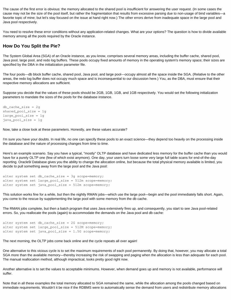
The cause of the first error is obvious: the memory allocated to the shared pool is insufficient for answering the user request. (In some cases the cause may not be the size of the pool itself, but rather the fragmentation that results from excessive parsing due to non-usage of bind variables—a favorite topic of mine; but let's stay focused on the issue at hand right now.) The other errors derive from inadequate space in the large pool and Java pool respectively.

You need to resolve these error conditions without any application-related changes. What are your options? The question is how to divide available memory among all the pools required by the Oracle instance.

How Do You Split the Pie?

The System Global Area (SGA) of an Oracle instance, as you know, comprises several memory areas, including the buffer cache, shared pool, Java pool, large pool, and redo log buffers. These pools occupy fixed amounts of memory in the operating system's memory space; their sizes are specified by the DBA in the initialization parameter file.

The four pools—db block buffer cache, shared pool, Java pool, and large pool—occupy almost all the space inside the SGA. (Relative to the other areas, the redo log buffer does not occupy much space and is inconsequential to our discussion here.) You, as the DBA, must ensure that their respective memory allocations are sufficient.

Suppose you decide that the values of these pools should be 2GB, 1GB, 1GB, and 1GB respectively. You would set the following initialization parameters to mandate the sizes of the pools for the database instance.

db_cache_size = 2gshared_pool_size = 1glarge_pool_size = 1gjava_pool_size = 1g

Now, take a close look at these parameters. Honestly, are these values accurate?

I'm sure you have your doubts. In real life, no one can specify these pools to an exact science—they depend too heavily on the processing inside the database and the nature of processing changes from time to time.

Here's an example scenario. Say you have a typical, "mostly" OLTP database and have dedicated less memory for the buffer cache than you would have for a purely OLTP one (few of which exist anymore). One day, your users turn loose some very large full table scans for end-of-the-day reporting. Oracle9i Database gives you the ability to change the allocation online, but because the total physical memory available is limited, you decide to pull something away from the large pool and the Java pool:

alter system set db_cache_size = 3g scope=memory;alter system set large_pool_size = 512m scope=memory;alter system set java_pool_size = 512m scope=memory;

This solution works fine for a while, but then the nightly RMAN jobs—which use the large pool—begin and the pool immediately falls short. Again, you come to the rescue by supplementing the large pool with some memory from the db cache.

The RMAN jobs complete, but then a batch program that uses Java extensively fires up, and consequently, you start to see Java pool-related errors. So, you reallocate the pools (again) to accommodate the demands on the Java pool and db cache:

alter system set db_cache_size = 2G scope=memory;alter system set large_pool_size = 512M scope=memory;alter system set java_pool_size = 1.5G scope=memory;

The next morning, the OLTP jobs come back online and the cycle repeats all over again!

One alternative to this vicious cycle is to set the maximum requirements of each pool permanently. By doing that, however, you may allocate a total SGA more than the available memory—thereby increasing the risk of swapping and paging when the allocation is less than adequate for each pool. The manual reallocation method, although impractical, looks pretty good right now.

Another alternative is to set the values to acceptable minimums. However, when demand goes up and memory is not available, performance will suffer.

Note that in all these examples the total memory allocated to SGA remained the same, while the allocation among the pools changed based on immediate requirements. Wouldn't it be nice if the RDBMS were to automatically sense the demand from users and redistribute memory allocations

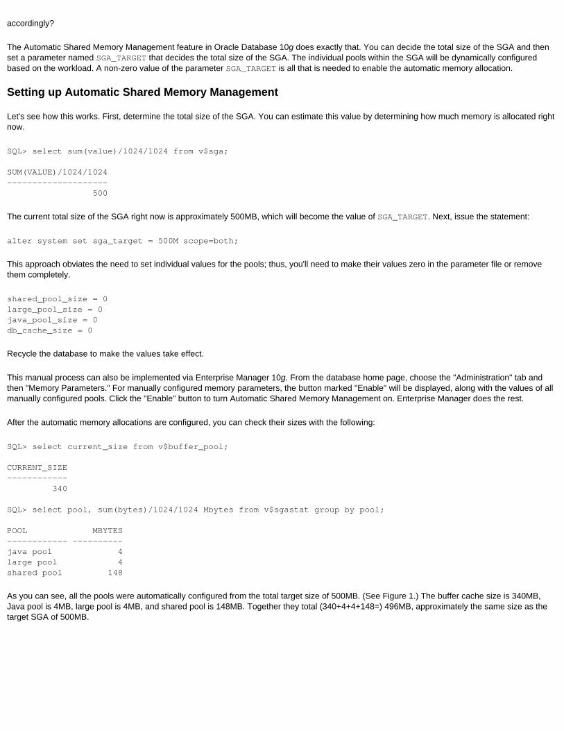
accordingly?

The Automatic Shared Memory Management feature in Oracle Database 10g does exactly that. You can decide the total size of the SGA and then set a parameter named SGA_TARGET that decides the total size of the SGA. The individual pools within the SGA will be dynamically configured based on the workload. A non-zero value of the parameter SGA_TARGET is all that is needed to enable the automatic memory allocation.

Setting up Automatic Shared Memory Management

Let's see how this works. First, determine the total size of the SGA. You can estimate this value by determining how much memory is allocated right now.

SQL> select sum(value)/1024/1024 from v$sga;

SUM(VALUE)/1024/1024-------------------- 500

The current total size of the SGA right now is approximately 500MB, which will become the value of SGA_TARGET. Next, issue the statement:

alter system set sga_target = 500M scope=both;

This approach obviates the need to set individual values for the pools; thus, you'll need to make their values zero in the parameter file or remove them completely.

shared_pool_size = 0large_pool_size = 0java_pool_size = 0db_cache_size = 0

Recycle the database to make the values take effect.

This manual process can also be implemented via Enterprise Manager 10g. From the database home page, choose the "Administration" tab and then "Memory Parameters." For manually configured memory parameters, the button marked "Enable" will be displayed, along with the values of all manually configured pools. Click the "Enable" button to turn Automatic Shared Memory Management on. Enterprise Manager does the rest.

After the automatic memory allocations are configured, you can check their sizes with the following:

SQL> select current_size from v$buffer_pool;

CURRENT_SIZE------------ 340

SQL> select pool, sum(bytes)/1024/1024 Mbytes from v$sgastat group by pool;

POOL MBYTES------------ ----------java pool 4large pool 4shared pool 148

As you can see, all the pools were automatically configured from the total target size of 500MB. (See Figure 1.) The buffer cache size is 340MB, Java pool is 4MB, large pool is 4MB, and shared pool is 148MB. Together they total (340+4+4+148=) 496MB, approximately the same size as the target SGA of 500MB.

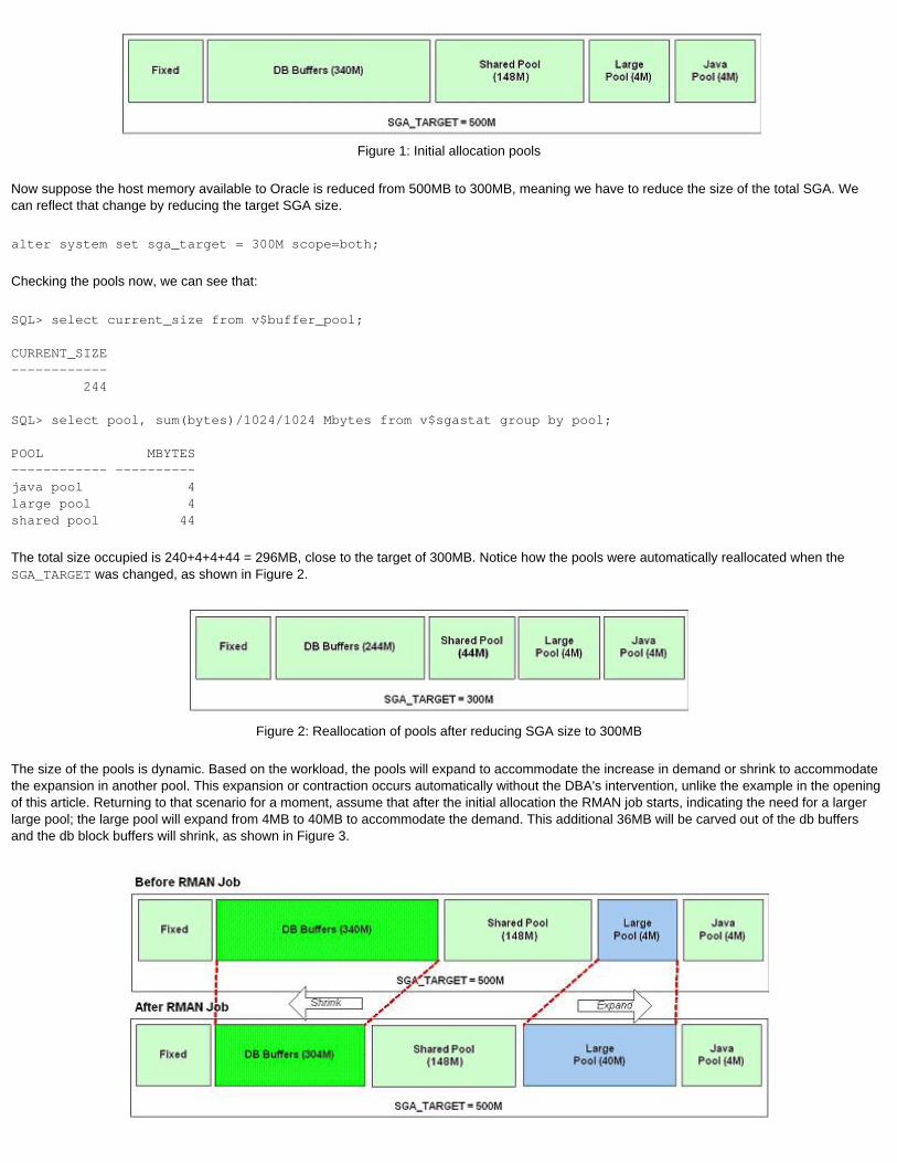
Figure 1: Initial allocation pools

Now suppose the host memory available to Oracle is reduced from 500MB to 300MB, meaning we have to reduce the size of the total SGA. We can reflect that change by reducing the target SGA size.

alter system set sga_target = 300M scope=both;

Checking the pools now, we can see that:

SQL> select current_size from v$buffer_pool;

CURRENT_SIZE------------ 244

SQL> select pool, sum(bytes)/1024/1024 Mbytes from v$sgastat group by pool;

POOL MBYTES------------ ----------java pool 4large pool 4shared pool 44

The total size occupied is 240+4+4+44 = 296MB, close to the target of 300MB. Notice how the pools were automatically reallocated when the SGA_TARGET was changed, as shown in Figure 2.

Figure 2: Reallocation of pools after reducing SGA size to 300MB

The size of the pools is dynamic. Based on the workload, the pools will expand to accommodate the increase in demand or shrink to accommodate the expansion in another pool. This expansion or contraction occurs automatically without the DBA's intervention, unlike the example in the opening of this article. Returning to that scenario for a moment, assume that after the initial allocation the RMAN job starts, indicating the need for a larger large pool; the large pool will expand from 4MB to 40MB to accommodate the demand. This additional 36MB will be carved out of the db buffers and the db block buffers will shrink, as shown in Figure 3.

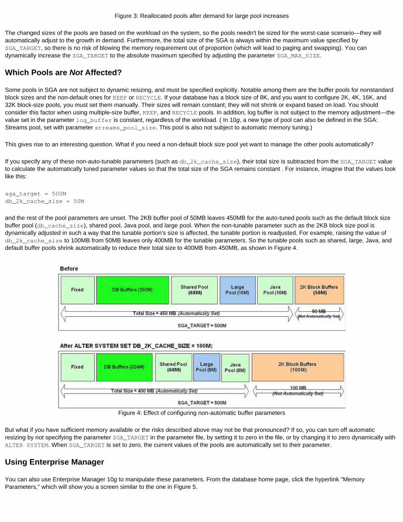
Figure 3: Reallocated pools after demand for large pool increases

The changed sizes of the pools are based on the workload on the system, so the pools needn't be sized for the worst-case scenario—they will automatically adjust to the growth in demand. Furthermore, the total size of the SGA is always within the maximum value specified by SGA_TARGET, so there is no risk of blowing the memory requirement out of proportion (which will lead to paging and swapping). You can dynamically increase the SGA_TARGET to the absolute maximum specified by adjusting the parameter SGA_MAX_SIZE.

Which Pools are Not Affected?

Some pools in SGA are not subject to dynamic resizing, and must be specified explicitly. Notable among them are the buffer pools for nonstandard block sizes and the non-default ones for KEEP or RECYCLE. If your database has a block size of 8K, and you want to configure 2K, 4K, 16K, and 32K block-size pools, you must set them manually. Their sizes will remain constant; they will not shrink or expand based on load. You should consider this factor when using multiple-size buffer, KEEP, and RECYCLE pools. In addition, log buffer is not subject to the memory adjustment—the value set in the parameter log_buffer is constant, regardless of the workload. ( In 10g, a new type of pool can also be defined in the SGA: Streams pool, set with parameter streams_pool_size. This pool is also not subject to automatic memory tuning.)

This gives rise to an interesting question. What if you need a non-default block size pool yet want to manage the other pools automatically?

If you specify any of these non-auto-tunable parameters (such as db_2k_cache_size), their total size is subtracted from the SGA_TARGET value to calculate the automatically tuned parameter values so that the total size of the SGA remains constant . For instance, imagine that the values look like this:

sga_target = 500Mdb_2k_cache_size = 50M

and the rest of the pool parameters are unset. The 2KB buffer pool of 50MB leaves 450MB for the auto-tuned pools such as the default block size buffer pool (db_cache_size), shared pool, Java pool, and large pool. When the non-tunable parameter such as the 2KB block size pool is dynamically adjusted in such a way that the tunable portion's size is affected, the tunable portion is readjusted. For example, raising the value of db_2k_cache_size to 100MB from 50MB leaves only 400MB for the tunable parameters. So the tunable pools such as shared, large, Java, and default buffer pools shrink automatically to reduce their total size to 400MB from 450MB, as shown in Figure 4.

Figure 4: Effect of configuring non-automatic buffer parameters

But what if you have sufficient memory available or the risks described above may not be that pronounced? If so, you can turn off automatic resizing by not specifying the parameter SGA_TARGET in the parameter file, by setting it to zero in the file, or by changing it to zero dynamically with ALTER SYSTEM. When SGA_TARGET is set to zero, the current values of the pools are automatically set to their parameter.

Using Enterprise Manager

You can also use Enterprise Manager 10g to manipulate these parameters. From the database home page, click the hyperlink "Memory Parameters," which will show you a screen similar to the one in Figure 5.

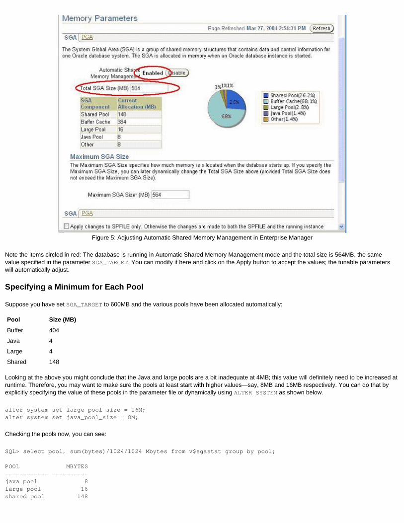
Figure 5: Adjusting Automatic Shared Memory Management in Enterprise Manager

Note the items circled in red: The database is running in Automatic Shared Memory Management mode and the total size is 564MB, the same value specified in the parameter SGA_TARGET. You can modify it here and click on the Apply button to accept the values; the tunable parameters will automatically adjust.

Specifying a Minimum for Each Pool

Suppose you have set SGA_TARGET to 600MB and the various pools have been allocated automatically:

Pool Size (MB)

Buffer 404

Java 4

Large 4

Shared 148

Looking at the above you might conclude that the Java and large pools are a bit inadequate at 4MB; this value will definitely need to be increased at runtime. Therefore, you may want to make sure the pools at least start with higher values—say, 8MB and 16MB respectively. You can do that by explicitly specifying the value of these pools in the parameter file or dynamically using ALTER SYSTEM as shown below.

alter system set large_pool_size = 16M;alter system set java_pool_size = 8M;

Checking the pools now, you can see:

SQL> select pool, sum(bytes)/1024/1024 Mbytes from v$sgastat group by pool;

POOL MBYTES------------ ----------java pool 8large pool 16shared pool 148

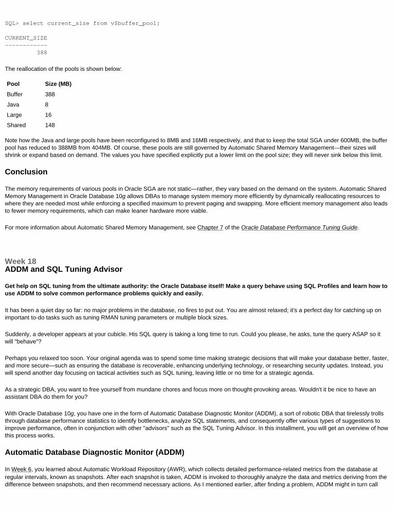
SQL> select current_size from v$buffer_pool;

CURRENT_SIZE------------ 388

The reallocation of the pools is shown below:

Pool Size (MB)

Buffer 388

Java 8

Large 16

Shared 148

Note how the Java and large pools have been reconfigured to 8MB and 16MB respectively, and that to keep the total SGA under 600MB, the buffer pool has reduced to 388MB from 404MB. Of course, these pools are still governed by Automatic Shared Memory Management—their sizes will shrink or expand based on demand. The values you have specified explicitly put a lower limit on the pool size; they will never sink below this limit.

Conclusion

The memory requirements of various pools in Oracle SGA are not static—rather, they vary based on the demand on the system. Automatic Shared Memory Management in Oracle Database 10g allows DBAs to manage system memory more efficiently by dynamically reallocating resources to where they are needed most while enforcing a specified maximum to prevent paging and swapping. More efficient memory management also leads to fewer memory requirements, which can make leaner hardware more viable.

For more information about Automatic Shared Memory Management, see Chapter 7 of the Oracle Database Performance Tuning Guide.

Week 18ADDM and SQL Tuning Advisor

Get help on SQL tuning from the ultimate authority: the Oracle Database itself! Make a query behave using SQL Profiles and learn how to use ADDM to solve common performance problems quickly and easily.

It has been a quiet day so far: no major problems in the database, no fires to put out. You are almost relaxed; it's a perfect day for catching up on important to-do tasks such as tuning RMAN tuning parameters or multiple block sizes.

Suddenly, a developer appears at your cubicle. His SQL query is taking a long time to run. Could you please, he asks, tune the query ASAP so it will "behave"?

Perhaps you relaxed too soon. Your original agenda was to spend some time making strategic decisions that will make your database better, faster, and more secure—such as ensuring the database is recoverable, enhancing underlying technology, or researching security updates. Instead, you will spend another day focusing on tactical activities such as SQL tuning, leaving little or no time for a strategic agenda.

As a strategic DBA, you want to free yourself from mundane chores and focus more on thought-provoking areas. Wouldn't it be nice to have an assistant DBA do them for you?

With Oracle Database 10g, you have one in the form of Automatic Database Diagnostic Monitor (ADDM), a sort of robotic DBA that tirelessly trolls through database performance statistics to identify bottlenecks, analyze SQL statements, and consequently offer various types of suggestions to improve performance, often in conjunction with other "advisors" such as the SQL Tuning Advisor. In this installment, you will get an overview of how this process works.

Automatic Database Diagnostic Monitor (ADDM)

In Week 6, you learned about Automatic Workload Repository (AWR), which collects detailed performance-related metrics from the database at regular intervals, known as snapshots. After each snapshot is taken, ADDM is invoked to thoroughly analyze the data and metrics deriving from the difference between snapshots, and then recommend necessary actions. As I mentioned earlier, after finding a problem, ADDM might in turn call

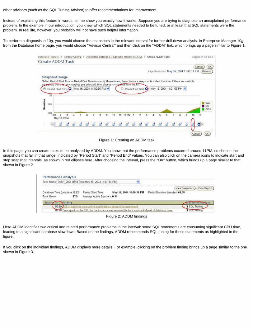
other advisors (such as the SQL Tuning Advisor) to offer recommendations for improvement.

Instead of explaining this feature in words, let me show you exactly how it works. Suppose you are trying to diagnose an unexplained performance problem. In the example in our introduction, you knew which SQL statements needed to be tuned, or at least that SQL statements were the problem. In real life, however, you probably will not have such helpful information.

To perform a diagnosis in 10g, you would choose the snapshots in the relevant interval for further drill-down analysis. In Enterprise Manager 10g, from the Database home page, you would choose "Advisor Central" and then click on the "ADDM" link, which brings up a page similar to Figure 1.

Figure 1: Creating an ADDM task

In this page, you can create tasks to be analyzed by ADDM. You know that the performance problems occurred around 11PM, so choose the snapshots that fall in that range, indicated by "Period Start" and "Period End" values. You can also click on the camera icons to indicate start and stop snapshot intervals, as shown in red ellipses here. After choosing the interval, press the "OK" button, which brings up a page similar to that shown in Figure 2.

Figure 2: ADDM findings

Here ADDM identifies two critical and related performance problems in the interval: some SQL statements are consuming significant CPU time, leading to a significant database slowdown. Based on the findings, ADDM recommends SQL tuning for these statements as highlighted in the figure.

If you click on the individual findings, ADDM displays more details. For example, clicking on the problem finding brings up a page similar to the one shown in Figure 3.

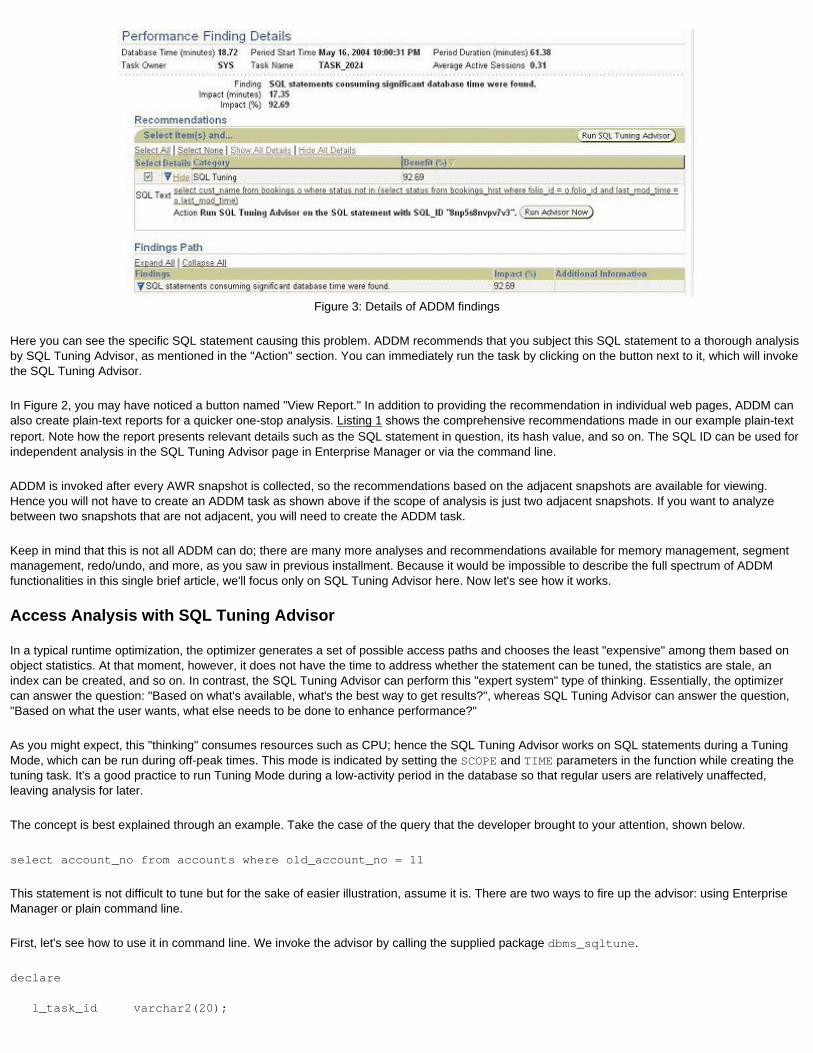
Figure 3: Details of ADDM findings

Here you can see the specific SQL statement causing this problem. ADDM recommends that you subject this SQL statement to a thorough analysis by SQL Tuning Advisor, as mentioned in the "Action" section. You can immediately run the task by clicking on the button next to it, which will invoke the SQL Tuning Advisor.

In Figure 2, you may have noticed a button named "View Report." In addition to providing the recommendation in individual web pages, ADDM can also create plain-text reports for a quicker one-stop analysis. Listing 1 shows the comprehensive recommendations made in our example plain-text report. Note how the report presents relevant details such as the SQL statement in question, its hash value, and so on. The SQL ID can be used for independent analysis in the SQL Tuning Advisor page in Enterprise Manager or via the command line.

ADDM is invoked after every AWR snapshot is collected, so the recommendations based on the adjacent snapshots are available for viewing. Hence you will not have to create an ADDM task as shown above if the scope of analysis is just two adjacent snapshots. If you want to analyze between two snapshots that are not adjacent, you will need to create the ADDM task.

Keep in mind that this is not all ADDM can do; there are many more analyses and recommendations available for memory management, segment management, redo/undo, and more, as you saw in previous installment. Because it would be impossible to describe the full spectrum of ADDM functionalities in this single brief article, we'll focus only on SQL Tuning Advisor here. Now let's see how it works.

Access Analysis with SQL Tuning Advisor

In a typical runtime optimization, the optimizer generates a set of possible access paths and chooses the least "expensive" among them based on object statistics. At that moment, however, it does not have the time to address whether the statement can be tuned, the statistics are stale, an index can be created, and so on. In contrast, the SQL Tuning Advisor can perform this "expert system" type of thinking. Essentially, the optimizer can answer the question: "Based on what's available, what's the best way to get results?", whereas SQL Tuning Advisor can answer the question, "Based on what the user wants, what else needs to be done to enhance performance?"

As you might expect, this "thinking" consumes resources such as CPU; hence the SQL Tuning Advisor works on SQL statements during a Tuning Mode, which can be run during off-peak times. This mode is indicated by setting the SCOPE and TIME parameters in the function while creating the tuning task. It's a good practice to run Tuning Mode during a low-activity period in the database so that regular users are relatively unaffected, leaving analysis for later.

The concept is best explained through an example. Take the case of the query that the developer brought to your attention, shown below.

select account_no from accounts where old_account_no = 11

This statement is not difficult to tune but for the sake of easier illustration, assume it is. There are two ways to fire up the advisor: using Enterprise Manager or plain command line.

First, let's see how to use it in command line. We invoke the advisor by calling the supplied package dbms_sqltune.

declare

l_task_id varchar2(20);

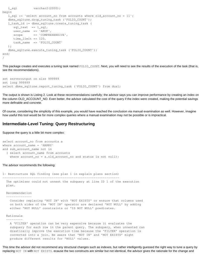
l_sql varchar2(2000);begin l_sql := 'select account_no from accounts where old_account_no = 11'; dbms_sqltune.drop_tuning_task ('FOLIO_COUNT'); l_task_id := dbms_sqltune.create_tuning_task ( sql_text => l_sql, user_name => 'ARUP', scope => 'COMPREHENSIVE', time_limit => 120, task_name => 'FOLIO_COUNT' ); dbms_sqltune.execute_tuning_task ('FOLIO_COUNT');end;/

This package creates and executes a tuning task named FOLIO_COUNT. Next, you will need to see the results of the execution of the task (that is, see the recommendations).

set serveroutput on size 999999set long 999999select dbms_sqltune.report_tuning_task ('FOLIO_COUNT') from dual;

The output is shown is Listing 2. Look at these recommendations carefully; the advisor says you can improve performance by creating an index on the column OLD_ACCOUNT_NO. Even better, the advisor calculated the cost of the query if the index were created, making the potential savings more definable and concrete.

Of course, considering the simplicity of this example, you would have reached the conclusion via manual examination as well. However, imagine how useful this tool would be for more complex queries where a manual examination may not be possible or is impractical.

Intermediate-Level Tuning: Query Restructuring

Suppose the query is a little bit more complex:

select account_no from accounts a where account_name = 'HARRY' and sub_account_name not in ( select account_name from accounts where account_no = a.old_account_no and status is not null);

The advisor recommends the following:

1- Restructure SQL finding (see plan 1 in explain plans section)---------------------------------------------------------------- The optimizer could not unnest the subquery at line ID 1 of the execution plan.

Recommendation -------------- Consider replacing "NOT IN" with "NOT EXISTS" or ensure that columns used on both sides of the "NOT IN" operator are declared "NOT NULL" by adding either "NOT NULL" constraints or "IS NOT NULL" predicates.

Rationale --------- A "FILTER" operation can be very expensive because it evaluates the subquery for each row in the parent query. The subquery, when unnested can drastically improve the execution time because the "FILTER" operation is converted into a join. Be aware that "NOT IN" and "NOT EXISTS" might produce different results for "NULL" values.

This time the advisor did not recommend any structural changes such as indexes, but rather intelligently guessed the right way to tune a query by replacing NOT IN with NOT EXISTS. ecause the two constructs are similar but not identical, the advisor gives the rationale for the change and

leaves the decision to the DBA or application developer to decide whether this recommendation is valid for the environment.

Advanced Tuning: SQL Profiles

As you may know, the optimizer decides on a query execution plan by examining the statistics present on the objects referenced in the query and then calculating the least-cost method. If a query involves more than one table, which is typical, the optimizer calculates the least-cost option by examining the statistics of all the referenced objects—but it does not know the relationship among them.

For example, assume that an account with status DELINQUENT will have less than $1,000 as balance. A query that joins the tables ACCOUNTS and BALANCES will report fewer rows if the predicate has a clause filtering for DELINQUENT only. The optimizer does not know this complex relationship—but the advisor does; it "assembles" this relationship from the data and stores it in the form of a SQL Profile. With access to the SQL Profile, the optimizer not only knows the data distribution of tables, but also the data correlations among them. This additional information allows the optimizer to generate a superior execution plan, thereby resulting in a well-tuned query.

SQL Profiles obviate the need for tuning SQL statements by manually adding query hints to the code. Consequently, the SQL Tuning Advisor makes it possible to tune packaged applications without modifying code—a tremendous benefit.

The main point here is that unlike objects statistics, a SQL Profile is mapped to a query, not an object or objects. Another query involving the same two tables—ACCOUNTS and BALANCES—may have a different profile. Using this metadata information on the query, Oracle can improve performance.

If a profile can be created, it is done during the SQL Tuning Advisor session, where the advisor generates the profile and recommends that you "Accept" it. Unless a profile is accepted, it's not tied to a statement. You can accept the profile at any time by issuing a statement such as the following:

begin dbms_sqltune.accept_sql_profile ( task_name => 'FOLIO_COUNT', name => 'FOLIO_COUNT_PROFILE' description => 'Folio Count Profile', category => 'FOLIO_COUNT');end;

This command ties the profile named FOLIO_COUNT_PROFILE generated earlier by the advisor to the statement associated with the tuning task named FOLIO_COUNT described in the earlier example. (Note that although only the advisor, not the DBA, can create a SQL Profile, only you can decide when to use it.)

You can see created SQL Profiles in the dictionary view DBA_SQL_PROFILES. The column SQL_TEXT shows the SQL statement the profile was assigned to; the column STATUS indicates if the profile is enabled. (Even if it is already tied to a statement, the profile must be enabled in order to affect the execution plan.)

Using ADDM and SQL Tuning Advisor

In addition to the three cases described above, SQL Tuning Advisor also identifies any objects with missing statistics referenced in the query. Thus, the advisor performs four distinct types of tasks:

● Checks if objects have valid, usable statistics for proper optimization● Attempts to rewrite queries for better performance and suggests rewriting● Checks the access path to see if performance could be improved by adding additional structures such as indexes and materialized views● Creates SQL profiles and attaches them to specific queries.

Based on these capabilities, I can think of at least three different scenarios in which ADDM and SQL Tuning Advisor serve as powerful tools:

● Reactive Tuning: Your application suddenly starts to perform poorly. Using ADDM, you can drill the problem down to a SQL statement or a set of statements, as shown in the section on ADDM. Following the recommendation of ADDM, you can launch SQL Tuning Advisor and correct the problem.

● Proactive Tuning: The application behaves acceptably well; however, you want to make sure that all necessary maintenance tasks are performed and know if queries can be tuned even more. You would fire up SQL Tuning Advisor in the standalone mode to identify possible tuning alternatives.

● Development Tuning: While code is being tested in development there are many opportunities to tune the query, as opposed to wthe QA or production phases. You can use the command-line version of the advisor to tune individual SQL statements before they are finalized in

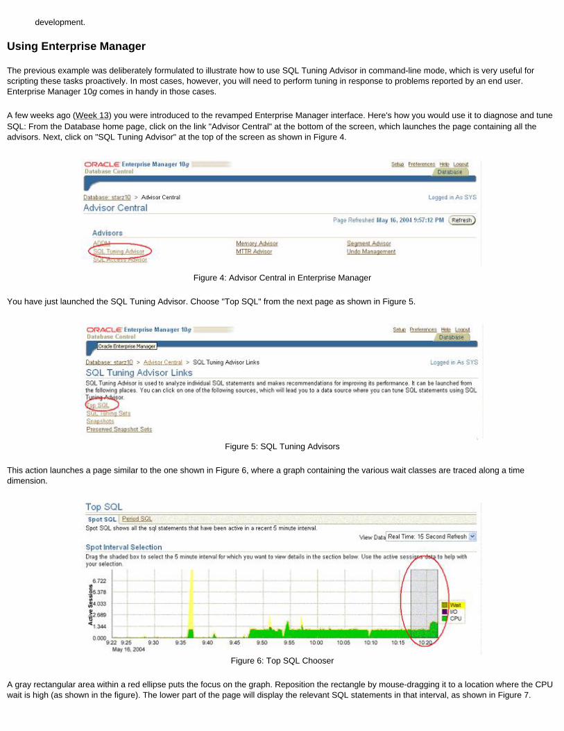
development.

Using Enterprise Manager

The previous example was deliberately formulated to illustrate how to use SQL Tuning Advisor in command-line mode, which is very useful for scripting these tasks proactively. In most cases, however, you will need to perform tuning in response to problems reported by an end user. Enterprise Manager 10g comes in handy in those cases.

A few weeks ago (Week 13) you were introduced to the revamped Enterprise Manager interface. Here's how you would use it to diagnose and tune SQL: From the Database home page, click on the link "Advisor Central" at the bottom of the screen, which launches the page containing all the advisors. Next, click on "SQL Tuning Advisor" at the top of the screen as shown in Figure 4.

Figure 4: Advisor Central in Enterprise Manager

You have just launched the SQL Tuning Advisor. Choose "Top SQL" from the next page as shown in Figure 5.

Figure 5: SQL Tuning Advisors

This action launches a page similar to the one shown in Figure 6, where a graph containing the various wait classes are traced along a time dimension.

Figure 6: Top SQL Chooser

A gray rectangular area within a red ellipse puts the focus on the graph. Reposition the rectangle by mouse-dragging it to a location where the CPU wait is high (as shown in the figure). The lower part of the page will display the relevant SQL statements in that interval, as shown in Figure 7.

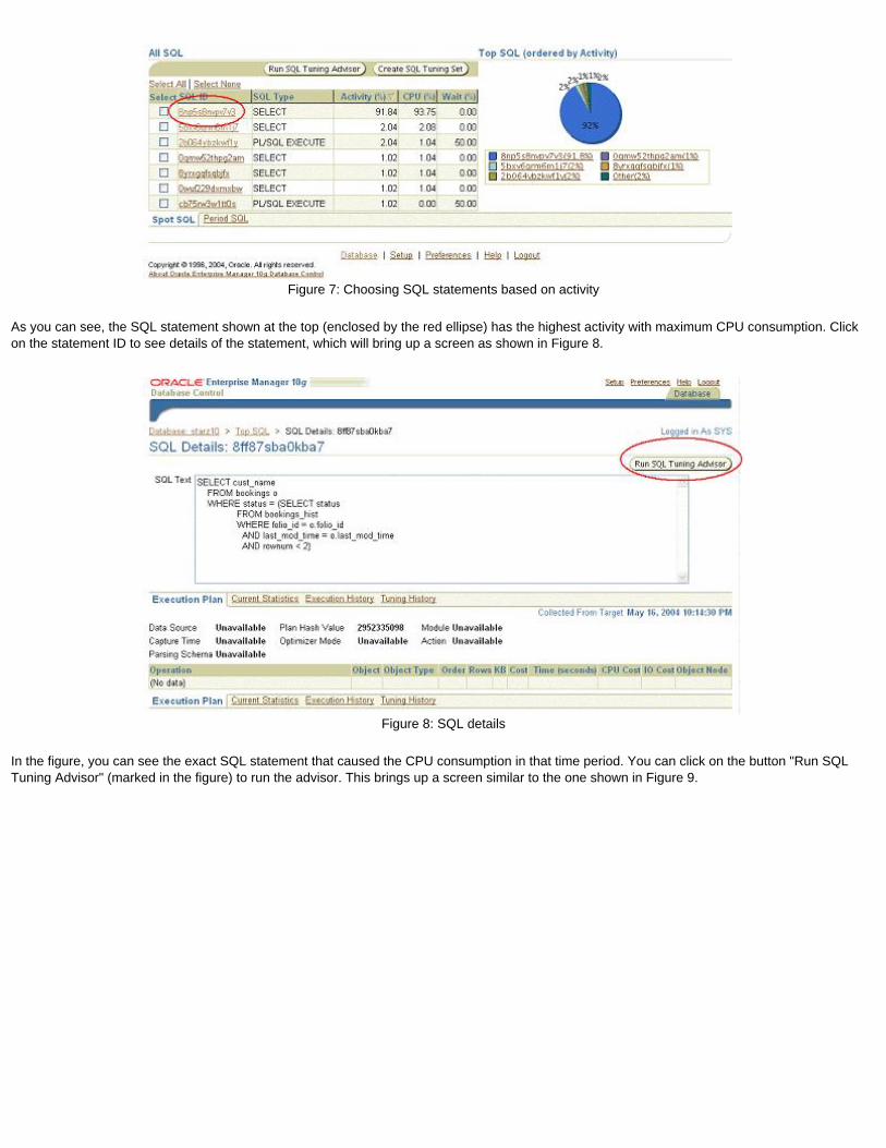
Figure 7: Choosing SQL statements based on activity

As you can see, the SQL statement shown at the top (enclosed by the red ellipse) has the highest activity with maximum CPU consumption. Click on the statement ID to see details of the statement, which will bring up a screen as shown in Figure 8.

Figure 8: SQL details

In the figure, you can see the exact SQL statement that caused the CPU consumption in that time period. You can click on the button "Run SQL Tuning Advisor" (marked in the figure) to run the advisor. This brings up a screen similar to the one shown in Figure 9.

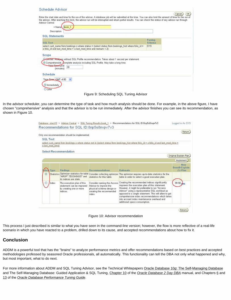
Figure 9: Scheduling SQL Tuning Advisor

In the advisor scheduler, you can determine the type of task and how much analysis should be done. For example, in the above figure, I have chosen "comprehensive" analysis and that the advisor is to be run immediately. After the advisor finishes you can see its recommendation, as shown in Figure 10.

Figure 10: Advisor recommendation

This process I just described is similar to what you have seen in the command-line version; however, the flow is more reflective of a real-life scenario in which you have reacted to a problem, drilled down to its cause, and accepted recommendations about how to fix it.

Conclusion

ADDM is a powerful tool that has the "brains" to analyze performance metrics and offer recommendations based on best practices and accepted methodologies professed by seasoned Oracle professionals, all automatically. This functionality can tell the DBA not only what happened and why, but most important, what to do next.

For more information about ADDM and SQL Tuning Advisor, see the Technical Whitepapers Oracle Database 10g: The Self-Managing Database and The Self-Managing Database: Guided Application & SQL Tuning, Chapter 10 of the Oracle Database 2 Day DBA manual, and Chapters 6 and 13 of the Oracle Database Performance Tuning Guide.

Week 19Scheduler

Tired of cumbersome manual management of intervals in dbms_job and need a new scheduling system inside the database? Look no further than the database itself.

Some of you may use the dbms_job package extensively to submit database jobs to be run in the background, control the time or interval of a run, report failures, and much more. However, I have a feeling that most of you don't.

The problem with the package is that it can handle only PL/SQL code segments—just anonymous blocks and stored program units. It cannot handle anything outside the database that is in an operating system command file or executable. To do so, you would have to resort to using an operating system scheduling utility such as cron in Unix or the AT command in Windows. Or, you could use a third-party tool, one that may even extend this functionality by providing a graphical user interface.

Even so, dbms_job has a distinct advantage over these alternatives: it is active only when the database is up and running. If the database is down, the jobs don't run. A tool outside the database must manually check if the database is up—and that can be difficult. Another advantage is that dbms_job is internal to the database; hence you can access it via a database access utility such as SQL*Plus.

The Oracle Database 10g Scheduler feature offers the best of all worlds: a job scheduler utility right inside the database that is sufficiently powerful to handle all types of jobs, not just PL/SQL code segments, and that can help you create jobs either with or without associated programs and/or schedules. Best of all, it comes with the database at no additional cost. In this installment, we'll take a look at how it works.

Creating Jobs Without Programs

Perhaps the concept can be best introduced through examples. Suppose you have created a shell script to move archived log files to a different filesystem as follows:

/home/arup/dbtools/move_arcs.sh

We can specify the OS executable directly without creating it as a program first.

begin dbms_scheduler.create_job ( job_name => 'ARC_MOVE_2', schedule_name => 'EVERY_30_MINS', job_type => 'EXECUTABLE', job_action => '/home/arup/dbtools/move_arcs.sh', enabled => true, comments => 'Move Archived Logs to a Different Directory' );end;/

Similarly, you can create a job without a named schedule.

begin dbms_scheduler.create_job ( job_name => 'ARC_MOVE_3', job_type => 'EXECUTABLE', job_action => '/home/arup/dbtools/move_arcs.sh', repeat_interval => 'FREQ=MINUTELY; INTERVAL=30', enabled => true, comments => 'Move Archived Logs to a Different Directory' );end;/

One advantage of Scheduler over dbms_job is pretty clear from our initial example: the ability to call OS utilities and programs, not just PL/SQL

program units. This ability makes it the most comprehensive job management tool for managing Oracle Database and related jobs. However, you may have noted another, equally important advantage: the ability to define intervals in natural language. Note that in the above example we wanted our schedule to run every 30 minutes; hence the parameter REPEAT_INTERVAL is defined with a simple, English-like expression (not a PL/SQL one) :

'FREQ=MINUTELY; INTERVAL=30'

A more complex example may help convey this advantage even better. Suppose your production applications become most active at 7:00AM and 3:00PM. To collect system statistics, you want to run Statspack from Monday to Friday at 7:00AM and 3:00PM only. If you use DBMS_JOB.SUBMIT to create a job, the NEXT_DATE parameter will look something like this:

DECODE( SIGN ( 15 - TO_CHAR(SYSDATE,'HH24') ), 1, TRUNC(SYSDATE)+15/24, TRUNC ( SYSDATE + DECODE ( TO_CHAR(SYSDATE,'D'), 6, 3, 1 ) ) +7/24)

Is that code easy to understand? Not really.

Now let's see the equivalent job in DBMS_SCHEDULER. The parameter REPEAT_INTERVAL will be as simple as:

'FREQ=DAILY; BYDAY=MON,TUE,WED,THU,FRI; BYHOUR=7,15'

Furthermore, this parameter value can accept a variety of intervals, some of them very powerful. Here are some more examples:

● Last Sunday of every month:

FREQ=MONTHLY; BYDAY=-1SUN

● Every third Friday of the month:

FREQ=MONTHLY; BYDAY=3FRI

● Every second Friday from the end of the month, not from the beginning:

FREQ=MONTHLY; BYDAY=-2FRI

The minus signs before the numbers indicate counting from the end, instead of the beginning.

What if you wanted to verify if the interval settings are correct? Wouldn't it be nice to see the various dates constructed from the calendar string? Well, you can get a preview of the calculation of next dates using the EVALUATE_CALENDAR_STRING procedure. Using the first example—running Statspack every day from Monday through Friday at 7:00AM and 3:00PM—you can check the accuracy of your interval string as follows:

set serveroutput on size 999999

declare L_start_date TIMESTAMP; l_next_date TIMESTAMP;

l_return_date TIMESTAMP;begin l_start_date := trunc(SYSTIMESTAMP); l_return_date := l_start_date; for ctr in 1..10 loop dbms_scheduler.evaluate_calendar_string( 'FREQ=DAILY; BYDAY=MON,TUE,WED,THU,FRI; BYHOUR=7,15', l_start_date, l_return_date, l_next_date ); dbms_output.put_line('Next Run on: ' || to_char(l_next_date,'mm/dd/yyyy hh24:mi:ss') ); l_return_date := l_next_date; end loop;end;/

The output is:

Next Run on: 03/22/2004 07:00:00Next Run on: 03/22/2004 15:00:00Next Run on: 03/23/2004 07:00:00Next Run on: 03/23/2004 15:00:00Next Run on: 03/24/2004 07:00:00Next Run on: 03/24/2004 15:00:00Next Run on: 03/25/2004 07:00:00Next Run on: 03/25/2004 15:00:00Next Run on: 03/26/2004 07:00:00Next Run on: 03/26/2004 15:00:00

This confirms that your settings are correct.

Associating Jobs with Programs

In the above case, you created a job independently of any program. Now let's create one that refers to an operating system utility or program, a schedule to specify how many times something should run, and then join the two to create a job.

First you need to make the database aware that your script is a program to be used in a job. To create this program, you must have the CREATE JOB privilege.

begin dbms_scheduler.create_program ( program_name => 'MOVE_ARCS', program_type => 'EXECUTABLE', program_action => '/home/arup/dbtools/move_arcs.sh', enabled => TRUE, comments => 'Moving Archived Logs to Staging Directory' );end;/

Here you have created a named program unit, specified it as an executable, and noted what the program unit is called.

Next, you will create a named schedule to be run every 30 minutes called EVERY_30_MINS. You would do that with:

begin dbms_scheduler.create_schedule ( schedule_name => 'EVERY_30_MINS', repeat_interval => 'FREQ=MINUTELY; INTERVAL=30', comments => 'Every 30-mins'

);end;/

Now that the program and schedule are created, you will associate the program to the schedule to create a job.

begin dbms_scheduler.create_job ( job_name => 'ARC_MOVE', program_name => 'MOVE_ARCS', schedule_name => 'EVERY_30_MINS', comments => 'Move Archived Logs to a Different Directory', enabled => TRUE );end;/

This will create a job to be run every 30 minutes that executes the shell script move_arcs.sh. It will be handled by the Scheduler feature inside the database—no need for cron or the AT utility.

Classes, Plans, and Windows

A good job scheduling system worth its salt must support the ability to prioritize jobs. For instance, the statistics collection job suddenly goes into the OLTP workload window affecting performance there. To ensure the stats collection job doesn't consume resources affecting OLTP, you would use job classes, resource plans, and Scheduler Windows.

For example, while defining a job, you can make it part of a job class, which maps to a resource consumer group for allocation of resources. To do that, first you need to define a resource consumer group called, say, OLTP_GROUP.

begin dbms_resource_manager.clear_pending_area(); dbms_resource_manager.create_pending_area(); dbms_resource_manager.create_consumer_group ( consumer_group => 'oltp_group', comment => 'OLTP Activity Group' ); dbms_resource_manager.submit_pending_area();end;/

Next, you need to create a resource plan.

begin dbms_resource_manager.clear_pending_area(); dbms_resource_manager.create_pending_area(); dbms_resource_manager.create_plan ('OLTP_PLAN', 'OLTP Database Activity Plan'); dbms_resource_manager.create_plan_directive( plan => 'OLTP_PLAN', group_or_subplan => 'OLTP_GROUP', comment => 'This is the OLTP Plan', cpu_p1 => 80, cpu_p2 => NULL, cpu_p3 => NULL, cpu_p4 => NULL, cpu_p5 => NULL, cpu_p6 => NULL, cpu_p7 => NULL, cpu_p8 => NULL, parallel_degree_limit_p1 => 4, active_sess_pool_p1 => NULL, queueing_p1 => NULL, switch_group => 'OTHER_GROUPS', switch_time => 10, switch_estimate => true, max_est_exec_time => 10, undo_pool => 500, max_idle_time => NULL,

max_idle_blocker_time => NULL, switch_time_in_call => NULL ); dbms_resource_manager.create_plan_directive( plan => 'OLTP_PLAN', group_or_subplan => 'OTHER_GROUPS', comment => NULL, cpu_p1 => 20, cpu_p2 => NULL, cpu_p3 => NULL, cpu_p4 => NULL, cpu_p5 => NULL, cpu_p6 => NULL, cpu_p7 => NULL, cpu_p8 => NULL, parallel_degree_limit_p1 => 0, active_sess_pool_p1 => 0, queueing_p1 => 0, switch_group => NULL, switch_time => NULL, switch_estimate => false, max_est_exec_time => 0, undo_pool => 10, max_idle_time => NULL, max_idle_blocker_time => NULL, switch_time_in_call => NULL ); dbms_resource_manager.submit_pending_area();end;/

Finally, you create a job class with the resource consumer group created earlier.

begin dbms_scheduler.create_job_class( job_class_name => 'OLTP_JOBS', logging_level => DBMS_SCHEDULER.LOGGING_FULL, log_history => 45, resource_consumer_group => 'OLTP_GROUP', comments => 'OLTP Related Jobs' );end;/

Let's examine the various parameters in this call. The parameter LOGGING_LEVEL sets how much log data is tracked for the job class. The setting LOGGING_FULL indicates that all activities on jobs in this class—creation, deletion, run, alteration, and so on—will be recorded in the logs. The logs can be seen from the view DBA_SCHEDULER_JOB_LOG and are available for 45 days as specified in the parameter LOG_HISTORY (the default being 30 days). The resource consumer group associated with this class is also specified. The job classes can be seen from the view DBA_SCHEDULER_JOB_CLASSES.

When you create a job, you can optionally associate a class to it. For instance, while creating COLLECT_STATS, a job that collects optimizer statistics by executing a stored procedure collect_opt_stats(), you could have specified:

begin dbms_scheduler.create_job ( job_name => 'COLLECT_STATS', job_type => 'STORED_PROCEDURE', job_action => 'collect_opt_stats', job_class => 'OLTP_JOBS', repeat_interval => 'FREQ=WEEKLY; INTERVAL=1', enabled => true, comments => 'Collect Optimizer Stats' );end;/

This command will place the newly created job in the class OLTP_JOBS, which is then governed by the resource plan OLTP_GROUP, which will restrict how much CPU can be allocated to the process, the maximum number of executions before it is switched to a different group, the group to switch to, and so on. Any job defined in this class will be governed by the same resource plan directive. This capability is particularly useful for

preventing different types of jobs from taking over the resources of the system.

The Scheduler Window is a time frame with an associated resource plan used for activating that plan-thereby supporting different priorities for the jobs over a time frame. For example, some jobs, such as batch programs to update databases for real-time decision-support, need high priority during the day but become low priority at night (or vice-versa). You can implement this schedule by defining different resource plans and then activating them using Scheduler Windows.

Monitoring

After a job is issued, you can monitor its status from the view DBA_SCHEDULER_JOB_LOG, where the column STATUS shows the current status of the job. If it shows FAILED, you can drill down further to find out the cause from the view DBA_SCHEDULER_JOB_RUN_DETAILS.

Administration

So far, we've discussed how to create several types of objects: programs, schedules, job classes, and jobs. What if you want to modify some of them to adjust to changing needs? Well, you can do that via APIs provided in the DBMS_SCHEDULER package.

From the Database tab of the Enterprise Manager 10g home page, click on the Administration link. This will bring up the Administration Screen, shown in Figure 1. All the Scheduler related tasks are found under the heading "Scheduler" to the bottom right-hand corner, shown inside a red ellipse in the figure.

Figure 1: Administration page

All the tasks related to scheduler, such as creating, deleting, and maintaining jobs, can be easily accomplished through the hyper-linked task in this page. Let's see a few of these tasks. We created all these tasks earlier, so the clicking on the Jobs tab will show a screen similar to Figure 2.

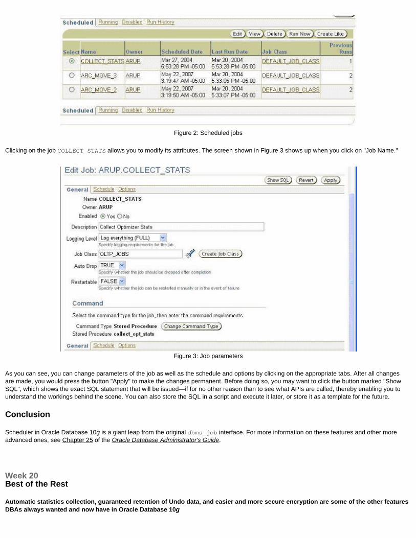
Figure 2: Scheduled jobs

Clicking on the job COLLECT_STATS allows you to modify its attributes. The screen shown in Figure 3 shows up when you click on "Job Name."

Figure 3: Job parameters

As you can see, you can change parameters of the job as well as the schedule and options by clicking on the appropriate tabs. After all changes are made, you would press the button "Apply" to make the changes permanent. Before doing so, you may want to click the button marked "Show SQL", which shows the exact SQL statement that will be issued—if for no other reason than to see what APIs are called, thereby enabling you to understand the workings behind the scene. You can also store the SQL in a script and execute it later, or store it as a template for the future.

Conclusion

Scheduler in Oracle Database 10g is a giant leap from the original dbms_job interface. For more information on these features and other more advanced ones, see Chapter 25 of the Oracle Database Administrator's Guide.

Week 20Best of the Rest

Automatic statistics collection, guaranteed retention of Undo data, and easier and more secure encryption are some of the other features DBAs always wanted and now have in Oracle Database 10g

Wow! This is the final week of our amazing journey into the most important new features for DBAs in Oracle Database 10g. Over these last 19 installments I have attempted to cover all the tools, tips, and techniques that have this fundamental appeal: making our jobs easier and more satisfying.

If a feature has "star" quality but still doesn't do much to help me as a DBA, it didn't make it on this list. Even so, 20 articles are not enough to explore all that Oracle 10g has to offer—I would probably need a hundred more. So in this penultimate installment of this series, I will describe just a few of the remaining new features of Oracle 10g that deserve to be mentioned.

Are Your Stats Stale? Don't Leave it to Chance

As most of you know, the Rules-Based Optimizer (RBO) is finally desupported (not deprecated) as of Oracle 10g. In anticipation of that long-awaited development, many Oracle9i Database shops upgraded to the Cost Based Optimizer (CBO) to get into the support loop and to take advantage of advanced features such as query rewrite and partition pruning. The problem, however, is statistics—or rather, the absence of them.

Because the CBO depends on accurate (or reasonably accurate) statistics to produce optimal execution paths, DBAs need to ensure that statistics are gathered regularly, creating yet another enforcement checklist. Prior to 10g, this process could be futile for various reasons. This difficulty gave rise to the theory that the CBO has a "mind of its own"—which implies behavior such as changing execution paths at will!

Many of these worries have been put to rest in 10g, in which statistics can be collected automatically. In Oracle9i, you could check if the data in a table had changed significantly by turning on the table monitoring option (ALTER TABLE ... MONITORING) and then checking the view DBA_TAB_MODIFICATIONS for those tables.

In 10g, the MONITORING statement is gone. Instead, statistics are collected automatically if the initialization parameter STATISTIC_LEVEL is set to TYPICAL or ALL. (The default value is TYPICAL, so automatic statistics gathering is enabled out of the box.) Oracle Database 10g has a predefined Scheduler (you learned about Scheduler in Week 19) job named GATHER_STATS_JOB, which is activated with the appropriate value of the STATISTIC_LEVEL parameter.

The collection of statistics is fairly resource-intensive, so you may want to ensure it doesn't affect regular operation of the database. In 10g, you can do so automatically: a special resource consumer group named AUTO_TASK_CONSUMER_GROUP is available predefined for automatically executed tasks such as gathering of statistics. This consumer group makes sure that the priority of these stats collection jobs is below that of the default consumer group, and hence that the risk of automatic tasks taking over the machine is reduced or eliminated.

What if you want to set the parameter STATISTIC_LEVEL to TYPICAL but don't want to make the statistics collection automatic? Simple. Just disable the Scheduler job by issuing the following:

BEGIN DBMS_SCHEDULER.DISABLE('GATHER_STATS_JOB');END;

And why would you want to do that? There are a variety of legitimate reasons—one being that although most of the table's rows changed the distribution may not have changed, which is common in data warehouses. In this case you don't want to collect statistics again, but just want to reuse the old statistics. Another reason could be that you are using partition exchange to refresh a materialized view (MV) and don't want to collect statistics on the MV, as the statistics on the exchanged table will be imported as well. However, you could also exclude certain tables from the automatic stats collection job, eliminating the need to disable the entire job.

Statistics History

One of the complications that can occur during optimizer statistics collection is changed execution plans—that is, the old optimization works fine until the statistics are collected, but thereafter, the queries suddenly go awry due to bad plans generated by the newly collected statistics. This is a not infrequent problem.

To protect against such mishaps, the statistics collection saves the present statistics before gathering the new ones. In the event of a problem, you can always go back to the old statistics, or at least examine the differences between them to get a handle on the problem.

For example, let's imagine that at 10:00PM on May 31 the statistics collection job on the table REVENUE is run, and that subsequently the queries perform badly. The old statistics are saved by Oracle, which you can retrieve by issuing:

begin dbms_stats.restore_table_stats ( 'ARUP',

'REVENUE', '31-MAY-04 10.00.00.000000000 PM -04:00');end;

This command restores the statistics as of 10:00PM of May 31, given in the TIMESTAMP datatype. You just immediately undid the changes made by the new statistics gathering program.

The length of the period that you can restore is determined by the retention parameter. To check the current retention, use the query:

SQL> select DBMS_STATS.GET_STATS_HISTORY_RETENTION from dual;

GET_STATS_HISTORY_RETENTION--------------------------- 31

which in this case shows that 31 days worth of statistics can be saved but not guaranteed. To discover the exact time and date to which the statistics extend, simply use the query:

SQL> select DBMS_STATS.GET_STATS_HISTORY_AVAILABILITY from dual;

GET_STATS_HISTORY_AVAILABILITY---------------------------------------------------------------------17-MAY-04 03.21.33.594053000 PM -04:00

which reveals that the oldest available statistics date to 3:21AM on May 17.

You can set the retention period to a different value by executing a built-in function. For example, to set it to 45 days, issue:

execute DBMS_STATS.ALTER_STATS_HISTORY_RETENTION (45)

Guaranteed Undo Retention

Automatic Undo Retention, introduced in Oracle9i, was of significant help in reducing the chances of the dreaded ORA-1555 "Snapshot Too Old" error. But these errors still appeared, albeit in vastly reduced numbers. Why?

To answer this question, you need to understand how undo segments work. When data changes inside Oracle, the blocks in cache (in SGA) are immediately changed and the past images are stored in the undo segments. When the transaction commits, old images are no longer necessary, hence they can be reused. If all the space in the undo segment is used by an active transaction, Oracle will try to re-use the oldest extent of the segment (a process known as "wrapping," as shown in the WRAPS column in the V$ROLLSTAT view). However, in some cases, especially in long-running transactions, the segment will extend to make room for the active transactions, as shown in the column EXTENDS in V$ROLLSTAT. If a query needs data in extents of the undo segment to create a consistent view of data but that extent has been reused, the query throws the ORA-1555 error.

The initialization parameter UNDO_RETENTION_PERIOD specifies how much undo data must be retained (in seconds). By specifying a time, Oracle ensured that old undo extents are not reused, even if they are inactive, if they have been changed within the undo retention period. This approach reduced the chance that an inactive extent could be reused accidentally by a query later, and hence the occurrence of ORA-1555s.

However, although UNDO_RETENTION_PERIOD specifies how much undo data can be kept, it does not guarantee it. When the segments can't extend, the oldest inactive extent is reused to satisfy the current transaction. Therefore, some long-running queries unrelated to the modifying transaction may fail and issue ORA-1555 when those extents are queried.

This problem is solved in 10g: when you create the undo tablespace, you can now specify an undo retention "guarantee." Here's an example:

CREATE UNDO TABLESPACE UNDO_TS1DATAFILE '/u01/oradata/proddb01/undo_ts1_01.dbf'SIZE 1024M RETENTION GUARANTEE;

Note the concluding clause, which causes the undo tablespace to guarantee the retention of the unexpired undo extents. Existing undo tablespaces can also made to comply with the guarantee by ALTERing them, as in:

ALTER TABLESPACE UNDO_TS2 RETENTION GUARANTEE;

What if you don't want to guarantee the retention (the Oracle9i behavior)? Well, do this:

ALTER TABLESPACE UNDO_TS2 RETENTION NOGUARANTEE;

You can verify that the tablespace has guaranteed undo retention with:

SELECT RETENTIONFROM DBA_TABLESPACESWHERE TABLESPACE_NAME = 'UNDO_TS1';

End-to-End Tracing

A common approach to diagnosing performance problems is to enable sql_trace to trace database calls and then analyze the output later using a tool such as tkprof. However, the approach has a serious limitation in databases with shared server architecture. In this configuration, several shared server processes are created to service the requests from the users. When user BILL connects to the database, the dispatcher passes the connection to an available shared server. If none is available, a new one is created. If this session starts tracing, the calls made by the shared server process are traced.

Now suppose that BILL's session becomes idle and LORA's session becomes active. At that point the shared server originally servicing BILL is assigned to LORA's session. At this point, the tracing information emitted is not from BILL's session, but from LORA's. When LORA's session becomes inactive, this shared server may be assigned to another active session, which will have completely different information.

In 10g, this problem has been effectively addressed through the use of end-to-end tracing. In this case, tracing is not done only by session, but by an identifiable name such as a client identifier. A new package called DBMS_MONITOR is available for this purpose.

For instance, you may want to trace all sessions with the identifier account_update. To set up the tracing, you would issue:

exec DBMS_MONITOR.CLIENT_ID_TRACE_ENABLE('account_update');

This command enables tracing on all sessions with the identifier account_update. When BILL connects to the database, he can issue the following to set the client identifier:

exec DBMS_SESSION.SET_IDENTIFIER ('account_update')

Tracing is active on the sessions with the identifier account_update, so the above session will be traced and a trace file will be generated on the user dump destination directory. If another user connects to the database and sets her client identifier to account_update, that session will be traced as well, automatically, without setting any other command inside the code. All sessions with the client identifier account_update will be traced until the tracing is disabled by issuing:

exec DBMS_MONITOR.CLIENT_ID_TRACE_ENABLE('account_update');

The resulting trace files can be analyzed by tkprof. However, each session produces a different trace file. For proper problem diagnosis, we are interested in the consolidated trace file; not individual ones. How do we achieve that?

Simple. Using a tool called trcsess, you can extract information relevant to client identifier account_update to a single file that you can run through tkprof. In the above case, you can go in the user dump destination directory and run:

trcsess output=account_update_trc.txt clientid=account_update *

This command creates a file named account_update_trc.txt that looks like a regular trace file but has information on only those sessions with client identifier account_update. This file can be run through tkprof to get the analyzed output.

Contrast this approach with the previous, more difficult method of collecting trace information. Furthermore, tracing is enabled and disabled by some variable such as client identifier, without calling alter session set sql_trace = true from that session. Another procedure in the same package, SERV_MOD_ACT_TRACE_ENABLE, can enable tracing in other combinations such as for a specific service, module, or action, which can be set by dbms_application_info package.

Database Usage

As your Oracle sales representative will confirm, partitioning is an extra-cost option, and in this age of cost control, you may wonder if users ever use it—and if so, how often.

Instead of relying on replies from the users, ask the database. Automatic Workload Repository (introduced in Week 6) collects usage information on all installed features, albeit only once per week.

Two very important views display the usage pattern of the database. One, DBA_HIGH_WATER_MARK_STATISTICS, shows the maximum value of each of the features used in the present database. Here is an example output.

NAME HIGHWATER LAST_VALUE DESCRIPTION--------------- ---------- ---------- ----------------------------------------------------------USER_TABLES 401 401 Number of User TablesSEGMENT_SIZE 1237319680 1237319680 Size of Largest Segment (Bytes)PART_TABLES 12 0 Maximum Number of Partitions belonging to an User TablePART_INDEXES 12 0 Maximum Number of Partitions belonging to an User IndexUSER_INDEXES 832 832 Number of User IndexesSESSIONS 19 17 Maximum Number of Concurrent Sessions seen in the databaseDB_SIZE 7940079616 7940079616 Maximum Size of the Database (Bytes)DATAFILES 6 6 Maximum Number of DatafilesTABLESPACES 7 7 Maximum Number of TablespacesCPU_COUNT 4 4 Maximum Number of CPUsQUERY_LENGTH 1176 1176 Maximum Query Length

As you can see, this view shows several valuable pieces of information on the usage of the database—such as the fact that the users created a maximum of 12 partitioned tables but none are being used now (LAST_VALUE = 0). This information is persistent across shutdowns and can prove very useful for planning operations such as migration to a different host.

The above view still does not answer all our questions, however. It tells us that only 12 partitioned tables were ever created, but not the last time this feature was used. Another view, DBA_FEATURE_USAGE_STATISTICS, which shows the usage of the various features of the database, can answer that question. Here is how the view looks for the partitioning feature with columns shown in vertical format.

DBID : 4133493568NAME : PartitioningVERSION : 10.1.0.1.0DETECTED_USAGES : 12TOTAL_SAMPLES : 12CURRENTLY_USED : FALSEFIRST_USAGE_DATE : 16-oct-2003 13:27:10LAST_USAGE_DATE : 16-dec-2003 21:20:58AUX_COUNT :FEATURE_INFO :LAST_SAMPLE_DATE : 23-dec-2003 21:20:58LAST_SAMPLE_PERIOD : 615836SAMPLE_INTERVAL : 604800DESCRIPTION : Oracle Partitioning option is being used - there is at least one partitioned object created.

As this view shows, the partitioning feature is not being used in the database now (column CURRENTLY_USED is FALSE) and the last time it was accessed was Dec 16 2003, at 9:20PM. The usage sampling is done every 604,800 seconds or 7 days, as shown in the column SAMPLE_INTERVAL. The column LAST_SAMPLE_DATE shows the last time this usage was sampled, indicating how current the information is.

In addition to the command-line interface, Enterprise Manager 10g also shows this information. In EM, go to the Administration tab and click on the "Database Usage Statistics" link under Configuration Management. (See Figures 1 and 2.)

Figure 1: Database Usage Statistics page

Figure 2: Database Usage Statistics; feature drill-down

Easier and More Secure Encryption

Remember the package DBMS_OBFUSCATION_TOOLKIT (DOTK)? It was the only available method to achieve encryption inside the database in Oracle9i and below. While the package was sufficient for most databases, like most security products, it was quickly rendered ineffective against sophisticated hacker attacks involving highly sensitive information. Notable among the missing functionality was support for Advanced Encryption Standard (AES), a more powerful successor to the older Digital Encryption Standard (DES) and Triple DES (DES3).

In 10g, a more sophisticated encryption apparatus, DBMS_CRYPTO, comes to the rescue. This built-in package offers all the functionalities lacking in DOTK, in addition to enhancing existing functions and procedures. For example, DBMS_CRYPTO can encrypt in the new 256-bit AES algorithm. The function ENCRYPT (which is also overloaded as a procedure) accepts a few parameters:

Parameter Description

SRC

The input to be encrypted. It must be in RAW data type; any other data type must be converted. For instance, the character variable l_inp is converted by:

utl_i18n.string_to_raw (p_in_val, 'AL32UTF8');

Because the string must be converted to RAW and the character set AL32UTF8, a new package called UTL_IL8N is used. Unlike DOTK, DBMS_CRYPTO does not accept character variables as parameters. Another point to note is that you do not have to pad the character to make the length a multiple of 16, as it was in DOTK package. The function (or procedure) pads it automatically.

KEY The encryption key is specified here. The key must be of appropriate length based on the algorithm used.

TYP

The type of encryption and padding used is specified in this parameter. For example, if you want to use AES 256-bit algorithm, Cipher Block Chaining, and PKCS#5 padding, you would use the built-in constants here as:

typ => dbms_cryptio.encrypt_aes256 + dbms_cryptio.chain_cbc + dbms_cryptio.pad_pkcs5

The ENCRYPT function returns the encrypted value in RAW, which can be converted into strings using

utl_i18n.raw_to_char (l_enc_val, 'AL32UTF8')

which is the reverse of the casting to RAW.

The opposite of encryption is decryption, provided by the function (and overloaded as a procedure) DECRYPT, which accepts analogous parameters. Using this new package, you can build sophisticated security models inside your database applications.

Conclusion

As I mentioned earlier, it would be impossible to cover all the new features relevant to DBAs in Oracle Database 10g, but I have made an attempt to present a select few in these 20 weeks, with this week devoted to important but miscellaneous tidbits that could not be covered in the previous 19 installments. I hope you did find the series informative and helpful. Once again, please feel free to offer your comments, and don't forget to drop me a line to let know which feature you like the best.

Inside Oracle Database 10g

Oracle Database 10g: Top Features for DBAsRelease 2 Features Addendumby Arup Nanda

Oracle ACE Arup Nanda presents his list of the top Oracle Database 10g Release 2 features for database administrators

Related Resources: Download Oracle Database 10g Release 2 Listen to Oracle's OTN TechCast interview with Dr. DBA himself, Ken Jacobs, about his favorite Release 2 features Read "Top 20 Features" from Release 1

Publishing Schedule

Part 1—SQL and PL/SQL FeaturesCovered in This Installment:· Transparent Data Encryption· XML Query· Enhanced COMMIT· Error-Logging Clause· WRAP Package· Conditional Compilation· Unlimited DBMS Output

Part 2—Manageability FeaturesCovered in This Installment:· ASM Command Line Tool· Drop Empty Datafiles· Direct SGA Access for Hung/Slow Systems· Redefine a Partition Online· Block Integrity Checking in Memory, Not Just on Disk· Online Limit Changes· Faster Startup· Manage Multiple Objects in Oracle Enterprise Manager· Automatic Segment Advisor· Event-Based Scheduling

Part 3—Performance FeaturesCovered in This Installment:· Hung But Not Paralyzed: Memory-Attached SGA Query· Interruptible SQL Access Advisor· Check for Tracing Enabled· Activity Session History· Optimizer Statistics Management· Transporting AWR Data· Compare Periods Report

Part 4—Data Warehousing and Integration FeaturesCovered in This Installment:· Partition Change-Tracking Without MV Logs· Query Rewrite with Multiple MVs· Transportable Tablespace From Backup· Quick Partition Split for Partitioned Index-Organized Tables · LONG to LOB Conversion via Online Redef· Online Reorg of a Single Partition· Partition-by-Partition Table Drop

Part 5—Backup and Availability FeaturesCovered in This Installment:· Oracle Secure Backup· Dynamic RMAN Views for Past and Current Jobs· Dynamic Channel Allocation for Oracle RAC Clusters· Tempfiles Recovery via RMAN· Flashback Database/Query Through RESETLOGS· Flashback Database Restore Points· Flash Recovery Area View

Part 1: SQL and PL/SQL Features

Transparent Data Encryption and XQuery support are the two major new SQL-related features in Oracle Database 10g Release 2, but the

list doesn't end there.

Covered in This Installment: · Transparent Data Encryption· XML Query· Enhanced COMMIT· Error-Logging Clause· WRAP Package· Conditional Compilation· Unlimited DBMS Output

Transparent Data Encryption

Encryption is a topic that evokes a mixed reaction in many users: interest coupled with a sense of wariness arising from the perceived complexity of key management, which can render the setup ineffective if not done correctly. There is also performance overhead associated with encrypting and decrypting the values, which makes the process a little less palatable to most application architects. As a result, many systems are designed with no encryption at all but with strong perimeter protection instead, such as strong passwords and proper authorization schemes.

However, imagine a situation where the entire server is stolen—or even just the disks, so they can be mounted on a server of the same OS and then cleaned of data. Or, consider the case of a rogue DBA who penetrates perimeter protection in the daily course of business and then downloads sensitive customer information. In both cases, the businesses involved, if located in the state of California (and perhaps in other U.S. states shortly), would be legally obligated to notify all affected customers of a security breach.

In those rare (but certainly realistic) cases, the authentication scheme is moot. That's why transparent data encryption (TDE) is such a valuable feature for organizations that make security a top priority; it supports encryption while putting the complexity of key management in the hands of the database engine. At the same time, it lets DBAs manage database tables without actually having to see the data.

Using TDE in Oracle Database 10g Release 2, you can encrypt one or more columns of a table right out of the box; all you have to do is define the column as encrypted, without writing a single line of code. Remember, encryption requires a key and an algorithm to encrypt an input value. TDE generates a single key for a specific table. Because this approach makes key management simpler but more susceptible to theft, there is another key—a master key—that can be set at the database level. The table key is encrypted with the master key, which is required to obtain the table key. Consequently, the master key as well as the table key are required to decrypt a column. (For a more detailed discussion about encryption generally and the use of supplied packages in Oracle in particular, see my Oracle Magazine column "Encrypt Your Data Assets.")

The master key is stored outside the database in a location known as a "wallet"—by default in $ORACLE_BASE/admin/$ORACLE_SID/wallet. Conceptually, it looks like the figure below.

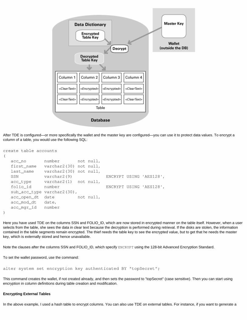
After TDE is configured—or more specifically the wallet and the master key are configured—you can use it to protect data values. To encrypt a column of a table, you would use the following SQL:

create table accounts( acc_no number not null, first_name varchar2(30) not null, last_name varchar2(30) not null, SSN varchar2(9) ENCRYPT USING 'AES128', acc_type varchar2(1) not null, folio_id number ENCRYPT USING 'AES128', sub_acc_type varchar2(30), acc_open_dt date not null, acc_mod_dt date, acc_mgr_id number)

Here you have used TDE on the columns SSN and FOLIO_ID, which are now stored in encrypted manner on the table itself. However, when a user selects from the table, she sees the data in clear text because the decryption is performed during retrieval. If the disks are stolen, the information contained in the table segments remain encrypted. The thief needs the table key to see the encrypted value, but to get that he needs the master key, which is externally stored and hence unavailable.

Note the clauses after the columns SSN and FOLIO_ID, which specify ENCRYPT using the 128-bit Advanced Encryption Standard.

To set the wallet password, use the command:

alter system set encryption key authenticated BY "topSecret";

This command creates the wallet, if not created already, and then sets the password to "topSecret" (case sensitive). Then you can start using encryption in column definitions during table creation and modification.

Encrypting External Tables

In the above example, I used a hash table to encrypt columns. You can also use TDE on external tables. For instance, if you want to generate a

dump file containing the data from ACCOUNTS for shipping to a different location, you can use the simple ENCRYPT clause.

create table account_extorganization external( type oracle_datapump default directory dump_dir location ('accounts_1_ext.dmp', 'accounts_2_ext.dmp', 'accounts_3_ext.dmp', 'accounts_4_ext.dmp'))parallel 4asselect ACC_NO,FIRST_NAME,LAST_NAME,SSN ENCRYPT IDENTIFIED BY "topSecret",ACC_TYPE,FOLIO_ID ENCRYPT IDENTIFIED BY "topSecret",SUB_ACC_TYPE,ACC_OPEN_DT,ACC_MOD_DTfrom accounts;

In the files accounts_*_ext.dmp, the values of SSN and FOLIO_ID will not be clear text, but encrypted. If you want to use these files as external tables, you have to supply the password as topSecret to read the files.

As you can see here, TDE is a highly desirable complement to (not a substitute for) access control.

Query XML in SQL

XML has long been a de-facto standard for datatype of many applications involving large character content. Recently it has also become a storage layout for other applications, not limited to large content only.

Oracle has provided XML integration with the database since Oracle9i Database. In that release, you could query XML content using many different methods. In Oracle Database 10g Release 2, new XQuery and XMLTable functions make it even easier to query XML contents. (Note: A thorough discussion of the XQuery specification is beyond the bounds of this article; for background, read the Oracle Magazine article "XQuery: A New Way to Search.")

XQuery

First, let's examine the simpler of the two methods: XQuery. Here's an example:

SQL> xquery 2 for $var1 in (1,2,3,4,5,6,7,8,9) 3 let $var2 := $var1 + 1 4 where $var2 < 6 5 order by $var2 descending 6 return $var2 7 / Result Sequence------------------543

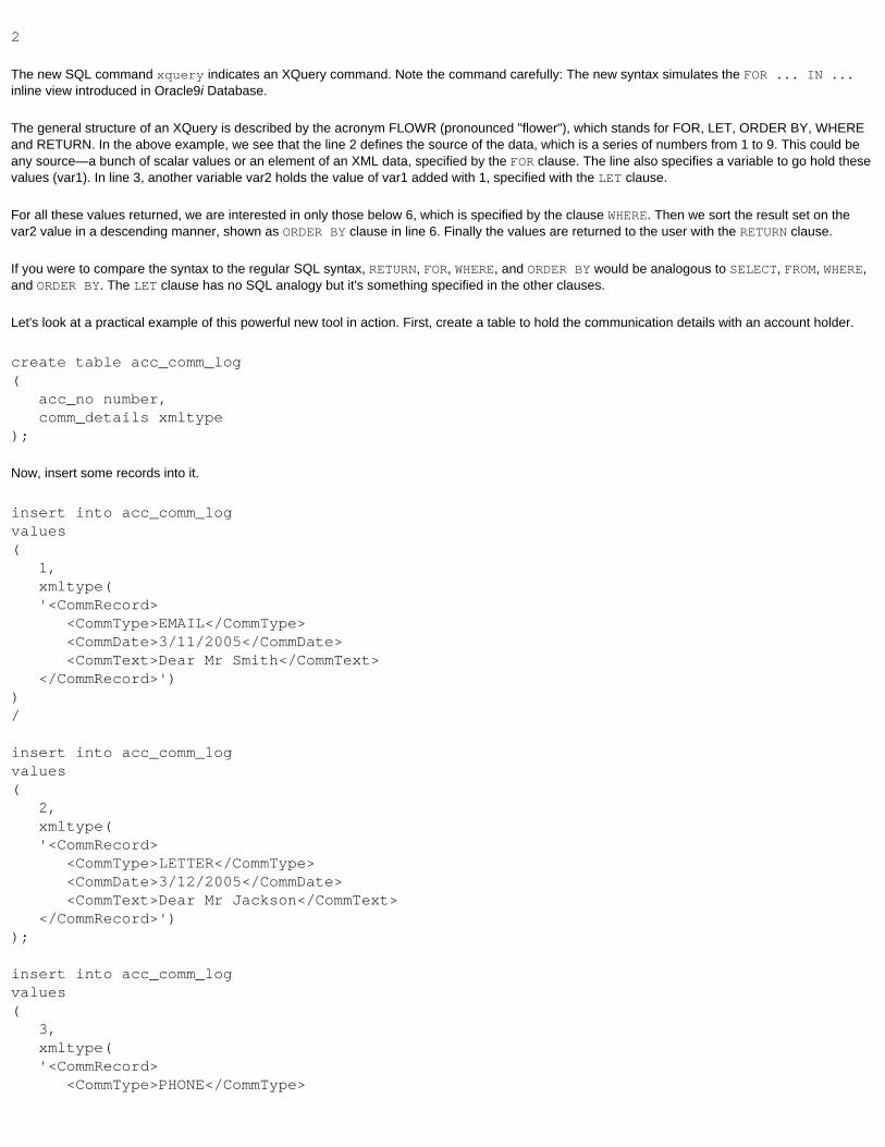
2

The new SQL command xquery indicates an XQuery command. Note the command carefully: The new syntax simulates the FOR ... IN ... inline view introduced in Oracle9i Database.

The general structure of an XQuery is described by the acronym FLOWR (pronounced "flower"), which stands for FOR, LET, ORDER BY, WHERE and RETURN. In the above example, we see that the line 2 defines the source of the data, which is a series of numbers from 1 to 9. This could be any source—a bunch of scalar values or an element of an XML data, specified by the FOR clause. The line also specifies a variable to go hold these values (var1). In line 3, another variable var2 holds the value of var1 added with 1, specified with the LET clause.

For all these values returned, we are interested in only those below 6, which is specified by the clause WHERE. Then we sort the result set on the var2 value in a descending manner, shown as ORDER BY clause in line 6. Finally the values are returned to the user with the RETURN clause.

If you were to compare the syntax to the regular SQL syntax, RETURN, FOR, WHERE, and ORDER BY would be analogous to SELECT, FROM, WHERE, and ORDER BY. The LET clause has no SQL analogy but it's something specified in the other clauses.

Let's look at a practical example of this powerful new tool in action. First, create a table to hold the communication details with an account holder.

create table acc_comm_log ( acc_no number, comm_details xmltype);

Now, insert some records into it.

insert into acc_comm_logvalues( 1, xmltype( '<CommRecord> <CommType>EMAIL</CommType> <CommDate>3/11/2005</CommDate> <CommText>Dear Mr Smith</CommText> </CommRecord>'))/

insert into acc_comm_logvalues( 2, xmltype( '<CommRecord> <CommType>LETTER</CommType> <CommDate>3/12/2005</CommDate> <CommText>Dear Mr Jackson</CommText> </CommRecord>'));

insert into acc_comm_logvalues( 3, xmltype( '<CommRecord> <CommType>PHONE</CommType>

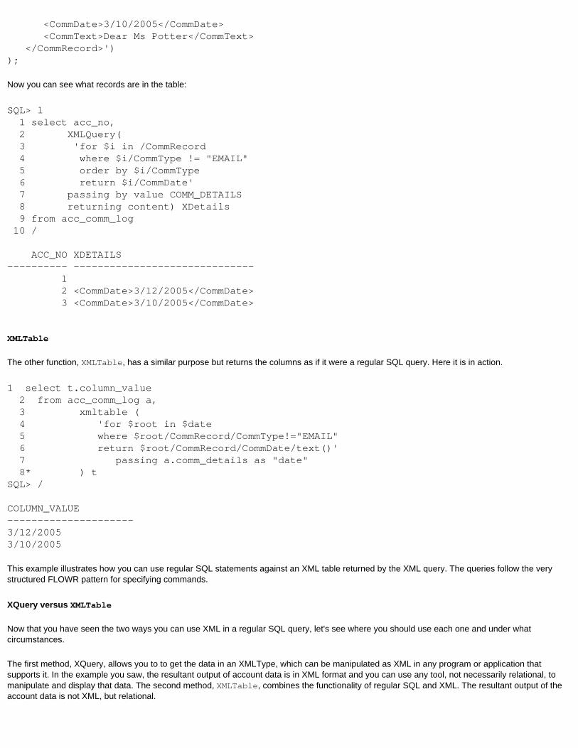
<CommDate>3/10/2005</CommDate> <CommText>Dear Ms Potter</CommText> </CommRecord>'));

Now you can see what records are in the table:

SQL> l 1 select acc_no, 2 XMLQuery( 3 'for $i in /CommRecord 4 where $i/CommType != "EMAIL" 5 order by $i/CommType 6 return $i/CommDate' 7 passing by value COMM_DETAILS 8 returning content) XDetails 9 from acc_comm_log 10 / ACC_NO XDETAILS---------- ------------------------------ 1 2 <CommDate>3/12/2005</CommDate> 3 <CommDate>3/10/2005</CommDate>

XMLTable

The other function, XMLTable, has a similar purpose but returns the columns as if it were a regular SQL query. Here it is in action.

1 select t.column_value 2 from acc_comm_log a, 3 xmltable ( 4 'for $root in $date 5 where $root/CommRecord/CommType!="EMAIL" 6 return $root/CommRecord/CommDate/text()' 7 passing a.comm_details as "date" 8* ) tSQL> / COLUMN_VALUE---------------------3/12/20053/10/2005

This example illustrates how you can use regular SQL statements against an XML table returned by the XML query. The queries follow the very structured FLOWR pattern for specifying commands.

XQuery versus XMLTable

Now that you have seen the two ways you can use XML in a regular SQL query, let's see where you should use each one and under what circumstances.

The first method, XQuery, allows you to to get the data in an XMLType, which can be manipulated as XML in any program or application that supports it. In the example you saw, the resultant output of account data is in XML format and you can use any tool, not necessarily relational, to manipulate and display that data. The second method, XMLTable, combines the functionality of regular SQL and XML. The resultant output of the account data is not XML, but relational.

Note that the source in both cases is XML, but XQuery presents the data in XML format using XMLType whereas XMLTable presents it as a relational table, which can be manipulated as a regular table. This functionality may work best for existing programs which expect a table, while bringing the power of XML into the mix.

XML is quite useful where the exact structure of the data is not well known in advance. In the example above, the communication records are different based on the mode. If it's email, then the attributes could be email address of the recipient, return address, any carbon copies (cc:, bcc:, and so on), the text of the message and so on. If it's a phone call, the attributes are phone number called, the type of number (home, work, cell, and so on), the person answered, the voicemail left, and so on. If you were to design a table that holds all possible types of attributes, it would span across many columns and may become tedious to read. However, if you just have one column as XMLType, then you can cram everything there but still retain the unique attributes of the communication type. The query can still use a simple SQL interface, making application development a breeze.

For more information about Oracle's implementation of XQuery, visit the Oracle XQuery page on OTN.

Enhanced COMMIT

When a session commits, the redo log buffer is flushed to the online redo logs on disk. This process ensures that transactions can be replayed from the redo logs if necessary when recovery is performed on the database.

Sometimes, however, you may want to trade-off the guaranteed ability to recover for better performance. With Oracle Database 10g Release 2, you now have control over how the redo stream is written to the online log files. You can control this behavior while issuing the commit statement itself, or simply make change the default behavior of the database.

Let's see how the commit statement works. After a transaction, when you issue COMMIT, you can have an additional clause:

COMMIT WRITE <option>

where the <option> is what influences the redo stream. The option WAIT is the default behavior. For instance, you can issue:

COMMIT WRITE WAIT;

This command has the same effect as COMMIT itself. The commit does not get the control back to the user until the redo stream is written to the online redo log files. If you don't want it to wait, you could issue:

COMMIT WRITE NOWAIT;

In this case, the control immediately returns to the session, even before the redo streams are written to the online redo logs.

When a commit is issued, the Log Writer process writes the redo stream to the online redo logs. If you are making a series of transactions, such as in a batch processing environment, you may not want it to commit so frequently. Of course, the best course of action is to change the application to reduce the number of commits; but that may be easier said than done. In that case, you could simply issue the following commit statement:

COMMIT WRITE BATCH;

This command will make the commit write the redo streams to the log file in batches, instead of at each commit. You can use this technique to reduce log-buffer flushing in a frequent-commit environment. If you want to write the log buffer immediately, you would issue:

COMMIT WRITE IMMEDIATE;

If you want a specific commit behavior to be the default for a database, you could issue the following statement.

ALTER SYSTEM SET COMMIT_WRITE = NOWAIT;

This command will make this behavior the default across the database. You can also make it at session level:

ALTER SESSION SET COMMIT_WORK = NOWAIT;

As with any parameter, the parameter behaves the setting at the system level, if set. If there is a setting at the session level, the session level

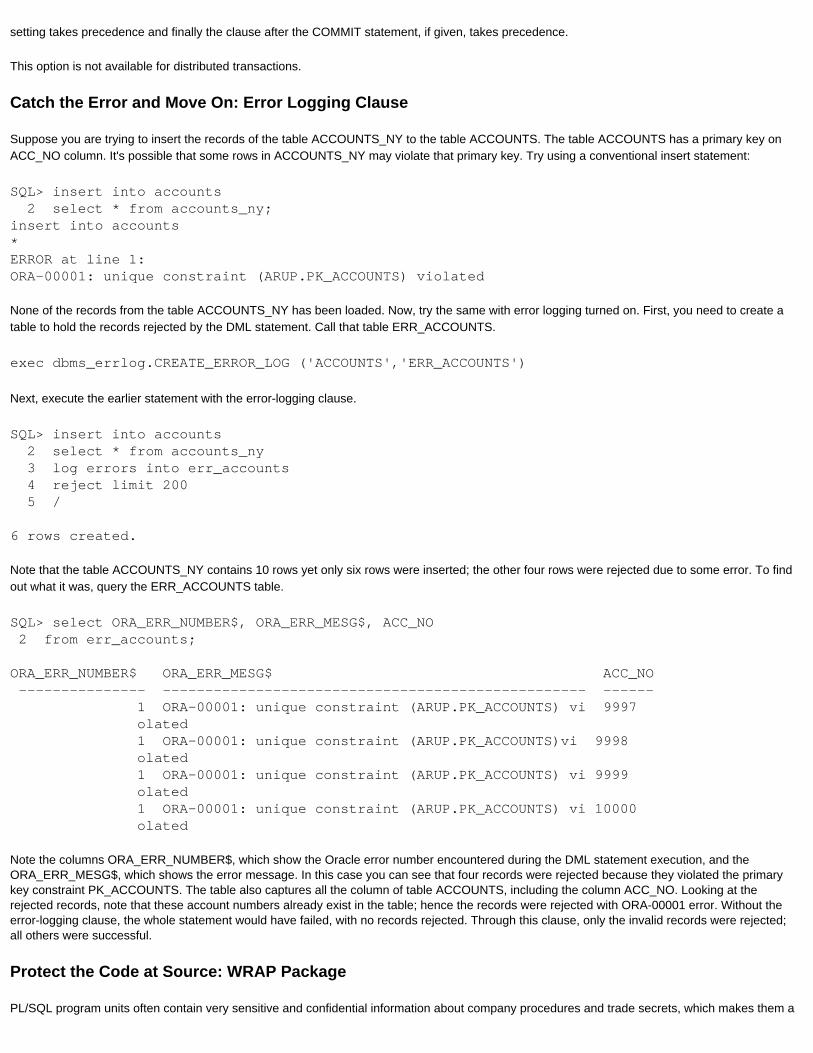
setting takes precedence and finally the clause after the COMMIT statement, if given, takes precedence.

This option is not available for distributed transactions.

Catch the Error and Move On: Error Logging Clause

Suppose you are trying to insert the records of the table ACCOUNTS_NY to the table ACCOUNTS. The table ACCOUNTS has a primary key on ACC_NO column. It's possible that some rows in ACCOUNTS_NY may violate that primary key. Try using a conventional insert statement:

SQL> insert into accounts 2 select * from accounts_ny;insert into accounts*ERROR at line 1:ORA-00001: unique constraint (ARUP.PK_ACCOUNTS) violated

None of the records from the table ACCOUNTS_NY has been loaded. Now, try the same with error logging turned on. First, you need to create a table to hold the records rejected by the DML statement. Call that table ERR_ACCOUNTS.

exec dbms_errlog.CREATE_ERROR_LOG ('ACCOUNTS','ERR_ACCOUNTS')

Next, execute the earlier statement with the error-logging clause.

SQL> insert into accounts 2 select * from accounts_ny 3 log errors into err_accounts 4 reject limit 200 5 /

6 rows created.

Note that the table ACCOUNTS_NY contains 10 rows yet only six rows were inserted; the other four rows were rejected due to some error. To find out what it was, query the ERR_ACCOUNTS table.

SQL> select ORA_ERR_NUMBER$, ORA_ERR_MESG$, ACC_NO 2 from err_accounts;

ORA_ERR_NUMBER$ ORA_ERR_MESG$ ACC_NO --------------- -------------------------------------------------- ------ 1 ORA-00001: unique constraint (ARUP.PK_ACCOUNTS) vi 9997 olated 1 ORA-00001: unique constraint (ARUP.PK_ACCOUNTS)vi 9998 olated 1 ORA-00001: unique constraint (ARUP.PK_ACCOUNTS) vi 9999 olated 1 ORA-00001: unique constraint (ARUP.PK_ACCOUNTS) vi 10000 olated

Note the columns ORA_ERR_NUMBER$, which show the Oracle error number encountered during the DML statement execution, and the ORA_ERR_MESG$, which shows the error message. In this case you can see that four records were rejected because they violated the primary key constraint PK_ACCOUNTS. The table also captures all the column of table ACCOUNTS, including the column ACC_NO. Looking at the rejected records, note that these account numbers already exist in the table; hence the records were rejected with ORA-00001 error. Without the error-logging clause, the whole statement would have failed, with no records rejected. Through this clause, only the invalid records were rejected; all others were successful.

Protect the Code at Source: WRAP Package

PL/SQL program units often contain very sensitive and confidential information about company procedures and trade secrets, which makes them a

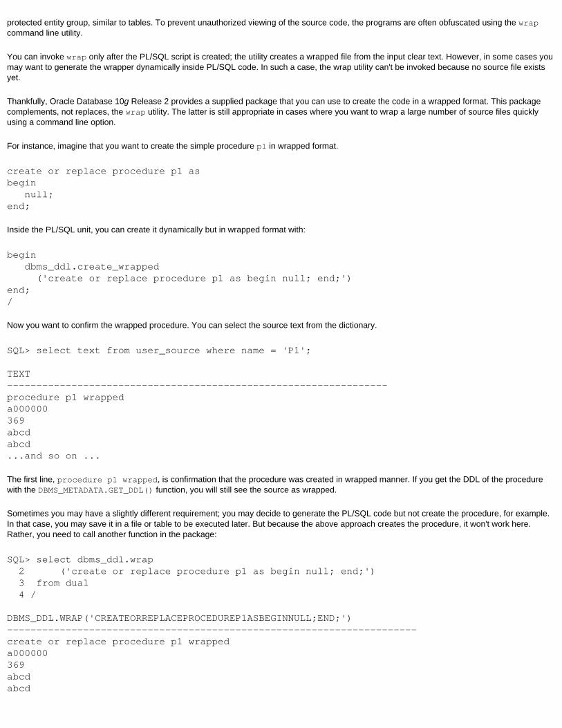
protected entity group, similar to tables. To prevent unauthorized viewing of the source code, the programs are often obfuscated using the wrap command line utility.

You can invoke wrap only after the PL/SQL script is created; the utility creates a wrapped file from the input clear text. However, in some cases you may want to generate the wrapper dynamically inside PL/SQL code. In such a case, the wrap utility can't be invoked because no source file exists yet.

Thankfully, Oracle Database 10g Release 2 provides a supplied package that you can use to create the code in a wrapped format. This package complements, not replaces, the wrap utility. The latter is still appropriate in cases where you want to wrap a large number of source files quickly using a command line option.

For instance, imagine that you want to create the simple procedure p1 in wrapped format.

create or replace procedure p1 as begin null; end;

Inside the PL/SQL unit, you can create it dynamically but in wrapped format with:

begin dbms_ddl.create_wrapped ('create or replace procedure p1 as begin null; end;')end;/

Now you want to confirm the wrapped procedure. You can select the source text from the dictionary.

SQL> select text from user_source where name = 'P1';

TEXT-----------------------------------------------------------------procedure p1 wrappeda000000369abcdabcd...and so on ...

The first line, procedure p1 wrapped, is confirmation that the procedure was created in wrapped manner. If you get the DDL of the procedure with the DBMS_METADATA.GET_DDL() function, you will still see the source as wrapped.

Sometimes you may have a slightly different requirement; you may decide to generate the PL/SQL code but not create the procedure, for example. In that case, you may save it in a file or table to be executed later. But because the above approach creates the procedure, it won't work here. Rather, you need to call another function in the package:

SQL> select dbms_ddl.wrap 2 ('create or replace procedure p1 as begin null; end;') 3 from dual 4 /

DBMS_DDL.WRAP('CREATEORREPLACEPROCEDUREP1ASBEGINNULL;END;')----------------------------------------------------------------------create or replace procedure p1 wrappeda000000369abcdabcd

... and so on ...

The output of the WRAP function is the wrapped output of the PL/SQL code passed as a parameter. This parameter can be stored in a flat file or a table and executed later. This comes in handy in situations where you generate the code to be deployed elsewhere and the security of the code cannot compromised in any way.

The above approach works fine as long as you can pass the entire text of the stored code as a varchar2 datatype, which is limited to 32K. If the PL/SQL code exceeds 32K, you have to use a slightly different method: accept a collection variable as the input.

Here you can use a supplied datatype: varchar2s in the package DBMS_SQL. This is a collection datatype (TABLE OF VARCHAR2), with each element of the table accepting up to 32K of text; you can extend it to as many elements as necessary. Suppose, for example, that you have to wrap a very long procedure called myproc, which is defined as follows:

create or replace procedure myproc as l_key VARCHAR2(200);begin l_key := 'ARUPNANDA';end;

Of course, this is not a very long procedure at all; but for demonstration purposes assume it is. To create it as wrapped, you would execute the following PL/SQL block:

1 declare2 l_input_code dbms_sql.varchar2s;3 begin4 l_input_code (1) := 'Array to hold the MYPROC';5 l_input_code (2) := 'create or replace procedure myproc as ';6 l_input_code (3) := ' l_key VARCHAR2(200);';7 l_input_code (4) := 'begin ';8 l_input_code (5) := ' l_key := ''ARUPNANDA'';';9 l_input_code (6) := 'end;';10 l_input_code (7) := 'the end';11 sys.dbms_ddl.create_wrapped (12 ddl => l_input_code,13 lb => 2,14 ub => 615 );16* end;

Here we have defined a variable, l_input_code, to hold the input clear text code. In lines 4 through 10, we have populated the lines with the code we are going to wrap. In this example, for the same of simplicity, I have used very small lines. In reality, you may be forced to use quite long lines, up to 32KB in size. Similarly, I have used only 7 elements in the array; in reality you may be use several to fit the entire code.

Lines 11 through 15 show how I have called the procedure to create the procedure as wrapped. I have passed the collection as a parameter DDL, in line 12. But, take a pause here—I have assigned a comment as the first element of the array, perhaps for documentation. It's not a valid syntax, however. Similarly, I assigned another comment to the last element (7) of the array, again not a valid syntax for creating a procedure. To let the wrapping work on only the valid lines, I have specified the lowest (2) and highest elements (6) of the collection that stores our code in lines 13 and 14. The parameter LB shows the lower bound of the array, which is 2 in our example, and HB, the higher bound (6).

As you can see, using this approach, you can now create any sized procedure in wrapped format from within your PL/SQL code.

Conditional Compilation in PL/SQL: Write Once, Execute Many

Many of you have worked with the C language, which supports the concept of compiler directives. In C programs, depending on the version of the compiler involved, the value of certain variables may differ.

In Oracle Database 10g Release 2, PL/SQL has a similar feature: pre-processor directives can now be provided that are evaluated during compilation, not runtime. For example, let's create a very simple function that returns a string.

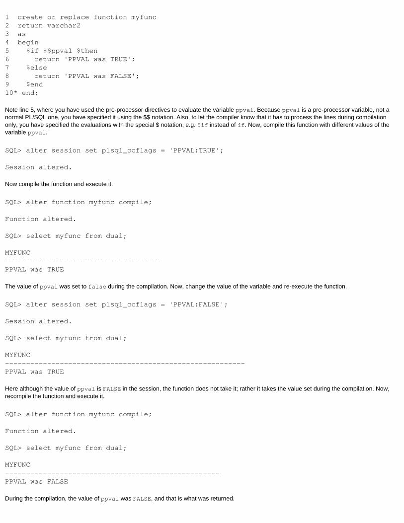
1 create or replace function myfunc2 return varchar23 as4 begin5 $if $$ppval $then6 return 'PPVAL was TRUE';7 $else8 return 'PPVAL was FALSE';9 $end10* end;

Note line 5, where you have used the pre-processor directives to evaluate the variable ppval. Because ppval is a pre-processor variable, not a normal PL/SQL one, you have specified it using the $$ notation. Also, to let the compiler know that it has to process the lines during compilation only, you have specified the evaluations with the special $ notation, e.g. $if instead of if. Now, compile this function with different values of the variable ppval.

SQL> alter session set plsql_ccflags = 'PPVAL:TRUE';

Session altered.

Now compile the function and execute it.

SQL> alter function myfunc compile;

Function altered.

SQL> select myfunc from dual;

MYFUNC-------------------------------------PPVAL was TRUE

The value of ppval was set to false during the compilation. Now, change the value of the variable and re-execute the function.

SQL> alter session set plsql_ccflags = 'PPVAL:FALSE';

Session altered.

SQL> select myfunc from dual;

MYFUNC---------------------------------------------------------PPVAL was TRUE

Here although the value of ppval is FALSE in the session, the function does not take it; rather it takes the value set during the compilation. Now, recompile the function and execute it.

SQL> alter function myfunc compile;

Function altered.

SQL> select myfunc from dual;

MYFUNC---------------------------------------------------PPVAL was FALSE

During the compilation, the value of ppval was FALSE, and that is what was returned.

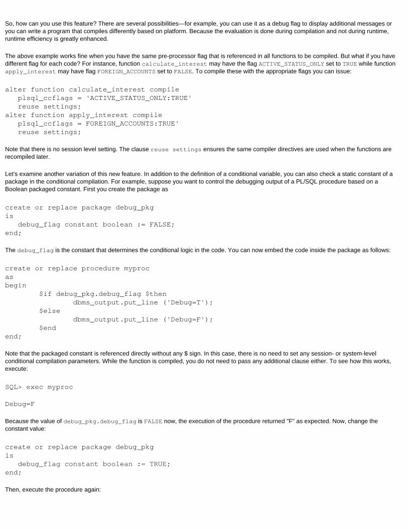
So, how can you use this feature? There are several possibilities—for example, you can use it as a debug flag to display additional messages or you can write a program that compiles differently based on platform. Because the evaluation is done during compilation and not during runtime, runtime efficiency is greatly enhanced.

The above example works fine when you have the same pre-processor flag that is referenced in all functions to be compiled. But what if you have different flag for each code? For instance, function calculate_interest may have the flag ACTIVE_STATUS_ONLY set to TRUE while function apply_interest may have flag FOREIGN_ACCOUNTS set to FALSE. To compile these with the appropriate flags you can issue:

alter function calculate_interest compile plsql_ccflags = 'ACTIVE_STATUS_ONLY:TRUE' reuse settings;alter function apply_interest compile plsql_ccflags = FOREIGN_ACCOUNTS:TRUE' reuse settings;

Note that there is no session level setting. The clause reuse settings ensures the same compiler directives are used when the functions are recompiled later.

Let's examine another variation of this new feature. In addition to the definition of a conditional variable, you can also check a static constant of a package in the conditional compilation. For example, suppose you want to control the debugging output of a PL/SQL procedure based on a Boolean packaged constant. First you create the package as

create or replace package debug_pkgis debug_flag constant boolean := FALSE;end;

The debug_flag is the constant that determines the conditional logic in the code. You can now embed the code inside the package as follows:

create or replace procedure myprocasbegin $if debug_pkg.debug_flag $then dbms_output.put_line ('Debug=T'); $else dbms_output.put_line ('Debug=F'); $endend;

Note that the packaged constant is referenced directly without any $ sign. In this case, there is no need to set any session- or system-level conditional compilation parameters. While the function is compiled, you do not need to pass any additional clause either. To see how this works, execute:

SQL> exec myproc

Debug=F

Because the value of debug_pkg.debug_flag is FALSE now, the execution of the procedure returned "F" as expected. Now, change the constant value:

create or replace package debug_pkgis debug_flag constant boolean := TRUE;end;

Then, execute the procedure again:

SQL> exec myproc

Debug=T

The procedure picked up the value of the constant to show "T," as expected. Note a very important difference here—you did not need to recompile the procedure; the change to the constant was picked up automatically!

Unlimited DBMS Output

Remember the dreaded error that resembles the following lines?

ERROR at line 1:ORA-20000: ORU-10027: buffer overflow, limit of 1000000 bytesORA-06512: at "SYS.DBMS_OUTPUT", line 32ORA-06512: at "SYS.DBMS_OUTPUT", line 97ORA-06512: at "SYS.DBMS_OUTPUT", line 112ORA-06512: at line 2

It is due to the fact that the maximum possible characters handled by the supplied package dbms_output used to be 1 million bytes. In Oracle Database 10g Release 2,, that restriction has been lifted: The maximum output can now be as much as required. You can set it to "unlimited" by simply issuing

set serveroutput on

The above statement produces the following result:

SQL> show serveroutputserveroutput ON size 2000 format WORD_WRAPPED

Note how the default value of the maximum size of the output used to be 2,000. In Oracle Database 10g Release 2, the command shows the following result:

SQL> show serveroutputserveroutput ON SIZE UNLIMITED FORMAT WORD_WRAPPED

The default value is UNLIMITED.

Another inconvenience was the maximum size of a line displayed by dbms_output. The following is a typical error message for lines longer than 255 bytes.

ERROR at line 1:ORA-20000: ORU-10028: line length overflow, limit of 255 chars per lineORA-06512: at "SYS.DBMS_OUTPUT", line 35ORA-06512: at "SYS.DBMS_OUTPUT", line 115ORA-06512: at line 2

In Oracle Database 10g Release 2, the lines can be of any length.

In Part 2, I'll cover manageability features.

Part 2: Manageability Features

The Self-Managing Database becomes even more so with an Automatic Storage Management command-line tool, direct-attached SGA access, support for online partition redefinition, and more.

Covered in This Installment: · ASM Command Line Tool· Drop Empty Datafiles· Direct SGA Access for Hung/Slow Systems· Redefine a Partition Online· Block Integrity Checking in Memory, Not Just on Disk· Online Limit Changes· Faster Startup· Managing Multiple Objects in Oracle Enterprise Manager· Automatic Segment Advisor· Event-Based Scheduling

ASM Command Line Tool

Oracle Automatic Storage Management (ASM; see Part 1 of this series), a specialized filesystem introduced in Oracle Database 10g Release 1, brings much-needed support for the management of datafiles.

ASM is administered through SQL commands or, if necessary, the Oracle Enterprise Manager interface. Similarly, it is visible through the SQL interface or the GUI. This approach is fine for most DBAs, but some sysadmins unfamiliar with SQL do not like the idea of learning SQL. And as a DBA, you probably aren't comfortable giving access to Oracle Enterprise Manager to non-DBAs.

In Oracle Database 10g Release 2, a new ASM command line tool bridges that gap. This interface, called asmcmd, lets you do a lot of things with the datafiles stored in ASM diskgroups, which are akin to filesystems and corresponding files. The tool is based on Perl, so the latter needs to be in the path. If the path to Perl is not set properly, you may want to create a soft link to the directory where Perl exists, or just modify the file asmcmd to reflect the correct path of the Perl executable.

Remember to set the ORACLE_SID to the ASM instance (typically +ASM), not the actual database instance running on the server. Invoke the command by typing

asmcmd -p

The -p option enables the display the current path in the prompt.

Now try some very simple commands. After raising the command line prompt (ASMCMD >), type ls to see all the mounted diskgroups.

ASMCMD [+] > lsDGROUP1/DGROUP10/DGROUP2/DGROUP3/DGROUP4/DGROUP5/DGROUP6/DGROUP7/DGROUP8/DGROUP9/

You can see all the diskgroups created and mounted in the ASM instance (DGROUP1 through DGROUP10) here.

Now explore the diskgroup DGROUP1. You can make changes to the disk group much like changing a directory, using the cd command.

ASMCMD [+] > cd dgroup1

You can even go down to the parent directory by typing cd .., as you would in UNIX-like OSs or even Windows. Now, confirm which files have been created in that diskgroup.

ASMCMD [+dgroup1] > lsORCL/

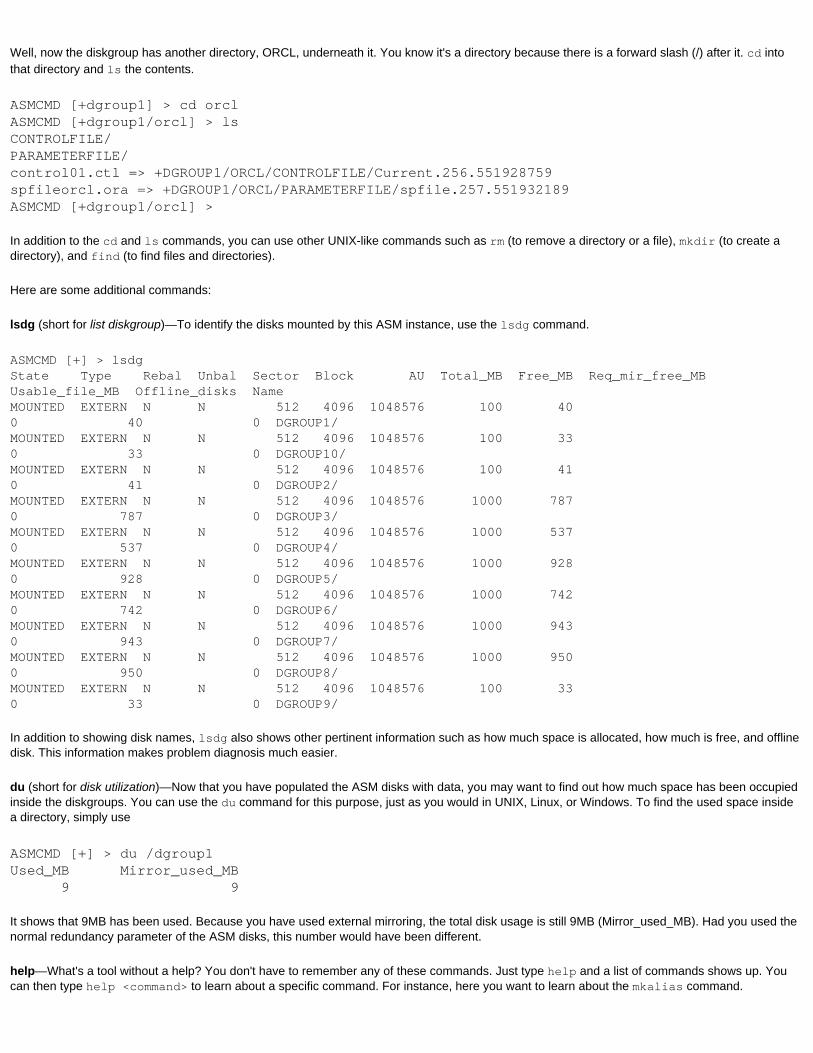
Well, now the diskgroup has another directory, ORCL, underneath it. You know it's a directory because there is a forward slash (/) after it. cd into that directory and ls the contents.

ASMCMD [+dgroup1] > cd orclASMCMD [+dgroup1/orcl] > lsCONTROLFILE/PARAMETERFILE/control01.ctl => +DGROUP1/ORCL/CONTROLFILE/Current.256.551928759spfileorcl.ora => +DGROUP1/ORCL/PARAMETERFILE/spfile.257.551932189ASMCMD [+dgroup1/orcl] >

In addition to the cd and ls commands, you can use other UNIX-like commands such as rm (to remove a directory or a file), mkdir (to create a directory), and find (to find files and directories).

Here are some additional commands:

lsdg (short for list diskgroup)—To identify the disks mounted by this ASM instance, use the lsdg command.

ASMCMD [+] > lsdgState Type Rebal Unbal Sector Block AU Total_MB Free_MB Req_mir_free_MB Usable_file_MB Offline_disks NameMOUNTED EXTERN N N 512 4096 1048576 100 40 0 40 0 DGROUP1/MOUNTED EXTERN N N 512 4096 1048576 100 33 0 33 0 DGROUP10/MOUNTED EXTERN N N 512 4096 1048576 100 41 0 41 0 DGROUP2/MOUNTED EXTERN N N 512 4096 1048576 1000 787 0 787 0 DGROUP3/MOUNTED EXTERN N N 512 4096 1048576 1000 537 0 537 0 DGROUP4/MOUNTED EXTERN N N 512 4096 1048576 1000 928 0 928 0 DGROUP5/MOUNTED EXTERN N N 512 4096 1048576 1000 742 0 742 0 DGROUP6/MOUNTED EXTERN N N 512 4096 1048576 1000 943 0 943 0 DGROUP7/MOUNTED EXTERN N N 512 4096 1048576 1000 950 0 950 0 DGROUP8/MOUNTED EXTERN N N 512 4096 1048576 100 33 0 33 0 DGROUP9/

In addition to showing disk names, lsdg also shows other pertinent information such as how much space is allocated, how much is free, and offline disk. This information makes problem diagnosis much easier.

du (short for disk utilization)—Now that you have populated the ASM disks with data, you may want to find out how much space has been occupied inside the diskgroups. You can use the du command for this purpose, just as you would in UNIX, Linux, or Windows. To find the used space inside a directory, simply use

ASMCMD [+] > du /dgroup1Used_MB Mirror_used_MB 9 9

It shows that 9MB has been used. Because you have used external mirroring, the total disk usage is still 9MB (Mirror_used_MB). Had you used the normal redundancy parameter of the ASM disks, this number would have been different.

help—What's a tool without a help? You don't have to remember any of these commands. Just type help and a list of commands shows up. You can then type help <command> to learn about a specific command. For instance, here you want to learn about the mkalias command.

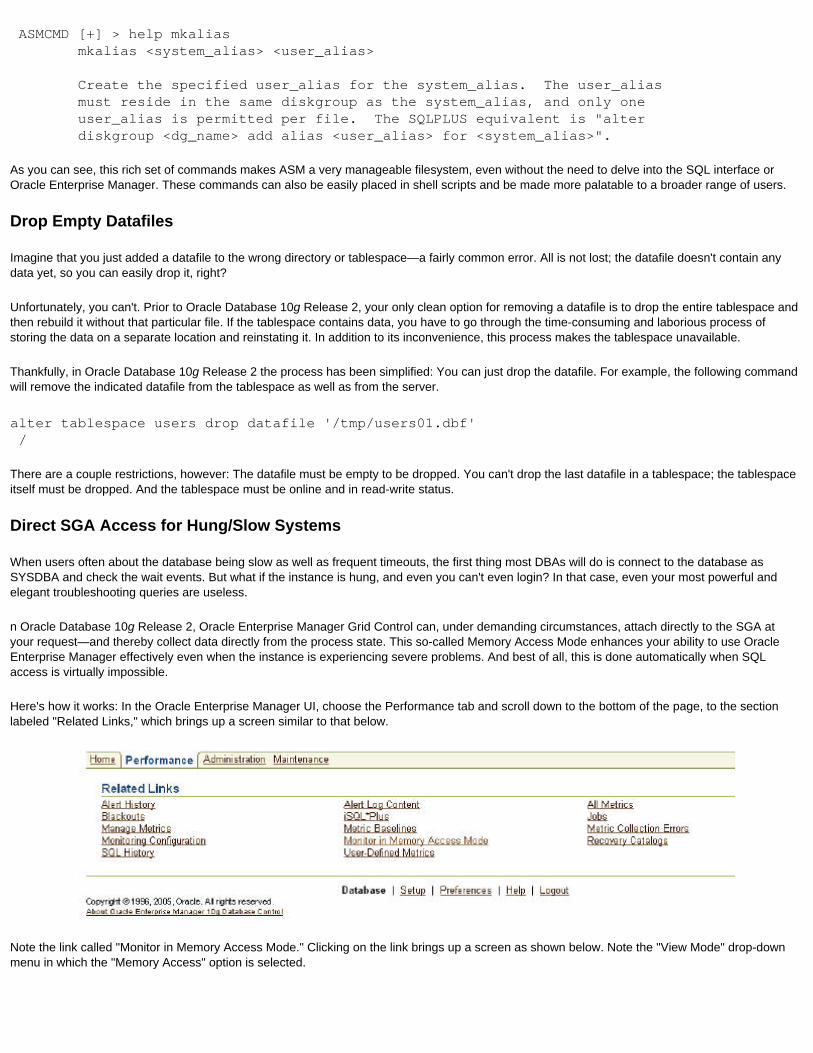
ASMCMD [+] > help mkalias mkalias <system_alias> <user_alias> Create the specified user_alias for the system_alias. The user_alias must reside in the same diskgroup as the system_alias, and only one user_alias is permitted per file. The SQLPLUS equivalent is "alter diskgroup <dg_name> add alias <user_alias> for <system_alias>".

As you can see, this rich set of commands makes ASM a very manageable filesystem, even without the need to delve into the SQL interface or Oracle Enterprise Manager. These commands can also be easily placed in shell scripts and be made more palatable to a broader range of users.

Drop Empty Datafiles

Imagine that you just added a datafile to the wrong directory or tablespace—a fairly common error. All is not lost; the datafile doesn't contain any data yet, so you can easily drop it, right?

Unfortunately, you can't. Prior to Oracle Database 10g Release 2, your only clean option for removing a datafile is to drop the entire tablespace and then rebuild it without that particular file. If the tablespace contains data, you have to go through the time-consuming and laborious process of storing the data on a separate location and reinstating it. In addition to its inconvenience, this process makes the tablespace unavailable.

Thankfully, in Oracle Database 10g Release 2 the process has been simplified: You can just drop the datafile. For example, the following command will remove the indicated datafile from the tablespace as well as from the server.

alter tablespace users drop datafile '/tmp/users01.dbf' /

There are a couple restrictions, however: The datafile must be empty to be dropped. You can't drop the last datafile in a tablespace; the tablespace itself must be dropped. And the tablespace must be online and in read-write status.

Direct SGA Access for Hung/Slow Systems

When users often about the database being slow as well as frequent timeouts, the first thing most DBAs will do is connect to the database as SYSDBA and check the wait events. But what if the instance is hung, and even you can't even login? In that case, even your most powerful and elegant troubleshooting queries are useless.

n Oracle Database 10g Release 2, Oracle Enterprise Manager Grid Control can, under demanding circumstances, attach directly to the SGA at your request—and thereby collect data directly from the process state. This so-called Memory Access Mode enhances your ability to use Oracle Enterprise Manager effectively even when the instance is experiencing severe problems. And best of all, this is done automatically when SQL access is virtually impossible.

Here's how it works: In the Oracle Enterprise Manager UI, choose the Performance tab and scroll down to the bottom of the page, to the section labeled "Related Links," which brings up a screen similar to that below.

Note the link called "Monitor in Memory Access Mode." Clicking on the link brings up a screen as shown below. Note the "View Mode" drop-down menu in which the "Memory Access" option is selected.

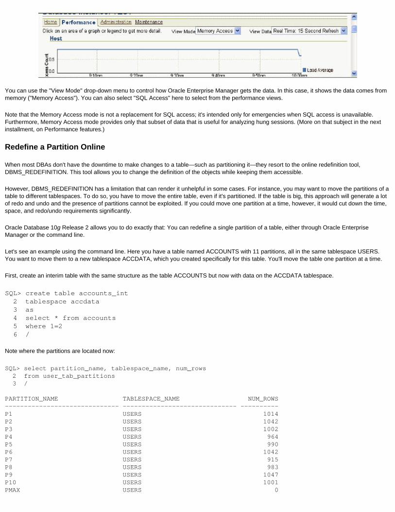
You can use the "View Mode" drop-down menu to control how Oracle Enterprise Manager gets the data. In this case, it shows the data comes from memory ("Memory Access"). You can also select "SQL Access" here to select from the performance views.

Note that the Memory Access mode is not a replacement for SQL access; it's intended only for emergencies when SQL access is unavailable. Furthermore, Memory Access mode provides only that subset of data that is useful for analyzing hung sessions. (More on that subject in the next installment, on Performance features.)

Redefine a Partition Online

When most DBAs don't have the downtime to make changes to a table—such as partitioning it—they resort to the online redefinition tool, DBMS_REDEFINITION. This tool allows you to change the definition of the objects while keeping them accessible.

However, DBMS_REDEFINITION has a limitation that can render it unhelpful in some cases. For instance, you may want to move the partitions of a table to different tablespaces. To do so, you have to move the entire table, even if it's partitioned. If the table is big, this approach will generate a lot of redo and undo and the presence of partitions cannot be exploited. If you could move one partition at a time, however, it would cut down the time, space, and redo/undo requirements significantly.

Oracle Database 10g Release 2 allows you to do exactly that: You can redefine a single partition of a table, either through Oracle Enterprise Manager or the command line.

Let's see an example using the command line. Here you have a table named ACCOUNTS with 11 partitions, all in the same tablespace USERS. You want to move them to a new tablespace ACCDATA, which you created specifically for this table. You'll move the table one partition at a time.

First, create an interim table with the same structure as the table ACCOUNTS but now with data on the ACCDATA tablespace.

SQL> create table accounts_int 2 tablespace accdata 3 as 4 select * from accounts 5 where 1=2 6 /

Note where the partitions are located now:

SQL> select partition_name, tablespace_name, num_rows 2 from user_tab_partitions 3 /

PARTITION_NAME TABLESPACE_NAME NUM_ROWS------------------------------ ------------------------------ ----------P1 USERS 1014P2 USERS 1042P3 USERS 1002P4 USERS 964P5 USERS 990P6 USERS 1042P7 USERS 915P8 USERS 983P9 USERS 1047P10 USERS 1001PMAX USERS 0

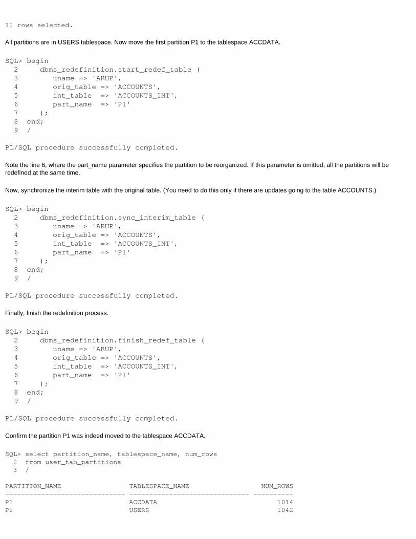
11 rows selected.

All partitions are in USERS tablespace. Now move the first partition P1 to the tablespace ACCDATA.

SQL> begin 2 dbms_redefinition.start_redef_table ( 3 uname => 'ARUP', 4 orig_table => 'ACCOUNTS', 5 int_table => 'ACCOUNTS_INT', 6 part_name => 'P1' 7 ); 8 end; 9 /

PL/SQL procedure successfully completed.

Note the line 6, where the part_name parameter specifies the partition to be reorganized. If this parameter is omitted, all the partitions will be redefined at the same time.

Now, synchronize the interim table with the original table. (You need to do this only if there are updates going to the table ACCOUNTS.)

SQL> begin 2 dbms_redefinition.sync_interim_table ( 3 uname => 'ARUP', 4 orig_table => 'ACCOUNTS', 5 int_table => 'ACCOUNTS_INT', 6 part_name => 'P1' 7 ); 8 end; 9 /

PL/SQL procedure successfully completed.

Finally, finish the redefinition process.

SQL> begin 2 dbms_redefinition.finish_redef_table ( 3 uname => 'ARUP', 4 orig_table => 'ACCOUNTS', 5 int_table => 'ACCOUNTS_INT', 6 part_name => 'P1' 7 ); 8 end; 9 /

PL/SQL procedure successfully completed.

Confirm the partition P1 was indeed moved to the tablespace ACCDATA.

SQL> select partition_name, tablespace_name, num_rows 2 from user_tab_partitions 3 /

PARTITION_NAME TABLESPACE_NAME NUM_ROWS------------------------------ ------------------------------ ----------P1 ACCDATA 1014P2 USERS 1042

P3 USERS 1002P4 USERS 964P5 USERS 990P6 USERS 1042P7 USERS 915P8 USERS 983P9 USERS 1047P10 USERS 1001PMAX USERS 0

11 rows selected.

That's it; repeat the same procedure for other partitions.

In contrast, if you had reorganized the table entirely, you would have (a) required a space equal to the size of the entire table and (b) generated undos for the entire table, which would have to be present—else you would received an error. By doing the process for a single partition, however, you reduced the space requirement to that of a single partition and reduced the undo generation for that partition only.

This powerful and useful feature enables you to reorganize very large objects—as most partitioned objects are—online. Furthermore, note how the statistics are copied to the redefined table as well, as shown in the values of NUM_RWS in the above query; you do not have to regenerate statistics for the newly created table or partitions.

Block Integrity Checking in Memory, Not Just on Disk

An active database instance moves a lot of data around—from the user session to the buffer cache, from the cache to the disk, and vice versa. All these movements can make the data block susceptible to corruption.

Oracle ensures the data block's integrity by computing a checksum on the data value before writing the data block to the disk. This checksum value is also written to the disk. When the block is read from the disk, the reading process calculates the checksum again and then compares against the stored value. If the value is corrupted, the checksums will differ and the corruption revealed.

Because most manipulation occurs in the memory, it might be prudent to perform this check in the source itself, which is the buffer cache. In Oracle Database 10g Release 2, you can make the database perform the check in memory as well by setting the initialization parameter DB_BLOCK_CHECKSUM to FULL.

After this setting Oracle will compute the checksum before any change and compare the checksum to the stored value. This approach uncovers any data corruption in the memory itself and reports errors at that point—which is highly useful for preventing data corruption at the disk level as well as its propagation to the standby database.

Please note that the parameter is set to FALSE by default, unlike the previous releases, where it is set to TRUE.

Online Limit Changes

When you want change parameters defined during the creation of the database, such as MAXDATAFILES, MAXLOGFILES, and so on, what are your options? Prior to Oracle Database 10g Release 2, the only option is to follow these steps:

1. Take a backup of controlfile to trace.2. Modify the parameter you want to change in that trace file.3. Shut the database down.4. Startup Mount.5. Recreate the control file.6. Open the database in RESETLOGS mode.

Needless to say, this approach degrades availability. In addition, because RMAN keeps the metadata about backups in the control file as well as in the catalog, that information is lost during this process. The controlfile is created in RESETLOGS mode, so some backup information may be lost too.

In Oracle Database 10g Release 2, you needn't recreate the control file to change these parameters. Thus, you do not have to lose the RMAN information stored there.

Faster Startup

The days when dinosaurs ruled the earth and 2GB memory was considered large are gone. Now, it's not uncommon to see large buffer caches to the tune of 100GB. When the instance is started, it might take several minutes, or even hours, to initialize a buffer cache of this size.

If you look deeper into the situation, you will notice that the entire buffer cache need not be up when the database instance starts. After the instance starts, the buffer cache is empty, which gradually fills up when users select data from tables. So, there is no need to initialize the entire buffer cache when the instance starts.

In Oracle Database 10g Release 2, this behavior is accounted for in the startup logic. When you start the instance, only 10% of the buffer cache is initialized; the rest is initialized after the database is opened by the checkpoint process. This new approach reduces instance startup time significantly.

Bear in mind, however, that until the entire buffer cache is initialized, automatic buffer cache sizing is not available.

Manage Multiple Objects in Oracle Enterprise Manager

When several objects are invalidated in a schema, what do you generally do? Most likely You create a SQL script that dynamically generates another script that compiles the invalid objects. At least, that is the preferred approach lacking a third-party tool.

But wouldn't it be great if you could use Oracle Enterprise Manager Grid Control for that purpose? Not to just pick an invalid object and click compile, but to actually select several invalid objects at the same time and compile them with one click?

In Oracle Database 10g Release 2, you do have that ability. As shown below, all you have to do is tick the checkboxes next to the objects. Then you can select "Compile" from the drop-down list next to "Actions" to compile all the objects simultaneously.

In addition to compiles, you can do a whole lot of other things such as creating DDL or dropping objects.

Audit Trails in XML Format

If you have been using the built-in auditing tools in Oracle for a long time, you may have noticed that one very useful feature is the ability to write the audit trails to a filesystem. By writing the entries to a filesystem and not the database itself, an additional level of security can be established.

All you have to do is set two initialization parameters:

audit_file_dest = '/auditfs'audit_trail = xml

and restart the instance. These two parameters are not dynamic however; once set, the audit trails will be written to the directory /auditfs. This parameter, audit_file_dest, is optional; the default is $ORACLE_HOME/rdbms/audit directory. These audit trail files will be written as XML files with an .xml extension.

Here is an example of an audit trail in XML format:

- <Audit xmlns="http://xmlns.oracle.com/oracleas/schema/dbserver_audittrail-10_2.xsd" xmlns:xsi="http://www.w3.org/2001/XMLSchema-instance" xsi:schemaLocation="http://xmlns.oracle.com/oracleas/schema/dbserver_audittrail-10_2.xsd"> <Version>10.2</Version> - <AuditRecord> <Audit_Type>8</Audit_Type> <EntryId>1</EntryId> <Extended_Timestamp>2005-03-05T20:52:51.012045</Extended_Timestamp> <DB_User>/</DB_User> <OS_User>oracle</OS_User> <Userhost>oradba</Userhost> <OS_Process>18067</OS_Process> <Terminal>pts/0</Terminal> <Instance_Number>0</Instance_Number> <Returncode>0</Returncode> <OS_Privilege>SYSDBA</OS_Privilege> <Sql_Text>CONNECT</Sql_Text> </AuditRecord> </Audit>

These trace files can easily be parsed by any XML parser to extract useful information from them. You can even load them into the database as XML types and then query them inside SQL, using XML Query as described in Part 1 of this series.

In Oracle Database 10g Release 2, you can combine this XML with a SQL query and select from it as if it were coming from a single SQL source. There is a also a predefined dynamic view V$XML_AUDIT_TRAIL, which selects from the fixed table X$XML_AUDIT_TRAIL. This dynamic view resembles the regular audit trail view DBA_AUDIT_TRAIL in terms structure.

For a DBA, having the audit trail in XML format opens up possibilities for manipulating the files with third-party XML parsers and editors, as well as publishing reports via tools that accept XML as input. You no longer have to write your own parser to interpret the audit trail files.

Automatic Segment Advisor

How do you know which segments have plenty of free space under the high-water mark and would benefit from a reorganization?

You could use the Oracle Enterprise Manager interface provided in Oracle Database 10g to target a specific tablespace to identify potential candidates, but if your database has several hundred tablespaces, you cannot possibly do it every day. Even if you could, not every tablespace would have segments that need reorganization. So wouldn't it be nice to have an automatic tool that proactively scans your segments and reports any potential candidates for reorganization?

In Oracle Database 10g Release 2, the supplied package DBMS_SPACE provides that capability. The built-in function ASA_RECOMMENDATIONS shows the segments; as this is a pipelined function, you will have to use it as follows:

select * from table (dbms_space.asa_recommendations());

The large number of columns will make it difficult to see the output clearly. So, here is just one record shown in vertical format.

TABLESPACE_NAME : USERSSEGMENT_OWNER : ARUPSEGMENT_NAME : ACCOUNTSSEGMENT_TYPE : TABLE PARTITIONPARTITION_NAME : P7

ALLOCATED_SPACE : 0USED_SPACE : 0RECLAIMABLE_SPACE : 0CHAIN_ROWEXCESS : 17RECOMMENDATIONS : The object has chained rows that can be removedby re-org.C1 :C2 :C3 :TASK_ID : 261MESG_ID : 0

Here you'll see that partition P7 of the table ACCOUNTS of the schema ARUP has chained rows. Doing a reorganization will help speed up full table scans in this partition.

This information is collected by an automatically scheduled job that runs in the predefined maintenance window (between 10PM and 6AM on weekdays and between 12 a.m. Saturday and 12 a.m. Monday); you can change those windows using Oracle Enterprise Manager. During this time, the job scans the segments for candidates. If the scan cannot be completed in time, the job is suspended and resumed in the next day's window.

The job stores the information about the segments and tablespaces inspected in a table named wri$_segadv_objlist. You can see the information on the segments inspected in the view DBA_AUTO_SEGADV_CTL.

Event-Based Scheduling

Oracle Scheduler, introduced in Oracle Database 10g Release 1, is the next-generation job scheduling system replacing the DBMS_JOB supplied package. The Scheduler tool has a number of significant advantages over this package, as originally described here.

In the first release of Oracle Scheduler, jobs are based on and triggered on time. But what, for example, if you want to base a trigger on an event? For example, when the Account Manager of an account changes, you may want a batch program to kick in automatically to recompute the revenue and republish the reports.

This type of event-based triggering can be achieved in the Scheduler tool of Oracle Database 10g Release 2. Events are communicated to the Scheduler via Advanced Queueing (AQ), where the payload is an object type. So, first, you need to create an AQ, for instance proc_queue, where any such events will be enqueued. Next, you have to create a schedule based on this event.

begin dbms_scheduler.create_event_schedule ( schedule_name => 'accadmin.acc_mgr_change', start_date => systimestamp, event_condition => 'tab.user_data.event_name = ''acc_mgr_change''', queue_spec => 'proc_queue');end;

Then, you would create a job to follow this schedule. Alternatively you can schedule a job directly without creating a schedule first.

begin dbms_scheduler.create_job ( job_name => acc_mgr_change, program_name => acc_mgr_change_procs, start_date => 'systimestamp, event_condition => 'tab.user_data.event_name = ''acc_mgr_change''', queue_spec => 'proc_queue' enabled => true);end;

The default value is UNLIMITED.

The event-based schedules are very helpful in cases where an event, rather than a specific time, is the determining factor for triggering a job.

In Part 3, I'll cover performance features.

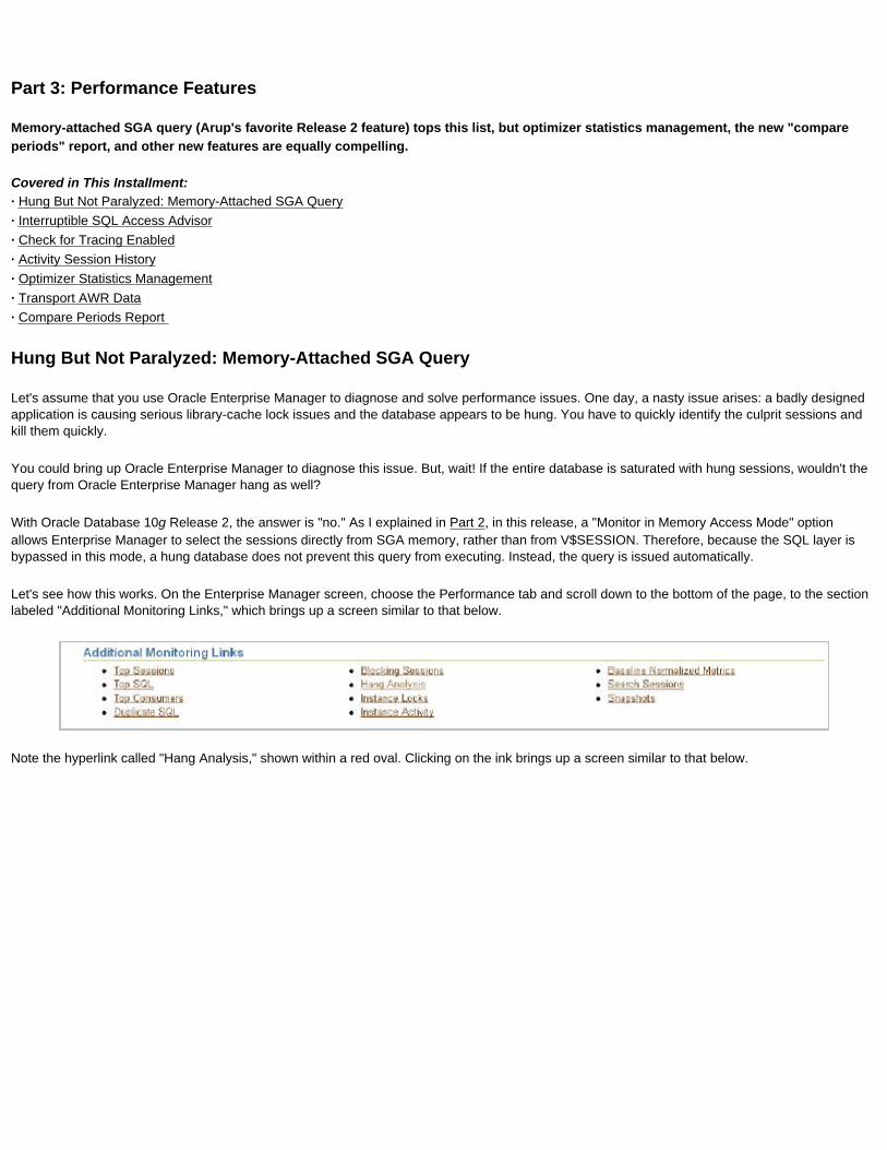
Part 3: Performance Features

Memory-attached SGA query (Arup's favorite Release 2 feature) tops this list, but optimizer statistics management, the new "compare periods" report, and other new features are equally compelling.

Covered in This Installment: · Hung But Not Paralyzed: Memory-Attached SGA Query· Interruptible SQL Access Advisor· Check for Tracing Enabled· Activity Session History· Optimizer Statistics Management· Transport AWR Data· Compare Periods Report

Hung But Not Paralyzed: Memory-Attached SGA Query

Let's assume that you use Oracle Enterprise Manager to diagnose and solve performance issues. One day, a nasty issue arises: a badly designed application is causing serious library-cache lock issues and the database appears to be hung. You have to quickly identify the culprit sessions and kill them quickly.

You could bring up Oracle Enterprise Manager to diagnose this issue. But, wait! If the entire database is saturated with hung sessions, wouldn't the query from Oracle Enterprise Manager hang as well?

With Oracle Database 10g Release 2, the answer is "no." As I explained in Part 2, in this release, a "Monitor in Memory Access Mode" option allows Enterprise Manager to select the sessions directly from SGA memory, rather than from V$SESSION. Therefore, because the SQL layer is bypassed in this mode, a hung database does not prevent this query from executing. Instead, the query is issued automatically.

Let's see how this works. On the Enterprise Manager screen, choose the Performance tab and scroll down to the bottom of the page, to the section labeled "Additional Monitoring Links," which brings up a screen similar to that below.

Note the hyperlink called "Hang Analysis," shown within a red oval. Clicking on the ink brings up a screen similar to that below.

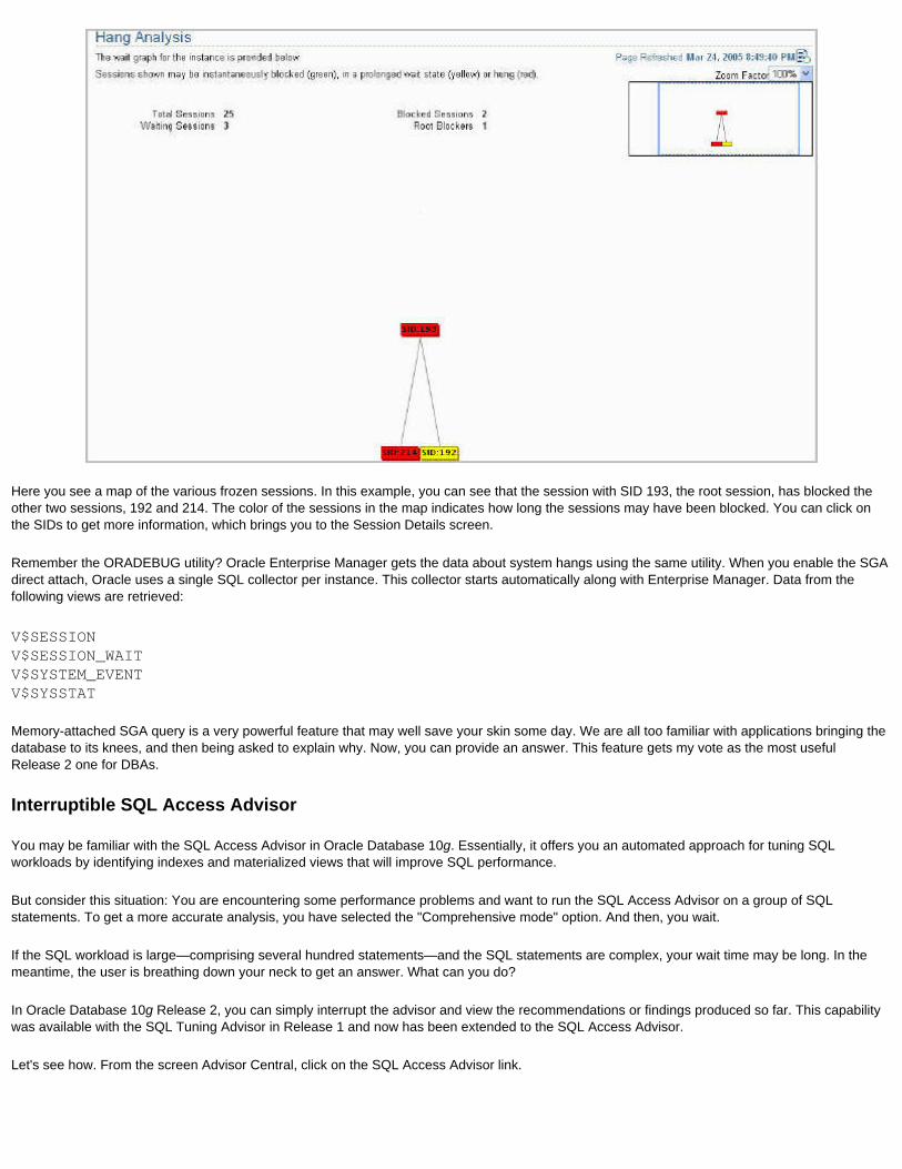
Here you see a map of the various frozen sessions. In this example, you can see that the session with SID 193, the root session, has blocked the other two sessions, 192 and 214. The color of the sessions in the map indicates how long the sessions may have been blocked. You can click on the SIDs to get more information, which brings you to the Session Details screen.

Remember the ORADEBUG utility? Oracle Enterprise Manager gets the data about system hangs using the same utility. When you enable the SGA direct attach, Oracle uses a single SQL collector per instance. This collector starts automatically along with Enterprise Manager. Data from the following views are retrieved:

V$SESSIONV$SESSION_WAITV$SYSTEM_EVENTV$SYSSTAT

Memory-attached SGA query is a very powerful feature that may well save your skin some day. We are all too familiar with applications bringing the database to its knees, and then being asked to explain why. Now, you can provide an answer. This feature gets my vote as the most useful Release 2 one for DBAs.

Interruptible SQL Access Advisor

You may be familiar with the SQL Access Advisor in Oracle Database 10g. Essentially, it offers you an automated approach for tuning SQL workloads by identifying indexes and materialized views that will improve SQL performance.

But consider this situation: You are encountering some performance problems and want to run the SQL Access Advisor on a group of SQL statements. To get a more accurate analysis, you have selected the "Comprehensive mode" option. And then, you wait.

If the SQL workload is large—comprising several hundred statements—and the SQL statements are complex, your wait time may be long. In the meantime, the user is breathing down your neck to get an answer. What can you do?

In Oracle Database 10g Release 2, you can simply interrupt the advisor and view the recommendations or findings produced so far. This capability was available with the SQL Tuning Advisor in Release 1 and now has been extended to the SQL Access Advisor.

Let's see how. From the screen Advisor Central, click on the SQL Access Advisor link.

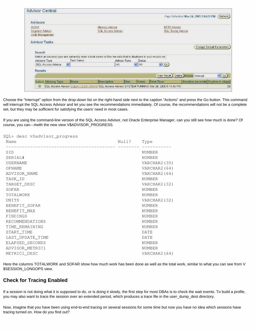
Choose the "Interrupt" option from the drop-down list on the right-hand side next to the caption "Actions" and press the Go button. This command will interrupt the SQL Access Advisor and let you see the recommendations immediately. Of course, the recommendations will not be a complete set, but they may be sufficient for satisfying the users' need in most cases.

If you are using the command-line version of the SQL Access Advisor, not Oracle Enterprise Manager, can you still see how much is done? Of course, you can—#with the new view V$ADVISOR_PROGRESS.

SQL> desc v$advisor_progress Name Null? Type ----------------------------------------- -------- ----------- SID NUMBER SERIAL# NUMBER USERNAME VARCHAR2(30) OPNAME VARCHAR2(64) ADVISOR_NAME VARCHAR2(64) TASK_ID NUMBER TARGET_DESC VARCHAR2(32) SOFAR NUMBER TOTALWORK NUMBER UNITS VARCHAR2(32) BENEFIT_SOFAR NUMBER BENEFIT_MAX NUMBER FINDINGS NUMBER RECOMMENDATIONS NUMBER TIME_REMAINING NUMBER START_TIME DATE LAST_UPDATE_TIME DATE ELAPSED_SECONDS NUMBER ADVISOR_METRIC1 NUMBER METRIC1_DESC VARCHAR2(64)

Here the columns TOTALWORK and SOFAR show how much work has been done as well as the total work, similar to what you can see from V$SESSION_LONGOPS view.

Check for Tracing Enabled

If a session is not doing what it is supposed to do, or is doing it slowly, the first step for most DBAs is to check the wait events. To build a profile, you may also want to trace the session over an extended period, which produces a trace file in the user_dump_dest directory.

Now, imagine that you have been using end-to-end tracing on several sessions for some time but now you have no idea which sessions have tracing turned on. How do you find out?

One way is to sift through the myriad trace files to extract the SID and Serial# columns and match them in the database in V$SESSION view. Needless to say, this process is complex, difficult, and error-prone. But in Oracle Database 10g Release 2, a more elegant, much easier approach is available: All you have to do is to check a view you check anyway, V$SESSION.

Three new columns now show the status of tracing:

● sql_trace—Shows (TRUE/FALSE) if SQL tracing has been enabled in the session ● sql_trace_waits—If session tracing is enabled, you can have the trace write wait information to the trace file; very useful in diagnosing

performance issues. ● sql_trace_binds—If the session uses bind variables, you can have the trace write the bind variable values to the trace file. This column

shows TRUE/FALSE.

When tracing in the session is not turned on, if you select these columns:

select sid, serial#, sql_trace, sql_trace_waits, sql_trace_bindsfrom v$session where username = 'HR'

The output is:

SID SERIAL# SQL_TRAC SQL_T SQL_T---------- ---------- -------- ----- ----- 196 60946 DISABLED FALSE FALSE

Here you can see that tracing is not enabled in the session with SID 196 and Serial# 60946.

Now, you can enable tracing of wait events, but not of bind variables. You can use the package dbms_monitor to enable tracing.

begin dbms_monitor.session_trace_enable ( session_id => 196, serial_num => 60960, waits => true, binds => false );end;/

Now if you want to see the session information:

select sid, serial#, sql_trace, sql_trace_waits, sql_trace_bindsfrom v$session where username = 'HR'

The output is:

SID SERIAL# SQL_TRAC SQL_T SQL_T---------- ---------- -------- ----- ----- 196 60960 ENABLED TRUE FALSE

Note that the view V$SESSION is populated only if the procedure session_trace_enable in the package dbms_monitor is used to enable tracing, not by alter session set sql_trace = true or setting the event 10046. At some point later in time, if you want to find out which sessions have been enabled for tracing, you can do so using the above query.

If you have enabled the trace using the other procedures in the package dbms_monitor—such as SERV_MOD_ACT_TRACE_ENABLE or CLIENT_ID_TRACE_ENABLE—the V$SESSION view will not show that information. Instead, they are recorded in a different view, DBA_ENABLED_TRACES. You can join this view with other relevant stores of information to see the sessions where trace is enabled. For example, with

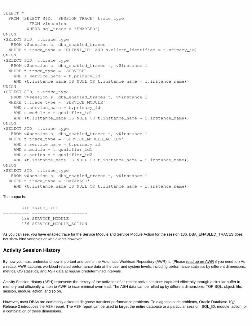
SELECT * FROM (SELECT SID, 'SESSION_TRACE' trace_type FROM v$session WHERE sql_trace = 'ENABLED')UNION(SELECT SID, t.trace_type FROM v$session s, dba_enabled_traces t WHERE t.trace_type = 'CLIENT_ID' AND s.client_identifier = t.primary_id)UNION(SELECT SID, t.trace_type FROM v$session s, dba_enabled_traces t, v$instance i WHERE t.trace_type = 'SERVICE' AND s.service_name = t.primary_id AND (t.instance_name IS NULL OR t.instance_name = i.instance_name))UNION(SELECT SID, t.trace_type FROM v$session s, dba_enabled_traces t, v$instance i WHERE t.trace_type = 'SERVICE_MODULE' AND s.service_name = t.primary_id AND s.module = t.qualifier_id1 AND (t.instance_name IS NULL OR t.instance_name = i.instance_name))UNION(SELECT SID, t.trace_type FROM v$session s, dba_enabled_traces t, v$instance i WHERE t.trace_type = 'SERVICE_MODULE_ACTION' AND s.service_name = t.primary_id AND s.module = t.qualifier_id1 AND s.action = t.qualifier_id2 AND (t.instance_name IS NULL OR t.instance_name = i.instance_name))UNION(SELECT SID, t.trace_type FROM v$session s, dba_enabled_traces t, v$instance i WHERE t.trace_type = 'DATABASE' AND (t.instance_name IS NULL OR t.instance_name = i.instance_name))

The output is:

SID TRACE_TYPE---------- --------------------- 136 SERVICE_MODULE 136 SERVICE_MODULE_ACTION

As you can see, you have enabled trace for the Service Module and Service Module Action for the session 136. DBA_ENABLED_TRACES does not show bind variables or wait events however.

Activity Session History

By now you must understand how important and useful the Automatic Workload Repository (AWR) is. (Please read up on AWR if you need to.) As a recap, AWR captures workload-related performance data at the user and system levels, including performance statistics by different dimensions, metrics, OS statistics, and ASH data at regular predetermined intervals.

Activity Session History (ASH) represents the history of the activities of all recent active sessions captured efficiently through a circular buffer in memory and efficiently written to AWR to incur minimal overhead. The ASH data can be rolled up by different dimensions: TOP SQL, object, file, session, module, action, and so on.

However, most DBAs are commonly asked to diagnose transient performance problems. To diagnose such problems, Oracle Database 10g Release 2 introduces the ASH report. The ASH report can be used to target the entire database or a particular session, SQL_ID, module, action, or a combination of these dimensions.

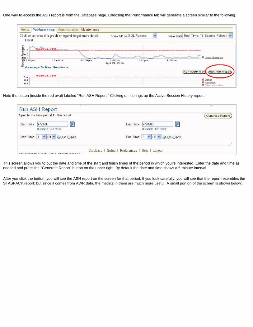
One way to access the ASH report is from the Database page. Choosing the Performance tab will generate a screen similar to the following.

Note the button (inside the red oval) labeled "Run ASH Report." Clicking on it brings up the Active Session History report:

This screen allows you to put the date and time of the start and finish times of the period in which you're interested. Enter the date and time as needed and press the "Generate Report" button on the upper right. By default the date and time shows a 5-minute interval.

After you click the button, you will see the ASH report on the screen for that period. If you look carefully, you will see that the report resembles the STASPACK report; but since it comes from AWR data, the metrics in them are much more useful. A small portion of the screen is shown below:

You can save the report to a file for later viewing by pressing the button "Save to File."

Note the links in the section "ASH Report." Here you can see the different types of available performance-related statistics and metrics in one glance. For instance, you can see Top Events during the period only by clicking on that link. If performance issues come up within the period, this information will help substantially. You can generally identify bottlenecks that caused the transient spikes by looking at skews along the various dimensions listed in the ASH report.

Remember, this report is pulled from data collected by AWR or from in-memory buffers as appropriate; hence, if you want to diagnose a performance issue that occurred earlier, you could simply fire up the ASH report for that period and see any issues that might have surfaced then.

The ASH report can also be run through command line, by running the Oracle supplied SQL script located in $OH/rdbms/admin/ashrpt.sql.

Optimizer Statistics Management

Oracle Database 10g offers several very useful features for managing optimizer statistics, such as one for locking down statistics to prevent subsequent overwriting. These features make the task of collecting and managing optimizer statistics a breeze. And in Oracle Database 10g Release 2, you can do that using Oracle Enterprise Manager.

From the Database home page click on the Administration tab. Go down to the section titled "Statistics Management," where you see the Manage Optimizer Statistics link as shown below.

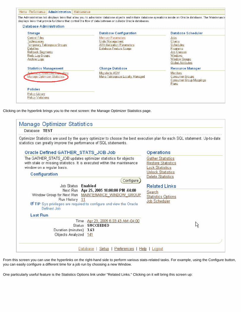
Clicking on the hyperlink brings you to the next screen: the Manage Optimizer Statistics page.

From this screen you can use the hyperlinks on the right-hand side to perform various stats-related tasks. For example, using the Configure button, you can easily configure a different time for a job run by choosing a new Window.

One particularly useful feature is the Statistics Options link under "Related Links." Clicking on it will bring this screen up:

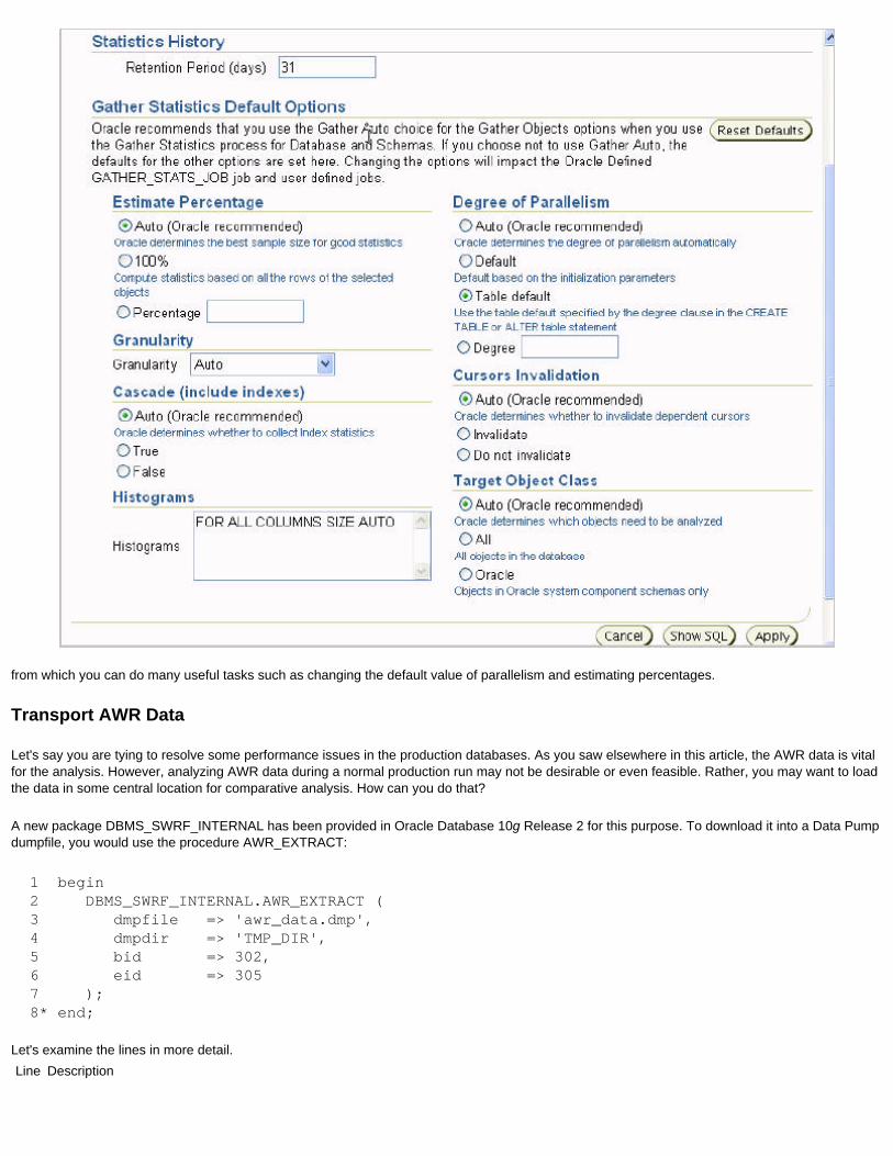
from which you can do many useful tasks such as changing the default value of parallelism and estimating percentages.

Transport AWR Data

Let's say you are tying to resolve some performance issues in the production databases. As you saw elsewhere in this article, the AWR data is vital for the analysis. However, analyzing AWR data during a normal production run may not be desirable or even feasible. Rather, you may want to load the data in some central location for comparative analysis. How can you do that?

A new package DBMS_SWRF_INTERNAL has been provided in Oracle Database 10g Release 2 for this purpose. To download it into a Data Pump dumpfile, you would use the procedure AWR_EXTRACT:

1 begin 2 DBMS_SWRF_INTERNAL.AWR_EXTRACT ( 3 dmpfile => 'awr_data.dmp', 4 dmpdir => 'TMP_DIR', 5 bid => 302, 6 eid => 305 7 ); 8* end;

Let's examine the lines in more detail. Line Description

3 The name of the target file for the data is mentioned here. This is a Data Pump export file. If non filename is given, the default value awrdat.dmp is used.

4 The directory object where the dumpfile is written. In this case, you may have defined a directory TMP_DIR as /tmp.

5 The snapshot ID of the beginning snapshot of the period.

6 The end snapshot ID. Here you are exporting the snapshots between 302 and 305.Now you can take the dumpfile awr_data.dmp to the new location and load it using another procedure in the same package, AWR_LOAD:

1 begin 2 DBMS_SWRF_INTERNAL.AWR_LOAD ( 3 SCHNAME => 'ARUP', 4 dmpfile => 'awr_data', 5 dmpdir => 'TMP_DIR' 6 ); 7* end;

In this code, you are loading the contents of the dumpfile awr_data.dmp into the directory specified by the directory object TMP_DIR. When loading the AWR data, it is not loaded into the SYS schema directly; rather, it's staged in a different schema first. The schema name is given in the parameter SCHNAME, as shown in line 3. After staging, the data is moved into the SYS schema:

1 begin 2 DBMS_SWRF_INTERNAL.MOVE_TO_AWR ( 3 SCHNAME => 'ARUP' 4 ); 5* end;

Here you are moving the AWR data from the schema ARUP to SYS.

Moving AWR to a different database, as I mentioned above, has a lot of benefits and uses. You can analyze the data in a different database without affecting production too much. In addition, you can build a central repository of AWR data collected from multiple databases.

All these loading steps have been placed into a single file awrload.sql located in $ORACLE_HOME/rdbms/bin directory. Similarly, the script awrextr.sql contains all the steps for the extraction process.

While this mechanism for off-loading production AWR data to a secondary database has been externalized, its main intent in Oracle Database 10g Release 2 is to help troubleshoot any problems reported by customers. With this approach, customers can send raw data in the form of AWR dump files , which support staff can then import into their schema to help reproduce and diagnose problems.

Compare Periods Report

Imagine this scenario. You have just been called to an emergency meeting with the business and applications teams. The reason is all too obvious: the database is slow. (Is there ever any other reason?) Anyway, here's the scoop, says the development tech lead: the batch program run last night between 1 a.m. and 3 a.m. was very slow. It always runs at that time for about 30 minutes, but last night it took two hours. And, as if on cue, the business team lead declares: "The company suffered a potential revenue loss."

"Were there any recent changes?", you ask. "Nope, not a thing," is the oh-so-swift reply from the development tech lead. ("Yeah, right," you think.)

Sound familiar? If you have been on the production support hot seat for even a tenth as long as I have, you're nodding in agreement right now. What do you do?

Fortunately, you have Oracle Database 10g Release 2 and fire up the Snapshot or Time Periods comparison in Oracle Enterprise Manager. Using this feature, you can see the metric changes between two time intervals, not just two points in time. For instance, in this case, you could ask to see the snapshot changes between 1 a.m. and 3 a.m. last night and the same for the previous day. If the batch process was running fine the previous day, and not last night, the snapshot changes will give you a big clue.

Here's how it would work: Pull up Oracle Enterprise Manager and go to the Performance tab. Toward the bottom of the page, you will see the section "Additional Monitoring Links." In that group of links, look for "Snapshots." Clicking on that will bring up a screen similar to that shown below.

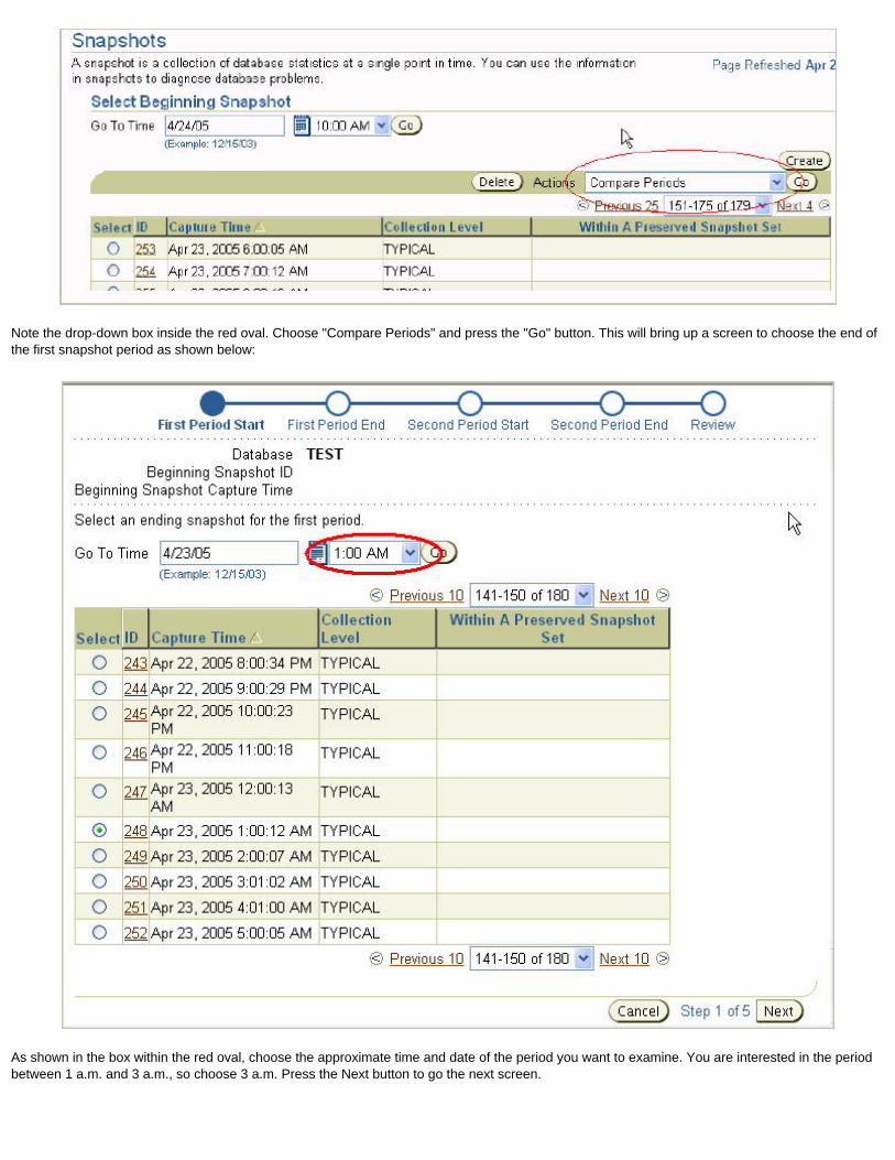
Note the drop-down box inside the red oval. Choose "Compare Periods" and press the "Go" button. This will bring up a screen to choose the end of the first snapshot period as shown below:

As shown in the box within the red oval, choose the approximate time and date of the period you want to examine. You are interested in the period between 1 a.m. and 3 a.m., so choose 3 a.m. Press the Next button to go the next screen.

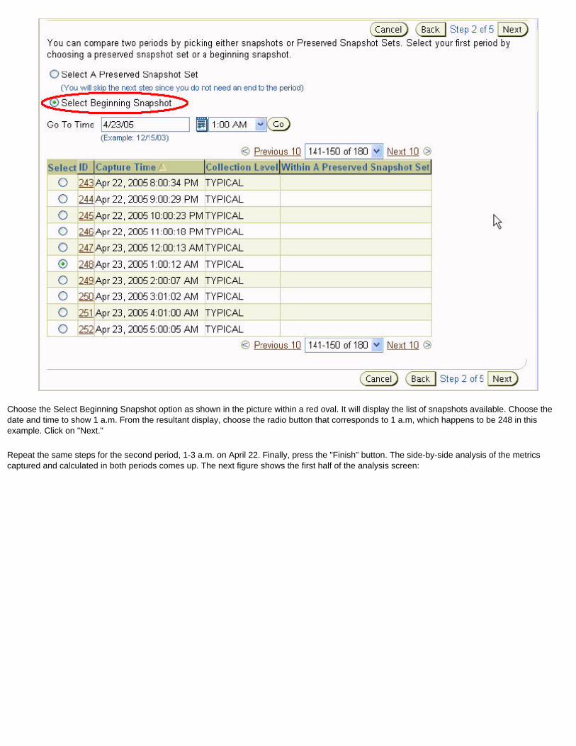
Choose the Select Beginning Snapshot option as shown in the picture within a red oval. It will display the list of snapshots available. Choose the date and time to show 1 a.m. From the resultant display, choose the radio button that corresponds to 1 a.m, which happens to be 248 in this example. Click on "Next."

Repeat the same steps for the second period, 1-3 a.m. on April 22. Finally, press the "Finish" button. The side-by-side analysis of the metrics captured and calculated in both periods comes up. The next figure shows the first half of the analysis screen:

Note how you can see the start and end times of each period. The first column shows different metrics either collected or computed from others; the next columns show how these metrics look in each period. These metrics give you the clues you were looking for to find the discrepancies in performance.

You can make it easier by clicking on the Second Period Rate Per Second column, which sorts its output. Start with the highest to lowest sorting, which shows the worst values at the top. In your example, suppose it says that the physical reads were much higher in the second period. There you go: Now you know why the elapsed time was high. To know what caused the physical reads to go up you cam pull up a report of all the activities and all the metrics, similar to the AWR report—but as a comparative one, not for a specific period. Click on the Report tab and you will see the report similar to the following screen:

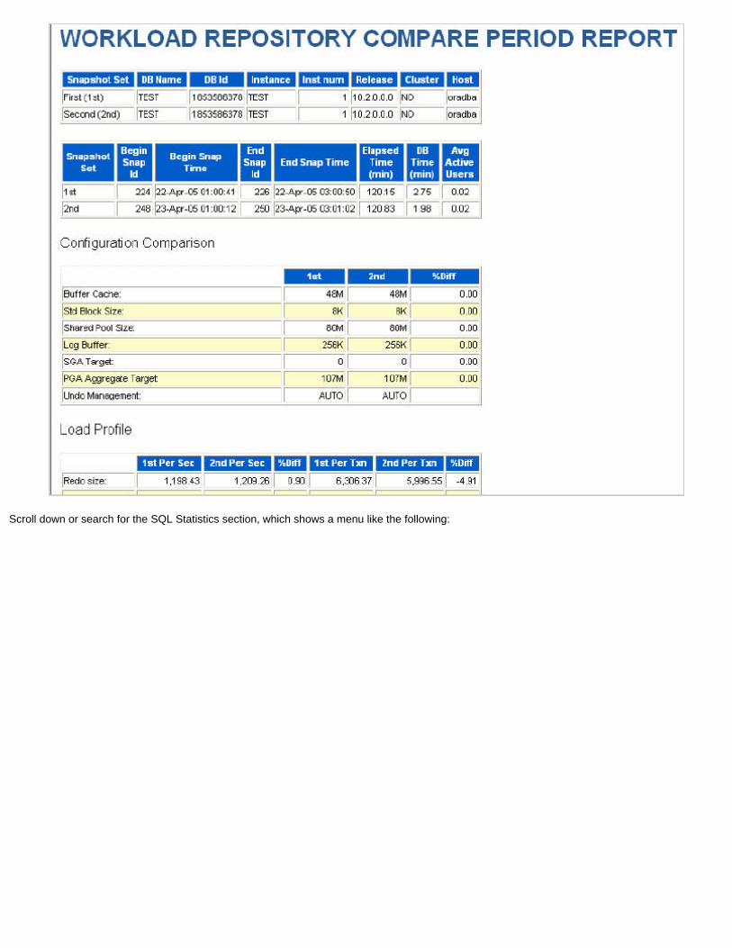
Scroll down or search for the SQL Statistics section, which shows a menu like the following:

Here the SQL statements that caused the physical reads to go up can be explored. Click on the link "Top 10 SQL Comparison by Physical Reads" and it will show you a grid of all the SQL IDs and the corresponding physical reads. You can drill down further by clicking on the SQL ID.

Of course, this is merely an example case. Regardless of the issue, you can easily drill down to find the exact reason performance differed in two periods by doing a comparative analysis. The report also lists all the changes in the database configuration settings for the two time periods being compared. Also, as all the metrics and statistics are appropriately normalized by time for the two time periods being compared, they need not be of the same duration.

In Part 4, I'll cover data warehousing and integration features.

Part 4: Data Warehousing and Integration Features

New features for more efficiently managing materialized views, Query Rewrite, Transportable Tablespace, and table partitions make your data warehouse an even more powerful, and less resource-intensive, asset.

Covered in This Installment: · Partition Change-Tracking Without MV Logs· Query Rewrite with Multiple MVs· Transportable Tablespace From Backup· Quick Partition Split for Partitioned Index-Organized Tables · LONG to LOB Conversion via Online Redef· Online Reorg of a Single Partition· Partition-by-Partition Table Drop

Partition-Change Tracking: No Need for MV Logs

To understand this enhancement, you first have to understand the concept of partition pruning during a materialized view (MV) refresh process.

Suppose the table ACCOUNTS has been partitioned on the column ACC_MGR_ID, with one partition per the value of ACC_MGR_ID. You have

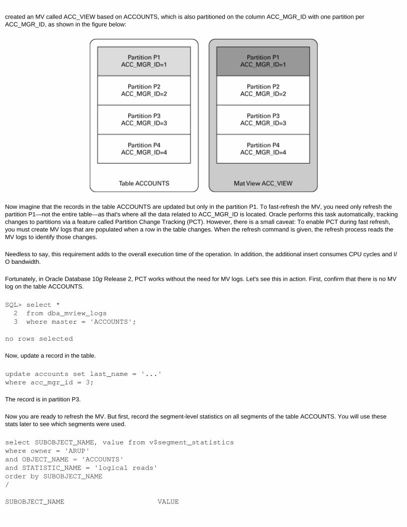
created an MV called ACC_VIEW based on ACCOUNTS, which is also partitioned on the column ACC_MGR_ID with one partition per ACC_MGR_ID, as shown in the figure below:

Now imagine that the records in the table ACCOUNTS are updated but only in the partition P1. To fast-refresh the MV, you need only refresh the partition P1—not the entire table—as that's where all the data related to ACC_MGR_ID is located. Oracle performs this task automatically, tracking changes to partitions via a feature called Partition Change Tracking (PCT). However, there is a small caveat: To enable PCT during fast refresh, you must create MV logs that are populated when a row in the table changes. When the refresh command is given, the refresh process reads the MV logs to identify those changes.

Needless to say, this requirement adds to the overall execution time of the operation. In addition, the additional insert consumes CPU cycles and I/O bandwidth.

Fortunately, in Oracle Database 10g Release 2, PCT works without the need for MV logs. Let's see this in action. First, confirm that there is no MV log on the table ACCOUNTS.

SQL> select * 2 from dba_mview_logs 3 where master = 'ACCOUNTS';

no rows selected

Now, update a record in the table.

update accounts set last_name = '...'where acc_mgr_id = 3;

The record is in partition P3.

Now you are ready to refresh the MV. But first, record the segment-level statistics on all segments of the table ACCOUNTS. You will use these stats later to see which segments were used.

select SUBOBJECT_NAME, value from v$segment_statisticswhere owner = 'ARUP'and OBJECT_NAME = 'ACCOUNTS'and STATISTIC_NAME = 'logical reads'order by SUBOBJECT_NAME/

SUBOBJECT_NAME VALUE

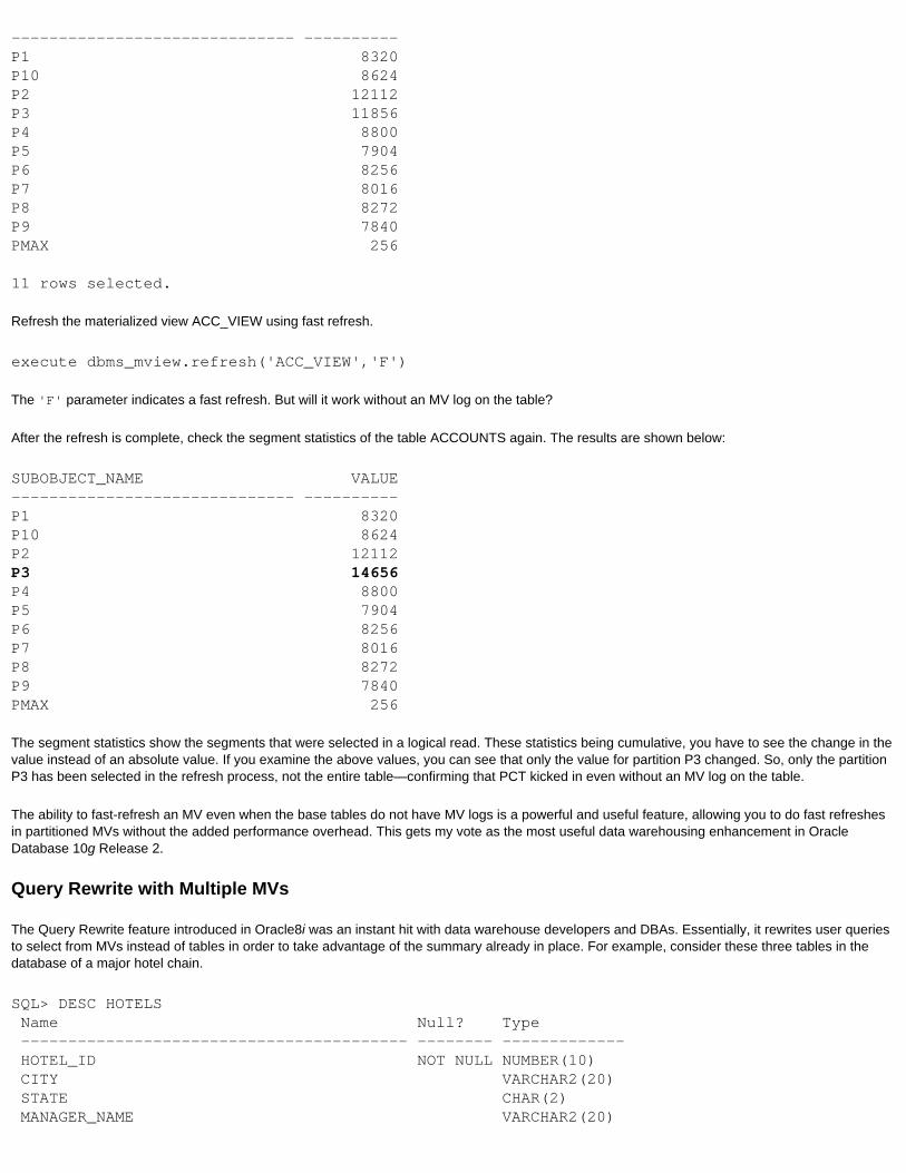
------------------------------ ----------P1 8320P10 8624P2 12112P3 11856P4 8800P5 7904P6 8256P7 8016P8 8272P9 7840PMAX 256

11 rows selected.

Refresh the materialized view ACC_VIEW using fast refresh.

execute dbms_mview.refresh('ACC_VIEW','F')

The 'F' parameter indicates a fast refresh. But will it work without an MV log on the table?

After the refresh is complete, check the segment statistics of the table ACCOUNTS again. The results are shown below:

SUBOBJECT_NAME VALUE------------------------------ ----------P1 8320P10 8624P2 12112P3 14656P4 8800P5 7904P6 8256P7 8016P8 8272P9 7840PMAX 256

The segment statistics show the segments that were selected in a logical read. These statistics being cumulative, you have to see the change in the value instead of an absolute value. If you examine the above values, you can see that only the value for partition P3 changed. So, only the partition P3 has been selected in the refresh process, not the entire table—confirming that PCT kicked in even without an MV log on the table.

The ability to fast-refresh an MV even when the base tables do not have MV logs is a powerful and useful feature, allowing you to do fast refreshes in partitioned MVs without the added performance overhead. This gets my vote as the most useful data warehousing enhancement in Oracle Database 10g Release 2.

Query Rewrite with Multiple MVs

The Query Rewrite feature introduced in Oracle8i was an instant hit with data warehouse developers and DBAs. Essentially, it rewrites user queries to select from MVs instead of tables in order to take advantage of the summary already in place. For example, consider these three tables in the database of a major hotel chain.

SQL> DESC HOTELS Name Null? Type ----------------------------------------- -------- ------------- HOTEL_ID NOT NULL NUMBER(10) CITY VARCHAR2(20) STATE CHAR(2) MANAGER_NAME VARCHAR2(20)

RATE_CLASS CHAR(2)

SQL> DESC RESERVATIONS Name Null? Type ----------------------------------------- -------- ------------- RESV_ID NOT NULL NUMBER(10) HOTEL_ID NUMBER(10) CUST_NAME VARCHAR2(20) START_DATE DATE END_DATE DATE RATE NUMBER(10)

SQL> DESC TRANS Name Null? Type ----------------------------------------- -------- ------------- TRANS_ID NOT NULL NUMBER(10) RESV_ID NOT NULL NUMBER(10) TRANS_DATE DATE ACTUAL_RATE NUMBER(10)

The table HOTELS holds the information on the hotels. When a customer makes a reservation, a record is created in the table RESERVATIONS, which includes the quoted room rate. When the customer checks out of the hotel, the money transactions are recorded in a different table, TRANS.

However, prior to check-out, the hotel may decide to offer a different rate to the customer based on room availability, upgrades, incentives, and do on. Hence the final room rate could differ from the rate quoted during reservation, and may even vary from day to day. To record these fluctuations correctly, the table TRANS holds a row containing rate information for each day of the stay.

To enhance query response times, you may decide to build MVs based on the different queries issued by users, such as

create materialized view mv_hotel_resvrefresh completeenable query rewriteasselect city, resv_id, cust_namefrom hotels h, reservations rwhere r.hotel_id = h.hotel_id;

and

create materialized view mv_actual_salesrefresh completeenable query rewriteasselect resv_id, sum(actual_rate) from trans group by resv_id;

Thus, a query such as

select city, cust_namefrom hotels h, reservations rwhere r.hotel_id = h.hotel_id;

will be rewritten to

select city, cust_namefrom mv_hotel_resv;

provided some parameters are set, such as query_rewrite_enabled = true. You can confirm the MV by running the query and enabling autotrace.

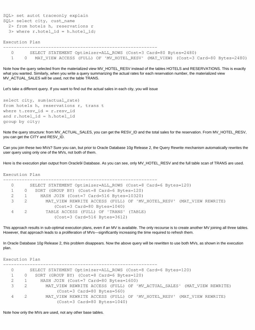
SQL> set autot traceonly explainSQL> select city, cust_name 2> from hotels h, reservations r 3> where r.hotel_id = h.hotel_id;

Execution Plan---------------------------------------------------------- 0 SELECT STATEMENT Optimizer=ALL_ROWS (Cost=3 Card=80 Bytes=2480) 1 0 MAT_VIEW ACCESS (FULL) OF 'MV_HOTEL_RESV' (MAT_VIEW) (Cost=3 Card=80 Bytes=2480)

Note how the query selected from the materialized view MV_HOTEL_RESV instead of the tables HOTELS and RESERVATIONS. This is exactly what you wanted. Similarly, when you write a query summarizing the actual rates for each reservation number, the materialized view MV_ACTUAL_SALES will be used, not the table TRANS.

Let's take a different query. If you want to find out the actual sales in each city, you will issue

select city, sum(actual_rate)from hotels h, reservations r, trans twhere t.resv_id = r.resv_idand r.hotel_id = h.hotel_idgroup by city;

Note the query structure: from MV_ACTUAL_SALES, you can get the RESV_ID and the total sales for the reservation. From MV_HOTEL_RESV, you can get the CITY and RESV_ID.

Can you join these two MVs? Sure you can, but prior to Oracle Database 10g Release 2, the Query Rewrite mechanism automatically rewrites the user query using only one of the MVs, not both of them.

Here is the execution plan output from Oracle9i Database. As you can see, only MV_HOTEL_RESV and the full table scan of TRANS are used.

Execution Plan---------------------------------------------------------- 0 SELECT STATEMENT Optimizer=ALL_ROWS (Cost=8 Card=6 Bytes=120) 1 0 SORT (GROUP BY) (Cost=8 Card=6 Bytes=120) 2 1 HASH JOIN (Cost=7 Card=516 Bytes=10320) 3 2 MAT_VIEW REWRITE ACCESS (FULL) OF 'MV_HOTEL_RESV' (MAT_VIEW REWRITE) (Cost=3 Card=80 Bytes=1040) 4 2 TABLE ACCESS (FULL) OF 'TRANS' (TABLE) (Cost=3 Card=516 Bytes=3612)

This approach results in sub-optimal execution plans, even if an MV is available. The only recourse is to create another MV joining all three tables. However, that approach leads to a proliferation of MVs—significantly increasing the time required to refresh them.

In Oracle Database 10g Release 2, this problem disappears. Now the above query will be rewritten to use both MVs, as shown in the execution plan.

Execution Plan---------------------------------------------------------- 0 SELECT STATEMENT Optimizer=ALL_ROWS (Cost=8 Card=6 Bytes=120) 1 0 SORT (GROUP BY) (Cost=8 Card=6 Bytes=120) 2 1 HASH JOIN (Cost=7 Card=80 Bytes=1600) 3 2 MAT_VIEW REWRITE ACCESS (FULL) OF 'MV_ACTUAL_SALES' (MAT_VIEW REWRITE) (Cost=3 Card=80 Bytes=560) 4 2 MAT_VIEW REWRITE ACCESS (FULL) OF 'MV_HOTEL_RESV' (MAT_VIEW REWRITE) (Cost=3 Card=80 Bytes=1040)

Note how only the MVs are used, not any other base tables.

This enhancement has significant advantages in data warehouse environments because you don't have to create and refresh an MV for each possible query. Instead, you can strategically create a few MVs without too many joins and aggregations and Oracle will use them all to rewrite queries.

Transportable Tablespace from Backup

Transportable tablespaces, introduced in Oracle8i, provided much-needed support for faster data transfer across databases. Using this feature, you can export just the metadata of the tablespace, transfer the data file and the export dump file to the target database host, and import the metadata to "plug" the tablespace into the target database. The data in the tablespace is then instantly available in the target database. This approach solves what was then one of the thorniest issues in data warehousing: moving data across databases quickly and efficiently.

In an OLTP database, however, this condition is almost always impossible, and thus so is transporting tablespaces. If the OLTP database is the data source for the data warehouse, then you may never be able to use Transportable Tablespace to load it.

In Oracle Database 10g Release 2, you can transport a tablespace and plug it in from another source: your backups. For example, if you want to transport the tablespace ACCDATA, you can issue the RMAN command

RMAN> transport tablespace accdata 2> TABLESPACE DESTINATION = '/home/oracle'3> auxiliary destination = '/home/oracle';

which creates an auxiliary instance on the location /home/oracle and restores the files from the backup there. The auxiliary instance name is generated randomly. After creating the instance, the process creates a directory object on the directory and restores the files of the tablespace ACCDATA (the one we are transporting)—all by itself, without a single command from you!

The directory /home/oracle will have all the datafiles of the tablespace ACCDATA, the dump file containing the metadata of the tablespace, and, most important, a script named impscrpt.sql. This script contains all the necessary commands to plug this tablespace into a target tablespace. The tablespace is not transported by the impdp command but rather through the call to the dbms_streams_tablespace_adm.attach_tablespaces package. All the necessary commands can be found in the script.

But what if something goes wrong, you may ask? In that case, making a diagnosis is easy. First, the auxiliary instance creates the alert log file in the location $ORACLE_HOME/rdbms/log, so you can examine the log for potential problems. Second, while giving the RMAN command, you can redirect the commands and the output to a log file by issuing the RMAN command

rman target=/ log=tts.log

which places all the output in the file tts.log. You can then examine the file for the exact cause of the failure.

Finally, the files are restored into the directory TSPITR_<SourceSID>_<AuxSID> in /home/oracle. For instance, if the SID of the main database is ACCT and the SID of the auxiliary instance created by RMAN is KYED, the directory name is TSPITR_ACCT_KYED. The directory also has two other subdirectories: datafile (for datafiles) and onlinelog (for redo logs). Before the new tablespace creation is complete, you can examine the directory to see which files are restored. (These files are deleted at the end of the process.)

DBAs have been waiting for the ability to create a transportable tablespace from RMAN backups for a long time. But bear in mind that you are plugging-in the transported tablespace from backup, not from the online tablespace. So it won't be current.

Quick Partition Split for Partitioned, Index-Organized Tables

Consider this situation: Let's say that you have a partitioned table. The end of the month arrives, but you have forgotten to define a partition for the next month. What are your options now?

Well, your only recourse is to split the maxvalue partition into two parts: the partition for the new month and the new maxvalue partition. However, there is a slight problem when you take that approach for partitioned, index-organized tables. In this case, the physical partition is created first and rows are moved there from the maxvalue partition—thereby consuming I/O as well as CPU cycles.

In Oracle Database 10g Release 2, this process is simplified considerably. As illustrated in the figure below, let's say you have defined partitions up until May and then the PMAX partition has been defined as a catch-all partition. Because there is no specific partition for June, the June data goes into the PMAX partition. The grey-shaded rectangle shows data populated in this segment. Only part of the PMAX partition is filled, so you see only a portion of shading.

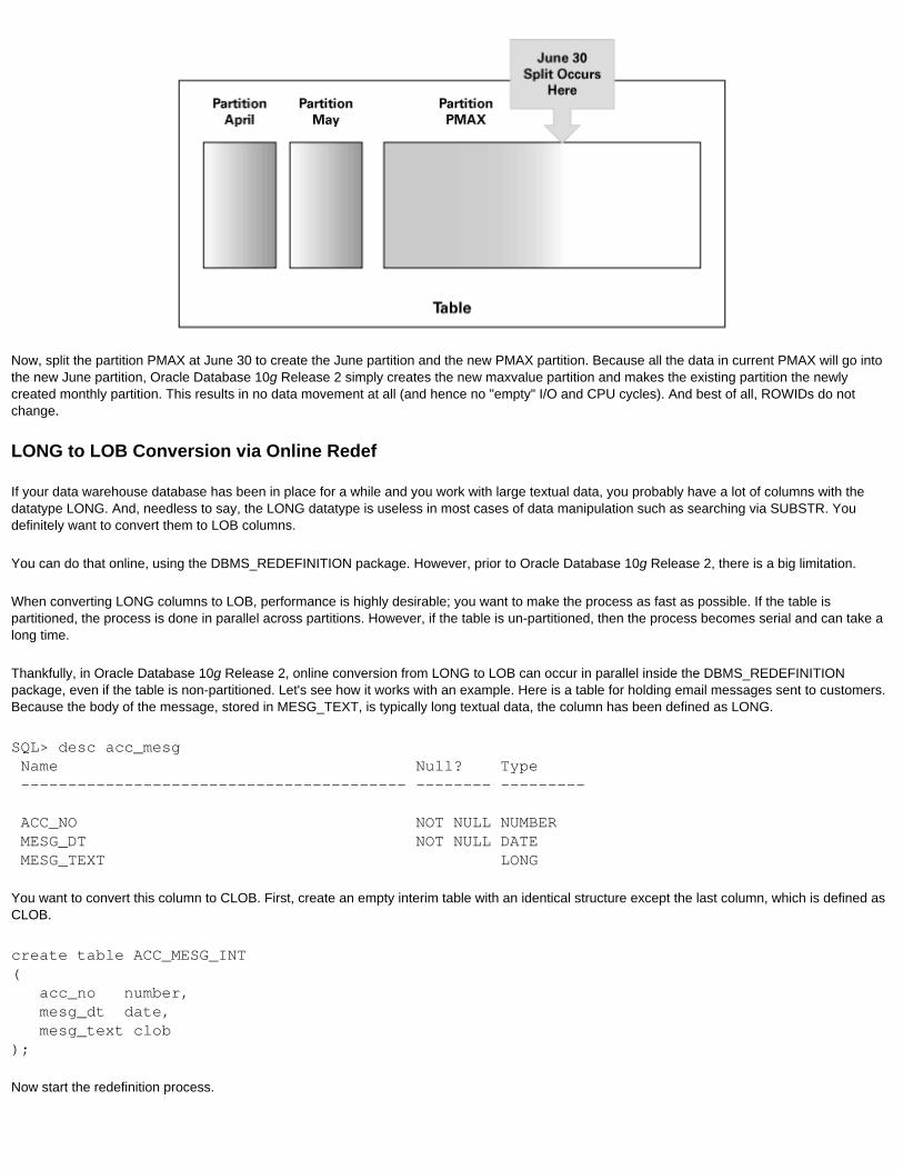
Now, split the partition PMAX at June 30 to create the June partition and the new PMAX partition. Because all the data in current PMAX will go into the new June partition, Oracle Database 10g Release 2 simply creates the new maxvalue partition and makes the existing partition the newly created monthly partition. This results in no data movement at all (and hence no "empty" I/O and CPU cycles). And best of all, ROWIDs do not change.

LONG to LOB Conversion via Online Redef

If your data warehouse database has been in place for a while and you work with large textual data, you probably have a lot of columns with the datatype LONG. And, needless to say, the LONG datatype is useless in most cases of data manipulation such as searching via SUBSTR. You definitely want to convert them to LOB columns.

You can do that online, using the DBMS_REDEFINITION package. However, prior to Oracle Database 10g Release 2, there is a big limitation.

When converting LONG columns to LOB, performance is highly desirable; you want to make the process as fast as possible. If the table is partitioned, the process is done in parallel across partitions. However, if the table is un-partitioned, then the process becomes serial and can take a long time.

Thankfully, in Oracle Database 10g Release 2, online conversion from LONG to LOB can occur in parallel inside the DBMS_REDEFINITION package, even if the table is non-partitioned. Let's see how it works with an example. Here is a table for holding email messages sent to customers. Because the body of the message, stored in MESG_TEXT, is typically long textual data, the column has been defined as LONG.

SQL> desc acc_mesg Name Null? Type ----------------------------------------- -------- ---------

ACC_NO NOT NULL NUMBER MESG_DT NOT NULL DATE MESG_TEXT LONG

You want to convert this column to CLOB. First, create an empty interim table with an identical structure except the last column, which is defined as CLOB.

create table ACC_MESG_INT( acc_no number, mesg_dt date, mesg_text clob);

Now start the redefinition process.

1 begin 2 dbms_redefinition.start_redef_table ( 3 UNAME => 'ARUP', 4 ORIG_TABLE => 'ACC_MESG', 5 INT_TABLE => 'ACC_MESG_INT', 6 COL_MAPPING => 'acc_no acc_no, mesg_dt mesg_dt, to_lob(MESG_TEXT) MESG_TEXT' 7 ); 8* end;

Note line 6, where the columns have been mapped. The first two columns have been left the same but the third column MESG_TEXT has been mapped so that the destination table's column MESG_TEXT is populated by applying the function TO_LOB on the source table's column.

If the table to be redefined is large, you will need to synchronize the data between the source and target tables periodically. This approach makes the final sync-up faster.

begin dbms_redefinition.sync_interim_table( uname => 'ARUP', orig_table => 'ACC_MESG', int_table => 'ACC_MESG_INT' );end;/

You may have to give the above command a few times, depending on the size of the table. Finally, complete the redefinition process with

begin dbms_redefinition.finish_redef_table ( UNAME => 'ARUP', ORIG_TABLE => 'ACC_MESG', INT_TABLE => 'ACC_MESG_INT');end;/

The table ACC_MESG has changed:

SQL> desc acc_mesg Name Null? Type ----------------------------------------- -------- ---------

ACC_NO NOT NULL NUMBER MESG_DT NOT NULL DATE MESG_TEXT

Note the column MESG_TEXT is now CLOB, instead of LONG.

This feature is very useful for converting incorrectly defined or legacy leftover data structures into more manageable datatypes.

Online Reorg of a Single Partition

Suppose you have a table TRANS that contains history of transactions. This table is partitioned on the TRANS_DATE, with each quarter as a partition. During the normal course of business, the most recent partitions are updated frequently. After a quarter is complete, there may not be much activity on that partition and it can be moved to a different location. However, the move itself will require a lock on the table, denying public access to the partition. How can you move the partition with no impact on its availability?

In Oracle Database 10g Release 2, you can use online redefinition on a single partition. You can perform this task just as you would for the entire table—using the DBMS_REDEFINITION package—but the underlying mechanism is different. Whereas regular tables are redefined by creating a

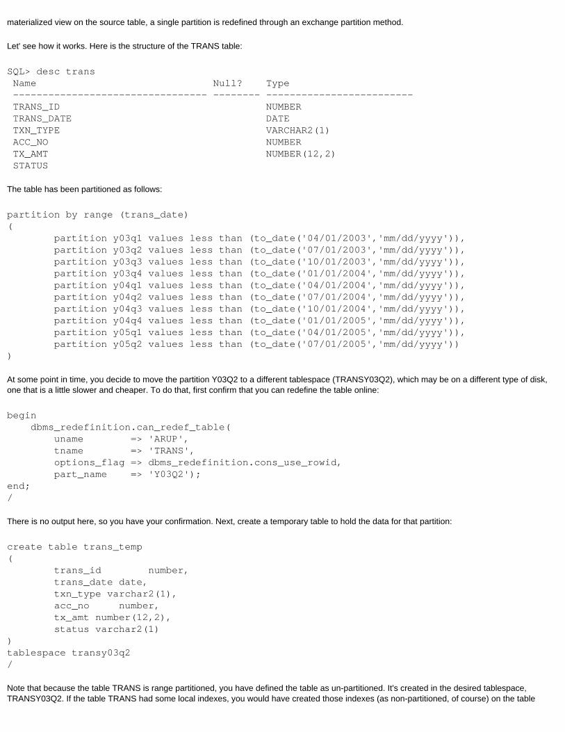
materialized view on the source table, a single partition is redefined through an exchange partition method.

Let' see how it works. Here is the structure of the TRANS table:

SQL> desc trans Name Null? Type --------------------------------- -------- ------------------------- TRANS_ID NUMBER TRANS_DATE DATE TXN_TYPE VARCHAR2(1) ACC_NO NUMBER TX_AMT NUMBER(12,2) STATUS

The table has been partitioned as follows:

partition by range (trans_date)( partition y03q1 values less than (to_date('04/01/2003','mm/dd/yyyy')), partition y03q2 values less than (to_date('07/01/2003','mm/dd/yyyy')), partition y03q3 values less than (to_date('10/01/2003','mm/dd/yyyy')), partition y03q4 values less than (to_date('01/01/2004','mm/dd/yyyy')), partition y04q1 values less than (to_date('04/01/2004','mm/dd/yyyy')), partition y04q2 values less than (to_date('07/01/2004','mm/dd/yyyy')), partition y04q3 values less than (to_date('10/01/2004','mm/dd/yyyy')), partition y04q4 values less than (to_date('01/01/2005','mm/dd/yyyy')), partition y05q1 values less than (to_date('04/01/2005','mm/dd/yyyy')), partition y05q2 values less than (to_date('07/01/2005','mm/dd/yyyy')))

At some point in time, you decide to move the partition Y03Q2 to a different tablespace (TRANSY03Q2), which may be on a different type of disk, one that is a little slower and cheaper. To do that, first confirm that you can redefine the table online:

begin dbms_redefinition.can_redef_table( uname => 'ARUP', tname => 'TRANS', options_flag => dbms_redefinition.cons_use_rowid, part_name => 'Y03Q2'); end; /

There is no output here, so you have your confirmation. Next, create a temporary table to hold the data for that partition:

create table trans_temp( trans_id number, trans_date date, txn_type varchar2(1), acc_no number, tx_amt number(12,2), status varchar2(1))tablespace transy03q2/

Note that because the table TRANS is range partitioned, you have defined the table as un-partitioned. It's created in the desired tablespace, TRANSY03Q2. If the table TRANS had some local indexes, you would have created those indexes (as non-partitioned, of course) on the table

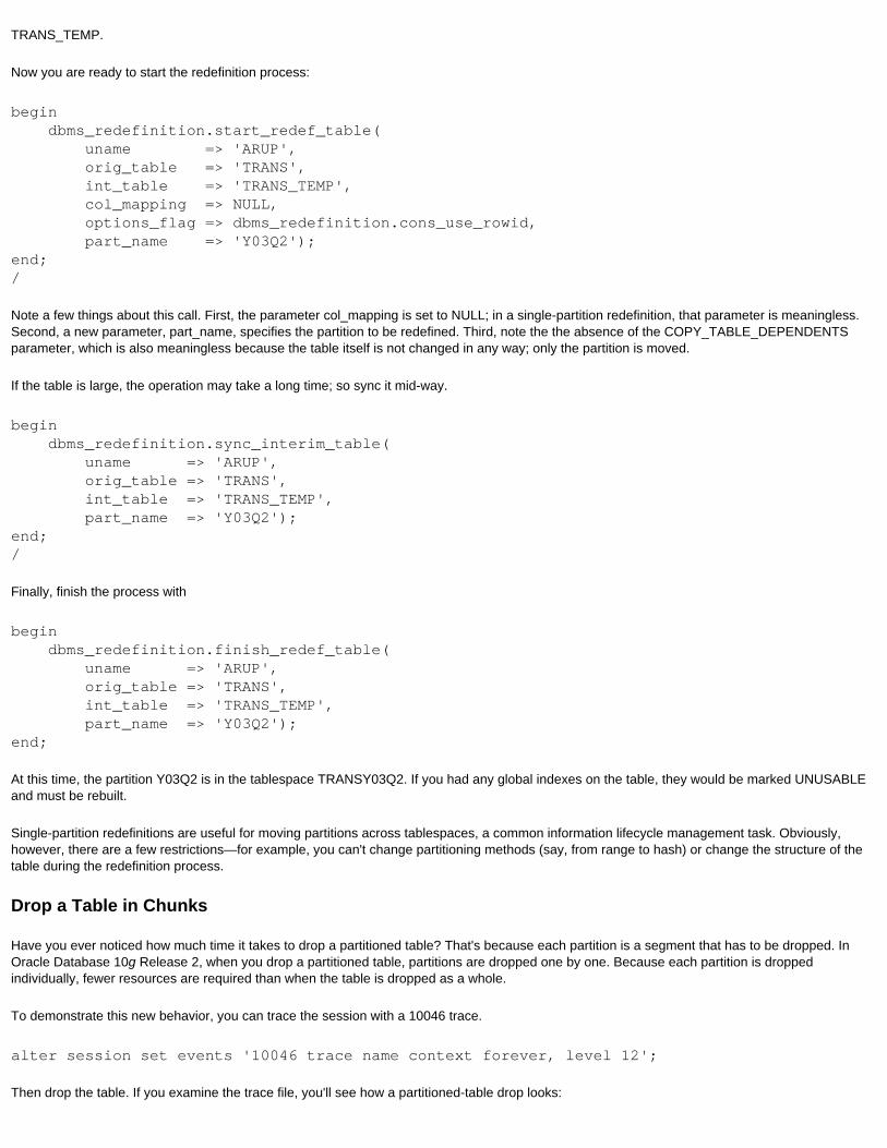
TRANS_TEMP.

Now you are ready to start the redefinition process:

begin dbms_redefinition.start_redef_table( uname => 'ARUP', orig_table => 'TRANS', int_table => 'TRANS_TEMP', col_mapping => NULL, options_flag => dbms_redefinition.cons_use_rowid, part_name => 'Y03Q2'); end;/

Note a few things about this call. First, the parameter col_mapping is set to NULL; in a single-partition redefinition, that parameter is meaningless. Second, a new parameter, part_name, specifies the partition to be redefined. Third, note the the absence of the COPY_TABLE_DEPENDENTS parameter, which is also meaningless because the table itself is not changed in any way; only the partition is moved.

If the table is large, the operation may take a long time; so sync it mid-way.

begin dbms_redefinition.sync_interim_table( uname => 'ARUP', orig_table => 'TRANS', int_table => 'TRANS_TEMP', part_name => 'Y03Q2'); end;/

Finally, finish the process with

begin dbms_redefinition.finish_redef_table( uname => 'ARUP', orig_table => 'TRANS', int_table => 'TRANS_TEMP', part_name => 'Y03Q2'); end;

At this time, the partition Y03Q2 is in the tablespace TRANSY03Q2. If you had any global indexes on the table, they would be marked UNUSABLE and must be rebuilt.

Single-partition redefinitions are useful for moving partitions across tablespaces, a common information lifecycle management task. Obviously, however, there are a few restrictions—for example, you can't change partitioning methods (say, from range to hash) or change the structure of the table during the redefinition process.

Drop a Table in Chunks

Have you ever noticed how much time it takes to drop a partitioned table? That's because each partition is a segment that has to be dropped. In Oracle Database 10g Release 2, when you drop a partitioned table, partitions are dropped one by one. Because each partition is dropped individually, fewer resources are required than when the table is dropped as a whole.

To demonstrate this new behavior, you can trace the session with a 10046 trace.

alter session set events '10046 trace name context forever, level 12';

Then drop the table. If you examine the trace file, you'll see how a partitioned-table drop looks:

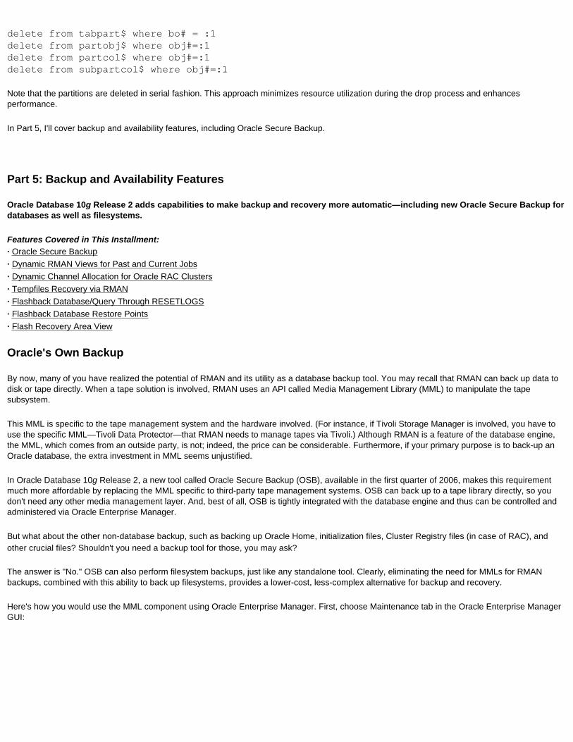
delete from tabpart$ where bo# = :1delete from partobj$ where obj#=:1delete from partcol$ where obj#=:1delete from subpartcol$ where obj#=:1

Note that the partitions are deleted in serial fashion. This approach minimizes resource utilization during the drop process and enhances performance.

In Part 5, I'll cover backup and availability features, including Oracle Secure Backup.

Part 5: Backup and Availability Features

Oracle Database 10g Release 2 adds capabilities to make backup and recovery more automatic—including new Oracle Secure Backup for databases as well as filesystems.

Features Covered in This Installment: · Oracle Secure Backup· Dynamic RMAN Views for Past and Current Jobs· Dynamic Channel Allocation for Oracle RAC Clusters· Tempfiles Recovery via RMAN· Flashback Database/Query Through RESETLOGS· Flashback Database Restore Points· Flash Recovery Area View

Oracle's Own Backup

By now, many of you have realized the potential of RMAN and its utility as a database backup tool. You may recall that RMAN can back up data to disk or tape directly. When a tape solution is involved, RMAN uses an API called Media Management Library (MML) to manipulate the tape subsystem.

This MML is specific to the tape management system and the hardware involved. (For instance, if Tivoli Storage Manager is involved, you have to use the specific MML—Tivoli Data Protector—that RMAN needs to manage tapes via Tivoli.) Although RMAN is a feature of the database engine, the MML, which comes from an outside party, is not; indeed, the price can be considerable. Furthermore, if your primary purpose is to back-up an Oracle database, the extra investment in MML seems unjustified.

In Oracle Database 10g Release 2, a new tool called Oracle Secure Backup (OSB), available in the first quarter of 2006, makes this requirement much more affordable by replacing the MML specific to third-party tape management systems. OSB can back up to a tape library directly, so you don't need any other media management layer. And, best of all, OSB is tightly integrated with the database engine and thus can be controlled and administered via Oracle Enterprise Manager.

But what about the other non-database backup, such as backing up Oracle Home, initialization files, Cluster Registry files (in case of RAC), and other crucial files? Shouldn't you need a backup tool for those, you may ask?

The answer is "No." OSB can also perform filesystem backups, just like any standalone tool. Clearly, eliminating the need for MMLs for RMAN backups, combined with this ability to back up filesystems, provides a lower-cost, less-complex alternative for backup and recovery.

Here's how you would use the MML component using Oracle Enterprise Manager. First, choose Maintenance tab in the Oracle Enterprise Manager GUI:

From the above menu, select the hyperlink titled "Configure Backup Settings," which brings up a screen such as the following:

On this screen, note the "Tape Settings" section, which is where you would configure the Oracle Backup tool.

The Oracle Backup Administrative software can run on a separate host where the software is managed with agents running on the database servers. In this case, the Administrative host is installed and running on host proliback.proligence.com and the Oracle Backup tool has been installed in /bin/obt directory.

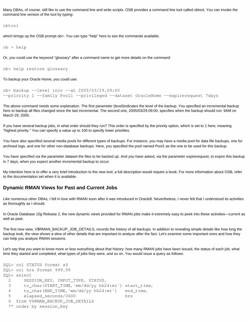
Many DBAs, of course, still like to use the command line and write scripts. OSB provides a command line tool called obtool. You can invoke the command line version of the tool by typing:

obtool

which brings up the OSB prompt ob>. You can type "help" here to see the commands available.

ob > help

Or, you could use the keyword "glossary" after a command name to get more details on the command:

ob> help restore glossary

To backup your Oracle Home, you could use:

ob> backup --level incr --at 2005/03/29.09:00 --priority 1 --family Pool1 --privileged --dataset OracleHome --expirerequest 7days

The above command needs some explanation. The first parameter (level)indicates the level of the backup. You specified an incremental backup here to backup all files changed since the last incremental. The second one, 2005/03/29.09:00, specifies when the backup should run: 9AM on March 29, 2005.

If you have several backup jobs, in what order should they run? This order is specified by the priority option, which is set to 1 here, meaning "highest priority." You can specify a value up to 100 to specify lower priorities.

You have also specified several media pools for different types of backups. For instance, you may have a media pool for data file backups, one for archived logs, and one for other non-database backups. Here, you specified the pool named Pool1 as the one to be used for this backup.

You have specified via the parameter dataset the files to be backed up. And you have asked, via the parameter expirerequest, to expire this backup in 7 days, when you expect another incremental backup to occur.

My intention here is to offer a very brief introduction to the new tool; a full description would require a book. For more information about OSB, refer to the documentation set when it is available.

Dynamic RMAN Views for Past and Current Jobs

Like numerous other DBAs, I fell in love with RMAN soon after it was introduced in Oracle8. Nevertheless, I never felt that I understood its activities as thoroughly as I should.

In Oracle Database 10g Release 2, the new dynamic views provided for RMAN jobs make it extremely easy to peek into these activities—current as well as past.

The first new view, V$RMAN_BACKUP_JOB_DETAILS, records the history of all backups. In addition to revealing simple details like how long the backup took, the view shows a slew of other details that are important to analyze after the fact. Let's examine some important ones and how they can help you analyze RMAN sessions.

Let's say that you want to know more or less everything about that history: how many RMAN jobs have been issued, the status of each job, what time they started and completed, what types of jobs they were, and so on. You would issue a query as follows:

SQL> col STATUS format a9SQL> col hrs format 999.99SQL> select 2 SESSION_KEY, INPUT_TYPE, STATUS, 3 to_char(START_TIME,'mm/dd/yy hh24:mi') start_time, 4 to_char(END_TIME,'mm/dd/yy hh24:mi') end_time, 5 elapsed_seconds/3600 hrs 6 from V$RMAN_BACKUP_JOB_DETAILS 7* order by session_key

The output may resemble the one shown below:

SESSION_KEY INPUT_TYPE STATUS START_TIME END_TIME HRS----------- ------------- -------- -------------- ------------- ------- 1 DATAFILE FULL COMPLETED 03/25/05 00:48 03/25/05 00:48 .00 4 DB FULL COMPLETED 03/27/05 02:09 03/27/05 02:11 .04 7 DB FULL FAILED 03/27/05 02:18 03/27/05 02:24 .10

The SESSION KEY column is the key to the other views showing other relevant information. (More on that in a moment.) The columns START_TIME and END_TIME are fairly intuitive. The column ELAPSED_SECONDS shows the elapsed time in seconds, which I have converted to hour format for easy reading. The STATUS column shows the status of the RMAN jobs. When the job is in progress, the status column shows RUNNING.

Another important piece of information recorded is the rate of the backup produced and how fast data was read and written by the process. This information helps you diagnose any slowness in the RMAN jobs.

SQL> col ins format a10SQL> col outs format a10SQL> select SESSION_KEY, 2 OPTIMIZED, 3 COMPRESSION_RATIO, 4 INPUT_BYTES_PER_SEC_DISPLAY ins, 5 OUTPUT_BYTES_PER_SEC_DISPLAY outs, 6 TIME_TAKEN_DISPLAY 7 from V$RMAN_BACKUP_JOB_DETAILS 8 order by session_key;

SESSION_KEY OPT COMPRESSION_RATIO INS OUTS TIME_TAKEN----------- --- ----------------- ---------- ---------- ---------- 1 NO 2.23776224 3.33M 1.49M 00:00:06 4 NO 1.31065794 6.92M 5.28M 00:02:16 7 NO 1.32363058 3.68M 2.78M 00:06:00

Note how the time is displayed in a human-readable format: in hours:minutes:seconds format. The columns INS and OUTS display the data input or output per seconds, in the easier-to-read format such as M for megabytes. In the above example, you can see that the job marked by session key 4 saw a read rate of 6.92MB/s and 5.2MB/s. You can now examine the output for several RMAN executions and look for a pattern emerging from them. This pattern analysis will help you identify any potential bottlenecks revealed through variations.

The backup information can also be filtered by backup type. The new view V$RMAN_BACKUP_JOB_DETAILS provides the type of backups RMAN performs and how the output can be organized.

SQL> select * from V$RMAN_BACKUP_TYPE;

WEIGHT INPUT_TYPE---------- ------------- 1 BACKUPSET 2 SPFILE 3 CONTROLFILE 4 ARCHIVELOG 5 DATAFILE INCR 6 DATAFILE FULL 7 DB INCR 8 RECVR AREA 9 DB FULL

The object type weight determines how the records in the view are ordered.

Another very useful view is the RMAN output. Say you have run an RMAN job via a shell script but something failed. Sure, you have an output file

that records the RMAN output, but unfortunately, you have lost it. What can you do? Fortunately, the new view V$RMAN_OUTPUT records the output from the RMAN jobs viewing later. This view is useful for scripted RMAN jobs as well as ad-hoc jobs.

SQL> select output 2 from v$rman_output 3 where session_key = 4 4 order by recid;

OUTPUT----------------------------------------------------------------------

connected to target database: TEST (DBID=1849323268)

Starting backup at 27-MAR-05using target database controlfile instead of recovery catalogallocated channel: ORA_DISK_1channel ORA_DISK_1: sid=201 devtype=DISKchannel ORA_DISK_1: starting full datafile backupsetchannel ORA_DISK_1: specifying datafile(s) in backupsetinput datafile fno=00001 name=/u01/app/oracle/oradata/TEST/system01.dbfinput datafile fno=00003 name=/u01/app/oracle/oradata/TEST/sysaux01.dbfinput datafile fno=00002 name=/u01/app/oracle/oradata/TEST/undotbs01.dbfinput datafile fno=00004 name=/u01/app/oracle/oradata/TEST/users01.dbfinput datafile fno=00005 name=/u01/app/oracle/oradata/TEST/accdata01.dbfchannel ORA_DISK_1: starting piece 1 at 27-MAR-05channel ORA_DISK_1: finished piece 1 at 27-MAR-05piece handle=/u01/app/oracle/product/10.2.0/db_1/dbs/07ggc7qr_1_1 comment=NONEchannel ORA_DISK_1: backup set complete, elapsed time: 00:01:46channel ORA_DISK_1: starting full datafile backupsetchannel ORA_DISK_1: specifying datafile(s) in backupsetincluding current controlfile in backupsetchannel ORA_DISK_1: starting piece 1 at 27-MAR-05channel ORA_DISK_1: finished piece 1 at 27-MAR-05piece handle=/u01/app/oracle/product/10.2.0/db_1/dbs/08ggc7u6_1_1 comment=NONEchannel ORA_DISK_1: backup set complete, elapsed time: 00:00:03Finished backup at 27-MAR-05

As you can see, the entire output from the RMAN job is captured here. This is an in-memory view and is cleared when the instance is shut down. If you want the RMAN output to be persistent, the rows can be copied to a permanent table. The column SESSION_KEY shows the records associated with the RMAN jobs shown in the view V$RMAN_BACKUP_JOB_DETAILS. Now you will never lose the output from the RMAN job again.

Via Oracle Enterprise Manager you can utilize the new views to create a new backup report. This report provides an instantaneous overview of backup operations that have been made in your enterprise. You can filter the data by backup type and status.

Dynamic Channel Allocation for Oracle RAC Clusters

In an Oracle RAC environment, of course, there is more than one instance of a database running on more than one host. However, when you invoke RMAN in such an environment you have to connect to only one instance (using TARGET=/), making one node do all the work while the other node remains relatively idle.

Prior to Oracle Database 10g Release 2, one way to make both nodes do the work is to create multiple channels connecting to multiple instances. An example of the associated RMAN command is shown here:

allocate channel = c1 type sbt_tape connect = 'rman/rmanpass@inst1';allocate channel = c2 type sbt_tape connect = 'rman/rmanpass@inst2';

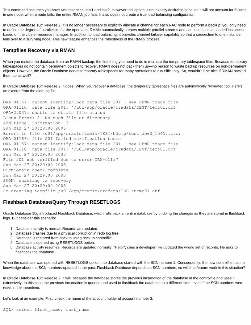
This command assumes you have two instances, inst1 and inst2. However this option is not exactly desirable because it will not account for failures in one node; when a node fails, the entire RMAN job fails. It also does not create a true load-balancing configuration.

In Oracle Database 10g Release 2, it is no longer necessary to explicitly allocate a channel for each RAC node to perform a backup; you only need to define the degree of parallelism for the operation. RMAN automatically creates multiple parallel streams and connects to least loaded instances based on the cluster resource manager. In addition to load balancing, it provides channel failover capability so that a connection to one instance fails over to a surviving node. This new feature enhances the robustness of the RMAN process.

Tempfiles Recovery via RMAN

When you restore the database from an RMAN backup, the first thing you need to do is recreate the temporary tablespace files. Because temporary tablespaces do not contain permanent objects to recover, RMAN does not back them up—no reason to waste backup resources on non-permanent objects. However, the Oracle Database needs temporary tablespaces for many operations to run efficiently. So, wouldn't it be nice if RMAN backed them up as well?

In Oracle Database 10g Release 2, it does. When you recover a database, the temporary tablespace files are automatically recreated too. Here's an excerpt from the alert log file:

ORA-01157: cannot identify/lock data file 201 - see DBWR trace fileORA-01110: data file 201: '/u01/app/oracle/oradata/TEST/temp01.dbf'ORA-27037: unable to obtain file statusLinux Error: 2: No such file or directoryAdditional information: 3Sun Mar 27 20:29:00 2005Errors in file /u01/app/oracle/admin/TEST/bdump/test_dbw0_15457.trc:ORA-01186: file 201 failed verification testsORA-01157: cannot identify/lock data file 201 - see DBWR trace fileORA-01110: data file 201: '/u01/app/oracle/oradata/TEST/temp01.dbf'Sun Mar 27 20:29:00 2005File 201 not verified due to error ORA-01157Sun Mar 27 20:29:00 2005Dictionary check completeSun Mar 27 20:29:00 2005SMON: enabling tx recoverySun Mar 27 20:29:00 2005Re-creating tempfile /u01/app/oracle/oradata/TEST/temp01.dbf

Flashback Database/Query Through RESETLOGS

Oracle Database 10g introduced Flashback Database, which rolls back an entire database by undoing the changes as they are stored in flashback logs. But consider this scenario:

1. Database activity is normal. Records are updated.2. Database crashes due to a physical corruption in redo log files.3. Database is restored from backup using backup controlfile.4. Database is opened using RESETLOGS option.5. Database activity resumes. Records are updated normally. "Help!", cries a developer! He updated the wrong set of records. He asks to

flashback the database.

When the database was opened with RESETLOGS option, the database started with the SCN number 1. Consequently, the new controlfile has no knowledge about the SCN numbers updated in the past. Flashback Database depends on SCN numbers, so will that feature work in this situation?

In Oracle Database 10g Release 2, it will, because the database stores the previous incarnation of the database in the controlfile and uses it extensively. In this case the previous incarnation is queried and used to flashback the database to a different time, even if the SCN numbers were reset in the meantime.

Let's look at an example. First, check the name of the account holder of account number 3.

SQL> select first_name, last_name

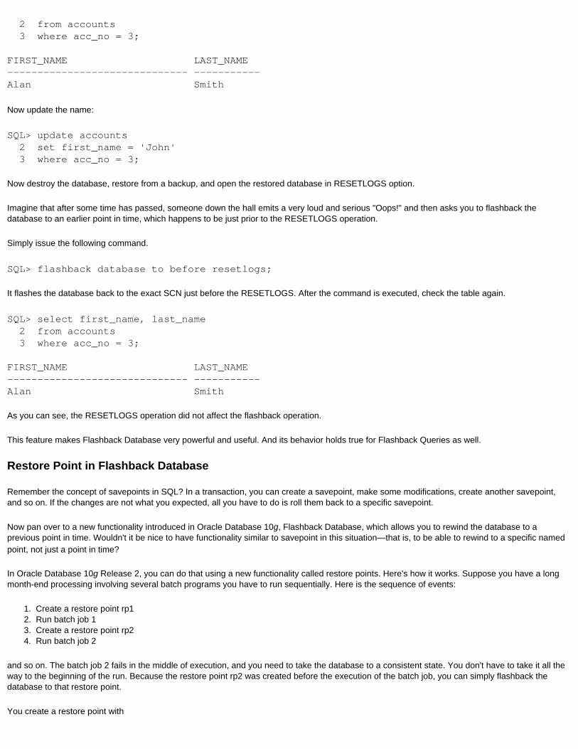
2 from accounts 3 where acc_no = 3;

FIRST_NAME LAST_NAME------------------------------ -----------Alan Smith

Now update the name:

SQL> update accounts 2 set first_name = 'John' 3 where acc_no = 3;

Now destroy the database, restore from a backup, and open the restored database in RESETLOGS option.

Imagine that after some time has passed, someone down the hall emits a very loud and serious "Oops!" and then asks you to flashback the database to an earlier point in time, which happens to be just prior to the RESETLOGS operation.

Simply issue the following command.

SQL> flashback database to before resetlogs;

It flashes the database back to the exact SCN just before the RESETLOGS. After the command is executed, check the table again.

SQL> select first_name, last_name 2 from accounts 3 where acc_no = 3;

FIRST_NAME LAST_NAME------------------------------ -----------Alan Smith

As you can see, the RESETLOGS operation did not affect the flashback operation.

This feature makes Flashback Database very powerful and useful. And its behavior holds true for Flashback Queries as well.

Restore Point in Flashback Database

Remember the concept of savepoints in SQL? In a transaction, you can create a savepoint, make some modifications, create another savepoint, and so on. If the changes are not what you expected, all you have to do is roll them back to a specific savepoint.

Now pan over to a new functionality introduced in Oracle Database 10g, Flashback Database, which allows you to rewind the database to a previous point in time. Wouldn't it be nice to have functionality similar to savepoint in this situation—that is, to be able to rewind to a specific named point, not just a point in time?

In Oracle Database 10g Release 2, you can do that using a new functionality called restore points. Here's how it works. Suppose you have a long month-end processing involving several batch programs you have to run sequentially. Here is the sequence of events:

1. Create a restore point rp12. Run batch job 13. Create a restore point rp24. Run batch job 2

and so on. The batch job 2 fails in the middle of execution, and you need to take the database to a consistent state. You don't have to take it all the way to the beginning of the run. Because the restore point rp2 was created before the execution of the batch job, you can simply flashback the database to that restore point.

You create a restore point with

create restore point before_monthend_200503;

Restore point BEFORE_MONTHEND_200503 is now created based on the current database time and SCN. If you want to ensure that the database can be flashed back to a particular restore point, you can specify a guarantee by creating guaranteed restore points as shown below:

create restore point before_monthend_200503guarantee flashback database;

You can confirm the existence of this restore point by SELECTing from a dynamic performance view V$RESTORE_POINT:

SQL> select * from v$restore_point;

SCN DATABASE_INCARNATION# GUA STORAGE_SIZE---------- --------------------- --- ------------TIME---------------------------------------------------NAME---------------------------------------------------

1429811 1 YES 819200027-MAR-05 05.18.39.000000000 PMBEFORE_MONTHEND_200503

Later when you want to flashback the database to that restore point, you could simply issue:

flashback database to restore point before_monthend_200503;

If you examine the alert log, it will show a line similar to:

Media Recovery Applied UNTIL CHANGE 1429814

Restore points—especially guaranteed restore points—are quite useful in many database-related tasks. A good example is QA databases, where you may want to establish a restore point, run some tests, and flashback to the restore point to make the database look as if nothing happened. Then you can perform another round of testing and again restore it to the restore point.

Peek into the Flash Recovery Area

You may have configured Flash Recovery Area to back up different types of files. But how do you know what types of backups are available there?

A new view, V$FLASH_RECOVERY_AREA_USAGE, shows what's available in the flashback area.

SQL> select * from V$FLASH_RECOVERY_AREA_USAGE;

FILE_TYPE PERCENT_SPACE_USED PERCENT_SPACE_RECLAIMABLE NUMBER_OF_FILES ------------ ------------------ ------------------------- --------------- CONTROLFILE 0 0 0 ONLINELOG 0 0 0 ARCHIVELOG .02 .02 1 BACKUPPIECE 68.98 1.02 10 IMAGECOPY 0 0 0 FLASHBACKLOG .95 0 3

Using this view you can immediately see what kind of files are available in the Flash Recovery Area. It only shows a percentage however, so how do you determine actual values? Simply query the view $RECOVERY_FILE_DEST.

SQL> select * from V$RECOVERY_FILE_DEST;

NAME----------------------------------------------------------SPACE_LIMIT SPACE_USED SPACE_RECLAIMABLE NUMBER_OF_FILES----------- ---------- ----------------- ---------------/home/oracle 2147483648 1502122496 22201856 14

This query shows that the total size of the recovery area is 16384000. Flashback logs occupy 0.95% of the column SPACE_LIMIT as shown in the previous query, so you can calculate the actual size of the space occupied. It also shows you how much space can be reclaimed from the different types of backups in the Flash Recovery Area. For instance, you can reclaim 1.02% of the space occupied by backup pieces, perhaps due to obsolete backups. Using this view you can make intelligent predictions about Flash Recovery Area usage and sizing.

Oracle Enterprise Manager utilizes the new V$RECOVERY_FILE_DEST view by adding a pie chart to the Recovery Settings page that shows the breakdown of files in the Flash Recovery Area:

One of the unique aspects of a DBA's job—especially a production support DBA's job—is the ability to successfully, reliably, and efficiently backup and restore. In Oracle Database 10g Release 2, enhancements in this area make the DBA's job much easier and more reliable.

Back to Series Index