Option Valuation under Stochastic Volatility With ... · In this chapter we introduce a transform-based approach to solving the option valuation PDE that we ... a pure investor model

Option Valuation under Stochastic VolatilityWith Mathematica Code

Copyright µ 2000 by Alan L. Lewis

All rights reserved. Except for the quotation of short passages for the purposesof criticism and review, no part of this publication may be reproduced, stored ina retrieval system, or transmitted, in any form or by any means, electronic,mechanical, photocopying, recording or otherwise, without the prior permissionof the publisher.

Reasonable efforts have been made to publish reliable data and information, butthe author and the publisher cannot assume responsibility for the validity of allmaterials or the consequences of their use. All information, including formulas,documentation, computer algorithms, and computer code are provided with nowarranty of any kind, express or implied. Neither the author nor the publisheraccept any responsibility or liability for the consequences of using them, anddo not claim that they serve any particular purpose or are free from errors.

Published by: Finance Press, Newport Beach, California, USACover design by: Brian Burton Design

For the latest available updates and corrections to this book and publishercontact information, visit the Internet sites:http:// www.financepress.com or http://members.home.net/financepress

Trademark notice: Mathematica is a trademark of Wolfram Research, Inc.,which is not associated with the author or publisher of this book.

International Standard Book Number 0-9676372-0-1Library of Congress Card Number: 99-91935

Printed in the United States of AmericaPrinted on acid-free paper

The Fundamental Transform 35

2 The Fundamental Transform

In this chapter we introduce a transform-based approach to solving the optionvaluation PDE that we developed in Chapter 1. The method is based on ageneralized Fourier transform. A particular function, which we call the

fundamental transform, plays an important role throughout the book. While theidea of a transform-based approach is not new, previous applications havetended to be model-specific. Not only are our results more general, but they

encompass the situation when option prices, relative to a numeraire, are notmartingales, but only strictly local martingales.

1 Assumptions

In Chapter 1, we developed a PDE for valuing options under stochastic volatilityat (1.4.10). Now we specialize to time-homogeneous volatility processes of theform ( ) ( )t t t tdV b V dt a V dW� � � . In other words, the volatility changes in time

only through the Brownian noise and level-dependent coefficients; but there isno explicit time dependence.

Indeed, most models of the actual volatility process that are proposed byresearchers are time-homogeneous. In particular, both GARCH-style models andtheir continuous-time limits are time-homogeneous. And, as we show later in

Chapter 7, the time-homogeneity property can be preserved after riskadjustment. Briefly, this can be achieved with a power utility function using aninfinite consumption horizon or a pure investor model with a distant planning

horizon.

36 Option Valuation Under Stochastic Volatility

We take as constant both the dividend yield on the underlying security and the

short-term interest rate. This too can be made consistent with a risk adjustmentmodel. Finally, we make a smoothness assumption that we use in later chapters.In summary, we employ in this chapter and throughout much of the book the

basic model given by:

Assumption 1. The martingale pricing process P� has the general form

(1.1) ( )

: ( ) ( )

t t t t t

t t t t

dS r S dt S dBP

dV b V dt a V dW

E T£ � � �¦¦¤¦ � �¦¥

�

�

� �

,

where tdB� and tdW� are correlated Brownian motions under P� , with correlation( )tVS . The interest rate r and the dividend yield E are constants. The

coefficient functions ( )b V� and ( )a V may be differentiated any number of timeson V� �d� .

Under Assumption 1, we can rewrite the PDE (1.4.10) for generalizedEuropean-style claims with price ( , , )t tF S V t and expiration T . That equation,defined in the region ( , )S V� �d� , t T� , becomes

(1.2)

We almost always assume the payoff function is independent of volatility1.Then, European-style option prices are solutions to (1.2) with terminalcondition ( , , ) ( )F S V t T g S� � . As we will see below, sometimes there are

multiple solutions to (1.2) with the same payoff function; briefly, this occursbecause of volatility explosions. When that happens, we have to determinewhich solution is the “fair-value”. Note that the first line defining the operator

1 Our approach also accommodates very naturally a pure volatility-dependentpayoff, such as a volatility future. The demands of traders for hedging and

replication strategies under stochastic volatility would make such securitiesquite useful, although there are many real-world design issues

F rF Ft

s� �� s

�$$ ,

where ( ) F FF r S V SS S

E s s� � �

s s

��

� �

�$$

/( ) ( ) ( ) ( )F F Fb V a V V a V V SV S VV

Ss s s� � �

s s ss

� ��

� �

� .


�$$ is the linear operator of the B-S theory and the second line contains the

stochastic volatility corrections.

2 The Transform-based Solution

In this section, we reduce (1.2) from two “space” variables to one. There are

fundamental solutions to the reduced equation that provides a representation forthe price of every (volatility independent) payoff function. As we will show,those fundamental solutions have a number of special properties.

This reduction to 1D is not the proverbial free lunch because the one variablePDE is then dependent upon a continuous transform parameter. Nevertheless,

the reduction is extremely useful and it provides the basis for much of oursubsequent development.

The first step is simply a change of variable from S to lnx S� in (1.2), letting( , , ) ( , , )F S V t f x V t� . Then f must solve, using subscripts for derivatives

(2.1) /( )t x xx V VV xVf rf r V f V f b f a f aV fE S� ��

� � �

� .

Now consider the Fourier transform of ( , , )f x V t with respect to x:

(2.2) ˆ( , , ) ( , , )ikxf k V t e f x V t dxd

�d

� ¨ ,

where i � �� and k is the transform variable. The first issue is to determineunder what conditions (2.2) exists for typical option solutions. The simplestcase is t Tl (expiration), where we know the functional form ( , , )f x V T

For example, call option solutions are given at expiration by( , , ) Max[ , ] ( )C S V T S K S K �

� � � �� , where K is the strike price. Hence,

( , , ) ( )xf x V T e K �� and by a simple integration in (2.2),

(2.3) ln

exp[( ) ] exp( )ˆ( , , )x

x K

ik x ikxf k V T K

ik ik

�d

�

��

�

�

�

The upper limit x �d in (2.3) does not exist unless Im k �� , where Immeans Imaginary part. Assuming this restriction holds, then (2.3) is well-

defined, giving the payoff transform


(2.4) ˆ( , , )ikKf k V T

k ik

�

��

�

�.

So the key to the existence of (2.2) is that the Fourier transform variable k has tohave an imaginary part—making r ik k ik� � a complex number2. Because k

has been generalized to complex values, (2.2) is called a generalized Fouriertransform3. In general, (2.2) exists for typical option payoffs only when Im k isrestricted to a strip Im kB C� � . The reason that strips occur as a general

feature of the theory is explained in Sec. 4. Given the transform ˆ( , , )f k V t , theinversion formula is

(2.5) ˆ( , , ) ( , , )i

i

ik

ikx

ik

f x V t e f k V t dkQ

�d

�

�d

� ¨�

�.

This is an integral along a straight line in the complex k-plane parallel to the real

axis. In the case of the call option at expiration, this line can lie anywhere in theregion Im k �� : say along /ik � � � for example. Actually selecting a contourfor computations is discussed further below. We can go through the same

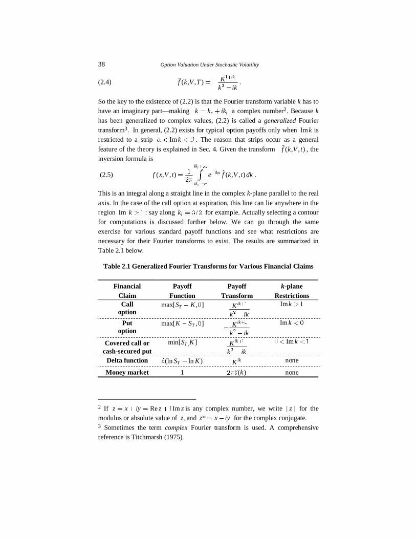
exercise for various standard payoff functions and see what restrictions arenecessary for their Fourier transforms to exist. The results are summarized inTable 2.1 below.

Table 2.1 Generalized Fourier Transforms for Various Financial Claims

FinancialClaim

PayoffFunction

PayoffTransform

k-planeRestrictions

Calloption

max[ , ]TS K� � ikKk ik

�

��

�

�

Imk ��

Putoption

max[ , ]TK S� � ikKk ik

�

��

�

�

Im k � �

Covered call orcash-secured put

,min[ ]TS K ikKk ik

�

�

�

�

Im k� ��

Delta function (ln ln )TS KE � ikK none

Money market 1 ( )kQE� none

2 If Re Imz x iy z i z� � � � is any complex number, we write | |z for themodulus or absolute value of z, and *z x iy� � for the complex conjugate. 3 Sometimes the term complex Fourier transform is used. A comprehensivereference is Titchmarsh (1975).


The delta function. Two of the entries in the table use the Dirac delta function

( )x yE � , which can be thought of as the limit of a function of x that is sharplypeaked at x y� . In the limit, the function is zero everywhere else, whilemaintaining unit area under its “graph”. More rigorously, the delta function is

really a linear “functional” because it transforms well-behaved functions intonumbers via ( ) ( ) ( )x y f x dx f yE

d

�d¨ � � . This function occurs naturally in thetheory; for example, to prove the inversion formula, you insert (2.2) into (2.5)

and rely upon this last equation and < >exp ( ) ( )ikiiki

ik x y dk x yQEd�

�d¨ � � � �� .

Continuing with the development, we next translate (2.1) into a PDE forˆ( , , )f k V t . That’s done by taking the time derivative of both sides of (2.2), and

inside the integral replacing tf by the (negative of the) right-hand-side of (2.1).Then, after parts integrations, the net effect is that x-derivatives of f in (2.1)

become multiplications of f by ( )ik� .

An important point is that we assumed that the boundary terms associated with

the parts integrations can be neglected. This is similar to the issue that wediscovered at (2.3) and led to our introduction of the generalized transform.Typically, there exists a strip Im kB C� � such that the boundary terms

vanish. This is proved in the subsection “Neglected boundary terms” below. It’salso typical that B and C depend upon the parameters of the problem as well,such as the time to expiration. We also show examples of ( )B U and ( )C U below.

With Im k appropriately restricted, the PDE satisfied by ˆ( , , )f k V t is

< > /ˆ ˆ ˆ ˆ ˆ( ) ( ) ( )t V VVf r ik r f V k ik f b ik aV f a fE S� � � � � � � � � ��

� �

�

We remove the dependence on r and E , using T tU � � , and letting

(2.6) < >\ ^ˆ ˆ( , , ) exp ( ) ( , , )f k V t r ik r h k VE U U� � � � .

Also, introducing ( ) ( ) /c k k ik� �� , we see that ˆ( , , )h k V U satisfies the

initial-value problem

(2.7) /ˆ ˆ ˆ ˆ( ) ( ) ( ) ( ) ( )h h ha V b V ik V a V V c k V hVV

SU

s s s ¯� � � �¢ ±s ss

��

� �

�

The initial condition is that ˆ( , , )h k V U � � is given by the Fourier transform of

the payoff function—the entries in Table 2.1.

The fundamental transform. Notice that the entries in Table 2.1 do not depend

upon V. They don’t because we have restricted our theory to volatility


independent payoffs. Because of this assumption, it suffices to take the special

case ˆ( , , )h k V U � �� . To obtain the solution to (2.7) for any other payoff ofthis type, multiply the solution for the special case by the “Payoff Transform”entry in Table 2.1 . This deserves a formal definition and some distinguishing

notation:

Definition. A solution ˆ ( , , )H k V U to (2.7) at a (complex-valued) point k , which

satisfies the initial condition ˆ ( , , )H k V U � �� , is called a fundamental

transform.

Given the fundamental transform, to obtain a (not necessarily unique) solution( , , )F S V t for a particular payoff, here are the steps:

� multiply the fundamental transform by the expiration payoff transform;� further multiply by the factor that we removed in (2.6);� invert the result with the k-plane integration (2.5), keeping Im k in an

appropriate strip; this gives a solution ( , , )f x V t to (2.1);� in terms of S, the solution is ( , , ) (ln , , )F S V t f S V t�

For this procedure to work, we need a strip for which a fundamental solution to(2.7) exists; then we can carry out the inversion along any line contained within.Let’s define a class of problems where this procedure is especially well-defined:

Definition. We call the initial-value problem (2.7) regular4 if there exists afundamental solution to (2.7) which is regular as a function of k within a strip

Im kB C� � , where B and C are real numbers. We call this strip thefundamental strip of regularity. In typical examples, B� � and C � � .

Given the fundamental transform, the steps above are quite straightforward. Foran example using Mathematica, see Appendix 2 to this chapter. For closed-formexamples of the fundamental transform, see Sec. 3 below.

Call option Solution I. The call option payoff transform is given in Table 2.1and it exists for Imk �� . The call option solution in this subsection exists only

under the following assumption: the initial-value problem (2.7) is regular in a

4 A function ( )f k is analytic at a complex-valued point k if it has a derivativethere. If it’s both analytic and single-valued in a region, it’s called regular


strip Im kB C� � and C � � . In other words, we are assuming that the strip

associated with the payoff transform and the fundamental strip intersect. If theydon’t, then this particular solution formula does not exist (but see below—therewill always be an alternative formula that does exist). See Example II below for

an example where there is such an intersection and further examples in Sec. 3.Carrying out the prescription above yields the solution representation

ln ( ) ˆ( , , ) ( , , )i

i

ikr ik

ik S ik rI

ik

e KC S V e e H k V dkk ik

UE UU U

Q

�d� �

� � �

�d

��

¨�

��, Imk C� �� .

We continue to employ T tU � � . This equation can be simplified byintroducing the dimensionless variable

lnr

SeXKe

EU

U

�

�

¯� ¡ °

¡ °¢ ±.

Then, in terms of X, we have Solution I:

(2.8) ˆ ( , , )

( , , )i

i

ik

r ikXI

ik

H k VC S V Ke e dk

k ikU U

UQ

�d

� �

�d

��

¨ �

�

�, Imk C� �� .

Frequently, ˆ ( , , )H k V U is the Fourier transform of a norm-preserving transition

density for the risk-adjusted process. This is discussed further below. For now,we simply note that when H is norm-preserving, then one can show, by Fourierinversion, that

( , , ) ( )rI t TC S V e S KUU � � ¯� �

¢ ±� ,

which is the martingale-style solution. As we will see, sometimes there are othersolutions and sometimes the martingale-style solution is not the arbitrage-freefair value.

Homogeneity. One immediate property of (2.8) is that the call option price ishomogeneous of degree 1 in the stock price and the strike. That is,

( , , ) ( / )C S V K c S KU � . If we multiply both the stock price and the strike bythe same constant: K KMl and S SMl , then C CMl . This is a well-knownconsequence of starting, as we did at Assumption (1.1), with a proportional

stock price process. That is, the (risk-adjusted) stock price return distribution,although dependent upon the initial volatility, is independent of the level of S.5

5 See Theorem 8.9 of Merton (1973).


Call option Solution II. In practice, we often do the k-plane integrations inIm k� �� : usually along /ik � � � . In this strip, H is often free of

singularities—see Example II below and the discussion in Sec. 4. The reason

that this strip is the “regular” one is that solutions to (2.7) are usually quite well-behaved as long as Re ( )c k p � , which is true when Im kb b� � . This strip isespecially important both in the asymptotic U ld behavior of the theory,

which is explained in Chapter 6, and when the martingale-style solution is notthe fair value, which is explained in Chapter 9.

We can obtain a formula for the call option with this restriction by using theput/call parity relation

(2.9) ( , , ) exp( ) [ exp( ) ( , , )]C S V S K r P S VU EU U U� � � � � ,

where ( , , )P S V U is the put option value. The expression in brackets in (2.9) is

the cash-secured put entry in Table 2.1. As you can see from the table, thepayoff function for the cash-secured put has (i) the same Fourier transform asthe call option, except for a minus sign, and (ii) the different restriction

Im k� �� . Now we assume that H is regular in a fundamental strip whichintersects Im k� �� . With that assumption, we have solution II:

(2.10)

In the same way, we define IP to be the put option solution in its natural domainof definition, using Table 2.1:

ˆ ( , , )

( , , )i

i

ik

r ikXI

ik

H k VP S V Ke e dk

k ikU U

UQ

�d

� �

�d

��¨ �

�

�, ImkB� � � .

Again, when ˆ ( , , )H k V U is the Fourier transform of a norm-preserving transitiondensity, then

( , , ) ( )rI t TP S V e K SUU � � ¯� �¢ ±� ,

ˆ ( , , )

( , , )i

i

ik

r ikXII

ik

H k VC S V Se Ke e dk

k ikEU U U

UQ

�d

� � �

�d

� ��¨ �

�

�,

max[ , ] Im min[ , ]kB C� ��


And, using (2.9) and (2.10), we also have the second put option solution in the

same strip as IIC

ˆ ( , , )

( , , )i

i

ik

r ikXII

ik

H k VP S V Ke e dk

k ikU U

UQ

�d

� �

�d

¯¡ °

� �¡ °�¡ °

¢ ±¨ �

��

�

max[ , ] Im min[ , ]kB C� ��

Relationships between the solutions. There is a very simple relationshipbetween the Solution I and Solution II formulas under the assumption that thefundamental strip of regularity for H extends at least slightly above Imk � �

and at least slightly below Im k � � . In that case, one can apply the ResidueTheorem (see Appendix 2.1) to show that

ˆ ( , , )II IC C Se H k i VEU U� ¯� � � �¢ ±�

ˆ ( , , )rII IP P Ke H k VU U� ¯� � � �¢ ±� �

The meaning of these relationships is discussed further below and extensively in

Chapter 9. For now, we simply note that in many situations, the fundamentaltransform is the transform of a norm-preserving transition density that is alsomartingale-preserving. These properties are defined below; when they hold,

then

ˆ ˆ( , , ) ( , , )H k V H k i VU U� � � �� and so II IC C� and II IP P� .

Example I. Constant or deterministic volatility. In the case of constantvolatility, the volatility process is tdV � � and the fundamental transform

satisfies ˆ ˆ( )H c k V HU �� . Applying the initial condition, it’s elementary to find

< >ˆ ( , , ) exp ( )H k V c k VU U� � . This is an entire function of k; i.e., analytic in theentire k-plane. So the only singularities of the integrands in both (2.8) and (2.10)

are simple poles at k � � and k i� . In this case, (2.8) holds for the entire stripIm k� �d� and (2.10) holds for the strip Im k� �� and II IC C� . Of

course, we should recover the B-S formula from both (2.8) or (2.10). This is

shown in the Appendix 2.1 to this chapter.

In the case of deterministic volatility, the volatility process is ( )t tdV b V dt� .

The fundamental transform satisfies ˆ ˆ ˆ( ) ( )VH b V H c k V HU � � . The solution tothis equation is obtained by first finding ( , )Y u V , which is defined as thesolution to / ( )dY du b Y� , ( )Y V�� . Then, the fundamental transform is


given by < >( , , ) exp ( ) ( , )H k V c k U VU U� � , where ( , ) ( , )U V Y u V duU

U ¨��

. So

the k-plane behavior is identical to the case of constant volatility. Again the B-Sformula is recovered, but the volatility V that appears in the formula is replacedby ( , ) ( , ) /V U VU U U�V . Again, see Appendix 2.1

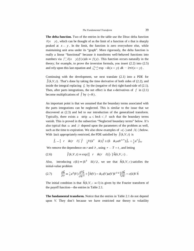
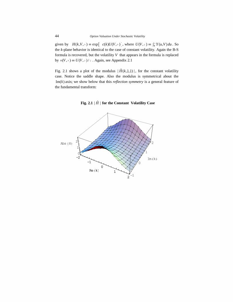
Fig. 2.1 shows a plot of the modulus ˆ| ( , , ) |H k � � , for the constant volatilitycase. Notice the saddle shape. Also the modulus is symmetrical about the

Im( )k axis; we show below that this reflection symmetry is a general feature ofthe fundamental transform:

Fig. 2.1 ˆ| |H for the Constant Volatility Case

-2-1

0

1

2

Re+k/

-1

0

1

2

Im+k/

0

1

2Abs+H/

-2-1

0

1

2

Re+k/


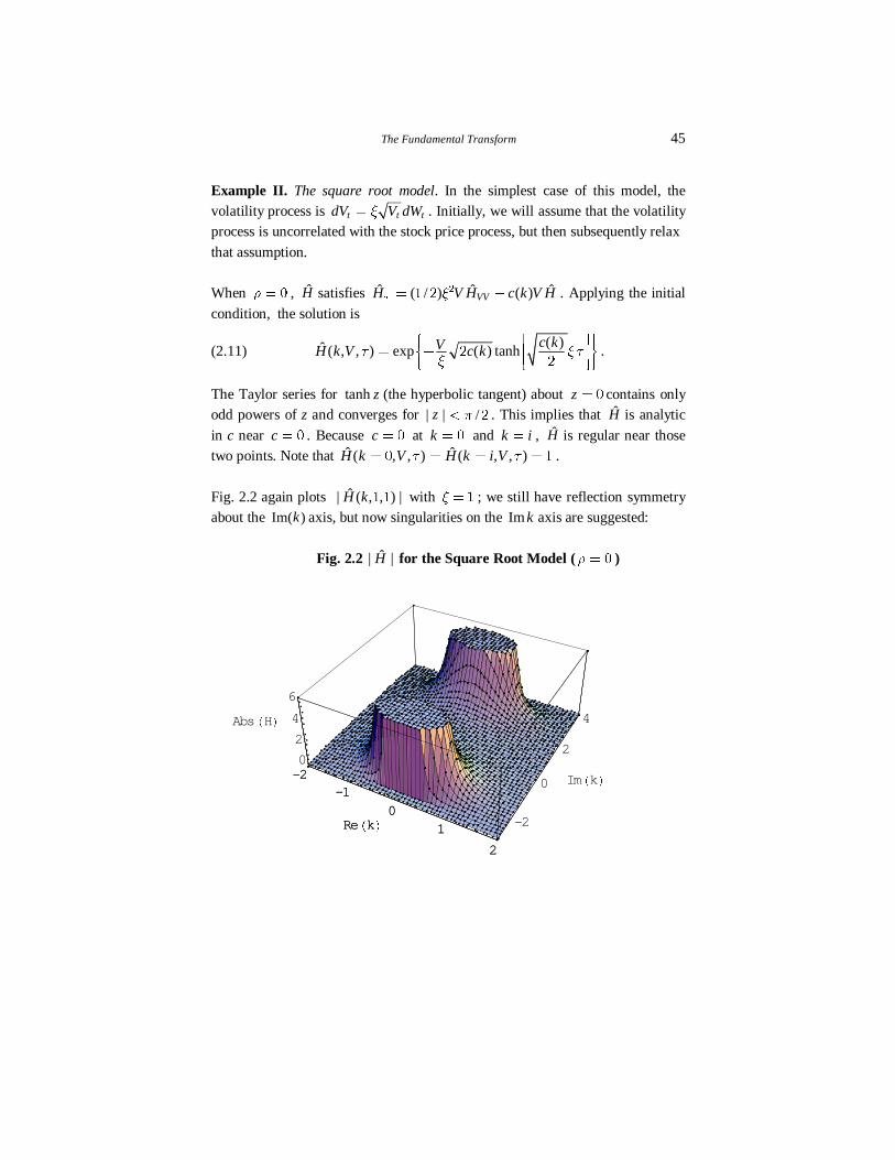
Example II. The square root model. In the simplest case of this model, thevolatility process is t t tdV V dWY� . Initially, we will assume that the volatilityprocess is uncorrelated with the stock price process, but then subsequently relax

that assumption.

When S � � , H satisfies ˆ ˆ ˆ( / ) ( )VVH V H c k V HU

Y� ��

� � . Applying the initial

condition, the solution is

(2.11) ( )ˆ ( , , ) exp ( ) tanh

c kVH k V c kU Y UY

£ ¯ ²¦ ¦¦ ¦¡ °� �¤ »¡ °¦ ¦¦ ¦¥ ¢ ± ¼

��

.

The Taylor series for tanh z (the hyperbolic tangent) about z � � contains onlyodd powers of z and converges for | | /z Q� � . This implies that H is analytic

in c near c � � . Because c � � at k � � and k i� , H is regular near thosetwo points. Note that ˆ ˆ( , , ) ( , , )H k V H k i VU U� � � �� .

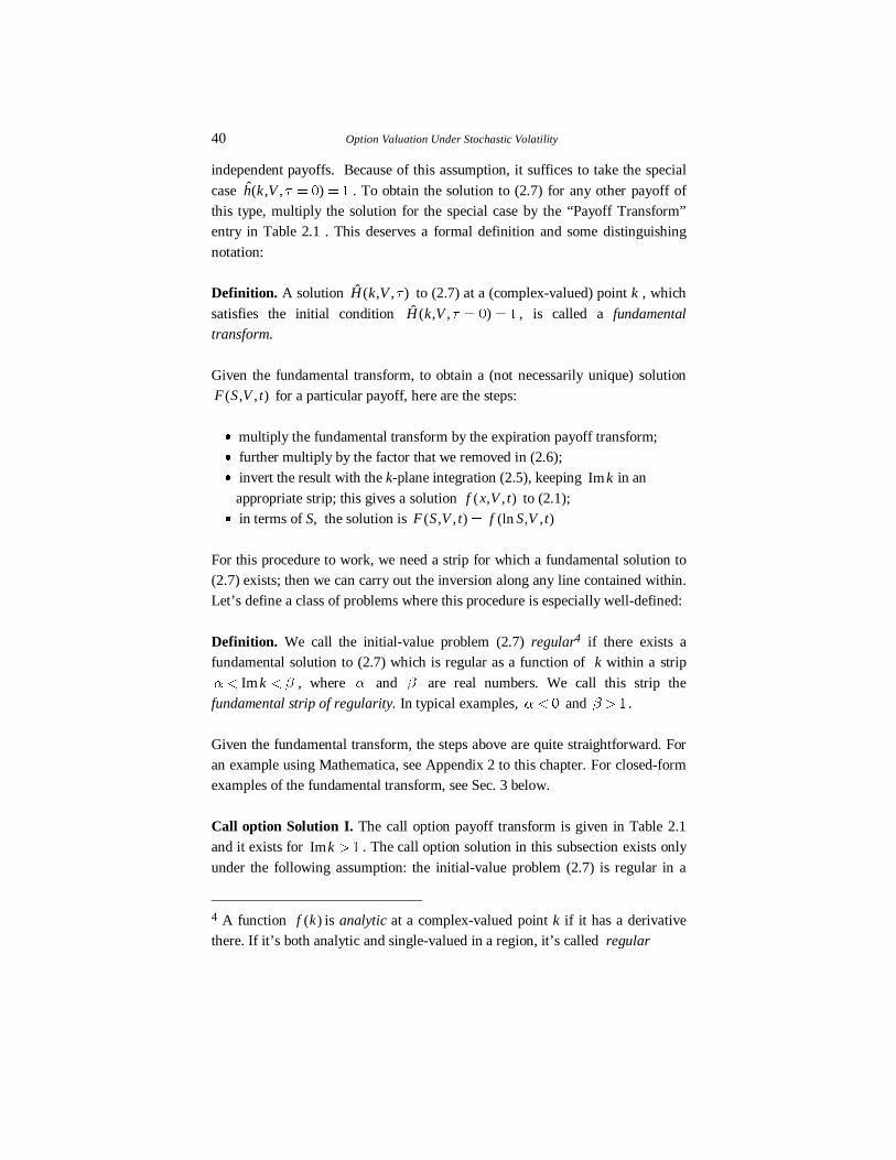
Fig. 2.2 again plots ˆ| ( , , ) |H k � � with Y � � ; we still have reflection symmetryabout the Im( )k axis, but now singularities on the Im k axis are suggested:

Fig. 2.2 ˆ| |H for the Square Root Model (S � � )

-2-1

01

2

Re+k/ -2

0

2

4

Im+k/

0

2

4

6

Abs+H/

-2-1

01

2

Re+k/


Along the pure imaginary axis, let k i y� so that ( ) ( ) /c k y y� � �� . This last

expression becomes negative for y � � or y � � , which means that theargument of the hyperbolic tangent, /( / )c YU� �

� , will be purely imaginary. Sowrite /( / )c iYU K��

� , where K is a real number. But tanh( ) tani iK K�

which will of course diverge whenever ( ) /nK Q� �� , for , , ,n � o o� � �" .Let nk be the locations of the k-plane singularities of H . The singularities inthe figure correspond to the case n � � . Setting /K Q� � , we find

k i yo�� , where .

( ).

y QUY U

o

£¦¦� o � ! ¤¦�¦¥

�

� �

� ��

� � � �� ( )Y U� ��

�

In the limits where Y l�� or U l � , we recover our previous results (an

entire function) because the singularities move off to infinity. In the opposite

limit where Y ld� , the singularities move to ,yo � � � . So as long as Y� isfinite, we see that for this model, the integrand ˆ ( , , ) /( )H k V k ikU �� is free ofsingularities for the strips (i) ImkB� � � (ii) Im k� �� , and (iii)

Imk C� �� , where ( )yB U�� and ( )yC U�� . This is typical.

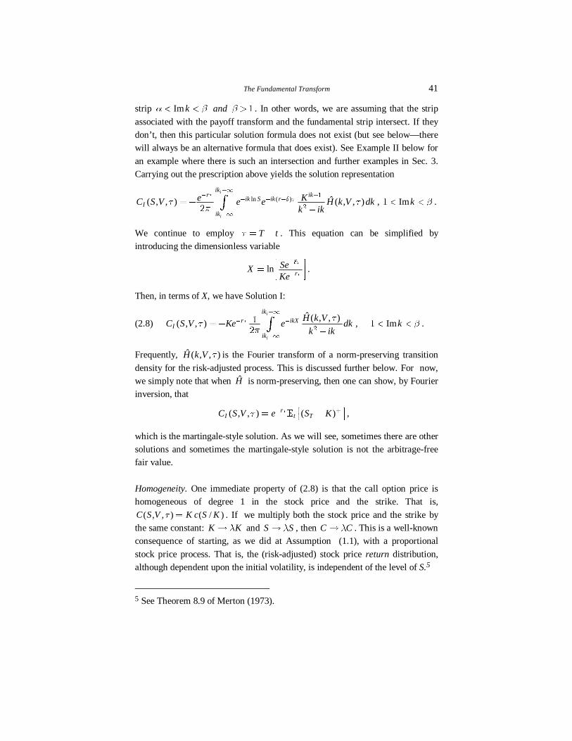
In Fig 2.2, the line Im /k � � � is symmetrically located between the two

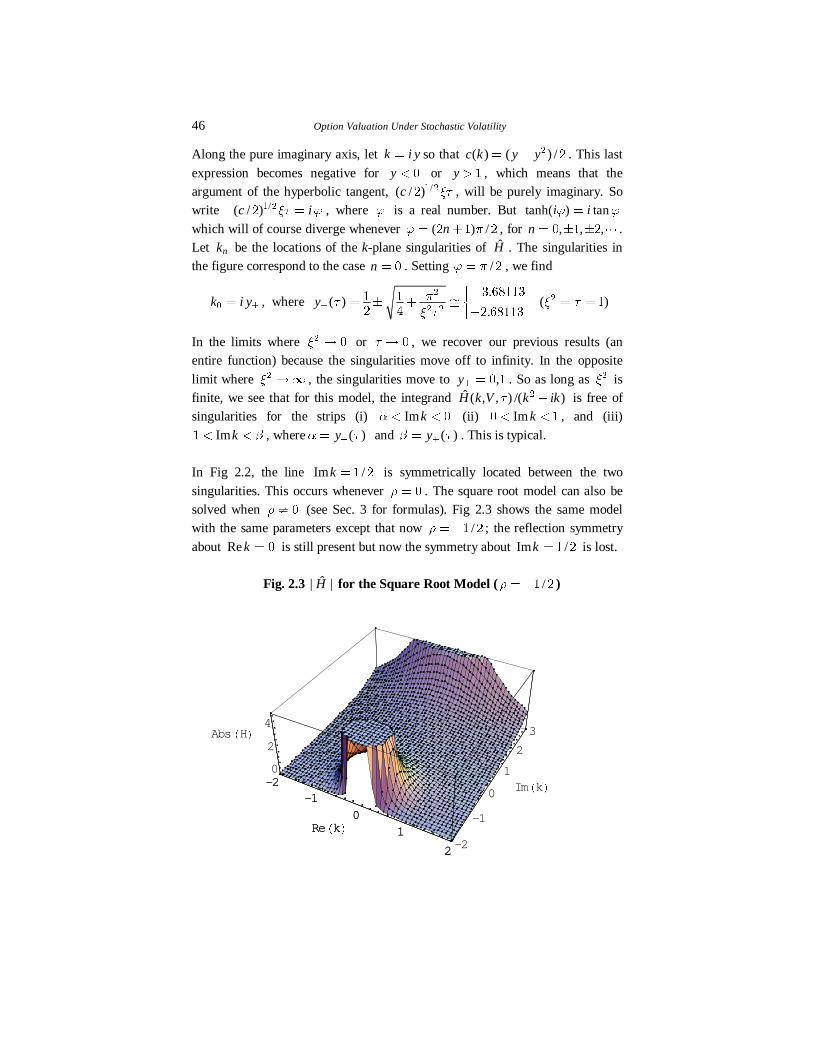
singularities. This occurs whenever S � � . The square root model can also besolved when S v � (see Sec. 3 for formulas). Fig 2.3 shows the same modelwith the same parameters except that now /S �� ; the reflection symmetry

about Re k � � is still present but now the symmetry about Im /k � � � is lost.

Fig. 2.3 ˆ| |H for the Square Root Model ( /S �� )

-2-1

01

2

Re+k/-2

-1

0

1

2

3

Im+k/

0

2

4Abs+H/

-2-1

01

2

Re+k/


A Green function. Consider the entry in Table 2.1 for the delta function claim

(ln ln )TS KE � , but with K � � . From the table, the transform of the payofffunction is 1. So the fundamental transform is a solution to the problem with adelta function payoff and it’s not too surprising that general claims can be

developed in terms of this special one.

A closely related payoff function is ( )TS KE � , which has a fair value which is

sometimes called a Green function or Arrow-Debreu security price. To get fromone delta function to the other, apply the formula

( )

( ( ))| ( ) |

x xf x

f xE

E�

�a

�

�

, where ( )f x �� .

Applying this in our case tells us that

( ) (ln ln )T TS K S KK

E E� � �� .

That is, ( )TS KE � has the payoff transform ikK �� where k is any complex

number. But, for times prior to expiration, we may still have a finite strip wherethe transform exists. So, a solution to the PDE (1.2) for this payoff, which wedenote by ( , , , )G S V K U for Green function, is given by

ln ( ) ˆ( , , , ) ( , , )i

i

ikr

ik S ik r ik

ik

eG S V K e e K H k V dkU

E UU UQ

�d�

� � � �

�d

� ¨ �

�

ˆ ( , , )i

i

ikr

ikX

ik

e e H k V dkK

U

UQ

�d�

�

�d

� ¨�, Im kB C� �

Interpretation of the fundamental transform. The last equation can beinterpreted as follows. Associated with the martingale pricing process (1.1) is arisk-adjusted transition density ( , , , )Tp S V S U� . Specifically Tp dS� is the

probability that the stock price S with instantaneous variance V will, after theelapse of time- U , reach the interval ( , )T T TS S dS� with any variance. Sincethe stock price must end up somewhere, ( , , , )Tp S V S U� is norm-preserving with

respect to TS . That is, ( , , , )T Tp S V S dSUd

¨ ��

�� . Also, we have the initial value( , , , ) ( )T Tp S V S S SE� �� . From the above, we know that both ( , , , )TG S V S U

and ( , , , )Tp S V S U� satisfy the same PDE, (1.1), with the same initial condition.

Are these two functions equal? The answer is yes, if ( , , , )TG S V S U is norm-preserving. As we now show, there is a very simple test to determine when

( , , , )TG S V S U is norm-preserving.


We can simply relabel TK Sl and re-write the last equation, using

ln ( )T

SX rS

E U ¯

� � �¡ °¡ °¢ ±

� , as

(2.12) ˆ( , , , ) ( , , )i

i

ikr

ikXT t

T ik

eG S V S e H k V dkS

U

U UQ

�d�

�

�d

� ¨�

� ,

Inversion. Multiply both sides of (2.12) by exp( )ik Xa� and integrate withrespect to TS from TS � � to TS �d . On the right-hand-side this is

accomplished by changing variables to ln Ty S� and using the delta functionformula given above. The result is

ˆ ( , , ) ( , , , )ikXT TH k V e G S V S dSU U

d

� ¨�

� .

This last formula shows that ˆ ( , , ) ( , , , )T TH k V G S V S dSU Ud

¨� ��

� ; hence

( , , , )TG S V S U is norm-preserving if, and only if, ˆ ( , , )H k V U� �� . That is,we can identify the fundamental transform as the Fourier transform of the norm-preserving transition density in TS if and only if ˆ ( , , )H k V U� �� . In

addition, the last formula shows that the martingale property for the stock price:

( , , , )rT T TSe e S G S V S dSEU U

Ud

� �� ¨�

,

is preserved by G , if and only if ˆ ( , , )H k i V U� � � . These results prompt thefollowing definitions:

Definitions. A fundamental transform ˆ ( , , )H k V U is called norm-preserving if ithas the property ˆ ( , , )H k V U� �� . If a fundamental transform is not norm-

preserving, it’s called norm-defective. A fundamental transform is calledmartingale-preserving if it has the property ˆ ( , , )H k i V U� � � ; otherwise it’scalled martingale-defective.

Examples. The fundamental transform solution for the square root model is bothnorm-preserving and martingale-preserving. The fundamental transform

solutions for the 3/2 model and the GARCH diffusion solution (see Sec. 3 belowand Ch. 11) are sometimes norm-defective or martingale-defective.

With these definitions, we can assert that, when a fundamental transform isnorm-preserving, then it’s the Fourier transform of the risk-adjusted transitiondensity ( , , , )Tp S V S U� ; i.e.,


(2.13)

Failure of the martingale pricing formula. We shall find that it’s possible for

a fundamental transform, in very typical models, to be norm-preserving, butmartingale-defective. Since it’s norm-preserving, it’s the Fourier transform ofthe risk-adjusted transition density ( , , , )Tp S V S U� . In that case, as we noted

earlier, we can interpret call option Solution I as an expectation

( , , ) ( )rI t TC S V e S KU

U� � ¯� �

¢ ±� .

The expectation is taken with respect to the norm-preserving density of the risk-adjusted process: ( , , , )Tp S V S U� . But, as we showed earlier, because the

fundamental transform is martingale-defective, we have a second PDE solution

II IC Cv . Moreover, we show in Chapter 9 that the arbitrage-free fair value isgiven by IIC . In other words, the usual martingale pricing formula

( )rt Te S KU� � ¯�¢ ±

� , while always a solution to the valuation PDE, does not

always give the fair value of an option. Sometimes, option prices are notmartingales, but only strictly local martingales.

Relationship to volatility explosions. When a fundamental transform is norm-

preserving but martingale-defective, we also show in Chapter 9 that

expˆ ˆ( , , ) ( , )H k i V P VU U� � �� , where the right-hand-side is an explosion

probability. Specifically, expˆ ( , )P V U is the probability that a particular volatility

process, the auxiliary volatility process, reaches V ��d prior to time U .

Very briefly, to get a sense of what it going on in these cases, take k i� in (2.7)

and consider solutions to (2.7) expˆ ( , )P V U with vanishing initial condition and

with expˆ ( , )P V U�d � � . If you can find such solutions, the auxiliary process

can explode. Similarly, if the risk-adjusted volatility process can explode, then

there exists a norm-defective fundamental transform such that

expˆ ( , , ) ( , )H k V P VU U� � �� , where the right-hand-side is the explosion

probability for the risk-adjusted process. In this case, take k � � in (2.7) Again,

see Chapter 9 for a detailed discussion.

ˆ ( , , ) ( , , , )ikXT TH k V e p S V S dSU U

d

� ¨�

�

� ,

where ln ( )T

SX rS

E U ¯

� � �¡ °¡ °¢ ±

� ,

if and only if ˆ ( , , )H k V U� ��


Reflection symmetry. Note that we always have the property, because the

fundamental transform is the transform of a real-valued function,*ˆ ˆ( , , ) ( *, , )H k V H k VU U� � . This always holds, whether or not the transform is

defective.

With the exception of the results for the 3/2 model given in Sec. 3 below, wegenerally assume without further comment that for the remaining development

in this chapter, the fundamental transform is both norm- and martingale-preserving.

Power law behavior and scaling. Since X� is a function of the ratio / TS S ,then (2.13) shows that the transition density satisfies the scaling behavior

(2.14) ( , , , ) ( )TT

p S V S uS

U K��

� , where / Tu S S� ,

and ( )uK is some scaling function. So if we know the behavior of ( , , , )Tp S V S U�

for , ( )T TS Sld l � then we also know the behavior as, ( )S Sl ld� respectively. In fact, if the problem is regular, then we can

deduce a lot about that behavior. For example, (2.13) exists for k iy� ,

where y C F� � for every F� � . That is, for any S � �

( , , , )T TTS p S V S dSC FU

d� �d¨

�

� .

This implies that ( , , , ) ( )T Tp S V S O S C FU

� � �� as TS ld , for every F� � .

Similarly, taking y B F� � implies that ( , , , ) ( )T Tp S V S O S B FU

� � �� as

TS l � 6. In turn, these relations may be restated in terms of the scalingfunction:

(2.15) ( ) as

( )( ) as

O u uu

O u u

C F

B FK

�

� �

£¦ l¦� ¤¦ ld¦¥

�for every F� � .

Neglected boundary terms. One application of (2.14) is to show that theneglected boundary terms associated with the call option solution (2.8) canindeed be neglected. Writing ( ) ( , , )xf x C e V t� , where lnx S� , the two

neglected boundary terms from parts integrations were

6 The notation, as x xl � , ( ) ( )f x O g x� , means that ( ) / ( )f x g x isbounded as x xl � . For a more rigorous discussion of the power law order

behavior for p� , see Fourier’s theorem for analytic functions (Titchmarsh 1975,Theorem 26, p.44)


( )xikxx

e f x��d

��d and

( ) xikx

x

f xe

x

��d

��d

s

s where Imk C� ��

In Appendix 2.3 to this chapter, we show the general arbitrage boundsxC S eb � , and SC b� , which implies that both xf eb and / xf x es s b for

large enough x. So, since Imk �� , both boundary terms vanish at the upper

limit x ��d .

When option prices are martingales, they are given by the pricing formula

( , , ) ( , , , ) max[ , ]rT T TC S V e p S V S S K dSUU U

d�� ¨

�

��

/

( )S K

r K due S u uS u

U K� ¯� �¡ °¢ ±¨ �

�

� ,

where we substituted from (2.14). Letting S l � , we have from (2.15) that( ) ( )u O uC FK �� as u l � . Substituting this expression into the above integral

implies that ( ) ( )C S O SC F�� as S l � for every F� � . Or, in other wordsboth ( )( )xf O e C F�� and ( )/ ( )xf x O e C F�s s � as x l�d . Since Imk C� ,both boundary terms also vanish at the lower limit x ��d . �

The fundamental transform as a characteristic function. By a characteristicfunction, we mean any function that has the form

(2.16) ˆ ( ) ( ) ( )ikx ikxH k e dG x e g x dxd d

�d �d

� �¨ ¨ ,

where ( )G x is a cumulative distribution function and ( ) /g x dG dx� is itsprobability density. For our purposes in this chapter, a cumulative distributionfunction is function of a real variable x that is (i) non-decreasing, and (ii)

satisfies ( )G �d � � , ( )G �d � � . Of course, for this to occur, then( )g x must be non-negative and integrable.

To show that H is a characteristic function, change integration variables in(2.13) from TS to ln( / ) ( )TX S S r E U� � �� and define a new function

( ; , , )g X S V U� by

( )( , , , ) ( ; , , )r XTp S V S S e g X S VE UU U� � �

�

�

� .

Or, suppressing arguments again,

( ) ( )( ) ( ) , , ,r X r XdG X g X dX p S V Se S e dXE U E UU� � � ��

� � � �

� .

This shows that ( )H X� is non-negative and now (2.13) reads


ˆ ( ) ( )ikXH k e dG Xd

�d

� ¨�

� ,

where ( ) ( )( ) , , ,X

r x r xG X p S V Se S e dxE U E UU

� � � �

�d

� ¨�

�

�

< >exp ( )

, , ,T T

S r X

p S V S dSE U

U

d

� �

� ¨�

� .

This last equation shows that ( )G X� is indeed non-decreasing and satisfies( )G �d � � , ( )G �d � � . And, since ˆ ( )H k is of the form (2.16), with

x X� � , this shows that ˆ ( )H k is a characteristic function. In fact, the examples

show that ˆ ( )H k can typically be further characterized as an analytic

characteristic function. This important topic is discussed in Sec. 4.

The martingale pricing density. We can also consider the probability density( , , , )t t Tp S V S U that the actual volatility process, starting from ( , )t tS V reaches

TS with any variance. The ratio of the two probabilities

( , , , )

( , , , )( , , , )

t t Tt t t T

t t T

p S V SM M S V S

p S V SU

U

U

� �

�

also values arbitrary payoffs. That is, we have two general pricing formulas thatwork for any volatility-independent claim price, when it’s a martingale:

(2.17) ( , , ) ( , , , ) ( )rt t t t T T TF S V e p S V S g S dSU

U U

d

�

� ¨�

�

( , , , ) ( , , , ) ( )rt t T t t T T Te M S V S p S V S g S dSU

U U

d

�

� ¨�

.

These are explicit integral kernel versions of the martingale pricing formulaspresented in Chapter 1. As a general rule, (2.17) is the long way around,however, from the Solution I and II formulas based upon a direct k-plane

integration, since it forces you to do an extra integration. So we don’trecommend (2.17) for most computations—but we have seen already that it wasuseful in considering the S l � and S ld limits of the theory.

Forward contracts and options on forwards. The formulas are easilymodified to handle forwards. For example, the forward stock price tF is defined

to be the fair value at time t for delivery of one share of the stock at time T . Asusual, this price is determined by arbitrage to be ( )r

t tF e SE U�

� , whereT tU � � . Hence by Ito’s formula, the martingale pricing process P� of (1.1)

becomes t t t tdF F dBT� � , with the same volatility evolution. Under P� , the


forward price behaves like a stock with a dividend yield of r. Using this idea, a

call option on the forward, say solution II at Im /k � � � , becomes

/

/

ˆ ( , , )( , , )

i

r ikXII

i

H k VC F V e F K e dk

k ikU

U

U

Q

�d

� �

�d

¯¡ °

� �¡ °�¡ °

¢ ±¨�

�

�

�

�,

where ln /X F K� .

Summary. If the initial-value problem in the box below is regular in a stripIm kB C� � in the complex k-plane, then the solution can be used to

determine option prices by a k-plane integration:

3 Some Models with Closed-form Solutions

In general, even with the assumption of a simple process for the actual

volatility, the simplest risk-adjustments (via utility theory) can produce complex

results for the martingale pricing process. Risk-adjustment is discussed in detailin Chapter 7. To obtain a model that can be solved in closed-form generallyrequires two assumptions: (i) a relatively simple process for the actual volatility,

and (ii) a relatively simple preference model, such as the representative agentmodel with power utility.

Making both of these assumptions, here is a short list of models that can besolved in closed-form. Each volatility process has constant correlation S with

(2.19) /ˆ ˆ ˆ ˆ( ) ( ) ( ) ( ) ( )H H Ha V b V ik V a V V c k V HVV

SU

s s s ¯� � � �¢ ±s ss

��

� �

�

where ( ) ( ) /c k k ik� �� . In addition to ˆ ( , , )H k V U � �� , the

fundamental solution has the following properties:

(2.20) (i) *ˆ ˆ( , , ) ( *, , )H k V H k VU U� �

(ii) expˆ ( , , ) ( , )H k V P VU U� � ��

(iii) expˆ ˆ( , , ) ( , )H k i V P VU U� � �� ,

where expP and expP are the probabilities that the auxiliary volatility

process and risk-adjusted volatility process can explode to �d


the stock price process. All other parameters are also constants. The agent is

assumed to be a pure investor (no consumption until a final date) with a distantplanning horizon. The parameter H is the representative’s risk-aversionparameter. It’s restricted to H b� plus some additional restrictions that are

shown. The risk-aversion adjustments are derived in Chapter 7.

Some solvable models and their volatility processes

Square root model

: ( )P dV V dt V dWX R Y� � �

\ ^: P dV V dt V dWX R Y� � �� ,

where ( ) ( )R H SY R H H Y� � � � ��

Conditions: ( )H H R� b ��

3/2 model

/: ( )P dV V V dt V dWX R Y� � ��

\ ^ /: P dV V V dt V dWX R Y� � �� ,

where ( ) ( ) ( )R Y H SY R Y H H Y��

� ��

Conditions: ( ) ( )H H Y R Y� b ��

��

Geometric Brownian motion

: P dV V dt V dWR Y��

/ ( ): ( )

( )K y

P dV V V y dt V dWK yN

N

H S Y Y Ya£ ¯ ²¦ ¦¦ ¦¡ °� � � � � �¤ »

¡ °¦ ¦¦ ¦¥ ¢ ± ¼

� � ��

�� ,

where ( )y VH HY

� � �� and RN

Y� �

�

�� .

Conditions: ( R Y� � �� and H b � ) or H � �

The solution for the fundamental transform under geometric Brownian motion isquite complex and difficult to work with when the correlation is non-zero. In

contrast, both the square root model and the 3/2 model have short solutions thatwe now show. Both models use the reduced variables


(3.1) t Y U� ��

�, X X

Y�

�

�� , ( )c c k

Y�

�

�� .

In terms of these variables, the fundamental transforms are given below. Theresults for all three models are derived in Chapter 11.

The square root model7 [H b� and ( )H H Y R� b� �� ]

(3.2) < >ˆ ( , , ) exp ( ) ( )H k V f t f t VU � �� , using

exp( )( ) ln

h d tf t t g

hX

¯�� ¡ °

¡ � °¢ ±�

�

�� ,

exp( )( )

exp( )d t

f t gh d t

� ¬� �� ®��

�

�

/ˆ[ ]d cR� �� , ˆ( )g dR� ��

�,

ˆˆ

dhd

R

R

��

,

where ˆ( ) ( ) ( )k ikR H SY R H H YY

¯� � � � � �¡ °¢ ±� �

�

��

The 3/2 model8 [ H b� and ( ) ( )H H Y R Y� b ��

�� ]

(3.3) ( )ˆ ( , , ) , , , , ( )

H k V X M XV V

BC B X XU X U B C X UC

( � ¯ ¯� �¡ ° ¡ °( ¢ ± ¢ ±� � ,

using ( , )txX x t

e�

��, ˆ( )N R� ��

�� ,

/cE N ¯� �¢ ±

� ��

� ,

B N E�� , C E� �� ,

where ˆ( ) ( ) ( ) ( )k ikR R Y H H Y H SYY

¯� � � � � � � � �¡ °¢ ±� � ��

��

�� .

7 Heston’s (1993) call option solution is also achieved with a transform-basedapproach: an ordinary Fourier transform with respect to the log-strike price. In

Heston’s approach, there are two transforms instead of the one here.8 Caution: this fundamental transform is sometimes either norm-defective ormartingale-defective. Using risk-neutral preferences only, the 3/2 model has

been independently developed by Heston (1997), using an approach similar tohis 1993 paper.


In (3.3), ( )z( is the Gamma function and ( , , )M zB C is a confluent

hypergeometric function9 . Also, note that the second argument for ( , )X t t in(3.3) uses tX U X� � .

Determining the fundamental strip. Once you have H for a model, then youcan analyze it to determine the fundamental strip of regularity: Im kB C� �

and whether it’s norm- and/or martingale-preserving. Once you know that, you

know the regions of validity for all of the option formulas presented previously.As an example, consider the square root model above. Rather than a completeanalysis, let’s just establish that the strip Im k� �� is free from

singularities—this places the boundaries of the fundamental strip outside thisregion.

The singularities occur where dthe�� , which causes divergences in both ( )f t�

and ( )f t� . We know the singularities occur along the imaginary axis, soconsider k iy� , where y is real. We see from (3.1) that R� is real along that

axis. Moreover, for Im k� �� , then c � �� (and real). Hence d is real andsatisfies | |d R� � , which implies that dR � � �� and dR � � �� . In other words,

h � � . Since d is real and h � � , there can be no solutions to dth e�� inside

the strip Im k� �� . Hence Im k� �� is free from singularities. �

Integrating. Once you know where you can legally integrate, then you’re a k-

plane integration away from the call option price. For these remaining steps, seeAppendix 2.2 to this chapter. When you obtain those prices, you’ll find that bothmodels exhibit the typical qualitative behavior that we discuss in subsequent

chapters: implied volatility smile patterns (see Chapter 5) and an impliedvolatility term structure that flattens to a constant as U ld (see Chapter 6).For the derivation of the formulas (3.2) and (3.3) see Chapter 11.

4 Analytic Characteristic Functions

We have seen from examples that ˆ ( , , )H k V U is often an analytic function of k in

some neighborhood. In general, a characteristic function ˆ( )f k is any functionwhich has the representation 9 See Abramowitz and Stegun (1970) for properties of these and other specialfunctions.


ˆ( ) ( )ikxf k e p x dxd

�d

� ¨ ,

where ( )p x is a probability density for some cumulative distribution function.

Lukacs (1970, Chapter 7) proves two theorems that are relevant to ourapplication. To achieve a more symmetrical notation, we write ˆ ( )H k for ourfundamental transform and ˆ( )f k for a generic characteristic function

If ˆ( )f k is regular in a neighborhood of k iy� , where y is real, then we callˆ( )f k an analytic characteristic function (Lukacs takes y � � ). We have shown

in a number of examples that the regions of regularity for ˆ ( )H k are typicallystrips in the complex k-plane. And, we have suggested strips as regions ofregularity in general. The rationale for the general case lies in the following

theorem, quoted without proof:

THEOREM 2.1 (Lukacs Theorem 7.1.1): If a characteristic function ˆ( )f k is

regular in the neighborhood of k � � , then it is also regular in a horizontal

strip and can be represented in this strip by a Fourier integral. This strip is

either the whole plane, or it has one or two horizontal boundary lines. The

purely imaginary points on the boundary of the strip of regularity (if this strip is

not the whole plane) are singular points of ˆ( )f k .

Discussion. In our application, we have often found that the fundamentaltransform ˆ ( )H k is regular in the horizontal strip Im kB C� � , where B� �

and C � � . We have already pointed out that the PDE (2.19) is especially well-

behaved when Re ( )c k � � , which occurs when Im k� �� . In thissubsection, we try to understand a little better why the strip Im k� �� isoften free of singularities of ˆ ( )H k . We know from (2.13) that ˆ ( )H k has the

representation

( )ˆ ( , , ) ( , , , )TikX ST TH k V e p S V S dSU U

d

� ¨�

�

� ,

where ( ) ln ( )TT

SX S rS

E U ¯

� � �¡ °¡ °¢ ±

� . Therefore

< >( )ˆ ˆ( ) ( ) ( ) ( , , , )m mm m ikX

T T TmdH k H k i X S e p S V S dSdk

Ud

� � ¨�

�

�

� .

Let rk k i y� � , where rk and y are real. Then,

< > ( ) ( )ˆ ( ) ( ) ( , , , )r

ymm m y r ik X T

r T T TS

H k i y i e X S e p S V S dSS

E U Ud

� �� ¨�

�

�

�


Along the purely imaginary axis, we have

(4.1) < > ( ) ( )ˆ ( ) ( ) ( , , , )y

mm m y r TT T T

SH i y i e X S p S V S dS

SE U

U

d� �� ¨

�

�

� .

And in particular for the fundamental transform itself, we have

(4.2) ( )ˆ ( ) ( , , , )y

m y r TT T

SH i y i e p S V S dS

SE U

U

d� �� ¨

�

� .

Now it’s known from complex variable theory that if a function is analytic in aregion R, then it has derivatives of all orders and a Taylor series in R.

Consequently, if ˆ ( )H k is regular near the point k iy� , then the series

( )ˆ ( )ˆ ( ) ( )

!

mm

m

H iyH k k iy

m

d

�

� ��

is convergent. This means that ˆ ( )H k is an analytic characteristic function neark iy� if and only if the following two conditions are satisfied:

(4.3) (i) ( )ˆ ( )mH iy exists for all , , ,m � � � �!

(4.4) (ii) /( )ˆ| ( ) |

lim !

mm

m

H iymld

¯¡ ° �¡ ° %¢ ±

�

� is finite.

Then if these conditions hold, ˆ ( )H k is regular in the strip( ) Im ( )y k y�% � � �% .

Now recall the normalization and martingale identity:

(a) ( , , , )T Tp S V S dSU

d

�¨�

�� and (b) ( , , , )rT T TSe e S p S V S dSEU U

U

d� �� ¨

�

� .

These two relations strongly restrict the possible behavior of ( )Tp S� near

TS � � and TS �d , where we suppress the other arguments in

( , , , )Tp S V S U� . Because of (a), it must be true that ( ) ( )T Tp S O S F� �� for every

F� � as TS l � . In other words ( )Tp S� , if it diverges at all as TS l � ,diverges no faster than TS F� �� . Similarly, because of (b), it must be true that

( ) ( )T Tp S O S F� �� for every F� � , as TS ld . Because of these two end-

point behaviors, if you keep y in (4.2) in the range y� �� , then you willhave a convergent integral. Similarly, with the same restriction, (4.1) should

exist for any m because, (I) as x ld , | ln( / ) | ( )y mx x O x�� for any y � �

and (II) as x l � , | ln( / ) | ( )y mx x O�� for any y � �


Unfortunately, this argument establishes (4.3) but not (4.4). Nevertheless, it

provides some additional insight into why Im k� �� is the “natural” strip forthe financial claim problem.

Stationary points. In Chapter 6, “The Term Structure of Implied Volatility”, weexamine the asymptotic U ld behavior of the theory. It turns out that theasymptotic implied volatility is determined by an eigenvalue of a differential

operator. This eigenvalue is also a stationary or saddle point of ˆ ( )H k in the k-plane (recall the saddle shapes from the figures). We discover, in particularmodels, that these stationary points always lie along the purely imaginary axis.

The general reason for this behavior lies in the following theorem:

THEOREM 2.3 (Lukacs Theorem 7.1.2): Let ˆ( )f k be an analytic characteristic

function. Then ˆ| ( ) |f k attains its maximum along any horizontal line contained

in the interior of its strip of regularity on the imaginary axis. The derivativesˆ /j jd f dk� � of even order of f have the same property.

PROOF: We know that ˆ( )f k has the representation

ˆ( ) ( )ikxf k e p x dxd

�d

� ¨ , Im kB C� � .

Therefore ( )ˆ ˆ( ) ( ) ( )m

m m m ikxm

df k f k i x e p x dxdk

d

�d

� � ¨ .

Let rk k i y� � , where rk and y are real and where yB C� � . Then,

( )ˆ| ( ) | | | ( )m m yxrf k i y x e p x dx

d�

�d

� b ¨ .

If m j� � ( , , , )j � � � �! is an even integer, then this becomes

( ) ( )ˆ ˆ| ( ) | ( ) | ( ) |j j yx jrf k i y x e p x dx f i y

d�

�d

� b �¨� � � ,

so that ( ) ( )ˆ ˆmax | ( ) | | ( ) |r

j jr

kf k i y f i y

�d� �d

� �� .

The ridge property. The relation

ˆ ˆ| ( ) | | ( ) |rf k i y f i y� b

is very important in the theory of analytic characteristic functions, and is called

the “ridge property”. It plays an important role in our application in theasymptotic U ld theory. So we have learned that if the fundamental


transform ˆ ( )H k is an analytic characteristic function, then it is also a “ridge

function”.

Documents

Option Valuation under Stochastic Volatility With ... · In this chapter we introduce a transform-based approach to solving the option valuation PDE that we ... a pure investor model