Real Option Valuation

Antoinette SchoarMIT Sloan School of Management

15.431

Spring 2011

Spotting Real (Strategic) Options

• Strategic options are a central in valuing new ventures → Option to expand → Option to delay → Option to abandon → Option to get into related businesses

• Different approaches to valuing real options → Decision analytic approach → Binomial method → Black- Scholes model

Real Options in Traditional Valuation Methods

• Where are real options in DCF Method? → No where!

• Where are real options in Venture Capital Method? → Valuations might be based entirely on real option value if the

market prices these in → But we have no way to know whether the market has

correctly accounted for real options

Example: Option to Enter New Markets

• Consider the strategy of Focal Communications, a Competitive Local Exchange Carrier (CLEC) circa 1996.

• Could choose to enter all local markets simultaneously or could enter local markets sequentially.

• Advantage of Sequential Entry: You get to see how valuable it is to be a CLEC before deciding whether to enter more markets. → New information is obtained by entering the first market, and

management adjusts its strategy in response.

Example of “Real Options” Analysis

• Suppose the key source of uncertainty is the markup of price over carrier settlements.

• Suppose that there is a 50% chance that the mark up is high (25% mark up) and a 50% chance that it is low (15% mark up).

• Assume the expected value of entering a market is $13.9 million if the mark up is high and -$5.9 million if the mark up is low

• The firm can enter 10 markets

• How would you model this uncertainty?

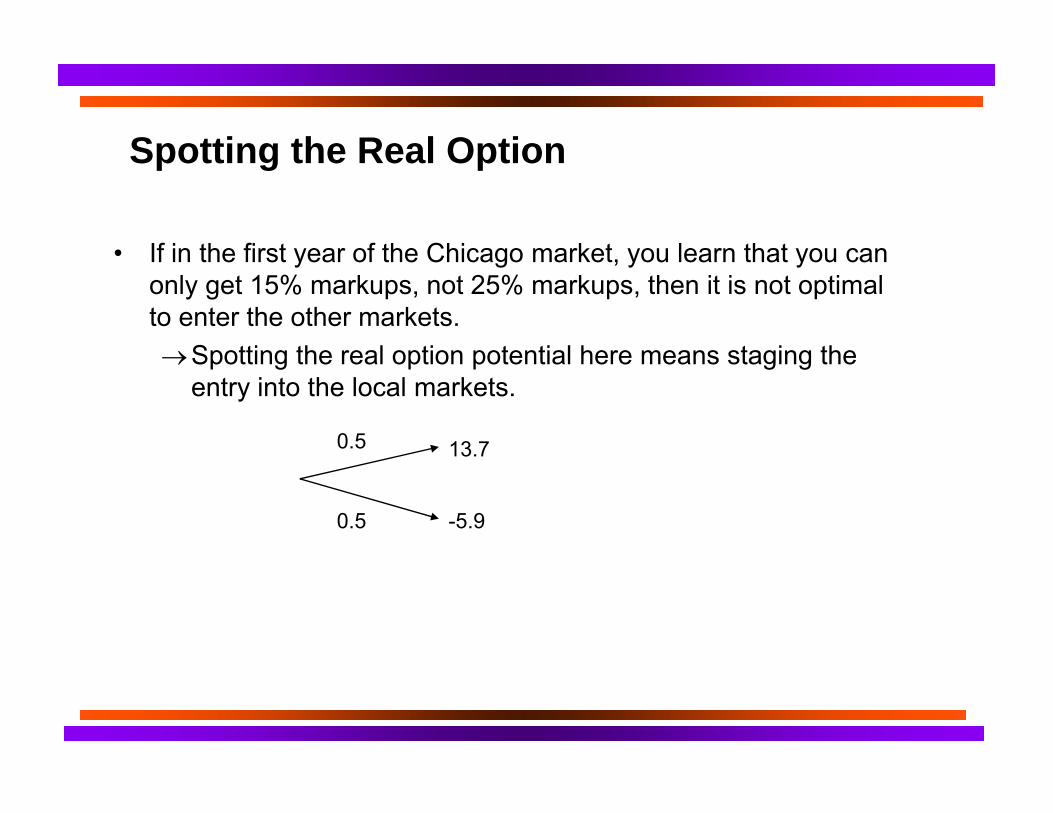
Spotting the Real Option

• If in the first year of the Chicago market, you learn that you can only get 15% markups, not 25% markups, then it is not optimal to enter the other markets. → Spotting the real option potential here means staging the

entry into the local markets.

0.5 13.7

0.5 -5.9

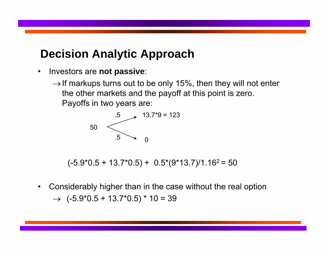
Decision Analytic Approach • Investors are not passive:

→ If markups turns out to be only 15%, then they will not enter the other markets and the payoff at this point is zero. Payoffs in two years are:

.5 13.7*9 = 123

50

.5 0

(-5.9*0.5 + 13.7*0.5) + 0.5*(9*13.7)/1.162 = 50

• How does it compare to scenario analysis?

Decision Analytic Approach • Investors are not passive:

→ If markups turns out to be only 15%, then they will not enter the other markets and the payoff at this point is zero. Payoffs in two years are:

.5 13.7*9 = 123

50

.5 0

(-5.9*0.5 + 13.7*0.5) + 0.5*(9*13.7)/1.162 = 50

• Considerably higher than in the case without the real option → (-5.9*0.5 + 13.7*0.5) * 10 = 39

What About Valuing Real Options a la Black-Scholes?

• As long as we know the volatility of the underlying value, the interest rate, the time horizon, and today’s market value, we’re all set.

• Plug and Chug!?

No Way!

• Analogy between financial and real options is less than perfect.

• To apply financial options pricing methodology to real options and understand its strengths and weaknesses, we need to review the underlying assumptions and mechanics.

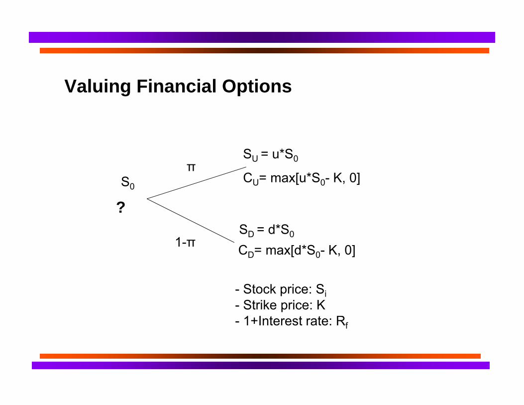
Valuing Financial Options

SU = u*S0π

S0 CU= max[u*S0- K, 0]

? SD = d*S0

1-π CD= max[d*S0- K, 0]

- Stock price: Si - Strike price: K - 1+Interest rate: Rf

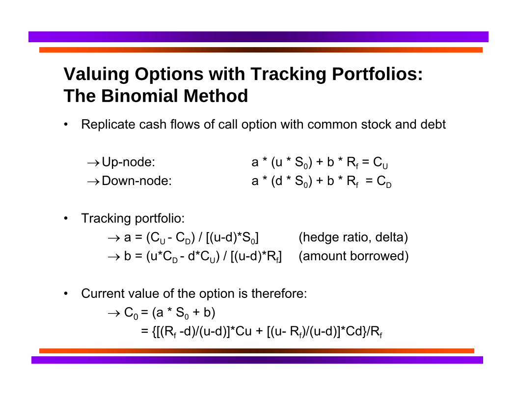
Valuing Options with Tracking Portfolios: The Binomial Method • Replicate cash flows of call option with common stock and debt

→ Up-node: a * (u * S0) + b * Rf = CU

→ Down-node: a * (d * S0) + b * Rf = CD

• Tracking portfolio: → a = (CU - CD) / [(u-d)*S0] (hedge ratio, delta) → b = (u*CD - d*CU) / [(u-d)*Rf] (amount borrowed)

• Current value of the option is therefore: → C0 = (a * S0 + b)

= {[(Rf -d)/(u-d)]*Cu + [(u- Rf)/(u-d)]*Cd}/Rf

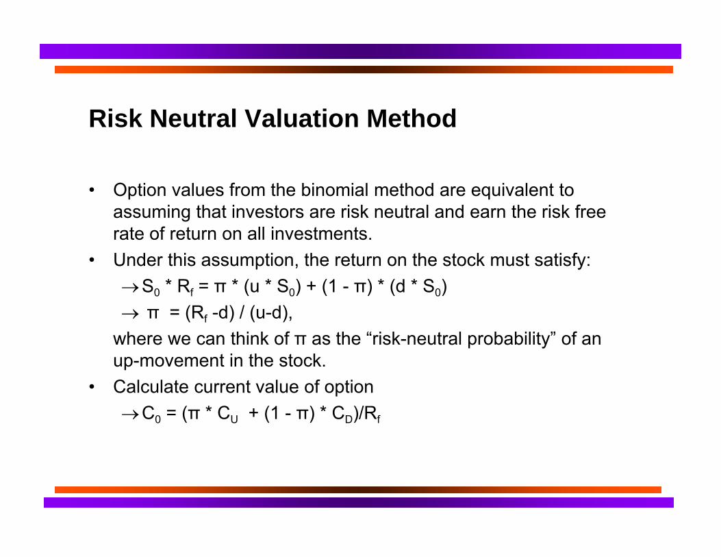
Risk Neutral Valuation Method

• Option values from the binomial method are equivalent to assuming that investors are risk neutral and earn the risk free rate of return on all investments.

• Under this assumption, the return on the stock must satisfy: → S0 * Rf = π * (u * S0) + (1 - π) * (d * S0) →π = (Rf -d) / (u-d),

where we can think of π as the “risk-neutral probability” of an up-movement in the stock.

• Calculate current value of option → C0 = (π * CU + (1 - π) * CD)/Rf

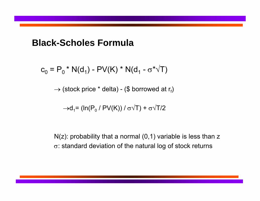
Black-Scholes Formula

c0 = P0 * N(d1) - PV(K) * N(d1 - σ*√T)

→ (stock price * delta) - ($ borrowed at rf)

→d1= (ln(P0 / PV(K)) / σ√T) + σ√T/2

N(z): probability that a normal (0,1) variable is less than z σ: standard deviation of the natural log of stock returns

Where are Probabilities/Expected Returns in Financial Option Pricing Formulas?

• Expected stock returns (future stock price) do not explicitly enter into the option pricing formula.

• The stock price today incorporates all the necessary information about expected stock returns. It reflects the average investor’s valuation of the probability distribution of future stock prices

Using Option Pricing Methodologies to Value Real Options?

• How do we translate key variables into real options?

• rf = Time value of money • t = Length of time till option has to be realized • K = Expenditure required to acquire project assets • σ = Riskiness of project • S0 = Present value of project

How to Get Variables for Option Pricing

• Use DCF valuation analysis to get present value • Use scenario analysis to get volatility of present value

→ Need to make assumptions about probabilities of various outcomes

→ Need to make assumptions about the cash flows under different scenarios

→ If you have volatility of comparable company you might be able to use these. But rarely available

Difficulties in Applying Option Pricing Methodologies to New Ventures

• Present value of project? Riskiness? → Underlying project is not traded and therefore its market

value is not immediately known → Returns might not be normally distributed → Real options lead to real decisions! These affect the future

value of the project itself

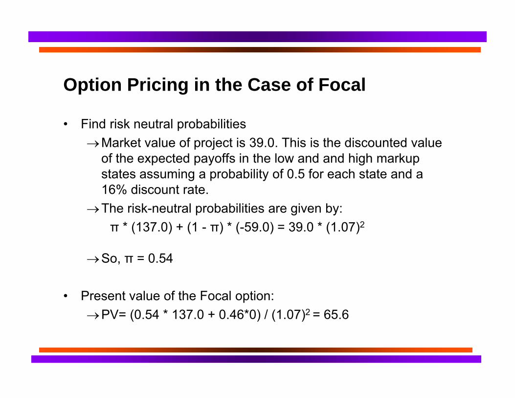
Option Pricing in the Case of Focal

• Find risk neutral probabilities → Market value of project is 39.0. This is the discounted value

of the expected payoffs in the low and and high markup states assuming a probability of 0.5 for each state and a 16% discount rate.

→ The risk-neutral probabilities are given by:π * (137.0) + (1 - π) * (-59.0) = 39.0 * (1.07)2

→ So, π = 0.54

• Present value of the Focal option: → PV= (0.54 * 137.0 + 0.46*0) / (1.07)2 = 65.6

Decision Analysis vs. Option Pricing

• The Option Pricing Method gives a higher valuation than the Decision Analysis Method (65 vs. 50).

• Note that you need the same information to price the options using both methods.

• Both methods have their drawbacks → The Option Pricing Method assumes that there is arbitrage

when there clearly isn’t → The Decision Analysis Method discounts payoffs using

CAPM-based discount rates which assume that payoffs are linear.

What to Do • It is important to spot the option and to get some rough sense of its

value.

• Understand what is the critical part of the existing project that generates the real option → Real options have to be embedded in the first step, otherwise you

do not need the first part. Then it is not a real option anymore but an opportunity!

• Be careful when pricing real options with the Black & Scholes formula →Volatility of underlying project is difficult to estimate →Misestimating the volatility of an option can severely affect its value

What not to do

• Don’t use options opportunistically: Sometimes people use real options as ex post justification of bad investment decisions!

• “This business may look bad, but it gives us options to get into better businesses.” → A bad project is still a bad project. Avoid it if you can!

MIT OpenCourseWare http://ocw.mit.edu

15.431 Entrepreneurial Finance Spring 2011

For information about citing these materials or our Terms of Use, visit: http://ocw.mit.edu/terms.