Optimizing Inbound Freight Mode Decisionsby

Colin Alex McIntyreB.A., Middlebury College (2015)

Submitted to the Operations Research Center and Sloan School ofManagement

in partial fulfillment of the requirements for the degrees ofMaster of Science

andMaster of Business Administration

at theMASSACHUSETTS INSTITUTE OF TECHNOLOGY

May 2020c○ Colin Alex McIntyre, MMXX. All rights reserved.

The author hereby grants to MIT permission to reproduce and todistribute publicly paper and electronic copies of this thesis documentin whole or in part in any medium now known or hereafter created.

Author . . . . . . . . . . . . . . . . . . . . . . . . . . . . . . . . . . . . . . . . . . . . . . . . . . . . . . . . . . . . . . . .Operations Research Center and Sloan School of Management

May 8, 2020Certified by. . . . . . . . . . . . . . . . . . . . . . . . . . . . . . . . . . . . . . . . . . . . . . . . . . . . . . . . . . . .

Vivek FariasPatrick J. McGovern (1959) Professor of Operations Management

Thesis SupervisorCertified by. . . . . . . . . . . . . . . . . . . . . . . . . . . . . . . . . . . . . . . . . . . . . . . . . . . . . . . . . . . .

Stephen GravesAbraham J. Siegel Professor of Management and Mechanical Engineering

Thesis SupervisorAccepted by . . . . . . . . . . . . . . . . . . . . . . . . . . . . . . . . . . . . . . . . . . . . . . . . . . . . . . . . . . .

Maura HersonAssistant Dean, MBA Program

Accepted by . . . . . . . . . . . . . . . . . . . . . . . . . . . . . . . . . . . . . . . . . . . . . . . . . . . . . . . . . . .Georgia Perakis

William F. Pounds Professor of Management ScienceCo-Director, Operations Research Center

2

Optimizing Inbound Freight Mode Decisions

by

Colin Alex McIntyre

Submitted to the Operations Research Center and Sloan School of Managementon May 8, 2020, in partial fulfillment of the

requirements for the degrees ofMaster of Science

andMaster of Business Administration

Abstract

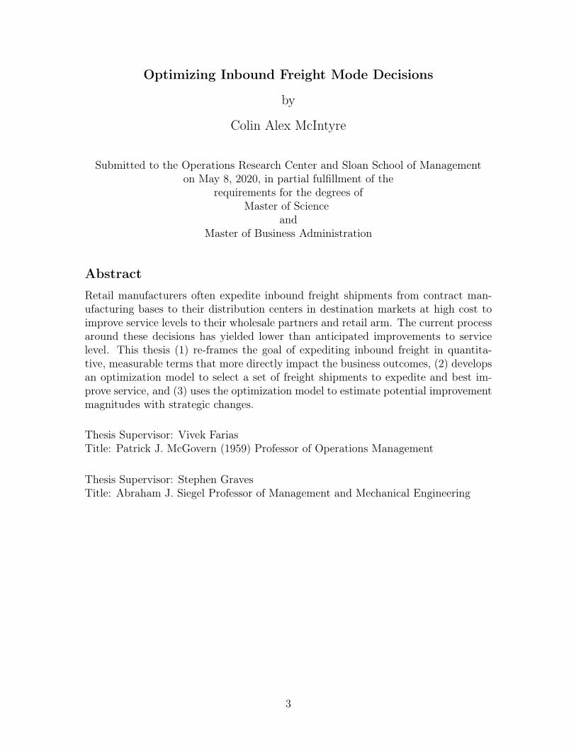
Retail manufacturers often expedite inbound freight shipments from contract man-ufacturing bases to their distribution centers in destination markets at high cost toimprove service levels to their wholesale partners and retail arm. The current processaround these decisions has yielded lower than anticipated improvements to servicelevel. This thesis (1) re-frames the goal of expediting inbound freight in quantita-tive, measurable terms that more directly impact the business outcomes, (2) developsan optimization model to select a set of freight shipments to expedite and best im-prove service, and (3) uses the optimization model to estimate potential improvementmagnitudes with strategic changes.

Thesis Supervisor: Vivek FariasTitle: Patrick J. McGovern (1959) Professor of Operations Management

Thesis Supervisor: Stephen GravesTitle: Abraham J. Siegel Professor of Management and Mechanical Engineering

3

4

Acknowledgments

I would like the thank the whole team at Nike for their warm welcome and integra-

tion into an incredibly talented and engaging team and culture. Gareth Olds and

Angharad Porteous were fantastic mentors, modelers, and proselytizers of analytics

to work with, and learn from. I thank them for the constant feedback that helped

me improve the work and the inclusion in runs, triathlons, commutes and trips that

integrated me so quickly into the team. I’d also like to thank the broader team of

stakeholders across the Advanced Analytics teams and the Global Operations Team

for all their help, specifically Jon Frommelt, Hugo Mora, Steve Sohn, Lauren Bronec,

Mario Wijaya, Liz Walker, John Jenkins, Nate De Jong, Hari Murakonda, Arun Jee-

vanantham, and Mark LeBoeuf.

From MIT, I am very grateful for the wonderful advice and support throughout

this thesis from Stephen Graves, Vivek Farias and Carolina Osorio. Their insight,

feedback, and guidance have been invaluable through this process and I appreciate

all their efforts.

To my friends across MIT and Boston and especially to my amazing classmates

at LGO, I am grateful for all your support through the internship and your warm

welcome back after almost a year away. It has been an absolute joy these last few

years and I am looking forward to seeing you thrive in life.

Finally to my parents, to Sean, and to Ariel: thank you for the love, guidance,

help, and fun during these last two years. I wouldn’t be here without all you’ve done

for me and I’m looking forward to many more great years.

5

Note on Nike Proprietary Information

To protect information that is proprietary to Nike, Inc., the data presented throughout

this thesis has been modified and does not represent actual values. Data labels have

been altered, converted or removed to protect competitive information, while still

conveying the findings of this project.

6

Contents

1 Introduction 13

1.1 Introduction to the Footwear and Apparel Industry . . . . . . . . . . 13

1.2 Company Overview . . . . . . . . . . . . . . . . . . . . . . . . . . . . 15

1.2.1 Nike’s Supply Chain Operations . . . . . . . . . . . . . . . . . 15

1.2.2 Current Nike Strategy . . . . . . . . . . . . . . . . . . . . . . 16

1.3 Problem Statement and Motivation . . . . . . . . . . . . . . . . . . . 18

1.4 Project Goals . . . . . . . . . . . . . . . . . . . . . . . . . . . . . . . 19

1.4.1 Introduction to Approach . . . . . . . . . . . . . . . . . . . . 19

2 Literature Review 23

2.1 The Air Freight Logistics Industry . . . . . . . . . . . . . . . . . . . . 23

2.2 Carbon Emissions and Business Context . . . . . . . . . . . . . . . . 24

2.3 Supply Chain Freight Optimization . . . . . . . . . . . . . . . . . . . 26

3 Objective Function Determination 29

3.1 Current State . . . . . . . . . . . . . . . . . . . . . . . . . . . . . . . 29

3.1.1 Purchase Orders . . . . . . . . . . . . . . . . . . . . . . . . . 29

3.1.2 Sales Orders . . . . . . . . . . . . . . . . . . . . . . . . . . . . 31

3.1.3 Relevant Metrics . . . . . . . . . . . . . . . . . . . . . . . . . 32

3.2 Existing Process . . . . . . . . . . . . . . . . . . . . . . . . . . . . . . 33

3.2.1 Process Outputs . . . . . . . . . . . . . . . . . . . . . . . . . 35

3.3 Proposed Changes . . . . . . . . . . . . . . . . . . . . . . . . . . . . 35

3.4 Use in Optimization and Communication . . . . . . . . . . . . . . . . 38

7

4 Formulation of Model 41

4.1 Mathematical Model Definition . . . . . . . . . . . . . . . . . . . . . 45

4.1.1 Decision Variables . . . . . . . . . . . . . . . . . . . . . . . . 45

4.1.2 Objective Function . . . . . . . . . . . . . . . . . . . . . . . . 46

4.1.3 Constraints . . . . . . . . . . . . . . . . . . . . . . . . . . . . 46

4.2 Sensitivities and Extensions . . . . . . . . . . . . . . . . . . . . . . . 50

4.2.1 Parameter Sensitivity Analysis . . . . . . . . . . . . . . . . . . 50

4.2.2 Forecasted Demand . . . . . . . . . . . . . . . . . . . . . . . . 51

5 Optimization Results 53

5.1 Analysis of Potential Improvement . . . . . . . . . . . . . . . . . . . 54

5.1.1 Implementing Improvements . . . . . . . . . . . . . . . . . . . 57

5.1.2 Solver Decisions and Model Solve Time . . . . . . . . . . . . . 59

5.2 Sensitivity Analyses . . . . . . . . . . . . . . . . . . . . . . . . . . . . 60

5.2.1 Fill Rate Sensitivity . . . . . . . . . . . . . . . . . . . . . . . 61

5.2.2 Discrete Mode Choice Relaxation . . . . . . . . . . . . . . . . 64

5.2.3 Deliver-to-need . . . . . . . . . . . . . . . . . . . . . . . . . . 64

5.3 Prioritization and Guidance on Implementation . . . . . . . . . . . . 65

6 Conclusions and Future Work 69

8

List of Figures

1-1 Simplified Sequence of Nike Supply Chain . . . . . . . . . . . . . . . 16

1-2 Simplified Network Model . . . . . . . . . . . . . . . . . . . . . . . . 20

3-1 Example Purchase Order . . . . . . . . . . . . . . . . . . . . . . . . . 30

3-2 Example Allocation Between Purchase and Sales Orders . . . . . . . 31

3-3 Simplified Supply Chain with Decision and Metrics Timing . . . . . . 32

3-4 Perishability and Relative Value by Category of Product . . . . . . . 37

4-1 Illustrative Diagram of Model. . . . . . . . . . . . . . . . . . . . . . . 42

4-2 Timeline of Key Dates and Lateness . . . . . . . . . . . . . . . . . . . 44

5-1 Budget and service level by scenario. . . . . . . . . . . . . . . . . . . 55

5-2 Value of service approximation . . . . . . . . . . . . . . . . . . . . . . 56

5-3 Typical Gurobi MIP Gap Pattern . . . . . . . . . . . . . . . . . . . . 60

5-4 Typical Gurobi Solution Pattern . . . . . . . . . . . . . . . . . . . . . 61

5-5 Pareto Frontiers with Different Fill Rate Constraints and Variable

Types for Shipment Decisions . . . . . . . . . . . . . . . . . . . . . . 63

5-6 Pareto Frontiers with Different Fill Rate Constraints and Variable

Types for Shipment Decisions Showing Improvement over Vessel Cases 63

5-7 Pareto Frontiers with Different Shipment Decision Variable Types Com-

pared to Current Operations . . . . . . . . . . . . . . . . . . . . . . . 65

5-8 Inbound Freight Carbon Contributions by Mode . . . . . . . . . . . . 66

5-9 Margin After Air Freight Including Carbon Costs . . . . . . . . . . . 68

9

10

List of Tables

3.1 Example of Tradeoffs to Calibrate Objective Values . . . . . . . . . . 40

5.1 Units by Shipment Mode and Lateness . . . . . . . . . . . . . . . . . 57

11

12

Chapter 1

Introduction

This thesis proposes and outlines a solution for improving decisions around inbound

freight mode selection. Many large companies rely on international shipping lanes

to bring products from their origin to customers around the world. Shipping lines,

air freight forwarders, rail companies, and trucking networks are some of the ma-

jor players all competing for this freight business, each providing a unique mode of

transport and value proposition to its segment of customers. This thesis details one

way of determining how to most efficiently send product through these various modes

to provide value for the large companies responsible for procuring and distributing

products.

1.1 Introduction to the Footwear and Apparel In-

dustry

The current landscape of footwear is dominated by athletics companies–Nike, Adi-

das, Puma, New Balance, Asics and others all earn billions of dollars of footwear

revenue each year. For some footwear companies, apparel has evolved to become a

co-equal pillar of the business. A simplified value stream for these four brands and

for Nike’s competitors in general (adidas, Puma, lululemon, VF, etc.) is a system

where products are produced by contract manufacturers around the world, sold to

13

these multinational brands (also called the ‘manufacturer’ throughout this thesis, as

opposed to ‘contract manufacturer’), shipped to higher-income countries, then dis-

tributed and sold through a combination of wholesale and internal direct-to-consumer

channels. As Phil Knight documented in his recent memoir, Nike was the first com-

pany to begin importing shoes from Asia to the US via a partnership with Onitsuka

Tiger in the 1960s, and for the most part, the industry followed suit.1 As it stands

now, the vast majority of product is made in low-cost countries around the world like

China, Vietnam, and Indonesia and transported to markets around the world. [9] [1].

The basic business model for manufacturers has shifted dramatically in the last

20 years. During the dot-com boom, Zappos, Amazon, and other direct-to-consumer

e-commerce platforms began to challenge the basic wholesaler business model of the

largest footwear and apparel brands [10]. Since the external innovations at the turn of

the millennium, the largest brands now operate their own physical and digital direct-

to-consumer platforms in addition to selling via dedicated e-commerce platforms like

Zappos, and through the e-commerce and brick-and-mortar channels of their whole-

sale partners. These changes have impacted the way consumers interact with brands,

with these large companies among the most eager to introduce omni-channel corpo-

rate strategy across supply chain, marketing, and endorsements. Where Nike and

Adidas once relied purely on athletes like Franz Beckenbauer, Michael Jordan, or

Billie Jean King to market their products, customers now interact with these brands

via influencers like Kanye West and high-profile Instagram users as well as Serena

Williams.

The flexibility and performance demanded from supply chains has increased dra-

matically due in part to the digital revolution reshaping consumer mindsets and

expectations. One social media post advertising a new shoe will drive demand all

across the world; different customers walking into a Nike store in Paris, a Foot Locker

in Kansas or opening their phone to the Nike app will all expect to be able to buy the

shoe that day. These demands require a fast, flexible, coordinated, and highly reliable

1Textile manufacturing takes place around the world with New Balance notably still maintaininga major US manufacturing base.

14

supply chain that is being created within these companies. Asking the supply chains

of twenty or even five years ago to fulfill that distributed demand in a coordinated

way would be impossible or astronomically expensive.

1.2 Company Overview

Nike, Inc. is the world’s largest footwear and apparel company with over $39 Billion

in revenue during the fiscal year ending May 2019. Nike, Inc. sells and distributes

its products under four brands–Nike, Jordan, Converse, and Hurley, the latter two

which operate as wholly-owned subsidiaries2.

Nike has expanded dramatically since its beginnings in the Pacific Northwest.

Today only 43% of its revenues come from North America, with the balance split

approximately equally across Europe, the Middle East, and Africa (EMEA); China,

Hong Kong, Macau, and Taiwan (Greater China); and Asia-Pacific and Latin America

(APLA) [12].

1.2.1 Nike’s Supply Chain Operations

Nike designers and researchers spend years developing technology and styles for future

apparel and footwear products, but Nike’s supply chain operations start months in ad-

vance of a sale and (returns notwithstanding) often end weeks prior to the end sale. In

the months leading up to a season, Nike solicits orders from wholesale customers and

develops internal predictions of demand. It orders product from contract manufac-

turers as Purchase Orders (POs), and as firm orders from its customers materialize,

commits to delivering a Sales Order (SO) to its customers. In Nike’s operations,

and in this thesis ‘customers’ refers to external wholesale partners (Dick’s Sporting

Goods, Nordstrom’s, Kohl’s, etc.) and to internal customers responsible for direct-

to-consumer channels, while ‘consumers’ refer to the individual actually purchasing

product in stores or online.

2Hurley was spun off from Nike in October 2019

15

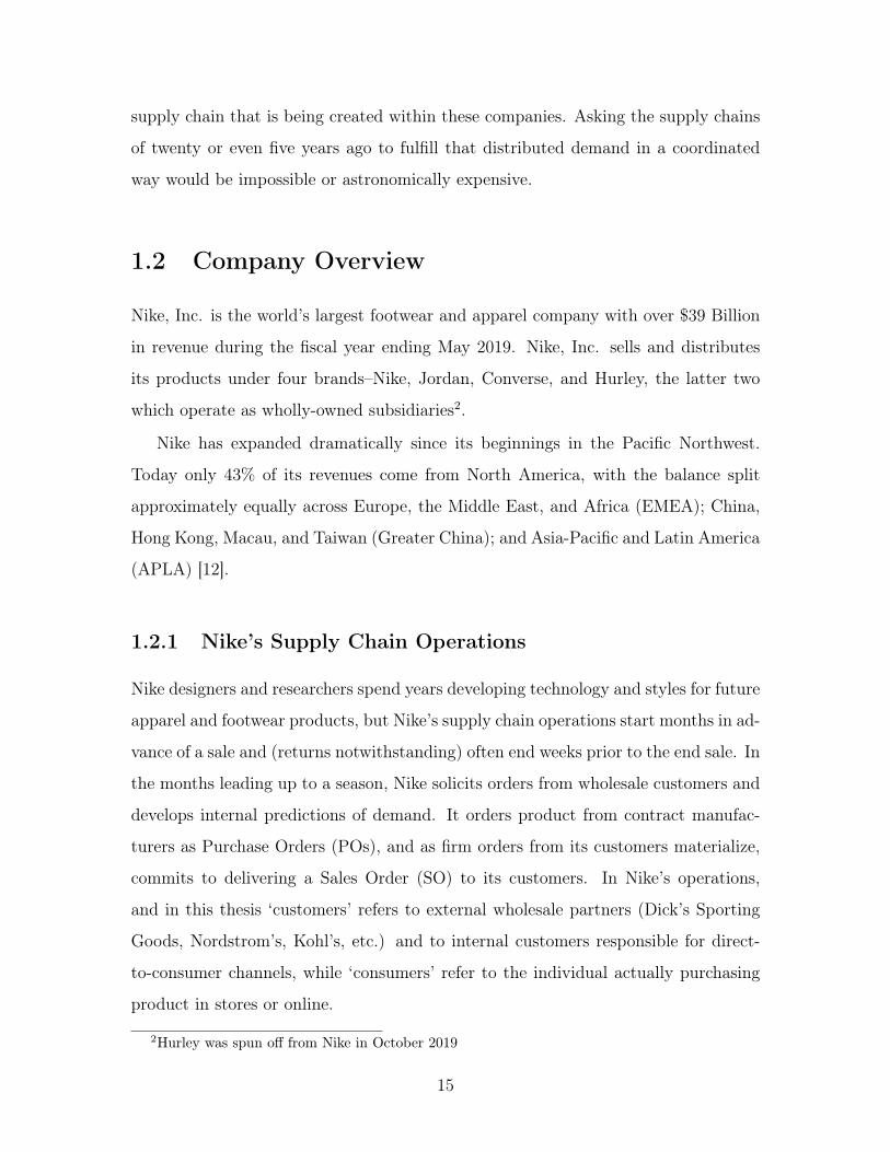
Figure 1-1: Simplified Sequence of Nike Supply Chain

In this thesis, we model the flow of inventory from the PO through the SO for

North America. This flow generally takes one of two forms: the product is shipped

directly to the customer’s distribution center, or the product is routed to one of

Nike’s 6+ distribution centers in the US, then on to the customer. The product flows

are split approximately 50/50 between these two channels for the North American

market. The thesis focuses primarily on product that flows through Nike’s DC for

reasons explained in Sec. 1.3.

In the vast majority of cases, the product will arrive at the departure port (in the

country where the product was manufactured, most often Asia) and be placed on a

ship to the US, arrive at port in the US where it clears customs and is placed on a truck

to Nike’s or to a customer’s DC. In some cases, Nike will elect to divert a PO from

the ship and instead fly product into the US, then truck it to the relevant distribution

center. If that PO flows through Nike’s DC, the product will be allocated to a SO

once it arrives at the distribution center. Once that SO is filled, all the product will

ship out to the customer. See Fig. 1-1 for an overview of the supply chain for product

routed via Nike’s DC.

1.2.2 Current Nike Strategy

Nike has always operated on the forefront of sport; to maintain that advantage, Nike

announced the Consumer Direct Offense in 2017. The Consumer Direct Offense sets

three ambitious goals known as the Triple Double: 2x Innovation, 2x Speed, and 2x

16

Direct to focus on innovative products; a fast and flexible supply chain; and emotional,

personal connections with consumers, respectively.[11] As discussed in Sec. 1.1, the

consumer landscape has changed to require the implementation of these ambitious

goals in order to reach these consumers wherever they are–online, in Nike’s brick-and-

mortar stores, or via wholesale partners. Nike’s biggest customers are facing similar

issues and demanding high levels of service from Nike in order to meet these changing

trends.

One lever to increase speed and flexibility is air freight. As diagrammed in Fig.

1-1, there is a choice of mode when product moves from consolidators in foreign ports

like Hanoi to domestic ports such as New York. Sea freight is preferable for its low

cost, and generally Nike’s supply chain can accommodate the long duration of trans-

Pacific sailings. The choice to switch a PO to air freight can be made to react to

outside factors, or to provide flexibility to Nike’s strategy. Outside factors include

demand fluctuations, factory delays, and material constraints generally outside Nike’s

direct control. Air freight may also be a strategic decision to better utilize factory

capacity or allow for longer design windows while still meeting agreed delivery dates.

Nike relies heavily on its largest customers to plan and execute its strategies and

to deliver its product to consumers. As such, Nike enters into agreements with its

customers to ship product only when Nike can fulfill all or almost all of the order

at once. For example, if a customer orders 10 units of product A and 20 units of

product B, Nike will not ship product A in one shipment and product B several

weeks later. The exact nature of these contracts are varied, time-dependent, and

complex, especially when paired with allocation logic discussed in previous theses

[8]. As such, it is difficult for a small group of people to manually make a decision

about expediting (for example) 1000 units of product A. Coordinating arrival several

weeks early to be able to say with confidence that more orders will be shipped to

customers due to that earlier arrival is difficult as delays to companion products may

delay outbound shipments.

17

1.3 Problem Statement and Motivation

The fundamental problem that this thesis addresses is the efficient utilization of re-

sources for inbound freight for product that flows through Nike’s North America

distribution centers. In order to activate the Consumer Direct Offense and increase

the speed of its supply chain, Nike needs to know that a dollar spent moving prod-

uct faster across the ocean will actually result in a customer getting that product

sooner than they would have otherwise. This responsiveness to customer demands

and efficient use of resources is crucial in a highly competitive retail market.

Shorter lead times throughout the supply chain can enable Nike to be closer to its

consumers by changing supply levels to meet uncertain demand, to better capitalize on

ethereal sports moments or brand heat events, and to bring new product innovations

to consumers more regularly. Some work in this space will more fundamentally alter

the supply chain, but there is an opportunity to make better decisions with the

same infrastructure by quantifying value and using analytic frameworks to better

understand the overall impact to the supply chain of individual decisions and drive

more holistically beneficial decisions.

This problem also presents an opportunity for Nike to better understand more

prescriptive analytics and its impact on internal company processes and supply chain

outcomes. As such, this work focuses on the subset of Nike orders that flow through

internal distribution centers. By focusing internally, Nike can have more control over

implementation and performance measurement in the short term. In the long term,

Nike views engagement with wholesale partners and smaller customers as crucial to

its long term success, and performance improvement across its network of suppliers,

internal business units, and customers will require spreading mechanisms for making

better, more consistent decisions. This means that a natural extension of this work

is understanding the relevant changes required to adapt these decisions to benefit the

entire network.

18

1.4 Project Goals

The major contribution to Nike’s business process is a new model which evaluates the

current state of the supply chain and order book and recommends decisions about

the right set of products to expedite via air freight to improve customer outcomes.

The model will take as inputs the current state of Nike’s orders and quantified values

representing the priorities Nike places on certain products; the development of these

inputs is discussed further. The model will then solve for efficient outcomes which

are possible subject to supply chain parameters like travel and processing times and

Nike’s constraints like available budget and procured air freight capacity. The goal

of this model is not to recommend one scenario that produces the best outcome,

but instead several different possibilities with tradeoffs between cost of service and

quality of results. Understanding these tradeoffs will allow for a strategic decision

about improving service levels or reducing costs.

Producing this new model will also require establishing a quantitative way to eval-

uate the outcomes of air freighting. This thesis also explores the quantification of the

current business practices surrounding the air freight decisions and the establishment

of a measurement of the benefits of air freight in addition to the costs. We measure

the benefits of the current state and show how the model can be used to provide

higher outcomes at lower cost.

1.4.1 Introduction to Approach

To provide relevant context to the methods, a summary of the approach is presented

here, with more detailed discussion throughout the thesis.

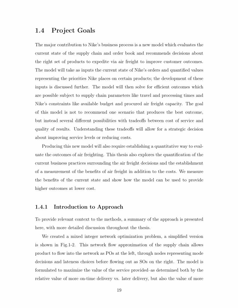
We created a mixed integer network optimization problem, a simplified version

is shown in Fig.1-2. This network flow approximation of the supply chain allows

product to flow into the network as POs at the left, through nodes representing mode

decisions and lateness choices before flowing out as SOs on the right. The model is

formulated to maximize the value of the service provided–as determined both by the

relative value of more on-time delivery vs. later delivery, but also the value of more

19

Figure 1-2: Simplified Network Model

important products. Key constraints assessed on the model include:

∙ Budget: as determined by the volume of product using a specific node

∙ Lane Capacity: certain transportation lanes have volume limits

∙ Timing: linking only the nodes corresponding to a feasible arrival date given

the inbound mode and the shipment date required by the SO

∙ Allocation: linking product from a certain PO to a certain SO given the most

recently available allocation forecast.

To determine the best possible options, we run the model with different budgets

and maximize service in each case to see the tradeoffs between cost and service, and

run useful sensitivity analyses to model the impact on these transportation decisions.

The rest of this thesis walks through the achievement of these goals with the

following structure

1. Chapter 2 describes relevant optimization, supply chain, and transportation

modeling, and how this work contributes to the literature

2. Chapter 3 evaluates the current business processes and a new proposal for eval-

uative metrics to improve the inbound freight process

20

3. Chapter 4 lays out the mathematical framework of the network optimization

problem and how the modeling choices I made best represent business realities

4. Chapter 5 presents the results of the optimization model and several different

scenarios for improving performance with specific customer classes

5. Chapter 6 discusses the recommendations and implementation strategies rele-

vant to the model and its results

21

22

Chapter 2

Literature Review

Supply chain management has leveraged optimization for decades, especially over the

last several years as optimizations algorithms and computing power have caught up

with the scale and complexity of global supply networks. In my review of the relevant

literature, I find that the basic principles leveraged in this thesis have been used time

and again in adjacent questions, but low-level decision making such as freight mode

choice for each order has not leveraged these tools. Due to the market dynamics and

impact of the air freight decisions, it will be important to make good decisions about

the use of air freight in the future. This section explores the industry, its dynamics,

and the importance of air freight decisions in the near future.

2.1 The Air Freight Logistics Industry

The state of the global air freight market suggests that this is a key area to invest

in better decision making. While the total cost of logistics in the United States

has hovered around 8% consistently for the last decade [13], the air freight industry

is forecasted to continue to grow approximately 4% annually over the next 20 years,

growing 10% year-over-year as recently as 2017 [5]. Air cargo transportation accounts

for less than 1% of total trade by volume while transporting over 35% of global trade

by value. In order to compete with such high-value goods in the transportation

network, retailers with lower input costs and value-to-volume ratios will need to be

23

exacting in their use of air freight or else risk paying premiums to compete with

high value products. The air cargo industry’s frequent fliers: consumer electronics,

flowers, fresh fish, and specialized equipment can all justify air freight premiums due

to infeasible alternatives or inventory holding costs, while traditional textile retailers

look at this premium as a potential saving if slower, cheaper modes are suitable for

market needs.

Despite the premium on air freight and the explosive growth of the industry,

textiles have actually been increasing their market share in the key lane from East

Asia in to North America [5]. Between 2016 and 2017, apparel’s market share grew

14% over the year to represent 15% of the total tonnage between the two regions.

The air freight industry between East Asia and North America has been dominated

by China-US trading of late. Chinese exports now represent approximately half of all

East Asian air freight exports by weight, up from 14% twenty years ago. The Chinese

growth corresponded to a shirking of Japanese exports over the same time frame, and

now seems to be threatened by a booming Vietnamese economy as textile, footwear,

electronics, and machinery manufacturers look for cheaper labor outside China and

seek political stability and supply base diversification.

This theme is replicated across other regions as well. In both East Asia-Europe

and intra-East Asian air freight trade, China has grown to become the dominant

power in the region while the growth in peripheral economies threatens to reduce

Chinese market share, if not their gross freight value or volume.

2.2 Carbon Emissions and Business Context

Climate change is the single most impactful issue for humanity today and likely

will be for the foreseeable future. A recent UN report forecasted mass extinctions,

rising sea levels, and widespread famine, droughts, and poverty within in the next 20

years if humanity continues to pollute the atmosphere with greenhouse gasses [14].

A 2014 report by the UN attributed 15% of global greenhouse gas emissions to the

transportation sector, the fourth largest group behind electricity and heating, farming

24

and agriculture, and industrials.

With nonexistent political leadership on climate change in the United States,

corporations have begun to impose goals on themselves above and beyond standards

imposed by the government in areas like emissions, labor sustainability, and overall

environmental impact. This change is a notable departure from policies of just 20

years ago and is due to many factors. In 1998, a group of petroleum majors spent

millions of dollars lobbying against US ratification of the Kyoto Protocol as part of a

general strategy to make regulations favorable to major emitters of carbon [6]. Now,

Chevron publically advertises its climate change initiatives–though its core business

model has not materially changed [4]. Experts cite many reasons for these shifts, not

least of which being the mountain of scientific evidence, but consumer perceptions of

brands, customer choice in the market, and a dearth of political will are all cited as

factors [17].

As companies look to reduce their environmental impact and improve the public

perception of their sustainability, the supply chain is a natural first place to look. As

mentioned, transportation is a major source of carbon emissions. The transportation

mode as well as the distance travelled are the two main factors impacting the scale

of carbon emissions for moving a given product from source to consumer. The World

Shipping Council estimates that the carbon impact per weight and distance travelled

is over 100x higher for air freight than ocean freighter and over 5x higher than heavy-

duty truck [15]. In comparing ocean freight to air freight in intercontinental shipping,

ancillary over-land routes taken my rail, inland waterway, or truck may change the

exact factor by which air freight generates more carbon, but the order of magnitude

of air freight emissions means that any air-based route will substantially out-emit any

sea-based route.

Despite the outsize per-unit air freight carbon impact, ocean freight is estimated

to be responsible for some 2% of global carbon emissions [15]. In the early 2010s large

ocean freight vessels begun ‘slow-steaming’ in an effort to curb rising fuel costs and

save fuel over the course of the journey by reducing speed [19]. This has the added

benefit of reducing emissions from ocean freight, but causes capacity constraints,

25

longer lead times, and increased inventory costs due to the increase in time ships take

to sail across the ocean. This practice has mostly reversed in the years since oil prices

spiked, and environmental groups have advocated a regulatory approach to reducing

speed. The current climbing oil prices may bring back the practice on fuel economics

alone [18].

2.3 Supply Chain Freight Optimization

Bravo and Vidal establish a review of freight transportation modeling in supply chain

optimization models and find several trends both in the last few years and over the

last decades [2]. First, they find that researchers favor an integrated optimization

approach over a hierarchical one. Much of the literature around freight optimization

also takes the size, location, and function of supply chain network nodes as variables.

In cases where these factors are co-optimized with freight considerations, results are

superior to a staged approach where the network is set then freight decisions are

made.

Combining both the network design and operational decisions is not entirely

straightforward. Cardona-Valdes et.al. formulates a bi-objective problem where the

network design problem is formulated as a combinatorial assignment of plants 𝐼 to

locations 𝐽 and serving customers 𝐾 via those paths at some location and mode-

dependent cost [3]. The use of a bi-objective framework has the feature of not identi-

fying one particular optimal solution but instead outlining a pareto frontier of optimal

solutions given different weights to the two objective functions–in this case cost of

the network and time required to deliver to customers. A drawback of the pareto

frontier is that the methods do not provide direction on where on the frontier would

be best to operate–that comes from the business realities surrounding the problem.

In practice, a sharp transition in the shape of the pareto frontier may suggest a highly

sensible operation point.

While this bi-objective approach was preferred to a purely sequential optimiza-

tion, there was a trend in the papers reviewed by Bravo and Vidal of using cost

26

minimization as the objective function for the vast majority of problems. In imple-

menting optimization, cost minimization has the obvious advantage that the solution

provided will cost less than any other feasible set and is therefore palatable to business

users. It is also the most easily quantified parameter of the supply chain. It is perhaps

no surprise that the business function often viewed as a cost center is ubiquitously

modeled as a cost to minimize in the academic literature.

One work that attempted to move away from a purely cost based view of supply

chain optimization was Paksoy et. al. [16]. The paper is in some way a prototypical

supply chain cost optimization to minimize costs by directing product from man-

ufacturers through distributors to retailers given different costs of each path. They

introduced a layer of complexity by making the quality of the products a decision vari-

able and introducing a probability of rework to penalize low quality. This approach

struggles to correspond to a complex evaluation of the tradeoffs of just-in-time, e-

commerce, or large retail supply chains, but instead is an interesting extension of

Juran’s optimal quality tradeoff as applied to network optimization. The concept is

feasible if cost and quality are as inexorably linked as to provide a exhaustive ex-

planation of the value of the supply chain. However, other factors like timeliness,

completeness of order, and historical service levels will impact the value customers

receive from a high-functioning supply chain and are difficult to capture in one metric

of quality, and the average rework required given a level of quality.

The framework that this thesis follows can be seen in Diabat and Simchi-Levi’s

paper exploring shipping choice in a carbon-constrained world [7]. The problem

is a supply chain network optimization involving the choice of distribution center

locations and customers to serve from each location, subject to a constraint on the

amount of carbon that can be emitted transporting the goods from each DC to all

customers. The objective function used to position the DCs and allocate shipping

lanes minimized the cost of the total network subject to a total carbon emissions

constraint. Various scenarios with different carbon constraints then sketched out

a pareto frontier showing the tradeoffs between minimal supply chain cost and the

carbon emissions of the network. Assuming that there is generally some cost benefit

27

to increasing carbon emissions, this pareto frontier shows the tradeoff of reducing

carbon emissions and reducing costs through the supply chain.

28

Chapter 3

Objective Function Determination

Key to developing and communicating an optimization framework for decision mak-

ing is understanding the business goal the model will improve and translating it to

a mathematical formulation. Related analyses have shown that a high proportion of

the goods air freighted to market were not shipped out of distribution centers quickly

and the outbound shipment dates could likely have been met by using slower inbound

modes. The analyses also found that an important factor in these goods remaining

stagnant in the DCs was due to incomplete orders: high importance goods were or-

dered on the same order as lower importance goods, and all units need to be available

in order for the order to ship out.

Below, I lay out the current metrics used to track inbound freight results, their

shortcomings, and the business processes surrounding the air freight decision. I then

propose a service-level maximization objective function subject to budget constraints

and motivation for that decision.

3.1 Current State

3.1.1 Purchase Orders

Purchase Orders (POs) are the unit of supply to the manufacturer and the unit of

communication between the manufacturer (brand) and a given contract manufacturer.

29

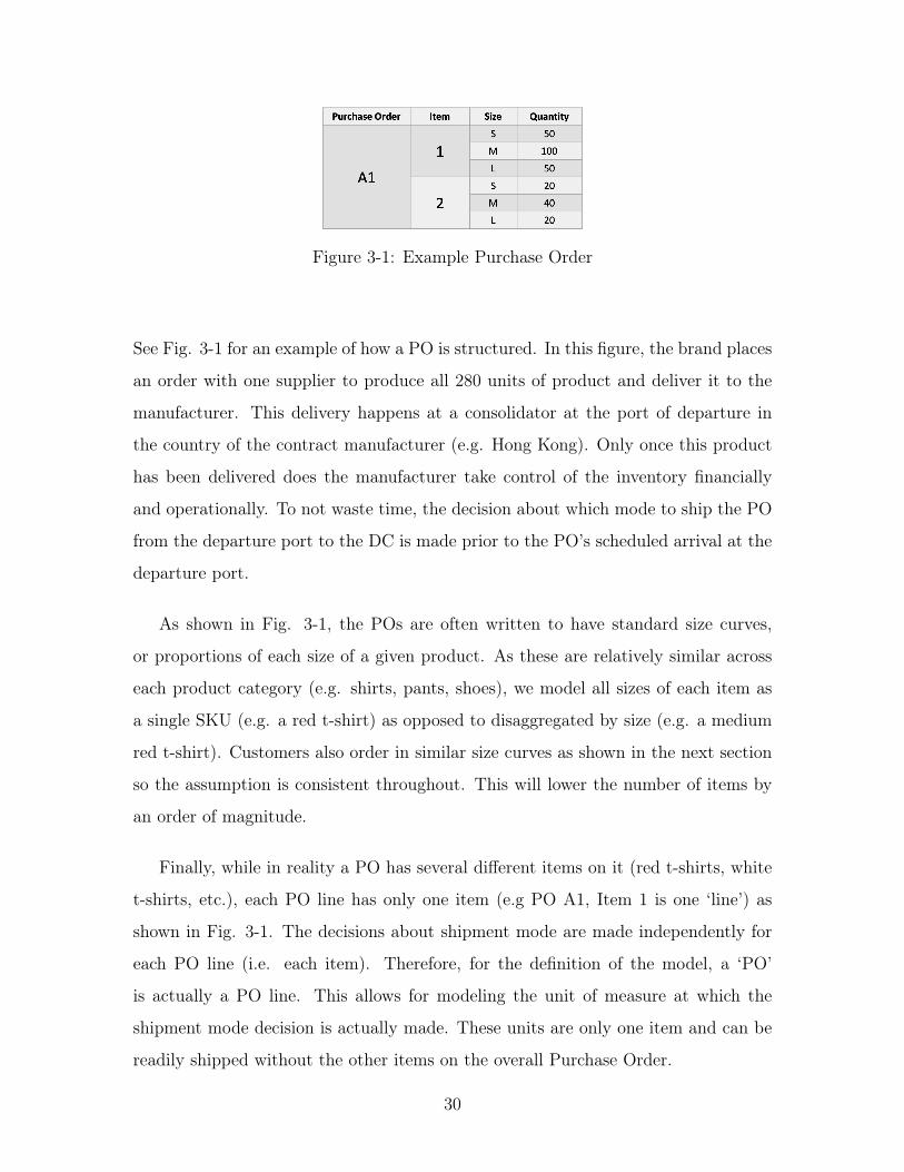
Figure 3-1: Example Purchase Order

See Fig. 3-1 for an example of how a PO is structured. In this figure, the brand places

an order with one supplier to produce all 280 units of product and deliver it to the

manufacturer. This delivery happens at a consolidator at the port of departure in

the country of the contract manufacturer (e.g. Hong Kong). Only once this product

has been delivered does the manufacturer take control of the inventory financially

and operationally. To not waste time, the decision about which mode to ship the PO

from the departure port to the DC is made prior to the PO’s scheduled arrival at the

departure port.

As shown in Fig. 3-1, the POs are often written to have standard size curves,

or proportions of each size of a given product. As these are relatively similar across

each product category (e.g. shirts, pants, shoes), we model all sizes of each item as

a single SKU (e.g. a red t-shirt) as opposed to disaggregated by size (e.g. a medium

red t-shirt). Customers also order in similar size curves as shown in the next section

so the assumption is consistent throughout. This will lower the number of items by

an order of magnitude.

Finally, while in reality a PO has several different items on it (red t-shirts, white

t-shirts, etc.), each PO line has only one item (e.g PO A1, Item 1 is one ‘line’) as

shown in Fig. 3-1. The decisions about shipment mode are made independently for

each PO line (i.e. each item). Therefore, for the definition of the model, a ‘PO’

is actually a PO line. This allows for modeling the unit of measure at which the

shipment mode decision is actually made. These units are only one item and can be

readily shipped without the other items on the overall Purchase Order.

30

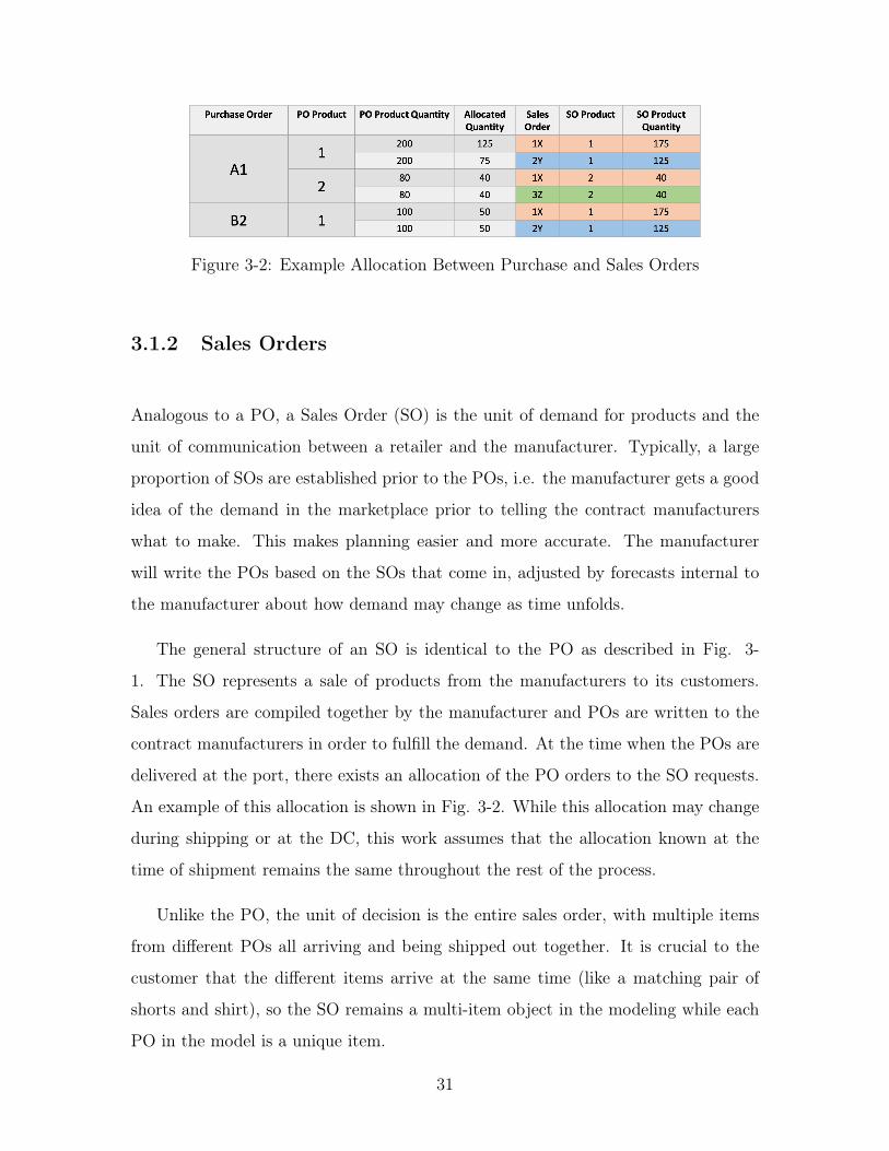
Figure 3-2: Example Allocation Between Purchase and Sales Orders

3.1.2 Sales Orders

Analogous to a PO, a Sales Order (SO) is the unit of demand for products and the

unit of communication between a retailer and the manufacturer. Typically, a large

proportion of SOs are established prior to the POs, i.e. the manufacturer gets a good

idea of the demand in the marketplace prior to telling the contract manufacturers

what to make. This makes planning easier and more accurate. The manufacturer

will write the POs based on the SOs that come in, adjusted by forecasts internal to

the manufacturer about how demand may change as time unfolds.

The general structure of an SO is identical to the PO as described in Fig. 3-

1. The SO represents a sale of products from the manufacturers to its customers.

Sales orders are compiled together by the manufacturer and POs are written to the

contract manufacturers in order to fulfill the demand. At the time when the POs are

delivered at the port, there exists an allocation of the PO orders to the SO requests.

An example of this allocation is shown in Fig. 3-2. While this allocation may change

during shipping or at the DC, this work assumes that the allocation known at the

time of shipment remains the same throughout the rest of the process.

Unlike the PO, the unit of decision is the entire sales order, with multiple items

from different POs all arriving and being shipped out together. It is crucial to the

customer that the different items arrive at the same time (like a matching pair of

shorts and shirt), so the SO remains a multi-item object in the modeling while each

PO in the model is a unique item.

31

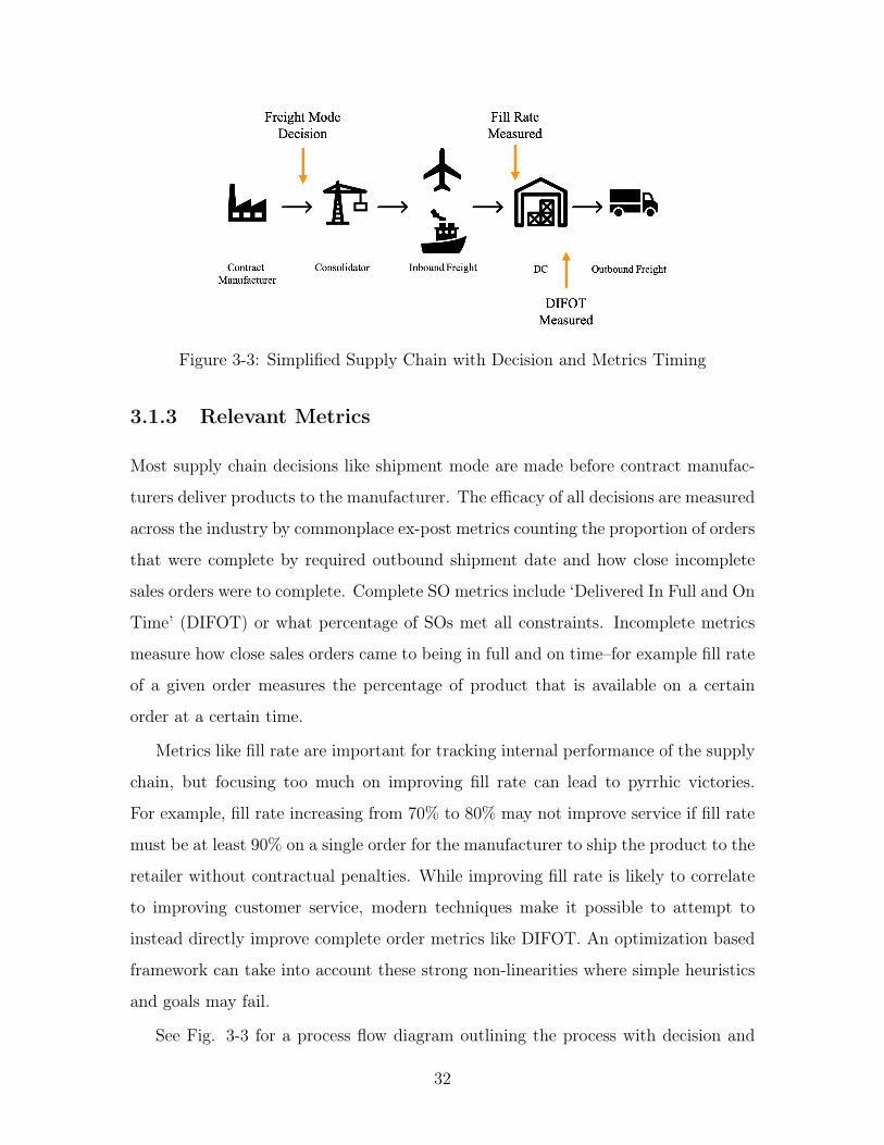
Figure 3-3: Simplified Supply Chain with Decision and Metrics Timing

3.1.3 Relevant Metrics

Most supply chain decisions like shipment mode are made before contract manufac-

turers deliver products to the manufacturer. The efficacy of all decisions are measured

across the industry by commonplace ex-post metrics counting the proportion of orders

that were complete by required outbound shipment date and how close incomplete

sales orders were to complete. Complete SO metrics include ‘Delivered In Full and On

Time’ (DIFOT) or what percentage of SOs met all constraints. Incomplete metrics

measure how close sales orders came to being in full and on time–for example fill rate

of a given order measures the percentage of product that is available on a certain

order at a certain time.

Metrics like fill rate are important for tracking internal performance of the supply

chain, but focusing too much on improving fill rate can lead to pyrrhic victories.

For example, fill rate increasing from 70% to 80% may not improve service if fill rate

must be at least 90% on a single order for the manufacturer to ship the product to the

retailer without contractual penalties. While improving fill rate is likely to correlate

to improving customer service, modern techniques make it possible to attempt to

instead directly improve complete order metrics like DIFOT. An optimization based

framework can take into account these strong non-linearities where simple heuristics

and goals may fail.

See Fig. 3-3 for a process flow diagram outlining the process with decision and

32

metric measurement timing within it. Crucially, fill rate is a metric internal to the

distribution center, but DIFOT measures the outbound performance of the DC, which

the customer will also see.

For our task specifically, any expedited order will improve the fill rate by increasing

the fill rate at time 𝑡 or by making the order full at 𝑡′ < 𝑡 or both. However, this

may not improve the DIFOT metric as expediting late product may not be sufficient

to trigger the shipment conditions to have the product ship earlier. The non-linear

relationship between expediting and DIFOT improvement is precisely what makes

optimization algorithms an attractive link between data and improved outcomes.

Highly manual decision processes are bound to target more linear relationships like fill

rate as opposed to non-linear metrics like DIFOT. Regardless of the metric targeted

for improvement, the modeling has fundamental information constraints, discussed

below.

A key previous analysis attempted to identify the ex-post effectiveness of expe-

diting an order by building an counterfactual inventory position if the order had not

been expedited. If the actual shipments of the product would have caused the distri-

bution center to stock out in the counterfactual world, then the shipment is labeled

‘effective’. This analysis showed that a large portion of the expedited items were

ineffective–largely due to expedited products sitting in the distribution center wait-

ing for other products to arrive and the shipment to fill up to an adequate level to be

shipped.

3.2 Existing Process

Currently, each month planners sit down with account managers and evaluate the

current state of the supply chain and the expected service levels. Where service levels

are unsatisfactory (for example, product class A for customer X is on average trending

late for 50% of sales orders), products from the given product class will be expedited

on SOs that are allocated to that customer. There is a budget target for all expediting

across all customers, and the most strategically important customers hold the most

33

sway.

Due to the transit times available from shipping providers, the decision of freight

mode choice takes place before relevant data may be available. Decisions about freight

mode are made up to a month before the order arrives at the departure port, and

over two months before the estimated arrival time at the onshore distribution center

(assuming product is shipped by vessel). During these two months, several important

factors can change or become known (such as actual consumer demand), so many

decisions are made with limited data.

Current processes heavily weight the input of customers, as they have a crucial

consumer-facing perspective of what types of products (materials, colors, or styles)

are selling well at full price from different manufacturers. The input from these

customers does not take into account tradeoffs between customers or the overall cost

of the system, so costs increase easily without a full understanding of what expedited

shipments will truly add value to the customers writ large.

The advantages of the highly manual system include an understanding of customer

needs for expedited supply and the root causes of those needs, be it imminent unmet

demand, a promotion, or key products for internal marketing. People understand

better than a machine what the end customers want to feel from their manufacturers

and how those needs have been met in the past. With that in mind, we set out to

develop a method that would leverage the prioritization and customer service intuition

developed from a largely manual process and incorporate modern analytics to better

meet the targets the process is already striving towards.

Finally, the current business process has variable budgets depending on the avail-

able resources and the nature of the supply chain service levels. Therefore, the initial

budget decisions about air freight spend are to be made in a separate environment

from the tactical decisions of which POs to expedite. With that in mind, the proposed

approach will allow for the most important decisions to be prioritized regardless of

the budget.

The stakeholders in this process were not dissatisfied with several of the fundamen-

tals of the process–a monthly review time seemed satisfactory, the level of engagement

34

was good, and parties understand that this process can be improved either by lower-

ing costs, increasing effectiveness, or both. The stakeholder process to determine an

effective way to augment this decision with analytics explored many options, and the

most effective is summarized below.

3.2.1 Process Outputs

This consultative stakeholder process ends with a determination of the shipping mode

for each PO. As discussed, this decision is made for each item separately, allowing

for red t-shirts to be air freighted and white t-shirts to go by sea, even if they were

ordered from the contract manufacturer together and we refer to each item on its own

as a PO.

This mode choice can result in product being shipped by air, by sea, or by a new

combination mode called sea-air where it is ocean shipped to a different port then

air freighted the remainder of the way–generally at a slightly lower cost to basic air

freight. Mimicking this output is the chief actionable decision of the model. These

decisions go to the consolidators who follow the instructions about how to ship the

product, and also to internal transportation teams who work to secure the specific

capacity necessary. This portion of the process remains largely unchanged but will be

working with different decisions after the implementation of the optimization model.

3.3 Proposed Changes

This optimization model will fit into a business decision process that is mostly un-

changed. The decisions will still take place approximately monthly, and during that

process, the shipment modes will be decided for the orders that are arriving at de-

parture ports in the next month. This means that the model will not have to run

particularly quickly, but will need to fit into the current workflow well and be flexible.

The model will use an objective function that will maximize service levels subject

to a budget constraint, with service levels defined below but crucially shifting the

measure from inbound service to outbound service (i.e. no reward for air freighting a

35

product into a DC, only a reward for shipping it out of the DC).

There are several other options for evaluating efficiency of production that we did

not pursue. One straightforward option is to evaluate the costs and benefits of the

target decisions in the same units (often currency), and maximize the profits subject

to constraints. While this would be a clean way to determine the best outcome, it

is not the method we chose primarily due to the difficulty generating a currency-

based metric that accurately represents service levels. Not only is an estimate of

revenue or profit based on when a product is delivered to a customer very uncertain,

the retail space has many other factors influencing how much more valuable a given

product is on time than it would be if it were late. The amount of marketing spent

for the product from the selling brand or the point-of-sale retailer, the availability

of substitutes, presence of other brands, presentation of the product with a suite of

complements, and the relationship history between the wholesaler and retailer all

factor in to the value of on-time delivery of a certain product. Fully incorporating all

of these factors into an accurate dollar impact, let alone dollar impact per unit was

not feasible. Given the uncertainty of such a measure, it would not combine well with

the relative certainty of the financial costs of the network for a single unit. Instead,

we focused on a non-financial measure of value for each product, and maximized that

value subject to a cost constraint on financial expense.

These confounding factors suggested leveraging the human intuition surrounding

the decision processes, as the end business objective is customer satisfaction at rea-

sonable cost and the people involved in the decision have years of experience. The

goal then is to standardize and quantify the intuition so that the best decisions can

be scaled across the entire set of orders.

During several workshops with the stakeholders, we developed metrics to quantify

the tradeoffs between different categories of goods and different lateness of delivery.

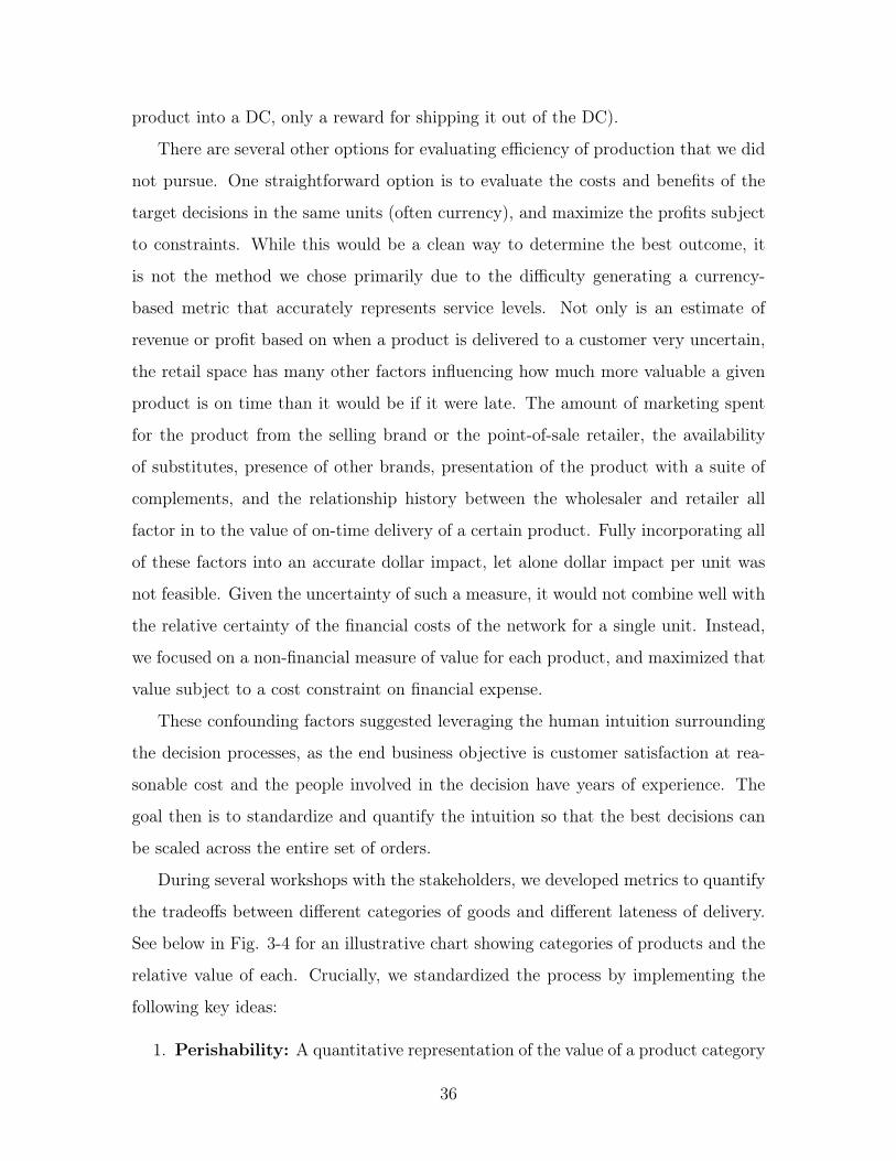
See below in Fig. 3-4 for an illustrative chart showing categories of products and the

relative value of each. Crucially, we standardized the process by implementing the

following key ideas:

1. Perishability: A quantitative representation of the value of a product category

36

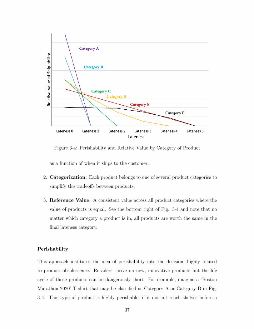
Figure 3-4: Perishability and Relative Value by Category of Product

as a function of when it ships to the customer.

2. Categorization: Each product belongs to one of several product categories to

simplify the tradeoffs between products.

3. Reference Value: A consistent value across all product categories where the

value of products is equal. See the bottom right of Fig. 3-4 and note that no

matter which category a product is in, all products are worth the same in the

final lateness category.

Perishability

This approach institutes the idea of perishability into the decision, highly related

to product obsolescence. Retailers thrive on new, innovative products but the life

cycle of those products can be dangerously short. For example, imagine a ‘Boston

Marathon 2020’ T-shirt that may be classified as Category A or Category B in Fig.

3-4. This type of product is highly perishable, if it doesn’t reach shelves before a

37

very short window (often minutes or hours for some product), it is worthless. This

life cycle is important to note because it could be the case that product could be

expedited to make it less late, but not to make it within a window of value. These

lost causes may as well be placed on a ship, given they will have to be sold at a

discount or loss anyway. Conversely, a simple black pair of shorts may be in season

for months or years, and lateness has less of an impact on the value of that product.

Only once contractual charges come into effect does lateness severely impact the value

to the manufacturer.

Reference Value

The tradeoffs between different category perishability begins with an equal starting

point. In the case of Fig. 3-4, each unit of product is worth the same if it is delivered

during Lateness 5. While this is not a reasonable assumption on its face given the

difference between the value of a high end pair of shoes and a pair of socks, it is a

reasonable approximation of the profits on the sale. If customers cancel or return

very late product, a reasonable assumption is that the manufacturer recovers its cost

by selling the product at cost through discount channels. The value of each category

can then be compared to this reference value when product is in lateness category 5.

As explained above, this ’at-cost’ worthlessness can be true for much earlier delivery

categories for more perishable product (see product categories A and B immediately

becoming worthless).

3.4 Use in Optimization and Communication

This classification and quantification feed directly into the objective function for the

optimization problem. The exact formulation is described in Sec. 4.1, and follows the

idea that a product of a given category arriving at a given lateness will have value as

shown in Fig. 3-4. The model has the ability to improve this objective function by

deciding to ship product by faster modes to arrive during better lateness times. This

will incur higher costs, so the model must choose to expedite the units that will most

38

cheaply improve the total value.

Two specific improvements that can be seen purely from this formulation are

the abandonment of lost causes and optimal tradeoffs. First, imagine a product in

Category A which will arrive in Lateness 5 via the slowest (and cheapest) shipping

mode and will arrive in Lateness 1 via the fastest (and most expensive) mode. In this

case, the framework will show that both outcomes are equally bad, with arrival at

Lateness 1 costing much more. Second, in a case where two products are both arriving

in Lateness 2, where one is Category C and another is Category A, expediting both

products to arrive in Lateness 0 will set up a scenario where the increase in value due

to the Category A unit is twice the increase of the Category C unit. If the Category

C unit can be expedited for less than half the cost of the Category A unit, then the

model will choose to ship two Category C units over one Category A unit. In general,

products have remarkably similar shipping costs, so Category A will be prioritized

over Category C.

One way that was effective in communicating the concept of relative value and

confirming the relative values of each category is to look at the implied values of

one ‘point’ given the approximate margin of each category. See Table 3.1 for a table

showing an example of the decrease in value of each category if it moves from Lateness

0 to Lateness 1. Using approximate data on the margin earned by a product in each

category, we can use the difference between the value attributed to each category

between Lateness 0 and Lateness 1 to calculate the implied probability of cancellation,

and ensure that the results approximate reality. For example, we can see that our

customers would behave similarly with respect to Category A or Category B products

being Lateness 1 or greater–they would immediately cancel the order. The value to

the manufacturer is different between the categories because of the margin difference,

not the a difference in the customer’s behavior. A contrasting pattern can be seen

by comparing Categories C and D, where the margin earned by the manufacturer on

each product is similar, but a higher value is assigned to Category C being Lateness

0 over Lateness 1 than is assigned to Category D. This would then imply that though

the manufacturer is indifferent between either product selling, due to the retailers

39

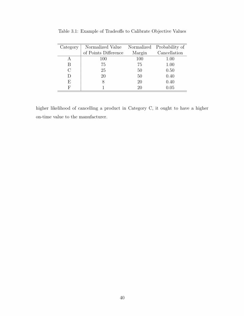
Table 3.1: Example of Tradeoffs to Calibrate Objective Values

Category Normalized Value Normalized Probability ofof Points Difference Margin Cancellation

A 100 100 1.00B 75 75 1.00C 25 50 0.50D 20 50 0.40E 8 20 0.40F 1 20 0.05

higher likelihood of cancelling a product in Category C, it ought to have a higher

on-time value to the manufacturer.

40

Chapter 4

Formulation of Model

The mathematical formulation of our model is a tiered network flow model where

the flows between nodes represent product, and each product must flow through four

tiers listed below. For mathematical notation, the four tiers are indexed by 𝑖, 𝑗, 𝑘,

and 𝑙, respectively.

1. The Purchase Order Tier: One node for each purchase order

2. The Mode Tier: For each purchase order, one node per viable shipment mode

3. The Lateness Tier: For each sales order, one node per viable lateness of that

order

4. The Sales Order Tier: One node for each sales order

Product flows through exactly one node in each tier from purchase to sales or-

der through one each of three types of edges on the network, labeled 𝛼, 𝛽, and 𝛾,

respectively. These are discussed more in Sec. 4.1.1

1. 𝛼𝑖,𝑗 the flow from PO tier node 𝑖 to mode tier node 𝑗

2. 𝛽𝑗,𝑘 the flow from mode tier node 𝑗 to lateness tier node 𝑘

3. 𝛾𝑘,𝑙 the flow from lateness tier node 𝑘 to SO tier node 𝑙

41

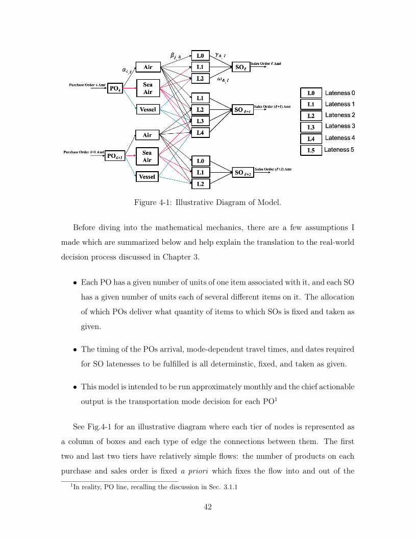
Figure 4-1: Illustrative Diagram of Model.

Before diving into the mathematical mechanics, there are a few assumptions I

made which are summarized below and help explain the translation to the real-world

decision process discussed in Chapter 3.

∙ Each PO has a given number of units of one item associated with it, and each SO

has a given number of units each of several different items on it. The allocation

of which POs deliver what quantity of items to which SOs is fixed and taken as

given.

∙ The timing of the POs arrival, mode-dependent travel times, and dates required

for SO latenesses to be fulfilled is all determinstic, fixed, and taken as given.

∙ This model is intended to be run approximately monthly and the chief actionable

output is the transportation mode decision for each PO1

See Fig.4-1 for an illustrative diagram where each tier of nodes is represented as

a column of boxes and each type of edge the connections between them. The first

two and last two tiers have relatively simple flows: the number of products on each

purchase and sales order is fixed a priori which fixes the flow into and out of the

1In reality, PO line, recalling the discussion in Sec. 3.1.1

42

system. The flows from each purchase order to its associated mode tier nodes is

allowed (and no flows to any other purchase order’s mode tier nodes are allowed).

Similarly, each lateness tier node has a connection to only one sales order node. The

connections between the mode tier and lateness tier nodes are more complicated. The

allocation between a PO and an SO is fixed a priori and a connection is established

between a given mode node and lateness node if and only if product is allocated from

the PO associated with the mode to the SO associated with the lateness and the

timing of shipping that PO via the associated mode will allow for delivery to the SO

at the specified lateness.

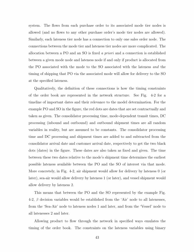
Qualitatively, the definition of these connections is how the timing constraints

of the order book are represented in the network structure. See Fig. 4-2 for a

timeline of important dates and their relevance to the model determination. For the

example PO and SO in the figure, the red dots are dates that are set contractually and

taken as given. The consolidator processing time, mode-dependent transit times, DC

processing (inbound and outbound) and outbound shipment times are all random

variables in reality, but are assumed to be constants. The consolidator processing

time and DC processing and shipment times are added to and subtracted from the

consolidator arrival date and customer arrival date, respectively to get the two black

dots (dates) in the figure. These dates are also taken as fixed and given. The time

between these two dates relative to the mode’s shipment time determines the earliest

possible lateness available between the PO and the SO of interest via that mode.

More concretely, in Fig. 4-2, air shipment would allow for delivery by lateness 0 (or

later), sea-air would allow delivery by lateness 1 (or later), and vessel shipment would

allow delivery by lateness 2.

This means that between the PO and the SO represented by the example Fig.

4-2, 𝛽 decision variables would be established from the ‘Air’ node to all latenesses,

from the ‘Sea-Air’ node to lateness nodes 1 and later, and from the ‘Vessel’ node to

all latenesses 2 and later.

Allowing product to flow through the network in specified ways emulates the

timing of the order book. The constraints on the lateness variables using binary

43

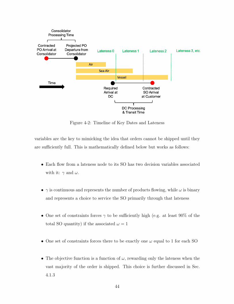
Figure 4-2: Timeline of Key Dates and Lateness

variables are the key to mimicking the idea that orders cannot be shipped until they

are sufficiently full. This is mathematically defined below but works as follows:

∙ Each flow from a lateness node to its SO has two decision variables associated

with it: 𝛾 and 𝜔.

∙ 𝛾 is continuous and represents the number of products flowing, while 𝜔 is binary

and represents a choice to service the SO primarily through that lateness

∙ One set of constraints forces 𝛾 to be sufficiently high (e.g. at least 90% of the

total SO quantity) if the associated 𝜔 = 1

∙ One set of constraints forces there to be exactly one 𝜔 equal to 1 for each SO

∙ The objective function is a function of 𝜔, rewarding only the lateness when the

vast majority of the order is shipped. This choice is further discussed in Sec.

4.1.3

44

4.1 Mathematical Model Definition

4.1.1 Decision Variables

The decision variables generally refer to the amount of product flowing on each of

the edges in Fig.4-1 shown as arrows labeled 𝛼, 𝛽, and 𝛾. The decision variables

labeled 𝜔 are binary variables described above. We also create a slack decision vari-

able 𝐿𝑎𝑛𝑒𝑆𝑙𝑎𝑐𝑘𝐶𝑛𝑡𝑟𝑦,𝑀𝑜𝑑𝑒 to help constrain the air freight capacity out of individual

countries depending on procured capacity.

∙ 𝛼𝑖,𝑗: This is a binary decision variable to denote that 𝑃𝑂𝑖 will travel by mode

j, where 𝑗 = 1, 2, 3 corresponding to vessel, sea air, and air modes, respectively.

Each 𝑃𝑂𝑖 will have three 𝛼𝑖,𝑗 variables associated with it representing the choice

of one of three modes. This decision variable is different from 𝛽 and 𝛾 in that it

does not represent the number of units flowing along the path. For constraint

sum notation, we define a set 𝐽𝑖 where |𝐽𝑖| = 3 and the elements are the three

indices of 𝑗 for the associated Air, Sea Air, and Vessel nodes.

∙ 𝛾𝑘,𝑙: These decision variables are similar to 𝛼𝑖,𝑗 and represent the lateness choices

for each SO (rather than the mode choices for each PO). For each SO 𝑙, the

first lateness defined is the earliest time that the first unit allocated to 𝑆𝑂𝑙 can

arrive by the fastest shipment mode. The last lateness is the latest time that

the last unit allocated to 𝑆𝑂𝑙 could arrive by the slowest shipment mode. All

lateness levels between these two boundary levels are also defined. Each 𝛾𝑘,𝑙 is

non-negative and represents the number of units on 𝑆𝑂𝑙 that are fulfilled via

lateness 𝑘. These values are most readily constrained by ship-ability constraints,

discussed more in Sec.4.1.3. Again for notation, we define a set 𝐾𝑙 where the

elements are the indices of 𝑘 associated with the various lateness times that can

service 𝑆𝑂𝑙.

∙ 𝛽𝑖,𝑗,𝑘,𝑙 : This is the number of units from PO 𝑖 shipped by mode 𝑗 to serve PO 𝑙

via lateness 𝑘. These variables are the flow from the mode nodes to the lateness

nodes and are the mechanism that link POs and SOs. This variable is created if

45

PO 𝑖 has product allocated to SO 𝑙 and choosing mode 𝑗 will allow that product

to arrive by lateness 𝑘. Like 𝛾, they are non-negative and represent number of

units flowing.

∙ 𝜔𝑘,𝑙: These binary decision variables are associated one-to-one with 𝛾𝑘,𝑙 and

represent the choice to service 𝑆𝑂𝑙 primarily through lateness 𝑘. As such,

exactly one 𝜔𝑘,𝑙 variable is required to equal one for each set of 𝑘 ∈ 𝐾𝑙.

4.1.2 Objective Function

As explained in Chap. 3, we have defined the relative value to the manufacturer

of various product categories as a function of lateness of the product and maximize

this value subject to budget constraints. This allows for a fairly simple objective

function. Each SO 𝑙 will have various quantities of different products, and the value

of all of these products being shipped at a certain lateness 𝑘 can be calculated and is

a constant for each SO and each lateness called 𝑉𝑘,𝑙. The objective function is then

simply the sum of these constants times the associated decision variable 𝜔𝑘,𝑙, a binary

decision signifying if that product was shipped at that lateness.

This has some drawbacks that will be discussed in Sec. 4.1.3 further, but allows

for a linear function of the value of the product dependent on when that product is

expected to leave the manufacturer’s distribution center for the customer. The model

is run with a budget constraint, then a pareto frontier is defined by running several

cases with various budget levels.

4.1.3 Constraints

The constraints can be broken into four general classes:

1. Balance Constraints: Force the flows into and out of each node to be equal.

2. Allocation Constraints: Force the product from a certain PO to flow to a

certain SO in some way to ensure all product goes where it was ordered.

46

3. Fill Rate Constraints: Forces one of the lateness nodes to have at least a

certain fraction of the total units for each SO. Meant to model requirements

at manufacturer’s distribution centers that require some amount of the product

for a certain order to be available before a job is created to pick, pack, and ship

that product.

4. Other Business Realities: Including system budget constraints, shipping

mode lane capacity constraints, and inability to split POs across multiple modes.

Using the sets of decision variables described above, the optimization problem

takes the following form.

47

max𝛼, 𝛽, 𝛾, 𝜔, 𝐿𝑎𝑛𝑒𝑆𝑙𝑎𝑐𝑘

∑︁𝑘,𝑙

𝑉𝑘,𝑙𝜔𝑘,𝑙 (4.1a)

s.t.∑︁𝑗

𝛼𝑖,𝑗 = 1 ∀ 𝑖, (4.1b)

𝛼𝑖,𝑗 * 𝑃𝑂𝐴𝑚𝑡𝑖 =∑︁𝑘,𝑙

𝛽𝑖,𝑗,𝑘,𝑙 ∀𝑗 ∈ 𝐽𝑖, ∀ 𝑖, (4.1c)

∑︁𝑗∈𝐽𝑖,𝑘∈𝐾𝑙

𝛽𝑖,𝑗,𝑘,𝑙 = 𝐴𝑙𝑙𝑜𝑐𝑄𝑡𝑦𝑖,𝑙 ∀{𝑖, 𝑙}, (4.1d)

∑︁𝑖,𝑗

𝛽𝑖,𝑗,𝑘,𝑙 = 𝛾𝑘,𝑙 ∀𝑘 ∈ 𝐾𝑙 ∀𝑙, (4.1e)

∑︁𝑘∈𝐾𝑙

𝜔𝑘,𝑙 = 1 ∀𝑙, (4.1f)

𝛾𝑘,𝑙 +𝑀 * (1− 𝜔𝑘,𝑙) ≥ 𝑆ℎ𝑖𝑝𝑇ℎ𝑟𝑒𝑠ℎ * 𝑆𝑂𝐴𝑚𝑡𝑙 ∀𝑘 ∈ 𝐾𝑙 ∀ 𝑙, (4.1g)∑︁𝑖,𝑗

𝐶𝑜𝑠𝑡𝑖,𝑗 * 𝛼𝑖,𝑗 +∑︁

𝐶𝑛𝑡𝑟𝑦,𝑀𝑜𝑑𝑒

𝐿𝑎𝑛𝑒𝑆𝑙𝑎𝑐𝑘𝐶𝑛𝑡𝑟𝑦,𝑀𝑜𝑑𝑒 *𝑂𝑣𝑒𝑟𝑎𝑔𝑒𝐶𝑛𝑡𝑟𝑦,𝑀𝑜𝑑𝑒≤ 𝑇𝑜𝑡𝑎𝑙𝐵𝑢𝑑𝑔𝑒𝑡,

(4.1h)∑︁𝑖∈𝐶𝑛𝑡𝑟𝑦,𝑗∈𝑀𝑜𝑑𝑒

𝑃𝑂𝐴𝑚𝑡𝑖 * 𝛼𝑖,𝑗 − 𝐿𝑎𝑛𝑒𝑆𝑙𝑎𝑐𝑘𝐶𝑛𝑡𝑟𝑦,𝑀𝑜𝑑𝑒 ≤ 𝐿𝑎𝑛𝑒𝑆𝑖𝑧𝑒𝐶𝑛𝑡𝑟𝑦,𝑀𝑜𝑑𝑒 ∀𝐶𝑛𝑡𝑟𝑦,𝑀𝑜𝑑𝑒,

(4.1i)

𝛼𝑖,𝑗 ∈ 0, 1, (4.1j)

𝛽𝑗,𝑘 ≥ 0, (4.1k)

𝛾𝑘,𝑙 ≥ 0, (4.1l)

𝜔𝑘,𝑙 ∈ 0, 1, (4.1m)

𝐿𝑎𝑛𝑒𝑆𝑙𝑎𝑐𝑘𝐶𝑛𝑡𝑟𝑦,𝑀𝑜𝑑𝑒 ≥ 0 (4.1n)

The four classes of constraints are discussed further below, non-negativity and

binary constraints 4.1j through 4.1n are discussed above in Sec. 4.1.1.

1. Balance Constraints: Constraints described by equations 4.1b, 4.1c, and

48

4.1e, ensure that product flows from PO nodes to SO nodes in one path. They

(in order) require one order to flow out of the ’PO’ node via exactly one of the

mode nodes, the binary mode choice to match with the equivalent units that

flow from the mode node to the lateness nodes, and finally from the lateness

nodes to the sales order nodes.

2. Allocation Constraints: Constraint 4.1d enforces the allocation of product

from purchase order 𝑖 to sales order 𝑙 by requiring the sum of all relevant 𝑏𝑒𝑡𝑎

variables to equal the allocation quantity constant (𝐴𝑙𝑙𝑜𝑐𝑄𝑡𝑦𝑖,𝑙).

3. Fill Rate Constraints: The order fill rate is governed by constraints 4.1f and

4.1g. Constraint 4.1g is a big M integer constraint requiring 𝛾 to exceed some

fraction of the total Sales Order (or shipment) quantity if the associated 𝜔 is

equal to one. Constraint 4.1f forces exactly one 𝜔 to equal one for each Sales

Order. The ShipThresh constant could in theory vary for each Sales Order,

but for most analyses presented in this thesis is set at 95% for all SOs. These

constraints represent another aspect of the service level that the manufacturer

delivers to its customers. When a shipment leaves the manufacturer’s distri-

bution center for delivery to the customer, a certain fraction (hopefully all) of

the order must be present in order for the order to meet contractual obligations

between the manufacturer and the retailer. In reality, these specifications can

be complex and specific, but this model approximates these requirements with

a simple requirement that at least some fraction (95%) of all product must be

present for the order to ship.

4. Other Business Realities: Constraint 4.1h restricts the total budget, while

4.1i restricts the shipment capacity by country while allowing for more expensive

per-unit overages via slack variables.

The way the objective function is formulated in combination with the fill rate

constraints is one high impact decision on the interpretability of the optimization.

There are two principal options: a weighting coefficient times each 𝜔 variable (used)

49

or a weighting coefficient times each 𝛽 variable (not used). Using 𝛽 or 𝜔 as the

decision variables in the objective are the two choices that maintain the spirit of the

Fill Rate constraint. Each has a benefit but also allows for different pathological cases

rewarding when product is actually delivered or rewarding when the order the product

is on satisfies the fill rate constraint. In each example, imagine a SO with several

different products, and relatively small amount (not enough to preclude satisfying

the shipment threshold constraint) of very valuable product.

When using 𝛽, we gain the benefit of only adding to the objective function when

each individual item arrives, but we could imagine a scenario where the valuable

product arrives very early, crediting the objective function for early delivery without

having enough of the order to allow for shipment that early. Conversely, while using

𝜔, the vast majority of product could arrive very early while the valuable product is

late. The order looks like it is ship-able early and the objective function is credited

for delivering the entire order, despite some valuable product arriving later.

The pathological 𝛽 case was deemed more likely to happen due to the low cost and

high reward of the case and the likelihood of additional business processes preventing

the pathological 𝜔 case with check-ins on valuable product. Therefore, we chose to

use 𝜔 as the decision variable in the objective function.

4.2 Sensitivities and Extensions

4.2.1 Parameter Sensitivity Analysis

The Mixed-Integer formulation of the model precluded the use of shadow prices on

constraints to easily determine the marginal impact of changes in constraints on the

objective function, so I evaluated the impact of changing the fill rate requirement for

shipments and the requirement that inbound orders be shipped as whole orders. The

first involves changing the 95% threshold discussed above to values of 50%, 80% and

90%, while the second involves relaxing the constraint that 𝛼 is a binary variable and

instead allowing it to take any value between 0 and 1.

50

For the fill rate constraint, the discussion immediately prior to this section is

highly relevant. When relaxing the constraint away from a 100% requirement, the

approximation of the entirety of the order being fulfilled in the week in which the

fill rate requirement is met becomes less accurate and the modeling suggestions more

tenuous to claim will lead to positive real world outcomes.

The 𝛼 decision variables can be relaxed from integer to continuous on the set

[0,1]. This means that only a fraction of the PO is shipped by certain modes instead

of the entire quantity of items being shipped together. The correlation to realizable

outcomes under the current setup becomes near impossible to draw, but the mod-

eled benefits do provide concrete business case grounding in the potential benefits

to implementing more advanced processes to allow for split shipments and partial

expediting. This would allow a PO that has mostly on-time product on it to carve

off part for air freight but leave the rest for vessel shipping.

4.2.2 Forecasted Demand

A third ‘parameter’ that I tested the sensitivity was more structural to the model–the

timing of the order and the requirement that the order be delivered when the customer

said it ought to arrive. Often times the actual consumer demand lags the customer

demand significantly. If the manufacturer can predict this lag and work to service

consumer demand, that would buy the supply chain time to use slower shipment

methods. The goal behind altering this constraint is to evaluate the benefit to inbound

shipment expediting if the manufacturer were better able to predict end consumers

consumption and deliver to customers to meet that demand in lieu of delivering to

the customers’ stated preferences. Many products are ordered on contracts that run

throughout the duration of the season, so customers may order several months of

supply on a contract for arrival at the beginning of the season, only to need a fraction

of the product immediately. While this is a small impact of a more parsimoniously

run supply chain, there should by myriad reasons for a just-in-time arrival system to

meet customer demand, and I investigated the impact on inbound freight expediting.

This is a two step process: first, finding consumer demand and the discrepancy

51

from customer’s stated demand, and second predicting this demand early enough to

differentiate the inbound freight service based on meeting consumer demand. In this

study, we use one customer as an example where the retailer has significant insight

into their operations and these data are readily available. This would require signif-

icant insight into point-of-sale data to understand how each customer sells products

to consumers, so I evaluated it on one customer first to identify the maximum op-

portunity size that could be attained before investing in premier consumer prediction

and stronger data sharing relationships.

52

Chapter 5

Optimization Results

The results presentation uses differences between scenarios to drive conclusions and

recommendations. The model is run with different constraint parameters and the

optimal output describes the set of actions that would elicit the best service level in

that situation. Specifically, the following three sets of scenarios form the basis of the

results:

1. Vessel Only: This case is a floor on the service level showing the best possible

service level if all products are forced to move through the slowest mode. This

case solves very quickly, as the mode choice decision variables are fixed for each

order, and the service levels are strictly increasing as earlier service levels are

chosen for each delivery.

2. As Planned and As Executed Reality: These cases are meant to mimic re-

ality and represent the service levels given the as planned transportation modes

(when the POs were originally written), and the as executed transportation

modes (after the one-month prior process to incrementally air freight prod-

ucts). The discrepancy between the two is the process that this tool aims to

augment: the manual switching of orders from slow to fast modes approximately

one month prior to shipment. Similar to the Vessel Only case, these cases take

the decisions about mode for each order as fixed and the model optimizes service

level quite simply.

53

3. Optimal Scenarios: These cases have unconstrained modes for each purchase

order and a budget constraint to restrict spend. Shipping orders by faster modes

incurs higher costs and penalizes the budget constraint. The model then can

fully optimize for shipment mode across the entire order book. Different cases

at different budget levels then create a pareto frontier delineating the trade offs

between cost and optimal service level.

5.1 Analysis of Potential Improvement

Below the results are discussed from one representative month: the data included are

the order book for one month of orders filtered to the product allocated to Distribution

Center orders for the top 20 customers who have received product by air freight (those

customers account for some 70% of air freight volume, while the Distribution Center

orders are about 50% of total volume, as discussed earlier). The resulting set of orders

is some 15,000 SOs and 20,000 POs, with over 600,000 possible combinations of PO,

shipment mode, lateness, and SO. These figures are relatively consistent across the

recent months used for internal analyses, and the results shown in the discussion

below are generally representative of the results in all months. This monthly analysis

filtered to customers with high air freight usage is the setup under which the model

will be run when implemented. These decisions are the ones the end users are looking

for guidance on as they represent the vast majority of the discretionary expedite

decisions.

The optimal scenarios sketch out a pareto frontier where service level is maximized

subject to budget constraints. The best strategy for the manufacturer under the

service level tradeoffs established by the perishability in Sec. 3.3 is at or between

one of the points labeled in orange in Fig. 5-1. The ‘As Planned’ scenario is made

months in advance when the orders are first written, so it is expected that the scenario

will not be optimal as more information becomes available. However, under the

current paradigm, the blue ‘As Executed’ scenario shows the current state after re-

evaluating the shipments prior to arrival at port. One way to examine the success of

54

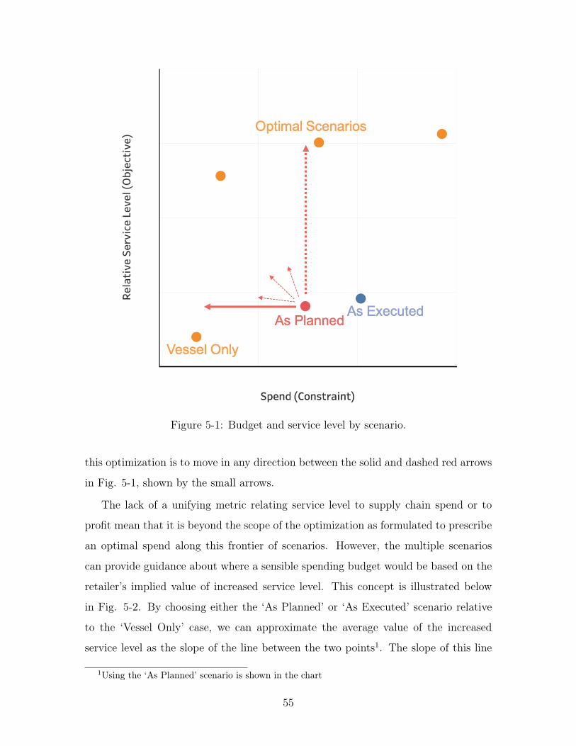
Figure 5-1: Budget and service level by scenario.

this optimization is to move in any direction between the solid and dashed red arrows

in Fig. 5-1, shown by the small arrows.

The lack of a unifying metric relating service level to supply chain spend or to

profit mean that it is beyond the scope of the optimization as formulated to prescribe

an optimal spend along this frontier of scenarios. However, the multiple scenarios

can provide guidance about where a sensible spending budget would be based on the

retailer’s implied value of increased service level. This concept is illustrated below

in Fig. 5-2. By choosing either the ‘As Planned’ or ‘As Executed’ scenario relative

to the ‘Vessel Only’ case, we can approximate the average value of the increased

service level as the slope of the line between the two points1. The slope of this line

1Using the ‘As Planned’ scenario is shown in the chart

55

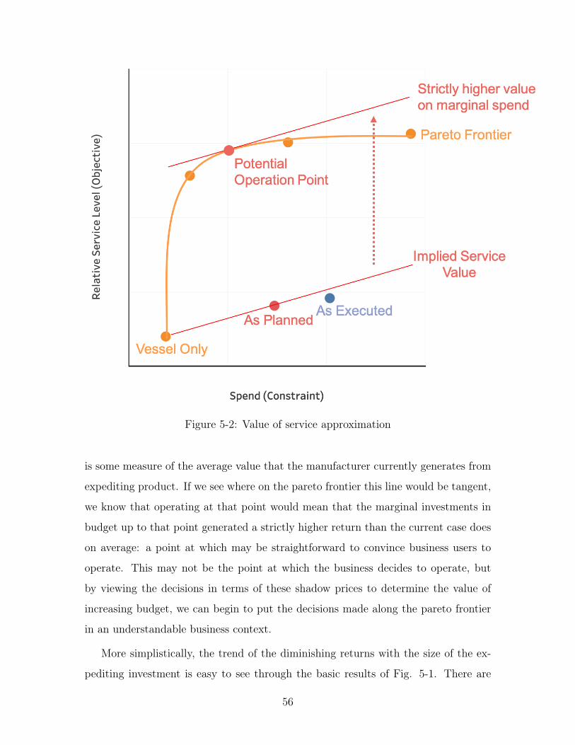
Figure 5-2: Value of service approximation

is some measure of the average value that the manufacturer currently generates from

expediting product. If we see where on the pareto frontier this line would be tangent,

we know that operating at that point would mean that the marginal investments in

budget up to that point generated a strictly higher return than the current case does

on average: a point at which may be straightforward to convince business users to

operate. This may not be the point at which the business decides to operate, but

by viewing the decisions in terms of these shadow prices to determine the value of

increasing budget, we can begin to put the decisions made along the pareto frontier

in an understandable business context.

More simplistically, the trend of the diminishing returns with the size of the ex-

pediting investment is easy to see through the basic results of Fig. 5-1. There are

56

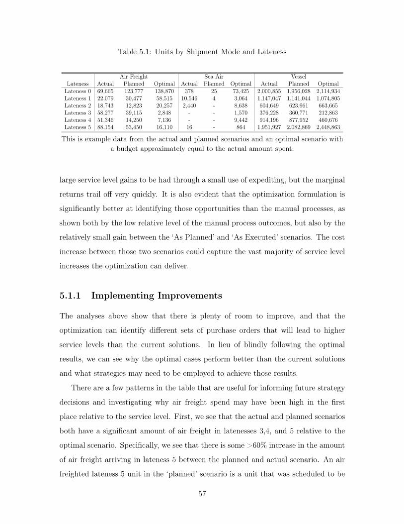
Table 5.1: Units by Shipment Mode and Lateness

Air Freight Sea Air VesselLateness Actual Planned Optimal Actual Planned Optimal Actual Planned Optimal

Lateness 0 69,665 123,777 138,870 378 25 73,425 2,000,855 1,956,028 2,114,934Lateness 1 22,079 30,477 58,515 10,546 4 3,064 1,147,047 1,141,044 1,074,805Lateness 2 18,743 12,823 20,257 2,440 - 8,638 604,649 623,961 663,665Lateness 3 58,277 39,115 2,848 - - 1,570 376,228 360,771 212,863Lateness 4 51,346 14,250 7,136 - - 9,442 914,196 877,952 460,676Lateness 5 88,154 53,450 16,110 16 - 864 1,951,927 2,082,869 2,448,863

This is example data from the actual and planned scenarios and an optimal scenario witha budget approximately equal to the actual amount spent.

large service level gains to be had through a small use of expediting, but the marginal

returns trail off very quickly. It is also evident that the optimization formulation is

significantly better at identifying those opportunities than the manual processes, as

shown both by the low relative level of the manual process outcomes, but also by the

relatively small gain between the ‘As Planned’ and ‘As Executed’ scenarios. The cost

increase between those two scenarios could capture the vast majority of service level

increases the optimization can deliver.

5.1.1 Implementing Improvements

The analyses above show that there is plenty of room to improve, and that the

optimization can identify different sets of purchase orders that will lead to higher

service levels than the current solutions. In lieu of blindly following the optimal

results, we can see why the optimal cases perform better than the current solutions

and what strategies may need to be employed to achieve those results.

There are a few patterns in the table that are useful for informing future strategy

decisions and investigating why air freight spend may have been high in the first

place relative to the service level. First, we see that the actual and planned scenarios

both have a significant amount of air freight in latenesses 3,4, and 5 relative to the

optimal scenario. Specifically, we see that there is some >60% increase in the amount

of air freight arriving in lateness 5 between the planned and actual scenario. An air

freighted lateness 5 unit in the ‘planned’ scenario is a unit that was scheduled to be

57

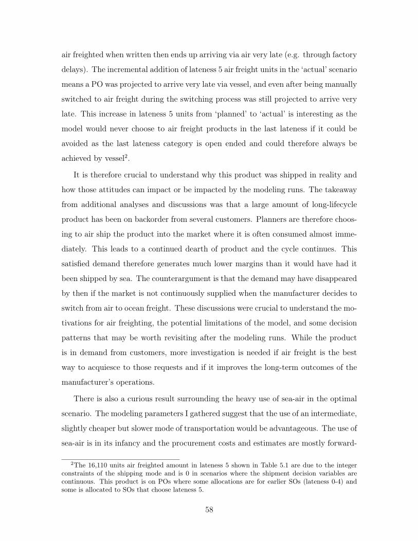
air freighted when written then ends up arriving via air very late (e.g. through factory

delays). The incremental addition of lateness 5 air freight units in the ‘actual’ scenario

means a PO was projected to arrive very late via vessel, and even after being manually

switched to air freight during the switching process was still projected to arrive very

late. This increase in lateness 5 units from ‘planned’ to ‘actual’ is interesting as the

model would never choose to air freight products in the last lateness if it could be

avoided as the last lateness category is open ended and could therefore always be

achieved by vessel2.

It is therefore crucial to understand why this product was shipped in reality and

how those attitudes can impact or be impacted by the modeling runs. The takeaway

from additional analyses and discussions was that a large amount of long-lifecycle

product has been on backorder from several customers. Planners are therefore choos-

ing to air ship the product into the market where it is often consumed almost imme-

diately. This leads to a continued dearth of product and the cycle continues. This

satisfied demand therefore generates much lower margins than it would have had it

been shipped by sea. The counterargument is that the demand may have disappeared

by then if the market is not continuously supplied when the manufacturer decides to

switch from air to ocean freight. These discussions were crucial to understand the mo-

tivations for air freighting, the potential limitations of the model, and some decision

patterns that may be worth revisiting after the modeling runs. While the product

is in demand from customers, more investigation is needed if air freight is the best

way to acquiesce to those requests and if it improves the long-term outcomes of the

manufacturer’s operations.

There is also a curious result surrounding the heavy use of sea-air in the optimal

scenario. The modeling parameters I gathered suggest that the use of an intermediate,

slightly cheaper but slower mode of transportation would be advantageous. The use of

sea-air is in its infancy and the procurement costs and estimates are mostly forward-

2The 16,110 units air freighted amount in lateness 5 shown in Table 5.1 are due to the integerconstraints of the shipping mode and is 0 in scenarios where the shipment decision variables arecontinuous. This product is on POs where some allocations are for earlier SOs (lateness 0-4) andsome is allocated to SOs that choose lateness 5.

58

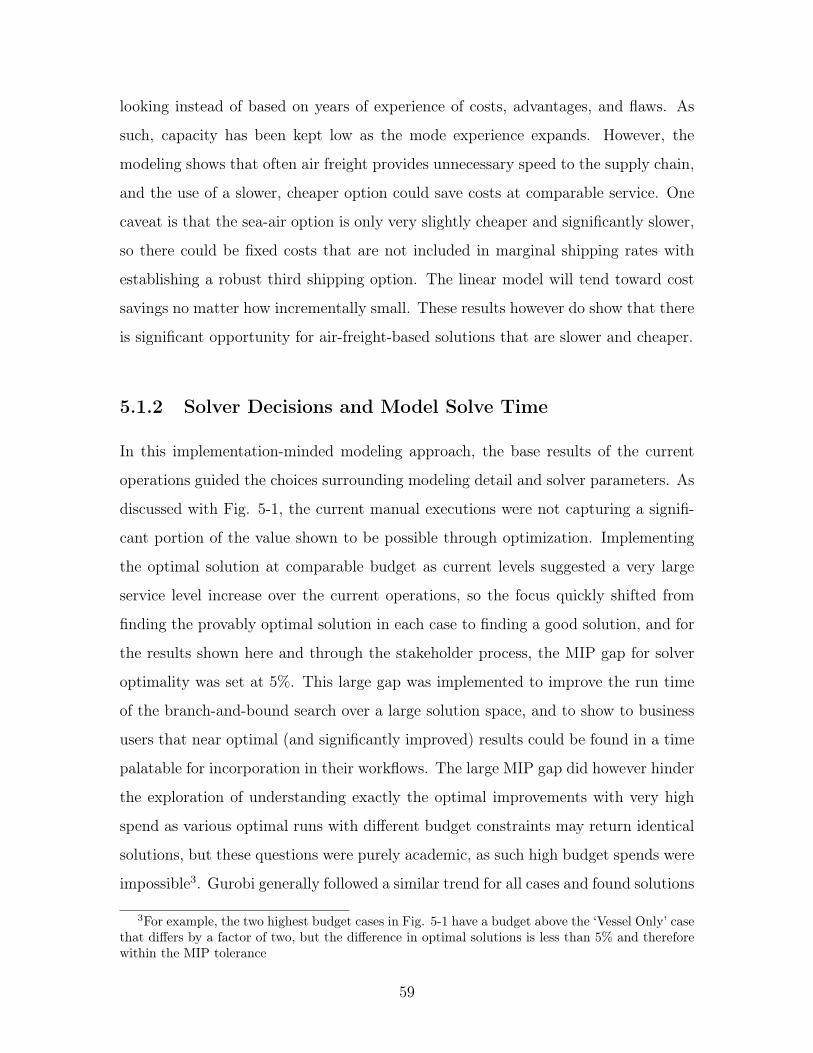
looking instead of based on years of experience of costs, advantages, and flaws. As

such, capacity has been kept low as the mode experience expands. However, the

modeling shows that often air freight provides unnecessary speed to the supply chain,

and the use of a slower, cheaper option could save costs at comparable service. One

caveat is that the sea-air option is only very slightly cheaper and significantly slower,

so there could be fixed costs that are not included in marginal shipping rates with

establishing a robust third shipping option. The linear model will tend toward cost

savings no matter how incrementally small. These results however do show that there

is significant opportunity for air-freight-based solutions that are slower and cheaper.

5.1.2 Solver Decisions and Model Solve Time

In this implementation-minded modeling approach, the base results of the current

operations guided the choices surrounding modeling detail and solver parameters. As

discussed with Fig. 5-1, the current manual executions were not capturing a signifi-

cant portion of the value shown to be possible through optimization. Implementing

the optimal solution at comparable budget as current levels suggested a very large

service level increase over the current operations, so the focus quickly shifted from

finding the provably optimal solution in each case to finding a good solution, and for

the results shown here and through the stakeholder process, the MIP gap for solver

optimality was set at 5%. This large gap was implemented to improve the run time

of the branch-and-bound search over a large solution space, and to show to business

users that near optimal (and significantly improved) results could be found in a time

palatable for incorporation in their workflows. The large MIP gap did however hinder

the exploration of understanding exactly the optimal improvements with very high

spend as various optimal runs with different budget constraints may return identical

solutions, but these questions were purely academic, as such high budget spends were

impossible3. Gurobi generally followed a similar trend for all cases and found solutions

3For example, the two highest budget cases in Fig. 5-1 have a budget above the ‘Vessel Only’ casethat differs by a factor of two, but the difference in optimal solutions is less than 5% and thereforewithin the MIP tolerance

59

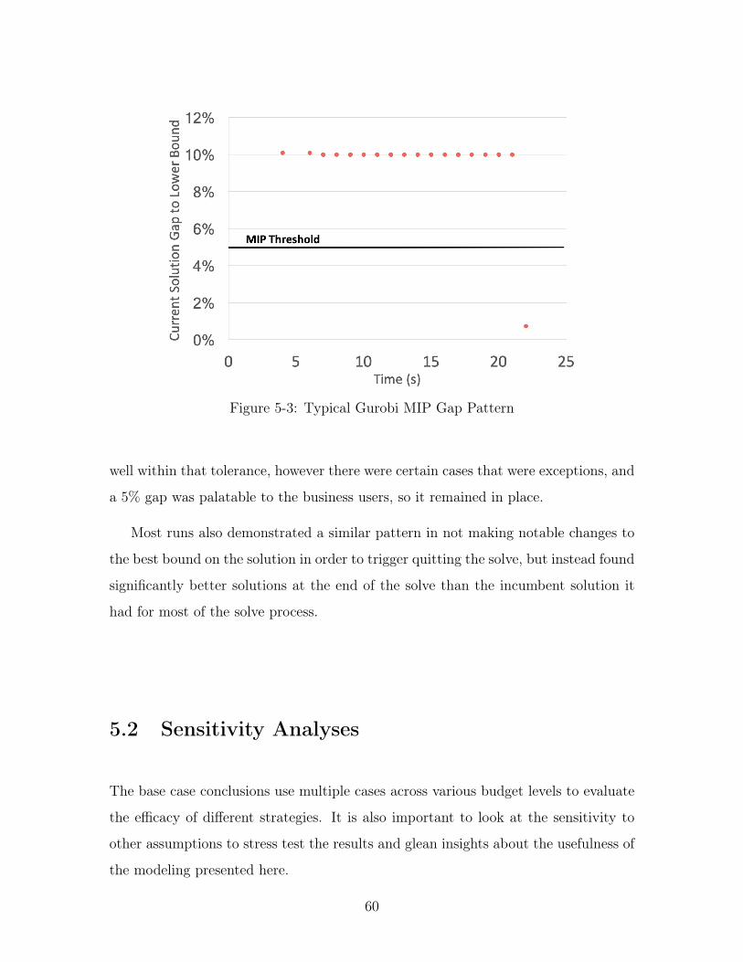
Figure 5-3: Typical Gurobi MIP Gap Pattern

well within that tolerance, however there were certain cases that were exceptions, and

a 5% gap was palatable to the business users, so it remained in place.

Most runs also demonstrated a similar pattern in not making notable changes to

the best bound on the solution in order to trigger quitting the solve, but instead found

significantly better solutions at the end of the solve than the incumbent solution it

had for most of the solve process.

5.2 Sensitivity Analyses

The base case conclusions use multiple cases across various budget levels to evaluate

the efficacy of different strategies. It is also important to look at the sensitivity to

other assumptions to stress test the results and glean insights about the usefulness of

the modeling presented here.

60

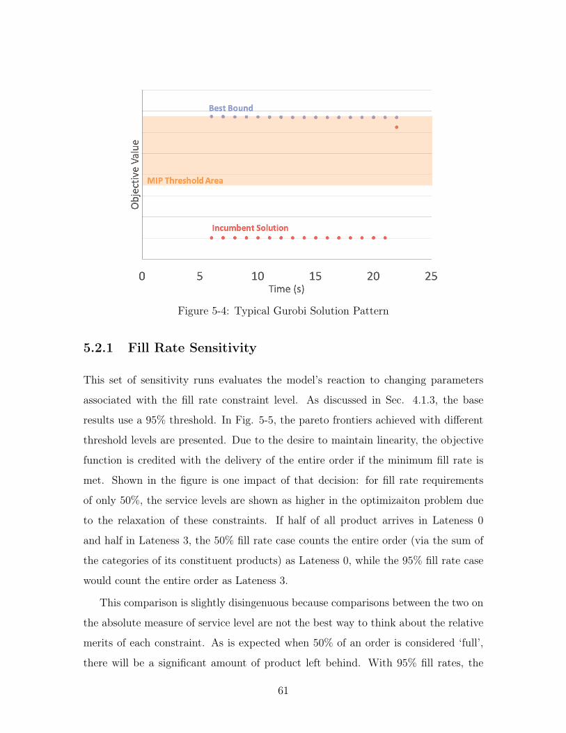
Figure 5-4: Typical Gurobi Solution Pattern

5.2.1 Fill Rate Sensitivity

This set of sensitivity runs evaluates the model’s reaction to changing parameters

associated with the fill rate constraint level. As discussed in Sec. 4.1.3, the base

results use a 95% threshold. In Fig. 5-5, the pareto frontiers achieved with different

threshold levels are presented. Due to the desire to maintain linearity, the objective

function is credited with the delivery of the entire order if the minimum fill rate is

met. Shown in the figure is one impact of that decision: for fill rate requirements

of only 50%, the service levels are shown as higher in the optimizaiton problem due

to the relaxation of these constraints. If half of all product arrives in Lateness 0

and half in Lateness 3, the 50% fill rate case counts the entire order (via the sum of

the categories of its constituent products) as Lateness 0, while the 95% fill rate case

would count the entire order as Lateness 3.

This comparison is slightly disingenuous because comparisons between the two on

the absolute measure of service level are not the best way to think about the relative

merits of each constraint. As is expected when 50% of an order is considered ‘full’,

there will be a significant amount of product left behind. With 95% fill rates, the

61

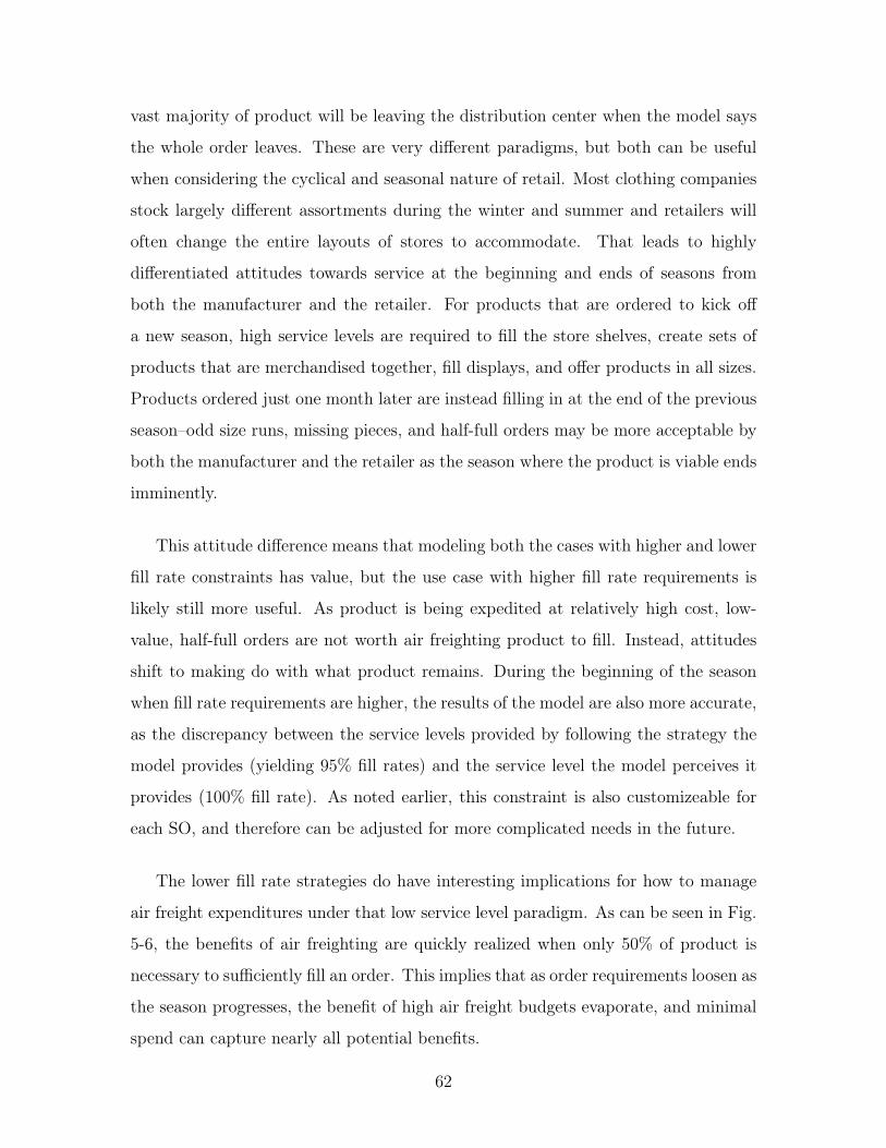
vast majority of product will be leaving the distribution center when the model says

the whole order leaves. These are very different paradigms, but both can be useful

when considering the cyclical and seasonal nature of retail. Most clothing companies

stock largely different assortments during the winter and summer and retailers will

often change the entire layouts of stores to accommodate. That leads to highly

differentiated attitudes towards service at the beginning and ends of seasons from

both the manufacturer and the retailer. For products that are ordered to kick off

a new season, high service levels are required to fill the store shelves, create sets of

products that are merchandised together, fill displays, and offer products in all sizes.

Products ordered just one month later are instead filling in at the end of the previous

season–odd size runs, missing pieces, and half-full orders may be more acceptable by

both the manufacturer and the retailer as the season where the product is viable ends

imminently.

This attitude difference means that modeling both the cases with higher and lower

fill rate constraints has value, but the use case with higher fill rate requirements is

likely still more useful. As product is being expedited at relatively high cost, low-

value, half-full orders are not worth air freighting product to fill. Instead, attitudes

shift to making do with what product remains. During the beginning of the season

when fill rate requirements are higher, the results of the model are also more accurate,

as the discrepancy between the service levels provided by following the strategy the

model provides (yielding 95% fill rates) and the service level the model perceives it

provides (100% fill rate). As noted earlier, this constraint is also customizeable for

each SO, and therefore can be adjusted for more complicated needs in the future.

The lower fill rate strategies do have interesting implications for how to manage

air freight expenditures under that low service level paradigm. As can be seen in Fig.

5-6, the benefits of air freighting are quickly realized when only 50% of product is

necessary to sufficiently fill an order. This implies that as order requirements loosen as

the season progresses, the benefit of high air freight budgets evaporate, and minimal

spend can capture nearly all potential benefits.

62

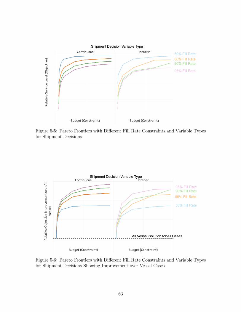
Figure 5-5: Pareto Frontiers with Different Fill Rate Constraints and Variable Typesfor Shipment Decisions

Figure 5-6: Pareto Frontiers with Different Fill Rate Constraints and Variable Typesfor Shipment Decisions Showing Improvement over Vessel Cases

63

5.2.2 Discrete Mode Choice Relaxation

The simple implementation of this modeling would require that each purchase order

is shipped in its entirety via one mode. A dynamic supply chain may be able to split

up orders and ship only a portion of the order by each mode, expediting only what

is necessary and sending the rest by sea. To model this, we relax the constraint that

the 𝛼 decision variables for each order must be binary, and instead allow it to take

any value between 0 and 1. The constraint requiring the sum of all 𝛼 for each order

equal 1 remains. The comparisons between the cases requiring integer solutions and

allowing for continuous relaxations can be seen in Figs. 5-5 and 5-6.

Fig. 5-6 shows the trends present particularly well. The continuous relaxation

consistently outperforms the integer formulation at similar budget levels and reaches

the plateau earlier where additional spend does not increase service levels. For lower

fill rate constraints like the blue 50% constraint curves, the two curves do reach

similar points eventually. However, for the more heavily constrained models like the

purple 95% curves, the continuous relaxation continues to substantially outperform

its integer equivalent.

This relatively better performance is operationally irrelevant however. The oper-

ational complexity of changing logistics software, shipping and receiving processing,

and other infrastructure to accommodate split shipments is likely to not be worth

the incremental payoff. There are bound to be plenty of challenges with the current

implementation of this analysis, and the order of magnitude of possible service level

increases or cost reductions are quite similar to the split shipments case. For an

illustration of these scale differences, see Fig. 5-7.

5.2.3 Deliver-to-need

Customers often place a contract style order with the manufacturer. This contract

allows for a reservation of units at the manufacturer’s DC with smaller shipments

calling off the units on that contract over the course of the season. If the manufacturer

air freights the entire contracted amount into the DC at the beginning of the season,

64

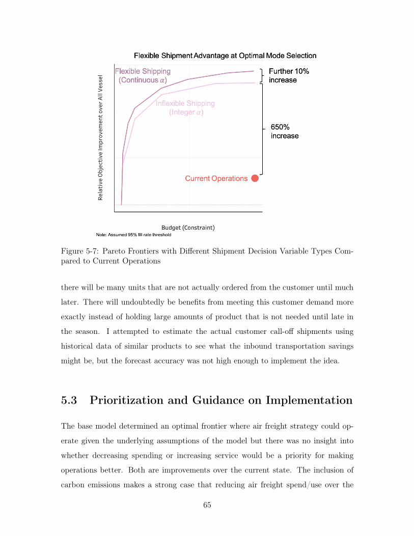
Figure 5-7: Pareto Frontiers with Different Shipment Decision Variable Types Com-pared to Current Operations

there will be many units that are not actually ordered from the customer until much

later. There will undoubtedly be benefits from meeting this customer demand more

exactly instead of holding large amounts of product that is not needed until late in

the season. I attempted to estimate the actual customer call-off shipments using

historical data of similar products to see what the inbound transportation savings

might be, but the forecast accuracy was not high enough to implement the idea.

5.3 Prioritization and Guidance on Implementation

The base model determined an optimal frontier where air freight strategy could op-

erate given the underlying assumptions of the model but there was no insight into

whether decreasing spending or increasing service would be a priority for making

operations better. Both are improvements over the current state. The inclusion of

carbon emissions makes a strong case that reducing air freight spend/use over the

65

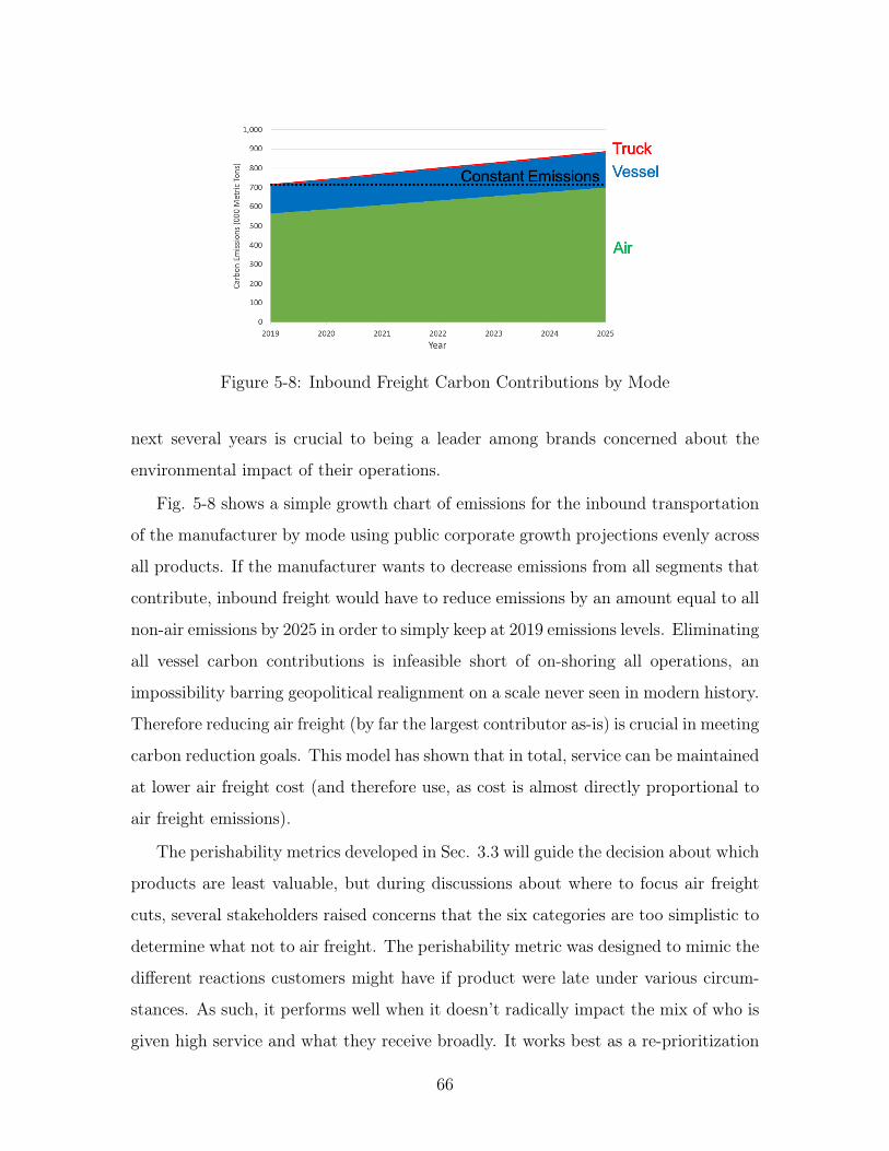
Figure 5-8: Inbound Freight Carbon Contributions by Mode

next several years is crucial to being a leader among brands concerned about the

environmental impact of their operations.

Fig. 5-8 shows a simple growth chart of emissions for the inbound transportation

of the manufacturer by mode using public corporate growth projections evenly across

all products. If the manufacturer wants to decrease emissions from all segments that

contribute, inbound freight would have to reduce emissions by an amount equal to all

non-air emissions by 2025 in order to simply keep at 2019 emissions levels. Eliminating

all vessel carbon contributions is infeasible short of on-shoring all operations, an

impossibility barring geopolitical realignment on a scale never seen in modern history.

Therefore reducing air freight (by far the largest contributor as-is) is crucial in meeting

carbon reduction goals. This model has shown that in total, service can be maintained

at lower air freight cost (and therefore use, as cost is almost directly proportional to

air freight emissions).

The perishability metrics developed in Sec. 3.3 will guide the decision about which

products are least valuable, but during discussions about where to focus air freight

cuts, several stakeholders raised concerns that the six categories are too simplistic to

determine what not to air freight. The perishability metric was designed to mimic the

different reactions customers might have if product were late under various circum-

stances. As such, it performs well when it doesn’t radically impact the mix of who is

given high service and what they receive broadly. It works best as a re-prioritization

66

of the existing order book. The reaction to a late key launch-day style is different to

late long-lifecycle product and perishability captures that well. However, with large

changes in service, a poor reaction from customer A may be received internally dif-

ferently from customer B. Late product in category Z with a large marketing budget

and high price point may be more important that category Y, with small marketing

outlays and low prices.

Combining these effects with a recommended carbon price4 reveals some interest-

ing trends in profitability of different product categories when carbon is taken into

account. This analysis estimates the average profit for a large class of products (e.g.

dollars earned per unit for all running shoes) that the manufacturer earns when selling

to customers. Then, a per-unit air freight cost is subtracted, including both the cost

charged by the shipper and the implied cost of emitted carbon. The dollar values are

suppressed, but we can see in Fig. 5-9 that several categories would not earn a profit

for the manufacturer. If the manufacturer implemented carbon pricing and continued

air freighting these classes of product, they would effectively be selling product at a

loss. For example, Category 3 would be a candidate for halting air freight as it is

high volume, but has no profitability once air freighted.

There are many ways forward incorporating this data including further scaling

or segmenting perishability values by profit margin, or capping quantities of less

profitable categories. Both would result in prioritizing the least profitable categories

to reduce air freight quantities.

4$100/MT is the assumption from the UN global compact(https://www.unglobalcompact.org/take-action/action/carbon)

67

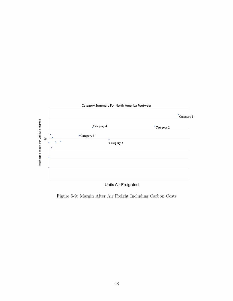
Figure 5-9: Margin After Air Freight Including Carbon Costs

68

Chapter 6

Conclusions and Future Work

In this thesis, I developed a network optimization approach to improve the outcomes

of expediting inbound freight orders for a brand with distributed manufacturing and

multiple customers. The approach determined the optimal transportation mode for

each order from contract manufacturers and the optimal lateness at which to fulfill

each shipment to customers. Among the many constraints on the system were the

budget available for transportation costs, the fill rate of shipments, and the allocation

of products from orders to shipments. The optimization used product categorization

and valuation from business users of the tool to inform the value of on-time products

and the rate at which various categories degraded in value with increasing lateness.

Tests of the model at a large retail brand showed that the vast majority of service

level gains come from the initial spend beyond the minimum required by the cheapest

transportation mode, and that marginal returns to increased spend decline quickly.

There are three major categories of future work that could help to improve this

models applicability, potentially partially mutually exclusive: simplification, formu-

lation developments, and parameter improvements.

Simplification: A simpler model will be easier to understand for end users and

faster to run. Run time increases could make more scenarios with different parameters

easy to test, make solving the model in real-time during meetings and conversations

feasible. The run time decreases due to loosening model solver restrictions did leave

to scenarios that took minutes to run, but for a solution to be truly scaleable to

69

the entire order book and for planners to have the ability to test new ideas in real

time, the solve time will need to decrease. A simpler model will also likely aid the

interpretability of the results and make for clearer decisions based off of the results

Formulation Developments: Another direction to move this work is one of

additional complexity, if not in modeling mathematics then in conceptual design and

applicability. One key assumption that could be broken in the modeling is the idea

that all units from a given PO are mapped to a specific SO. In reality, there is some

re-shuffling that can be done to pool all different orders of product A and optimally

allocate the on-hand and pipeline inventory of product A across all different ship-

ments that have requested product A. This approach may need to more explicitly

model the on-hand inventory within warehouses, and its applicability requires a more

flexible treatment of inventory in reality. The model explored in this thesis has the

advantage of a given unit being earmarked for a specific shipment, which may be

the best approach for satisfying customers and organizing the supply chain. Break-

ing this assumption could lead to a much more powerful model to not only expedite

what is necessary but to allocate exiting inventory optimally across different cus-

tomer requests. With this increased scope and power, however may come a decreased

application to the problem of optimizing air freight decisions.

Parameter Improvement: Perhaps the most realistic and obvious next step

is to better inform parameters through data analysis, rather than via human input.

This model relied quite heavily on a stakeholder-based method to discuss the various

categories of products and their relative values to use as weights in the objective

function. These constituent weights 𝑣𝑝,𝑙 as discussed in Sec. 4.1.2 are designed to

best mimic what the people running the decision process intend to happen. This has

a tremendous amount of value both in the decisions it generates, but also in helping to

solicit buy-in from the interested stakeholders that the model will not be dramatically

changing outcomes, but instead making more consistent decisions.

Informing these parameters using sell-through rates, forecasted demand, market-

ing spend, and better understanding of the value that marginal improvements in

service levels to customers bring to the manufacturer would be one way to imbibe

70

the entire decision making process with consumer-based data and to make better de-

cisions overall. In attempting to use a data-driven approach to inform these values,

I found that the supply chain data availability were inadequate to meet the needs of

other interested stakeholders, and that analysing this marginal value would require

much more data from across the enterprise that was not available or was controlled by

areas without a strong sponsor and understanding of the supply chain impact of their

data. In a future state with centralized, accessible data regarding the preferences of

disparate business units, this type of analysis may be feasible and fruitful.

71

72

Bibliography

[1] Adidas AG. 2019 factory list. https://www.adidas-group.com/en/sustainability/managing-sustainability/human-rights/supply-chain-structure/, 2019.

[2] Juan José Bravo and Carlos Julio Vidal. Freight transportation function insupply chain optimization models: A critical review of recent trends. ExpertSystems with Applications, 40(17):6742–6757, 2013.

[3] Y Cardona-Valdés, A Álvarez, and D Ozdemir. A bi-objective supply chaindesign problem with uncertainty. Transportation Research Part C: EmergingTechnologies, 19(5):821–832, 2011.

[4] Chevron. Climate change initiatives. https://www.chevron.com/corporate-responsibility/climate-change, Oct 2019.

[5] Tom Crabtree, Tom Hoang, Russel Tom, and Gregg Gildemann. World air cargoforecast 2018-2037, 2018.

[6] John H Cushman. Industrial group plans to battle climate treaty. The New YorkTimes, page 1, Apr 1998.

[7] Ali Diabat and David Simchi-Levi. A carbon-capped supply chain network prob-lem. In 2009 IEEE international conference on industrial engineering and engi-neering management, pages 523–527. IEEE, 2009.

[8] Ashton Imlay. Massachusetts Institute of Technology. Improving order prioriti-zation for the allocation of constrained supply, 2019.

[9] Nike Inc. Annual report, 1987.

[10] Nike Inc. Annual report, 1999.

[11] Nike Inc. Consumer direct offense. https://news.nike.com/news/nike-consumer-direct-offense, June 2017.

[12] Nike Inc. Form 10-k 2019. https://www.sec.gov/Archives/edgar/data/320187/000032018719000051/nke-531201910k.htm, May 2019.

[13] AT Kearney. Council of supply chain management professional’s annual state oflogistics report, 2017.

73

[14] Intergovernmental Panel on Climate Change. Ipcc special report on global warm-ing of 1.5 degrees celsius. https://www.ipcc.ch/sr15/, 2018.

[15] International Maritime Organization. Second imo ghg study.http://www.imo.org/en/OurWork/Environment/PollutionPrevention/AirPollution/Documents/SecondIMOGHGStudy2009.pdf, 2009.

[16] Turan Paksoy, Eren Özceylan, and Gerhard-Wilhelm Weber. Profit orientedsupply chain network optimization. Central European Journal of OperationsResearch, 21(2):455–478, 2013.

[17] Bruno Sarda. How corporate america is addressing climate change risks.https://www.wbur.org/hereandnow/2019/07/09/corporate-america-addresses-climate-change, Jul 2019.

[18] Jared Vineyard. Could cargo ships get a speed limit? Universal Cargo, page 1,May 2019.

[19] Andreas Wiesmann. Slow steaming: a viable long-term option?https://www.wartsila.com/docs/default-source/Service-catalogue-files/Engine-Services—2-stroke/slow-steaming-a-viable-long-term-option.pdf, 2010.

74