Embed Size (px)
Citation preview

Optimizing the Spinning
Reserve Requirements
A thesis submitted to the University of Manchester for the degree of
Doctor of Philosophy
in the Faculty of Engineering and Physical Sciences
May 2006
Miguel Angel Ortega Vazquez
School of Electrical and Electronic Engineering

Table of Contents ____________________________________________________________________
2
Table of Contents
TABLE OF CONTENTS 2
ABSTRACT 6
DECLARATION 7
COPYRIGHT STATEMENT 8
ABOUT THE AUTHOR 9
ACKNOLEGEMENTS 10
LIST OF PUBLICATIONS 11
LIST OF FIGURES 12
LIST OF TABLES 18
LIST OF SYMBOLS 20
LIST OF ACCRONYMS 23
1. INTRODUCTION 25
1.1. Background …………………………………………………………… 25
1.2. Fixed Spinning Reserve Requirements ………………………………… 26
1.3. Problem Identification ………………………………………………… 31
1.4. Bibliography Survey …………………………………………………… 34
1.5. Proposed Formulations ………………………………………………… 39
1.6. Outline of the Thesis …………………………………………………… 40
2. TRADITIONAL AND PROPOSED UNIT COMMITMENT 43
2.1. Introduction …………………………………………………………… 43
2.2. Unit Commitment Formulation ………………………………………… 44
2.2.1. Objective Function ……………………………………………… 44
2.2.2. Cost Function …………………………………………………… 44
2.2.3. Start-up Cost …………………………………………………… 45
2.2.4. Power Balance ………………………………………………… 46
2.2.5. Spinning Reserve Requirement ………………………………… 46
2.2.6. Power Output Limits …………………………………………… 46

Table of Contents ____________________________________________________________________
3
2.2.7. Minimum–up and –down Times ………………………………… 47
2.2.8. Ramp–up and –down Limits …………………………………… 47
2.3. Proposed Theoretical UC Approach …………………………………… 49
2.3.1. Proposed Objective Function …………………………………… 49
2.4. Expected Cost of Deprived Energy …………………………………… 50
2.5. Implementation of the Proposed Approach …………………………… 51
2.5.1. Spinning Reserve Requirements, Unit’s Scheduling and VOLL .. 54
2.5.2. Optimal Scheduling and Load Variations ……………………… 56
2.5.3. Optimal Scheduling and LOLP ………………………………… 58
2.5.4. Comparison of the Different Approaches ……………………… 61
2.6. Conclusions …………………………………………………………… 65
3. OPTIMAL SCHEDULING OF SPINNING RESERVE WITH AN EENS
PROXY 67
3.1. Introduction …………………………………………………………… 67
3.2. Proposed Unit Commitment Formulation ……………………………… 68
3.3. EENS Approximation ………………………………………………… 69
3.3.1. Relationship Between EENS and Committed Capacity ………… 69
3.4. EENS Piecewise Linear Approximation ……………………………… 72
3.5. Accuracy of the Approximation ……………………………………… 76
3.6. Implementation of the Proposed UC …………………………………… 78
3.7. Test Results …………………………………………………………… 83
3.7.1. Results on the IEEE-RTS Single-Area System ………………… 83
3.7.2. Results on the IEEE-RTS Three-Area System ………………… 89
3.8. Conclusions …………………………………………………………… 94
4. OPTIMAL SCHEDULING OF SPINNING RESERVE CONSIDERING
THE FAILURE TO SYNCHRONIZE WITH EENS PROXIES 96
4.1. Introduction …………………………………………………………… 96
4.2. Generating Unit Models ……………………………………………… 97
4.2.1. Unit Operating States …………………………………………… 97
4.2.2. Two-State Model ……………………………………………… 99
4.2.3. Four-State Model ……………………………………………… 100
4.3. EENS Calculation …………………………………………………… 105
4.4. Model Validation Using Monte Carlo Methods ……………………… 109
4.5. Time Decoupled Unit Commitment ………………………………… 112

Table of Contents ____________________________________________________________________
4
4.6. Maximum Capacity on Synchronization ……………………………… 114
4.7. EENS Behaviour as a Function of the CS …………………………… 115
4.8. EENS Approximation as a Function of the CS ……………………… 118
4.9. Implementation of the Proposed UC Approach ……………………… 124
4.10. Test Results ………………………………………………………… 131
4.10.1. Test Results in the IEEE-RTS Single-Area System …………… 131
4.10.2. Test Results in the IEEE-RTS Three-Area System …………… 135
4.11. Conclusions ………………………………………………………… 139
5. OPTIMIZING THE SPINNING RESERVE REQUIREMENTS 140
5.1. Introduction …………………………………………………………… 140
5.2. Proposed Approach Description ……………………………………… 142
5.2.1. Optimal SR Requirements …………………………………… 143
5.2.1.1.Running Cost ……………………………………………… 144
5.2.1.2.EENS Cost ………………………………………………… 145
5.2.2. Three-Point Grid Search ……………………………………… 146
5.2.3. Unit Commitment ……………………………………………… 150
5.3. Test Results …………………………………………………………… 151
5.3.1. Effect of the Generation Schedule …………………………… 151
5.3.2. Effect of the System Size and Load Level …………………… 153
5.3.3. Effect of the Unit’s ORR ……………………………………… 156
5.3.4. Effect of the VOLL …………………………………………… 157
5.3.5. Cost Itemization ……………………………………………… 159
5.3.6. Other Fixed SR Requirements and VOLL …………………… 161
5.3.7. Hybrid Approach ……………………………………………… 164
5.3.8. Computation Time …………………………………………… 166
5.4. Conclusions …………………………………………………………… 166
6. ECONOMIC IMPACT ASSESSMENT OF LOAD FORECAST ERRORS
CONSIDERING THE COST OF INTERRUPTIONS 168
6.1. Introduction …………………………………………………………… 168
6.2. Review of Previous Work …………………………………………… 169
6.3. Identification of the Costs …………………………………………… 170
6.4. Spinning Reserve, Re-dispatch and Load Forecast Errors …………… 171
6.5. Economic Impact Calculation ………………………………………… 174
6.5.1. Gather Information of the Power System ……………………… 174

Table of Contents ____________________________________________________________________
5
6.5.2. Compute the UC for the Actual Load ………………………… 174
6.5.3. Operating Cost Calculation …………………………………… 175
6.5.4. Simulate Load Forecasting …………………………………… 176
6.5.5. Run UC for the Forecasted Load ……………………………… 177
6.5.6. Re-Schedule to Meet the Actual Demand …………………… 177
6.5.7. Compute the Economic Impact ……………………………… 178
6.5.8. Meet the Monte Carlo Convergence Criterion ………………… 178
6.6. Test Results …………………………………………………………… 179
6.6.1. Effect of the Load Forecast Accuracy ………………………… 179
6.6.2. Effect of the Correlation Window Width ……………………… 181
6.6.3. Effect of the VOLL …………………………………………… 184
6.7. Conclusions …………………………………………………………… 186
7. CONCLUSIONS AND SUGGESTIONS FOR FURTHER WORK 187
7.1. Conclusions …………………………………………………………… 187
7.2. Suggestions for Further Work ………………………………………… 190
A. FAILURE PROBABILITIES 193
A.1 Generating Units’ Outage Probabilities ……………………………… 193
B. SYSTEMS DATA 195
B.1 26-Unit System ……………………………………………………… 195
B.2 76-Unit System ……………………………………………………… 198
C. MIXED INTEGER LINEAR PROGRAMMING MODELS 202
C.1 Cost Function ………………………………………………………… 202
C.2 Generation Limits …………………………………………………… 203
C.3 Start-up Cost ………………………………………………………… 204
C.4 Power Balance ……………………………………………………… 205
C.5 Spinning Reserve Requirement ……………………………………… 205
C.6 Minimum-up and –down Times……………………………………… 207
C.7 Ramp-up and –down Limits ………………………………………… 207
C.8 Piecewise Cost Function Data: 26-Unit System …………………… 210
C.9 Piecewise Cost Function Data: 78-Unit System …………………… 211
REFERENCES 214

6
Abstract
Spinning reserve is probably the most important resource used by power system
operators to respond to sudden generation outages and prevent load disconnections.
While its availability has a substantial value because it mitigates the considerable
social and economic cost of outages, the provision of spinning reserve is costly.
Over-scheduling spinning reserve results in high operating costs while under-
scheduling it results in a larger security risk for the power system, which can lead to
load shedding in case of contingencies.
Unit commitment programs customarily include a reserve constraint in their
optimization procedure to ensure that a fixed amount of spinning reserve is
scheduled. This fixed spinning reserve requirement is obtained from standards
developed off-line for each power system. Providing this amount of spinning reserve
at all periods of the optimization horizon is sub-optimal because it considers
explicitly neither the cost of its provision, nor the value that consumers place on not
being disconnected. In practice this means that the amount of spinning reserve
scheduled is likely to be excessive during some periods and insufficient during
others.
By providing large amounts of spinning reserve the full economic benefits of
electrical energy are not achieved, on the other hand, by providing scarce spinning
reserve most of contingencies will result in load shedding. Somewhere between these
two extremes, there must be an optimum. This is the main motivation behind this
thesis.

7
Declaration
No portion of the work referred to in the thesis has been submitted in support of an
application for another degree or qualification of this or any other university or other
institute of learning.

8
Copyright Statement
(1) Copyright in text of this thesis rests with the Author. Copies (by any process)
either in full, or of extracts, may be made only in accordance with
instructions given by the Author and lodged in the John Rylands University
Library of Manchester. Details may be obtained from the Librarian. This
page must form part of any such copies made. Further copies (by any
process) of copies made in accordance with such instructions may not be
made without the permission (in writing) of the Author.
(2) The ownership of any intellectual property rights which may be described in
this thesis is vested in the University of Manchester, subject to any prior
agreement to the contrary, and may not be made available for use by third
parties without the written permission of the University, which will prescribe
the terms and conditions of any such agreement.
Further information on the conditions under which disclosures and
exploitation may take place is available from the Head of Department of the
School of Electrical and Electronic Engineering.

9
About the Author
Miguel Angel Ortega-Vazquez was born in Morelia, Michoacán, México in 1977. He
received the Electrical Engineer’s degree from the Instituto Tecnológico de Morelia,
México, and M.Sc. degree from the Universidad Autónoma de Nuevo León, México,
in 1999 and 2001 respectively; both with emphasis in Power Systems. He has also
worked as a research associate in the Programa Doctoral en Ingeniería Eléctrica of
the Universidad Autónoma de Nuevo León and as guest lecturer in the Universidad
Michoacana de San Nicolás de Hidalgo. In July 2003 he joined the University of
Manchester Institute of Science and Technology to pursue his Ph.D degree.

10
Acknowledgements
This thesis would not have been possible without the financial support I received
from the Consejo Nacional de Ciencia y Tecnología (CONACyT), México.
My recognition and gratitude goes to Prof. Daniel S. Kirschen for guiding me
throughout this process. He not only transmitted me knowledge but also taught me
through his example professionalism and ethics.
My gratitude goes to my colleagues at the University, especially to Dr. Danny
Pudjianto. Thank you for all the discussions, comments and ingenious ideas. To Dr.
Soon Kiat Yee for his friendship and help. Vera Silva for cheering me up during
difficult times, for being tolerant and always offering me her unconditional
friendship. To Dr. Tan Yun Tiam for his humorous responses to all my bad taste
jokes.
I must acknowledge those whom from the very beginning started educating me in the
professional and ethic fields. Those who know how to be friends and teachers at the
same time; among them, with special gratitude I remember Lino Coria Cisneros.
Most of all, none of this would have been possible without the unconditional support
and encouragement over the years of my parents. To my mother, Andrea, who by her
example taught me how to face difficult times and that the good results only come
after hard work. To my father, Sergio, another example of discipline, and who first
got me interested in electrical engineering.
I would also like to express my gratitude to Prof. Antonio J. Conejo and Dr. Joseph
Mutale for their invaluable comments, which undoubtedly enhanced the work
presented in this thesis.

11
List of Publications
1. Ortega-Vazquez, M. A., Kirschen, D. S. and Pudjianto, D., “Optimal
scheduling of spinning reserve considering the cost of interruptions”
Proceedings of the IEE, Generation, Transmission and Distribution, to be
published, 2006.
2. Ortega-Vazquez, M. A. and Kirschen, D. S., “Economic impact assessment
of load forecast errors considering the cost of interruptions” Proceedings of
the 2006 IEEE General Meeting, Montréal, Québec.
3. Ortega-Vazquez, M. A. and Kirschen, D. S., “Optimizing the spinning
reserve requirements”, IEEE Transactions on Power Systems, resubmitted for
revision, 2006.

List of Figures ____________________________________________________________________
12
List of Figures
1.1 Three-unit system ………………………………………………………… 28
1.2 SR requirements as a function of the time period of different fixed criteria in
systems of different size ………………………………………………… 30
1.3 Cost as a function of the spinning reserve procurement ………………… 32
2.1 Three-unit system ………………………………………………………… 52
2.2 Scheduling as a function of the spinning reserve requirements …………… 55
2.3 Scheduling as a function of the VOLL, proposed approach ……………… 55
2.4 Scheduling as a function of the load level ………………………………… 57
2.5 EENS and dispatch costs for the different VOLLs ………………………… 57
2.6 Spinning reserve provision as a function of the load level ………………… 58
2.7 Scheduling as a function of LOLPtarget …………………………………… 60
2.8 Load profile for the three-unit system …………………………………… 61
2.9 Scheduling for each approach …………………………………………… 62
2.10 Spinning reserve provision with different UC approaches ……………… 63
2.11 Itemized costs for each UC approach …………………………………… 64
3.1 Sampling of the EENS as a function of the committed capacity for the IEEE-
RTS, L = 1690 MW ……………………………………………………… 70
3.2 Magnification on linear axes of the EENS between "A" and "B",
L = 1690 MW ……………………………………………………………… 71
3.3 Location of the second elbow point for a load of 1690 MW and different
values of the weighting factors …………………………………………… 74
3.4 Actual and approximated EENS as a function of the CC, L = 1690 MW. The
inset shows a magnified view around point "B" ………………………… 75
3.5 EENS approximation for various load levels in the IEEE-RTS ………… 76
3.6 Scaling factor for each of the units ……………………………………… 77

List of Figures ____________________________________________________________________
13
3.7 ORR for each of the generating units with and without noise …………… 77
3.8 Magnified views of elbow points “A”, “B” and “C” for approximations
computed with and without noise in the MTTFs ………………………… 78
3.9 Commitment and dispatch, L = 1690 MW ………………………………… 80
3.10 Approximation of the EENS as a function of the CC for different elbow
points, L = 1690 MW …………………………………………………… 81
3.11 Load profile used for testing …………………………………………… 84
3.12 Schedules obtained with different formulations ………………………… 84
3.13 Comparison of the spinning reserve scheduled by the traditional UC and the
proposed formulation …………………………………………………… 85
3.14 Normalized costs as a function of the normalized VOLL. The inset in the
lower right figure shows a magnification on a VOLL range of 17,000 and
34,000 $/MWh …………………………………………………………… 86
3.15 EENS costs and total costs for different deterministic criteria ………… 87
3.16 Spinning reserve scheduled by the traditional and the hybrid UC
formulations ……………………………………………………………… 88
3.17 Itemized savings for the hybrid UC formulation compared with the traditional
formulation ……………………………………………………………… 88
3.18 Load profile used for testing in the IEEE-RTS three-area system ……… 89
3.19 Schedules obtained using different UC approaches in the IEEE-RTS
three-area system ………………………………………………………… 90
3.20 Comparison of the spinning reserve scheduled by the traditional UC and the
proposed formulation for VOLL = 1,500 $/MWh ………………………… 91
3.21 SR scheduled by both approaches for VOLL = 32,000 $/MWh ………… 91
3.22 Normalized costs as a function of the normalized VOLL ……………… 92
3.23 EENS costs and total costs for different deterministic criteria ………… 93
4.1 State probabilities for 400-599 MW nuclear units and 25-49 MW CTU units 99
4.2 Two-state unit model for a base load unit ………………………………… 99
4.3 Two-state mission oriented model ……………………………………… 100
4.4 Four state model for planning studies …………………………………… 101
4.5 Four-state mission oriented model ……………………………………… 102
4.6 Schedule obtained using a traditional UC, for ( )maxmaxt td i ir u P= ……… 107

List of Figures ____________________________________________________________________
14
4.7 Capacity on synchronization as a function of the time period …………… 108
4.8 EENS as a function of the time period …………………………………… 108
4.9 Analytical and Monte Carlo EENS estimates for commitment at period 8 111
4.10 Analytical and Monte Carlo EENS estimates for commitment at period 16 112
4.11 Time decoupled dispatch for the IEEE-RTS single-area system ……… 114
4.12 MW increment as a function of time period …………………………… 115
4.13 EENS as a function of the CS, period 8 with L = 2430 MW …………… 116
4.14 EENS as a function of CS, L = 2430 MW, all units committed ………… 116
4.15 EENS as a function of CS, L = 2430 MW, committed 10 to 16 and
17 to 26 ………………………………………………………………… 117
4.16 EENS as a function of the CS for different commitments, L = 1690 MW 118
4.17 EENS as a function of CS approximation for different commitments and L =
2430 MW ……………………………………………………………… 120
4.18 EENS as a function of CS approximation for different commitments and L =
1690 MW ……………………………………………………………… 121
4.19 Slope of EENS = f(CS) as a function of the CC, L = 2430 MW ……… 122
4.20 Slope of EENS = f(CS) as a function of the CC, L = 1690 MW ………. 122
4.21 Approximation of the slope of EENS = f(CS) as a function of the CC for L =
1690 MW with 8 segments ……………………………………………. 123
4.22 Slope of EENS = f(CS) as a function of CC for L = 2430 MW with 8
segments ………………………………………………………………… 123
4.23 Slope of EENS = f(CS) as a function of the CC for various load levels … 124
4.24 Product of the slope and the capacity on synchronization ……………… 127
4.25 Approximation of the non-linear function with 42 grid points ………… 130
4.26 Position of the weighting variables …………………………………… 130
4.27 Comparison of different scheduling formulations …………………… 132
4.28 Normalized total costs as a function of the normalized VOLL for the different
UC formulations ………………………………………………………… 134
4.29 Normalized costs as a function of the Normalized VOLL for different UC
formulations and different deterministic criteria ……………………… 134
4.30 Time decoupled base commitment with economic dispatch for the IEEE-RTS
three-area system ……………………………………………………… 135
4.31 MW increment as a function of the time period for the load pattern used for
testing ………………………………………………………………… 136

List of Figures ____________________________________________________________________
15
4.32 Slope of EENS = f(CS) as a function of the committed capacity for L = 4726
MW ……………………………………………………………………… 136
4.33 Product of the capacity on synchronization and the slope ……………… 137
4.34 Normalized total costs as a function of the normalized VOLL ………… 137
4.35 Different UC formulations and different deterministic criteria ………… 138
5.1 Unit commitment with optimal SR assessment ………………………… 142
5.2 Dispatch, EENS and total costs for the IEEE-RTS for L = 1690 MW and VOLL
= 1,000 $/MWh ………………………………………………………… 146
5.3 Equidistant grid search ………………………………………………… 147
5.4 Convergence process of the three-point grid search. The inset shows a zoom of
the area in which the global minima is contained ……………………… 149
5.5 Total cost as a function of the SR for L = 1690 and VOLL = 725 $/MWh 150
5.6 Generation schedule obtained with the traditional rule of thumb and the
optimized SR for the base system ……………………………………… 152
5.7 SR scheduled using the traditional rule of thumb and the proposed optimization
technique for the base system with VOLL = 1,000 $/MWh …………… 152
5.8 Optimal SR requirements at each scheduling period for systems with similar
characteristics but different numbers of units, VOLL = 6,000 $/MWh … 153
5.9 Optimal SR requirements at each load level for systems with similar
characteristics but different numbers of units, VOLL = 6,000 $/MWh … 154
5.10 LOLP achieved at each scheduling period with the optimal and the traditional
rule-of-thumb SR requirements for systems with similar characteristics but
different numbers of units ……………………………………………… 156
5.11 SR requirements for the 5-area system for different ORRs, VOLL = 6,000
$/MWh ………………………………………………………………… 157
5.12 Total cost of supplying a load of 1690 MW using the IEEE-RTS as a function
of the SR requirement for several values of VOLL …………………… 157
5.13 Total cost of supplying a load of 2430 MW using the IEEE-RTS as a function
of the SR requirement for several values of VOLL …………………… 158
5.14 Total cost of supplying a load of 22,000 MW using the IEEE-RTS escalated
10 times as a function of the SR requirement for several values of VOLL 159
5.15 Itemization of the normalized costs as a function of the normalized VOLL for
the single area IEEE-RTS ……………………………………………… 159

List of Figures ____________________________________________________________________
16
5.16 Maximum hourly LOLP as a function of the normalized VOLL for the IEEE-
RTS single area system ………………………………………………… 160
5.17 Itemization of the normalized costs as a function of the normalized VOLL for
the three-area IEEE-RTS ……………………………………………… 161
5.18 Maximum hourly LOLP as a function of the normalized VOLL for the 76-unit
system …………………………………………………………………… 161
5.19 Normalized total cost and maximum hourly LOLPt for the base system as a
function of the normalized VOLL for the proposed technique and different
variants of the traditional SR criterion ………………………………… 162
5.20 Normalized total cost and maximum hourly LOLPt for the 76-unit system as a
function of the normalized VOLL for the proposed technique and different
variants of the traditional SR criterion ………………………………… 162
5.21 Comparison of the hourly spinning reserve requirements set by the fixed,
optimized and hybrid approach, system with 260 units and VOLL = 6,000
$/MWh ………………………………………………………………… 164
5.22 LOLP achieved at each scheduling period with the fixed criterion and the
hybrid approach for the 260-unit system and a VOLL = 6,000 $/MWh … 165
5.23 Computation time as a function of the system size …………………… 166
6.1 Load forecast and spinning reserve ……………………………………… 170
6.2 Actual and forecasted demand and required and actual SR provision …… 172
6.3 Dispatch and EENS cost increments due to re-dispatching ……………… 173
6.4 Flow chart of the algorithm to compute the economical impact of the LF
error ……………………………………………………………………. 175
6.5 Load forecast error for a demand at t of 2200 MW and a demand at t+1
of 2000 MW, both with σ = 5% of the demand ………………………… 176
6.6 Cumulative distribution of the daily economic impact for different load forecast
errors …………………………………………………………………… 180
6.7 Probability distribution of the EENS cost for different load forecast errors 181
6.8 Cumulative distributions for different load forecast errors and different window
widths …………………………………………………………………… 182
6.9 Probability distribution for a forecast error of 5% with different window
width …………………………………………………………………… 183

List of Figures ____________________________________________________________________
17
6.10 Economic impact mean as a function of the forecast error for different VOLLs
and window width ……………………………………………………… 185
B.1 Production costs of the generating units as a function of the power
produced ………………………………………………………………… 197
C.1 Linearization of the quadratic production cost function ……………… 203

List of Tables ____________________________________________________________________
18
List of Tables
1.1 Spinning reserve requirements in different power systems ……………… 29
2.1 Three-unit system ………………………………………………………… 52
2.2 Commitment status and associated EENS, L = 90 MW …………………… 53
2.3 Optimal scheduling, three-unit system, L = 90 MW and VOLL = 6000
$/MWh …………………………………………………………………… 58
2.4 Optimal scheduling, three-unit system, L = 106 MW and VOLL = 6000
$/MWh …………………………………………………………………… 60
2.5 Costs for each of the UC approaches ……………………………………… 65
3.1 Elbow points, L = 1690 MW ……………………………………………… 80
4.1 Unit states ………………………………………………………………… 97
4.2 Possible states for the auxiliary constraints ……………………………… 125
4.3 Grid for the approximation of the function CSm ………………………… 129
4.4 Cost for each of the UC formulations …………………………………… 133
5.1 Convergence process of the three-point grid search on the IEEE-RTS system,
L = 1690 MW and VOLL = 1000 $/MWh ……………………………… 148
5.2 Itemized costs for systems of different sizes …………………………… 155
5.3 Itemized costs and maximum hourly LOLP for different fixed criteria in the
260-unit system with a VOLL = 6,000 $/MWh ………………………… 163
5.4 Itemized costs for different fixed criteria in the 260-unit system with a
VOLL = 6,000 $/MWh ………………………………………………… 165
6.1 Daily economic impact …………………………………………………… 180
6.2 Daily economic impact for different window widths …………………… 182

List of Tables ____________________________________________________________________
19
6.3 Daily economic impact as percentage of the total cost for perfect
forecasting for different window widths and load forecast errors ………. 184
6.4 EENS cost increment as percentage of the EENS cost with perfect
forecasting for different window widths and load forecast errors ……… 184
A.1. Contingency enumerated capacity outage probability table …………… 194
B.1 Unit type and start-up cost ……………………………………………… 195
B.2 Generating units’ reliability data ………………………………………… 196
B.3 Generating units’ production limits and coefficients of the quadratic cost
function ………………………………………………………………… 196
B.4 Generating units’ minimum up– and down–times and maximum ramp–up
and ramp–down ………………………………………………………… 198
B.5 Load profile for the 26–unit system …………………………………… 198
B.6 Generating units’ production limits and coefficients of the quadratic cost
function ………………………………………………………………… 199
B.7 Load profile for the 78–unit system …………………………………… 201
C.1 Piecewise linear approximation, 26–unit system ……………………… 210
C.2 Piecewise linear approximation, 78–unit system ……………………… 211

List of Symbols ____________________________________________________________________
20
List of Symbols
Indices
t index of time periods running from 1 to T , h
i index of generating units running from 1 to N
k index of possible unit combinations running from 1 to 2N
e index of elbow points running from 1 to E
Sets
N set of generating units
T set of time periods
bu set of base units
Functions
( ),t ti i ic u p production cost of unit i during period t , $/h
( )t ti is u cost of a possible start-up of unit i during period t , $
( )ti iMC p marginal cost of production of unit i during period t , $/MWh
( )tdD r running cost of the system at period t supplying t
dr MW of spinning
reserve, $/h
( )tdE r expected cost of outages at period t for a supply of t
dr MW of
spinning reserve, $/h
( )f i univariate function
Parameters max
iP maximum production level of unit i , MW
miniP minimum stable generation of unit i , MW

List of Symbols ____________________________________________________________________
21
upiR ramp-up rate of unit i , MW/h
dniR ramp-down rate of unit i , MW/h
L load level, MW
iκ fixed cost of bringing online the generating unit i , $
iρ cold start-up fuel cost, $
iζ thermal time constant of unit i , h
, ,i i ia b c coefficients of the polynomial approximation of the cost function of
unit i , $/MW2h, $/MWh and $/h respectively
1,2,3α , 1,2,3β weighting factors
tVOLL value of lost load at period t , $/MWh
MTTF mean time to failure, h
MTTR mean time to repair, h
λ expected failure rate, h-1
µ expected repair rate, h-1
Τ mission time, h
iORR outage replacement rate for unit i
τ time available for the generators to ramp-up their output to deliver
reserve generation, h upit minimum up-time of unit i , h
dnit minimum down-time of unit i , h
Hit time periods in which generating unit i was committed/decommitted
(positive/negative) up to 0t = , h
targetLOLP loss of load probability level to attain
targetELNS expected load not served level to attain, MW
tkLOLP loss of load probability at period t for the combination of units k
tkEENS expected energy not served at period t for the combination of units
k , MWh tdp system wide demand at period t , MW
iC normalized capacity of unit i , p.u.

List of Symbols ____________________________________________________________________
22
Binary Variables tiu status of unit i during period t , (1: committed, 0: decommitted)
tkλ binary variable to enable the kth combination of units at period t
tsb binary variable to enable a selected segment of the approximation
iδ , iσ commitment status of unit i for an auxiliary optimization, (1:
committed, 0: decommitted) tius binary variable that tells if unit i is synchronizing at period t
, ,t t ti i ix y z auxiliary binary variables
Continuous Variables tip power produced by unit i during period t , MW
offit number of hours that unit i has been decommitted, h
tdr system wide spinning reserve requirements at period t , MW
tir spinning reserve contribution of unit i during period t , MW
tLOLP loss of load probability at period t tELNS expected load not served at period t , MW
ENS energy not served, MWh tEENS expected energy not served at period t , MWh
risktUC unit commitment risk at period t
LSc cost of load shedding, $
( )tLSE c expected energy not served cost because of an incident occurring
during period t , $ tCC total committed capacity at period t , MW
xM normalized capacity of the elbow point x , p.u.
tew decision variable associated with a selected elbow point
tMI demand increment from period 1t − to t , MW

List of Acronyms ____________________________________________________________________
23
List of Acronyms
AC Actual Capacity
ACS Actual Capacity Starting-up
CAISO California Independent System Operator
CC Committed Capacity
CEA Canadian Electrical Association
COPT Capacity on Outage Probability Table
CS Capacity on Synchronization
ED Economic Dispatch
EENS Expected Energy Not Served
EI Economic Impact
ELNS Expected Load Not Served
ENS Energy Not Served
ERIS Equipment Reliability Information System
FOR Forced Outage Rate
FS Failure to Synchronize
GADS Generating Availability Data Systems
IEEE Institute of Electrical and Electronics Engineers
IESO Independent Electricity System Operator
LCS Largest Capacity on Synchronization
LF Load Forecast
LOLP Loss-Of-Load Probability
MI Maximum Increment
MILP Mixed-Integer Linear Programming
MIP Mixed-Integer Programming
MTTF Mean Time To Failure
MTTR Mean Time To Repair
NERC North American Reliability Council
List of Acronyms ____________________________________________________________________
24
NYISO New York Independent System Operator
ORR Outage Replacement Rate
PJM Pennsylvania-New Jersey-Maryland
REE Red Eléctrica de España
RTS Reliability Test System
SR Spinning Reserve
UC Unit Commitment
UCTE Union for the Co-ordination of Transmission of Electricity
VOLL Value of Lost Load

Chapter 1 Introduction ____________________________________________________________________
25
Chapter 1
Introduction
1.1 BACKGROUND
Spinning reserve1 (SR) is the most important resource used by power system
operators to respond to sudden generation outages and prevent load disconnections.
While its availability has a substantial value because it mitigates the considerable
social and economic costs of occasional outages, the continuous provision of SR is
costly because additional generating units must be committed and some generating
units must be operated at less than optimal output. Power system operators usually
set the SR based on criteria that guarantee that the power system will be operated
with an acceptable level of risk. This SR is required to compensate for sudden
generating units outages and sudden load increase.
Traditional Unit Commitment (UC) programs ensure that a fixed amount of SR is
scheduled by including a reserve constraint in their optimization procedure. These
fixed amounts of spinning reserve requirements ( tdr ) are developed for each power
system and are tailored to achieve a desired level of risk in each power system. This
approach is sub-optimal because it does not balance the value that consumers place
on not being disconnected against the cost of providing enough SR to prevent such
disconnections. During some periods, the amount of spinning reserve scheduled is
thus likely to exceed what is economically justifiable while during others it may be
insufficient.
1 Throughout the thesis, the term Spinning Reserve (SR) is used to refer to the capability of the power system to respond voluntarily to contingencies within the tertiary regulation interval with the already synchronized generation.

Chapter 1 Introduction ____________________________________________________________________
26
By increasing the SR provision, the risk of outages is reduced; thus, the minimum
level of risk is attained by means of providing large amounts of SR. However, the
SR comes at a cost, which should be kept at its minimum in order to improve the
economic efficiency of the power system operation. As a result, the economic
operation of the power system has encouraged many utility systems to operate
“closer to the edge”. That is, minimizing the SR provision while attaining a target
level of risk.
In practice, power system operators use predefined criteria to schedule the amount of
SR. That is, they schedule a given amount of SR to protect the system against
specific contingencies. The following section describes the most common
requirements used.
1.2 FIXED SPINNING RESERVE REQUIREMENTS
A commonly used deterministic criterion sets the desired amount of SR so that the
system will be able to withstand the outage of any single generating unit without
having to resort to load shedding. This criterion is also known as the N-1 criterion,
(Wood and Wollenberg, 1996). To procure at least this amount of SR in the system
the following set of constraints is required at period t :
( )max
10
Nt ti i i
iu P r
=
− ≤∑ 1, 2,i N= … (1.1)
Where tir is the spinning reserve contribution of unit i at period t . From the
previous equation it can be appreciated that it is necessary to consider all the possible
individual outages in order to set the reserve, however, by setting the spinning
reserve requirements to cover for the loss of the largest online generator the same
amount of spinning reserve is procured, thus, the set of constraints (1.1) can be
replaced by:

Chapter 1 Introduction ____________________________________________________________________
27
10
Nt t
d ii
r r=
− ≤∑ (1.2)
Where:
( )maxmaxt td i ir u P= (1.3)
This criterion is used in systems such as the Southern Zone of PJM, (PJM, 2004).
While this criterion ensures that no load will need to be disconnected in the event
that any single unit suddenly trips, it does not guarantee a similarly positive outcome
if two generating units trip nearly simultaneously. In essence, this criterion deems
such simultaneous outages so much less likely than the outage of a single unit that it
ignores the associated risk.
Other system operators, such as those in Australia, Ontario and New Zealand, use the
following criterion to determine the SR at period t , (Chattopadhyay and Baldick,
2002):
( )maxt t td i ir u p= (1.4)
This criterion also deems simultaneous outages to be unlikely and thus their
associated risk is neglected. It also seems that it does not schedule unnecessary
reserve, since the requirement is equal to the output of the most heavily loaded
generating unit. However, this criterion does not always ensure that the entire load
would be served in case of a single outage. To illustrate this, consider a system
composed of three generating units. In this system, two generating units are
synchronized; (for the sake of simplicity, the ramp-rate limits of the generating units
are neglected), Figure 1.1.

Chapter 1 Introduction ____________________________________________________________________
28
P1max = 100 MW
p1 = 60 MW
P2max = 100 MW
p2 = 50 MW pd = 110 MW
P3max = 100 MW
p3 = 0 MW
P1max = 100 MW
p1 = 60 MW
P2max = 100 MW
p2 = 50 MW pd = 110 MW
P3max = 100 MW
p3 = 0 MW
Figure 1.1 Three-unit system
From Figure 1.1 it can be appreciated that the generation matches the demand, but
that the units are dispatched unequally. The SR requirement imposed by equation
(1.4) is satisfied, since the SR provided in the system is higher than the output of the
largest online generator. However, any single generating unit outage will result in
load curtailment. Thus, this criterion does not procure as much SR as equation (1.3).
In Yukon Electrical the SR requirement combines the largest generator and a
percentage of the peak demand, (Billinton and Karki, 1999):
( ) ( )maxmax 10%t td i ir u P peak load= + (1.5)
This criterion protects the system against larger contingencies since it can withstand
single outages and load variations simultaneously. Clearly, this criterion schedules a
larger amount of SR, but the operating cost of running the system is higher.
In other systems, such as the Western Zone of PJM the reserve requirements must be
greater than or equal to a fraction of the daily forecasted peak or hourly demand,
(PJM, 2004). In this case, the SR scheduled will be function of the power system
wide demand.
Some other system operators set the SR requirements on the basis of standards
developed off-line to achieve an acceptable level of risk (CAISO, 2005, IESO, 2004,
REE, 1998, UCTE, 2005, Billinton and Karki, 1999, PJM, 2004, Rebours and
Kirschen, 2005). These criteria are developed specifically for each system, and thus

Chapter 1 Introduction ____________________________________________________________________
29
the acceptable level of risk varies from system to system, as well as the SR
requirements. Table 1.1 lists fixed criteria applied in different power systems.
Table 1.1 Spinning reserve requirements in different power systems
System Criterion, ( tdr )
Australia and
New Zealand
( )max t ti iu p
BC Hydro ( )maxmax ti iu P
Belgium UCTE rules, currently at least 460 MW
California ( )hydro other generation largest contingency
non-firm import
50% max 5% 7% ,P P P
P
× × + ×
+
France UCTE rules, currently at least 500 MW
Manitoba
Hydro ( )max max
1
80% max 20%N
ti i i
iu P P
=
+ ∑
PJM
(Southern) ( )maxmax t
i iu P
PJM
(Western)
max1.5% dp
PJM (other) 1.1% of the peak + probabilistic calculation on typical days
and hours
Spain Between ( )
1max 23 dp and ( )
1max 26 dp
The
Netherlands
UCTE rules, currently at least 300 MW
UCTE No specific recommendation. The recommended maximum
is: ( )1
max 2 2,zone10 150 150dp + −
Yukon
Electrical ( )max maxmax 10%t
i i du P p+

Chapter 1 Introduction ____________________________________________________________________
30
Note that in Table 1.1 no distinction of the system size is taken into consideration.
This is because each criterion is developed specifically for each system, and while a
given criterion would procure a “reasonable” amount of SR in one system, it might
result in excessive or insufficient SR if applied to a different system.
Figure 1.2 shows the SR requirements applying some of these fixed criteria to the
single-area and three-area IEEE-RTS systems omitting the hydro generation, (Grigg
et al., 1999); details of the system and the hourly demand can be found in Appendix
B.
0 4 8 12 16 20 240
260
520
780
1040
1300
time period, hrs
SR re
quire
men
ts, M
W
0 4 8 12 16 20 240
260
520
780
1040
1300
time period, hrs
SR
requ
irem
ents
, MW
max(uit Pi
max) + 10% pdt
max(uit Pi
max)460 MW80% max(ui
t Pimax) + 20% sum(Pi
max)1.5% pd
t
Single-Area System
Three-Area System
Figure 1.2 SR requirements as a function of the time period of different fixed criteria in systems of different size
Figure 1.2 shows that some of the fixed criteria set the same SR requirements for
both systems regardless of their hourly demand or system size, while some others are
sensitive to the system wide demand, system size or both. None of these criteria can

Chapter 1 Introduction ____________________________________________________________________
31
be generalized or applied arbitrarily to different systems since it results into a
suboptimal system operation. This is because while simple and practical, the
provision of SR based on fixed criteria does not properly balance the cost of
providing reserve at all times against the occasional socio-economic losses that
consumers might incur if not enough reserve is provided.
The following section proposes to balance the SR cost provision against the benefit
derived from it.
1.3 PROBLEM IDENTIFICATION
If the SR requirements are based on fixed criteria, the running cost minimization is
achieved by dividing this requirement among the various generating units to get the
minimum total start-up/back-down and operating costs. This has been long
recognized, and SR allocation (over time and across the generating units) forms part
of the standard economic dispatch and unit commitment procedures.
While the operating cost is minimized, the maximum economic benefit is not
achieved because the amount of SR provided takes into account neither the
likelihood of the contingencies nor their extent. It also neglects the value that the
customers attach to the continuity of supply; and as a consequence the SR provision
can be excessive or insufficient depending on whether the generating units are
reliable or unreliable and on whether the value of deprived energy is low or high.
Instead of following fixed security standards for the operation of the power system,
Kirschen et al., (2003) suggest that a cost/benefit analysis could be performed. While
in this analysis the cost of providing the spinning reserve can be directly estimated
from the actual payments to the different generators, the benefit is related to the
consequences of stochastic events and is therefore considerably more complex to
evaluate.
The question of how much SR should be provided arises.

Chapter 1 Introduction ____________________________________________________________________
32
Intuitively it can be said that as the amount of SR provided in the system increases
the system risk reduces; then by maximizing the SR procurement the system risk is
minimized. However the SR comes at a cost, which ideally should be kept at its
minimum. On the other hand, if a small amount of SR is procured, the operating cost
of the system is reduced but the expected cost of outages increases. Between these
two extremes an optimum exists (i.e. a point at which the operating cost plus the
expected costs of outages is minimum), Figure 1.3.
cost of outagesoperating costtotal cost
Spinning reserve, MW
Cost, $
Figure 1.3 Cost as a function of the spinning reserve procurement
Figure 1.3 shows that in theory, the sum of the operating costs and the expected cost
of outages exhibits a minimum, and this minimum defines the optimal amount of SR
to be provided. The optimal SR minimizes the overall cost of running the system,
and procures SR up to the point where an extra MW of SR is not economically
justified.
In (Kirschen, 2002) it is suggested that power system security analysis methods
should evaluate the “credibility” of failures and their “expected” consequences by
means of probabilistic methods. And since the outages are random unpredictable
events, their probabilistic nature should be included in the optimization process.

Chapter 1 Introduction ____________________________________________________________________
33
Thus, the whole problem can be expressed mathematically as minimizing the sum of
the operating cost ( ( )tdD r ) and the expected cost of outages ( ( )t
dE r ). Note that the
cost of outages has the character of expected because it is not possible to know a
priori which or if any contingency will happen.
( ) ( ) ( ){ }min =td
t t td d dr
f r D r E r+ (1.6)
At the minimum, it is a necessary condition that:
( ) ( ) ( )= 0
t t td d d
t t td d d
d f r d D r d E rd r d r d r
+ = (1.7)
Because the SR provision is discontinuous due to the indivisibility of the generating
units, the above equation can be represented in difference form as:
( ) ( )0
t td d
t td d
D r E rr r
∆ ∆+ =
∆ ∆ (1.8)
From the previous equation and Figure 1.3 it must be noted that the increment in the
expected cost of outages is negative for a positive increment in the spinning reserve
provision ( tdr∆ ). Therefore it is favourable to procure an extra MW of spinning
reserve up to the point in which the incremental cost of its provision matches the
incremental cost of the expected cost of outages. That is, for the whole range of the
following inequality:
( ) ( )t td d
t td d
D r E rr r
∆ ∆≤ −
∆ ∆ (1.9)
The main problem in solving the above minimization process stems from the fact
that there are no direct means of including the stochastic nature of the outages in the
optimization procedure. However, some work has been done to address the spinning
reserve optimization by including the probabilistic nature of the outages in the
Chapter 1 Introduction ____________________________________________________________________
34
dispatch/commitment optimization. The objective of the next section is to provide a
general overview of the techniques that solve the scheduling problem considering the
probabilistic nature of the reserve. The references presented in the following section
are listed in a chronological order.
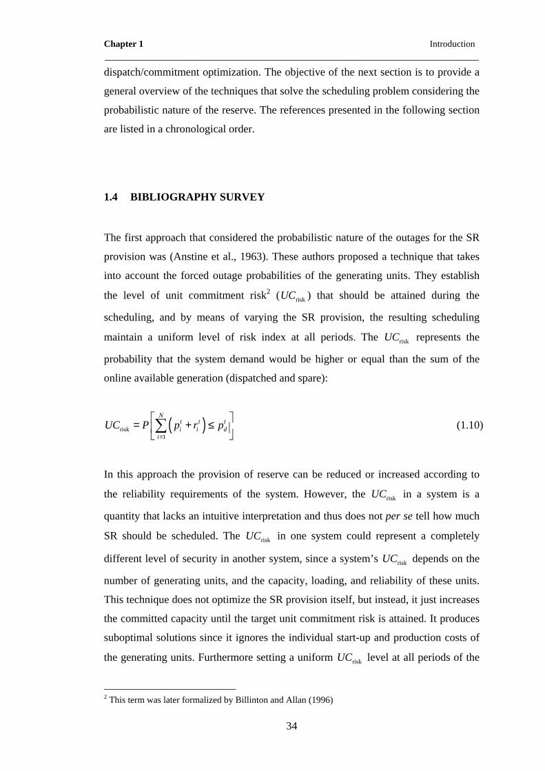
1.4 BIBLIOGRAPHY SURVEY
The first approach that considered the probabilistic nature of the outages for the SR
provision was (Anstine et al., 1963). These authors proposed a technique that takes
into account the forced outage probabilities of the generating units. They establish
the level of unit commitment risk2 ( riskUC ) that should be attained during the
scheduling, and by means of varying the SR provision, the resulting scheduling
maintain a uniform level of risk index at all periods. The riskUC represents the
probability that the system demand would be higher or equal than the sum of the
online available generation (dispatched and spare):
( )risk1
Nt t ti i d
iUC P p r p
=
= + ≤ ∑ (1.10)
In this approach the provision of reserve can be reduced or increased according to
the reliability requirements of the system. However, the riskUC in a system is a
quantity that lacks an intuitive interpretation and thus does not per se tell how much
SR should be scheduled. The riskUC in one system could represent a completely
different level of security in another system, since a system’s riskUC depends on the
number of generating units, and the capacity, loading, and reliability of these units.
This technique does not optimize the SR provision itself, but instead, it just increases
the committed capacity until the target unit commitment risk is attained. It produces
suboptimal solutions since it ignores the individual start-up and production costs of
the generating units. Furthermore setting a uniform riskUC level at all periods of the
2 This term was later formalized by Billinton and Allan (1996)
Chapter 1 Introduction ____________________________________________________________________
35
optimization horizon might be detrimental for the economic efficiency, since to
attain it at a given period might require the commitment of expensive generating
units, and such expensive reserve might not always be justified by the benefit
derived from it.
A pioneering paper on the use of integer programming for unit commitment (Dillon
et al., 1978) mentions that, in order to have a proper characterization of the reliability
level in generation scheduling, an examination of the relationship between the SR
and the risk level provided by such reserve should be performed. Another early paper
(Merlin and Sandrin, 1983) defines the marginal utility of spinning reserve as the
expected reduction in outage costs provided by the marginal MW of SR. At the
optimum, the marginal cost of SR must be equal to its marginal utility. While these
ideas were developed some time ago, it does not appear that an explicit treatment of
the value of reserve in the unit commitment problem has yet been described.
Gooi et al., (1999), appear to be the first to have considered the optimization of the
amount of reserve within the UC problem. Their approach consists in post-
processing the UC schedule to compute the level of “risk index” of consumer
disconnection at each hour. If this risk index is not within a certain range of a pre-
specified target for some periods, the SR requirement is adjusted for these periods
and the UC is run again. This method optimizes the SR provision maintaining the
UC formulation intact, but it is computationally intensive because several UC
computations may have to be performed before the target risk index is achieved.
Because a risk index level is an abstract concept that lacks an intuitively quantifiable
interpretation, they introduce another reliability metric that considers not only the
probability of having to shed load in response to a unit outage, but also consider its
extent. Then at each period an external cost/benefit analysis is used to compute the
level at which the marginal cost of SR matches the benefit it provides, i.e. the
reduction in the expected social cost of energy not supplied. It should be noted that
this approach considers the cost characteristics of generating units but ignores their
individual reliability.
The previous formulation was later extended to consider the ramp-rate limits of the
generating units in (Wu and Gooi, 1999).

Chapter 1 Introduction ____________________________________________________________________
36
In (Flynn et al., 2001) it is proposed to balance both the running cost of the system
and the expected cost of energy not served due to load curtailments. The principal
difficulty in directly representing the probabilistic nature of the outages in an
optimization problem stems from the fact that there is no direct means of
incorporating the Capacity on Outage Probability Table (COPT), (Billinton and
Allan, 1996)). In (Flynn et al., 2001), instead of computing the COPT for each
possible units combination, it is assumed that the load shed by a particular unit
outage is independent of the state of the remaining units (committed, decommitted,
synchronized or on outage). That is, it neglects possible re-dispatching of the
synchronized units to pick-up the load that the unit on outage was serving. A related,
and more serious issue is that by not using probability theory to compute the possible
states of the synchronized units (COPT), the associated expected energy not served
due to outages is inflated, and cannot be even used as a proxy. Thus, this method
overestimates the SR requirements and it results in suboptimal solutions for all cases.
Chattopadhyay and Baldick, (2002), adopt an approximation of the Loss of Load
Probability (LOLP) to quantify the risk associated with a particular schedule. This
reliability metric is approximated using an exponential function whose parameters
are system-dependent. Essentially, this function estimates the required SR in the
system to attain a given LOLPtarget. This approximation is then incorporated in the
formulation of the UC optimization problem as an extra linear constraint at each
period of the optimization horizon:
( )target1
Nt
ii
r f LOLP=
≥∑ (1.11)
Enforcing this constraint keeps the risk of disconnection below the predefined
threshold (LOLPtarget). Since the probability of disconnection is represented explicitly
in this method, post-processing of the results and iterations are avoided. On the
other hand, this approach is not self-contained because it requires the selection of an
appropriate LOLPtarget. While these authors claim that this criterion could be set
based on a cost/benefit analysis, this might be difficult because the reserve and
interruption costs depend on the generating units that are scheduled and thus change
Chapter 1 Introduction ____________________________________________________________________
37
at each period. LOLP is also not particularly suited to the computation of the societal
cost of outages because it measures only the probability that the load exceeds the
generating capacity but does not quantify the extent of the disconnections that might
result from such deficits. Setting arbitrarily the LOLPtarget would lead to generation
schedules that are not economically optimal. If a high LOLP ceiling were set, there
would regularly be insufficient reserve to cover unforeseen generation deficits.
Conversely, if this ceiling were set too low, the increase in the cost of the generation
schedule would exceed the potential economic benefits of avoiding load
disconnections.
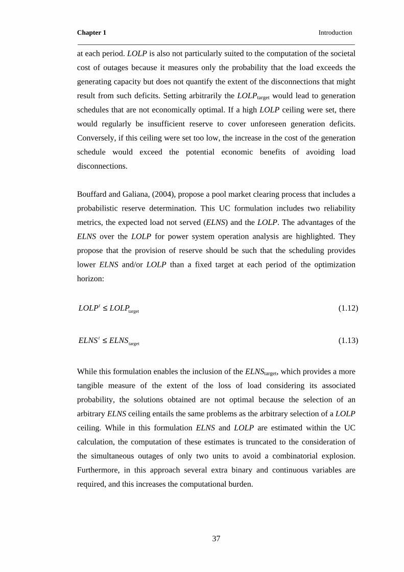
Bouffard and Galiana, (2004), propose a pool market clearing process that includes a
probabilistic reserve determination. This UC formulation includes two reliability
metrics, the expected load not served (ELNS) and the LOLP. The advantages of the
ELNS over the LOLP for power system operation analysis are highlighted. They
propose that the provision of reserve should be such that the scheduling provides
lower ELNS and/or LOLP than a fixed target at each period of the optimization
horizon:
targettLOLP LOLP≤ (1.12)
targettELNS ELNS≤ (1.13)
While this formulation enables the inclusion of the ELNStarget, which provides a more
tangible measure of the extent of the loss of load considering its associated
probability, the solutions obtained are not optimal because the selection of an
arbitrary ELNS ceiling entails the same problems as the arbitrary selection of a LOLP
ceiling. While in this formulation ELNS and LOLP are estimated within the UC
calculation, the computation of these estimates is truncated to the consideration of
the simultaneous outages of only two units to avoid a combinatorial explosion.
Furthermore, in this approach several extra binary and continuous variables are
required, and this increases the computational burden.

Chapter 1 Introduction ____________________________________________________________________
38
Wang et al., (2005) propose an independent paid-as-bid operating reserve market in
which a function that represents the social benefit/losses is maximized/minimized.
This function combines two conflicting objectives: on the one hand the cost of
reserve increases with its companion provision, on the other, the expected cost of
interruptions decreases as the provision of reserve increase. The minimization
problem on a uniform clearing price ( cleartπ ) is formulated as follows:
clear1
minRN
t t ti
iVOLL EENS rπ
=
× +
∑ (1.14)
In which NR is the set of candidate units to procure SR. The optimal amount of SR is
such that the cost matches the benefit derived from it. This process is repeated for
each of the periods of the optimization horizon. However, in this process the
individual reliability of the generating units is ignored. Furthermore, it assumes that
the reserve market is independent of the energy market, thus the bidders are limited
to be already synchronized generating units. Ignoring the coupling that exists
between the energy and the reserve scheduling can lead to suboptimal or infeasible
results, (Galiana et al., 2005).
Simultaneously to the work presented in this thesis in (Bouffard et al., 2005a) and
(Bouffard et al., 2005b) it is proposed to include the ELNS in the objective function.
By doing so, the need of imposing an ELNS ceiling is averted. Furthermore, the
difficulties in selecting ELNS limits are mentioned as well as the resulting
infeasibilities that can arise if there are insufficient reserve resources to attain such
ceiling, or if these resources are very unreliable. The formulation presented in these
papers is of a stochastic programming problem in which dimensionality problems are
present due the possible permutations of units that the optimization process might
consider. Thus the authors assume that only one contingency can occur during the
time horizon in order to consider a tractable amount of cases.

Chapter 1 Introduction ____________________________________________________________________
39
1.5 PROPOSED FORMULATIONS
In this dissertation, three approaches to overcome the problem of optimizing the
spinning reserve provision are presented.
In the first approach, the traditional reserve constraint is omitted and instead the
expected cost of outages is included in the objective function. Thus, the objective
function combines conflicting objectives that must be minimized together. On the
one hand, by increasing the spinning reserve provision the operating costs of the
system increase, while the cost of the expected energy not served (EENS) is reduced.
Conversely, by reducing the spinning reserve procurement, the operating cost of the
system is reduced and the cost of EENS increases. In this model the full EENS
distribution is included in the optimization process. Since there are no direct means
of doing so in a tractable way, the EENS distribution is computed off-line, and then
introduced as a look-up table in the UC calculation, which determines the optimal
schedule and the spinning reserve requirements. This formulation is not directly
applicable to systems of realistic size since the number of elements in the look-up
table is: 2N T× . Thus, this approach is used only to demonstrate some concepts in
Chapter 2.
As in the first approach, the second approach also considers the social cost of
outages explicitly under the form of an additional term in the objective function of
the UC problem. The optimization then automatically determines the amount of
reserve that minimizes the sum of the operating cost and the expected cost of outages
caused by failures of generating units at each period of the optimization horizon in a
single UC run. Representing explicitly the expected cost of outages is possible only
if this cost can be estimated for any combination of generating units. While this
quantity can be computed rigorously for a given combination of generating units and
a given load, repeating this calculation for all the combinations that the UC program
might consider would require a prohibitive amount of computing time. A further
contribution of this approach is thus the development of a fast yet accurate method
for estimating the EENS for any load and any combination of generating units.
Chapter 1 Introduction ____________________________________________________________________
40
In the third approach, the level of SR that minimizes the sum of the running cost of
the system and the EENS costs is calculated off-line for every period of the
scheduling horizon. This time-decoupled solution takes into consideration the
demand at each period as well as the cost and reliability characteristics of the
available units. Once this information is gathered, the SR requirements computation
problem is formulated as a bilevel optimization process in which the SR procurement
constitutes the upper level decision-making, and a single period UC forms the lower
level decision-making instance. Once the optimal SR requirements at each period of
the optimization horizon are computed, they are fed to a traditional UC formulation
in which the overall solution considering the inter-temporal couplings of the
generating units are considered. A clear advantage of this approach is that it keeps
the UC formulation intact, and thus its applicability is straightforward to any system
of any size.
In general, these approaches avoid several problems, such as the need to select the
risk level on the basis of an exogenous cost/benefit analyses, the need to iterate the
UC solution, the need for post-processing the results and the arbitrary selection of
risk targets for each optimization period. The proposed models assume that random
outages of generating units are the only source of uncertainty. Errors in the load
forecast and the effect of the transmission and distribution networks are not taken
into account. It also assumes that the disturbances do not extend beyond the
optimization period during which they occur. These techniques are organized and
presented as described in the following section.
1.6 OUTLINE OF THE THESIS
Chapter 2: Traditional and Proposed Unit Commitment
In this chapter the mathematical formulation of the primal UC problem is presented.
In this chapter, it is also proposed a UC formulation that includes the full EENS
distribution, which has been computed off-line and integrated as a look-up table into
the optimization process. In a similar way, a third UC approach that includes the full

Chapter 1 Introduction ____________________________________________________________________
41
LOLP probability distribution is presented. Comparisons among these techniques are
performed on a three-unit system.
Chapter 3: Optimal Scheduling of Spinning Reserve Considering the Cost of
Interruptions
This chapter presents a new technique that modifies the UC in order to optimize the
sum of the operating costs and the expected costs of energy not served. In this
chapter a novel and fast method to estimate the EENS for any combination of units is
also presented. This approximation is then embedded in the optimization process.
Chapter 4: Optimal Scheduling of Spinning Reserve Considering the Failure to
Synchronize by EENS proxies
This chapter presents an extension of the proposed UC formulation of Chapter 3. A
three-state reliability model of the generating units is presented and validated by
Monte Carlo methods. This model in then included in the optimization process by
proxies. This UC approach takes into account not only random outages, but also of
the failures of cycling and peaking units to synchronize.
Chapter 5: Optimizing the Spinning Reserve Requirements
In this chapter a new technique that optimizes the SR requirements for each period of
the optimization horizon prior to the UC calculation is presented. These SR
requirements are then enforced at each period of the optimization horizon using the
traditional reserve constraint, keeping the UC formulation intact.
Chapter 6: Economic Impact Assessment of Load Forecast Errors in the
Operation of the Power System
In this chapter the economic impact of the load forecast errors are assessed. This
study shows that, in order to have a more realistic estimate of the economic impact
of load forecast errors on the daily power system operation; the cost of expected
energy not served must be taken into account.
Chapter 7: Conclusions and Suggestions for Further Work
Chapter 7 summarizes the main achievements of this investigation. It also suggests
further work.

Chapter 1 Introduction ____________________________________________________________________
42
Appendices
A number of appendices complement the present thesis. Appendix A presents the
basic principles of contingencies probability calculation. Appendix B presents the
data of the test systems used in this thesis. Appendix C presents the Mixed Integer
Linear Programming formulation of the traditional Unit Commitment and the data
for the three-segments the piecewise linear approximation of the production cost
functions of the generating units.

Chapter 2 Traditional and Proposed Unit Commitment ____________________________________________________________________
43
Chapter 2
Traditional and Proposed Unit Commitment
2.1 INTRODUCTION
The demand for electrical energy has a daily and weekly cyclic nature that follows
the pattern of human activities. Meeting this electrical demand at a minimum cost
while keeping the system secure is a difficult challenge that the utilities and power
system operators have to face. This short-term optimization problem consists in
scheduling the generator start-ups, shut-downs and determine their production levels
to meet the short-term forecasted demand. Its purpose is to minimise the production
and start-up/shut-down costs across all the generating units and over the optimization
horizon (24 or at most 168 hours) while satisfying all the operating constraints.
The process of deciding when and which generating units at each power station to
start-up and shut-down, while deciding the individual power outputs of the
scheduled units and maintaining a given level of spinning reserve at each time period
is called Unit Commitment (UC). Committing and dispatching the units in a power
system is a challenging optimization problem because of the large number of
possible combinations of units at each of the time periods in the optimization
horizon. Thus, unit commitment is a complex optimization problem that mixes
binary and continuous variables. The non-linearity of the cost functions and of the
start-up cost increases the complexity of the problem.
The following section presents a generic unit commitment formulation along with
the most relevant constraints.

Chapter 2 Traditional and Proposed Unit Commitment ____________________________________________________________________
44
2.2 UNIT COMMITMENT FORMULATION
2.2.1 Objective Function
The Unit Commitment (UC) problems consist in determining the generating units
that need to be committed and their production levels to supply the forecasted short
term demand and spinning reserve (SR) requirements at a minimum cost, (Wood and
Wollenberg, 1996, Baldick, 1995, Padhy, 2004). The operation of these units is
subject to several constraints. UC problems are large nonlinear mixed-integer
programming problems.
The primal UC problem is formulated as follows:
( ) ( )1 1
min ,T N
t t t ti i i i i
t ic u p s u
= =
+ ∑∑ (2.1)
Where:
( ),t ti i ic u p : power production cost of unit i during period t
( )t ti is u : cost of a possible start-up of unit i during period t
tip : power produced by unit i during period t
tiu : status of unit i during period t , (1: committed, 0: decommitted)
T : number of periods in the optimization horizon
N : number of available generating units
It should be noted that due to the introduction of the binary variable tiu , the UC
problem is not convex.
2.2.2 Cost Function
The production cost of a thermal generating unit is often a nonconvex function, but
these functions are usually approximated by convex quadratic functions in the
economic dispatch and UC solution algorithms, (Wood and Wollenberg, 1996,

Chapter 2 Traditional and Proposed Unit Commitment ____________________________________________________________________
45
Madrigal and Quintana, 2000). Therefore the production cost of generating unit i is
modelled as:
( ) ( )2,t t t t t
i i i i i i i i ic u p u a p b p c = + + (2.2)
A piecewise linear approximation of this function is presented in Appendix C.
2.2.3 Start-up Cost
The start-up cost of a thermal unit is a function of the time the unit has been shut
down. That is, it is cheaper to restart a warm generating unit, that a cold one. This
effect is usually approximated by exponential
( ) ( )off
11 1i
i
tt t t ti i i i i is u u u e ζκ ρ−
= − − −
(2.3)
In the previous equation, offit stands for the number of hours that a unit has been
decommitted up to period 1t − . iκ is the fixed cost of bringing online the generating
unit i ; this cost includes the crew expense and maintenance expense. iρ is the cold
start-up fuel cost of unit i and iζ is the thermal time constant of unit i . However, for
the sake of simplicity, the start-up costs can be considered constant for each unit
being synchronized with the system; thus, the start-up cost of generating unit i
during period t :
( ) ( )11t t t ti i i i is u u uκ −= − (2.4)
At 1t = , the start-up cost would depend on the history of the unit ( 0iu ), that is, if
0 1iu = , then the start-up cost is zero, since the unit was already committed in the
previous period. On the other hand, if 0 0iu = then the start up cost is iκ .

Chapter 2 Traditional and Proposed Unit Commitment ____________________________________________________________________
46
2.2.4 Power Balance
At each period, the solution must be such that the total generation matches the
system demand ( tdp ):
10
Nt t td i i
ip u p
=
− =∑ (2.5)
2.2.5 Spinning Reserve Requirement
To ensure that the schedule provides at least the required amount of SR ( tdr ) during
period t , UC programs enforce the following constraint:
10
Nt t
d ii
r r=
− ≤∑ (2.6)
Where tir is the contribution that unit i makes to the SR during period t . This
contribution is given by:
( ) ( ){ }max upmin ,t t t ti i i i i ir u P p u Rτ= − (2.7)
In which upiR is the ramp-up rate of unit i and τ is the amount of time available for
the generators to ramp-up their output to deliver the reserve generation.
2.2.6 Power Output Limits
Besides the power balance constraint and the reserve constraint, each of the thermal
generating units is subject to its own operating constraints. Among these the
minimum and maximum production levels ( maxiP and min
iP respectively) for unit i at
period t are such that:
min mint t t
i i i i iu P p u P≤ ≤ (2.8)

Chapter 2 Traditional and Proposed Unit Commitment ____________________________________________________________________
47
2.2.7 Minimum-up and -down Time
These constraints state that the time a unit has been committed (decommitted),
before it can be decommitted (committed), has to be greater than or equal to a
required minimum time upit ( dn
it ).
The minimum up-time constraints for unit i are given by:
up H up H1 1, , , 0m
i i i i iu m t t t t = ∀ ∈ − > > … (2.9)
{ }up
1 1
1 2
min 1,1 i
t t ti i it t ti i i
t t Tt ti i i
u u uu u u
u u u
− +
− +
+ −−
− ≤
− ≤
− ≤
" 2,3, , 1t T∀ = −… (2.10)
Where upit is the minimum number of periods the unit has to be committed. The
minimum down-time constraints of unit i are given by:
dn H dn H0 1, , , 0m
i i i i iu m t t t t = ∀ ∈ + − < < … (2.11)
{ }dn
1 1
1 2
min 1,1
1
1
1 i
t t ti i it t ti i i
t t Tt ti i i
u u uu u u
u u u
− +
− +
+ −−
− ≤ −
− ≤ −
− ≤ −
" 2,3, , 1t T∀ = −… (2.12)
Where dnit denotes the minimum number of periods the unit has to be down. H
it
denotes the number of periods in which generating unit i was committed or
decommitted, up to 0t = depending on the sign.
2.2.8 Ramp-up and -down Limits
A thermal generating unit has a limited ability to change its output from one level of
power production to another during a period of time. This restriction arises from

Chapter 2 Traditional and Proposed Unit Commitment ____________________________________________________________________
48
thermal and mechanical limitations. The minimum ramp-up and ramp-down
constraints include this limitation into the UC formulation. As generation increases,
these constraints are given by:
1 upt t
i i ip p R−− ≤ (2.13)
As generation decreases the constraints are given by:
1 dnt t
i i ip p R− − ≤ (2.14)
The ramp-rate limits must also be considered at the moment the unit is starting-up
and shutting down, (Wang and Shahidehpour, 1993).
All the presented constraints must be met at all periods of the optimization horizon.
All the parameters of the units are obtained from designers and field experiments.
The system requirements are set by each system operator based on standards
previously defined and tailored for each system to reach an acceptable level of risk.
A Mixed Integer Linear Programming (MILP) formulation of the presented UC
formulation can be found in Appendix C.
It must be noted that the traditional UC formulation does not integrate the reliability
impact in the reserve scheduling. As pointed out in Chapter 1, in order to optimally
set these requirements the SR marginal cost must match the marginal benefit derived
from it, which is measured in terms of reduction of the expected cost of outages.
Since the outages are random by nature, in order to make this cost/benefit analysis it
is necessary to include the full outage probability distribution within the optimization
process. The next section deals with a theoretical approach that incorporates the full
outage probability distribution in the UC calculation and thus finds the optimal
scheduling considering probabilistic reserve.

Chapter 2 Traditional and Proposed Unit Commitment ____________________________________________________________________
49
2.3 PROPOSED THEORETICAL UC APPROACH
In order to achieve the minimum overall cost of operating the system it is necessary
to include the full outage probability distribution within the UC computation for
each of the possible combinations of units. However, this is not a trivial task, since
the main problem of the probabilistic spinning reserve procurement stems from the
fact that there is no direct means of including this outage distribution in the
optimization process. Furthermore, for each possible combination of units that the
UC program might consider a Capacity on Outage Probability Table (COPT)
computation is required, Appendix A. While this quantity can be computed
rigorously for a given combination of generating units and a given load, repeating
this calculation for all the combinations that the UC program might consider would
require a prohibitive amount of computing time.
A related issue is that in order to obtain an estimate of the load and/or energy that
would not be supplied due to generating unit outages the ramp rates of the different
generating units must be considered. The ramp rates of the generating unit will limit
the spare generating capacity available to pick up load in case of a contingency.
Thus, the dispatch of the generating units will play a key role in the allocation of the
spinning reserve among the units, and as a consequence on the expected energy not
served due to outages.
This section presents a UC model that includes the full outage probability
distribution in the UC calculation.
2.3.1 Proposed Objective Function
The proposed UC formulation minimizes the following objective function:
( ) ( ) ( )1 1
min ,T N
t t t t ti i i i i LS
t ic u p s u E c
= =
+ + ∑ ∑ (2.15)
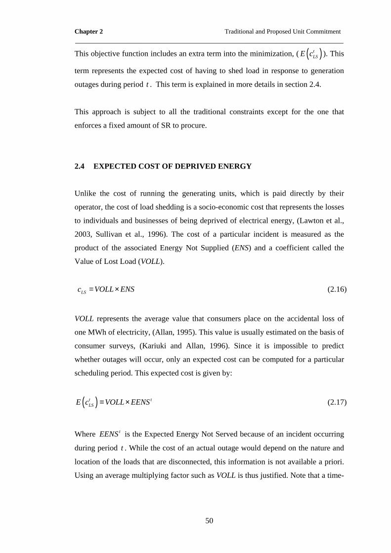
Chapter 2 Traditional and Proposed Unit Commitment ____________________________________________________________________
50
This objective function includes an extra term into the minimization, ( ( )tLSE c ). This
term represents the expected cost of having to shed load in response to generation
outages during period t . This term is explained in more details in section 2.4.
This approach is subject to all the traditional constraints except for the one that
enforces a fixed amount of SR to procure.
2.4 EXPECTED COST OF DEPRIVED ENERGY
Unlike the cost of running the generating units, which is paid directly by their
operator, the cost of load shedding is a socio-economic cost that represents the losses
to individuals and businesses of being deprived of electrical energy, (Lawton et al.,
2003, Sullivan et al., 1996). The cost of a particular incident is measured as the
product of the associated Energy Not Supplied (ENS) and a coefficient called the
Value of Lost Load (VOLL).
LSc VOLL ENS= × (2.16)
VOLL represents the average value that consumers place on the accidental loss of
one MWh of electricity, (Allan, 1995). This value is usually estimated on the basis of
consumer surveys, (Kariuki and Allan, 1996). Since it is impossible to predict
whether outages will occur, only an expected cost can be computed for a particular
scheduling period. This expected cost is given by:
( )t tLSE c VOLL EENS= × (2.17)
Where tEENS is the Expected Energy Not Served because of an incident occurring
during period t . While the cost of an actual outage would depend on the nature and
location of the loads that are disconnected, this information is not available a priori.
Using an average multiplying factor such as VOLL is thus justified. Note that a time-

Chapter 2 Traditional and Proposed Unit Commitment ____________________________________________________________________
51
dependent tVOLL could easily be incorporated in this formulation if this data were to
become available.
Determining a priori the energy that would not be served because of a particular
disturbance is very difficult because this quantity depends on the circumstances.
However, a standard technique for computing the EENS is described in (Billinton
and Allan, 1996). This technique takes into account the following factors:
• the generating units connected to the system at period t
• the probability of forced outage of each generating unit
• the amount of spinning reserve that these units can provide
• the load during period t
To keep the computation of the EENS tractable, this technique ignores any effects
that the transmission and distribution networks might have and assumes that the
effects that a disturbance might cause do not extend beyond the scheduling period
during which it occurs. In the following, this period will be taken to be one hour. To
compute the EENS a Capacity on Outage Probability Table (COPT) is generated,
(Appendix A). Given a set of generating units synchronized at the beginning of a
scheduling period, the COPT gives the probability that the total capacity on outage
during this period will be greater than or equal to a certain value. Using these
cumulative probabilities, it is then possible to calculate the probability that a certain
amount of load cannot be served because the capacity on outage exceeds the
spinning reserve. Summing the product of these probabilities with the associated
energy curtailed over all the possible outages gives the EENS for this combination of
generating units and this load level.
2.5 IMPLEMENTATION OF THE PROPOSED APPROACH
The key to implement the complete formulation as shown in equation (2.15) is the
inclusion of the full outage distribution within the optimization program (UC). For
system of realistic size this is simply not feasible, because the number of

Chapter 2 Traditional and Proposed Unit Commitment ____________________________________________________________________
52
permutations of units that the UC program might consider is much too large. In this
section a theoretical approach is proposed. In this approach the outage distribution is
computed offline and then included within the optimization process. Consider for
instance the system shown in Figure 2.1.
P1max = 100 MW
P2max = 100 MW
ptd
P3max = 100 MW
ut1
ut2
ut3
P1max = 100 MW
P2max = 100 MW
ptd
P3max = 100 MW
ut1
ut2
ut3
Figure 2.1 Three-unit system
The system shown in Figure 2.1 consists of 3 generating units of equal capacity and
the data of these units is shown in Table 2.1. In this table miniP and max
iP are the
minimum and maximum generating limits of unit i respectively. ai, bi, and ci are the
coefficients of the cost function of unit i and ORRi is the outage replacement rate of
unit i , (Billinton and Allan, 1996).
Table 2.1 Three-unit system
i Unit Pimin Pi
max ai,
($/MW2h)
bi,
($/MWh)
ci,
($/h)
ORR
1 U1 25.0 100.0 0.00623 18 217.895 0.010
2 U2 25.0 100.0 0.00612 18.1 218.335 0.005
3 U3 25.0 100.0 0.00598 18.2 218.775 0.001
For the sake of simplicity, at this point it is considered a single time period during
which these units must supply a load of 90 MW. Since this system consists of three
units, there are 23 possible combinations of units. Neglecting the ramp rates of the
generating units the EENS of each these combinations is shown in Table 2.2.

Chapter 2 Traditional and Proposed Unit Commitment ____________________________________________________________________
53
Table 2.2 Commitment status and associated EENS, L = 90 MW
Commitment Number
(Dt) U1 U2 U3
EENS
(MWh)
1 0 0 0 90.00
2 1 0 0 0.90
3 0 1 0 0.45
4 1 1 0 0.0045
5 0 0 1 0.09
6 1 0 1 0.00090
7 0 1 1 0.00045
8 1 1 1 4.5×10⁻⁶
Table 2.2 shows that each possible combination of units is enumerated. This decimal
representation of the combination of units at period t is the variable tD . Even once
the full outage probability distribution has been obtained for the system and a
particular load, it does not seem to be possible to obtain an accurate analytical
function to approximate it. To overcome this problem each of these values can be
included into the optimization process by means of enforcing the following
constraints:
1
12 1
Ni t t
ii
u D−
=
+ =∑ (2.18)
2
1
N
t tk
kk Dλ
=
=∑ (2.19)
2
11
N
tk
kλ
=
=∑ (2.20)
( )2
1
N
t t tLS k k
kE c VOLL EENS λ
=
= ∑ (2.21)

Chapter 2 Traditional and Proposed Unit Commitment ____________________________________________________________________
54
Where tkλ is a binary variable, ( [ ]0,1t
kλ ∈ ). The variable tiu determines whether unit
i is committed at period t . These constraints model an explicit exhaustive
enumeration through binary variables. Suppose that units U2 and U3 are committed.
In this case equation (2.18) shows that the decimal representation for this
commitment is 7tD = , (Table 2.2). Once the value of tD is obtained, equation
(2.19) enumerates all the possible commitment scenarios, and the one corresponding
to tD is enabled by the variable tkλ . It should be noted that several combinations of
tkλ can trigger the same value of tD due the coefficients k ; e.g.
2 52 5 7t tλ λ+ = , 1 66 7t tλ λ+ = , 3 43 4 7t tλ λ+ = , 1 2 42 4 7t t tλ λ λ+ + = , etc. Thus, it is
required to restrict that only one of all the possible scenarios is selected. Enforcing
constraint (2.20) assures that a single tkλ can be selected at each period, (i.e. 7 1tλ = ).
By doing so, equation (2.21) reduces to (2.17) with the appropriate value of EENS
for a given commitment.
2.5.1 Spinning Reserve Requirements, Units’ Scheduling and VOLL
In the traditional UC formulation the spinning reserve requirements are set
deterministically. Units are committed and loaded solely according to their marginal
cost of production. The marginal cost of production of unit i is given by, (Stoft,
2002, Kirschen and Strbac, 2004):
( ) ( )tit
i i ti
d c pMC p
dp= (2.22)
Then, from Table 2.1 it can be appreciated that the unit with the lower marginal cost
is unit U1 followed by U2 and finally by U3. Thus, this is the expected loading order
of the units as the load and/or spinning reserve requirements increase. Figure 2.2
shows the single period scheduling for different spinning reserve requirements.

Chapter 2 Traditional and Proposed Unit Commitment ____________________________________________________________________
55
0 10 30 60 90 110 130 150 180 210
1
2
3
Spinning reserve requirements, MWU
nit
Figure 2.2 Scheduling as a function of the spinning reserve requirements
Figure 2.2 shows that, as the spinning reserve requirements increase; the units are
committed according to their marginal cost. This scheduling is insensitive to the
VOLL; hence, enough capacity is committed until the demand and the spinning
reserve requirements are fulfilled. For all cases, unit U1, which is the one with the
lowest marginal cost is committed. The second cheapest unit is unit U2, then as the
spinning reserve requirements increase, unit U2 starts being committed. If the
spinning reserve requirements continue increasing the UC program commits all of
the available units.
Setting the spinning reserve requirements using deterministic techniques and
ignoring their individual reliability hinders the ability of the optimization process to
reach the overall optimum. If instead of using the traditional UC the proposed
formulation in which the constraints that include the full outage probability
distribution are considered is used, then, the scheduling and thus the spinning reserve
provision will be function of the reliability of the generating units and the system
VOLL.
101 102 103 104
1
2
3
VOLL, $/MWh
Uni
t
Figure 2.3 Scheduling as a function of the VOLL, proposed approach
Chapter 2 Traditional and Proposed Unit Commitment ____________________________________________________________________
56
Figure 2.3 shows that for low VOLLs the first selection of this UC formulation is the
cheapest unit. Table 2.1 shows that the unit with the lower marginal cost is also the
less reliable. Thus as the VOLL increases (and thus the expected cost of energy not
served) instead of committing a second unit, the program changes to a more
expensive but also more reliable generating unit (unit U2). The same happens with
unit U3, which has the largest marginal cost of production but which is also the most
reliable. If the VOLL continues increasing the proposed UC formulation commits
two units, the first selection being the cheapest combination. As the VOLL continues
to increase, the set of units selected becomes more expensive but also more reliable.
It should be noted that committing all of the units is not justified even for entirely
large VOLLs.
Both the traditional and the proposed approaches can procure the same amount of
spinning reserve. However, enforcing the traditional reserve constraint reduces
significantly the possible combinations of units in order to achieve a lower EENS for
the same amount of reserve. For instance, the traditional approach commits units U1
and U2 to procure 110 MW of SR. Thus the EENS for this combination is 0.0045
MWh. On the other hand, the proposed approach can provide the same amount of SR
with different levels of risk, just by selecting different combinations of units (i.e.
with EENS equal to 0.0045, 0.00090 or 0.00045 MWh depending on the
combination of units and VOLL). By doing this, the running cost of the system
increases but at the same time the expected cost of outages reduced.
2.5.2 Optimal Scheduling and Load Variations
The previous section showed the sensitivity of the optimal scheduling to the VOLL.
The optimal amount of SR is function not only of the VOLL but also of the load level
to serve. Figure 2.4 shows the effect of the load level for two different values of
VOLL.

Chapter 2 Traditional and Proposed Unit Commitment ____________________________________________________________________
57
20 40 60 80 100 120 140 160 180 200
1
2
3
Load, MW
Uni
t
20 40 60 80 100 120 140 160 180 200
1
2
3
Load, MWU
nit
VOLL = 2000 $/MWh
VOLL = 6000 $/MWh
Figure 2.4 Scheduling as a function of the load level
As expected, when the VOLL is low, the amount of SR is low, as the VOLL increases
the SR procurement increases. This figure shows also that as the load level increases
the optimal scheduling changes, committing more units. Figure 2.5 shows that for
larger VOLLs the proposed formulation will tend to commit more capacity to reduce
the EENS. This extra commitment of generating units is associated with an
increment in the dispatch cost; however, the “savings” derived from the EENS cost
reduction justifies this cost increment.
40 60 80 100 120 140 160 180100
101
102
103
Load, MW
EE
NS
cos
t, $
40 60 80 100 120 140 160 1800
1000
2000
3000
4000
Load, MW
disp
atch
cos
t, $
VOLL = 2000 $/MWhVOLL = 6000 $/MWh
VOLL = 2000 $/MWhVOLL = 6000 $/MWh
Figure 2.5 EENS and dispatch costs for the different VOLLs

Chapter 2 Traditional and Proposed Unit Commitment ____________________________________________________________________
58
It should be noted that in the proposed formulation the spinning reserve procurement
is not explicit. That is, there is no constraint that limits the minimum or maximum
amount of this resource. On the other hand, its procurement is such, that it minimizes
the EENS and running cost simultaneously. For instance, for a VOLL of 2,000
$/MWh and a load level of 99 MW units 1 and 3 are committed, and thus the SR
provided is 101 MW. If the load increases to 114 MW units 3 and 2 are committed.
The SR provided is then 86 MW. However the two most reliable units are committed
and thus the EENS cost reduced. Figure 2.6 shows the SR procurement as a function
of the load level for the assumed VOLLs.
40 60 80 100 120 140 160 1800
50
100
150
200
Load, MW
Spi
nnin
g R
eser
ve, M
W
VOLL = 2000 $/MWhVOLL = 6000 $/MWh
Figure 2.6 Spinning reserve provision as a function of the load level
2.5.3 Optimal Scheduling and LOLP
If no SR requirements were set, and the three-unit system is to serve a load of 90
MW with a VOLL of 6,000 $/MWh, then the optimal scheduling can be obtained by
means of considering each of the possible combinations of units, Table 2.3.
Table 2.3 Optimal scheduling, three-unit system, L = 90 MW and VOLL = 6,000 $/MWh
Scheduling
U1 U2 U3
Running
cost, $
EENS
cost, $
Total
cost, $
LOLP
0 0 0 0 540000 540000 1
1 0 0 1889.28 5400 7289.3 0.01
0 1 0 1897.83 2700 4597.8 0.005
1 1 0 2086.51 27 2113.5 5×10⁻⁵
0 0 1 1906.10 540 2446.1 0.001
1 0 1 2090.69 5.4 2096.1 1×10⁻⁵

Chapter 2 Traditional and Proposed Unit Commitment ____________________________________________________________________
59
0 1 1 2095.87 2.7 2098.6 5×10⁻⁶
1 1 1 2300.96 0.027 2301.0 5×10⁻⁸
From Table 2.3 it can be appreciated that the proposed approach minimizes an
objective function that combines conflicting objectives. On the one hand, scheduling
as few units as possible and selecting those with the lowest marginal cost of
production minimizes the running cost of the system. On the other hand, by doing so
the expected cost of the outages is increased. The optimum minimizes both
objectives simultaneously.
This table also shows the associated LOLP for each scheduling. The LOLP does not
per se tell how much SR should be scheduled. Furthermore, for equal amounts of SR
there could be associated different values of LOLP. LOLP is not particularly suited
for operation purposes, since it measures the probability that, in case of a
contingency, the load to serve exceeds the available capacity; however, does not
consider the extent of the contingency.
It is possible to include the full LOLP distribution in the optimization process in a
similar way as the EENS by using the objective function of the traditional UC
formulation (equation (2.1)), replacing equation (2.21) by:
2
1
N
t t tk k
kLOLP LOLP λ
=
=∑ (2.23)
Where tkLOLP represents the loss of load probability at period t of the kth
combination of units. An extra constraint of the following form must be enforced:
targettLOLP LOLP≤ (2.24)
This formulation commits the units as shown in Figure 2.7 depending on the
targetLOLP ; however the question: “What is the optimal targetLOLP ?”, does not have
an easy answer. Since the LOLP does not take into account the severity of the

Chapter 2 Traditional and Proposed Unit Commitment ____________________________________________________________________
60
contingencies an exogenous cost/benefit analysis is required to set an appropriate
value. In the external cost/benefit analysis a reliability metric that takes into account
the likeliness and severity of the contingency (i.e. EENS or ELNS) is required. To
compute this metric, a COPT calculation for each candidate set of generating units is
needed. This results in extra computational burden.
10-8 10-7 10-6 10-5 10-4 10-3 10-2
1
2
3
LOLPtarget
Uni
t
Figure 2.7 Scheduling as a function of LOLPtarget
A related and more serious issue is that the LOLP is clearly a function of the load to
be served, of the units committed and of their individual reliability. The optimal
targetLOLP thus changes form one period of the optimization horizon to another. For
instance, Table 2.3 shows that for a load of 90 MW with VOLL = 6,000 $/MWh the
targetLOLP should be 1×10⁻⁵ in the three-unit system. This is because setting this
value as a target will yield the optimum cost in the scheduling. However if the
demand is 106 MW then the targetLOLP is obtained from Table 2.4:
Table 2.4 Optimal scheduling, three-unit system, L = 106 MW and VOLL = 6,000 $/MWh
Scheduling
U1 U2 U3
Running
cost, $
EENS
cost, $
Total
cost, $
LOLP
0 0 0 0 636000 636000 1
1 0 0 2080.2 42000 44080 1
0 1 0 2089.5 39000 41090 1
1 1 0 2384.77 568.2 2952.97 0.01495
0 0 1 2098.6 36600 38699 1
1 0 1 2389.84 401.64 2791.48 0.01099
0 1 1 2395.54 218.82 2614.36 0.005995
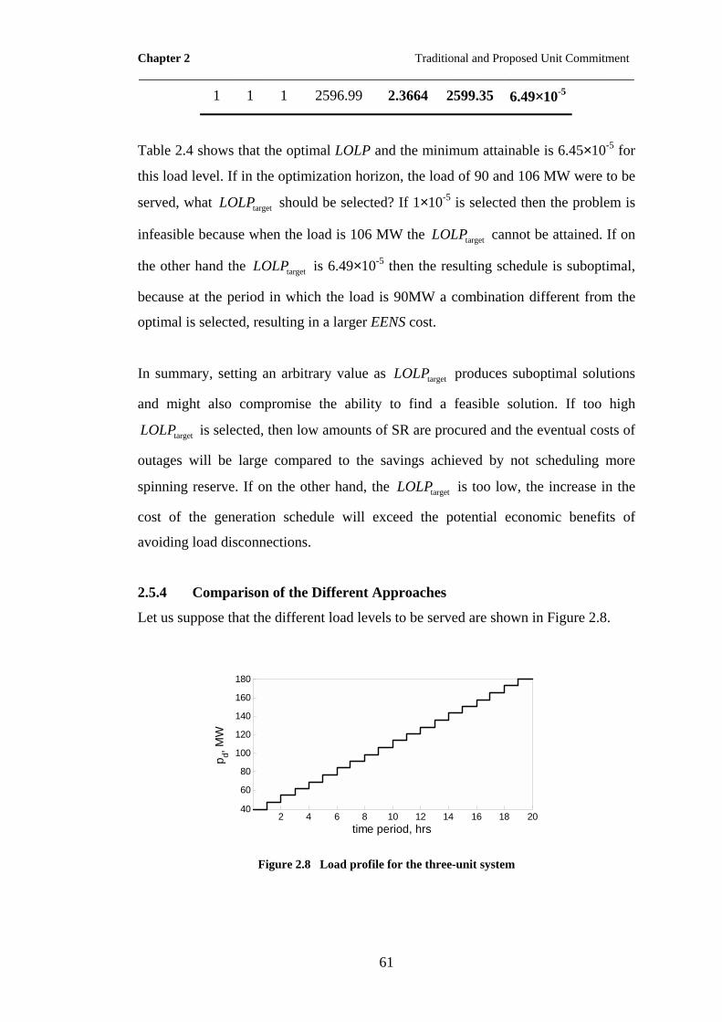
Chapter 2 Traditional and Proposed Unit Commitment ____________________________________________________________________
61
1 1 1 2596.99 2.3664 2599.35 6.49×10⁻⁵
Table 2.4 shows that the optimal LOLP and the minimum attainable is 6.45×10⁻⁵ for
this load level. If in the optimization horizon, the load of 90 and 106 MW were to be
served, what targetLOLP should be selected? If 1×10⁻⁵ is selected then the problem is
infeasible because when the load is 106 MW the targetLOLP cannot be attained. If on
the other hand the targetLOLP is 6.49×10⁻⁵ then the resulting schedule is suboptimal,
because at the period in which the load is 90MW a combination different from the
optimal is selected, resulting in a larger EENS cost.
In summary, setting an arbitrary value as targetLOLP produces suboptimal solutions
and might also compromise the ability to find a feasible solution. If too high
targetLOLP is selected, then low amounts of SR are procured and the eventual costs of
outages will be large compared to the savings achieved by not scheduling more
spinning reserve. If on the other hand, the targetLOLP is too low, the increase in the
cost of the generation schedule will exceed the potential economic benefits of
avoiding load disconnections.
2.5.4 Comparison of the Different Approaches
Let us suppose that the different load levels to be served are shown in Figure 2.8.
2 4 6 8 10 12 14 16 18 2040
60
80
100
120
140
160
180
time period, hrs
p d, MW
Figure 2.8 Load profile for the three-unit system

Chapter 2 Traditional and Proposed Unit Commitment ____________________________________________________________________
62
Figure 2.9 shows the UC solutions for the traditional formulation with
( )maxmaxt td i ir u P= , the proposed formulation with a VOLL = 6,000 $/MWh and the
formulation that includes the full LOLP distribution with 3target 1 10LOLP −= × . The
targetLOLP has been selected large, because for heavy loads the optimal is 6.49×10⁻⁵,
however to attain this target for light loads more than one unit must be committed.
However, due to the minimum production levels of the generating units, this is not
possible. This further demonstrates the limitations of selecting LOLP or ELNS
targets. Something similar happens with the traditional UC formulation. For
instance, for light loads (e.g. 40 MW) since all the units have a minimum stable
generation of 25 MW and a maximum generation of 100 MW, it is not possible to
serve the load with two units committed. On the other hand, if only one unit is
committed, the reserve constraint is violated. Thus for this period a different criterion
should be selected in order to avert infeasibility.
2 4 6 8 10 12 14 16 18 20
1
2
3
2 4 6 8 10 12 14 16 18 20
1
2
3
Uni
t
2 4 6 8 10 12 14 16 18 20
1
2
3
time period, hrs
Traditional
Modified O.F., includingEENS distribution
LOLPtarget to attain
Figure 2.9 Scheduling for each approach
Figure 2.9 shows the schedules for each of the approaches considered. Note that at
period 1 and 2 for the traditional UC approach tdr is set to 60 and 53 MW
respectively in order to avert infeasibility. Figure 2.10 shows the spinning reserve
provision with each of these approaches.

Chapter 2 Traditional and Proposed Unit Commitment ____________________________________________________________________
63
0 2 4 6 8 10 12 14 16 18 200
20
40
60
80
100
120
140
160
180
200
time period, hrs
Spin
ning
rese
rve,
MW
TraditionalModified O.F.LOLPtarget
Figure 2.10 Spinning reserve provision with different UC approaches
Figure 2.10 shows that the traditional approach and the proposed approach that
includes the cost of the outages in the objective function schedule the same amount
of spinning reserve, even though they produce different UC solutions (that is the
reason why they are overlapped and the dotted line cannot be seen). This is because
the capacity of the generating units is the same, and the overall capacity committed
at each period with both formulations is the same. On the other hand, the approach
that enforces a single target LOLP to be met at all periods produced a solution with
low amounts of SR at some periods. This is because of the large targetLOLP selected.
Enforcing a lower risk limit causes the problem to be infeasible.

Chapter 2 Traditional and Proposed Unit Commitment ____________________________________________________________________
64
0 2 4 6 8 10 12 14 16 18 200
1000
2000
3000
4000
time period, hrs
disp
atch
cos
t, $
0 2 4 6 8 10 12 14 16 18 20100
101
102
103
104
time period, hrsE
EN
S c
ost,
$
TraditionalModified O.F.LOLPtarget
TraditionalModified O.F.LOLPtarget
Figure 2.11 Itemized costs for each UC approach
Figure 2.11 shows the itemized costs for each UC approach at each period of the
optimization horizon. In the first two periods of the optimization horizon, the
spinning reserve requirements in the traditional UC approach have been reduced in
order to avert infeasibility. By doing so, the traditional UC approach commits the
unit that has the lowest marginal cost, which happens to be the less reliable one and
this is mirrored as an increase in the EENS cost. For the remaining periods both, the
traditional approach and the proposed approach with the modified objective function
schedule the same amount of SR; however, it can be appreciated that the EENS cost
in the proposed approach is lower since the proposed approach selects the most
reliable units to minimize the overall costs. On the other hand, the approach that
includes the full LOLP distribution commits enough units until the target is attained.
Since this target is not optimal for all periods, the EENS is higher than what is
achieved with the proposed approach. It could be argued that the approach that
includes the LOLP distribution produces a larger EENS costs, but a significant
reduction on the dispatch costs; however this is not the lowest overall cost, as shown
in Table 2.5.
Table 2.5 shows that the proposed approach is also the cheapest compared to the
other UC approaches. Comparing the proposed approach with the traditional
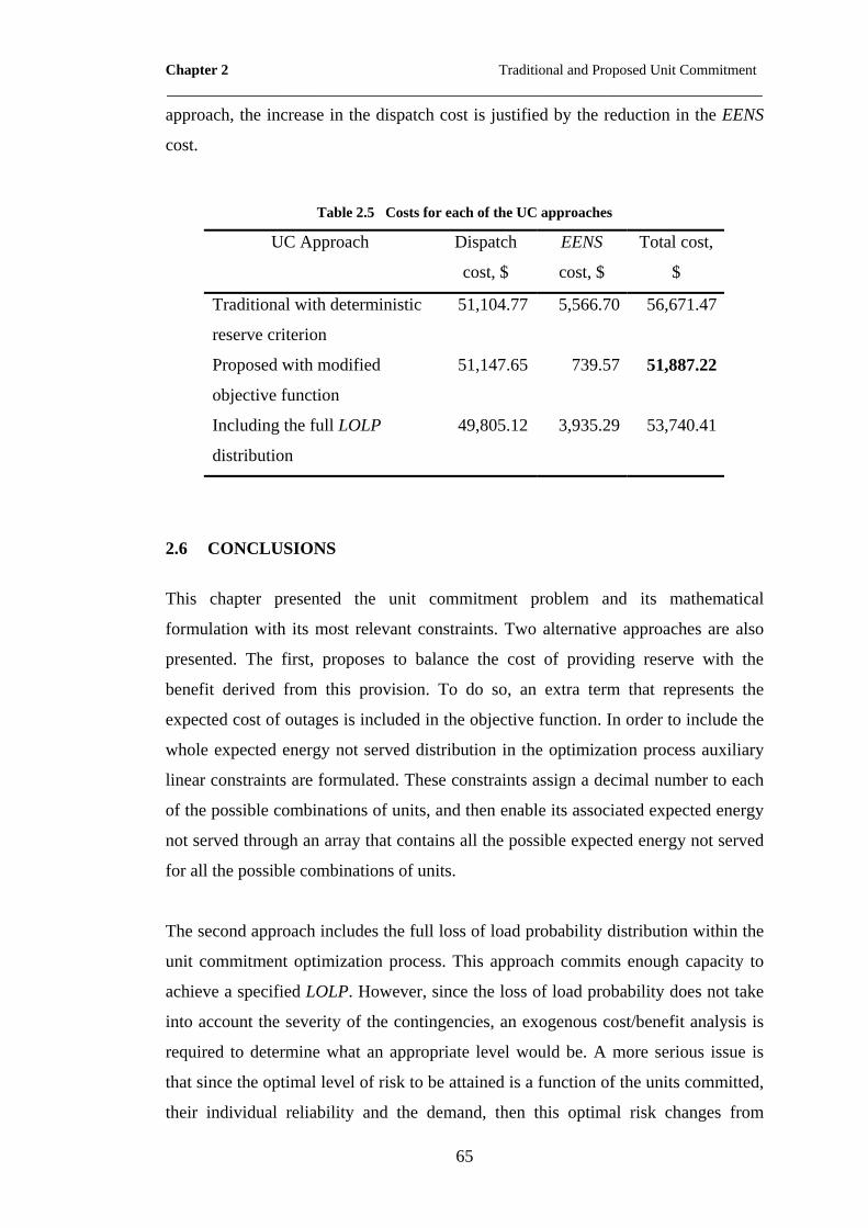
Chapter 2 Traditional and Proposed Unit Commitment ____________________________________________________________________
65
approach, the increase in the dispatch cost is justified by the reduction in the EENS
cost.
Table 2.5 Costs for each of the UC approaches
UC Approach Dispatch
cost, $
EENS
cost, $
Total cost,
$
Traditional with deterministic
reserve criterion
51,104.77 5,566.70 56,671.47
Proposed with modified
objective function
51,147.65 739.57 51,887.22
Including the full LOLP
distribution
49,805.12 3,935.29 53,740.41
2.6 CONCLUSIONS
This chapter presented the unit commitment problem and its mathematical
formulation with its most relevant constraints. Two alternative approaches are also
presented. The first, proposes to balance the cost of providing reserve with the
benefit derived from this provision. To do so, an extra term that represents the
expected cost of outages is included in the objective function. In order to include the
whole expected energy not served distribution in the optimization process auxiliary
linear constraints are formulated. These constraints assign a decimal number to each
of the possible combinations of units, and then enable its associated expected energy
not served through an array that contains all the possible expected energy not served
for all the possible combinations of units.
The second approach includes the full loss of load probability distribution within the
unit commitment optimization process. This approach commits enough capacity to
achieve a specified LOLP. However, since the loss of load probability does not take
into account the severity of the contingencies, an exogenous cost/benefit analysis is
required to determine what an appropriate level would be. A more serious issue is
that since the optimal level of risk to be attained is a function of the units committed,
their individual reliability and the demand, then this optimal risk changes from

Chapter 2 Traditional and Proposed Unit Commitment ____________________________________________________________________
66
period to period over the optimization horizon. This results in a heavy computational
burden.
In this chapter, it has been shown that selecting a fixed amount of spinning reserve at
all periods of the optimization horizon results in suboptimal solutions. By doing so,
the feasibility of the solution might also be compromised.
The approach that incorporates the full loss of load probability distribution and
commits units to attain a given level is also suboptimal because the optimal level of
risk varies from period to period of the optimization process. In order to reach the
optimal solution it is required to set the risk level based on exogenous cost/benefit
analysis. In order to find the target risk level a computation of more comprehensive
reliability metric of both the probability and extent of the contingencies is required.
The approaches presented in this chapter are not directly applicable to power systems
of a realistic size because the large number of permutations of units that the
optimization process must consider. This leads to a combinatorial explosion as the
system size increase. However, the merit of the presented approaches is that they are
simple, didactic and can be used as a paradigm to show why the need of providing
spinning reserve should be performed by means of tradeoffs between costs of
provision and benefit derived from it at each period.

Chapter 3 Optimal Scheduling of SR with an EENS Proxy ____________________________________________________________________
67
Chapter 3
Optimal Scheduling of Spinning Reserve with
an EENS Proxy
3.1 INTRODUCTION
In this chapter, the social cost of outages is considered explicitly under the form of
an additional term in the objective function of the UC problem. The optimization
then automatically determines the amount of reserve that minimizes the sum of the
operating cost and the expected cost of outages caused by failures of generating units
during each period of the optimization horizon in a single UC run.
Representing explicitly the expected cost of outages is possible only if this cost can
be estimated for any combination of generating units. While this quantity can be
computed rigorously for a given combination of generating units and a given load,
repeating this calculation for all the combinations that the UC program might
consider would require a prohibitive amount of computing time. In this chapter, a
fast yet accurate method for estimating the EENS for any load and any combination
of generating units is presented.
Compared to the previous approaches to spinning reserve optimization, this approach
avoids several problems, such as the need to select the risk level on the basis of an
exogenous cost/benefit analyses, the need to iterate the UC solution, the need for
post-processing the results and the arbitrary selection of risk targets for each
optimization period.

Chapter 3 Optimal Scheduling of SR with an EENS Proxy ____________________________________________________________________
68
The proposed model assumes that random outages of generating units are the only
source of uncertainty. Errors in the load forecast and the effect of the transmission
and distribution networks are not taken into account. It also assumes that the
disturbances do not extend beyond the optimization period during which they occur.
The reliability model of the generating units has only two states (outage or
available). The failure to synchronize units, rapid start units and load curtailment
has not been taken into account.
3.2 PROPOSED UNIT COMMITMENT FORMULATION
In order to provide the optimal amount of SR, one must balance the cost of providing
it at all times against the occasional socio-economic losses that consumers might
incur if not enough SR is provided. This balance can be incorporated in the unit
commitment by inserting an additional term in the objective function as shown
below:
( ) ( ) ( )1 1
min ,T N
t t t t ti i i i i LS
t ic u p s u E c
= =
+ + ∑ ∑ (3.1)
Where ( )tLSE c represents the expected cost of having to shed load in response to
generation outages during period t . As explained in section 2.4 this cost is given by:
( )t tLSE c VOLL EENS= × (3.2)
Where tEENS is the expected energy not served because of an incident occurring
during period t and VOLL is the value of lost load. Note that a time-dependent tVOLL could easily be incorporated in this formulation if this data were to become
available.
To keep the computation of the EENS tractable, this technique ignores any effects
that the transmission and distribution networks might have and assumes that the

Chapter 3 Optimal Scheduling of SR with an EENS Proxy ____________________________________________________________________
69
effects that a disturbance might cause do not extend beyond the scheduling period
during which it occurs. In the following, this period will be taken to be one hour. To
compute the EENS, a Capacity on Outage Probability Table (COPT) is generated.
Appendix A shows how such a table is computed. Given the set of generating units
that are synchronized at the beginning of a scheduling period, the COPT gives the
probability that the total capacity on outage during this period will be greater or
equal than a certain value. Using these cumulative probabilities, it is then possible to
calculate the probability that a certain amount of load cannot be met because the
capacity on outage exceeds the spinning reserve. Summing over the possible outages
the product of these probabilities with the associated energy curtailed gives the
EENS for this combination of generating units and this load level.
Calculating the COPT for a non-trivial system requires a significant amount of
computations because the number of possible permutations of units on outage grows
quickly with the size of the set. Repeating this calculation for each combination of
units that a UC program might consider is simply not feasible. The next section
describes how to compute rapidly an estimate of the EENS for any combination of
units.
3.3 EENS APPROXIMATION
3.3.1 Relation Between EENS and Committed Capacity
Given a set of available generating units, the EENS depends in a rather complex
manner on which units are actually committed, on the capacity and failure rate of
these units and on the amount of load to be supplied. The EENS is also sensitive to
the units’ ramp-up limits since these limits hinder the ability of the committed units
to provide reserve generation in case of a contingency. Since finding an analytical
expression for the EENS in terms of these variables does not appear possible, it is
proposed to estimate the EENS for a given load and a given combination of units
solely on the basis of the total Committed Capacity (CC) of this combination, which
is given by:

Chapter 3 Optimal Scheduling of SR with an EENS Proxy ____________________________________________________________________
70
( ){ }max up
1min ,
Nt t t t
i i i i ii
CC u P u p Rτ=
= +∑ (3.3)
Consider for example the IEEE-RTS (Grigg et al., 1999). If the hydro generating
units are omitted, this system consists of 26 units with a total generation capacity of
3105 MW. The ramp-up limits were taken from (Wang and Shahidehpour, 1993),
Appendix B. Figure 3.1 shows how the actual EENS varies as a function of the CC
for a load level of 1690 MW. Since there are 67,108,863 possible combinations of
generating units, the calculation was only performed for 2,200 randomly selected
samples. While in many cases several combinations of units yield the same or almost
the same CC, the resulting EENS can be very different because the probability of
failure of the various units are quite diverse and because the number of units
considered for a given capacity on outage would have a strong effect on its
probability of occurrence.
0 500 1000 1500 2000 2500 3000 350010
-10
10-8
10-6
10-4
10-2
100
102
104
Committed capacity, MW
EE
NS,
MW
h
A
B
C
Figure 3.1 Sampling of the EENS as a function of the committed capacity for the IEEE-RTS, L = 1690 MW
Note that for the EENS values shown in Figure 3.1, the COPTs were computed using
the units’ actual MW available, therefore the unit’s economic dispatch prior the
COPT calculation is required. The logarithmic scale of the y-axis highlights the
discontinuous nature of the variation of the EENS as a function of the CC.

Chapter 3 Optimal Scheduling of SR with an EENS Proxy ____________________________________________________________________
71
Combinations to the left of the point labelled “A” have a committed capacity smaller
than the load to be served and therefore require a continuous load curtailment. These
combinations thus have a very large EENS. At point “A” the EENS drops sharply
because continuous load curtailment is no longer necessary. In the second step of the
curve (between points “A” and “B”) contains all the possible combinations that have
a CC such that, if the SR provision extends up to point “B”, the system would be
able to withstand the outage of any single unit in the system or the outage of any
combination of units with a total capacity smaller than the capacity of the largest
unit. The point labelled “B” thus has a CC equal to the load plus the capacity of the
largest unit. It thus corresponds to the traditional rule of thumb for required SR. The
third step contains all the possible combinations of units with a CC such that, if the
SR procured extends up to point “C”, the system is allowed to withstand the
simultaneous outage of more than the capacity of the largest unit but less than the
simultaneous outage of the two largest units. Point “C” thus has a CC equal to the
load plus the capacity of the two largest units. Depending on the relative magnitudes
of the load and the total available capacity, further steps can be identified on this
curve.
1700 1750 1800 1850 1900 1950 2000 20500
0.2
0.4
0.6
0.8
1
1.2
1.4
1.6
1.8
2
EE
NS
, MW
h
Committed capacity, MW
L+max(Pmaxi )
Figure 3.2 Magnification on linear axes of the EENS between “A” and “B”, L = 1690 MW
Chapter 3 Optimal Scheduling of SR with an EENS Proxy ____________________________________________________________________
72
Figure 3.2 shows a magnification on linear axes of the portion of the curve between
points “A” and “B”. This magnification shows that the rate of change in EENS
decreases as the CC increases. When the CC is only slightly larger than the load to
be supplied, most units are heavily loaded and the outage of almost any unit results
in a load curtailment. Therefore after each of the labelled points the EENS drops
sharply because one more unit must trip almost simultaneously to force a load
curtailment. As the CC increases a larger number of units are partly loaded. The
outage of any unit therefore causes a smaller load curtailment. For larger values of
the CC some single unit outages may not cause any load curtailment at all.
3.4 EENS PIECEWISE LINEAR APPROXIMATION
Figure 3.1 suggests that the relation between EENS and CC should be approximated
in a piecewise fashion. To facilitate integration with the UC program, each segment
of this approximation should be linear. Experiments showed that the accuracy of a
linear regression based on sample combinations was rather poor. Moreover, the
resulting EENS estimate exceeds the actual value for some combinations and
underestimates it for others. Such an inconsistency could significantly distort the
choice of UC solution. Instead, the EENS has been approximated using linear
segments stretching from one elbow point to the next.
Defining a lower bound on the committed capacity of the elbow points is
straightforward: the first step extends up to the amount of the load to be served; the
second up to the magnitude of the load plus the capacity of the largest unit; the third
up to the magnitude of the load plus the sum of the capacities of the two largest units
and so on. On the other hand, identifying the EENS of these elbow points is not a
simple matter because, for any system with a realistic number of generating units,
many combinations have approximately the capacity of the elbow point and these
combinations can have significantly different EENS. In theory, the elbow point is
defined by the combination that has the largest EENS with the CC as defined above.
In practice, identifying this combination with certainty is difficult because of the vast
number of combinations for which the time-consuming EENS computation would
need to be performed. Instead an auxiliary optimization procedure is used. This
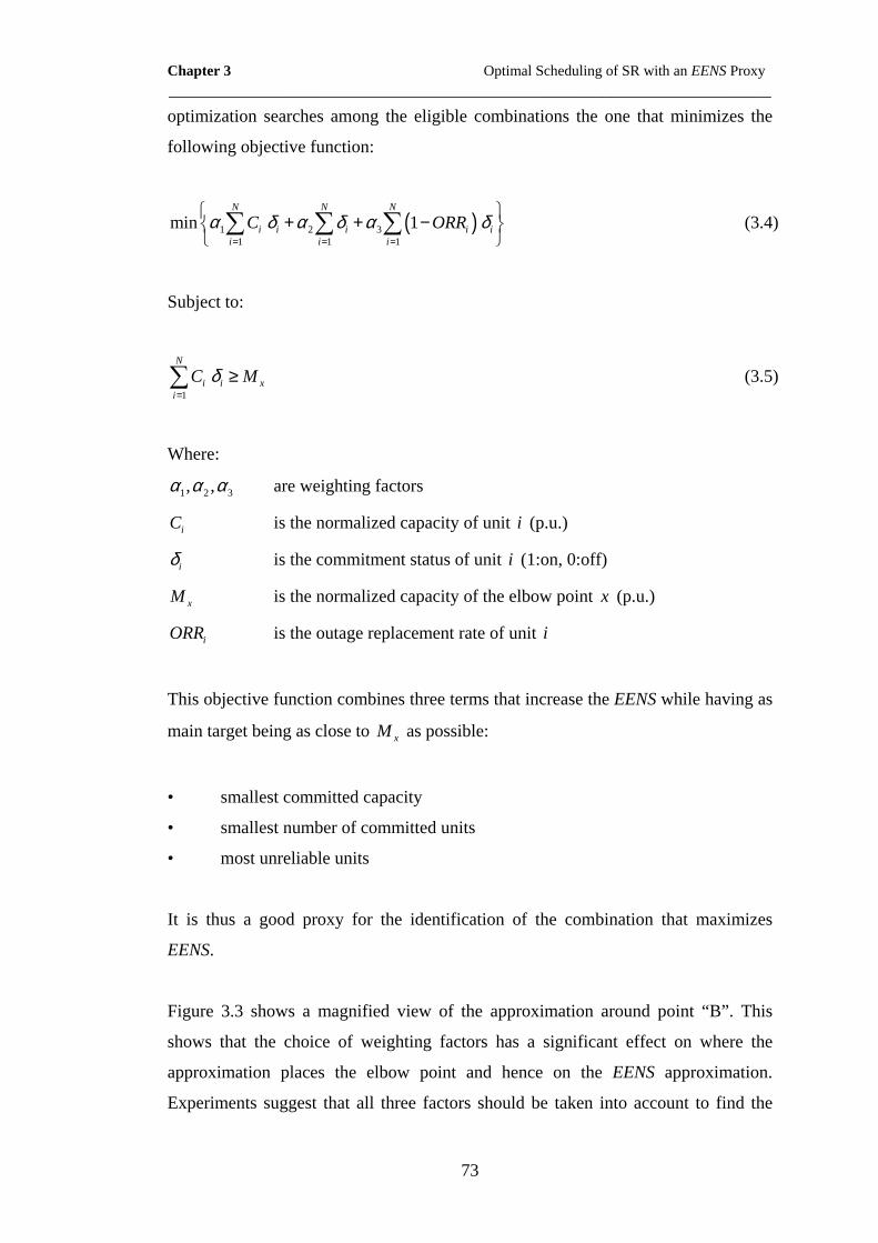
Chapter 3 Optimal Scheduling of SR with an EENS Proxy ____________________________________________________________________
73
optimization searches among the eligible combinations the one that minimizes the
following objective function:
( )1 2 31 1 1
min 1N N N
i i i i ii i i
C ORRα δ α δ α δ= = =
+ + − ∑ ∑ ∑ (3.4)
Subject to:
1
N
i i xi
C Mδ=
≥∑ (3.5)
Where:
1 2 3, ,α α α are weighting factors
iC is the normalized capacity of unit i (p.u.)
iδ is the commitment status of unit i (1:on, 0:off)
xM is the normalized capacity of the elbow point x (p.u.)
iORR is the outage replacement rate of unit i
This objective function combines three terms that increase the EENS while having as
main target being as close to xM as possible:
• smallest committed capacity
• smallest number of committed units
• most unreliable units
It is thus a good proxy for the identification of the combination that maximizes
EENS.
Figure 3.3 shows a magnified view of the approximation around point “B”. This
shows that the choice of weighting factors has a significant effect on where the
approximation places the elbow point and hence on the EENS approximation.
Experiments suggest that all three factors should be taken into account to find the
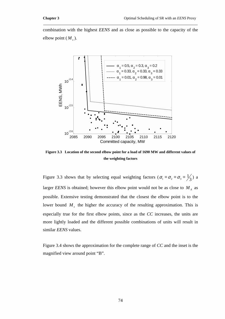
Chapter 3 Optimal Scheduling of SR with an EENS Proxy ____________________________________________________________________
74
combination with the highest EENS and as close as possible to the capacity of the
elbow point ( xM ).
2085 2090 2095 2100 2105 2110 2115 212010
-2.6
10-2.5
10-2.4
Committed capacity, MW
EE
NS
, MW
hα
1 = 0.5, α
2 = 0.3, α
3 = 0.2
α1 = 0.33, α
2 = 0.33, α
3 = 0.33
α1 = 0.01, α
2 = 0.98, α
3 = 0.01
Figure 3.3 Location of the second elbow point for a load of 1690 MW and different values of
the weighting factors
Figure 3.3 shows that by selecting equal weighting factors ( 1 2 31
3α α α= = = ) a
larger EENS is obtained; however this elbow point would not be as close to AM as
possible. Extensive testing demonstrated that the closest the elbow point is to the
lower bound xM the higher the accuracy of the resulting approximation. This is
especially true for the first elbow points, since as the CC increases, the units are
more lightly loaded and the different possible combinations of units will result in
similar EENS values.
Figure 3.4 shows the approximation for the complete range of CC and the inset is the
magnified view around point “B”.

Chapter 3 Optimal Scheduling of SR with an EENS Proxy ____________________________________________________________________
75
0 500 1000 1500 2000 2500 3000 350010-15
10-10
10-5
100
105
Committed Capacity, MW
EEN
S, M
Wh
2090 2100 2110 212010-2.6
10-2.3
α 1=0.50, α2=0.30, α3=0.20α 1=0.33, α2=0.33, α3=0.33α 1=0.01, α2=0.98, α3=0.01
A
C
B
Figure 3.4 Actual and approximated EENS as a function of the CC, L = 1690 MW. The inset shows a magnified view around point “B”
Thus, the objective of the auxiliary optimization process is firstly to be as close to
xM as possible (more weight should be given to the committed capacity, 1 0.5α = ),
and secondly, to select the largest EENS possible for such point. To achieve this,
more weight should be given to obtain an elbow point capacity with a lesser number
of units, 2 0.3α = . Considering the individual unreliability, 3 0.2α = is a reasonable
value because for a given committed capacity, the EENS is more sensitive to the
number of units committed, than to their individual unreliability. For systems with a
large number of relatively small generating units, 1α should be increased while 2α
and 3α should be decreased.
Once the combinations corresponding to each of the elbow points have been
identified, their exact EENS is computed using the COPT method. The number of
COPTs to be computed is thus equal to the number of steps in the piecewise
approximation plus 1. This auxiliary optimization procedure needs to be performed
once for the load level of each period in the scheduling horizon before the main UC
optimization. The application of the auxiliary optimization process is straightforward
and its computation prior to the main UC process averts the need to store hundreds
or thousands of EENS curves for every possible load level.

Chapter 3 Optimal Scheduling of SR with an EENS Proxy ____________________________________________________________________
76
3.5 ACCURACY OF THE APPROXIMATION
Figure 3.4 also compares the actual values of EENS and the values obtained using
this piecewise-linear approximation. The error is principally due the convexity of
each step of the EENS function (as illustrated by Figure 3.2). A feature of the
proposed approximation is that it does not underestimate the actual value; therefore
the UC optimization translates this overestimate into an excess of spinning reserve.
Such a systematic bias is desirable because it ensures consistency and errs on the
side of safety. This excess of reserve is the “price” paid for using an approximation
that makes the EENS calculation possible. Extensive testing demonstrated that the
approximation method based on the auxiliary optimization is more accurate and
consistent than other regression-based approximations.
Figure 3.5 shows that, as one would expect, the EENS increases with the load for a
given CC. It also shows that the shape of the EENS curve in the useful range remains
relatively unchanged as the elbow points shift to the right when the load increases.
1400 1600 1800 2000 2200 2400 2600 2800 3000 320010
-15
10-10
10-5
100
105
EE
NS,
MW
h
Committed capacity, MW
1500 MW 2000 MW 2500 MW
1750 MW 2250 MW 2750 MW
Figure 3.5 EENS approximation for various load levels in the IEEE-RTS
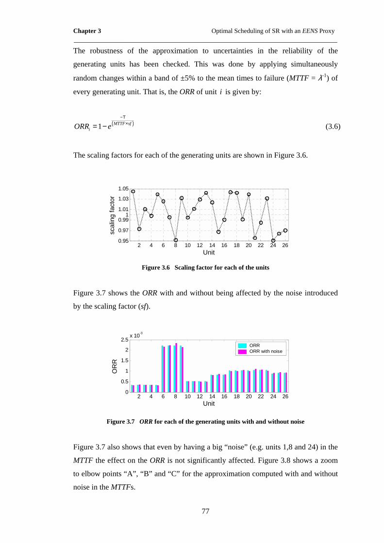
Chapter 3 Optimal Scheduling of SR with an EENS Proxy ____________________________________________________________________
77
The robustness of the approximation to uncertainties in the reliability of the
generating units has been checked. This was done by applying simultaneously
random changes within a band of ±5% to the mean times to failure (MTTF = λ-1) of
every generating unit. That is, the ORR of unit i is given by:
( )1 MTTF sfiORR e
−Τ×= − (3.6)
The scaling factors for each of the generating units are shown in Figure 3.6.
2 4 6 8 10 12 14 16 18 20 22 24 260.95
0.97
0.991
1.01
1.03
1.05
Unit
scal
ing
fact
or
Figure 3.6 Scaling factor for each of the units
Figure 3.7 shows the ORR with and without being affected by the noise introduced
by the scaling factor (sf).
2 4 6 8 10 12 14 16 18 20 22 24 260
0.5
1
1.5
2
2.5x 10⁻³
Unit
OR
R
ORRORR with noise
Figure 3.7 ORR for each of the generating units with and without noise
Figure 3.7 also shows that even by having a big “noise” (e.g. units 1,8 and 24) in the
MTTF the effect on the ORR is not significantly affected. Figure 3.8 shows a zoom
to elbow points “A”, “B” and “C” for the approximation computed with and without
noise in the MTTFs.

Chapter 3 Optimal Scheduling of SR with an EENS Proxy ____________________________________________________________________
78
1650 1700 1750100
101
Committed capacity, MWE
EN
S, M
Wh
2050 2100 215010-3
10-2
Committed capacity, MW
EE
NS
, MW
h
2450 2500 255010
-6
10-5
10-4
Committed capacity, MW
EE
NS
, MW
h
A B
C ORR
ORR with noise
Figure 3.8 Magnified views of elbow points “A”, “B” and “C” for approximations computed with and without noise in the MTTFs
These tests showed that the EENS approximation does not change significantly when
these random variations are applied. The auxiliary optimization process find the
same elbow points capacities, thus the differences between the two approximations
shown in Figure 3.8 are only in the EENS magnitude of the elbow point. However
these magnitudes are not significantly different as can be appreciated on the y-axis of
Figure 3.8.
3.6 IMPLEMENTATION OF THE PROPOSED UC
The proposed UC formulation has been implemented using Mixed Integer Linear
Programming in XpressMP (Dash Associates, 2005). Details of this formulation can
be found in Appendix C. With the exception of the minimum reserve requirement,
all the standard UC constraints are taken into account: power balance, upper and
lower generation limits, minimum up-times and minimum down-times, ramp-rate
limits, (Peterson and Brammer, 1995). The Mixed Integer Linear Programming
(MILP) formulation of the traditional UC is presented in Appendix C. The traditional
reserve constraint is replaced by an additional term in the objective function. Several

Chapter 3 Optimal Scheduling of SR with an EENS Proxy ____________________________________________________________________
79
auxiliary linear constraints are required to represent the piecewise linear
approximation of the EENS as a function of the CC.
The piecewise linear approximation is defined by the x- ( tX ) and y-coordinates ( tY )
of the “E” elbow points. That is, each elbow point is defined by its abscissa
( t teX ∈ X , MW) and its ordinate ( t t
eY ∈ Y , MWh) values. Since there are “E” elbow
points at each period of the optimization horizon, the cardinality of the coordinates
is: 1, ,e E= … .
For a given commitment of units at period t , the committed capacity ( tCC ) is
obtained using equation (3.3). Then, to relate tEENS to tCC , a decision variable tew
is associated with each elbow point of the approximation, (Williams, 1999, Guéret et
al., 2000):
1
Et t te e
eX w CC
=
=∑ (3.7)
1
Et t t
e ee
Y w EENS=
=∑ (3.8)
Only the variables tew corresponding to the endpoints of the appropriate segment
should be non-zero and their sum should be equal to one. Formally, this can be
expressed using the following equation:
11
Ete
ew
=
=∑ (3.9)
For each period, these three equations involve only three unknowns: tiw , t
jw and
tEENS . On the other hand, tCC is known. The tew decision variables are found
through the optimization process and hence the value of tEENS .

Chapter 3 Optimal Scheduling of SR with an EENS Proxy ____________________________________________________________________
80
For instance, suppose that a period t the load to serve is 1690 MW, and the units are
committed and dispatched as shown in Figure 3.9.
2 4 6 8 10 12 14 16 18 20 22 24 260
100
200
300
400
Unit
MW
Power producedActual capacity
Figure 3.9 Commitment and dispatch, L = 1690 MW
For the commitment and dispatch shown in Figure 3.9 the committed capacity is
2105 MW. The computed EENS using the COPT is 0.0029064 MWh. Applying the
auxiliary optimization process proposed, the coordinates of the elbow points are as
shown in Table 3.1.
Table 3.1 Elbow points, L = 1690 MW
e teX , (MW) t
eY , (MWh)
1 12 1678
2 1691 1.5477
3 2090 0.0030794
4 2490 2.7069×10⁻⁶
5 2841 1.3184×10⁻⁹
6 3105 1.5249×10⁻¹²
Table 3.1 shows that the tCC = 2105 MW lies between elbow points 3 and 4. Thus,
applying equations (3.7) to (3.9) the following linear system is obtained:
36
4
2090 2490 0 21050.0030794 2.7069 10 1 0
1 1 0 1
t
t
t
ww
EENS
−
× − =
(3.10)

Chapter 3 Optimal Scheduling of SR with an EENS Proxy ____________________________________________________________________
81
The solution of this system of equations is:
3
4
0.96250.0375
0.002964
t
t
t
ww
EENS
=
(3.11)
It can be appreciated that the EENS obtained with the piecewise approximation
(equation (3.11)) is very close to the actual value obtained building the COPT, but
slightly higher. It should also be noted that, with mathematical rigor, the tCC of the
proposed scheduling is contained in more than one pair of elbow points; for instance
between coordinates: (1,4), (2,4), (3,5), etc. However, other combinations rather
than (3,4) result in a larger EENS; and since the EENS is penalized in the objective
function, the pair that results in the smaller EENS is selected in the optimization
process. Figure 3.10 show different possible lines joining adjacent and nonadjacent
elbow points. Note that point 1 is not considered since it involves load curtailments.
For the cases in which the line joins nonadjacent elbow points the resulting EENS is
significantly larger.
1800 2000 2200 2400 2600 2800
10-8
10-6
10-4
10-2
100
Committed capacity, MW
EE
NS
, MW
h
(2,3)
(3,4)
(4,5)
(2,4)
(3,5)
(2,5) 2
3
4
5
Figure 3.10 Approximation of the EENS as a function of the CC for different elbow points, L = 1690 MW

Chapter 3 Optimal Scheduling of SR with an EENS Proxy ____________________________________________________________________
82
Formally, further constraints can be enforced in order to guarantee that the non-zero tew variables correspond to adjacent elbow points:
11
2
1
tt
t
tEt
E
wb
w
bw −
≤
M ""
(3.12)
1
11
Ets
sb
−
=
=∑ (3.13)
Where:
M is an ( )1E E× − matrix such that:
1ijm = i j∀ = and 1i j= +
0ijm = otherwise
tsb is a binary variable ( [ ]0,1t
sb ∈ ) such that:
1tsb = if tCC lays within segment “ s ”
0tsb = otherwise.
For the example presented, equation (3.12) results in:
11
22
33
44
55
6
1 0 0 0 01 1 0 0 00 1 1 0 00 0 1 1 00 0 0 1 10 0 0 0 1
tt
tt
tt
tt
tt
t
wb
wb
wb
wb
wb
w
≤
(3.14)
And since only one variable “ tsb ” can be 1, thus it is not possible to select
nonadjacent tew s. Therefore, with 3 1tb = , then: 3 0tw ≥ and 4 0tw ≥ , but satisfying that
4 3 1t tw w+ = . However it should be noted that by enforcing constraints (3.12) and

Chapter 3 Optimal Scheduling of SR with an EENS Proxy ____________________________________________________________________
83
(3.13), an extra binary variable is required and this results into unnecessary
computational burden. However, they are presented for the sake of mathematical
formality, since as it has been mentioned, nonadjacent elbow points are never
selected because of their higher EENS associated.
3.7 TEST RESULTS
The proposed UC formulation was tested on two systems. The results are shown
separately.
3.7.1 Results on the IEEE-RTS Single-Area System
The first system is the IEEE-RTS one area system without hydro generation. This
system consists of 26 units, for which the UC data and ramp rate limits were
obtained from (Wang and Shahidehpour, 1993), and the start-up costs and reliability
data from (Grigg et al., 1999). Details can be found in Appendix B. The power
generated by the units committed at 0t = is given by the economic dispatch of the
committed units for the first period for a load level of 1700 MW. Perfect competition
is assumed in the test simulations among the generating units; i.e. the market surplus
is maximized. Optimizations were performed using a branch and bound technique in
XpressMP, (Dash and Associates, 2005), and a MIP gap no larger than 0.075% was
considered adequate. The load profile used for testing was taken from (Wang and
Shahidehpour, 1993), and is shown in Figure 3.11.

Chapter 3 Optimal Scheduling of SR with an EENS Proxy ____________________________________________________________________
84
0 4 8 12 16 20 241600
1800
2000
2200
2400
2600
2800
time period, hrs
p d, MW
Figure 3.11 Load profile used for testing
Figure 3.12.a shows the schedule computed by the UC implementing the
conventional reserve constraint with a reserve requirement equal to the capacity of
the largest committed generating unit. And Figure 3.12.b shows the schedule
obtained with a UC program implementing the proposed formulation, considering a
VOLL of 1,500 $/MWh.
4 8 12 16 20 24
5
10
15
20
25
time period, hrs
unit
4 8 12 16 20 24
5
10
15
20
25
time period, hrs
unit
a) Traditional UC formulation for: ( )maxmaxt t
d i ir u P= b) Proposed UC formulation for
VOLL = 1,500 $/MWh
Figure 3.12 Schedules obtained with different formulations

Chapter 3 Optimal Scheduling of SR with an EENS Proxy ____________________________________________________________________
85
Figure 3.12 show that the resulting schedules are different. Enforcing the traditional
constraint for the reserve requirements results in more units being scheduled in order
to maintain the specified amount tdr . Since the proposed approach does not schedule
as many units, at some periods, it provides less SR. For instance, at period 11, with
the traditional approach all units except unit 9 are committed, while the proposed
approach shows that it is cheaper to take a risk and not commit as much expensive
generation as the traditional reserve constraint requires.
Figure 3.13 compares the amount of SR scheduled by the two methods. The
traditional method schedules at every hour at least 400 MW of reserve because that
is the capacity of the largest scheduled unit. For the chosen VOLL, the proposed
approach schedules a smaller amount of reserve because it determines that the cost
of providing this reserve is not justified in terms of a reduction in EENS. Because of
the ramp rate constraints, the traditional formulation minimizes the operating cost by
dispatching the generating units in such a way that the reserve provided is exactly
equal to the deterministic requirement at all periods. On the other hand, the proposed
formulation takes into account the changes in the load level and the combinations of
units at each period. This results in different estimates of EENS at each period.
Furthermore, the proposed approach determines how much reserve this EENS
justifies, taking into consideration the cost of providing it.
0 4 8 12 16 20 24300
350
400
450
500
time period, hrs
Res
erve
, MW
SR, TraditionalSR, Proposed
Figure 3.13 Comparison of the spinning reserve scheduled by the traditional UC and the proposed formulation
Figure 3.14 illustrates the influence that VOLL has on the results. To make the
results more generally applicable, all costs have been normalized using as a basis the
sum of the running and start-up costs for the traditional UC and the standard rule-of-

Chapter 3 Optimal Scheduling of SR with an EENS Proxy ____________________________________________________________________
86
thumb for the reserve requirement (in this case ( )maxmaxt td i ir u P= ). Similarly, VOLL
has been normalized on the basis of the average cost of electrical energy for the same
UC case (13.493 $/MWh). The x-scale is logarithmic in order to highlight the
differences between the two formulations for low VOLLs. In this and subsequent
figures, the EENS cost has been calculated using the technique described in
(Billinton and Allan, 1996) not the approximation used for the optimization.
102 1035.7
5.8
5.9
6
6.1
x 10-3
VOLL, p.u.
star
t-up
cost
, p.u
.
102 1030.99
0.992
0.994
VOLL, p.u.
prod
uctio
n co
st, p
.u.
102 1030
0.005
0.01
0.015
VOLL, p.u.
EE
NS
cos
t, p.
u.
102 1030.98
0.99
1
1.01
1.02
VOLL, p.u.
tota
l cos
t, p.
u.
TraditionalProposed
TraditionalProposed
TraditionalProposed
TraditionalProposed
103.1 103.4
1.0031.005
Figure 3.14 Normalized costs as a function of the normalized VOLL. The inset in the lower right figure shows a magnification on a VOLL range of 17,000 and 34,000 $/MWh
As one would expect, Figure 3.14 shows that, for the traditional UC formulation, the
start-up and production costs are independent of VOLL while the EENS cost
increases with VOLL. On the other hand, with the proposed formulation, the different
costs change with VOLL to achieve a minimum total cost. Over most of the range of
VOLL, the proposed approach produces a solution with a total cost lower than the
one obtained with the traditional UC. For a small range of VOLL (around 25,000
$/MWh), the traditional method is slightly cheaper because the approximation in the
calculation of the EENS causes a slight overestimation of this cost and because the
deterministic reserve criterion happens to deliver the optimal amount of reserve for
this specific VOLL.

Chapter 3 Optimal Scheduling of SR with an EENS Proxy ____________________________________________________________________
87
Figure 3.15 shows the effect of reducing the deterministic reserve requirement in the
traditional UC formulation to 380tdr = MW and increasing it to 420t
dr = MW.
When the requirement is reduced, the EENS cost for the traditional approach
increases significantly. While the operating cost decreases, the total cost increases.
Conversely, when this requirement is increased, the EENS cost decreases, but the
operating cost and the total cost increase. In all cases the difference in total cost
between the deterministic and probabilistic approaches are significant. As shown, the
choice of deterministic criterion would have significant consequences on the overall
cost of the scheduling, producing suboptimal solutions for almost all VOLLs.
102
103
0
0.005
0.01
0.015
VOLL, p.u.
EE
NS
cos
t, p.
u. TraditionalProposed
102
103
0.98
0.99
1
1.01
1.02
VOLL, p.u.
tota
l cos
t, p.
u.
TraditionalProposed
102
103
0
0.005
0.01
0.015
VOLL, p.u.
EE
NS
cos
t, p.
u. TraditionalProposed
102
103
0.98
0.99
1
1.01
1.02
VOLL, p.u.
tota
l cos
t, p.
u.
TraditionalProposed
rd = 380 MW
rd = 380 MW
rd = 420 MW
rd = 420 MW
Figure 3.15 EENS costs and total costs for different deterministic criteria
If the system operator is reluctant to set the spinning reserve using a probabilistic
technique, the traditional reserve constraint can be included in the problem
formulation at the same time as the EENS cost is included in the objective function.
The amount of reserve scheduled in this hybrid formulation is therefore never less
than that specified by the deterministic criterion. On the other hand, when VOLL is
large and the risk of load shedding is significant, this hybrid approach provides more
reserve. Figure 3.16 contrasts the reserve provided by the hybrid and traditional
formulations when VOLL is 20,000 $/MWh. During some periods the hybrid
formulation schedules slightly more reserve than the traditional formulation. For the

Chapter 3 Optimal Scheduling of SR with an EENS Proxy ____________________________________________________________________
88
remaining periods, the reserve scheduled by both formulations is the same. In both of
these cases the committed capacity is at or beyond the second elbow point of the
EENS approximation.
0 4 8 12 16 20 24390
395
400
405
410
time period, hrs
Res
erve
, MW
SR, TraditionalSR, Proposed
Figure 3.16 Spinning reserve scheduled by the traditional and the hybrid UC formulations
By scheduling the units in a different way, and providing a small extra amount of
SR, the hybrid formulation attains savings in the overall operation of the system, as
shown in Figure 3.17. This figure also shows that the main savings are attained by
means of starting up fewer units, and dispatching them differently. This generates an
increase in the dispatch cost, but also a reduction in the EENS cost, the overall total
is lower than the traditional approach.
1 2 3 4-100
-50
0
50
100
savi
ngs,
$
cost component, $
1.- start-up2.- dispatch3.- EENS 4.- total
Figure 3.17 Itemized savings for the hybrid UC formulation compared with the traditional formulation
It must also be noted that this hybrid approach can be used to estimate the marginal
cost of imposing deterministic criteria on the SR procurement. Since, for some
periods the deterministic criterion hinders the optimization process ability to attain
the overall economical benefit derived from trading the SR cost versus its benefit.

Chapter 3 Optimal Scheduling of SR with an EENS Proxy ____________________________________________________________________
89
3.7.2 Results on the IEEE-RTS Three-Area System
The IEEE-RTS96 three areas system without hydro generation has also been used to
test the proposed UC formulation. This system consists of 78 units in which the UC
data for a single area and ramp rate limits were taken from (Wang and Shahidehpour,
1993), the cost functions of the remaining areas are scaled by a factor of 1.03 and
1.06 respectively in order to obtain different marginal prices for the production of
electrical energy of each generating unit. The units were sorted in ascending
capacity. The reliability data was taken from (Grigg et al., 1999). The power
generated by the units committed at 0t = was assumed to be given by the economic
dispatch of the committed units for the first period for a load level of 5100 MW.
Optimizations were performed using a branch and bound technique in XpressMP
(Dash Associates, 2005), and a MIP gap no larger than 0.075% was considered
adequate. Figure 3.18 shows the load profile used for testing.
0 4 8 12 16 20 244500
5000
5500
6000
6500
7000
7500
8000
8500
time period, hrs
p d, MW
Figure 3.18 Load profile used for testing in the IEEE-RTS three-area system
Figure 3.19.a shows the schedule obtained by using the conventional reserve
constraint with a reserve requirement equal to the capacity of the largest committed
generating unit; and Figure 3.19.b shows the schedule obtained applying the
proposed UC approach for a VOLL of 1,500 $/MWh.

Chapter 3 Optimal Scheduling of SR with an EENS Proxy ____________________________________________________________________
90
6 12 18 24 30 36 42 48 54 60 66 72 78
4
8
12
16
20
24
unit
time
perio
d, h
rs
a) Schedule using the traditional reserve constraint, ( )maxmaxt t
d i ir u P=
6 12 18 24 30 36 42 48 54 60 66 72 78
4
8
12
16
20
24
unit
time
perio
d, h
rs
b) Schedule using the proposed UC formulation, VOLL = 1,500 $/MWh
Figure 3.19 Schedules obtained using different UC approaches in the IEEE-RTS three-area system
By comparing Figure 3.19.a with Figure 3.19.b it can be appreciated that each UC
approach commits the units in a different way. While the traditional UC approach
commits more small generation in the middle of the optimization horizon, the
proposed approach commits unit 36 from the very beginning of the schedule. Figure
3.20 compares the amount of SR provided by the two methods. The traditional
method provides at every hour at least 400 MW of reserve because that is the
capacity of the largest scheduled unit. For the chosen VOLL, the proposed approach
schedules the same amount of SR and at the early periods a slightly higher amount
than the deterministic criterion. This is because unit 36 is committed from the very
beginning and the units are dispatched in the most economical way, but spare
capacity is still committed. On the other hand, from period 8 by committing unit 36
the commitment of unit 10 is averted, and the overall scheduling is less costly than
using the traditional rule of thumb.

Chapter 3 Optimal Scheduling of SR with an EENS Proxy ____________________________________________________________________
91
0 4 8 12 16 20 24300
400
500
600
700
800
900
1000
1100
time period, hrs
Res
erve
, MW
SR, TraditionalSR, Proposed
Figure 3.20 Comparison of the spinning reserve scheduled by the traditional UC and the proposed formulation for VOLL = 1,500 $/MWh
For VOLLs between 500 $/MWh and 25,000 $/MWh in this system, it is not
justifiable to schedule less SR than the traditional rule of thumb. On the other hand,
for higher VOLLs the proposed UC formulation sets larger amounts of SR compared
to the UC enforcing the traditional SR requirement. Figure 3.21 contrasts the SR
scheduled by the traditional formulation and the proposed formulation for a VOLL of
32,000 $/MWh
0 4 8 12 16 20 24200
300
400
500
600
700
800
900
1000
1100
1200
time period, hrs
Res
erve
, MW
SR, TraditionalSR, Proposed
Figure 3.21 SR scheduled by both approaches for VOLL = 32,000 $/MWh

Chapter 3 Optimal Scheduling of SR with an EENS Proxy ____________________________________________________________________
92
Figure 3.22 illustrates the influence that VOLL has on the results. To make the
results more generally applicable, all costs have been normalized using as a basis the
sum of the running and start-up costs for the traditional UC and the standard rule-of-
thumb for the reserve requirement (in this case 400tdr = MW). Similarly, VOLL has
been normalized on the basis of the average cost of electrical energy for the same
UC case (13.186 $/MWh), the x-scale is logarithmic in order to highlight the
differences between the two formulations for low VOLLs.
102
103
3
4
5
6
7x 10
-3
VOLL, p.u.
star
t-up
cost
, p.u
.
TraditionalProposed
102
103
0.99
0.992
0.994
0.996
0.998
1
VOLL, p.u.
prod
uctio
n co
st, p
.u.
TraditionalProposed
102
103
0
0.005
0.01
0.015
VOLL, p.u.
EE
NS
cos
t, p.
u. TraditionalProposed
102
103
0.98
0.99
1
1.01
1.02
VOLL, p.u.
tota
l cos
t, p.
u.
TraditionalProposed
Figure 3.22 Normalized costs as a function of the normalized VOLL
As for the single area test system, Figure 3.22 shows that, for the traditional UC
formulation, the start-up and production costs are independent of VOLL while the
EENS cost increases with VOLL. On the other hand, with the proposed formulation,
the different costs change with VOLL to achieve a minimum total cost. Over all the
range of VOLL, the proposed approach produces a solution with a total cost lower
than the one obtained with the traditional UC.
Figure 3.22 also shows that the EENS cost presents an abrupt drop around 25,000
$/MWh. This is because beyond this point the increase in the EENS cost compels the
system to schedule larger amounts of SR. Clearly, this extra spare capacity in the

Chapter 3 Optimal Scheduling of SR with an EENS Proxy ____________________________________________________________________
93
system reduces the EENS cost but at the same time increases the production cost;
that is the reason why the production costs exhibits an abrupt increase for the same
VOLL. However, the overall cost of the commitment remains below the cost
obtained with the traditional UC formulation.
Figure 3.23 shows the effect of reducing the deterministic reserve requirement in the
traditional UC formulation to 380tdr = MW and increasing it to 420t
dr = MW at all
periods of the optimization horizon. When the requirement is reduced, the EENS cost
for the traditional approach increases significantly. While the operating cost
decreases, the total cost increases. Conversely, when this requirement is increased,
the EENS cost decreases, but the operating cost and the total cost increase. However,
when the deterministic criterion is increased, for VOLLs beyond 25,000 $/MWh the
overall difference between the traditional and the proposed UC formulation
decreases. This points to the conclusion that the system requires a larger amount of
SR. In essence, this is because there are more generating units in the system and
hence more chances of suffering multiple outages.
102 1030
0.005
0.01
0.015
VOLL, p.u.
EE
NS
cos
t, p.
u. TraditionalProposed
102 1030.98
0.99
1
1.01
1.02
VOLL, p.u.
tota
l cos
t, p.
u.
TraditionalProposed
102 1030
0.005
0.01
0.015
VOLL, p.u.
EE
NS
cos
t, p.
u. TraditionalProposed
102 1030.98
0.99
1
1.01
1.02
VOLL, p.u.
tota
l cos
t, p.
u.
TraditionalProposed
rd = 380 MW
rd = 380 MW
rd = 420 MW
rd = 420 MW
VOLL = 25,000 $/MWh
Figure 3.23 EENS costs and total costs for different deterministic criteria

Chapter 3 Optimal Scheduling of SR with an EENS Proxy ____________________________________________________________________
94
3.8 CONCLUSIONS
This chapter presents a novel UC formulation that takes into account directly the cost
of unreliability. This cost is included in the objective function as the product of the
Expected Energy Not Served and the Value of Lost Load. Instead of imposing a
deterministic spinning reserve requirement, the proposed method considers the
probability of generation outages that might require load shedding and the cost of
providing enough reserve to preclude the need for such load shedding. Compared
with the traditional approach for the provision of spinning reserve, the proposed
approach strikes a better balance between the cost and the benefit of providing
reserve; therefore it can produce significant savings in the total cost of operating the
power system, including the socio-economic cost of outages.
The key to the implementation of this approach is the development of an efficient
method for calculating an approximate value of the EENS that would result from the
commitment of a particular combination of generating units. Even though this
approximation tends to overestimate the value of EENS and thus results in an over-
commitment of reserve, in most cases the proposed method results in a lower cost
than the traditional UC formulation.
Compared with (Gooi et al., 1999, Chattopadhyay and Baldick, 2002), this approach
does not require external cost/benefit analyses for the selection of the risk level to be
attained, since these trade-offs are performed at each period of the optimization
horizon within the scheduling calculation.
The traditional reserve constraint can also be combined with the proposed
formulation. This hybrid method guarantees that at least the amount of reserve
specified by the deterministic criteria will be scheduled at all time. For periods when
the probability of load shedding is high, it will schedule a larger amount of reserve to
reduce the expected cost of not supplying consumers.
The proposed formulation is self-contained and does not require external calculations
of the benefits to consumers of the provision of a certain amount of reserve. The
schedule is obtained in a single UC run and has a lower cost than what can be

Chapter 3 Optimal Scheduling of SR with an EENS Proxy ____________________________________________________________________
95
achieved using a traditional UC formulation with different deterministic reserve
criteria. Furthermore, by being self-contained, this approach does not require setting
a risk level to attain, and thus problems of suboptimal solutions and infeasibility are
averted.

Chapter 4 Optimal Scheduling of SR Considering FS with EENS proxies ____________________________________________________________________
96
Chapter 4
Optimal Scheduling of Spinning Reserve
Considering the Failure To Synchronize with
EENS Proxies
4.1 INTRODUCTION
The probabilistic scheduling of spinning reserve described in the previous chapter
considers only the probability that the generating units undergo to outage state from
a fully available state; and it neglects the probability of the units of failing to
synchronize (FS) successfully with the power system. In the open literature can be
found reports describing this failure to synchronize of peaking and cycling units as a
common event. A more comprehensive assessment of the EENS should include a
reliability model of the generating units that takes into account the failures to
synchronize.
This chapter deals with the analytical development and Monte Carlo validation of a
three-state generating unit model that explicitly considers the probability of failing to
synchronize of the units starting-up. This model is used to compute a more accurate
value of the EENS for a given combination of units. It also proposes a set of linear
constraints to include the three-state model in the unit commitment (UC)
optimization process. By including this model, a better balance between the societal
cost of the expected unserved electrical energy and the cost of providing the spinning
reserve (SR) is attained.

Chapter 4 Optimal Scheduling of SR Considering FS with EENS proxies ____________________________________________________________________
97
4.2 GENERATING UNIT MODELS
In order to develop generating units models suitable for planning or for operating
studies in power systems it is required to have actual data of the units� performance.
In particular, for unit commitment studies, this data is concerned with the unit�s
availability. In North America this data is compiled by two national organizations.
In the United States utility data are processed and disseminated by the North
American Reliability Council, (NERC, 2006), through the Generating Availability
Data Systems, (GADS, 2005). In Canada, the Canadian Electrical Association
(CEA, 2004) handles these data through its Equipment Reliability Information
System (ERIS), (CEA, 1995). The databases of both systems contain a considerable
amount of raw data, which can be interrogated to produce additional statistics and
models for performance evaluation and system reliability assessment.
4.2.1 Unit Operating States
It is a standard practice for most of the electric utilities around the world to collect
data on the operating history of their generating units. Details of the data collection
procedure may vary from one utility to another but the basic intent remains the same.
In Canada, for instance, all the possible generating unit states are classified into
eleven groups or states as shown in Table 4.1, (Debnath and Billinton, 1989).
Table 4.1 Unit States
No. Name of the state
Available states
1 Operating � Full capacity
2 Operating � Forced derating
3 Operating � Scheduled derating
4 Available but not operating � Full capacity
5 Available but not operating � Forced derating
6 Available but not operating � Scheduled derating
Non-available states
7 Forced outage

Chapter 4 Optimal Scheduling of SR Considering FS with EENS proxies ____________________________________________________________________
98
8 Forced extension of maintenance outage
9 Forced extension of planned outage
10 Maintenance outage
11 Planned outage
This eleven-state model is the most complete. By continuous state monitoring and
conventional statistics the transition rates associated with each the unit states can be
obtained. The basic data can also be used to generate multi-state models suitable for
specific studies (e.g. operation or planning).
The traditional model used in reliability studies consists of two states. Either the
generating unit is fully operative or fully inoperative. However this model does not
represent the probability of the unit failing to synchronize with the power system.
For cycling or peaking units it is especially important to represent the state transition
between an available but not operating state to either an operating state or a forced
outage state. Peak load units or cycling units are intended for operation during peak
loads, which are short in duration. Therefore these units spend more time in the
available but not operating states than in the operating states. On the other hand,
base load units are intended for operation whenever they are available. These units
should therefore spend most of their available time in the operating states with little
or no time in the available but not operating states. This is shown in Figure 4.1,
which shows the states probabilities estimated for the state residence times of nuclear
units with capacities ranging from 400 MW to 599 MW and Combustion Turbine
Engines (CTU) ranging from 25 MW to 49 MW, (Debnath and Billinton, 1989).
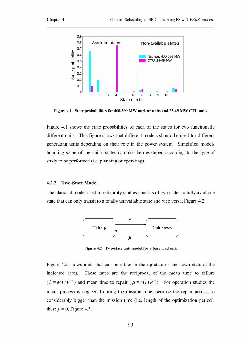
Chapter 4 Optimal Scheduling of SR Considering FS with EENS proxies ____________________________________________________________________
99
1 2 3 4 5 6 7 8 9 10 110
0.1
0.2
0.3
0.4
0.5
0.6
0.7
0.8
0.9
State number
Sta
te p
roba
bilit
y
Nuclear, 400-599 MWCTU, 24-49 MW
Availabe states Non-availabe states
Figure 4.1 State probabilities for 400-599 MW nuclear units and 25-49 MW CTU units
Figure 4.1 shows the state probabilities of each of the states for two functionally
different units. This figure shows that different models should be used for different
generating units depending on their role in the power system. Simplified models
bundling some of the unit�s states can also be developed according to the type of
study to be performed (i.e. planning or operating).
4.2.2 Two-State Model
The classical model used in reliability studies consists of two states, a fully available
state that can only transit to a totally unavailable state and vice versa, Figure 4.2.
Unit up Unit down
λ
µ
Unit up Unit down
λ
µ
Figure 4.2 Two-state unit model for a base load unit
Figure 4.2 shows units that can be either in the up state or the down state at the
indicated rates. These rates are the reciprocal of the mean time to failure
( 1MTTFλ −= ) and mean time to repair ( 1MTTRµ −= ). For operation studies the
repair process is neglected during the mission time, because the repair process is
considerably bigger than the mission time (i.e. length of the optimization period);
thus: µ = 0, Figure 4.3.

Chapter 4 Optimal Scheduling of SR Considering FS with EENS proxies ____________________________________________________________________
100
Unit up Unit downλ
Unit up Unit downλ
Figure 4.3 Two-state mission oriented model
This is a Markovian1 process, and its dynamic equation is given by:
( )( )upup
d P tP t
dtλ= − (4.1)
Solving this differential equation, we get:
( ) tupP t e λ−= (4.2)
And since ( ) ( ) 1up downP t P t+ = , the probability of being in the down state is given by:
( ) 1 tdownP t e λ−= − (4.3)
The last equation represents the probability that a unit goes on outage at any time
during the mission time and is not repaired. This probability is also known as the
Outage Replacement Rate (ORR), (Billinton and Allan, 1996).
4.2.3 Four-State Model
Difficulties can be encountered in applying the two-state model to units that operate
during peak periods or cycling units, since these units spend most of the time in
�available but not operating� state. In other words, the periods of service are
interrupted by periods of scheduled shutdown in order to minimize the overall
operating cost. The frequent start-ups and shutdowns subject the unit to additional
starting stress compared to base load units. This additional starting stress has been
1 Stochastic process in which the conditional probability distribution of future states, given the present state, depends only upon the current state, i.e. it is conditionally independent of the past states (the path of the process) given the present state.

Chapter 4 Optimal Scheduling of SR Considering FS with EENS proxies ____________________________________________________________________
101
recognized and reported as failure-to-start or starting failure outage, (GADS, 2005,
CEA, 1995). More complete models that take into consideration these aspects have
been developed and reported. The most widely accepted unit model that takes this
stress into account is the four-state model developed by the IEEE task group on
models for peaking service units (Calsetta et al., 1972). This model is shown in
Figure 4.4.
Reserve shutdown In service
(1-Ps)/T
1/D
Forced outbut not needed
Forced out inperiod of need
1/T
1/D
λµ Ps/T µ
0 2
1 3
Reserve shutdown In service
(1-Ps)/T
1/D
Forced outbut not needed
Forced out inperiod of need
1/T
1/D
λµ Ps/T µ
0 2
1 3
Figure 4.4 Four state model for planning studies
Where in this model T represents the average reserve shut down time between
periods of need, exclusive of periods for maintenance or other planned unavailability
(hrs.), D is the average in-service time per occasion of demand (hrs.) and Ps is the
probability of a starting failure resulting in inability to serve load during all or part of
a demand period. Repeated attempts to start during one demand period should not
be interpreted as more than one failure to start.
The parameters λ, µ and Ps can be estimated from the unit operating data. The D
and the T however depend on the role that the generating unit has in the power
system.
This four state model is also a Markovian process, and its equation is as follows:

Chapter 4 Optimal Scheduling of SR Considering FS with EENS proxies ____________________________________________________________________
102
( )( )( )( )
( )( )( )( )
0 0
1 1
2 2
3 3
1 1 0
1 10 0
1 10
1 1
T DP t P t
T DP t P tdPsP t P tdt
T DP t P tPsT T D
µ
µ
λ µ
λ µ
−
− + = − − +
− +
(4.4)
Again, for operation studies the repair process is neglected since it is larger than the
mission time. The average in-serve time per occasion of demand (D) is also greater
than the mission time; therefore the model is reduced to the one shown in Figure 4.5.
Reserve shutdown In service
(1-Ps)/T
Forced outbut not needed
Forced out inperiod of need
1/T
λPs/T
0 2
1 3
.
Reserve shutdown In service
(1-Ps)/T
Forced outbut not needed
Forced out inperiod of need
1/T
λPs/T
0 2
1 3
.
Figure 4.5 Four-state mission oriented model
Figure 4.5 shows that state 1 cannot be reached. Since this model will be used for
cyclic and peaking units it will always depart from state 0. A unit can transit to either
forced outage in period of need or to a successful synchronization (in service). In the
case of a successful synchronization, the unit can still fail and thus undergo a forced
outage. The time dependent probability of each of the states can be found by means
of solving the model�s equation, (equation (4.5)).
Chapter 4 Optimal Scheduling of SR Considering FS with EENS proxies ____________________________________________________________________
103
( )( )( )( )
( )( )( )( )
0 0
1 1
2 2
3 3
1 0 0 0
10 0 0
1 0 0
1 0
TP t P tP t P td TP t P tPsdt
TP t P tPsT T
λ
λ
− − = − −
(4.5)
Alternatively equation (4.5) can be rewritten using matrix notation:
( ) ( )t t•
=P Λ P (4.6)
Applying the Laplace transform to equation (4.6) it is obtained:
( ) ( ) ( )0s s s− =P P Λ P (4.7)
It is known that the generating unit was operating in reserve shutdown state at t = 0,
therefore the vector of initial conditions is: ( ) [ ]0 1 0 0 0 T=P . Equation (4.7)
can be rewritten as:
( ) ( ) ( )1 0s s −= −P I Λ P (4.8)
Doing the algebraic steps required by equation (4.8), one gets:
( )( )( )
( )( )
10
11
1
TsT
Psss sT
s Pss sT s
λλ
λ
+ −=
+ + +
+ +
P (4.9)
Applying the inverse Laplace transform to equation (4.9) gives:
Chapter 4 Optimal Scheduling of SR Considering FS with EENS proxies ____________________________________________________________________
104
( )0
11
111 1
tT
tt T
ttT
e
Pst e eT
T Ps Pse eT T
λ
λ
λ
λλ λ
−
−−
− −
−= − − − − + + − −
P (4.10)
The IEEE four-state model is used for planning studies; therefore some
considerations have to be made to consider a more accurate model for operation
studies:
• As mentioned earlier, the repair process is larger than the mission time, thus,
it is neglected
• Each of the optimization periods is considered independent
• During each period of the optimization horizon, the units that are being
synchronized will not be shut down, thus: T→0. That is, the unit can fail to
synchronize and can also fail during its mission time, but it will not be shut
down during optimization period in which it has been committed
When T→0 the model is reduced, and P2(t) represents the availability of the model
and P3(t) the unavailability of the model:
( ) ( )2t tA t P t e Ps eλ λ− −= = − (4.11)
( ) ( )3 1 t tU t P t e Ps eλ λ− −= = − + (4.12)
From equations (4.11) and (4.12) it can be seen that the equality A(t) + U(t) = 1
holds. These equations also show that if the units never fail to synchronize (i.e. Ps =
0), then U(t) reduces to the traditional ORR, and A(t) to 1 � ORR. The unavailability
denoted by equation (4.12) is named probability of failure in the remaining of this
Chapter (Pf).

Chapter 4 Optimal Scheduling of SR Considering FS with EENS proxies ____________________________________________________________________
105
The parameter Ps (probability of a starting failure) is estimated form historical data
as follows:
total start failurestotal attempted starts
Ps = (4.13)
The Pf can also be obtained in an intuitive way as follows: The probability of a unit
residing the available state is obtained by the product of the probability of successful
synchronization and the probability that it will not fail during the mission time:
( ) ( )( )1 1A t Ps ORR= − − (4.14)
Therefore the unavailability or probability of failure (Pf) of the generating unit is
given as:
( )( )1 1 1Pf Ps ORR= − − − (4.15)
Since the failures are exponentially distributed then, 1 tORR e λ−= − . The result of
replacing the ORR in equation (4.15) is consistent with equation (4.12).
Summarizing, for the units that have been synchronized in the previous period of the
commitment, the probability of failure in the current period will be given directly by
its ORR. On the other hand, if the unit is being synchronized, then the probability
that it fails in the current period of the commitment will be given by equation (4.15).
4.3 EENS CALCULATION
For the EENS calculation the two models presented in the previous section are
required to generate the COPT, (refer to appendix A for details) and then to compute
the EENS as explained in (Billinton and Allan, 1996). For a given combination of
units, we must know which of them are being started up and which have been
synchronized in the previous period in order to use the adequate unit model.
Chapter 4 Optimal Scheduling of SR Considering FS with EENS proxies ____________________________________________________________________
106
Once the COPT is computed, the EENS will be sensitive to the following factors:
• The load level to supply
• The number of generating units connected to the power system
• The availabilities of the generating units
• The generating units that are starting-up
• The actual capacity of the generating units
In which the actual capacity (AC) of each generating unit is the spare capacity that
the generating unit has to successfully pick up load. This actual capacity is
determined based on the units� production level, its ramp-rates and maximum
possible generation. If the ramp-rates of the generating units are considered, the
effective or actual spare capacity of a unit is given by:
( ){ }max upmin ,t t t ti i i i i iAC u P u p Rτ= + (4.16)
Where: max
iP maximum generation of unit i
upiR ramp-up limit of unit i
tip power produced by unit i at period t
Consider for example the IEEE-RTS single area system (Appendix B) the resulting
schedule enforcing the traditional reserve constraint with ( )maxmax td i ir u P= is
shown in Figure 4.6.

Chapter 4 Optimal Scheduling of SR Considering FS with EENS proxies ____________________________________________________________________
107
4 8 12 16 20 24
5
10
15
20
25
time period, hrs
unit
Figure 4.6 Schedule obtained using a traditional UC, for ( )maxmax td i ir u P=
In Figure 4.6 the black dots indicate the units that are committed, and the ones within
a circle indicate the units that are being synchronized with the power system. At
period 8 of the optimization horizon the demand is 2430 MW. The largest capacity is
being synchronized during that period.
The capacity on synchronization period t ( tCS ) is given by:
( )1
11
Nt t t t
i i ii
CS AC u u −
=
= − ∑ (4.17)
At each period of the optimization horizon the total capacity on synchronization is
given by the sum of all the individual units starting up. For the scheduling shown in
Figure 4.6 the total capacity on synchronization is as shown by Figure 4.7.

Chapter 4 Optimal Scheduling of SR Considering FS with EENS proxies ____________________________________________________________________
108
0 4 8 12 16 20 240
50
100
150
200
250
300
350
400
time period, hrs
Cap
acity
on
sync
hron
izat
ion,
MW
Figure 4.7 Capacity on synchronization as a function of the time period
If the probability of failing to synchronize is not considered at period 8, then the
EENS is: 0.0043722 MWh. On the other hand if the failures to synchronize are
considered the EENS is: 0.029393 MWh, which is almost 7 times higher than the
EENS without considering the failures to synchronize. Figure 4.8 contrasts the EENS
with and without considering the failures to synchronize at all periods of the
optimization horizon.
0 4 8 12 16 20 240
0.005
0.01
0.015
0.02
0.025
0.03
time period, hrs
EE
NS,
MW
h
without Pswith Ps
Figure 4.8 EENS as a function of the time period

Chapter 4 Optimal Scheduling of SR Considering FS with EENS proxies ____________________________________________________________________
109
4.4 MODEL VALIDATION USING MONTE CARLO METHODS
To validate the proposed model Monte Carlo simulations have been performed.
Using the state duration sampling approach (Billinton and Li, 1994), an algorithm to
compute the EENS has been developed. The algorithm consists of the following
steps:
1. Specify the state of each of the generating units. If the unit has been
committed in previous commitment periods, then the unit is already
synchronized with the system; therefore its initial state is the �up� state. If
the unit were being committed in the current period, then its initial state
would depend on a uniformly random number between [0, 1], uos. If
iuos Ps≤ then the initial state of the generating unit is down, if the opposite
holds, then the initial state of the unit is up. This method is known as direct
Monte Carlo sampling.
2. Sample the duration of each unit residing in its present state. If the outages
are exponentially distributed, the sampling value of the state duration is given
by:
1 lni ii
T Uλ
= − (4.18)
Where Ui is a uniformly distributed random number between [0, 1]
corresponding to the ith unit; if the present state is the up state, λi is the
failure rate of the ith unit; if the present state is the down state, then, λi is the
repair rate of the ith unit. In this particular case, since the repair process is
being neglected because the mission time is significantly smaller than any
MTTR of the generating units. Then, only the units in up state can transit to
down state.
3. Generate a chronological unit state transition process in the given time span
for each unit in the system.

Chapter 4 Optimal Scheduling of SR Considering FS with EENS proxies ____________________________________________________________________
110
4. Generate a chronological system state transition process by combining the
chronological unit state transition process of all units.
5. For each of the experiments an analysis of the system state is conducted,
computing the units that undergo on outage and the energy curtailed. The
energy curtailed for each experiment is given by:
( )1
maxNc
k i outi
EC L AC C T=
= − − ∑ (4.19)
Where:
L system load, MW
ACi actual capacity of unit i, MW
Nc number of units committed
Cout capacity on outage at each state transition, MW
T mission time, hrs
Then, the expectation for each curtailment would be given as:
kk k
NEx ECN
= (4.20)
Where:
Nk number of occurrences of curtailment ECk
N number of experiments
k is an specific curtailment, k K∈
K is the set of curtailments found along the experiments
Therefore the EENS in the Monte Carlo simulation is given as:
1
K
kk
EENS Ex=
=∑ (4.21)

Chapter 4 Optimal Scheduling of SR Considering FS with EENS proxies ____________________________________________________________________
111
6. The sum of occurrences all the possible curtailments ECk is equal to the
number of experiments, that is:
1
K
kk
N N=
=∑ (4.22)
7. If α is defined as shown by equation (4.23), the convergence criterion for the
Monte Carlo simulation can be set by imposing a ceiling on α.
EENS
EENSσα = (4.23)
Where:
EENSσ standard deviation of the EENS estimate
EENS estimate of the system EENS
For instance, running Monte Carlo simulation with the presented algorithm for the
commitment at period 8 of Figure 4.6, and with a convergence criterion of α = 0.2.
The results of the analytical and Monte Carlo simulation are shown in Figure 4.9.
0 2 4 6 8 10
x 104
0
0.01
0.02
0.03
0.04
0.05
0.06
Experiment
EE
NS,
MW
h
AnalyticalMonte Carlo
Figure 4.9 Analytical and Monte Carlo EENS estimates for commitment at period 8

Chapter 4 Optimal Scheduling of SR Considering FS with EENS proxies ____________________________________________________________________
112
The same Monte Carlo simulation can be applied at period 16 and the results are
shown in Figure 4.10.
0 1 2 3 4 5 6
x 105
0
0.002
0.004
0.006
0.008
0.01
0.012
0.014
0.016
Experiment
EE
NS,
MW
h
AnalyticalMonte Carlo
Figure 4.10 Analytical and Monte Carlo EENS estimates for commitment at period 16
Figure 4.9 and Figure 4.10 shows that using the three-state analytical model for the
generating units starting up in the COPT results in the same EENS as the one
obtained by using Monte Carlo simulations.
4.5 TIME DECOUPLED UNIT COMMITMENT
In the optimization process it is necessary to identify the units that are starting-up
from the units that are already synchronized in order to apply the proper model to
each of the units. The units that are connected with the power system at all periods
are the base units, and these units are the ones with the lowest production marginal
cost. Due economies of scale, these generating units are usually the largest in the
system.
While it would be possible to identify the base units using a traditional UC
formulation, in this section a mathematical model is developed to be able to know
which units will be committed at all times just based on their economic
characteristics for a given load profile. This additional model is proposes due to

Chapter 4 Optimal Scheduling of SR Considering FS with EENS proxies ____________________________________________________________________
113
computational speed, since it neglects the intertemporal couplings of the traditional
UC. This is a pre-optimization procedure that is formulated as follows:
( )1 1
min ,T N
t ti i i
t ic pδ
= =
∑∑ (4.24)
Subject only to the to the power balance constraint and minimum and maximum
generation limits at each period of the optimization horizon:
0t t td i i
i Np pδ
∈
− =∑ (4.25)
min maxt t t
i i i i iP p Pδ δ≤ ≤ (4.26)
Where:
[ ]1,0tiδ ∈ represents the status of unit i at period t. (1:committed, 0:decommitted)
( ),t ti i ic pδ is the production cost of unit i during period t
tip power production of unit i at period t
tdp demand at period t
Note that the economic dispatch performed at each period of the optimization
horizon is independent of the solution obtained at previous periods; however, the
results obtained with this model are used exclusively to identify the base units.
The results for the IEEE-RTS single area system are shown in Figure 4.11.
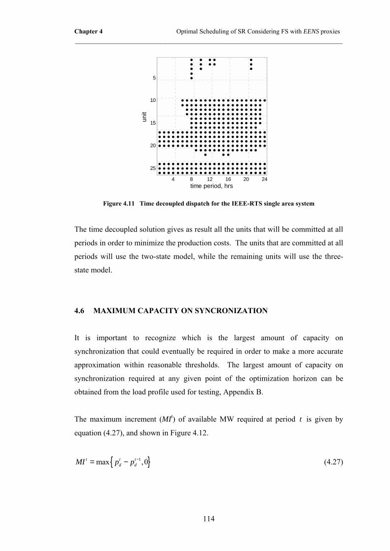
Chapter 4 Optimal Scheduling of SR Considering FS with EENS proxies ____________________________________________________________________
114
4 8 12 16 20 24
5
10
15
20
25
time period, hrs
unit
Figure 4.11 Time decoupled dispatch for the IEEE-RTS single area system
The time decoupled solution gives as result all the units that will be committed at all
periods in order to minimize the production costs. The units that are committed at all
periods will use the two-state model, while the remaining units will use the three-
state model.
4.6 MAXIMUM CAPACITY ON SYNCRONIZATION
It is important to recognize which is the largest amount of capacity on
synchronization that could eventually be required in order to make a more accurate
approximation within reasonable thresholds. The largest amount of capacity on
synchronization required at any given point of the optimization horizon can be
obtained from the load profile used for testing, Appendix B.
The maximum increment (MIt) of available MW required at period t is given by
equation (4.27), and shown in Figure 4.12.
{ }1max ,0t t td dMI p p −= − (4.27)

Chapter 4 Optimal Scheduling of SR Considering FS with EENS proxies ____________________________________________________________________
115
0 4 8 12 16 20 240
50
100
150
200
250
300
350
400
450
time period, hrs
MI,
MW
Figure 4.12 MW increment as a function of time period
The results shown in Figure 4.7 are consistent with the ones shown in Figure 4.12.
Therefore, for this system it would be necessary to calibrate the EENS approximation
to cover capacities on synchronization of up to 430 MW.
4.7 EENS BEHAVIOUR AS A FUNCTION OF THE CS
In order to approximate the EENS considering the capacity on synchronization it is
necessary to analyse its behaviour. Consider for instance the commitment at period 8
from the schedule shown in Figure 4.6. At this period the demand is 2430 MW,
Figure 4.13 shows the behaviour of the EENS as a function of the capacity on
synchronization (CS) for 100 random samples of CS. These samples are obtained by
declaring the status of the committed generators randomly, (i.e. either already
synchronized or starting-up).
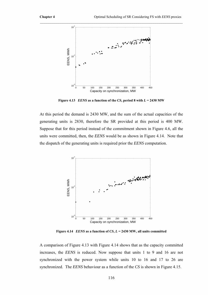
Chapter 4 Optimal Scheduling of SR Considering FS with EENS proxies ____________________________________________________________________
116
0 50 100 150 200 250 300 350 400 45010
-3
10-2
10-1
Capacity on synchronization, MW
EEN
S, M
Wh
Figure 4.13 EENS as a function of the CS, period 8 with L = 2430 MW
At this period the demand is 2430 MW, and the sum of the actual capacities of the
generating units is 2830, therefore the SR provided at this period is 400 MW.
Suppose that for this period instead of the commitment shown in Figure 4.6, all the
units were committed, then, the EENS would be as shown in Figure 4.14. Note that
the dispatch of the generating units is required prior the EENS computation.
0 50 100 150 200 250 300 350 400 45010
-3
10-2
10-1
Capacity on synchronization, MW
EEN
S, M
Wh
Figure 4.14 EENS as a function of CS, L = 2430 MW, all units committed
A comparison of Figure 4.13 with Figure 4.14 shows that as the capacity committed
increases, the EENS is reduced. Now suppose that units 1 to 9 and 16 are not
synchronized with the power system while units 10 to 16 and 17 to 26 are
synchronized. The EENS behaviour as a function of the CS is shown in Figure 4.15.

Chapter 4 Optimal Scheduling of SR Considering FS with EENS proxies ____________________________________________________________________
117
0 50 100 150 200 250 300 350 400 45010
-1
100
Capacity on synchronization, MW
EEN
S, M
Wh
Figure 4.15 EENS as a function of CS, L = 2430 MW, units committed 10 to 16 and 17 to 26
Figure 4.15 shows that the EENS increase significantly as the capacity committed is
reduces. It should also be noted from Figures 4.13 to 4.15 that as the capacity
committed increases the EENS is more spread. An approximation with an analytical
function is thus more difficult to obtain.
Figures 4.13 to 4.15 are for a single load level, but the load is an additional variable,
and the behaviour of the EENS as a function of the load level should also be taken
into consideration. Consider for instance a load level of 1690 MW and the
commitments shown in Figure 4.16.
0 50 100 150 200 250 300 35010-3
10-2
10-1
Capacity on synchronization, MW
EEN
S, M
Wh
0 50 100 150 200 250 300 350 400 450
10-6
10-5
10-4
Capacity on synchronization, MW
EEN
S, M
Wh
5 10 15 20 25Units committed
5 10 15 20 25Units committed

Chapter 4 Optimal Scheduling of SR Considering FS with EENS proxies ____________________________________________________________________
118
0 50 100 150 200 250 300 35010-3
10-2
10-1
Capacity on synchronization, MW
EE
NS
, MW
h
5 10 15 20 25Units committed
Figure 4.16 EENS as a function of the CS for different commitments, L = 1690 MW
Figure 4.16 shows that in the cases when a larger amount of units are committed, the
difference between the EENS with 0 MW on synchronization and the EENS with the
largest capacity on synchronization is smaller. This is expected, since when a larger
number of units are committed, for the same amount of capacity on synchronization,
then the probability of curtailing load in the case of a failure to synchronize of any of
the generating units is lower.
Tests with different load levels for different commitments were performed, and the
EENS behaviour as a function of the CS is similar to those presented in this section.
4.8 EENS APPROXIMATION AS A FUNCTION OF CS
The results presented in the previous section suggest that a line joining the EENS
with no CS and the EENS with the largest CS can approximate the EENS as a
function of CS. When the capacity committed in the system is much larger than the
demand to be supply, there is a large amount of SR and the convexity of the EENS as
a function of CS is pronounced. However since the values of the EENS are smaller
than in the cases where the SR is not large, the error is not significant. This line
extends from CS = 0 to CS = LCS; where LCS is the largest capacity on
synchronization. However, for a point equal or higher to LCS various combinations

Chapter 4 Optimal Scheduling of SR Considering FS with EENS proxies ____________________________________________________________________
119
of units can result in the same CS. The CS associated with the largest EENS is
preferred in order to consider the worst case. Thus, such combination of units must
have the following characteristics:
To be as close to LCS as possible: This characteristic is desirable in order to increase
the accuracy of the approximation
Smallest number of units: This characteristic is desirable because when the number
of units committed is small the units would be more heavily loaded, and therefore
the outage of a generating unit would be associated with a larger amount of load
curtailment
Most unreliable units: In the case in which two sets of units with the same CS and
the same number of units are found, the one with the less reliable units should be
selected in order to get the largest EENS
Identifying this combination with certainty is difficult because of the vast number of
combinations. Instead an auxiliary optimization searches among the eligible
combinations the one that minimizes the following objective function:
( )1 2 31 1 1
min 1Nc Nc Nc
i i i i ii i i
C pfβ σ β σ β σ= = =
+ + − ∑ ∑ ∑ (4.28)
Subject to:
1
N
i ii
AC LCSσ=
≥∑ (4.29)
i iu iσ ≤ ∀ ∈ N (4.30)
0j j buσ = ∀ ∈ (4.31)
Where:
1,2,3β weighting factors to give priorities to objectives

Chapter 4 Optimal Scheduling of SR Considering FS with EENS proxies ____________________________________________________________________
120
[ ]1,0iσ ∈ this binary variable specifies whether unit i should started
[ ]1,0iu ∈ binary variable for unit i, (1:committed, 0:decommited)
iAC available capacity of unit i
N Set of generating units
bu set of base units (units that are committed at all periods)
The results of applying the auxiliary optimization and computing the linear
approximation for a demand of 2430 MW and 1690 MW are shown in Figure 4.17
and Figure 4.18.
0 50 100 150 200 250 300 350 400 45010-3
10-2
10-1
Capacity on synchronization, MW
EE
NS
, MW
h
Actual value Approximation
0 50 100 150 200 250 300 350 400 45010-3
10-2
10-1
Capacity on synchronization, MW
EE
NS
, MW
h
Actual valueApproximation
5 10 15 20 25Units committed
5 10 15 20 25Units committed
0 50 100 150 200 250 300 350 400 45010-1
100
Capacity on synchronization, MW
EE
NS
, MW
h
Actual valueApproximation
5 10 15 20 25Units committed
Figure 4.17 EENS as a function of CS approximation for different commitments and L = 2430 MW

Chapter 4 Optimal Scheduling of SR Considering FS with EENS proxies ____________________________________________________________________
121
0 50 100 150 200 250 300 350 400 45010-3
10-2
10-1
Capacity on synchronization, MW
EE
NS
, MW
h
Actual valueApproximation
0 50 100 150 200 250 300 350 400 45010-6
10-5
10-4
Capacity on synchronization, MW
EE
NS
, MW
h
Actual valueApproximation
5 10 15 20 25Units committed
5 10 15 20 25Units committed
0 50 100 150 200 250 300 350 400 45010-3
10-2
10-1
Capacity on synchronization, MW
EE
NS
, MW
h
Actual valueApproximation
5 10 15 20 25Units committed
Figure 4.18 EENS as a function of CS approximation for different commitments and L = 1690 MW
Figure 4.17 and Figure 4.18 show that the approximation of the EENS as a function
of the CS with a single line is fairly accurate, since the actual values of the EENS are
close to the approximation. These figures also show that the slope is not the same for
all cases, therefore the behaviour of the slope, as a function of the CC should be
investigated. Consider for instance a load level of 2430 MW, the EENS with CS = 0
MW (EENS0) is obtained as explained in Chapter 3. However, when the effect of the
unreliability of the units in synchronization is taken into account, an extra term (m
CS) must be added to the EENS0 to obtain the overall EENS. The behaviour of the
slope �m� as a function CC is shown in Figure 4.19.
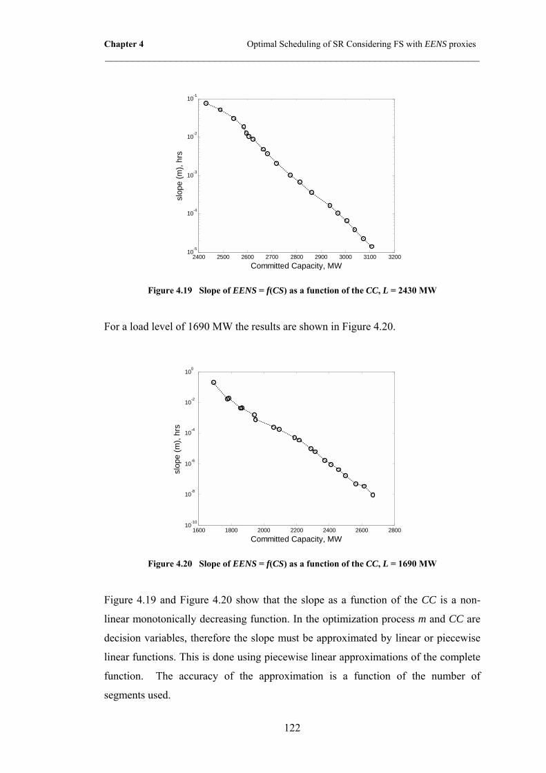
Chapter 4 Optimal Scheduling of SR Considering FS with EENS proxies ____________________________________________________________________
122
2400 2500 2600 2700 2800 2900 3000 3100 320010
-5
10-4
10-3
10-2
10-1
Committed Capacity, MW
slop
e (m
), hr
s
Figure 4.19 Slope of EENS = f(CS) as a function of the CC, L = 2430 MW
For a load level of 1690 MW the results are shown in Figure 4.20.
1600 1800 2000 2200 2400 2600 280010
-10
10-8
10-6
10-4
10-2
100
Committed Capacity, MW
slop
e (m
), hr
s
Figure 4.20 Slope of EENS = f(CS) as a function of the CC, L = 1690 MW
Figure 4.19 and Figure 4.20 show that the slope as a function of the CC is a non-
linear monotonically decreasing function. In the optimization process m and CC are
decision variables, therefore the slope must be approximated by linear or piecewise
linear functions. This is done using piecewise linear approximations of the complete
function. The accuracy of the approximation is a function of the number of
segments used.

Chapter 4 Optimal Scheduling of SR Considering FS with EENS proxies ____________________________________________________________________
123
To build the approximation it is necessary first to select the desired number of
segments and generate an array of possible CC samples. From these samples the
ones that divide the CC range in segments of almost the same length are chosen.
Figure 4.21 shows the approximation with 7 segments for a load level of 1690 MW
on logarithmic y-axis.
1600 1800 2000 2200 2400 2600 280010
-10
10-8
10-6
10-4
10-2
100
Committed Capacity, MW
slop
e (m
), hr
s
Actual valueApproximation
Figure 4.21 Approximation of the slope of EENS = f(CS) as a function of the CC for L = 1690 MW with 8 segments
The same can be applied for load level of 2430 MW, Figure 4.22.
2400 2500 2600 2700 2800 2900 3000 3100 320010
-5
10-4
10-3
10-2
10-1
Committed Capacity, MW
slop
e (m
), hr
s
Actual valueApproximation
Figure 4.22 Slope of EENS = f(CS) as a function of CC for L = 2430 MW with 8 segments

Chapter 4 Optimal Scheduling of SR Considering FS with EENS proxies ____________________________________________________________________
124
Figure 4.23 shows the curves of the slope as a function of the CC for different load
levels.
1400 1600 1800 2000 2200 2400 2600 2800 3000 320010-10
10-8
10-6
10-4
10-2
100
102
Committed Capacity, MW
slop
e (m
), hr
s
Actual valueApproximation
1500 MW
1750 MW
2000 MW
2250 MW
2500 MW
2750 MW
Figure 4.23 Slope of EENS = f(CS) as a function of the CC for various load levels
4.9 IMPLEMENTATION OF THE PROPOSED UC APPROACH
The proposed approach can be implemented using Mixed Integer Linear
Programming (MILP), details can be found in appendix C. However, to compute
the EENS at each period of the optimization horizon extra constraints are required.
For a given combination of units the EENS is function of the load to be supplied, the
committed capacity (CC) and the capacity on synchronization (CS). When
considering the CS at each period of the optimization horizon, the EENS is the sum
of two components:
• The contribution due to failure of committed units
• The contribution due to failure to synchronize of generating units starting-up

Chapter 4 Optimal Scheduling of SR Considering FS with EENS proxies ____________________________________________________________________
125
failure of alreadydue to failure committed unitsto synchronize
0t t t tEENS m CS EENS= + !"#"$!#$ (4.32)
Where mt and EENS0t are the slope and the y-offset respectively, and both are
functions of the CCt. This variable is given by the sum of the actual capacity of the
committed generating units:
1
Nt t
ii
CC AC=
=∑ (4.33)
CSt represents the capacity on synchronization at each period of the optimization
horizon. In order to obtain this variable it is necessary to identify separately the units
that are being synchronized by a single binary variable ( tius ), details of the
representation of this table with linear constraints are in appendix C:
Table 4.2 Possible states for the auxiliary constraints
tiu 1t
iu − tius
0 0 0
0 1 0
1 0 1
1 1 0
Once this variable is obtained, then the capacity of a unit starting-up at period t is
given by:
t t ti i iACS AC us= (4.34)
Equation (4.34) is clearly non-linear; therefore it has to be replaced by linear
constraints as explained in (Williams, 1999, Guéret et al., 2000):
t ti iACS AC≤ (4.35)

Chapter 4 Optimal Scheduling of SR Considering FS with EENS proxies ____________________________________________________________________
126
( )max 1t t ti i i iACS AC P us≥ − − (4.36)
maxt t
i i iACS us P≤ (4.37)
The sum of the capacities synchronizing at each period of the optimization horizon
results in the total capacity on synchronization:
1
Nt t
ii
CS ACS=
=∑ (4.38)
As explained before, the value of EENS0t is the EENSt when CSt = 0 MW, then this
value can be approximated in a piecewise fashion as explained in Chapter 3, by
means of using special ordered sets 2 (SOS2), (Williams, 1999). Since mt as a
function of CCt is approximated in the same fashion as EENS0t, then a similar set of
equations to the ones used to obtain the values of EENS0t is used to compute the
value of the slope (mt). However, the number of elbow points can be different,
therefore in this case it is assumed that the piecewise linear approximation is defined
by the x- and y-coordinates ( tgXcs , t
gYcs ) of the �G� elbow points, with 1,...,g G= .
The variables tm and tCS are decision variables since they depend on the
scheduling at a given period of the optimization horizon. However, these two
variables are real variables. This product is clearly non-linear and cannot be
implemented directly into the MIP engine. Figure 4.12 shows that tCS vary in the
range of [0, 430] MW, and Figure 4.23 shows that the tm varies in the range [1×10⁻⁹,
1] hrs. The product t tm CS is shown in Figure 4.24.
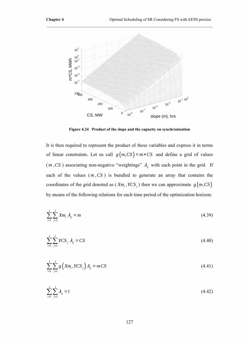
Chapter 4 Optimal Scheduling of SR Considering FS with EENS proxies ____________________________________________________________________
127
10-910-7
10-510-3 10-1 100
0100
200300
400430
10-7
10-5
10-3
10-1100
102
slope (m), hrsCS, MW
m*C
S, M
Wh
Figure 4.24 Product of the slope and the capacity on synchronization
It is then required to represent the product of these variables and express it in terms
of linear constraints. Let us call ( ),g m CS m CS= × and define a grid of values
( m ,CS ) associating non-negative �weightings� ijλ with each point in the grid. If
each of the values ( m ,CS ) is bundled to generate an array that contains the
coordinates of the grid denoted as ( iXm , jYCS ) then we can approximate ( ),g m CS
by means of the following relations for each time period of the optimization horizon:
1 1
I J
i iji j
Xm mλ= =
=∑∑ (4.39)
1 1
I J
j iji j
YCS CSλ= =
=∑∑ (4.40)
( )1 1
,I J
i j iji j
g Xm YCS mCSλ= =
=∑∑ (4.41)
1 1
1I J
iji j
λ= =
=∑∑ (4.42)

Chapter 4 Optimal Scheduling of SR Considering FS with EENS proxies ____________________________________________________________________
128
In addition to the previous constraints, it would be necessary to impose the
restriction that at most four neighbouring λs can be non-zero. We can impose this
last condition in the following way; let:
1
J
i ijj
ξ λ=
=∑ 1,...,i I∀ = (4.43)
1
I
j iji
η λ=
=∑ 1,...,j J∀ = (4.44)
Each of the sets generated by equations (4.43) and (4.44) are ( )1,..., Iξ ξ and
( )1,..., Jη η respectively. These sets should be handled as further SOS2. The SOS2
condition for the first set allows λs to be non-zeros in at most two neighbouring
columns, Figure 4.25 and Figure 4.26.
11
23
1
tt
t
tIt
I
d
d
ξξ
ξ −
≤
M %%
(4.45)
1
11
Itk
kd
−
=
=∑ (4.46)
Where: 3M is a ( )1I I× − matrix constructed in a similar way as explained for the
adjacency conditions of the piecewise approximation of EENS0. tkd is a binary
variable such that 1tkd = if mt lays within segment �k� and 0t
kd = otherwise.
For the second set, the SOS2 condition allows λs to be non-zero in at most two
neighbouring rows, Figure 4.25 and Figure 4.26.
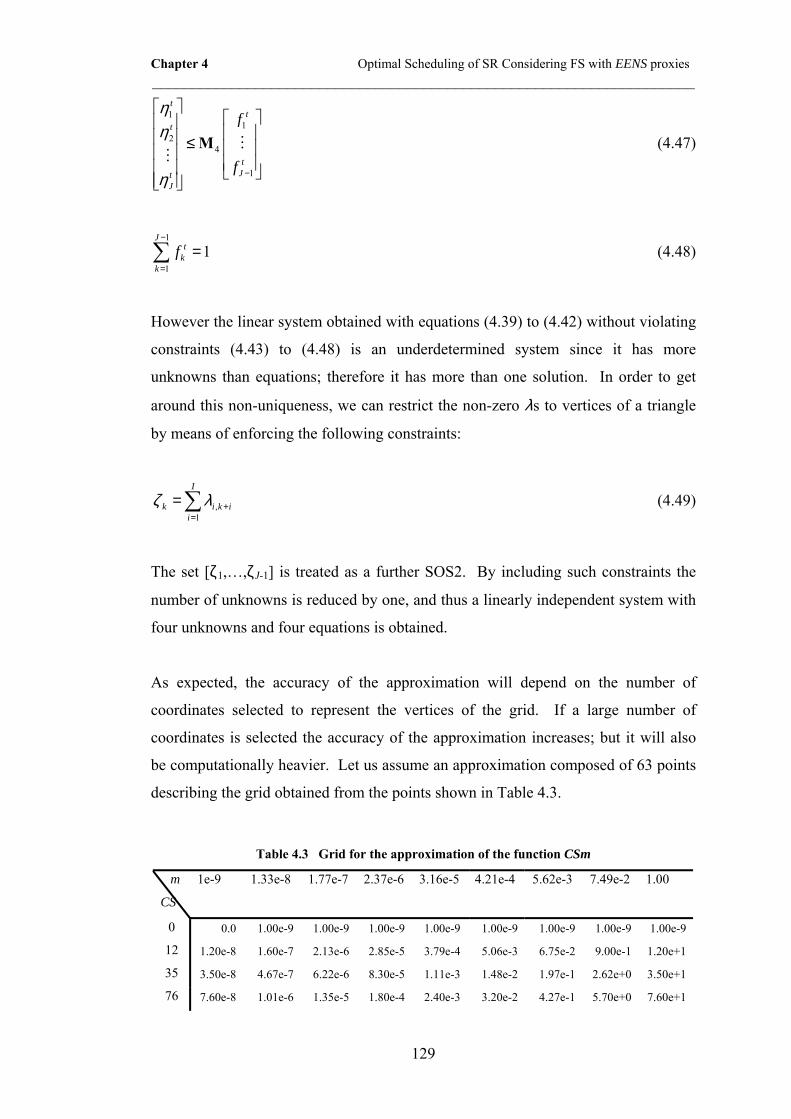
Chapter 4 Optimal Scheduling of SR Considering FS with EENS proxies ____________________________________________________________________
129
11
24
1
tt
t
tJt
J
f
f
ηη
η −
≤
M %%
(4.47)
1
11
Jt
kk
f−
=
=∑ (4.48)
However the linear system obtained with equations (4.39) to (4.42) without violating
constraints (4.43) to (4.48) is an underdetermined system since it has more
unknowns than equations; therefore it has more than one solution. In order to get
around this non-uniqueness, we can restrict the non-zero λs to vertices of a triangle
by means of enforcing the following constraints:
,1
I
k i k ii
ζ λ +=
=∑ (4.49)
The set [ζ1,�,ζJ-1] is treated as a further SOS2. By including such constraints the
number of unknowns is reduced by one, and thus a linearly independent system with
four unknowns and four equations is obtained.
As expected, the accuracy of the approximation will depend on the number of
coordinates selected to represent the vertices of the grid. If a large number of
coordinates is selected the accuracy of the approximation increases; but it will also
be computationally heavier. Let us assume an approximation composed of 63 points
describing the grid obtained from the points shown in Table 4.3.
Table 4.3 Grid for the approximation of the function CSm
m
CS 1e-9 1.33e-8 1.77e-7 2.37e-6 3.16e-5 4.21e-4 5.62e-3 7.49e-2 1.00
0 0.0 1.00e-9 1.00e-9 1.00e-9 1.00e-9 1.00e-9 1.00e-9 1.00e-9 1.00e-9
12 1.20e-8 1.60e-7 2.13e-6 2.85e-5 3.79e-4 5.06e-3 6.75e-2 9.00e-1 1.20e+1
35 3.50e-8 4.67e-7 6.22e-6 8.30e-5 1.11e-3 1.48e-2 1.97e-1 2.62e+0 3.50e+1
76 7.60e-8 1.01e-6 1.35e-5 1.80e-4 2.40e-3 3.20e-2 4.27e-1 5.70e+0 7.60e+1

Chapter 4 Optimal Scheduling of SR Considering FS with EENS proxies ____________________________________________________________________
130
155 1.55e-7 2.07e-6 2.76e-5 3.68e-4 4.90e-3 6.54e-2 8.72e-1 1.16e+1 1.55e+2
300 3.00e-7 4.00e-6 5.33e-5 7.11e-4 9.49e-3 1.27e-1 1.69 2.25e+1 3.00e+2
430 4.30e-7 5.73e-6 7.65e-5 1.02e-3 1.36e-2 1.81e-1 2.42 3.22e+1 4.30e+2
Figure 4.25 shows the values of Table 4.3 with its associated weighting variable λ.
10-9
10-7
10-5
10-3 10-1 100
0100
200300
400430
10-7
10-5
10-3
10-1100
102
λ91λ81
λ92
λ93
λ94
λ71
λ82
λ83
λ84
λ61
λ72
λ95
λ73
λ74
λ51
λ62
λ85
λ63
λ64
λ41
λ52
λ75
λ96
slope (m), hrs
λ53
λ54
λ31
λ42
λ65
λ86
λ43
λ44
λ97
λ21
λ32
λ55
λ76
λ33
λ34
λ87
λ22
λ45
λ66
λ23
λ11
λ24
λ77
λ12
λ35
λ56
λ13
λ14
λ67
λ25
λ46
λ57
λ15
λ36
λ47
CS, MW
λ26
λ37
λ16
λ27
λ17
m*C
S, M
Wh
Figure 4.25 Approximation of the non-linear function with 42 grid points
The position of each of the weighting variables is shown in a 2D plot, Figure 4.26.
10-10
10-8
10-6
10-4
10-2
100
0
50
100
150
200
250
300
350
400
450
λ11λ12
λ13
λ14
λ15
λ16
λ17
λ21λ22
λ23
λ24
λ25
λ26
λ27
λ31λ32
λ33
λ34
λ35
λ36
λ37
λ41λ42
λ43
λ44
λ45
λ46
λ47
λ51λ52
λ53
λ54
λ55
λ56
λ57
λ61λ62
λ63
λ64
λ65
λ66
λ67
λ71λ72
λ73
λ74
λ75
λ76
λ77
λ81λ82
λ83
λ84
λ85
λ86
λ87
λ91λ92
λ93
λ94
λ95
λ96
λ97
slope (m), hrs
CS
, MW
Figure 4.26 Position of the weighting variables

Chapter 4 Optimal Scheduling of SR Considering FS with EENS proxies ____________________________________________________________________
131
Let us suppose a hypothetical case in which the system is serving a load level of
2430 MW with a CC = 2771.3 MW, then m = 0.0011853 hrs, and if the CS = 310
MW, then making the direct product of these variables we get: mCS = 0.36744
MWh. Doing it using equations (4.39) to (4.49) we get the following linear system:
6 6 7 66
6 7 6 67
6 6 6 7 7 6 76
001 0
1 1 1 0 1
Xm Xm Xm mYCS YCS YCS CS
Xm YCS Xm YCS Xm YCSmCS
λλλ
= −
(4.50)
This linear system gives: mCS = 0.35981 MWh which is close to the actual value
obtained by multiplying m and CS. However the accuracy is proportional to the
number of grid points selected in the approximation.
4.10 TEST RESULTS
The proposed UC formulation was tested on the IEEE-RTS single-area system and
the IEEE-RTS three-area system.
4.10.1 Test Results in the IEEE-RTS Single-Area System
The proposed UC formulation was tested on the IEEE-RTS one area system without
hydro generation, Appendix B. Optimizations were performed using a branch and
bound technique coded in XpressMP (Dash Associates, 2005), and a MIP gap no
larger than 0.16% was considered adequate. The load profile used for testing is the
same as in Chapter 3.
Figure 4.27 shows the scheduling computed by the different UC formulations. Case
A shows the UC enforcing the traditional SR constraint with ( )maxmaxt td i ir u P= .
Case B shows the scheduling enforcing the constraints to include the EENS cost
without considering the failure to synchronize using a VOLL of 4,000 $/MWh.

Chapter 4 Optimal Scheduling of SR Considering FS with EENS proxies ____________________________________________________________________
132
Finally case C shows the scheduling enforcing the constraints to include the EENS
cost including the failure to synchronize for VOLL = 4,000 $/MWh.
4 8 12 16 20 24
5
10
15
20
25
time period, hrs
unit
a) Traditional UC formulation
4 8 12 16 20 24
5
10
15
20
25
time period, hrs
unit
b) Proposed UC formulation including the EENS cost, VOLL = 4,000 $/MWh
4 8 12 16 20 24
5
10
15
20
25
time period, hrs
unit
c) Proposed UC formulation including the EENS cost with the FS, VOLL = 4,000 $/MWh
Figure 4.27 Comparison of different scheduling formulations
At the light load periods, the capacity on synchronization does not play a key role in
the total cost of the scheduling since the slope of the approximation is quite small
compared with the slope obtained for the cases of heavier load; therefore at the light
load periods there can be significant amount of capacity on synchronization not
increasing considerably the EENS. On the other hand, as the load increases, the
capacity on synchronization would have a larger impact on the EENS at such periods
since losing any of the synchronizing units would be more likely to result in an

Chapter 4 Optimal Scheduling of SR Considering FS with EENS proxies ____________________________________________________________________
133
energy curtailment. This explains the results shown in Figure 4.27, since apparently
the scheduling with the two proposed formulations are similar; however the one that
includes the failure to synchronize schedules the units 6 to 9 differently. Table 4.4
shows the itemized costs of each of the formulations.
Table 4.4 Cost for each of the UC formulations
UC formulation Traditional, $ EENS, $ EENS with FS, $
Start-up cost 4,466.00 4,466.00 4,524.00
Dispatch cost 736,424.83 736,205.41 735,989.20
EENS cost 597.95 634.14 731.45
Total cost 741,488.78 741,310.55 741,244.65
Table 4.4, shows that the proposed UC formulation considering the failure to
synchronize is cheaper in the overall compared with the traditional formulation and
the proposed formulation considering only the EENS cost.
The cases for the traditional UC approach and the proposed UC approach
considering the EENS and neglecting the failures to synchronize are the ones in
which the solutions are obtained with a lower MIP gap, (lower than 0.075%), while
the case in which the failures to synchronize are considered, the MIP gap was never
lower than 0.16% and it never converged to an optimal solution even leaving it
running for long periods of time (hours). It is then recognized that the computational
burden demanded by the proposed UC formulation considering failures to
synchronize is higher than the required by either the traditional UC formulation or
the proposed UC formulation considering the EENS cost alone. This is because the
model to include the product of the capacity on synchronization and the slope turns
out to be too cumbersome and hinders the ability of the optimization procedure to
reach the optimum.
Figure 4.28 and Figure 4.29 show the total cost for different UC approaches and
different deterministic reserve criteria. In these figures the overall costs have been
normalized using as a basis the sum of the running and start-up costs for the
traditional UC and the standard rule-of-thumb for the reserve requirement (in this

Chapter 4 Optimal Scheduling of SR Considering FS with EENS proxies ____________________________________________________________________
134
case rdt = 400 MW). Similarly, VOLL has been normalized on the basis of the
average cost of electrical energy for the same UC case (13.493 $/MWh), the x-scale
is logarithmic in order to highlight the differences between the two formulations for
low VOLLs.
101 102 103 1040.97
0.975
0.98
0.985
0.99
0.995
1
1.005
1.01
1.015
VOLL, p.u.
tota
l cos
t, p.
u.
traditional, rdt = 400 MW
with EENS cost with FSwith EENS cost
Figure 4.28 Normalized total costs as a function of the normalized VOLL for the different UC formulations
Two different deterministic criteria are used and the results are:
101 102 103 1040.97
0.975
0.98
0.985
0.99
0.995
1
1.005
1.01
1.015
VOLL, p.u.
tota
l cos
t, p.
u.
traditional, rdt = 420 MW
with EENS cost with FSwith EENS cost
a) Comparison against a rdt = 420 MW
101 102 103 1040.96
0.98
1
1.02
1.04
1.06
1.08
VOLL, p.u.
tota
l cos
t, p.
u.
traditional, rdt = 380 MW
with EENS cost with FSwith EENS cost
b) Comparison against a rdt = 380 MW
Figure 4.29 Normalized costs as a function of the Normalized VOLL for different UC formulations and different deterministic criteria

Chapter 4 Optimal Scheduling of SR Considering FS with EENS proxies ____________________________________________________________________
135
4.10.2 Test Results in the IEEE-RTS Three-Area System
The IEEE-RTS96 three-area system without hydro generation as in Chapter 3 has
been used to test the proposed formulation. Optimizations were performed using the
same branch and bound technique as before, and a MIP gap no larger than 0.15%
was considered adequate. The load profile used for testing is the same as in Chapter
3.
Applying the time decoupled base commitment with economic dispatch the solution
of the system is as follows:
6 12 18 24 30 36 42 48 54 60 66 72 78
4
8
12
16
20
24
unit
time
perio
d, h
rs
Figure 4.30 Time decoupled base commitment with economic dispatch for the IEEE-RTS three-area system
From the previous figure it can be appreciated that the base units are: [49 50 51 52
53 54 55 56 57 70 71 72 73 74 75 76 77 78], for the given load profile.
Applying equation (4.27) the load increments for each time period are obtained.

Chapter 4 Optimal Scheduling of SR Considering FS with EENS proxies ____________________________________________________________________
136
0 4 8 12 16 20 240
200
400
600
800
1000
1200
time period, hrs
MI,
MW
Figure 4.31 MW increment as a function of the time period for the load pattern used for testing
From the previous figure it can be appreciated that the maximum MW increment is
of 1121 MW at period 7; therefore the maximum capacity on synchronization can be
assumed to be 1130 MW. As shown in Figure 4.23, the maximum and the minimum
slope of EENS = f(CS) are associated with the minimum load level to serve in the
system in the system, which in this case is 4726 MW. The slope EENS = f(CS) as a
function of the committed capacity for this load level is shown in Figure 4.32.
4500 5000 5500 6000 6500 7000 750010-20
10-15
10-10
10-5
100
Committed Capacity, MW
slop
e (m
), hr
s
Figure 4.32 Slope of EENS = f(CS) as a function of the committed capacity for L = 4726 MW
As in the case of the single area system if 42 grid points are used to approximate the
non linear function this would look as shown in Figure 4.33 with a range of [1×10-14,

Chapter 4 Optimal Scheduling of SR Considering FS with EENS proxies ____________________________________________________________________
137
0.1] hrs for the slope of EENS = f(CS), and [0, 1130] MW for the capacity on
synchronization.
10-12
10-9
10-6
10-3
0200
400600
8001000
10-10
10-5
100
λ91
λ92
λ93
λ94
λ81
λ82
λ83
λ84
λ71
λ72
λ95
λ73
λ74
λ61
λ62
λ85
λ63
λ64
λ51
λ52
λ75
λ96
slope (m), hrs
λ53
λ54
λ41
λ42
λ65
λ86
λ43
λ44
λ31
λ32
λ97
λ55
λ76
λ33
λ34
λ21
λ22
λ87
λ45
λ66
λ23
λ24
λ11
λ12
λ77
λ35
λ56
λ13
λ14
λ67
λ25
λ46
λ57
λ15
λ36
λ47
CS, MW
λ26
λ37
λ16
λ27
λ17
m*C
S, M
Wh
Figure 4.33 Product of the capacity on synchronization and the slope
The results of the traditional UC formulation with rdt = 400 and the proposed UC
formulations are shown in Figure 4.34.
101 102 103 1040.995
1
1.005
1.01
1.015
1.02
1.025
VOLL, p.u.
tota
l cos
t, p.
u.
traditional, rd = 400 MW
with EENS costwith EENS cost with FS
Figure 4.34 Normalized total costs as a function of the normalized VOLL
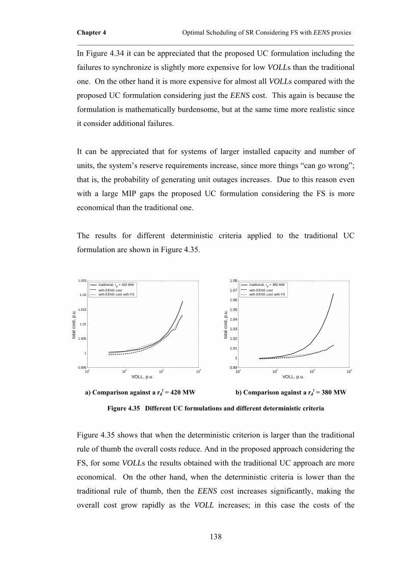
Chapter 4 Optimal Scheduling of SR Considering FS with EENS proxies ____________________________________________________________________
138
In Figure 4.34 it can be appreciated that the proposed UC formulation including the
failures to synchronize is slightly more expensive for low VOLLs than the traditional
one. On the other hand it is more expensive for almost all VOLLs compared with the
proposed UC formulation considering just the EENS cost. This again is because the
formulation is mathematically burdensome, but at the same time more realistic since
it consider additional failures.
It can be appreciated that for systems of larger installed capacity and number of
units, the system�s reserve requirements increase, since more things �can go wrong�;
that is, the probability of generating unit outages increases. Due to this reason even
with a large MIP gaps the proposed UC formulation considering the FS is more
economical than the traditional one.
The results for different deterministic criteria applied to the traditional UC
formulation are shown in Figure 4.35.
101 102 103 1040.995
1
1.005
1.01
1.015
1.02
1.025
VOLL, p.u.
tota
l cos
t, p.
u.
traditional, rd = 420 MW
with EENS costwith EENS cost with FS
a) Comparison against a rdt = 420 MW
101 102 103 1040.99
1
1.01
1.02
1.03
1.04
1.05
1.06
1.07
1.08
VOLL, p.u.
tota
l cos
t, p.
u.
traditional, rd = 380 MW
with EENS costwith EENS cost with FS
b) Comparison against a rdt = 380 MW
Figure 4.35 Different UC formulations and different deterministic criteria
Figure 4.35 shows that when the deterministic criterion is larger than the traditional
rule of thumb the overall costs reduce. And in the proposed approach considering the
FS, for some VOLLs the results obtained with the traditional UC approach are more
economical. On the other hand, when the deterministic criteria is lower than the
traditional rule of thumb, then the EENS cost increases significantly, making the
overall cost grow rapidly as the VOLL increases; in this case the costs of the

Chapter 4 Optimal Scheduling of SR Considering FS with EENS proxies ____________________________________________________________________
139
proposed UC formulations are lower than the traditional, because both approaches
schedules a larger amount of SR to reduce the EENS costs.
4.11 CONCLUSIONS
This Chapter presents a new unit commitment formulation that includes a more
complete reliability model of the generating units. This model considers not only the
probability of the units undergoing to outage, but also the probability of unsuccessful
synchronizations with the power system.
This proposed unit commitment approach optimizes both, the operating costs of the
power system (start-up and dispatch costs) and the expected cost of unserved energy
due to generating units� outages and failures to synchronize. While in principle this
approach works because it provides a better balance between the cost of providing
spinning reserve and the benefits derived from such reserve, it is mathematically
burdensome. This mathematical burden results in a long time to reach integer
solutions and large MIP gaps.
For low VOLLs, in a small system this proposed approach results in better solutions
than the traditional UC formulation, but not in better solutions than the proposed UC
formulation considering just the EENS cost without FS. On the other hand, for large
systems with a large VOLL this approach is more likely to find a better solution than
the traditional UC approaches.

Chapter 5 Optimizing the Spinning Reserve Requirements ____________________________________________________________________
140
Chapter 5
Optimizing the Spinning Reserve Requirements
5.1 INTRODUCTION
In Chapter 1 and 2 it was pointed out that a common criterion for setting the
minimum amount of Spinning Reserve (SR) requirement is that it should be greater
or equal than the capacity of the largest online generator (Wood and Wollenberg,
1996). It was shown that this criterion ensures that no load would have to be
curtailed in the case of the outage of any single generating unit but that it does not
guarantee such a positive outcome if two generating units trip almost
simultaneously. It was also mentioned that increasing the SR requirement using a
similarly simple criterion would reduce the probability of an unprotected
contingency and, at the same time, lower the overall level of risk at which the power
system is operating. However, providing SR has a cost because it requires
committing additional generating units and/or operating others at less than optimal
output. Power system operators should therefore not only schedule generating units
to minimize the cost of providing the required SR, but also determine what this
requirement should be to achieve the optimal level of risk.
In Chapter 1 it was also listed the methods used to schedule SR. These methods can
be categorized under the following headings:
• Methods that directly enforce the SR requirements constraint: These methods
use the traditional unit commitment (UC) formulation; however, the SR
requirements are tailored and set to attain an specific level of risk in each

Chapter 5 Optimizing the Spinning Reserve Requirements ____________________________________________________________________
141
power system, (Wood and Wollenberg, 1996, REE, 1998, IESO, 2004, PJM,
2004, UCTE, 2005, CAISO, 2005).
• Enforcing the SR requirements using a risk proxy: Instead of explicitly
selecting a fixed amount of SR, these methods set a risk target to attain at
each period. However, the risk level depends on the demand to serve, the
units committed and their individual availability; thus, these methods have to
include a tractable way to estimate this risk for any combinations of units and
any load level, (Chattopadhyay and Baldick, 2002, Bouffard and Galiana,
2004).
• Online SR optimization: These methods include the expected cost of outages
within the objective function. Thus, the objective function combines
conflicting objectives. On the one hand, it minimizes the operating costs, that
is, the production costs and start-up costs, (it should be noted that reducing
the SR provision reduces this cost), on the other hand, it also minimizes the
EENS cost, (increasing the SR provision reduces this cost). Therefore, these
techniques procure SR up to the point where more or less SR provision
results in a higher overall cost, (Ortega-Vazquez et al., 2006, forthcoming,
Bouffard et al., 2005a, Bouffard et al., 2005b).
Setting arbitrary levels of SR and/or risk to attain at each period of the optimization
horizon hinders the ability of the optimization process to attain an overall optimum.
This is because while the SR requirements and/or risk level to attain are optimal at
one period, they might be insufficient or excessive at others, as pointed out in
Chapters 1 and 2. On the other hand, by means of including the expected cost of
outages explicitly in the objective function the results are optimal. However, the
main problem with this approach is that there is no direct means of including the full
expected energy not served distribution within the optimization process while
keeping it tractable. Thus, these approaches have to either include proxies or truncate
the outage calculation in order to avert a combinatorial explosion.
While the method described in the Chapter 3 optimizes the SR provision as part of
the UC solution process, the method proposed in this chapter determines the optimal
SR requirement for each period of the optimization horizon prior to the UC solution.

Chapter 5 Optimizing the Spinning Reserve Requirements ____________________________________________________________________
142
The benefit derived from the provision of SR is balanced against an estimate of the
cost of providing this SR. The benefit is measured by the reduction in the expected
socio-economic cost of supply interruptions to consumers achieved through the
provision of SR (EENS cost, which is computed as explained in subsection 2.4).
Instead of using some general criterion, both the benefit and the cost are recalculated
before each UC solution based on the cost and reliability characteristics of the
generating units that are likely to be scheduled to provide energy and SR. The
optimization of the SR requirement is thus decoupled from the optimization of the
generation schedule. Once the optimal SR requirement has been determined for each
hour, this value is used in the standard SR constraints of a conventional UC. This
method is described in more details in the following section.
5.2 PROPOSED APPROACH DESCRIPTION
Two parts compose the complete methodology; first the optimal SR requirements are
computed in a time-decoupled fashion, and then these optimal SR requirements are
fed to a conventional UC program and the solution is computed considering the
inter-temporal couplings and ramp-rate limitations of the generating units. Figure 5.1
shows schematically the proposed approach.
Optimal SRrequirements
Initialization
UnitCommitment
t = T?
t = t +1
No
Yes
.
Optimal SRrequirements
Initialization
UnitCommitment
t = T?
t = t +1
No
Yes
.
Figure 5.1 Unit commitment with optimal SR assessment

Chapter 5 Optimizing the Spinning Reserve Requirements ____________________________________________________________________
143
In the initialization section, the relevant information of the power system is gathered
(i.e. start-up costs, production costs, units’ constraints, units availabilities, etc.) as
well as the load forecast for the optimization horizon. Then, for each period of the
optimization horizon the optimal SR requirement is computed. Once the optimal SR
requirements are computed for all periods, this information is fed to the UC
optimization in order to find a solution considering all the intertemporal constraints.
The next subsections describe in more details each of the main blocks of the
proposed approach.
5.2.1 Optimal SR Requirements
In Chapter 1 it was mentioned that as the amount of SR scheduled increases, the
system operating cost increases while the socio-economic cost associated with the
EENS decreases because the probability of shedding load in response to unforeseen
outages of generating units is reduced. The optimal amount of SR is the amount that
minimizes the sum of these two costs. This minimum, however, is a complex
function not only of the amount of SR but also of the load and of the particular
combination of units used to meet that load. This combinatorial dependence gives
the function a number of local minima that must be distinguished from the global
optimum.
Ideally the optimization of the SR requirements should be carried out considering the
entire optimization horizon in order to take into account the start-up costs and the
inter-temporal constraints on the generating units. This would require the calculation
of the EENS cost within the UC. Such a calculation would require the calculation of
the whole discrete capacity outage probability distribution for a vast number of
combinations of generating units. That calculation is considerably beyond what is
currently achievable with a reasonable amount of computing resources.
To overcome this problem, the optimal SR requirement is calculated separately for
each load level of the scheduling horizon using an auxiliary optimization. This
auxiliary optimization determines the SR requirement that minimizes the sum of the
commitment-dispatch and EENS costs for a given load level. Thus, this optimization
process combines two conflicting objectives. Furthermore, the cost minimization of
the SR procurement requires itself the commitment-dispatch solution, therefore it

Chapter 5 Optimizing the Spinning Reserve Requirements ____________________________________________________________________
144
can be established as a layered optimization problem, (Alexandrov and Dennis,
1994). Since this calculation considers each UC period separately, it is quite fast and
the only approximation is that it neglects the effect that inter-temporal constraints
might have on the reserve requirements.
Formally, this auxiliary optimization problem at period t is expressed as follows:
( ) ( ) ( ){ }mintd
t t td d dr
f r D r E r= + (5.1)
Where tdr is the amount of spinning reserve required at period t ; ( )t
dD r is the
running cost of serving the demand and procuring the amount of SR tdr and ( )t
dE r is
the EENS cost for the given scheduling.
5.2.1.1 Running Cost
For a given SR requirement, the running cost for each load level must be minimized
with respect to the committed units and their dispatch using a single period UC:
( ) ( ), 1
min ,t ti i
Nt t t
d i i iu p iD r c u p
=
= ∑ (5.2)
Subject to the load/generation balance and reserve constraints:
10
Nt t td i i
ip u p
=
− =∑ (5.3)
10
Nt t
d ii
r r=
− =∑ (5.4)
The dispatch of the generating units is also constrained by their minimum and
maximum generating limits.

Chapter 5 Optimizing the Spinning Reserve Requirements ____________________________________________________________________
145
Even being a time decoupled UC solution; the ramp-up limits of the generating
units’ must be taken into account in order to guarantee that effectively the amount of
SR tdr is being procured. This amount of SR is the sum of the individual
contributions of the generating units:
( ) ( ){ }max upmin ,t t t ti i i i i ir u P p u Rτ= − (5.5)
5.2.1.2 EENS Cost
The socio-economic cost of a particular supply interruption is defined as the product
of the Energy Not Supplied (ENS) during this interruption and a VOLL determined
using a survey (Kariuki and Allan, 1996, Lawton et al., 2003). Since it is impossible
to predict how much (or even whether any) load will have to be shed during the
implementation of a particular generation schedule, only an expected cost can be
computed. The EENS cost is thus given by:
( )t tdE r VOLL EENS= × (5.6)
Where tEENS is the Expected Energy Not Served that would result from the
generation schedule at period t . A technique for computing EENS is described in
(Billinton and Allan, 1996) and cited in section 2.4.
Figure 5.2 illustrates this auxiliary optimization for the IEEE-RTS single-area
system (Grigg et al., 1999). If the hydro generating units are omitted, this system
consists of 26 units with a total generation capacity of 3105 MW. The quadratic
approximation of the cost functions and ramp-up limits were taken from (Wang and
Shahidehpour, 1993). For more details of this test system refer to Appendix B. A
load level of 1690 MW and a VOLL = 1,000 $/MWh were assumed. As the SR
requirement increases, the dispatch cost increase while the EENS cost decreases.
The curve that shows the sum of these two costs exhibits a global minimum at the
optimal amount of SR.

Chapter 5 Optimizing the Spinning Reserve Requirements ____________________________________________________________________
146
100 200 300 4001.87
1.88
1.89
1.9x 10⁴
Spinning Reserve, MW
tota
l cos
t, $
100 200 300 4001.82
1.84
1.86
1.88
1.9x 10⁴
Spinning Reserve, MWdi
spat
ch c
ost,
$100 200 300 4000
200
400
600
800
Spinning Reserve, MW
EEN
S c
ost,
$
+
=
Figure 5.2 Dispatch, EENS and total costs for the IEEE-RTS for L = 1690 MW and VOLL =
1,000 $/MWh
A number of search-based techniques have been developed to solve efficiently such
univariate optimization problems. However, in this case, the total cost curve is
essentially unimodal but non-convex because the dispatch cost changes suddenly
every time an additional and more expensive unit needs to be committed to meet the
SR requirement. The search technique should therefore be able to avoid getting
trapped in a local minimum. Furthermore, the number of cost calculations should be
kept small because each evaluation requires one single-period unit commitment and
the calculation of the corresponding COPT. Among the various search techniques
that have been developed to solve this type of optimization problem, the iterated grid
search with three grid points, (Kim, 1997) provides a good compromise between
speed, robustness and accuracy. Some other techniques such as Fibonacci search and
the golden search were tested, however, the three-point grid search was preferred
because it recycles one search point at each iteration, and having three points gives a
better indication of the behaviour of the function. This technique is described in
more details in the following subsection.
5.2.2 Three-Point Grid Search
The following steps describe a grid search algorithm using three test points at every
iteration step:

Chapter 5 Optimizing the Spinning Reserve Requirements ____________________________________________________________________
147
1. Select an acceptable length of uncertainty “ err ”, that is, a maximum
span of SR in which the solution is contained.
2. At the first iteration ( 1k = ) select the interval of SR in which the
solution is contained (i.e. an upper and lower bounds for the search),
[ ],kI Lb Ub= .
3. If the difference between the upper and lower bounds is smaller than a
defined length of uncertainty ( ( )Ub Lb err− < ), then the minimum
cost lies in the span [ ],Lb Ub .
4. Select 3 test points ,1 ,2 ,3, ,d d d kr r r I∈ such that
,1 ,2 ,3d d dLb r r r Ub≤ ≤ ≤ ≤ , then the set of values
( ) ( ) ( ),1 ,2 ,3, ,d d df r f r f r , gives some indication of the behaviour of
( )df r . Since the shape of ( )df r is unknown, it is suggested that the
test points are equidistant, then, they can be computed as:
( ), 1, 2,34d mmr Lb Ub Lb m= + − ∀ = (5.7)
5. If 1k < check for the values of ,d mr at 1k − that repeat at k in order
to avert the evaluation of ( )df r .
6. Let Sk be the set of values of ( )df r evaluated at each test point, thus,
( ) ( ) ( ){ },1 ,2 ,3, ,k d d dS f r f r f r= .
Lb Ubrd,1
A B C D
rd,2 rd,3Lb Ubrd,1
A B C D
rd,2 rd,3
Figure 5.3 Equidistant grid search
7. Apply the following conditions to update the interval in which the
solution is contained:

Chapter 5 Optimizing the Spinning Reserve Requirements ____________________________________________________________________
148
a. If ( ),1df r has the smallest value among S , then take the interval
AB for the next iteration, i.e. 1 ,2,k dI Lb r+ = .
b. If ( ),2df r has the smallest value among S , then take the interval
BC for the next iteration, i.e. 1 ,1 ,3,k d dI r r+ = .
c. If ( ),3df r has the smallest value among S , then take the interval
CD for the next iteration, i.e. 1 ,2 ,k dI r Ub+ = .
That is, take the surrounding cell where the smallest value is located
and use it in the next iteration. To take care of equality,
( ) ( ) ( ),1 ,2 ,3d d df r f r f r= < , then take ABC.
8. Repeat steps 3 to 6 until the difference between the upper and lower
bound in which the solution is contained is smaller than the defined
length of uncertainty.
Note that point 5 is required from the second iteration step on, because we do not
need all three test-points, since the middle test point in the next iteration coincides
with one of the previous test points due to the equidistant grid. We can, therefore, re-
use one test point. Thus in every iteration step except the 1st iteration, we need two
new test points.
Applying the three-point grid search to the IEEE-RTS, a load of 1690 MW with a
VOLL = 1,000 $/MWh, a lower bound of 260 MW, an upper bound of 420 MW and
a maximum uncertainty length of (err) 0.5 MW results in Table 5.1.
Table 5.1 Convergence process of the three-point grid search on the IEEE-RTS system, L = 1690 MW and VOLL = 1,000 $/MWh
Iteration Lb rd,1 rd,2 rd,3 Ub
1 260 300 340 380 420
2 300 320 340 360 380
3 340 350 360 370 380
4 340 345 350 355 360
5 345 347.5 350 352.5 355

Chapter 5 Optimizing the Spinning Reserve Requirements ____________________________________________________________________
149
6 347.5 348.75 350 351.25 352.5
7 348.75 349.38 350 350.63 351.25
8 349.38 349.69 350 350.31 350.63
9 349.69 349.84 350 350.16 350.31
The results of Table 5.1 are shown graphically in Figure 5.4, the circles denote the
grid points and the number above them the associated iteration.
100 150 200 250 300 350 400 4501.87
1.875
1.88
1.885
1.89
1.895
1.9x 10⁴
Spinning Reserve, MW
tota
l cos
t, $
1
1 12
2 23 3 3444555666777888999
330 340 350 360 3701.8735
1.874
1.8745
1.875x 10
4
12
23
344
455 5666777888999
Figure 5.4 Convergence process of the three-point grid search. The inset shows a zoom of the area in which the global minima is contained
An appropriate selection of the span in which the optimal SR requirement is
contained increases the speed of convergence of the optimization process and
reduces the number of COPT calculations. For instance, if a lower bound of 330 MW
and an upper bound of 370 MW are selected, the process converges for an
uncertainty length of 0.5 MW in 7 iterations.
Since the function to minimize is essentially unimodal with some local extrema, it
could happen that in the process of finding the global minimima the grid search
algorithm gets trapped in a local minima. This only happens when the local
minimum value is close the global minimum. Therefore this does not have
significant consequences on the overall cost of the scheduling. For instance, if in the

Chapter 5 Optimizing the Spinning Reserve Requirements ____________________________________________________________________
150
same system and for the same load to serve but if the system VOLL = 725 $/MWh,
then the total cost as a function of the SR and the convergence of the three-point grid
search is as shown in Figure 5.5.
100 150 200 250 300 350 400 4501.87
1.872
1.874
1.876
1.878
1.88
1.882
1.884
1.886
1.888
1.89x 10⁴
Spinning Reserve, MW
tota
l cos
t, $
212.24 MW$ 18709.99
274.98 MW$ 18709.70
Figure 5.5 Total cost as a function of the SR for L = 1690 and VOLL = 725 $/MWh
Figure 5.5 shows that the grid search gets trapped in a local minimum, but the
difference in cost between the local minimum and the global minimum is negligible.
Providing either of those amounts of spinning reserve does not make a significant
difference in the overall cost of the scheduling.
The proposed approach has two main features that make it fast and practical:
• It does not require any risk target to attain
• It does not require any exogenous cost/benefit analysis calculations since it is
self-contained
These characteristics are desirable for a straightforward application and to avert
onerous external calculations to establish hourly risk targets.
5.2.3 Unit Commitment
This block determines the generators that need to be committed and their production
levels, to supply the forecasted demand and the optimal SR requirements at a
minimum cost for all periods of the optimization horizon. The solution must be such

Chapter 5 Optimizing the Spinning Reserve Requirements ____________________________________________________________________
151
that the total generation in the system matches the wide demand at each period of the
optimization horizon. Similarly, the total SR provision in the system must match the
optimal SR requirements computed by the auxiliary optimization, tdr . It should be
noted that the SR provision of unit i at period t ( tir ) might be limited by the ramp-
rates of the generating unit as shown by equation (5.5). Each of the generating unit is
constrained by its minimum and maximum generating limits, minimum up- and
down-times and ramp-up and -down rates among others, (Wood and Wollenberg,
1996, Baldick, 1995).
5.3 TEST RESULTS
The proposed technique has been tested in a UC program implemented using Mixed
Integer Linear Programming in XpressMP (Dash Associates, 2005) in which a MIP
gap no larger than 0.008% was considered adequate. All the standard UC constraints
are taken into account: power balance, minimum reserve requirement (using the
optimal SR requirement calculated using the method described above), upper and
lower generation limits, minimum up-time, minimum down-time, and ramp-rate
limits. For the EENS cost calculation, the COPTs are computed considering
probabilities up to 1×10-13.
The base system for these test results is the single-area IEEE-RTS system without
hydro generation, (see Appendix B). The power generated by the units committed at
0t = is given by the economic dispatch of the committed units for the first period for
a load level of 1700 MW.
5.3.1 Effect on the Generation Schedule
Figure 5.6 contrasts the generation schedule obtained. It is clear that optimizing the
SR requirements can have a significant effect on the unit commitment and SR
provision.

Chapter 5 Optimizing the Spinning Reserve Requirements ____________________________________________________________________
152
4 8 12 16 20 24
5
10
15
20
25
time period, hrs
unit
4 8 12 16 20 24
5
10
15
20
25
time period, hrs
unit
a) ( )maxmaxt td i ir u P= b) Optimized SR, VOLL = 1,000
$/MWh
Figure 5.6 Generation schedule obtained with the traditional rule of thumb and the optimized SR for the base system
Figure 5.6 shows that the schedule using the optimized SR requirements traditional
is significantly different from the one obtained using the traditional rule of thumb.
While in the case of enforcing the traditional rule of thumb several expensive
generators are scheduled, in the proposed formulation the risk of not committing as
much generation is taken since the savings in the running cost justify such action.
Figure 5.7 compares the SR provision obtained when the SR requirement is specified
using the traditional rule of thumb and the proposed optimization technique. The SR
requirements are significantly lower when the optimized approach is used. This is
because in such system with such VOLL, more SR is not economically justifiable.
0 4 8 12 16 20 24100
200
300
400
500
time period, hrs
SR
, MW rd
t = max(uit Pi
max)rdt = optimal, VOLL = 1000 $/MWh
Figure 5.7 SR scheduled using the traditional rule of thumb and the proposed optimization technique for the base system with VOLL = 1,000 $/MWh

Chapter 5 Optimizing the Spinning Reserve Requirements ____________________________________________________________________
153
5.3.2 Effect of the System Size and Load Level
In order to illustrate how the optimal SR requirement varies with the size of the
system, systems with similar characteristics but different sizes were created
duplicating the single-area IEEE-RTS and proportionally scaling the load profile.
Four larger systems with respectively 3, 5, 8 and 10 times the number of units in the
base system were created. Unless otherwise specified, VOLL was set 6,000 $/MWh.
Figure 5.8 shows the optimal SR requirements for each period of the scheduling
horizon and each of the systems considered. For the systems with a small number of
units, this figure shows that the SR requirement is mostly independent of the load
and close to the traditional rule of thumb where the reserve capacity should be equal
to the capacity of the largest committed generating unit. This figure also shows that
as the number of generating units increases, the optimal SR requirement generally
increases and becomes dependent on the load. This is because the probability of
simultaneous outages of generating units increases with the number of units.
Spending more money on dispatch and start-up costs is therefore justified by the
accompanying reduction in potential socio-economic costs.
4 8 12 16 20 24300
400
500
600
700
800
900
1000
time period, hrs
SR
requ
irem
ents
, MW
26 Units78 Units130 Units208 Units260 Units
Figure 5.8 Optimal SR requirements at each scheduling period for systems with similar characteristics but different numbers of units, VOLL = 6,000 $/MWh

Chapter 5 Optimizing the Spinning Reserve Requirements ____________________________________________________________________
154
Figure 5.9 shows the optimal SR requirements as a function of the normalized load
(i.e. actual load divided over the system capacity).
In general, in large systems for light loads the units with lower marginal cost are
lightly loaded and the provision of SR is not “expensive”. As the load increases more
expensive generation is committed, and the EENS cost does not justify as large
amounts of SR as when the system was lightly loaded; therefore the optimal SR
requirements start decreasing. However, as the load continues to increase until it
reaches its peak value, more generating unit outages would result in load curtailment,
thus the EENS cost increases and justify the provision of larger amounts of SR even
coming from expensive units. Thus, the behaviour of the SR requirements as a
function of the load is shown in Figure 5.9.
0.5 0.55 0.6 0.65 0.7 0.75 0.8 0.85 0.9300
400
500
600
700
800
900
1000
Normalized load, p.u.
SR
requ
irem
ents
, MW
26 Units78 Units130 Units208 Units260 Units
Figure 5.9 Optimal SR requirements at each load level for systems with similar characteristics but different numbers of units, VOLL = 6,000 $/MWh
Table 5.2 details the costs and savings achieved using the proposed approach rather
than the traditional rule of thumb. While the total cost is always lower with the
proposed approach, the savings generally increase with the size of the system. The
percent amounts shown under the actual difference correspond to the relative
difference over the traditional approach. The largest system attains savings of $5,777
(0.08%). Note that these are daily savings. Considering that this method keeps the
UC calculation intact, even the lowest savings justify its implementation.

Chapter 5 Optimizing the Spinning Reserve Requirements ____________________________________________________________________
155
Table 5.2 Itemized costs for systems of different sizes
Units
(MW)
Start-up
cost (k$)
Production
cost (k$)
EENS
cost (k$)
Total cost
(k$)
Difference
($)
26 T* 4.471 736.175 0.590 741.236 69
(3105) O** 4.524 735.938 0.705 741.168 (0.01%)
78 T 10.628 2,127.958 3.856 2,142.443 14
(9315) O 10.560 2,128.120 3.748 2,142.429 (0.00%)
130 T 16.961 3,535.647 8.047 3,560.656 735
(15525) O 17.197 3,538.702 4.022 3,559.922 (0.02%)
208 T 25.051 5,652.558 10.848 5,688.457 1,337
(24840) O 27.453 5,657.919 1.747 5,687.120 (0.02%)
260 T 31.039 7,063.675 14.567 7,109.282 5,777
(31050) O 32.181 7,070.426 0.897 7,103.505 (0.08%)
*T = traditional rule of thumb, **O = optimized SR scheduling
Figure 5.10 shows, for each of the test systems, the LOLP achieved at each period
using either the traditional rule of thumb or the proposed optimization technique for
setting the SR requirements. This figure also shows that at every period of the
scheduling horizon, the proposed technique results in a lower LOLP. The LOLP
profile is also flatter than what is obtained with the traditional approach. This shows
that setting the SR requirement on the basis of a LOLP-based criterion with equal
LOLPtarget to attain at all periods is substantially suboptimal. During the early period
of the scheduling horizon, the LOLP is very low because the efficient base units
remain committed for a light load thereby providing an excess of SR.

Chapter 5 Optimizing the Spinning Reserve Requirements ____________________________________________________________________
156
0 4 8 12 16 20 240
1
2x 10⁻³
26 Units
0 4 8 12 16 20 240
0.005
0.01
78 Units
0 4 8 12 16 20 240
0.005
0.01
LOLP
130 Units
0 4 8 12 16 20 240
1
2x 10⁻³
208 Units
0 4 8 12 16 20 240
2
4x 10⁻³
time period, hrs
260 Units
rdt = optimal
rdt = 400 MW
Figure 5.10 LOLP achieved at each scheduling period with the optimal and the traditional rule-of-thumb SR requirements for systems with similar characteristics but different numbers
of units
It is remarkable that even for the systems with 26 and 78 units where the difference
in SR requirement is very small, the optimization approach results in a significantly
smaller LOLP during some periods. This is because even a small amount of SR can
make the difference between committing and not committing a given unit that makes
a significant difference in the system LOLP.
5.3.3 Effect of the Unit’s ORR
The reliability of the generating units plays an important role in the SR requirements.
Figure 5.11 shows the SR requirements for the 130-unit system with the ORR’s
scaled 0.5, 1.0 and 1.5 times. This figure also shows that as the ORR of the
generating units increase, the SR requirements increase. This is because the
probability of unit’s outages increases and thus the EENS cost is higher. Conversely,
when the units in the system are more reliable the SR requirements are lower.

Chapter 5 Optimizing the Spinning Reserve Requirements ____________________________________________________________________
157
4 8 12 16 20 24400
500
600
700
time period, hrsS
R re
quire
men
ts, M
W
ORR x 0.5ORR x 1.0ORR x 1.5
Figure 5.11 SR requirements for the 5-area system for different ORRs, VOLL = 6,000 $/MWh
5.3.4 Effect of VOLL
Figure 5.12 illustrates the effect that VOLL has on the optimal SR requirement when
the IEEE-RTS is used to supply a load of 1690 MW for a single period. For large
values of VOLL, the minimum of the total cost curve is obtained for a SR
requirement that is close to 400 MW, i.e. the capacity of the largest synchronized
generating unit. However, as VOLL decreases, the balance between the dispatch cost
and the EENS cost changes and the optimal SR requirement decreases. Figure 5.13
shows that this effect is more pronounced for large values of the load because more
expensive generating units must be committed to meet the load and provide SR.
100 150 200 250 300 350 400 4501.85
1.86
1.87
1.88
1.89
1.9
1.91
1.92
1.93
1.94
1.95x 10⁴
Spinning Reserve, MW
tota
l cos
t, $
VOLL = 500 $/MWh
VOLL = 1000 $/MWh
VOLL = 2000 $/MWh
VOLL = 4000 $/MWh
VOLL = 8000 $/MWh
Figure 5.12 Total cost of supplying a load of 1690 MW using the IEEE-RTS as a function of the SR requirement for several values of VOLL

Chapter 5 Optimizing the Spinning Reserve Requirements ____________________________________________________________________
158
100 150 200 250 300 350 400 4503.2
3.22
3.24
3.26
3.28
3.3
3.32
3.34
3.36
3.38
3.4x 10⁴
Spinning Reserve, MW
tota
l cos
t, $
VOLL = 500 $/MWh
VOLL = 1000 $/MWh
VOLL = 2000 $/MWh
VOLL = 4000 $/MWh
VOLL = 8000 $/MWh
Figure 5.13 Total cost of supplying a load of 2430 MW using the IEEE-RTS as a function of the SR requirement for several values of VOLL
A comparison of Figure 5.12 and Figure 5.13 also shows that, for a constant value of
VOLL, the load level has a significant effect on the optimal SR requirement. In
systems where the accepted VOLL is relatively low (for example in developing
countries where a reliable supply of electricity has not yet become essential to
economic activity and quality of life), the traditional rule of thumb would schedule
an economically excessive amount of SR, Figure 5.7.
Figure 5.14 shows a similar family of curves for a single period and a load level of
22000 MW in the 260-unit system. This figure also shows that, as expected, as the
system size increase the optimal SR requirements increase. The SR increases
because since the system’s total capacity is distributed among a larger amount of
units, then “more things can go wrong”. However, protecting the system against
simultaneous outages of the largest units is not justifiable until large VOLLs.

Chapter 5 Optimizing the Spinning Reserve Requirements ____________________________________________________________________
159
400 450 500 550 600 650 700 750 800 850 900
2.642
2.644
2.646
2.648
2.65
2.652
2.654
2.656
2.658
2.66x 10⁵
Spinning Reserve, MW
tota
l cos
t, $
VOLL = 32000 $/MWh
16000 $/MWh
8000 $/MWh
4000 $/MWh
2000 $/MWh
1000 $/MWh
500 $/MWh O
Figure 5.14 Total cost of supplying a load of 22000 MW using the IEEE-RTS escalated 10 times as a function of the SR requirement for several values of VOLL
5.3.5 Cost Itemization
Figure 5.15 compares the itemized costs of the optimized and traditional SR
requirements for the base system. For ease of comparison, all these costs have been
normalized on the basis of the operating cost for the generation schedule obtained
using the traditional SR requirement. These costs are plotted as a function of the
VOLL, which itself has been normalized on the basis of the average cost of energy
with this same generation schedule.
102 1034.5
5
5.5
6
x 10-3
VOLL, p.u.
star
t-up
cost
, p.u
.
102 1030.95
0.96
0.97
0.98
0.99
1
VOLL, p.u.
prod
uctio
n co
st, p
.u.
102 1030
0.005
0.01
0.015
0.02
0.025
VOLL, p.u.
EE
NS
cos
t, p.
u.
102 1030.97
0.98
0.99
1
1.01
1.02
VOLL, p.u.
tota
l cos
t, p.
u.
rdt = 400 MW
rdt = optimal
rdt = 400 MW
rdt = optimal
rdt = 400 MW
rdt = optimal
rdt = 400 MW
rdt = optimal
Figure 5.15 Itemization of the normalized costs as a function of the normalized VOLL for the single area IEEE-RTS

Chapter 5 Optimizing the Spinning Reserve Requirements ____________________________________________________________________
160
Figure 5.15 shows that over the whole range of VOLL, (500 to 50,000 $/MWh), the
total cost is lower with optimized SR requirements. For low VOLLs this is achieved
by an increase in the EENS cost which is more than compensated by a reduction in
the dispatch and start-up costs. For VOLLs greater or equal to 11,000 $/MWh the
difference between the two approaches becomes negligible because the optimization
technique determines that the optimal SR at all periods should be 400 MW, which is
the value given by the traditional rule of thumb for this system.
Figure 5.16 shows the maximum hourly LOLP as a function of the normalized VOLL
for the traditional rule of thumb and the proposed approach. As expected for low
VOLLs the EENS cost increase is associated with a LOLP increase, however, as the
VOLL increases the EENS cost has a higher penalization and thus, the proposed
approach schedules a larger amount of SR to protect the system against load
disconnection in case of generating units’ outages.
102 103
0
2
4
6
8
0
10x 10-3
VOLL, p.u.
max
(LO
LPt ) rtd = optimal
rtd = max(uit Pi
max)
Figure 5.16 Maximum hourly LOLP as a function of the normalized VOLL for the IEEE-RTS single area system
Figure 5.17 shows the cost itemization for a system that has three times the number
of units and a load that is three times as large. This figure shows that in this case the
savings are particularly significant for large VOLLs and that this is obtained through
a reduction in the EENS cost. In this larger system the traditional rule of thumb
underestimates the SR requirements. This effect is exacerbated if the reliability of
the generating units is poor.

Chapter 5 Optimizing the Spinning Reserve Requirements ____________________________________________________________________
161
102
103
5.4
5.6
5.8
6
6.2
6.4x 10
-3
VOLL, p.u.st
art-u
p co
st, p
.u.
102
103
0.992
0.994
0.996
0.998
1
VOLL, p.u.
prod
uctio
n co
st, p
.u.
102
103
0
0.005
0.01
0.015
VOLL, p.u.
EE
NS
cos
t, p.
u.
102
103
1
1.005
1.01
VOLL, p.u.to
tal c
ost,
p.u. rd
t = 400 MWrdt = optimal
rdt = 400 MW
rdt = optimal
rdt = 400 MW
rdt = optimal
rdt = 400 MW
rdt = optimal
Figure 5.17 Itemization of the normalized costs as a function of the normalized VOLL for the three-area IEEE-RTS
As Figure 5.18 shows, in this system the hourly LOLP will be lower than in the case
of the traditional rule of thumb for large VOLLs.
102 103
0
2
4
6
8
10x 10-3
VOLL, p.u.
max
(LO
LPt )
rtd = optimalrtd = max(ui
t Pimax)
Figure 5.18 Maximum hourly LOLP as a function of the normalized VOLL for the 76-unit system
5.3.6 Other Fixed SR Requirements and VOLL
It is useful to explore whether the traditional rule of thumb can be enhanced to
achieve results that are close to those obtained with the optimized SR requirements.
Figure 5.19 and Figure 5.20 compare the proposed technique with the traditional rule
of thumb and two variants for the base system and the 76-unit system respectively.
The traditional rule of thumb keeps the SR requirement constant at 400 MW. In the

Chapter 5 Optimizing the Spinning Reserve Requirements ____________________________________________________________________
162
first variant, the SR requirement at each period is 420 MW while in the second it is
set at 380 MW. These figures show the normalized total cost and the maximum
hourly LOLP achieved over the scheduling horizon as a function of the normalized
VOLL.
102
103
0.97
0.98
0.99
1
1.01
1.02
VOLL, p.u.
tota
l cos
t, p.
u.
102
103
0
2
4
6
8
10x 10
-3
VOLL, p.u.
max
(LO
LPt ) rd
t = optimalrdt = 420 MW
rdt = 400 MW
rdt = 380 MW
Figure 5.19 Normalized total cost and maximum hourly LOLPt for the base system as a function of the normalized VOLL for the proposed technique and different variants of the
traditional SR criterion
102
103
1
1.005
1.01
VOLL, p.u.
tota
l cos
t, p.
u. rdt = optimal
rdt = 420 MW
rdt = 400 MW
rdt = 380 MW
102
103
0
2
4
6
8
10x 10
-3
VOLL, p.u.
max
(LO
LPt )
Figure 5.20 Normalized total cost and maximum hourly LOLPt for the 76-unit system as a function of the normalized VOLL for the proposed technique and different variants of the
traditional SR criterion

Chapter 5 Optimizing the Spinning Reserve Requirements ____________________________________________________________________
163
These results show that adjusting up or down a constant SR requirement does not
achieve costs that are significantly closer to the optimum. To reduce costs, the value
that consumers place on unserved energy must be taken into account. Increasing the
SR requirement to 420 MW reduces the maximum LOLP while reducing it to 380
MW does not significantly change the maximum LOLP compared to the 400 MW
case. However the change in total cost is not consistent over the range of possible
values of VOLL.
It might be argued that for large power systems the requirements imposed by the
largest online generator are insufficient; and thus it might not be fair to compare the
proposed method against such criterion. Another common criterion is specifying the
SR requirements as fraction of the peak or hourly demand, as in the Western Zone of
PJM, (PJM, 2004). Consider for instance that a similar criterion is used in the 260-
unit system:
t t
d dr k p= × (5.8)
Where k = 2.5, 5 and 10 %. The total cost and maximum hourly LOLP for a VOLL =
6,000 $/MWh are shown in Table 5.3.
Table 5.3 Itemized costs and maximum hourly LOLP for different fixed criteria in the 260-unit system with a VOLL = 6,000 $/MWh
Reserve
criterion
Start-up
cost (k$)
Production
cost (k$)
EENS cost
(k$)
Total cost
(k$) max(LOLPt)
Optimized 32.181 7,070.426 0.897 7,103.505 4.315×10⁻⁴
max(uit Pi
max) 31.039 7,063.675 14.567 7,109.282 3.044×10⁻³
2.5% ptd 32.961 7,069.656 2.704 7,105.321 1.412×10⁻³
5.0% ptd 35.567 7,090.097 0.007 7,125.672 9.358×10⁻⁶
10.0% ptd 40.535 7,173.080 0.000 7,213.615 8.726×10⁻¹¹
Table 5.3 shows that even setting larger amounts of SR for large power systems is
not a guarantee that the economical expenses of operating the system will be lower.
On the other hand, the system risk is dramatically reduced but the cost increment
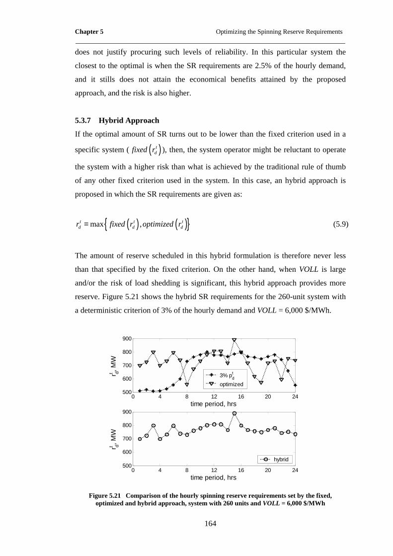
Chapter 5 Optimizing the Spinning Reserve Requirements ____________________________________________________________________
164
does not justify procuring such levels of reliability. In this particular system the
closest to the optimal is when the SR requirements are 2.5% of the hourly demand,
and it stills does not attain the economical benefits attained by the proposed
approach, and the risk is also higher.
5.3.7 Hybrid Approach
If the optimal amount of SR turns out to be lower than the fixed criterion used in a
specific system ( ( )tdfixed r ), then, the system operator might be reluctant to operate
the system with a higher risk than what is achieved by the traditional rule of thumb
of any other fixed criterion used in the system. In this case, an hybrid approach is
proposed in which the SR requirements are given as:
( ) ( ){ }max ,t t td d dr fixed r optimized r= (5.9)
The amount of reserve scheduled in this hybrid formulation is therefore never less
than that specified by the fixed criterion. On the other hand, when VOLL is large
and/or the risk of load shedding is significant, this hybrid approach provides more
reserve. Figure 5.21 shows the hybrid SR requirements for the 260-unit system with
a deterministic criterion of 3% of the hourly demand and VOLL = 6,000 $/MWh.
0 4 8 12 16 20 24500
600
700
800
900
time period, hrs
r dt , MW
0 4 8 12 16 20 24500
600
700
800
900
time period, hrs
r dt , MW
3% pdt
optimized
hybrid
Figure 5.21 Comparison of the hourly spinning reserve requirements set by the fixed, optimized and hybrid approach, system with 260 units and VOLL = 6,000 $/MWh

Chapter 5 Optimizing the Spinning Reserve Requirements ____________________________________________________________________
165
By using the hybrid approach, a reduction in the EENS cost is still obtained and thus
the overall cost of the resulting scheduling is lower, Table 5.4.
Table 5.4 Itemized costs for different fixed criteria in the 260-unit system with a VOLL = 6,000 $/MWh
Reserve
criterion
Start-up
cost (k$)
Production
cost (k$)
EENS cost
(k$)
Total cost
(k$)
Optimized 32.181 7,070.426 0.897 7,103.505
3% ptd 35.822 7,072.440 1.026 7,109.288
Hybrid 33.165 7,072.388 0.418 7,105.971
Table 5.4 shows that by using the hybrid approach the overall cost is lower than for
the fixed deterministic approach; however it is higher than the optimized approach.
This is because at some periods the hybrid approach schedules larger amounts of SR
than those determined by the auxiliary optimization process but the SR procured is
never lower than the fixed criterion.
By using the hybrid approach, the LOLP is never larger than the one attained using
the fixed criterion; however, in the periods in which the optimal SR requirements are
larger than those obtained using the fixed criterion, the associated LOLP is lower,
Figure 5.22.
0 4 8 12 16 20 240
1
2
3
4x 10⁻⁴
time period, hrs
LOLP
3% pdt
hybrid
Figure 5.22 LOLP achieved at each scheduling period with the fixed criterion and the hybrid approach for the 260-unit system and a VOLL = 6,000 $/MWh

Chapter 5 Optimizing the Spinning Reserve Requirements ____________________________________________________________________
166
5.3.8 Computation Time
The core program is in MATLAB® (MathWorks, 2005), and all the optimizations are
computed using XpressMP, (Dash Associates, 2005). The data transfer among
programs is through external files using the operating system (Windows XP).
Additionally to the UC solution process, the proposed approach requires to compute
the optimal SR requirements. The time demanded for computing these requirements
is a function of the COPT resolution, the system size and type, VOLL, maximum
MIP gap allowed, initial SR span for the search (initial upper and lower bounds) and
desired uncertainty interval. All simulations were performed in a PC with an AMD
athlon™ processor of 1.53 GHz and with 512 MB of RAM. Figure 5.23 shows the
time required to perform each of the tasks required by the algorithm and the total
computing time. In was assumed a VOLL = 6,000 $/MWh, a lower and upper bound
of 100 and 1000 MW respectively, a maximum uncertainty interval of 0.5 MW and a
COPT resolution of up to probabilities of 1×10-13 and 1 MW resolution.
26 78 130 208 2600
5
10
15
time,
min
Units
auxiliary optimizationUC calculationtotal
Figure 5.23 Computation time as a function of the system size
Figure 5.23 shows that the proposed technique is not time consuming; however the
computation times can be reduced by selecting appropriate initial lower and upper
bounds, and by relaxing the COPT resolution and/or the uncertainty length.
5.4 CONCLUSIONS
This Chapter presents a new technique to determine the SR requirements at each
period of the optimization horizon. This technique determines the amount of SR that
minimizes the total cost of operating the system, i.e. the sum of the actual operating

Chapter 5 Optimizing the Spinning Reserve Requirements ____________________________________________________________________
167
cost and of the socio-economic cost associated with load shedding. The computing
requirements associated with the proposed technique are modest compared with
those associated with other techniques that have been proposed to optimize the
amount of spinning reserve. In addition, this technique does not require the
specification of proxy measurements of risks that inevitably lead to suboptimal
solutions. Furthermore, this technique does not require a reformulation of the unit
commitment problem. It could therefore be combined with existing computer
programs. If a system operator is reluctant to require less SR than is specified by
some other criterion, a hybrid approach can be used where the SR requirement
obtained using the proposed optimization technique is only used when it is higher
than the amount specified by another criterion. This would be the case in systems
where value of lost load is high or the probability of generator outages is high.

Chapter 6 Economic Impact Assessment of LF Errors Considering the Cost of Interruptions ____________________________________________________________________
168
Chapter 6
Economic Impact Assessment of Load Forecast
Errors Considering the Cost of Interruptions
6.1 INTRODUCTION
Load forecasting plays an important role in the scheduling and security functions of
a power system. Due to the nature of the load and the numerous factors affecting it, a
prediction of its magnitude with a 100% of accuracy is not possible. However
different forecasting techniques that produce an acceptable level of accuracy can be
found in the open literature, (Gross and Galiana, 1987, Bunn, 2000). The load
information obtained by these LF techniques is used in the hydro scheduling, Unit
Commitment (UC) and hydro-thermal coordination for an economical and secure
assignation of the generating units. Inaccuracies in load prediction cause an increase
in the cost of operating the power system and on the risk measured in terms of
expectation of energy not served due to unit outages.
Unit commitment procures a given amount of spare capacity to protect the system
against contingencies and load variations. When the demand at a given period of the
optimization horizon is under-forecasted, the amount of actual spinning reserve in
the system is reduced, and thus the expected cost of unserved energy increases. On
the other hand, if the demand is over-forecasted there will be an excess of spinning
reserve that is not economically justified.
This chapter presents a comprehensive assessment of the daily economic impact of
the LF errors on the operation of the power system. The next section summarizes the
most relevant work done in this area.
Chapter 6 Economic Impact Assessment of LF Errors Considering the Cost of Interruptions ____________________________________________________________________
169
6.2 REVIEW OF PREVIOUS WORK
In (Zhai et al., 1994) a Gauss-Markov load model is used to demonstrate the effect of
the LF errors on the UC probability risk evaluation (i.e. the probability of having
insufficient committed capacity to compensate for unit failures and/or unanticipated
load variation). However, the probability of risk only measures the probability of
not being able to meet the demand under contingencies, but it does not measure the
extent in terms of load not served or a more tangible measure of the risk. This work,
therefore does not measure the economic impact of the LF errors on the system
operation.
In (Ranaweera et al., 1997) an economic impact analysis of the LF is conducted. In
this work, statistical data obtained using Monte Carlo simulations is presented to
demonstrate the effect that the LF errors have on the annual operation of the system.
In this work, the forecast errors were randomly distributed and are independent from
hour to hour.
In (Hobbs et al., 1999), the study is based on actual distributions of the forecast
errors obtained from data of two utilities. These authors also considered a wider
range of conditions. Thus, their data analysis accounts for real system conditions.
In (Teisberg et al., (forthcoming)) an assessment of the monetary savings from
reductions in LF errors due to weather forecasts improvements is conducted.
However, in none of these works is considered the effect of having a shortage of
spinning reserve due the LF errors, and thus, the societal cost of expected energy not
served is neglected.
The methodology presented in this chapter is similar to the one used in (Ranaweera
et al., 1997) and (Hobbs et al., 1999), but in this work the economic impact of the
Spinning Reserve (SR) provision is considered. The next section identifies each of
the power system costs that are affected by the LF errors.

Chapter 6 Economic Impact Assessment of LF Errors Considering the Cost of Interruptions ____________________________________________________________________
170
6.3 IDENTIFICATION OF THE COSTS
On the one hand, under-forecasting the system demand results in an insufficient
capacity to meet the SR requirements ( dr ), Figure 6.1.a. This insufficient SR
increases the probability that the synchronized capacity will not be able to meet the
demand in the case of generating unit outages. On the other hand, if the load is over-
forecasted, there will be an excess of SR and probably unnecessary start-ups of
peaking and cycling units, which reduce the overall economic efficiency, Figure
6.1.b.
(MW)
t, hrs
Committedcapacity
Spinningreserverd
pd
LF
(MW)
t, hrs
Committedcapacity
Spinningreserve
rd
LFpd
(MW)
t, hrs
Committedcapacity
Spinningreserverd
pd
LF
(MW)
t, hrs
Committedcapacity
Spinningreserverd
pd
LF
(MW)
t, hrs
Committedcapacity
Spinningreserve
rd
LFpd
(MW)
t, hrs
Committedcapacity
Spinningreserve
rd
LFpd
a) Under-forecast b) Over-forecast
Figure 6.1 Load forecast and spinning reserve
Two parts compose the overall cost of operating a power system for a given
schedule. The first is paid directly by the system operator, and consist of the sum of
the start-up and the running costs of all generating units. The second is associated
with the cases that would require shedding load in response to generation outages.
This cost is measured in terms of the impact that it has on the end users, and unlike
the cost of running the system, it is a socio-economic cost incurred by the consumers
of electrical energy. Thus this cost is a function of the energy not served and the
value that the end users attach to such energy.

Chapter 6 Economic Impact Assessment of LF Errors Considering the Cost of Interruptions ____________________________________________________________________
171
Calculating a priori the cost of an interruption is difficult because it depends on its
location, duration and the value that the different customers attach to the energy not
served, (Sullivan et al., 1996, Bell et al., 1999, Lawton et al., 2003). Thus only an
approximate value can be estimated based on historical and surveyed data. The
expected cost of an interruption or expected energy not served is considered as
explained in Chapter 2, section 2.4.
In this study the effect of the transmission and distribution networks are not taken
into account. It is also assumed that the disturbances do not extend beyond the
scheduling period during which they occur. The probability of failing to synchronize
of peaking and cycling units is not considered.
6.4 SPINNING RESERVE, RE-DISPATCH AND LOAD FORECAST
ERRORS
The SR is required to protect the system against unforeseen events such as sudden
demand increases and/or generators or tie lines outages. SR allocation (over time,
and across the generating units) has an important bearing on the dispatch and unit
commitment decision, because it comes at some cost, which ideally should be kept
minimal. This can be achieved by adjusting the SR on various generating units to
keep the total start-up/back-down and operating cost impacts at a minimum. That is
the reason why SR allocation forms part of the standard economic dispatch and unit
commitment optimization procedures.
As the system-wide SR requirement increases, the dispatch cost of the generating
units increase, because the units are not dispatched in the most economical fashion.
This cost continues increasing until a point in which more expensive generation
requires to be committed in order to fulfil the SR requirements. At the same time, as
the SR requirement increases, the cost of expected energy not served due to
generating units outages decreases, because the units will be more lightly loaded and,

Chapter 6 Economic Impact Assessment of LF Errors Considering the Cost of Interruptions ____________________________________________________________________
172
in the event of an outage, the generation of the faulted unit can be picked up by the
remaining online generation.
In Chapter 1 it was explained that the required SR is usually set on the basis of
standards developed off-line to achieve an acceptable level of risk, and some
references were introduced. Thus, if the SR requirements are not met due to an
underestimation of the load, then, the system risk will increase and this will result in
an increase in the expected cost of outages. On the other hand, if the load is
overestimated then the system operator pays the cost of carrying excess of SR and of
not operating optimally.
To illustrate these costs, the one-area IEEE-RTS system without the hydro
generation is be used as an example, Appendix B. The hydro generation is omitted
for the sake of simplicity. A VOLL of 6,000 $/MWh is assumed. Suppose that the
system forecasted and actual demand are as shown in Figure 6.2.
0 4 8 12 16 20 241500
2000
2500
3000
p d, MW
time period, hrs
0 4 8 12 16 20 24
300
350
400
SR, M
W
time period, hrs
ActualForecasted
RequiredActual
Figure 6.2 Actual and forecasted demand and required and actual SR provision
The lower part of Figure 6.2 shows the SR provided in the system. The SR is the
sum of the spare capacity of each synchronized generator ( tir ) after a re-dispatch to
meet the actual load:

Chapter 6 Economic Impact Assessment of LF Errors Considering the Cost of Interruptions ____________________________________________________________________
173
( ) ( ){ }max upmin ,t ti i i ir P p Rτ= − (6.1)
Figure 6.3 shows the increment in the dispatch cost and EENS cost due to the re-
dispatching in order to meet the actual system demand.
0 4 8 12 16 20 24-800
-600
-400
-200
0
200
time period, hrs
disp
. cos
t inr
emen
t, $
0 4 8 12 16 20 24-500
0
500
1000
1500
2000
EEN
S c
ost i
nrem
ent,
$
time period, hrs
Figure 6.3 Dispatch and EENS cost increments due to re-dispatching
Figure 6.3 shows that, in the early periods, the committed capacity in the UC
solution is insufficient to meet the actual demand and the SR requirements.
Therefore the system has to be re-dispatched to meet the load and as much of the SR
requirements as possible. By reducing the SR provision savings in the dispatch cost
are obtained. On the other hand, the cost of the EENS increases significantly. This is
because the generating units are more heavily loaded and thus the probability of
having to shed load in case of an outage increases.
In the periods where the load is overestimated, the dispatch cost increases. This is
because more generation is committed than is required. This excess generation has a
larger marginal cost. Even when this committed generation is dispatched in the most
economical fashion there could remain spare capacity. This results in an excess of
SR, and also reduces the EENS cost; however the small reduction in the EENS cost
does not compensate for the increase in the dispatch cost.

Chapter 6 Economic Impact Assessment of LF Errors Considering the Cost of Interruptions ____________________________________________________________________
174
Because the forecast error has a random behaviour, Monte Carlo simulations are
required to analyze the impact of this error. The obtained results will be subject to
statistical fluctuations, thus, any estimate of daily economic impact will not be exact,
but will have an associated error band. The next section describes a methodology for
the estimation of the daily economic impact of the load forecast error on power
system operation.
6.5 ECONOMIC IMPACT CALCULATION
Monte Carlo simulations are used to compute the daily economic impact. Monte
Carlo simulations are useful to obtain probabilistic information on a system when
some of the variables are random. In this case, the random variables are the
forecasted load. The system performance is the overall cost of the UC (i.e. start-up
cost, dispatch cost and EENS cost). Figure 6.4 shows the flowchart of the algorithm
used to compute the daily economic impact of the LF error.
6.5.1 Gather Information of the Power System In this block pertinent data for the UC computation is gathered. (i.e. generating unit
production costs, minimum and maximum generation limits, minimum up and down
times, ramp-up and –down limits). The availability of the generating units is also
collected to be used in the EENS cost calculation.
6.5.2 Compute the UC for the Actual Load In this block the optimal scheduling of the generating units for the actual load is
computed, (Wood and Wollenberg, 1996). The UC formulation includes all the
traditional constraints. In particular the spinning reserve must be greater or equal
than the capacity of the largest online generator.
This schedule is then used as a reference in order to measure the difference between
operation with a 100% accurate forecast and schedule, and the re-dispatch of the
committed generators to meet the actual load.

Chapter 6 Economic Impact Assessment of LF Errors Considering the Cost of Interruptions ____________________________________________________________________
175
Gather Information of the Power System
Simulate LoadForecasting
Run UC for theForecasted Load
Re-Schedule to Meet the Actual Load
Operating CostsCalculation
Meet MC Criterion?
Compute the Economic Impact
noyes
ComputeUC for the Actual Load
.
Operating CostsCalculation
end
Gather Information of the Power System
Simulate LoadForecasting
Run UC for theForecasted Load
Re-Schedule to Meet the Actual Load
Operating CostsCalculation
Meet MC Criterion?
Compute the Economic Impact
noyes
ComputeUC for the Actual Load
.
Operating CostsCalculation
end
Figure 6.4 Flow chart of the algorithm to compute the economical impact of the LF error
6.5.3 Operating Costs Calculation The operating cost is calculated as the sum of the start-up cost, the production costs
of the generating units and the EENS cost. A quadratic approximation of the
production cost is used, thus the production cost at period t is given as:
( ) ( )2t t t ti i i i i i ic p a p b p c= + + (6.2)
Where ( )t ti ic p is the cost of producing t
ip MW with unit i at period t . The
parameters ia , ib and ic were taken from (Wang and Shahidehpour, 1993); refer to
Appendix B for further details.
In this block the EENS is also calculated at each period of the optimization horizon
and weighted by the VOLL to obtain the EENS cost.

Chapter 6 Economic Impact Assessment of LF Errors Considering the Cost of Interruptions ____________________________________________________________________
176
6.5.4 Simulate Load Forecasting This block simulates the forecasting of the load. At each hour, the forecasted load is
equal to the actual load plus an error term:
t t t
dLF p error= + (6.3)
Where tLF is the system load forecast at period t , tdp is the system wide demand at
period t and terror is the error due to the forecast at period t . The error is generated
from a Gaussian distribution (Papoulis and Pillai, 2002) with a zero mean, and a
standard deviation equal to a percentage of the actual load. In this study the standard
deviation is assumed to be 1, 3 and 5%. The error at the first period is produced by
means of using a uniform random number generator and using the cumulative
probability distribution of the error. The random number at the second period will be
within a predefined window in order to introduce coherence and correlation among
errors. This process is illustrated in Figure 6.5.
-400 -200 0 200 4000
0.2
0.4
0.6
0.8
1
Error, MW
prob
abilit
y
period t
-400 -200 0 200 4000
0.2
0.4
0.6
0.8
1
Error, MW
prob
abilit
y
period t+1
wt wt+1
rnt rnt+1
Figure 6.5 Load forecast error for a demand at t of 2200 MW and a demand at 1t + of 2000 MW, both with 5%σ = of the demand
Figure 6.5 shows the cumulative distribution of the errors for a load of 2200 MW at
period t and 2200 MW at period 1t + both with 5%σ = of the load at such period.
At period t a random number is generated (rnt); then a window (wt) is also generated
and the random number at period 1t + (rnt+1) cannot lie outside of wt. The width of
this window is predefined. Once the random number at period 1t + has been
generated a new window is created (wt+1) and the random number at period 2t +
Chapter 6 Economic Impact Assessment of LF Errors Considering the Cost of Interruptions ____________________________________________________________________
177
cannot lie outside of this window. This process is repeated over the whole
optimization horizon.
6.5.5 Run UC for the Forecasted Load The UC is calculated for the forecasted load. By doing so a schedule is obtained in
which the erroneous load and SR requirements are satisfied.
6.5.6 Re-Schedule to Meet the Actual Demand The schedule obtained for the forecasted load is not the optimal solution to meet the
actual demand. Therefore the committed units must be re-dispatched. A dynamic
economic dispatch can be applied if the SR requirements are considered, (Han et al.,
2001). However, this might lead to infeasible solutions if the SR cannot be met with
the already synchronized units.
Since one of the main functions of the SR is to provide spare capacity to avert load
disconnection in the case of sudden generating outages or load increases, then when
the forecast underestimates the actual load, the SR provision at such period will not
be as large as the one originally scheduled since part of it is being used. During the
re-dispatch the following constraint for the SR requirements is enforced at all periods
of the optimization horizon:
( ) ( ) ( )( )max maxmin max ,maxt t t t td i i i i di i
r u P u P LF p≥ + − (6.4)
It is also possible that the dispatch of the synchronized units does not produce a
feasible solution for the actual load due to ramp-up or ramp–down limitations of the
generating units at different periods of the optimization horizon; and at the same
time meeting a minimum level of spinning reserve. To overcome this problem it is
allowed to commit extra generation while keeping the previously committed units.
Thus this block tries to mimic the decisions taken by a system operator at the
moment of meeting the actual demand. To do so, in the UC formulation the
following constraint is enforced for all generating units and at all periods of the
optimization horizon:

Chapter 6 Economic Impact Assessment of LF Errors Considering the Cost of Interruptions ____________________________________________________________________
178
t ti iu δ≥ (6.5)
Where [ ], 0,1t ti iu δ ∈ ; and t
iδ is the schedule obtained for the forecasted load. That
is, this re-schedule allows only the commitment of extra units just to fulfil the system
requirements and avert infeasibility. Interconnections with other power systems are
not considered.
6.5.7 Compute the Economic Impact In this block the difference between the re-scheduling cost and the cost of the
scheduling for the load with no error is computed. This data is also stored to be used
to compute the Monte Carlo criterion of convergence.
6.5.8 Meet the Monte Carlo Convergence Criterion At this stage of the algorithm all the data simulated is used to compute the Monte
Carlo criterion of convergence. Different criteria to determine whether the Monte
Carlo criterion has been satisfied or not can be applied. In (Hahn and Shapiro, 1967)
an approximate way to find the required number of samples is given as:
2
1 2'z
nEα σ
− =
(6.6)
Where:
E : maximum allowable error in estimating the economic impact
1 α− : desired probability or confidence level that the true economic impact does
not differ from estimated economic impact by more than E±
'σ : initial estimate of standard deviation of cost impact
1 2
z α−: ( )1 1002
α− percent point of a standard normal distribution

Chapter 6 Economic Impact Assessment of LF Errors Considering the Cost of Interruptions ____________________________________________________________________
179
The values of E and 'σ cannot be guessed arbitrarily, thus it is suggested to first
make an initial Monte Carlo simulation to get an estimate of the final values of the
error and the standard deviation.
Some other criteria for convergence can also be applied. For instance a criterion in
which the Monte Carlo simulation will be stopped after EI
σκ = has reached a
predefined value or it does not undergo a significant change after a given number of
samples can also be enforced, (Billinton and Li, 1994). σ is the standard deviation
of the economic impact; EI is the economic impact and EI is the economic
impact’s mean.
In this study both criteria were enforced. Equation (6.6) was used to determine a
minimum number of samples. If after this criterion has been satisfied the standard
deviation continues changing then the simulation continues.
6.6 TEST RESULTS
The proposed economic impact assessment formulation was tested on the IEEE-RTS
single area system without hydro generation, (Grigg et al., 1999). The UC program
and the re-dispatch program were implemented in XpressMP (Dash Associates,
2005), and a MIP gap no larger than 0.07% was considered adequate. The system
data is the same as used in section 6.4. The load profile used as the actual load was
taken from (Wang and Shahidehpour, 1993), more details of the system and load
profile can be found in Appendix B.
6.6.1 Effect of the Load Forecast Accuracy The accuracy of the forecast can be adjusted by changing the standard deviation of
the Gaussian error. Three values of the standard deviation were considered: 1, 3 and
5 % of the actual load in a given period. Monte Carlo trials were performed until
1000 simulations have been performed or κ become less than 0.0027, 0.0012 and
0.0004 respectively (the value of κ changes because the standard deviation of the

Chapter 6 Economic Impact Assessment of LF Errors Considering the Cost of Interruptions ____________________________________________________________________
180
economic impact decreases with the forecast error). In this simulation the inter-
temporal window is considered to be 0.5 and is centred.
The UC for the load with no error gives the following costs: Start-up cost: $
4,471.00, dispatch cost: $ 736,175.55 and EENS cost: $ 590.05; that is an overall
cost of $ 741,236.61 with an average cost of energy of 13.493 $/MWh. Table 6.1
shows the results of the Monte Carlo simulation.
Table 6.1 Daily economic impact
Forecast Error
(σLF), %
EI’s mean
( EI ), $
EI’s standard
deviation (σ), $
1 590.14 274.25
3 1,651.70 891.67
5 3,293.50 1,948.90
Figure 6.6 shows the cumulative distribution for the daily impact for the different
forecast errors. From this figure it can be appreciated that the economic impact
decreases as the forecast error decreases. For instance, by improving the forecast
from 5 to 1% savings of around 0.36% can be achieved in the operation of the
system.
0 1000 2000 3000 4000 5000 6000 7000 8000 9000 100000
0.1
0.2
0.3
0.4
0.5
0.6
0.7
0.8
0.9
1
Economic Impact, $
Pro
babi
lity
LF = 5% LF = 3% LF = 1%
σ σ σ
Figure 6.6 Cumulative distribution of the daily economic impact for different load forecast errors
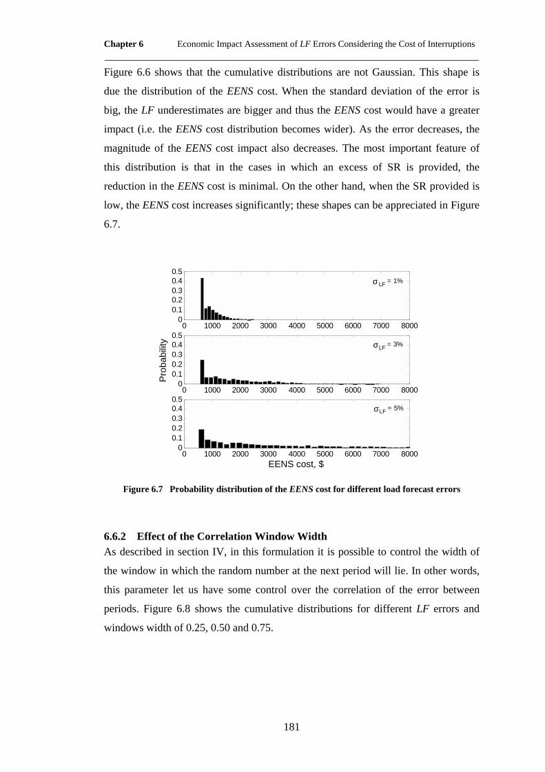
Chapter 6 Economic Impact Assessment of LF Errors Considering the Cost of Interruptions ____________________________________________________________________
181
Figure 6.6 shows that the cumulative distributions are not Gaussian. This shape is
due the distribution of the EENS cost. When the standard deviation of the error is
big, the LF underestimates are bigger and thus the EENS cost would have a greater
impact (i.e. the EENS cost distribution becomes wider). As the error decreases, the
magnitude of the EENS cost impact also decreases. The most important feature of
this distribution is that in the cases in which an excess of SR is provided, the
reduction in the EENS cost is minimal. On the other hand, when the SR provided is
low, the EENS cost increases significantly; these shapes can be appreciated in Figure
6.7.
0 1000 2000 3000 4000 5000 6000 7000 80000
0.10.20.30.40.5
0 1000 2000 3000 4000 5000 6000 7000 80000
0.10.20.30.40.5
Prob
abilit
y
0 1000 2000 3000 4000 5000 6000 7000 80000
0.10.20.30.40.5
EENS cost, $
LF = 1%
LF = 3%
LF = 5%
σ
σ
σ
Figure 6.7 Probability distribution of the EENS cost for different load forecast errors
6.6.2 Effect of the Correlation Window Width As described in section IV, in this formulation it is possible to control the width of
the window in which the random number at the next period will lie. In other words,
this parameter let us have some control over the correlation of the error between
periods. Figure 6.8 shows the cumulative distributions for different LF errors and
windows width of 0.25, 0.50 and 0.75.
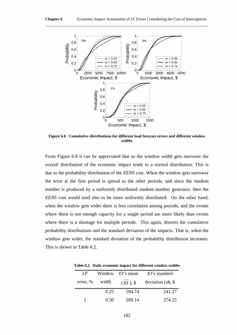
Chapter 6 Economic Impact Assessment of LF Errors Considering the Cost of Interruptions ____________________________________________________________________
182
0 2500 5000 7500 100000
0.2
0.4
0.6
0.8
1
Economic Impact, $
Pro
babi
lity
0 1500 3000 4500 60000
0.2
0.4
0.6
0.8
1
Economic Impact, $
Pro
babi
lity
0 500 1000 15000
0.2
0.4
0.6
0.8
1
Economic Impact, $
Pro
babi
lity
w = 0.25w = 0.50w = 0.75
w = 0.25w = 0.50w = 0.75
w = 0.25w = 0.50w = 0.75
5% 3%
1%
Figure 6.8 Cumulative distributions for different load forecast errors and different window widths
From Figure 6.8 it can be appreciated that as the window width gets narrower the
overall distribution of the economic impact tends to a normal distribution. This is
due to the probability distribution of the EENS cost. When the window gets narrower
the error at the first period is spread to the other periods, and since the random
number is produced by a uniformly distributed random number generator, then the
EENS cost would tend also to be more uniformly distributed. On the other hand,
when the window gets wider there is less correlation among periods, and the events
where there is not enough capacity for a single period are more likely than events
where there is a shortage for multiple periods. This again, distorts the cumulative
probability distributions and the standard deviation of the impacts. That is, when the
window gets wider, the standard deviation of the probability distribution increases.
This is shown in Table 6.2.
Table 6.2 Daily economic impact for different window widths
LF
error, %
Window
width
EI’s mean
( EI ), $
EI’s standard
deviation (σ), $
0.25 594.74 241.27
1 0.50 590.14 274.25

Chapter 6 Economic Impact Assessment of LF Errors Considering the Cost of Interruptions ____________________________________________________________________
183
0.75 612.05 339.29
0.25 1,708.8 814.75
3 0.50 1,651.7 891.67
0.75 1,780.6 1,291.30
0.25 3,239.4 1,497.90
5 0.50 3,293.5 1,948.90
0.75 3,762.5 2,816.00
Figure 6.9 shows the probability distributions of the EENS cost for the case of 5%
error and with three different window widths. As expected, when the correlation
between periods increases, the EENS cost is more uniformly distributed. When the
correlation is reduced, there are more cases where the impact is close to the
minimum, but there are still cases in which the EENS cost impact is large.
0 2000 4000 6000 8000 100000
0.10.20.30.40.5
0 2000 4000 6000 8000 100000
0.10.20.30.40.5
Prob
abilit
y
0 2000 4000 6000 8000 100000
0.10.20.30.40.5
EENS cost, $
w = 0.25
w = 0.50
w = 0.75
Figure 6.9 Probability distribution for a forecast error of 5% with different window width
Table 6.3 shows the daily economic impact as a percentage of the total operating
cost for a perfect load forecast. These values are computed using the mean values of
the economic impact. For all window widths the economic impact increases with the
error in the LF. Significant savings can thus be achieved by LF refinements.
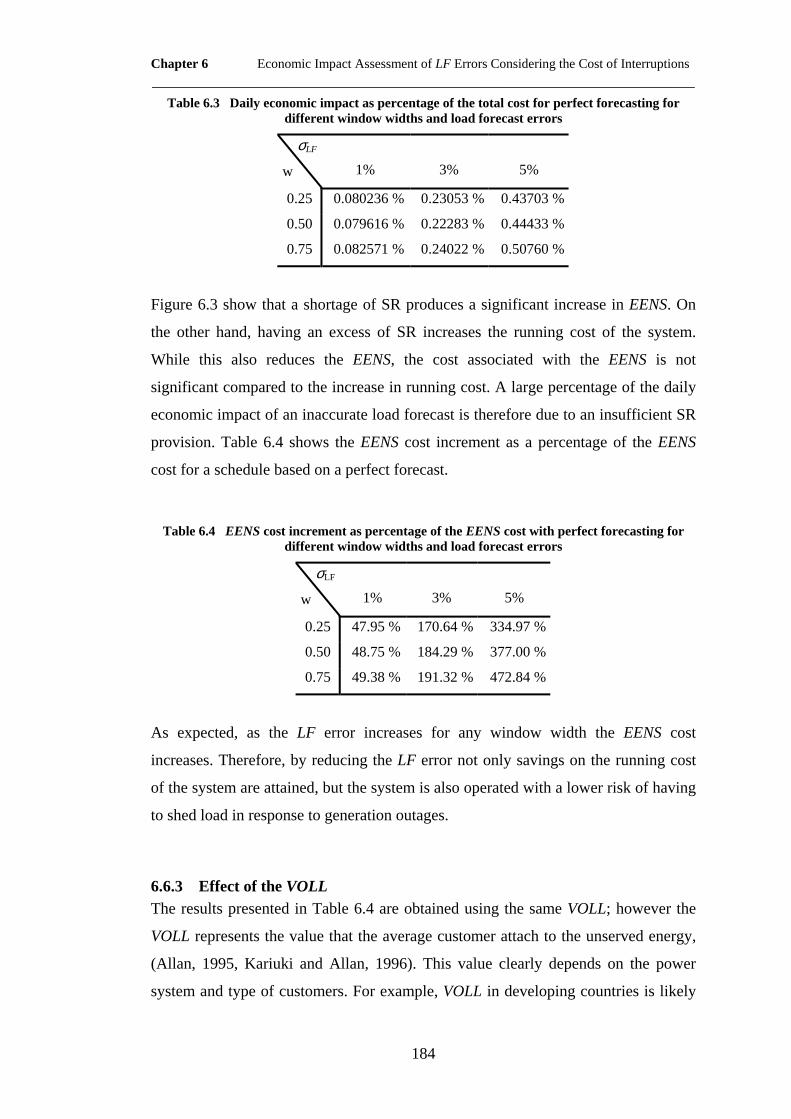
Chapter 6 Economic Impact Assessment of LF Errors Considering the Cost of Interruptions ____________________________________________________________________
184
Table 6.3 Daily economic impact as percentage of the total cost for perfect forecasting for different window widths and load forecast errors
σLF
w
1%
3%
5%
0.25 0.080236 % 0.23053 % 0.43703 %
0.50 0.079616 % 0.22283 % 0.44433 %
0.75 0.082571 % 0.24022 % 0.50760 %
Figure 6.3 show that a shortage of SR produces a significant increase in EENS. On
the other hand, having an excess of SR increases the running cost of the system.
While this also reduces the EENS, the cost associated with the EENS is not
significant compared to the increase in running cost. A large percentage of the daily
economic impact of an inaccurate load forecast is therefore due to an insufficient SR
provision. Table 6.4 shows the EENS cost increment as a percentage of the EENS
cost for a schedule based on a perfect forecast.
Table 6.4 EENS cost increment as percentage of the EENS cost with perfect forecasting for different window widths and load forecast errors
σLF
w
1%
3%
5%
0.25 47.95 % 170.64 % 334.97 %
0.50 48.75 % 184.29 % 377.00 %
0.75 49.38 % 191.32 % 472.84 %
As expected, as the LF error increases for any window width the EENS cost
increases. Therefore, by reducing the LF error not only savings on the running cost
of the system are attained, but the system is also operated with a lower risk of having
to shed load in response to generation outages.
6.6.3 Effect of the VOLL The results presented in Table 6.4 are obtained using the same VOLL; however the
VOLL represents the value that the average customer attach to the unserved energy,
(Allan, 1995, Kariuki and Allan, 1996). This value clearly depends on the power
system and type of customers. For example, VOLL in developing countries is likely

Chapter 6 Economic Impact Assessment of LF Errors Considering the Cost of Interruptions ____________________________________________________________________
185
to be significantly lower because the cost of interruptions is not as significant as in
countries where the economy is more dependent on a continuous supply of energy.
The accuracy of the LF thus has different impacts on different systems. Figure 6.10
shows the economic impact mean as a function of the forecast errors for different
VOLLs and window width.
1 2 3 4 50
2000
4000
6000
Forecast error, %E
cono
mic
impa
ct, $
1 2 3 4 50
2000
4000
6000
Forecast error, %
Eco
nom
ic im
pact
, $
1 2 3 4 50
2000
4000
6000
Forecast error, %
Eco
nom
ic im
pact
, $
VOLL = 2000 $/MWhVOLL = 4000 $/MWhVOLL = 6000 $/MWhVOLL = 8000 $/MWhVOLL = 10000 $/MWh
w = 0.25 w = 0.50
w = 0.75
Figure 6.10 Economic impact mean as a function of the forecast error for different VOLLs and window width
Figure 6.10 shows that as the VOLL increases the mean economic impact increases.
As the correlation among errors in the forecast decreases (larger window widths) the
economic impact increment as a function of the forecast error is “steeper”. That is,
for small reductions in the forecast accuracy, the economic and societal penalization
is larger.
As an operator responsible for the load forecast, one of the main concerns is to know
how accurate should the load forecast be. The point at which it might not worth to
invest in improving the accuracy of the forecast is such that the economic impact
does not decrease significantly as the load forecast error decreases. As shown in
Figure 6.10, this point will vary according to the VOLL. This figure also shows that
systems in which VOLL is large require higher accuracy in the forecast of the load,
Chapter 6 Economic Impact Assessment of LF Errors Considering the Cost of Interruptions ____________________________________________________________________
186
since the errors can result in shortages of capacity that can lead to load shedding,
which has a large societal penalization.
6.7 CONCLUSIONS
This chapter presented a more comprehensive economical impact assessment of the
load forecast errors on the daily operation of the power system. This assessment
includes the cost of expected energy not served due to the occasional generating
units outages. It has been shown that this cost will increase when the system does not
have enough capacity to meet both the demand and the spinning reserve
requirements.
If in the economic impact the cost of the expected energy not served is not
considered, the only impact will be associated with the re-dispatching of the online
generation and the start-up cost of the generating units required to meet the system
requirements. This assessment gives optimistic estimates since the shortage of SR is
not considered.

Chapter 7 Conclusions and Suggestions for Further Work ____________________________________________________________________
187
Chapter 7
Conclusions and Suggestions for Further Work
7.1 CONCLUSIONS
This thesis proposes and formulates a theoretical unit commitment that minimizes a
combined objective, which is the sum of the running cost of the system and the
expected cost of energy not served due to capacity deficits. This approach is
compared with the reserve constraint traditionally enforced in the dispatch and
commitments algorithms, and against an approach that commits spinning reserve
until a loss of load probability target is attained. The proposed approach
demonstrated its advantages over other approaches, and these can be listed as
follows:
• It implicitly determines the required levels of spinning reserve by explicitly
adjusting the expected cost of unserved energy due to random outages until
the cost of providing the spinning reserve no longer justifies it
• It does not require the traditional reserve constraint to set a fixed amount of
spinning reserve
• It does not require risk targets to be attained
• The proposed approach is self-contained and, as a consequence it does not
require exogenous cost/benefit analyses to compute a risk target
• By not enforcing the traditional reserve constraint infeasibilities of solution
are averted
This proposed approach includes the full expected energy not served distribution on
the unit commitment calculation. The expected energy not served distribution is
Chapter 7 Conclusions and Suggestions for Further Work ____________________________________________________________________
188
computed off-line and fed to the optimization process, and for each possible
combination of units the optimization procedure trigger the appropriate expected
energy not served value by a binary variable. This approach is useful to demonstrate
the advantages of including the extra term in the objective function to determine the
optimal levels of spinning reserve. However, due the combinatorial explosion of the
possible permutations of units, this approach is not directly applicable to power
systems of realistic size.
Clearly, in order to make the proposed technique applicable, the expected cost of the
outages must be estimated easily for any combination of generating units. While
techniques for its rigorous calculation exist, the main problem stems from the fact
that there are no direct means of incorporating these calculations within the
optimization problem or the process would require a prohibitive amount of
computing time to reach a solution. Therefore, a fast and yet accurate method for
estimating the expected energy not served for any combination of units that the unit
commitment calculation may consider has been developed. This proxy is
incorporated in the unit commitment formulation by sets of linear constraints. This
formulation showed its applicability for systems of different sizes by getting lower
overall operating costs compared with the unit commitment approaches that enforce
the spinning reserve requirements based on “rules of thumb”.
The proposed model is then extended to consider the failures to synchronize of the
generating units. This is achieved by further extending the EENS proxies to be
sensitive to an additional variable: the capacity on synchronization. It was shown
that the EENS considering the failure to synchronize of the generating units is larger
than if these failures are disregarded. Thus, it was shown that by shifting some MW
on synchronization to other periods of the optimization horizon, the overall EENS
cost of the system decreases. The proposed model was validated using Monte Carlo
methods and then included into the optimization process by sets of linear constraints.
It was shown that in principle this approach results in lower overall costs; however
the amount of variables also results into a heavier computational burden and long
computation times; this formulation also results into large MIP gaps.

Chapter 7 Conclusions and Suggestions for Further Work ____________________________________________________________________
189
An offline approach to optimize the spinning reserve requirements at each period of
the optimization horizon prior the unit commitment calculation was also presented.
In this approach, the optimal spinning reserve requirements are obtained by making a
balance between its cost of provision and the benefit derived from this reserve
measured in terms of EENS cost reduction for a given value of lost load. Therefore
these spinning reserve requirements minimize the sum of reserve cost and expected
cost of outages. The proposed approach is tested in systems of different sizes. In
each case, the proposed approach results in a lower overall cost and a more
homogeneous risk distribution among the periods of the optimization horizon. A
hybrid approach is also proposed to deal with the cases where the optimal spinning
reserve requirements turn out to be lower than those obtained using the fixed
criterion. In this hybrid approach the spinning reserve requirements are determined
by the maximum between the fixed criterion and the optimized approach; thus, the
operating “risk” of the system is never lower than the one that would be attained
using the fixed criterion. On the other hand, in the cases where the expected cost of
outages is large, or for systems where the value of lost load is large, this approach
schedules larger amounts of spinning reserve and thus reduces the overall operating
cost of the system. The hourly LOLP is also lower or equal to the one obtained using
the traditional rule-of-thumb.
An assessment of the load forecast error on the daily operation of the power system
is carried out. This assessment is comprehensive since it includes the expected cost
of outages. It was shown that the expected cost of outages is sensitive to the spinning
reserve provision, thus when the provision is lower than the predefined amount, the
expected cost of outages increases significantly. On the other hand, when the
spinning reserve provision is larger than the scheduled amount due to load forecast
errors, the reduction in the expected cost of outages does not compensate for the
associated increment in the running cost of the system. Thus, this term must be used
to assess the impact of the load forecast. In this section, it is also shown that the
answer to the question: “How accurate should the load forecast process should be?”
is highly dependent on the system’s value of lost load.

Chapter 7 Conclusions and Suggestions for Further Work ____________________________________________________________________
190
7.2 Suggestions for Further Work
In this section a few ideas that might enhance the proposed models are discussed.
• In this thesis it has been proposed to consider not only the probability that the
generating units would go on outage, but also the probability that these
generating units fail to synchronize. This was proposed by a three-state
reliability model, which was validated by Monte Carlo simulations.
However, the mathematical modelling to include such model into the
optimization process is cumbersome. Thus, as a future work it is proposed to
include a discretized model of the surface that define the product of the slope
and the capacity on synchronization in order to reduce the burden of the
proposed model.
• In real power systems/markets, the spinning reserve caters for more than just
the random generator outages. In reality any part of the system might
undergo an outage limiting the ability of the remaining synchronized
generation to effectively pick-up the demand. For instance, in some
topologies the outage of transmission lines might limit the spinning reserve,
even if enough spare capacity is available. Thus, the effect of the
transmission system on the power flows and on the expected energy not
served must be considered. Ideally, the proposed approaches should be
extended to include an optimal power flow solution to achieve the overall
optima considering the transmission constraints.
• In the optimal commitments presented in this thesis it was assumed that the
load forecast was 100% accurate. In reality, this is an optimistic assumption
since in a 24 hours horizon the demand cannot be predicted with such
accuracy. In practice, the load forecast has an error associated. It was also
shown throughout the thesis that the optimal spinning reserve requirements
are clearly dependent of the demand to serve. Thus, the short-term load
forecast errors will affect the spinning reserve requirements and can either
result in low or large spinning reserve provision depending on the error.
Chapter 7 Conclusions and Suggestions for Further Work ____________________________________________________________________
191
Therefore including the load forecast errors enhances the model and results in
a more realistic risk estimation.
• In power systems across the world the penetration of intermittent generation
sources is increasing in order to attain reductions in CO2 emissions. Since
these intermittent generating sources (e.g. wind power generation and solar
panels among others) cannot be scheduled and dispatched in the classical
way because of their intrinsic dependence on varying weather conditions new
models are required. The integration of these sources affects not only the unit
commitment and dispatch, but also has a clear impact on the reliability and
spinning reserve requirements. This is because this alternative generation is
designed to maximize the extraction of energy from the renewable sources
(i.e. wind, sun, etc) rather than to respond to a grid operator’s dispatch.
Clearly, the power generation is a function of the stochastic wind or sun
availability; thus, this impacts the way in which the system is operated. The
intermittent generation can be modelled in a similar way as the load forecast
errors; and the uncertainty could also be correlated using the model presented
in Chapter 6 for the load forecast errors. These additional generations can
then be modelled as a negative load. One possible way to tackle this problem
is by using stochastic programming techniques.
• The role of the demand side participation into the market clearing process
and units commitment should also be investigated. Through the thesis it was
assumed that the demand is inelastic and that the demand does not play an
active role in the bidding process. In reality, the overall demand can be
modelled as a set of bids that have a clear impact on the resulting units
commitment, power production and spinning reserve procurement.
• The proposed approaches are applicable to power systems of any size. It is
believed that power systems might start disaggregating into smaller active
parts or cells. This is because of the increasing penetration of micro-sources
within the distribution networks. Some of these small generations will not
produce electrical energy only but also heat as in the case of combined heat
Chapter 7 Conclusions and Suggestions for Further Work ____________________________________________________________________
192
and power stations. This will introduce thermal constraints into the
optimization process due to the “must-run” character of these stations at
some periods of the optimization horizon. These thermal constraints must be
modelled and included in the optimization process.
• In the simulation results presented it was assumed that the contingencies
occur at a given period of time and that they do not extend beyond that
period. In reality this might be optimistic, and thus a more complete model
should include the multi-period effect of the contingencies.

Appendix A Failure Probabilities ____________________________________________________________________
193
Appendix A
FAILURE PROBABILITIES
A.1 GENERATING UNITS’ OUTAGE PROBABILITIES
The basic generating unit parameter used in static capacity evaluation is the
probability of finding the unit on forced outage at some time in the future. This
probability is the unit unavailability. Historically in power systems, it is known as
the Forced Outage Rate (FOR), (Billinton and Allan, 1996). This dimensionless
quantity measures the per unit time a given generating unit is out of service due to
random failures and is given by:
( ) ( )U e λ µλ λλ µ λ µ
− + ΤΤ = −+ +
Where:
λ expected failure rate (reciprocal of the mean time to failure), times/hrs
µ expected repair rate (reciprocal of the mean time to repair), times/hrs
Τ mission time, hrs
However, for operation studies purposes the mission time is defined as the time span
of the study analysis (e.g. for unit commitment studies usually half or one hour
resolution is used). In operational studies the mean time to repair is very large
compared to the mission time, thus the repair process can be neglected, i.e. 0µ = .
The unavailability of the generating unit is then given by:
1U e λ− Τ= −

Appendix A Failure Probabilities ____________________________________________________________________
194
This is known as the Outage Replacement Rate (ORR) and represents the probability
that a unit fails and is not replaced during the mission time Τ . It also should be noted
that it has been assumed that the failures are exponentially distributed.
Power systems are composed by sets of generating units, these sets together form a
generation model; and the reliability generation model used for loss of load
assessment is known as Capacity Outage Probability Table (COPT), (Billinton and
Allan, 1996). As the name suggests, it is a table that lists capacity levels and the
associated levels of probabilities of existence. If a power system is composed of a
set of generating units { }1, 2, , N= …N , in which each of the generating units has a
capacity ,nC n∀ ∈ N , and an associated relative unavailability ,nU n∀ ∈ N , then
the COPT is generated as shown in Table A.1.
Table A.1. Contingency enumerated capacity outage probability table
Number of units out
Number of combinations
Capacity on Outage (MW)
Probability of occurrence
0
1
0 ( )
1
1N
nn
U=
−∏
1 ( )
!1 !
NN −
iC ( )1
1N
i nnn i
U U=≠
−∏
2 ( )
!2! 2 !
NN −
i jC C+ i ≠ j
( )1,
1N
i j nnn i j
U U U=≠
−∏
" " " "
N 1
1
N
nn
C=∑ ( )
1
N
nn
U=
∏

Appendix B Systems Data ____________________________________________________________________
195
Appendix B
SYSTEMS DATA
B.1 26-UNIT SYSTEM
The 26-unit system used for testing is derived from the IEEE-RTS single-area
system (Grigg et al., 1999). If the hydro generating units are omitted, this system
consists of 26 units with a total generation capacity of 3105 MW. The quadratic
approximation of the cost functions and ramp-up limits were taken from (Wang and
Shahidehpour, 1993). The reason why the RTS was selected is due the fact that this
system was not developed with the intention of being a characteristics system or
typical power system. Therefore this test system is hybrid and atypical and its
characteristics are more universal. The type of generating units and their start-up cost
are shown in Table B.1.
Table B.1 Unit type and start-up cost
Group Number
of units
Unit Type Capacity
(MW)
Start-up
Cost ($)
A 5 Oil/Steam 12 68
B 4 Oil/CT 20 5
C 4 Coal/Steam 76 655.6
D 3 Oil/Steam 100 566
E 4 Coal/Steam 155 1048.3
F 3 Oil/Steam 197 775
G 1 Oil/Steam 350 4468
H 2 Nuclear 400 N/A

Appendix B Systems Data ____________________________________________________________________
196
The mean time to failure (MTTF) outage remplacement rate (ORR), probability of
failing to synchronize (Ps) and overall probably of failing (Pf) are shown in Table
B.2.
Table B.2 Generating units’ reliability data
Group Number
of units
MTTF
(hrs)
ORR Ps Pf
A 5 2940 0.00034 0.0148 0.015135
B 4 450 0.002222 0.0201 0.022275
C 4 1960 0.00051 0.044 0.044488
D 3 1200 0.000833 0.0399 0.0407
E 4 960 0.001041 0.0291 0.030111
F 3 950 0.001052 0.025 0.026026
G 1 1150 0.000869 0.001 0.001868
H 2 1100 0.000909 0.000 0.000909
Table B.3 shows the minimum and maximum stable generations and coefficients of
the quadratic approximation of the cost functions of each of the generating units.
Table B.3 Generating units’ production limits and coefficients of the quadratic cost function
Group Unit
Pmin
(MW)
Pmax
(MW)
ai
($/MW2h)
bi
($/MWh)
ci
($/h)
1 2.4 12.0 0.02533 25.5472 24.3891
2 2.4 12.0 0.02649 25.6753 24.4110
3 2.4 12.0 0.02801 25.8027 24.6382
4 2.4 12.0 0.02842 25.9318 24.7605
A
5 2.4 12.0 0.02855 26.0611 24.8882
6 4.0 20.0 0.01199 37.5510 117.7551
7 4.0 20.0 0.01261 37.6637 118.1083
8 4.0 20.0 0.01359 37.7770 118.4576
B
9 4.0 20.0 0.01433 37.8896 118.8206
10 15.2 76.0 0.00876 13.3272 81.1364
11 15.2 76.0 0.00895 13.3538 81.2980
C
12 15.2 76.0 0.00910 13.3805 81.4641

Appendix B Systems Data ____________________________________________________________________
197
13 15.2 76.0 0.00932 13.4073 81.6259
14 25.0 100.0 0.00623 18.0000 217.8952
15 25.0 100.0 0.00612 18.1000 218.3350
D
16 25.0 100.0 0.00598 18.2000 218.7752
17 54.24 155.0 0.00463 10.694 142.7348
18 54.24 155.0 0.00473 10.7154 143.0288
19 54.24 155.0 0.00481 10.7367 143.3179
E
20 54.24 155.0 0.00487 10.7583 143.5972
21 68.95 197.0 0.00259 23.0000 259.1310
22 68.95 197.0 0.00260 23.1000 259.6490
F
23 68.95 197.0 0.00263 23.2000 260.1760
G 24 140.0 350.0 0.00153 10.8616 177.0575
25 100.0 400.0 0.00194 7.4921 310.0021 H
26 100.0 400.0 0.00195 7.5031 311.9120
0 50 100 150 200 250 300 350 4000
500
1000
1500
2000
2500
3000
3500
4000
4500
5000
production, MW
cost
, $/h
r
Group A
Group B
Group C
Group D Group E
Group G Group F
Group H
Figure B.1 Production costs of the generating units as a function of the power produced
Table B.4 shows the generating unit’s minimum up-times and down-times as well as
the maximum ramp-up and ramp-down limits. While in (Grigg et al., 1999) ramp
rates for the generating units, the ones in (Wang and Shahidehpour, 1993) were
preferred because, the lasts are lower and thus limit the generating unit’s spare
capacity. This has a direct effect on the expected energy not served.

Appendix B Systems Data ____________________________________________________________________
198
Table B.4 Generating units’ minimum up- and down-times and maximum ramp-up and -down
Group Min. up-
time, hrs
Min.
down-
time, hrs
History*
(tiH), hrs
Max.
Ramp-up,
MW/h
Max. Ramp-
down, MW/h
A 1 1 -1 48.0 60.0
B 1 1 -1 30.5 70.0
C 3 2 3 38.5 80.0
D 4 2 -3 51.0 74.0
E 5 3 5 55.0 78.0
F 5 4 -4 55.0 99.0
G 8 5 10 70.0 120.0
H 8 5 10 50.5 100.0
* The negative sign terms denotes that the unit was off during the absolute value of the history
The load profile used to test the system is given in Table B.5.
Table B.5 Load profile for the 26-unit system
hour ptd (MW) hour pt
d (MW) hour ptd (MW)
1 1700 9 2540 17 2550
2 1730 10 2600 18 2530
3 1690 11 2670 19 2500
4 1700 12 2590 20 2550
5 1750 13 2590 21 2600
6 1850 14 2550 22 2480
7 2000 15 2620 23 2200
8 2430 16 2650 24 1840
B.2 78-UNIT SYSTEM
The 78-unit system is derived from the RTS-96 system. Three RTS-79 areas
compose this system. The hydro generation has been removed. The costs of each of
the RTS-79 areas have been slightly altered in order to prevent the optimization
engine from finding equal objective function costs for different solutions. The

Appendix B Systems Data ____________________________________________________________________
199
minimum and maximum stable generation and coefficients of the quadratic
approximation are shown in Table B.6.
Table B.6 Generating units’ production limits and coefficients of the quadratic cost function
Group Unit
Pmin
(MW)
Pmax
(MW)
ai
($/MW2h)
bi
($/MWh)
ci
($/h)
1 2.4 12 0.02533 25.5472 24.3891
2 2.4 12 0.02649 25.6753 24.4110
A1 3 2.4 12 0.02801 25.8027 24.6382
4 2.4 12 0.02842 25.9318 24.7605
5 2.4 12 0.02855 26.0611 24.8882
6 2.4 12 0.02609 26.3136 25.1208
7 2.4 12 0.02728 26.4456 25.1433
A2 8 2.4 12 0.02885 26.5768 25.3773
9 2.4 12 0.02927 26.7098 25.5033
10 2.4 12 0.02941 26.8429 25.6348
11 2.4 12 0.02685 27.0800 25.8524
12 2.4 12 0.02808 27.2158 25.8757
A3 13 2.4 12 0.02969 27.3509 26.1165
14 2.4 12 0.03013 27.4877 26.2461
15 2.4 12 0.03026 27.6248 26.3815
16 4 20 0.01199 37.5510 117.7551
B1 17 4 20 0.01261 37.6637 118.1083
18 4 20 0.01359 37.7770 118.4576
19 4 20 0.01433 37.8896 118.8206
20 4 20 0.01235 38.6775 121.2878
B2 21 4 20 0.01299 38.7936 121.6515
22 4 20 0.01400 38.9103 122.0113
23 4 20 0.01476 39.0263 122.3852
24 4 20 0.01271 39.8041 124.8204
B3 25 4 20 0.01337 39.9235 125.1948
26 4 20 0.01441 40.0436 125.5651
27 4 20 0.01519 40.1630 125.9498
28 15.2 76 0.00876 13.3272 81.1364

Appendix B Systems Data ____________________________________________________________________
200
C1 29 15.2 76 0.00895 13.3538 81.2980
30 15.2 76 0.00910 13.3805 81.4641
31 15.2 76 0.00932 13.4073 81.6259
32 15.2 76 0.00902 13.7270 83.5705
C2 33 15.2 76 0.00922 13.7544 83.7369
34 15.2 76 0.00937 13.7819 83.9080
35 15.2 76 0.00960 13.8095 84.0747
36 15.2 76 0.00929 14.1268 86.0046
C3 37 15.2 76 0.00949 14.1550 86.1759
38 15.2 76 0.00965 14.1833 86.3519
39 15.2 76 0.00988 14.2117 86.5235
40 25 100 0.00623 18.0000 217.8952
D1 41 25 100 0.00612 18.1000 218.3350
42 25 100 0.00598 18.2000 218.7752
43 25 100 0.00642 18.5400 224.4321
D2 44 25 100 0.00630 18.6430 224.8851
45 25 100 0.00616 18.7460 225.3385
46 25 100 0.00660 19.0800 230.9689
D3 47 25 100 0.00649 19.1860 231.4351
48 25 100 0.00634 19.2920 231.9017
49 54.24 155 0.00463 10.6940 142.7348
E1 50 54.24 155 0.00473 10.7154 143.0288
51 54.24 155 0.00481 10.7367 143.3179
52 54.24 155 0.00487 10.7583 143.5972
53 54.24 155 0.00477 11.0148 147.0168
E2 54 54.24 155 0.00487 11.0369 147.3197
55 54.24 155 0.00495 11.0588 147.6174
56 54.24 155 0.00502 11.0810 147.9051
57 54.24 155 0.00491 11.3356 151.2989
E3 58 54.24 155 0.00501 11.3583 151.6105
59 54.24 155 0.00510 11.3809 151.9170
60 54.24 155 0.00516 11.4038 152.2130
61 68.95 197 0.00259 23.0000 259.1310
F1 62 68.95 197 0.00260 23.1000 259.6490
63 68.95 197 0.00263 23.2000 260.1760

Appendix B Systems Data ____________________________________________________________________
201
64 68.95 197 0.00267 23.6900 266.9049
F2 65 68.95 197 0.00268 23.7930 267.4385
66 68.95 197 0.00271 23.8960 267.9813
67 68.95 197 0.00275 24.3800 274.6789
F3 68 68.95 197 0.00276 24.4860 275.2279
69 68.95 197 0.00279 24.5920 275.7866
G1 70 140 350 0.00153 10.8616 177.0575
G2 71 140 350 0.00158 11.1874 182.3692
G3 72 140 350 0.00162 11.5133 187.6810
H1 73 100 400 0.00194 7.4921 310.0021
74 100 400 0.00195 7.5031 311.9102
H2 75 100 400 0.00200 7.7169 319.3022
76 100 400 0.00201 7.7282 321.2675
H3 77 100 400 0.00206 7.9416 328.6022
78 100 400 0.00207 7.9533 330.6248
The load profile used to test this system is shown in Table B.7
Table B.7 Load profile for the 78-unit system
hour ptd (MW) hour pt
d (MW) hour ptd (MW)
1 5367 9 7610 17 7930
2 5046 10 7690 18 8010
3 4806 11 7690 19 8010
4 4726 12 7610 20 7690
5 4726 13 7610 21 7289
6 4806 14 7610 22 6648
7 5927 15 7449 23 5847
8 6889 16 7529 24 5046

Appendix C Mixed Integer Linear Programming Models ______________________________________________________________________________________________________
Appendix C
MIXED INTEGER LINEAR
PROGRAMMING MODELS
C.1 COST FUNCTION
The fuel cost characteristics of the thermal generating units are non-convex and non-
differentiable functions, however they are mostly approximated by convex quadratic
functions in economic dispatch and unit commitment algorithms. In the UC
formulation the quadratic polynomial approximation of the units’ production costs
can be further approximated by piecewise linear functions. These functions would
be composed by elbow points, which are obtained by means of dividing the
production range from the minimum stable generation ( ) and the capacity of the
generating unit ( ) in a desired number of segments. Usually the number of
segments used is three. The incremental prices ( , , ) are such that the
prices at , , and are equal to those obtained with the polynomial
function.
minP
maxP
1mc 2mc 3mc
miniP 1e 2e max
iP
202

Appendix C Mixed Integer Linear Programming Models ______________________________________________________________________________________________________
P (MW)
Cost($/h)
PmaxPmin e1 e2
mc1
mc2
mc3
nlc
P (MW)
Cost($/h)
PmaxPmin e1 e2
mc1
mc2
mc3
nlc
Figure C.1 Linearization of the quadratic production cost function
By replacing the quadratic approximation of the quadratic cost function for the
piecewise linear approximations the analytical representation changes as follows:
( ) 1 21 2t t t ti i i i i i i ic p nlc mc p mc p mc p= + + + + 3 3t
i
ie
(C.1)
Due the convexity of the approximation of the cost function, it is guaranteed that all
units will be dispatched in such a way that a segment with a larger marginal cost will
not be loaded unless the ones with lower marginal cost are fully loaded.
C.2 GENERATION LIMITS
The power generation limits are formulated as follows:
min 11t
i iP p≤ ≤ (C.2)
( )2 10 2ti i ip e e≤ ≤ − (C.3)
( max 20 3ti i ip P e≤ ≤ − )
ti
(C.4)
1 2 3t t ti i ip p p p= + + (C.5)
203

Appendix C Mixed Integer Linear Programming Models ______________________________________________________________________________________________________
min maxt
i i iP p P≤ ≤ (C.6)
Equations (C.2)-(C.4) set the generation limits for each of the segments of the
piecewise approximation. Equation (C.5) represents the power generated by unit i at
period ; and equation t (C.6) states that this generation must be within the minimum
and the maximum stable generation.
C.3 START-UP COST
The simplest model for start-up cost is considering that once the unit is synchronized
with the power system it generates a fixed cost κ.
( )( )t t t ti i i is u u xκ= − (C.7)
In which the auxiliary binary variable tix is determined by the following constraints:
ti
tix u≤ (C.8)
1t t
i ix u −≤ (C.9)
1 1t t t
i i ix u u −≥ + − (C.10)
The states of the auxiliary binary variable tix are limited by constraints (C.8)–(C.10)
and thus, the possible states that ( tiu xt
i− ) can take are listed in Table C.1.
Table C.1 Truth table for the fixed start-up cost model
tiu 1t
iu − tix t t
i iu x−
0 0 0 0
204

Appendix C Mixed Integer Linear Programming Models ______________________________________________________________________________________________________
0 1 0 0
1 0 0 1
1 1 1 0
This table shows that the start-up cost is only active when the unit is synchronizing
and it was previously off.
C.4 POWER BALANCE
At all periods, the total power generated must match the demand ( tdp ):
10
Nt t td i i
ip u p
=
−∑ =
)
(C.11)
C.5 SPINNING RESERVE REQUIREMENT
In the reserve-constrained unit commitment, it must be procured at least a minimum
amount of spinning reserve ( ) during period t . This is enforced by the following
constraint:
tdr
10
Nt t
d ii
r r=
− ≤∑ (C.12)
In which the contribution of unit i at period to the spinning reserve is given by: t
( ) ({ }max upmin ,t t t ti i i i i ir u P p u τ= − R . Note that the actual capacity of a generating
unit might be limited by its ramp-up limit. Therefore, for unit at period , the
upper bound of its actual capacity (
i ttiAC ) can be represented in a linear form by the
following constraints:
maxt t
i i iAC u P≤ (C.13)
205

Appendix C Mixed Integer Linear Programming Models ______________________________________________________________________________________________________
upt t t
i i i iAC p u R≤ + (C.14)
The committed capacity at period t is given by sum of the actual capacities of the
generating units:
10
Nt t
ii
CC AC=
−∑ =
td
(C.15)
Equation (C.12) can then be rewritten as:
t t
dCC p r− ≥ (C.16)
Note that it was not required to determine the lower bounds on the variables,
since the objective function indirectly minimizes the committed capacity to reach the
minimum cost. However, for mathematical formality the lower bounds of
tiAC
tiAC can
be set by the following constraints:
( )( )max max up 1 1t t ti i i i i iAC u P P R sw≥ − + − (C.17)
( ) ( )( )up max up 1 2t t ti i i i i iAC p u R P R sw≥ + − + − t
i
1
(C.18)
1 2t ti isw sw+ = (C.19)
In which and are binary variables. Constraint 1tisw 2t
isw (C.19) restricts only one of
these variables to be active at for a given unit at a given period of time. By enforcing
simultaneously constraints (C.13)-(C.14) with (C.17)-(C.19) the upper bound turns
out to be the lower bound as well.
206

Appendix C Mixed Integer Linear Programming Models ______________________________________________________________________________________________________
C.6 MINIMUM-UP AND -DOWN TIME
The equations presented in Chapter 2 for the minimum-up and –down time are
linear. The minimum up-time constraints for unit i are given by:
up H up H1 1, , ,m
i i i iu m t t t t⎡ ⎤= ∀ ∈ − > >⎣ ⎦… 0i
0i
(C.20)
{ }up
1 1
1 2
min 1,1 i
t t ti i it t ti i i
t t Tt ti i i
u u u
u u u
u u u
− +
− +
+ −−
− ≤
− ≤
− ≤
(C.21) 2,3, , 1t T∀ = −…
Where is the minimum number of periods the unit has to be committed. The
minimum down-time constraints of unit are given by:
upit
i
dn H dn H0 1, , ,m
i i i iu m t t t t⎡ ⎤= ∀ ∈ + − < <⎣ ⎦… (C.22)
{ }dn
1 1
1 2
min 1,1
1
1
1 i
t t ti i it t ti i i
t t Tt ti i i
u u u
u u u
u u u
− +
− +
+ −−
− ≤ −
− ≤ −
− ≤ −
(C.23) 2,3, , 1t T∀ = −…
Where denotes the minimum number of periods the unit has to be down.
denotes the number of periods in which generating unit i was committed or
decommitted, up to depending on the sign.
dnit
Hit
0t =
C.7 RAMP-UP AND -DOWN LIMITS
The units are limited to pick up load and also to decrease their output suddenly.
When the unit is synchronizing the minimum stable generation must be taken into
account in order to avert infeasibilities in the solution. The ramp-up limits for unit
207

Appendix C Mixed Integer Linear Programming Models ______________________________________________________________________________________________________
i and period t state that the increment in the output power ( 1t t ti i ip p p −Δ = − ) cannot
be greater than the ramp-up limit of the generating unit; or if it is starting-up to its
minimum stable generation:
{ }min upmax ,ti i ip P RΔ ≤ (C.24)
The following additional constraints are also required:
( ) (11 t t ti i iu u M y−− − ≤ − )1
i
(C.25)
upt t
i ip M y RΔ ≤ + (C.26)
Where M is a sufficiently large positive number and is a binary variable. Six
possible scenarios can be identified:
tiy
Case 1: (i.e. unit is starting at period ) and 1 1t ti iu u −− = i t min up
i iP R≤
In this case: upti ip RΔ ≤ . t
iy can be either 1 or 0. If 0tiy = then the last equation
becomes upti ip RΔ ≤ while if 1t
iy = , then the last equation becomes upti ip M RΔ ≤ + .
Therefore the unit is limited by its ramp-up limit as stated by equation (C.24).
Case 2: and 1 1t ti iu u −− = min up
i iP R>
If , then 0tiy = upt
i ip RΔ ≤ ; and since , then min upiP R> i
minti ip PΔ < but since the unit
was off at period , then 1t − minti ip P< which clearly violates the minimum
generation limit. Therefore in this case the value of tiy is restricted to 1 so that this
unit does not violate its minimum generation limit.
Case 3: (the unit is either off or on for two consecutive periods) and
1 0t ti iu u −− =
min upi iP R≤
208

Appendix C Mixed Integer Linear Programming Models ______________________________________________________________________________________________________
In this case the value of tiy is restricted to 0 by equation (C.25). Therefore equation
(C.26) becomes upti ip RΔ ≤ .
Case 4: and 1 0t ti iu u −− = min up
i iP R>
Again, in this case the value of tiy is restricted to 0 by equation (C.25). Therefore
equation (C.26) becomes upti ip RΔ ≤ .
Case 5: (i.e. the unit is shut down at period t) and 1 1t ti iu u −− = − min up
i iP R≤
In this case the value of tiy is forced to 0 by equation (C.25). Therefore equation
(C.26) becomes upti ip RΔ ≤ ; and since 0t
ip = , then 1ti
upip R−− ≤ , which hold s for any
value of 1tip − .
Case 6: and 1 1t ti iu u −− = − min up
i iP R>
A similar outcome to case 5 is obtained in this case since , and thus 0tiy =
upti ip RΔ ≤ ; but since , then 0t
ip = 1 uti i
pp R−− ≤
The ramp–down constraints can be formulated in an equivalent way by the following
constraints:
{ }min dnmax ,ti i ip P RΔ ≥ − (C.27)
The following constraints are also required:
( ) (11 t ti i iu u M z−− − ≤ − )1 t
i
(C.28)
dnt t
i ip M z R−Δ ≤ + (C.29)
As in the case of the ramp-up constraints, the variable is a binary variable. tiz
209

Appendix C Mixed Integer Linear Programming Models ______________________________________________________________________________________________________
C.8 PIECEWISE COST FUNCTION DATA: 26-UNIT SYSTEM
The data for the piecewise approximation of the cost function for the 26-unit system
is as follows:
Table C.2 Piecewise linear approximation, 26-unit system
Group Unit
Pmin
(MW)
e1
(MW)
e2
(MW)
Pmax
(MW)
nlc
($/h)
mc1
($/MWh)
mc2
($/MWh)
mc3
($/MWh)
1 2.40 5.60 8.80 12 24.049 25.750 25.912 26.074
2 2.40 5.60 8.80 12 24.055 25.887 26.056 26.226
3 2.40 5.60 8.80 12 24.262 26.027 26.206 26.386
4 2.40 5.60 8.80 12 24.379 26.159 26.341 26.523
A
5 2.40 5.60 8.80 12 24.504 26.289 26.472 26.655
6 4.00 9.33 14.67 20 117.310 37.711 37.839 37.967
7 4.00 9.33 14.67 20 117.640 37.832 37.967 38.101
8 4.00 9.33 14.67 20 117.950 37.958 38.103 38.248
B
9 4.00 9.33 14.67 20 118.290 38.081 38.234 38.387
10 15.20 35.47 55.73 76 76.414 13.771 14.126 14.481
11 15.20 35.47 55.73 76 76.473 13.807 14.170 14.533
12 15.20 35.47 55.73 76 76.558 13.842 14.211 14.580
C
13 15.20 35.47 55.73 76 76.602 13.879 14.257 14.635
14 25.00 50.00 75.00 100 210.110 18.467 18.779 19.090
15 25.00 50.00 75.00 100 210.690 18.559 18.865 19.171
D
16 25.00 50.00 75.00 100 211.310 18.648 18.948 19.246
17 54.24 87.83 121.41 155 120.670 11.352 11.663 11.974
18 54.24 87.83 121.41 155 120.500 11.387 11.705 12.022
19 54.24 87.83 121.41 155 120.410 11.420 11.743 12.067
E
20 54.24 87.83 121.41 155 120.400 11.450 11.777 12.104
21 68.95 111.63 154.32 197 239.190 23.468 23.689 23.910
22 68.95 111.63 154.32 197 239.640 23.570 23.791 24.013
F
23 68.95 111.63 154.32 197 239.940 23.675 23.899 24.124
G 24 140.00 210.00 280.00 350 132.080 11.397 11.612 11.826
25 100.00 200.00 300.00 400 271.200 8.074 8.462 8.850H
26 100.00 200.00 300.00 400 272.910 8.088 8.478 8.868
210

Appendix C Mixed Integer Linear Programming Models ______________________________________________________________________________________________________
C.9 PIECEWISE COST FUNCTION DATA: 78-UNIT SYSTEM
Table C.3 Piecewise linear approximation, 78-unit system
Group Unit
Pmin
(MW)
e1
(MW)
e2
(MW)
Pmax
(MW)
nlc
($/h)
mc1
($/MWh)
mc2
($/MWh)
mc3
($/MWh)
1 2.4 5.6 8.8 12 24.049 25.75 25.912 26.074
2 2.4 5.6 8.8 12 24.055 25.887 26.056 26.226
A1 3 2.4 5.6 8.8 12 24.262 26.027 26.206 26.386
4 2.4 5.6 8.8 12 24.379 26.159 26.341 26.523
5 2.4 5.6 8.8 12 24.504 26.289 26.472 26.655
6 2.4 5.6 8.8 12 24.77 26.522 26.689 26.856
7 2.4 5.6 8.8 12 24.777 26.664 26.838 27.013
A2 8 2.4 5.6 8.8 12 24.989 26.808 26.993 27.177
9 2.4 5.6 8.8 12 25.11 26.944 27.131 27.319
10 2.4 5.6 8.8 12 25.239 27.078 27.266 27.454
11 2.4 5.6 8.8 12 25.491 27.295 27.466 27.638
12 2.4 5.6 8.8 12 25.498 27.44 27.62 27.8
A3 13 2.4 5.6 8.8 12 25.717 27.589 27.779 27.969
14 2.4 5.6 8.8 12 25.842 27.729 27.922 28.115
15 2.4 5.6 8.8 12 25.975 27.867 28.06 28.254
16 4 9.3333 14.667 20 117.31 37.711 37.839 37.967
B1 17 4 9.3333 14.667 20 117.64 37.832 37.967 38.101
18 4 9.3333 14.667 20 117.95 37.958 38.103 38.248
19 4 9.3333 14.667 20 118.29 38.081 38.234 38.387
20 4 9.3333 14.667 20 120.83 38.842 38.974 39.106
B2 21 4 9.3333 14.667 20 121.17 38.967 39.106 39.244
22 4 9.3333 14.667 20 121.49 39.097 39.246 39.396
23 4 9.3333 14.667 20 121.83 39.223 39.381 39.538
24 4 9.3333 14.667 20 124.35 39.974 40.109 40.245
B3 25 4 9.3333 14.667 20 124.7 40.102 40.245 40.387
26 4 9.3333 14.667 20 125.03 40.236 40.389 40.543
27 4 9.3333 14.667 20 125.38 40.366 40.528 40.69
28 15.2 35.467 55.733 76 76.414 13.771 14.126 14.481
211
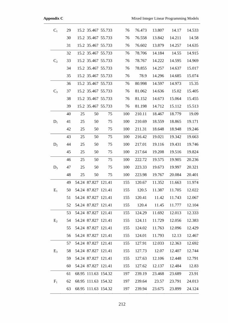
Appendix C Mixed Integer Linear Programming Models ______________________________________________________________________________________________________
C1 29 15.2 35.467 55.733 76 76.473 13.807 14.17 14.533
30 15.2 35.467 55.733 76 76.558 13.842 14.211 14.58
31 15.2 35.467 55.733 76 76.602 13.879 14.257 14.635
32 15.2 35.467 55.733 76 78.706 14.184 14.55 14.915
C2 33 15.2 35.467 55.733 76 78.767 14.222 14.595 14.969
34 15.2 35.467 55.733 76 78.855 14.257 14.637 15.017
35 15.2 35.467 55.733 76 78.9 14.296 14.685 15.074
36 15.2 35.467 55.733 76 80.998 14.597 14.973 15.35
C3 37 15.2 35.467 55.733 76 81.062 14.636 15.02 15.405
38 15.2 35.467 55.733 76 81.152 14.673 15.064 15.455
39 15.2 35.467 55.733 76 81.198 14.712 15.112 15.513
40 25 50 75 100 210.11 18.467 18.779 19.09
D1 41 25 50 75 100 210.69 18.559 18.865 19.171
42 25 50 75 100 211.31 18.648 18.948 19.246
43 25 50 75 100 216.42 19.021 19.342 19.663
D2 44 25 50 75 100 217.01 19.116 19.431 19.746
45 25 50 75 100 217.64 19.208 19.516 19.824
46 25 50 75 100 222.72 19.575 19.905 20.236
D3 47 25 50 75 100 223.33 19.673 19.997 20.321
48 25 50 75 100 223.98 19.767 20.084 20.401
49 54.24 87.827 121.41 155 120.67 11.352 11.663 11.974
E1 50 54.24 87.827 121.41 155 120.5 11.387 11.705 12.022
51 54.24 87.827 121.41 155 120.41 11.42 11.743 12.067
52 54.24 87.827 121.41 155 120.4 11.45 11.777 12.104
53 54.24 87.827 121.41 155 124.29 11.692 12.013 12.333
E2 54 54.24 87.827 121.41 155 124.11 11.729 12.056 12.383
55 54.24 87.827 121.41 155 124.02 11.763 12.096 12.429
56 54.24 87.827 121.41 155 124.01 11.793 12.13 12.467
57 54.24 87.827 121.41 155 127.91 12.033 12.363 12.692
E3 58 54.24 87.827 121.41 155 127.73 12.07 12.407 12.744
59 54.24 87.827 121.41 155 127.63 12.106 12.448 12.791
60 54.24 87.827 121.41 155 127.62 12.137 12.484 12.83
61 68.95 111.63 154.32 197 239.19 23.468 23.689 23.91
F1 62 68.95 111.63 154.32 197 239.64 23.57 23.791 24.013
63 68.95 111.63 154.32 197 239.94 23.675 23.899 24.124
212

Appendix C Mixed Integer Linear Programming Models ______________________________________________________________________________________________________
64 68.95 111.63 154.32 197 246.37 24.172 24.399 24.627
F2 65 68.95 111.63 154.32 197 246.83 24.277 24.505 24.734
66 68.95 111.63 154.32 197 247.13 24.385 24.616 24.848
67 68.95 111.63 154.32 197 253.55 24.876 25.11 25.345
F3 68 68.95 111.63 154.32 197 254.02 24.984 25.219 25.454
69 68.95 111.63 154.32 197 254.33 25.095 25.333 25.571
G1 70 140 210 280 350 132.08 11.397 11.612 11.826
G2 71 140 210 280 350 136.04 11.739 11.96 12.181
G3 72 140 210 280 350 140 12.081 12.308 12.535
H1 73 100 200 300 400 271.2 8.0741 8.4621 8.8501
74 100 200 300 400 272.91 8.0881 8.4781 8.8681
H2 75 100 200 300 400 279.34 8.3163 8.716 9.1156
76 100 200 300 400 281.1 8.3307 8.7324 9.1341
H3 77 100 200 300 400 287.47 8.5585 8.9698 9.3811
78 100 200 300 400 289.28 8.5734 8.9868 9.4002
213
References ____________________________________________________________________ (Alexandrov and Dennis, 1994) (Allan, 1995) (Anstine et al., 1963) (Baldick, 1995) (Bell et al., 1999) (Billinton and Allan, 1996) (Billinton and Karki, 1999) (Billinton and Li, 1994) (Bouffard, 2006) (Bouffard and Galiana, 2004) (Bouffard et al., 2005a) (Bouffard et al., 2005b) (Breipohl et al., 1992) (CAISO, 2005) (CEA, 1995) (CEA, 2004) (Chattopadhyay and Baldick, 2002) (Dash and Associates, 2005) (Debnath and Billinton, 1989) (Dillon et al., 1978) (Flynn et al., 2001) (GADS, 2005) (Gooi et al., 1999) (Grigg et al., 1999) (Gross and Galiana, 1987) (Guéret et al., 2000) (Han et al., 2001) (Hahn and Shapiro, 1967) (Hobbs et al., 1999) (IESO, 2004) (Kariuki and Allan, 1996) (Kim, 1997) (Kirschen, 2002) (Kirschen et al., 2003) (Kirschen and Strbac, 2004) (Koval and Chowdhury, 1994) (Lawton et al., 2003) (Madrigal and Quintana, 2000) (MathWorks, 2005) (Merlin and Sandrin, 1983) (NYISO, 2005) (Padhy, 2004) (Papoulis and Pillai, 2002) (Patton et al., 1988) (Peterson and Brammer, 1995) (PJM, 2004) (Ranaweera et al., 1997) (Rebours and Kirschen, 2005a) (Rebours and Kirschen, 2005b) (REE, 1998) (Strbac and Kirschen, 2000) (Sullivan et al., 1996) (Teisberg et al., (forthcoming)) (UCTE, 2005) (Wang and Shahidehpour, 1993) (Wang et al., 2005) (Williams, 1999) (Wood and Wollenberg, 1996) (Wu and Gooi, 1999) (Zhai et al., 1994) (Bunn, 2000) (Ortega-Vazquez et al., 2006, (forthcoming)) (Galiana et al., 2005) (Stoft, 2002) (NERC, 2006) (Calsetta et al., 1972)
References Alexandrov, N. and Dennis, J. E. J. (1994) Algorithms for bilevel optimization,
2005, Available from World Wide Web:
http://techreports.larc.nasa.gov/icase/1994/icase-1994-77.pdf
Allan, R. N. (1995), VOLL - fact or fiction, Power Engineering Journal, 9, 2-2.
Anstine, L. T., Burke, R. E., Casey, J. E., Holgate, R., John, R. S. and Stewart, H. G.
(1963), Application of probability methods to the determination of spinning
reserve requirements for the Pennsylvania-New Jersey-Maryland
interconnection, IEEE Trans. Power App. Syst., PAS-82, no. 68, 720-735.
Baldick, R. (1995), The generalized unit commitment problem, IEEE Trans. Power
Syst., 10, 465-475.
Bell, K., Rios, M., Kirschen, D. S. and Allan, R. (1999) Computation of the value of
security, Final Report, 1 UMIST, Available from World Wide Web:
http://www.umist.ac.uk/departments/mcee/research/publications.htm
Billinton, R. and Allan, R. N. (1996) Reliability Evaluation of Power Systems,
Plenum Press, New York; London.
Billinton, R. and Karki, R. (1999), Capacity reserve assessment using system well-
being analysis, IEEE Trans. Power Syst., 14, 433-438.
Billinton, R. and Li, W. (1994) Reliability Assessment of Electric Power Systems
using Monte Carlo Methods, Plenum, New York; London.
Bouffard, F. (2006), Electricity market-clearing with stochastic security, In Dep.
Elect. Comp. Eng., McGill Univ., Montreal, Quebec, pp. 1-200.
Bouffard, F. and Galiana, F. D. (2004), An electricity market with a probabilistic
spinning reserve criterion, IEEE Trans. Power Syst., 19, 300-307.
Bouffard, F., Galiana, F. D. and Conejo, A. J. (2005a), Market-clearing with
stochastic security - Part I: Formulation, IEEE Trans. Power Syst., 20, 1818-
1826.
214

References ____________________________________________________________________ Bouffard, F., Galiana, F. D. and Conejo, A. J. (2005b), Market-clearing with
stochastic security - Part II: Case studies, IEEE Trans. Power Syst., 20, 1827-
1835.
Breipohl, A. M., Lee, F. N., Zhai, D. and Adapa, R. (1992), A Gauss-Markov load
model for application in risk-evaluation and production simulation, IEEE
Trans. Power Syst., 7, 1493-1499.
Bunn, D. W. (2000), Forecasting loads and prices in competitive power markets,
Proceedings of the IEEE, 88, 163-169.
CAISO (2005) In Spinning Reserve Requirements, The California ISO, Available
from World Wide Web: http://www.caiso.com/
Calsetta, A. B., Albrecht, P., Cook, V. M., Ringlee, R., J. and Whooley, J. P. (1972),
A four-state model for estimation of outage risk for units in peaking service,
IEEE Trans. Power App. Syst., PAS-91, 618-627.
CEA (1995), Generation Equipment Status, Annual Report, Canadian Electricity
Association.
CEA (2004) Canadian Electricity Association, Available from World Wide Web:
http://www.canelect.ca/,
Chattopadhyay, D. and Baldick, R. (2002), Unit commitment with probabilistic
reserve, Proc. IEEE Power Engineering Society Winter Meeting, 1, 280-285.
Dash Associates (2005) Modeling with Xpress-MP, Dash Associates, Available from
World Wide Web:
http://www.dashoptimization.com/home/downloads/pdf/Modeling_with_Xpr
ess-MP.pdf
Debnath, K. and Billinton, R. (1989), Some aspects of generating-unit availability
models, IEEE Trans. Energy Conv., 4, 41-46.
Dillon, T. S., Edwin, K. W., Kochs, H. D. and Taud, R. J. (1978), Integer
programming approach to the problem of optimal unit commitment with
probabilistic reserve determination, IEEE Trans. Power App. Syst., 97, 2154-
2166.
Flynn, M., Sheridan, W. P., Dillon, J. D. and O'Malley, M. J. (2001), Reliability and
reserve in competitive electricity market scheduling, IEEE Trans. Power
Syst., 16, 78-87.
GADS (2005) Generating Availability Data System, Available from World Wide
Web: http://www.gadsnxl.com/
215

References ____________________________________________________________________ Galiana, F. D., Bouffard, F., Arroyo, J. M. and Restrepo, J. F. (2005), Scheduling
and pricing of coupled energy and primary, secondary, and tertiary reserves,
Proc. IEEE, 93, 1970-1983.
Gooi, H. B., Mendes, D. P., Bell, K. R. W. and Kirschen, D. S. (1999), Optimal
scheduling of spinning reserve, IEEE Trans. Power Syst., 14, 1485-1490.
Grigg, C., Wong, P., Albrecht, P., Allan, R., Bhavaraju, M., Billinton, R., Chen, Q.,
Fong, C., Haddad, S., Kuruganty, S., Li, W., Mukerji, R., Patton, D., Rau, N.,
Reppen, D., Schneider, A., Shahidehpour, M. and Singh, C. (1999), The
IEEE reliability test system - 1996, IEEE Trans. Power Syst., 14, 1010-1018.
Gross, G. and Galiana, F. D. (1987), Short-term load forecasting, Proceedings of the
IEEE, 75, 1558-1573.
Guéret, C., Prins, C. and Sevaux, M. (2000) Applications of Optimization with
Xpress-MP, (Ed, Eyrolles) Paris, France, Available from World Wide Web:
http://www.dashoptimization.com/home/downloads/book/booka4.pdf
Hahn, G. J. and Shapiro, S. S. (1967) Statistical Models in Engineering, John Wiley
& Sons, Inc.
Han, X. S., Gooi, H. B. and Kirschen, D. S. (2001), Dynamic economic dispatch:
Feasible and optimal solutions, IEEE Trans. Power Syst., 16, 22-28.
Hobbs, B. F., Jitprapaikulsarn, S., Konda, S., Chankong, V., Loparo, K. A. and
Maratukulam, D. J. (1999), Analysis of the value for unit commitment of
improved load forecasts, IEEE Trans. Power Syst., 14, 1342-1348.
IESO (2004) The Independent Electricity System Operator of Ontario Electrical
System, 2004, Available from World Wide Web: http://www.ieso.ca/
Kariuki, K. K. and Allan, R. N. (1996), Evaluation of reliability worth and value of
lost load, Proc. Inst. Elect. Eng., Gener., Transm., Distrib., 143, 171-180.
Kim, J. (1997), Iterated grid search algorithm on unimodal criteria, In Dept.
Statistics, Virginia Polytechnic Inst. and State Univ., Blacksburg, VA, pp. 1-
116.
Kirschen, D. S. (2002), Power system security, Power Eng. J., 16, 241-248.
Kirschen, D. S., Bell, K. R. W., Nedic, D. P., Jayaweera, D. and Allan, R. N. (2003),
Computing the value of security, Proc. Inst. Elect. Eng., Gener., Transm.,
Distrib., 150, 673-678.
Kirschen, D. S. and Strbac, G. (2004) Fundamentals of Power System Economics,
Wiley.
216

References ____________________________________________________________________ Koval, D. O. and Chowdhury, A. A. (1994), Generating peaking unit operating
characteristics, IEEE Trans. Ind. App., 30, 1309-1316.
Lawton, L., M., Sullivan, K., Van Liere, A., Katz, P. and Eto, J. (2003) A framework
and review of customer outage costs: integration and analysis of electric
utility outage cost surveys, Available from World Wide Web:
http://eetd.lbl.gov/EA/EMP/emp-pubsall.html
Madrigal, M. and Quintana, V. H. (2000), An analytical solution to the economic
dispatch problem, IEEE Power Engineering Review, 20, 52-55.
MathWorks (2005) MATLAB, 2005, Available from World Wide Web:
http://www.mathworks.com/access/helpdesk/help/techdoc/matlab.html?BB=
1
Merlin, A. and Sandrin, P. (1983), A new method for unit commitment at Electricité
de France, IEEE Trans. Power App. Syst., 102, 1218-1225.
NERC (2006) North American Electric Reliability Council, Available from World
Wide Web: http://www.nerc.com/
NYISO (2005) The New York Independent System Operator, New York, pp.
Demand Curves, Available from World Wide Web: http://www.nyiso.com
Ortega-Vazquez, M. A., Kirschen, D. S. and Pudjianto, D. (2006, (forthcoming)),
Optimal scheduling of spinning reserve considering the cost of interruptions,
Proc. Inst. Elect. Eng., Gener., Transm., Distrib.
Padhy, N. P. (2004), Unit commitment - A bibliographical survey, IEEE Trans.
Power Syst., 19, 1196-1205.
Papoulis, A. and Pillai, S. U. (2002) Probability, Random Variables and Stochastic
Processes, McGraw-Hill, New York; London.
Patton, A. D., Blackstone, J. H. and Balu, N. J. (1988), A Monte-Carlo simulation
approach to the reliability modeling of generating systems recognizing
operating considerations, IEEE Trans. Power Syst., 3, 1174-1180.
Peterson, W. L. and Brammer, S. R. (1995), A capacity based Lagrangian-relaxation
unit commitment with ramp rate constraints, IEEE Trans. Power Syst., 10,
1077-1083.
PJM (2004) In Scheduling Operation, Pennsylvania-New Jersey-Maryland,
Available from World Wide Web: http://www.pjm.com/contributions/pjm-
manuals/pdf/m11v22.pdf
217

References ____________________________________________________________________ Ranaweera, D. K., Karady, G. G. and Farmer, R. G. (1997), Economic impact
analysts of load forecasting, IEEE Trans. Power Syst., 12, 1388-1392.
Rebours, Y. and Kirschen, D. S. (2005a) A survey of definitions and specifications
of reserve services, 2005 UMIST, Manchester, Available from World Wide
Web: http://www.umist.ac.uk/departments/mcee/research/Publications/uom-
survey_reserve_services-2005.pdf
Rebours, Y. and Kirschen, D. S. (2005b) What is spinning reserve?, 2005 UMIST,
Manchester, Available from World Wide Web:
http://www.umist.ac.uk/departments/mcee/research/Publications/uom-
what_is_spinning_reserve-2005.pdf
REE (1998) In Operación del Sistema Eléctrico, Red Eléctrica de España, Available
from World Wide Web:
http://www.ree.es/cap03/pdf/po/PO_resol_30jul1998_b.pdf
Stoft, S. (2002) Power System Economics: Designing Markets for Electricity, IEEE-
Wiley, New York.
Strbac, G. and Kirschen, D. S. (2000), Who should pay for reserve?, The Electricity
Juornal, 32-37.
Sullivan, M. J., Vardell, T., Suddeth, B. N. and Vojdani, A. (1996), Interruption
costs, customer satisfaction and expectations for service reliability, IEEE
Trans. Power Syst., 11, 989-995.
Teisberg, T. J., Weiher, R. F. and Khotanzad, A. ( (forthcoming)), The value of
national weather service forecasts in scheduling electricity generation,
Bulletin of the American Meteorological Society.
UCTE (2005) Union for the Co-ordination of Transmission of Electricity Operation
Handbook, Available from World Wide Web:
http://www.ucte.org/pdf/ohb/Operation_Handbook_20.07.2004.pdf
Wang, C. and Shahidehpour, S. M. (1993), Effects of ramp-rate limits on unit
commitment and economic-dispatch, IEEE Trans. Power Syst., 8, 1341-1350.
Wang, J. X., Wang, X. F. and Wu, Y. (2005), Operating reserve model in the power
market, IEEE Trans. Power Syst., 20, 223-229.
Williams, H. P. (1999) Model Building in Mathematical Programming, Wiley,
Chichester.
Wood, A. J. and Wollenberg, B. F. (1996) Power Generation, Operation and
Control, Wiley, New York; Chichester.
218

References ____________________________________________________________________ Wu, H. and Gooi, H. B. (1999), Optimal scheduling of spinning reserve with ramp
constraints, Proc. IEEE Power Engineering Society Winter Meeting, 2, 785-
790.
Zhai, D., Breipohl, A. M., Lee, F. N. and Adapa, R. (1994), The effect of load
uncertainty on unit commitment risk, IEEE Trans. Power Syst., 9, 510-516.
219