Optimizing Portfolios - An Undergraduate Introduction …banach.millersville.edu/~bob/book/Optimal/main.pdf · Optimizing Portfolios An Undergraduate Introduction to Financial Mathematics

Optimizing PortfoliosAn Undergraduate Introduction to Financial Mathematics

J. Robert Buchanan

2010

J. Robert Buchanan Optimizing Portfolios

Introduction

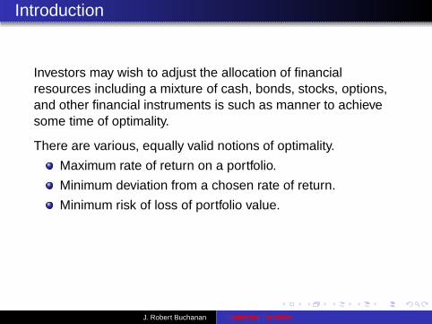
Investors may wish to adjust the allocation of financialresources including a mixture of cash, bonds, stocks, options,and other financial instruments is such as manner to achievesome time of optimality.

There are various, equally valid notions of optimality.

Maximum rate of return on a portfolio.

Minimum deviation from a chosen rate of return.

Minimum risk of loss of portfolio value.


Introduction

Investors may wish to adjust the allocation of financialresources including a mixture of cash, bonds, stocks, options,and other financial instruments is such as manner to achievesome time of optimality.

There are various, equally valid notions of optimality.

Maximum rate of return on a portfolio.

Minimum deviation from a chosen rate of return.

Minimum risk of loss of portfolio value.

The investor must choose the type of optimality they wish theirportfolio to have.


Covariance (1 of 2)

Definition

Covariance is a measure of the degree to which two randomvariables tend to change in the same or opposite directionrelative to one another. If X and Y are the random variablesthen the covariance, denoted Cov (X , Y ), is defined as

Cov (X , Y ) = E [(X − E [X ])(Y − E [Y ])] .


Covariance (2 of 2)

Theorem

If X and Y are random variables then

Cov (X , Y ) = E [XY ] − E [X ] E [Y ] .


Covariance (2 of 2)

Theorem

If X and Y are random variables then

Cov (X , Y ) = E [XY ] − E [X ] E [Y ] .

Cov (X , Y ) = E [XY − Y E [X ] − XE [Y ] + E [X ] E [Y ]]

= E [XY ]− E [Y ] E [X ] − E [X ] E [Y ] + E [X ] E [Y ]

= E [XY ]− E [X ] E [Y ]


Example (1 of 2)

Consider the following table listing the heights and armspans of20 children (source).

Child Ht. (cm) Span (cm) Child Ht. (cm) Span (cm)1 142 138 11 150 1472 148 144 12 152 1413 152 148 13 148 1444 150 145 14 152 1485 141 136 15 144 1406 142 139 16 148 1437 149 144 17 150 1468 151 145 18 138 1349 147 144 19 145 142

10 152 148 20 142 138

Find the covariance of height and armspan.


http://www.shodor.org/interactivate/discussions/GraphingData/

Example (2 of 2)

If X represents height and Y represents armspan then

E [X ] = 147.15

E [Y ] = 142.70

E [XY ] = 21013.8

which implies

Cov (X , Y ) = 21013.8 − (147.15)(142.70) = 15.445.

Note: since Cov (X , Y ) > 0, then in general as height increasesso does arm span.


Properties of Covariance (1 of 4)

Theorem

If X and Y are independent random variables thenCov (X , Y ) = 0.



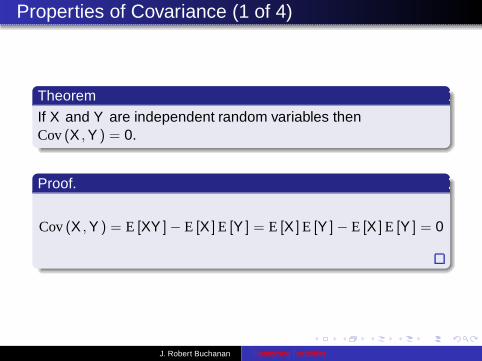
Theorem

If X and Y are independent random variables thenCov (X , Y ) = 0.

Proof.

Cov (X , Y ) = E [XY ]− E [X ] E [Y ] = E [X ] E [Y ] − E [X ] E [Y ] = 0



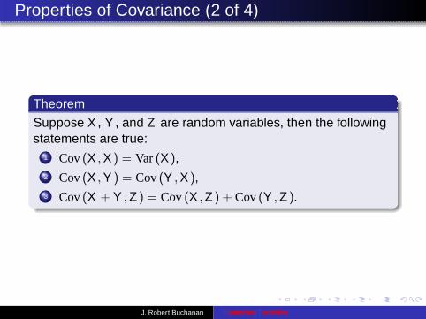
Theorem

Suppose X, Y , and Z are random variables, then the followingstatements are true:

1 Cov (X , X ) = Var (X ),2 Cov (X , Y ) = Cov (Y , X ),3 Cov (X + Y , Z ) = Cov (X , Z ) + Cov (Y , Z ).


Proof

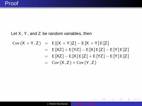
Let X , Y , and Z be random variables, then

Cov (X + Y , Z ) = E [(X + Y )Z ] − E [X + Y ] E [Z ]

= E [XZ ] + E [YZ ]− E [X ] E [Z ] − E [Y ] E [Z ]

= E [XZ ] − E [X ] E [Z ] + E [YZ ] − E [Y ] E [Z ]

= Cov (X , Z ) + Cov (Y , Z )



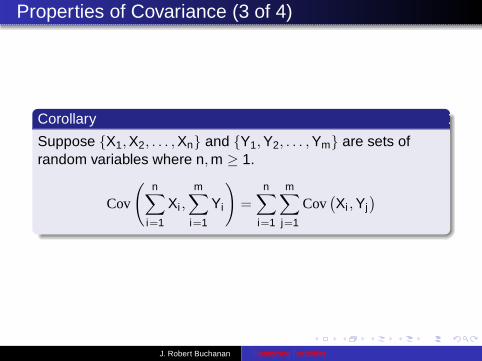
Corollary

Suppose {X1, X2, . . . , Xn} and {Y1, Y2, . . . , Ym} are sets ofrandom variables where n, m ≥ 1.

Cov

(

n∑

i=1

Xi ,m∑

i=1

Yi

)

=n∑

i=1

m∑

j=1

Cov(

Xi , Yj)


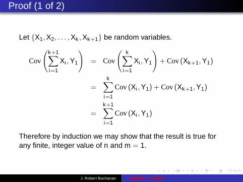
Proof (1 of 2)

Let {X1, X2, . . . , Xk , Xk+1} be random variables.

Cov

(

k+1∑

i=1

Xi , Y1

)

= Cov

(

k∑

i=1

Xi , Y1

)

+ Cov (Xk+1, Y1)

=

k∑

i=1

Cov (Xi , Y1) + Cov (Xk+1, Y1)

=

k+1∑

i=1

Cov (Xi , Y1)

Therefore by induction we may show that the result is true forany finite, integer value of n and m = 1.


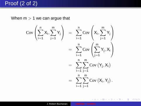
Proof (2 of 2)

When m > 1 we can argue that

Cov

n∑

i=1

Xi ,

m∑

j=1

Yj

=

n∑

i=1

Cov

Xi ,

m∑

j=1

Yj

=n∑

i=1

Cov

m∑

j=1

Yj , Xi

=

n∑

i=1

m∑

j=1

Cov(

Yj , Xi)

=

n∑

i=1

m∑

j=1

Cov(

Xi , Yj)

.



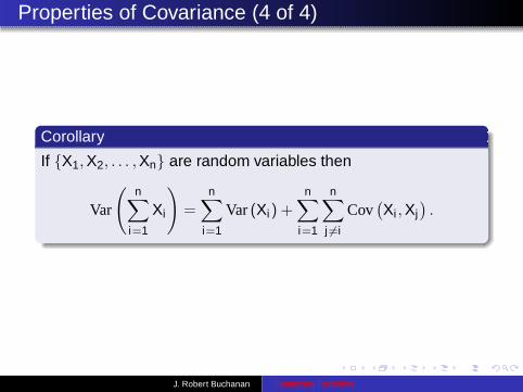
Corollary

If {X1, X2, . . . , Xn} are random variables then

Var

(

n∑

i=1

Xi

)

=n∑

i=1

Var (Xi) +n∑

i=1

n∑

j 6=i

Cov(

Xi , Xj)

.


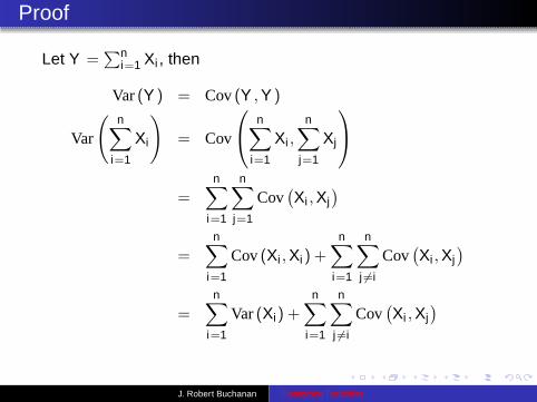
Proof

Let Y =∑n

i=1 Xi , then

Var (Y ) = Cov (Y , Y )

Var

(

n∑

i=1

Xi

)

= Cov

n∑

i=1

Xi ,n∑

j=1

Xj

=n∑

i=1

n∑

j=1

Cov(

Xi , Xj)

=n∑

i=1

Cov (Xi , Xi) +n∑

i=1

n∑

j 6=i

Cov(

Xi , Xj)

=n∑

i=1

Var (Xi) +n∑

i=1

n∑

j 6=i

Cov(

Xi , Xj)


Correlation

More informative than covariance would be information thatlarge changes in random variable X are accompanied by largechanges in Y .

Definition

If X and Y are random variables then the correlation of X andY denoted ρ (X , Y ) and defined as

ρ (X , Y ) =Cov (X , Y )

√

Var (X ) Var (Y ).


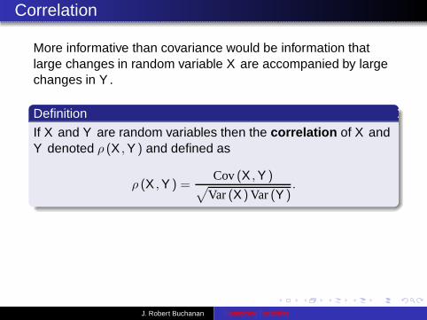
Correlation

More informative than covariance would be information thatlarge changes in random variable X are accompanied by largechanges in Y .

Definition

If X and Y are random variables then the correlation of X andY denoted ρ (X , Y ) and defined as

ρ (X , Y ) =Cov (X , Y )

√

Var (X ) Var (Y ).

Theorem

If X and Y are independent random variables thenρ (X , Y ) = 0. We say that X and Y are uncorrelated.


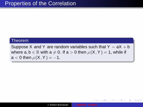
Properties of the Correlation

Theorem

Suppose X and Y are random variables such that Y = aX + bwhere a, b ∈ R with a 6= 0. If a > 0 then ρ (X , Y ) = 1, while ifa < 0 then ρ (X , Y ) = −1.


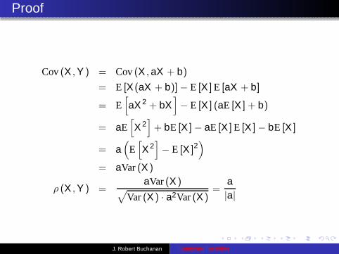
Proof

Cov (X , Y ) = Cov (X , aX + b)

= E [X (aX + b)] − E [X ] E [aX + b]

= E[

aX 2 + bX]

− E [X ] (aE [X ] + b)

= aE[

X 2]

+ bE [X ] − aE [X ] E [X ] − bE [X ]

= a(

E[

X 2]

− E [X ]2)

= aVar (X )

ρ (X , Y ) =aVar (X )

√

Var (X ) · a2Var (X )=

a|a|


Schwarz Inequality

We would like to prove that the correlation of two randomvariables is always in the interval [−1, 1]. First, we need thefollowing inequality.

Lemma (Schwarz Inequality)

If X and Y are random variables then(E [XY ])2 ≤ E

[

X 2]

E[

Y 2]

.


Proof (1 of 2)

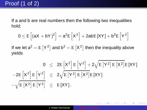
If a and b are real numbers then the following two inequalitieshold:

0 ≤ E[

(aX + bY )2]

= a2E[

X 2]

+ 2abE [XY ] + b2E[

Y 2]

If we let a2 = E[

Y 2]

and b2 = E[

X 2]

then the inequality aboveyields

0 ≤ 2E[

X 2]

E[

Y 2]

+ 2√

E[

Y 2]

E[

X 2]

E [XY ]

−2E[

X 2]

E[

Y 2]

≤ 2√

E[

Y 2]

E[

X 2]

E [XY ]

−√

E[

X 2]

E[

Y 2]

≤ E [XY ] .


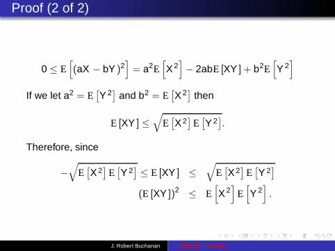
Proof (2 of 2)

0 ≤ E[

(aX − bY )2]

= a2E[

X 2]

− 2abE [XY ] + b2E[

Y 2]

If we let a2 = E[

Y 2]

and b2 = E[

X 2]

then

E [XY ] ≤√

E[

X 2]

E[

Y 2]

.

Therefore, since

−√

E[

X 2]

E[

Y 2]

≤ E [XY ] ≤√

E[

X 2]

E[

Y 2]

(E [XY ])2 ≤ E[

X 2]

E[

Y 2]

.


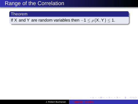
Range of the Correlation

Theorem

If X and Y are random variables then −1 ≤ ρ (X , Y ) ≤ 1.


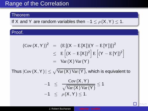
Range of the Correlation

Theorem

If X and Y are random variables then −1 ≤ ρ (X , Y ) ≤ 1.

Proof.

(Cov (X , Y ))2 = (E [(X − E [X ])(Y − E [Y ])])2

≤ E[

(X − E [X ])2]

E[

(Y − E [Y ])2]

= Var (X ) Var (Y )

Thus |Cov (X , Y ) | ≤√

Var (X ) Var (Y ), which is equivalent to

−1 ≤ Cov (X , Y )√

Var (X ) Var (Y )≤ 1

−1 ≤ ρ (X , Y ) ≤ 1.


Example

For the height and armspan data of the previous example,calculate the correlation between height and armspan.

140 142 144 146 148 150 152Height HcmL

136

138

140

142

144

146

148

Arm span HcmL


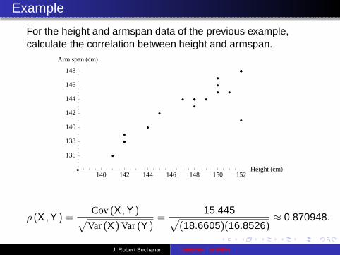
Example

For the height and armspan data of the previous example,calculate the correlation between height and armspan.

140 142 144 146 148 150 152Height HcmL

136

138

140

142

144

146

148

Arm span HcmL

ρ (X , Y ) =Cov (X , Y )

√

Var (X ) Var (Y )=

15.445√

(18.6605)(16.8526)≈ 0.870948.


Financial Example (1 of 2)

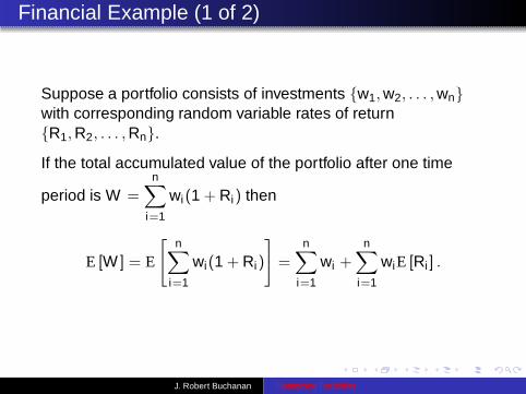
Suppose a portfolio consists of investments {w1, w2, . . . , wn}with corresponding random variable rates of return{R1, R2, . . . , Rn}.

If the total accumulated value of the portfolio after one time

period is W =

n∑

i=1

wi(1 + Ri) then

E [W ] = E

[

n∑

i=1

wi(1 + Ri)

]

=n∑

i=1

wi +n∑

i=1

wiE [Ri ] .


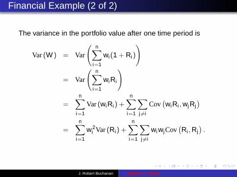
Financial Example (2 of 2)

The variance in the portfolio value after one time period is

Var (W ) = Var

(

n∑

i=1

wi(1 + Ri)

)

= Var

(

n∑

i=1

wiRi

)

=

n∑

i=1

Var (wiRi) +

n∑

i=1

∑

j 6=i

Cov(

wiRi , wjRj)

=

n∑

i=1

w2i Var (Ri) +

n∑

i=1

∑

j 6=i

wiwjCov(

Ri , Rj)

.


Technical Result

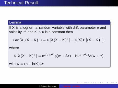
Lemma

If X is a lognormal random variable with drift parameter µ andvolatility σ2 and K > 0 is a constant then

Cov(

X , (X − K )+)

= E[

X (X − K )+]

− E [X ] E[

(X − K )+]

,

where

E[

X (X − K )+]

= e2(µ+σ2)φ(w + 2σ) − Keµ+σ2/2φ(w + σ),

with w = (µ − ln K )/σ.


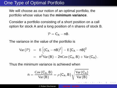
One Type of Optimal Portfolio

We will choose as our notion of an optimal portfolio, theportfolio whose value has the minimum variance.

Consider a portfolio consisting of a short position on a calloption for stock A and a long position of n shares of stock B.

P = CA − nB.

The variance in the value of the portfolio is

Var (P) = E[

(CA − nB)2]

− E [CA − nB]2

= n2Var (B) − 2nCov (CA, B) + Var (CA) .

Thus the minimum variance is achieved when

n =Cov (CA, B)

Var (B)= ρ (CA, B)

√

Var (CA)

Var (B).


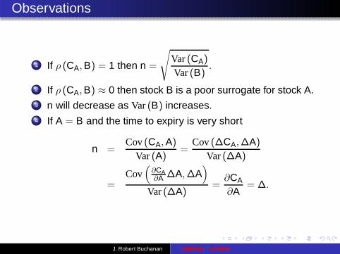
Observations

1 If ρ (CA, B) = 1 then n =

√

Var (CA)

Var (B).

2 If ρ (CA, B) ≈ 0 then stock B is a poor surrogate for stock A.3 n will decrease as Var (B) increases.4 If A = B and the time to expiry is very short

n =Cov (CA, A)

Var (A)=

Cov (∆CA,∆A)

Var (∆A)

=Cov

(

∂CA∂A ∆A,∆A

)

Var (∆A)=

∂CA

∂A= ∆.


An Introduction to Utility Functions

1 A utility function assigns to the outcomes of anexperiment, a value called the outcome’s utility.

2 Individual investors have differing utility functionscorresponding to their affinity for taking investment risks.

3 The utility function plays a role in making rationalinvestment decisions.


Assigning Utility to Outcomes (1 of 4)

Suppose there are n outcomes to an experiment

C1 ≤ C2 ≤ · · · ≤ Cn.

An investor can rank the outcomes in order of desirability.Suppose the outcomes have been ranked from least to mostdesirable as

C1 ≤ C2 ≤ · · · ≤ Cn.




C1 ≤ C2 ≤ · · · ≤ Cn.


C1 ≤ C2 ≤ · · · ≤ Cn.

Question: How is utility assigned to an outcome?




C1 ≤ C2 ≤ · · · ≤ Cn.


C1 ≤ C2 ≤ · · · ≤ Cn.

Question: How is utility assigned to an outcome?Answer: Let the utility function be u(x), then assignu(C1) = C1 and u(Cn) = Cn.



For 1 < i < n the investor is given a choice:1 participate in a random experiment in which the probability

of receiving Ci is 1, or2 participate in a random experiment where they receive C1

with probability φi and receive Cn with probability 1 − φi .



Note:

The expected value of the first experiment is Ci and theexpected value of the second experiment isφiC1 + (1 − φi)Cn.

By the Intermediate Value Theorem there exists φi ∈ [0, 1]such that

Ci = φiC1 + (1 − φi)Cn

thus define u(Ci) = φiC1 + (1 − φi)Cn.



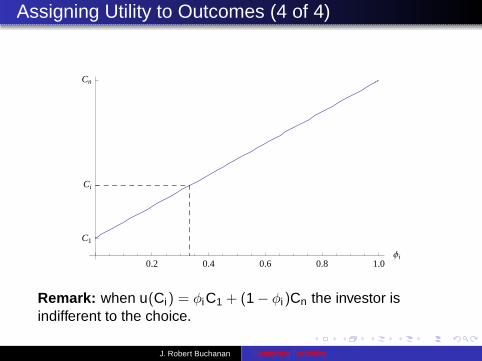
0.2 0.4 0.6 0.8 1.0Φi

C1

Ci

Cn

Remark: when u(Ci) = φiC1 + (1 − φi)Cn the investor isindifferent to the choice.


Application of the Utility Function

Suppose an investor must choose between two differentinvestment schemes. The union of all outcomes of the twoschemes is the set

{C1, C2, . . . , Cn}.The probability of receiving outcome Ci from the first scheme ispi and the probability of receiving it from the second is qi .

If the utility of the i th outcome is u(Ci) then the investor willchoose the first scheme is

n∑

i=1

piu(Ci) >

n∑

i=1

qiu(Ci).

In other words, the investor will choose the first scheme if theexpected value of its utility is greater than that of the secondscheme.


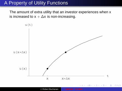
A Property of Utility Functions

The amount of extra utility that an investor experiences when xis increased to x + ∆x is non-increasing.

x x+Dxt

uHxL

uHx+DxL

uHtL


Concave Functions

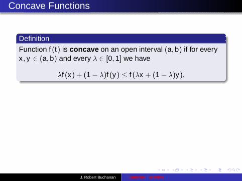
Definition

Function f (t) is concave on an open interval (a, b) if for everyx , y ∈ (a, b) and every λ ∈ [0, 1] we have

λf (x) + (1 − λ)f (y) ≤ f (λx + (1 − λ)y).


Concave Functions

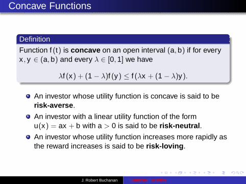
Definition

Function f (t) is concave on an open interval (a, b) if for everyx , y ∈ (a, b) and every λ ∈ [0, 1] we have

λf (x) + (1 − λ)f (y) ≤ f (λx + (1 − λ)y).

An investor whose utility function is concave is said to berisk-averse.

An investor with a linear utility function of the formu(x) = ax + b with a > 0 is said to be risk-neutral.

An investor whose utility function increases more rapidly asthe reward increases is said to be risk-loving.


Concavity and Derivatives

Theorem

If f ∈ C2(a, b) then f is concave on (a, b) if and only if f ′′(t) ≤ 0for a < t < b.


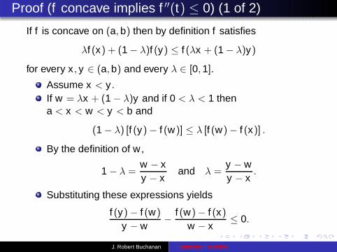
Proof (f concave implies f ′′(t) ≤ 0) (1 of 2)

If f is concave on (a, b) then by definition f satisfies

λf (x) + (1 − λ)f (y) ≤ f (λx + (1 − λ)y)

for every x , y ∈ (a, b) and every λ ∈ [0, 1].

Assume x < y .If w = λx + (1 − λ)y and if 0 < λ < 1 thena < x < w < y < b and

(1 − λ) [f (y) − f (w)] ≤ λ [f (w) − f (x)] .

By the definition of w ,

1 − λ =w − xy − x

and λ =y − wy − x

.

Substituting these expressions yields

f (y) − f (w)

y − w− f (w) − f (x)

w − x≤ 0.


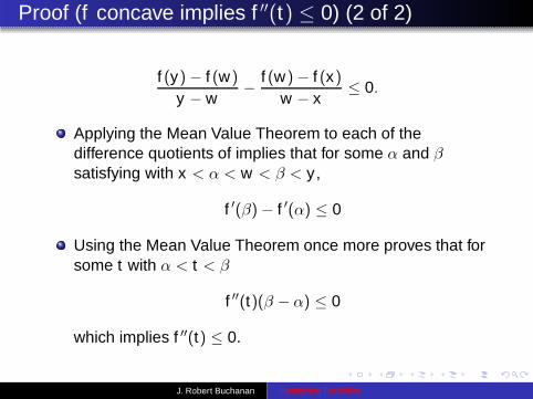
Proof (f concave implies f ′′(t) ≤ 0) (2 of 2)

f (y) − f (w)

y − w− f (w) − f (x)

w − x≤ 0.

Applying the Mean Value Theorem to each of thedifference quotients of implies that for some α and βsatisfying with x < α < w < β < y ,

f ′(β) − f ′(α) ≤ 0

Using the Mean Value Theorem once more proves that forsome t with α < t < β

f ′′(t)(β − α) ≤ 0

which implies f ′′(t) ≤ 0.


Jensen’s Inequality (Discrete Version)

Theorem (Jensen’s Inequality (Discrete Version))

Let f be a concave function on the interval (a, b), supposexi ∈ (a, b) for i = 1, 2, . . . , n, and suppose λi ∈ [0, 1] fori = 1, 2, . . . , n with

∑ni=1 λi = 1, then

n∑

i=1

λi f (xi) ≤ f

(

n∑

i=1

λixi

)

.


Jensen’s Inequality (Discrete Version) Proof

Let µ =∑n

i=1 λixi and note that since λi ∈ [0, 1] fori = 1, 2, . . . , n and

∑ni=1 λi = 1, then a < µ < b. The equation

of the line tangent to the graph of f at (µ, f (µ)) isy = f ′(µ)(x − µ) + f (µ). Since f is concave on (a, b) then

f (xi ) ≤ f ′(µ)(xi − µ) + f (µ) for i = 1, 2, . . . , n.

Therefore

n∑

i=1

λi f (xi) ≤n∑

i=1

(

λi[

f ′(µ)(xi − µ) + f (µ)])

= f ′(µ)

n∑

i=1

(λixi − λiµ) + f (µ)

n∑

i=1

λi

= f (µ) = f

(

n∑

i=1

λixi

)

.


Jensen’s Inequality (Continuous Version)

Theorem (Jensen’s Inequality (Continuous Version))

Let φ(t) be an integrable function on [0, 1] and let f be aconcave function, then

∫ 1

0f (φ(t)) dt ≤ f

(

∫ 1

0φ(t) dt

)

.


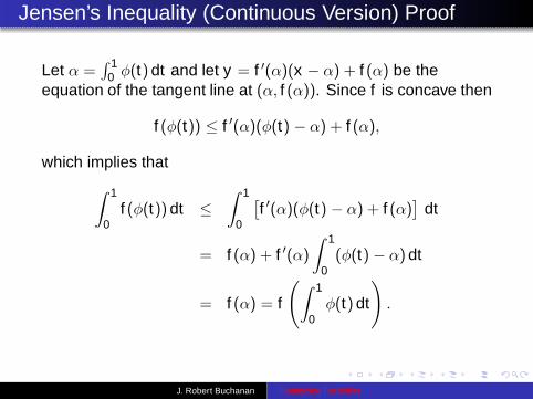
Jensen’s Inequality (Continuous Version) Proof

Let α =∫ 1

0 φ(t) dt and let y = f ′(α)(x − α) + f (α) be theequation of the tangent line at (α, f (α)). Since f is concave then

f (φ(t)) ≤ f ′(α)(φ(t) − α) + f (α),

which implies that

∫ 1

0f (φ(t)) dt ≤

∫ 1

0

[

f ′(α)(φ(t) − α) + f (α)]

dt

= f (α) + f ′(α)

∫ 1

0(φ(t) − α) dt

= f (α) = f

(

∫ 1

0φ(t) dt

)

.


Expected Utility

Definition

The expected value of a utility function is called its expectedutility.


Expected Utility

Definition

The expected value of a utility function is called its expectedutility.

Example

An investor is risk-averse with a utility functionu(x) = x − x2/25. The investor must choose between thefollowing two “investments”:

A: Flip a fair coin, if the coin lands heads up theinvestor receives $10, otherwise they receivenothing.

B: Receive an amount $M with certainty.

Which do they choose?


Solution

A rational investor will select the investment with the greaterexpected utility.


Solution

A rational investor will select the investment with the greaterexpected utility.The expected utility for investment A is

12

u(10) +12

u(0) =12

(

10 − 102

25

)

= 3.


Solution

A rational investor will select the investment with the greaterexpected utility.The expected utility for investment A is

12

u(10) +12

u(0) =12

(

10 − 102

25

)

= 3.

The expected utility for B is u(M) = M − M2/25. Thus theinvestor will choose the coin flip whenever

3 > M − M2

25

Thus investment A is preferable to B whenever M < $3.49.


Certainty Equivalent

Definition

The certainty equivalent is the minimum value C of a randomvariable X for which u(C) = E [u(X )].


Certainty Equivalent

Definition

The certainty equivalent is the minimum value C of a randomvariable X for which u(C) = E [u(X )].

Example

An investor is risk-averse with a utility functionu(x) = x − x2/25. The investor wishes to find the certaintyequivalent C for the following investment choice:

A: Flip a fair coin, if the coin lands heads up theinvestor receives 0 < X ≤ 10, otherwise theyreceive 0 < Y < X .

B: Receive an amount C with certainty.


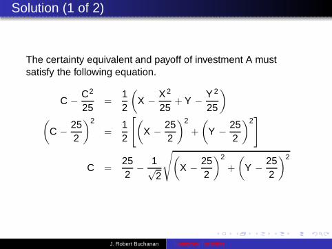
Solution (1 of 2)

The certainty equivalent and payoff of investment A mustsatisfy the following equation.

C − C2

25=

12

(

X − X 2

25+ Y − Y 2

25

)

(

C − 252

)2

=12

[

(

X − 252

)2

+

(

Y − 252

)2]

C =252

− 1√2

√

(

X − 252

)2

+

(

Y − 252

)2


Solution (2 of 2)

0

5

10

X

0

5

10

Y

0

5

10

C


Portfolio Selection (1 of 2)

We wish to examine the problem of allocating resources amongpotentially many different investments in an optimal fashion.

Consider a simple case:

An investor has x capital to invest.

The investor allocates fraction α ∈ [0, 1] to an investment.

The investment is structured such that an allocation of αxwill earn αx with probability p and lose αx with probability1 − p.


Portfolio Selection (2 of 2)

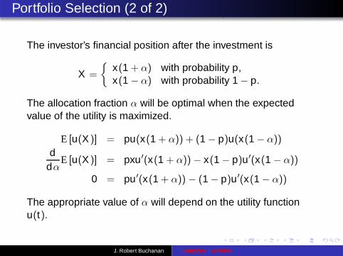
The investor’s financial position after the investment is

X =

{

x(1 + α) with probability p,x(1 − α) with probability 1 − p.

The allocation fraction α will be optimal when the expectedvalue of the utility is maximized.

E [u(X )] = pu(x(1 + α)) + (1 − p)u(x(1 − α))

ddα

E [u(X )] = pxu′(x(1 + α)) − x(1 − p)u′(x(1 − α))

0 = pu′(x(1 + α)) − (1 − p)u′(x(1 − α))

The appropriate value of α will depend on the utility functionu(t).


General Portfolio Selection Problem

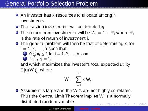
An investor has x resources to allocate among ninvestments.The fraction invested in i will be denoted xi .The return from investment i will be Wi = 1 + Ri where Ri

is the rate of return of investment i .The general problem will then be that of determining xi fori = 1, 2, . . . , n such that

1 0 ≤ xi ≤ 1 for i = 1, 2, . . . , n, and2∑n

i=1 xi = 1,and which maximizes the investor’s total expected utilityE [u(W )], where

W =

n∑

i=1

xiWi .

Assume n is large and the Wi ’s are not highly correlated.Thus the Central Limit Theorem implies W is a normallydistributed random variable.


Example (1 of 3)

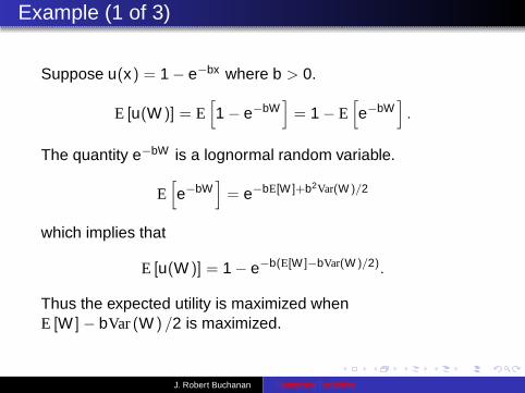
Suppose u(x) = 1 − e−bx where b > 0.

E [u(W )] = E[

1 − e−bW]

= 1 − E[

e−bW]

.

The quantity e−bW is a lognormal random variable.

E[

e−bW]

= e−bE[W ]+b2Var(W )/2

which implies that

E [u(W )] = 1 − e−b(E[W ]−bVar(W )/2).

Thus the expected utility is maximized whenE [W ] − bVar (W ) /2 is maximized.


Example (2 of 3)

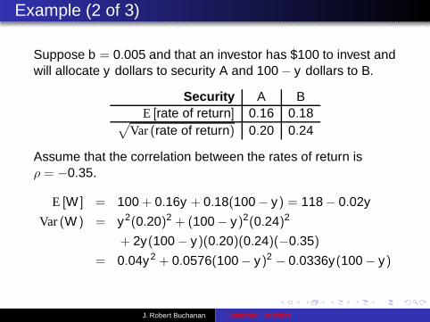
Suppose b = 0.005 and that an investor has $100 to invest andwill allocate y dollars to security A and 100 − y dollars to B.

Security A BE [rate of return] 0.16 0.18

√

Var (rate of return) 0.20 0.24

Assume that the correlation between the rates of return isρ = −0.35.

E [W ] = 100 + 0.16y + 0.18(100 − y) = 118 − 0.02y

Var (W ) = y2(0.20)2 + (100 − y)2(0.24)2

+ 2y(100 − y)(0.20)(0.24)(−0.35)

= 0.04y2 + 0.0576(100− y)2 − 0.0336y(100 − y)


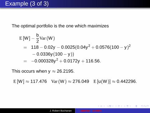
Example (3 of 3)

The optimal portfolio is the one which maximizes

E [W ] − b2

Var (W )

= 118 − 0.02y − 0.0025(0.04y2 + 0.0576(100− y)2

− 0.0336y(100− y))

= −0.000328y2 + 0.0172y + 116.56.

This occurs when y ≈ 26.2195.

E [W ] ≈ 117.476 Var (W ) ≈ 276.049 E [u(W )] ≈ 0.442296.


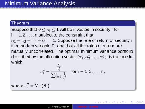
Minimum Variance Analysis

Theorem

Suppose that 0 ≤ αi ≤ 1 will be invested in security i fori = 1, 2, . . . , n subject to the constraint thatα1 + α2 + · · · + αn = 1. Suppose the rate of return of security iis a random variable Ri and that all the rates of return aremutually uncorrelated. The optimal, minimum variance portfoliodescribed by the allocation vector 〈α∗

1, α∗2, . . . , α

∗n〉, is the one for

which

α∗i =

1σ2

i∑n

j=11σ2

j

for i = 1, 2, . . . , n,

where σ2i = Var (Ri).


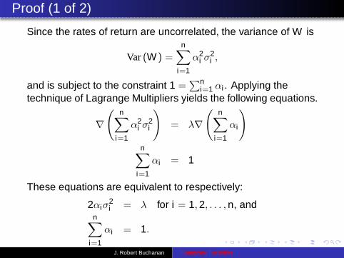
Proof (1 of 2)

Since the rates of return are uncorrelated, the variance of W is

Var (W ) =n∑

i=1

α2i σ

2i ,

and is subject to the constraint 1 =∑n

i=1 αi . Applying thetechnique of Lagrange Multipliers yields the following equations.

∇(

n∑

i=1

α2i σ

2i

)

= λ∇(

n∑

i=1

αi

)

n∑

i=1

αi = 1

These equations are equivalent to respectively:

2αiσ2i = λ for i = 1, 2, . . . , n, and

n∑

i=1

αi = 1.


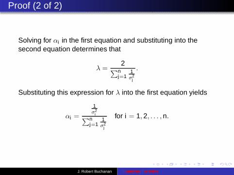
Proof (2 of 2)

Solving for αi in the first equation and substituting into thesecond equation determines that

λ =2

∑nj=1

1σ2

j

.

Substituting this expression for λ into the first equation yields

αi =

1σ2

i∑n

j=11σ2

j

for i = 1, 2, . . . , n.


Including the Effects of Borrowing

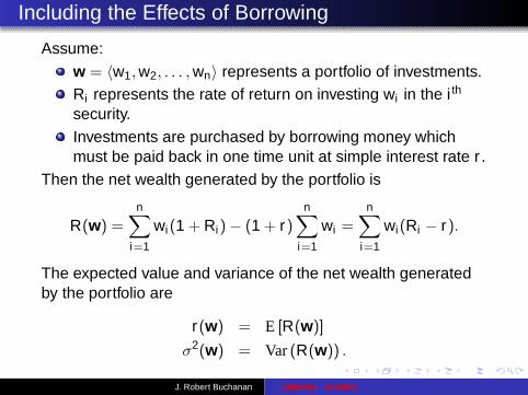
Assume:

w = 〈w1, w2, . . . , wn〉 represents a portfolio of investments.Ri represents the rate of return on investing wi in the i th

security.Investments are purchased by borrowing money whichmust be paid back in one time unit at simple interest rate r .

Then the net wealth generated by the portfolio is

R(w) =

n∑

i=1

wi(1 + Ri) − (1 + r)n∑

i=1

wi =

n∑

i=1

wi(Ri − r).

The expected value and variance of the net wealth generatedby the portfolio are

r(w) = E [R(w)]

σ2(w) = Var (R(w)) .


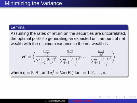
Minimizing the Variance

Lemma

Assuming the rates of return on the securities are uncorrelated,the optimal portfolio generating an expected unit amount of netwealth with the minimum variance in the net wealth is

w∗ =

⟨ r1−rσ2

1∑n

j=1(rj−r)2

σ2j

,

r2−rσ2

2∑n

j=1(rj−r)2

σ2j

, . . . ,

rn−rσ2

n∑n

j=1(rj−r)2

σ2j

⟩

where ri = E [Ri ] and σ2i = Var (Ri) for i = 1, 2, . . . , n.


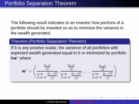
Portfolio Separation Theorem

The following result indicates to an investor how portions of aportfolio should be invested so as to minimize the variance inthe wealth generated.

Theorem (Portfolio Separation Theorem)

If b is any positive scalar, the variance of all portfolios withexpected wealth generated equal to b is minimized by portfoliobw∗ where

w∗ =

⟨ r1−rσ2

1∑n

j=1(rj−r)2

σ2j

,

r2−rσ2

2∑n

j=1(rj−r)2

σ2j

, . . . ,

rn−rσ2

n∑n

j=1(rj−r)2

σ2j

⟩


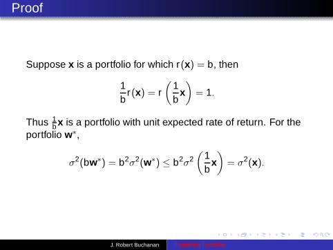
Proof

Suppose x is a portfolio for which r(x) = b, then

1b

r(x) = r(

1b

x)

= 1.

Thus 1b x is a portfolio with unit expected rate of return. For the

portfolio w∗,

σ2(bw∗) = b2σ2(w∗) ≤ b2σ2(

1b

x)

= σ2(x).


Risky vs. Risk Free Investments

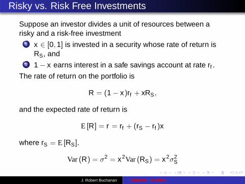
Suppose an investor divides a unit of resources between arisky and a risk-free investment

1 x ∈ [0, 1] is invested in a security whose rate of return isRS, and

2 1 − x earns interest in a safe savings account at rate rf .

The rate of return on the portfolio is

R = (1 − x)rf + xRS ,

and the expected rate of return is

E [R] = r = rf + (rS − rf )x

where rS = E [RS].

Var (R) = σ2 = x2Var (RS) = x2σ2S


Linear Relationship

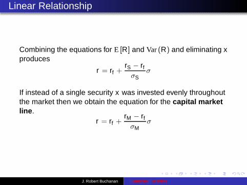
Combining the equations for E [R] and Var (R) and eliminating xproduces

r = rf +rS − rf

σSσ

If instead of a single security x was invested evenly throughoutthe market then we obtain the equation for the capital marketline.

r = rf +rM − rf

σMσ


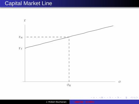
Capital Market Line

ΣM

Σ

rf

rM

r


Capital Assets Pricing Model (1 of 4)

Suppose an investor wishes to weigh the return on aninvestment against the risk associated with the investment.

Ri : return on investment in security i

RM : return on the entire market

x : fraction of unit wealth invested in security i

1 − x : fraction of unit wealth invested in market

The rate of return on the portfolio is

R = xRi + (1 − x)RM ,

with

E [R] = xE [Ri ] + (1 − x)E [RM ]

Var (R) = x2Var (Ri) + (1 − x)2Var (RM) + 2x(1 − x)Cov (Ri , RM) .



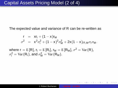
The expected value and variance of R can be re-written as

r = xri + (1 − x)rM

σ2 = x2σ2i + (1 − x)2σ2

M + 2x(1 − x)ρi ,MσiσM .

where r = E [R], ri = E [Ri ], rM = E [RM ], σ2 = Var (R),σ2

i = Var (Ri), and σ2M = Var (RM).



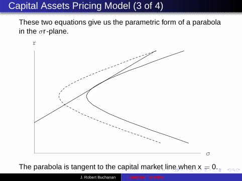
These two equations give us the parametric form of a parabolain the σr -plane.

Σ

r

The parabola is tangent to the capital market line when x = 0.J. Robert Buchanan Optimizing Portfolios


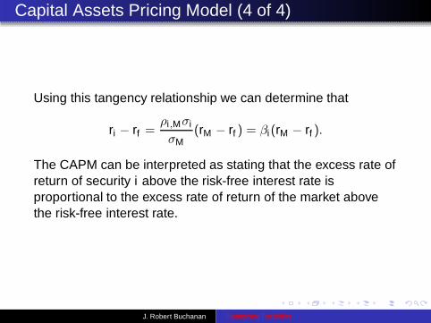
Using this tangency relationship we can determine that

ri − rf =ρi ,Mσi

σM(rM − rf ) = βi(rM − rf ).

The CAPM can be interpreted as stating that the excess rate ofreturn of security i above the risk-free interest rate isproportional to the excess rate of return of the market abovethe risk-free interest rate.


Example

Example

Suppose the risk-free interest rate is 5% per year, the return onthe market is 9% per year, and the volatility in the market is35% per year. Suppose further that the covariance between thereturn on a particular stock and the return on the market is0.10. Estimate the return on the stock.


Example

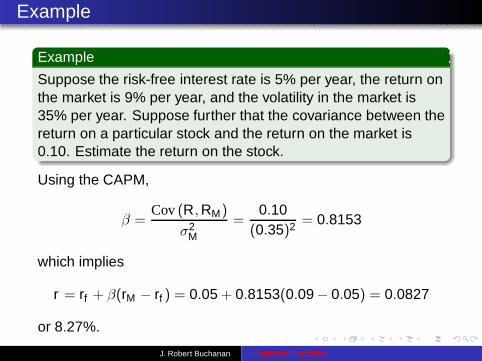
Example

Suppose the risk-free interest rate is 5% per year, the return onthe market is 9% per year, and the volatility in the market is35% per year. Suppose further that the covariance between thereturn on a particular stock and the return on the market is0.10. Estimate the return on the stock.

Using the CAPM,

β =Cov (R, RM)

σ2M

=0.10

(0.35)2 = 0.8153

which implies

r = rf + β(rM − rf ) = 0.05 + 0.8153(0.09 − 0.05) = 0.0827

or 8.27%.


Documents

Optimizing Portfolios - An Undergraduate Introduction …banach.millersville.edu/~bob/book/Optimal/main.pdf · Optimizing Portfolios An Undergraduate Introduction to Financial Mathematics