Optimizing Non-Local Pixel Predictors for Reversible …staff.ustc.edu.cn/~zhangwm/Paper/2014_3.pdfPixel Predictors for Reversible Data Hiding ... of the differences ... be saved for

International Journal of Digital Crime and Forensics, 6(3), 1-15, July-September 2014 1

Copyright © 2014, IGI Global. Copying or distributing in print or electronic forms without written permission of IGI Global is prohibited.

ABSTRACTThis paper presents a two-step clustering and optimizing pixel prediction method for reversible data hiding, which exploits self-similarities and group structural information of non-local image patches. Pixel predictors play an important role for current prediction-error expansion (PEE) based reversible data hiding schemes. Instead of using a fixed or a content- adaptive predictor for each pixel independently, the authors first employ pixel clustering according to the structural similarities of image patches, and then for all the pixels assigned to each cluster, an optimized pixel predictor is estimated from the group context. Experimental results demonstrate that the proposed method outperforms state-of-art counterparts such as the simple rhombus neighborhood, the median edge detector, and the gradient-adjusted predictor et al.

Optimizing Non-Local Pixel Predictors for

Reversible Data HidingXiaocheng Hu, School of Information Science and Technology, University of Science

and Technology of China, Hefei, China

Weiming Zhang, School of Information Science and Technology, University of Science and Technology of China, Hefei, China

Nenghai Yu, School of Information Science and Technology, University of Science and Technology of China, Hefei, China

Keywords: Clustering, L1-Norm Optimization, Pixel Prediction, Reversible Data Hiding, Self-Similarities

INTRODUCTION

As a technique that embeds messages into cover signals, information hiding has been widely applied in areas such

as convert communication, copyright protection and media annotation. Re-versible data hiding (RDH), as a special type of information hiding technique, has received much attention from the

DOI: 10.4018/ijdcf.2014070101


2 International Journal of Digital Crime and Forensics, 6(3), 1-15, July-September 2014

information community (Shi, Ni, Zou, Liang, & Xuan, 2004; Shi, 2004; Calde-lli, Filippini, & Becarelli, 2010) in the last decade. Specifically, RDH ensures not only the embedded messages shall be extracted precisely, but also the cover itself should be restored losslessly. This property is important in some special scenarios such as medical imagery (Bao et al., 2005), military imagery and law forensics. In these applications, the cover is too precious or too important to be damaged (Feng et al., 2006). Moreover, it has been found recently that revers-ible data hiding can be quite helpful in video error-concealment coding (Chung et al., 2010).

A plenty of reversible data hiding algorithms have been proposed in the past decade. Classical RDH methods roughly fall into three categories. The first class of algorithms follows the idea of compression-embedding framework, which was first introduced by Fridrich, Goljan, and Du (2002). In these algorithms, a two-value feature is calculated for each pixel group, the sequence is compressible and messages can be embedded in the extra space left by lossless compression. The send class of techniques is based on difference expansion (DE) (Tian, 2003; Thodi & Rodriguez, 2007), in which the differ-ences of each pixel groups are expanded, e.g., multiplied by 2, and thus the least significant bits (LSBs) of the differences are all-zeros and can be used for embed-ding messages. The last RDH schemes are based on histogram shift (HS) (Ni, Shi, Ansari, & Wei, 2006). The histogram

of one special feature (for example, gray-scale value) of the nature image is quite uneven, which implies that the histogram can be modified for embed-ding data. For instance some space can be saved for watermarks by shifting the bins of histogram.

In fact, by applying DE of HS to the residual part of nature images instead, e.g., the prediction errors (PE) (Tsai, Hu, & Yeh, 2009; Luo et al., 2010; Peng, Li, & Yang, 2012; Li, Yang, & Zeng, 2011), better performance can be achieved. This extended method is called prediction-error expansion (PEE), which is currently a research hotspot and the most powerful technique of RDH. Unlike in DE where only the correlation of two adjacent pix-els is considered, the local correlation of larger neighborhood is exploited in PEE. Most recently proposed RDH works are based on PEE by incorporating some strategies such as better prediction algo-rithm utilization (Sachnev, Kim, Nam, Suresh, & Shi, 2009; Fallahpour, 2008; Yang, Chung, Liao, & Yu, 2013; Ou, Li, Zhao, & Ni, 2013), double-layered embedding (Luo et al., 2010; Sachnev et al., 2009), embedding position selection (Li et al., 2011), context modification (Coltuc, 2011), optimal bins selection (Wang, Li, & Yang, 2010; Wu & Huang, 2012), etc.

Almost all recent PEE based meth-ods consist of two steps. The first step generates a host sequence with small entropy, i.e., the host has a sharp histo-gram, which usually can be realized by using PE combined with better prediction strategies. The second step reversibly



embeds messages into the host sequence by modifying its histogram with method like HS and DE. The performance of the overall embedding scheme is directly influenced by the accuracy of predic-tion, the steeper the prediction errors histogram is, the better the embedding performance can be achieved. Typical prediction methods either use a fixed neighborhood average model (Sachnev et al., 2009), or a content adaptive pre-dictor such as the median edge detector (MED) predictor (Thodi & Rodriguez, 2007) and the gradient-adjusted pre-dictor (GAP) (Fallahpour, 2008). They treat each pixel independently while structural self-similarities of non-local image patches are rarely considered.

In this paper, we proposed to first divide all pixels into several clusters according to the patch-level structural similarities of their prediction context by means of clustering, as shown in Figure 1. Afterwards, for all the pixels assigned to

each cluster, an optimized pixel predic-tor is estimated from the group context. Each pixel is predicted by a weighted linear combination of its nearest eight neighbors, and a quad- layered embed-ding scheme is proposed to traverse all the pixels in the cover image.

The rest of the paper is organized as follows. Section II gives a brief review to the PEE method. The proposed two-step clustering and optimizing scheme is presented in Section III. Experimental results compared to other pixel predic-tors are demonstrated in Section IV. And finally, Section V concludes this paper and discusses future research directions.

PREDICTION-ERROR EXPANSION (PEE)

Typical PEE based schemes divide cover image pixels into different parts, while a pixel of one part is predicted by its neighboring pixels in other parts.

Figure 1. Pixel clustering based on structural self-similarities of image patches



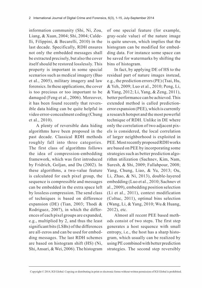
Take the rhombus pattern in Sachnev et al.’s double-layered embedding method (2009) for instance, in which all pixels are divided into two sets: the Cross set and the Dot set (see Figure 2). In the first round, the Cross set is used for em-bedding data and Dot set for computing predictions, while in the second round, the Dot set is used for embedding and Cross set for computing predictions. Since the two layers’ embedding pro-cesses are similar in nature, we only take the Cross layer for illustration.

As shown in Figure 2, the Cross pixels u

i j, in the cover image are col-

lected into a sequence u = ( , , , )u u un1 2

� from left to right and from top to bottom. For each Cross pixel u

i j,, the rhombus

predicted value ui j� , is computed using its four nearest Dot pixels:

uv v v v

i ji j i j i j i j�

,, , , ,=+ + +

− + + −1 1 1 1

4

(1)

Then, by subtracting the predicted value ui j� , from the original pixel value ui j,

, we obtain the prediction-error se-quence e = ( , , , )e e e

n1 2� . Afterwards,

secret data are embedded into the pre-diction-error sequence e through ex-panding and shifting. Specifically, for each e

i, it is expanded or shifted as:

e

e m e T T

e T e T

ei

i i n p

i p i p

i

'

, [ , ]

, ( , )=+ ∈

+ + ∈ +∞2

1

if

if

++ ∈ −∞

T e T

n i n, ( , ) if

(2)

where Tn< 0 and T

p≥ 0 are capacity-

dependent integer valued parameter, and

Figure 2. Rhombus prediction pattern. The pixel value of u of the Cross set can be pre-dicted by using the four neighboring pixel values of the Dot set and expanded to hide one bit of data



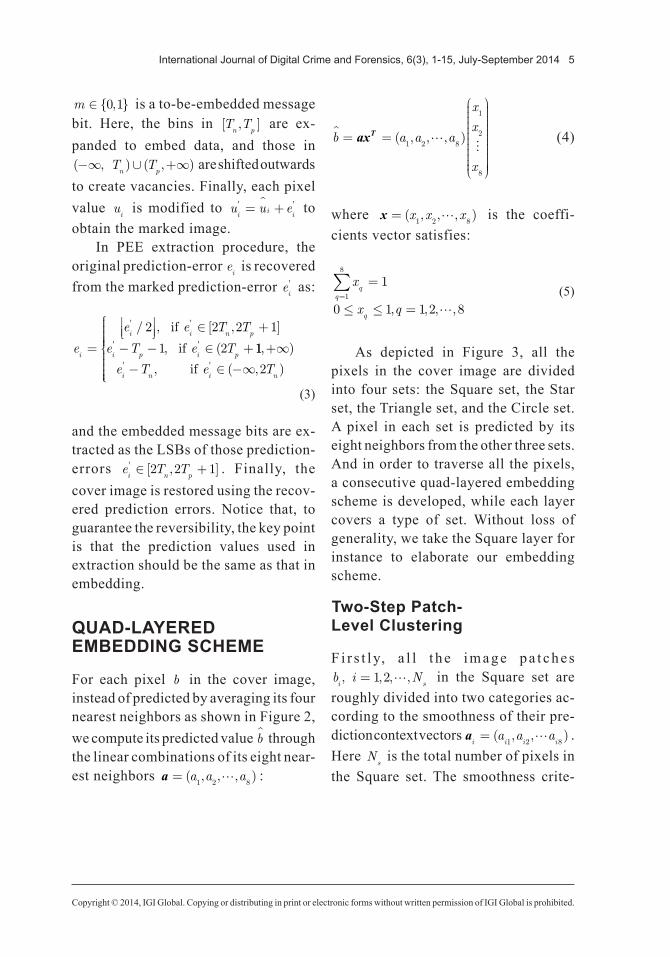
m ∈ { , }0 1 is a to-be-embedded message bit. Here, the bins in [ , ]T T

n p are ex-

panded to embed data, and those in ( ) ( ), ,−∞ +∞∪ T T

n p are shifted outwards

to create vacancies. Finally, each pixel value u

i is modified to u u e

i i i' '= +� to

obtain the marked image.In PEE extraction procedure, the

original prediction-error ei is recovered

from the marked prediction-error ei' as:

e

e e T T

e T e Ti

i i n p

i p i p=

∈ +

− − ∈ +

' '

' '

/ , [ , ]

, (

2 2 2 1

1 2

if

if 11

2

, )

, ( , )' '

+∞

− ∈ −∞

e T e Ti n i n

if

(3)

and the embedded message bits are ex-tracted as the LSBs of those prediction-errors e T T

i n p' [ , ]∈ +2 2 1 . Finally, the

cover image is restored using the recov-ered prediction errors. Notice that, to guarantee the reversibility, the key point is that the prediction values used in extraction should be the same as that in embedding.

QUAD-LAYERED EMBEDDING SCHEME

For each pixel b in the cover image, instead of predicted by averaging its four nearest neighbors as shown in Figure 2, we compute its predicted value b� through the linear combinations of its eight near-est neighbors a = ( , , , )a a a

1 2 8� :

b a a a

x

x

x

� ��

= =

axT ( , , , )1 2 8

1

2

8

(4)

where x = ( , , , )x x x1 2 8� is the coeffi-

cients vector satisfies:

x

x q

qq

q

=∑ =

≤ ≤ =1

8

1

0 1 1 2 8, , , ,� (5)

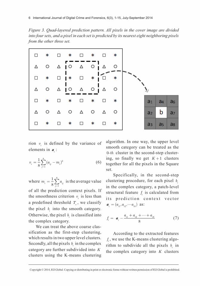
As depicted in Figure 3, all the pixels in the cover image are divided into four sets: the Square set, the Star set, the Triangle set, and the Circle set. A pixel in each set is predicted by its eight neighbors from the other three sets. And in order to traverse all the pixels, a consecutive quad-layered embedding scheme is developed, while each layer covers a type of set. Without loss of generality, we take the Square layer for instance to elaborate our embedding scheme.

Two-Step Patch-Level Clustering

F i r s t l y, a l l t h e im ag e p a t c h es b i Ni s, , , , = 1 2� in the Square set are

roughly divided into two categories ac-cording to the smoothness of their pre-diction context vectors a

i i i ia a a= ( , , )

1 2 8� .

Here Ns is the total number of pixels in

the Square set. The smoothness crite-



rion vi is defined by the variance of

elements in ai:

v a mi ij i

j

= −=∑1

82

1

8

( ) (6)

where m ai ij

j

==∑1

8 1

8

is the average value

of all the prediction context pixels. If the smoothness criterion v

i is less than

a predefined threshold Tv

, we classify the pixel b

i into the smooth category.

Otherwise, the pixel bi is classified into

the complex category.We can treat the above coarse clas-

sification as the first-step clustering, which results in two upper level clusters. Secondly, all the pixels b

i in the complex

category are further subdivided into K clusters using the K-means clustering

algorithm. In one way, the upper level smooth category can be treated as the 0-th cluster in the second-step cluster-ing, so finally we get K +1 clusters together for all the pixels in the Square set.

Specifically, in the second-step clustering procedure, for each pixel b

i

in the complex category, a patch-level structural feature f

i is calculated from

i t s p r e d i c t i o n c o n t e x t v e c t o r ai i i ia a a= ( , , )

1 2 8� as:

fa a a

i ii i i= −+ + +

a 1 2 8

8

� (7)

According to the extracted features fi, we use the K-means clustering algo-

rithm to subdivide all the pixels bi in

the complex category into K clusters

Figure 3. Quad-layered prediction pattern. All pixels in the cover image are divided into four sets, and a pixel in each set is predicted by its nearest eight neighboring pixels from the other three set.



as depicted in Figure 1. Here K is a predefined parameter for the K-means algorithm. Note that the initial cluster centroid pixel indexes for the K-means algorithm are selected every S pixels starting from the S th- pixel, namely S S KS, , ,2 � . And the interval parameter S is transmitted to the receiver side for the sake of repeating the K-means algo-rithm.

Optimizing Non-Local Pixel Predictors

In the two-step clustering procedure d e s c r i b e d a b o v e , a l l p i x e l s b i Ni s, , , , = 1 2� in the Square set are

classified into K +1 clusters. After that, for all the pixels b j c c c

j Nk, , , ,=

1 2� as-

signed to a specified cluster, a content adaptive pixel predictor is estimated by optimizing the following problem:minimize

subject to

A

x

x

qq

q

x b−

=

≤=∑

1

8

1

0 ≤≤ =1 1 2 8, , , ,q �

(8)

where N k Kk, , , , , = 0 1 2� is the total

number of pixels dispatched to the clus-ter, and matrix A and vector b is given by:

A

a a a

a a a

a a a

b

bc c c

c c c

c c c

c

c

Nk Nk Nk

=

1 1 1

2 2 2

1

2

1 2 8

1 2 8

1 2 8

�

�

� � � �

�

� =b

bbcNk

(9)

In (8), the l1-norm is used rather than the l2-norm due to the fact that we aims to optimize the eight coefficients

x = ( , , )x x x1 2 8� according to most of the

pixels in the cluster, while the l1-norm is more robust to outliers. Another ad-vantage of the l1-norm is that embedding modifications on the vector b result little changes for the optimized coeffi-cients, this benefits us to reduce the overhead information for transmitting the optimized coefficients to the re-ceiver side, which will be elaborated later.

When the e igh t coeff ic ien t s x = ( , , )x x x

1 2 8� are estimated by solving

(8), the prediction-error ej is calculated

as:

e bj j j

T= − a x (10)

Then we embedded messages by modifying e

j to e

j' using the expanding

and shifting techniques described in (2), as a result the corresponding pixels values b j c c c

j Nk, , , ,=

1 2� are modified

to:

b ej j j

T' '= + a x (11)

Compression of the Optimized Coefficients

For the receiver to calculate the modified prediction error e

j' correctly, the opti-

mized coefficient x = ( , , )x x x1 2 8� has

to be recorded and transmitted to the receiver side. As mentioned in Section III-A, modifications on the vector b in (8) result little changes for the optimized coefficients x = ( , , )x x x

1 2 8� . Using the



modified vector b' after embedding, we can optimize (8) again and get a revised coefficients vector x ' ( , , )' ' '= x x x

1 2 8� . If

we restrain the precision of the coeffi-cients to d decimal places, a coefficients residual vector r can be derived as:

rx x=

= × − ×

( , , )

'

r r rd d

1 2 8

10 10

� (12)

Next, we use a variable-length cod-ing scheme to record the coefficients residual vector for each cluster. Spe-cifically, we first check that the maxi-mum absolute value of r is less than 2M , otherwise we don’t embed mes-sages for this cluster. Here M is a pre-defined bit length. Then for each coef-ficient residual r

i, if r

i equals zero, we

just add a bit “0” to the coding stream, or else we add M + 2 bits to the coding stream. The M + 2 bits consists of a bit “1”, a sign indicator bit to record the sign of r

i, and M bits to record the

absolute value of ri. And finally, the

coded coefficients residual bit streams for all the K +1 clusters are concate-nated together to be transmitted to the receiver side.

Embedding and Extracting

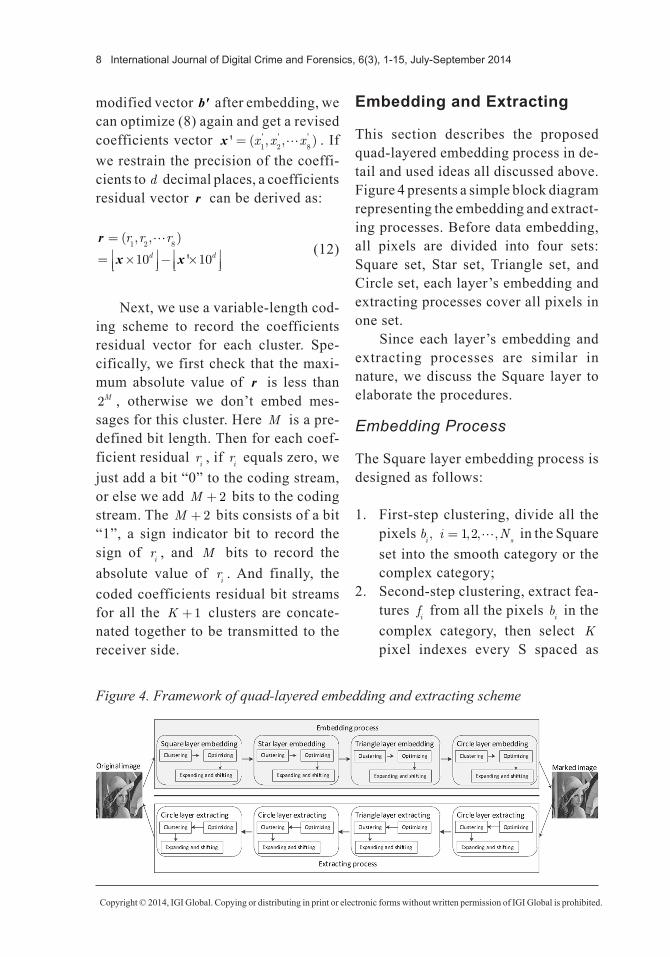
This section describes the proposed quad-layered embedding process in de-tail and used ideas all discussed above. Figure 4 presents a simple block diagram representing the embedding and extract-ing processes. Before data embedding, all pixels are divided into four sets: Square set, Star set, Triangle set, and Circle set, each layer’s embedding and extracting processes cover all pixels in one set.

Since each layer’s embedding and extracting processes are similar in nature, we discuss the Square layer to elaborate the procedures.

Embedding Process

The Square layer embedding process is designed as follows:

1. First-step clustering, divide all the pixels b i N

i s, , , , = 1 2� in the Square

set into the smooth category or the complex category;

2. Second-step clustering, extract fea-tures f

i from all the pixels b

i in the

complex category, then select K pixel indexes every S spaced as

Figure 4. Framework of quad-layered embedding and extracting scheme



initial cluster centroids to run the K-means algorithm on the features space to subdivide all complex cat-egory pixels into K clusters;

3. For k K= 0 : :a. Collect all pixels b j c c cj Nk, , , ,=

1 2� and predic-

tion context vectors aj to form

matrix A and vector b in (9);b. Estimate the optimal pixel

predictor coefficients x = ( , , )x x x

1 2 8� by solving (8),

and then calculate the corre-sponding prediction errors e

j

using (10);c. Embed messages into the predic-

tion errors ej using expanding

and shifting techniques de-scribed in (2), then calculate the coefficients residual vector r

k

by (12) and generate the coded residual bit stream r

sk as dis-

cussed in Section III-C;4. Finally, concatenate all the coded

residual bit streams rskk K, , , , = 0 1 2�

together and embedded them into the LSBs of some preserved pixels.

Extracting Process

The Square layer extracting process is designed as follows:

1. Extract all the coded residual bit streams r

skk K, , , , = 0 1 2� from the

LSBs of some preserved pixels;

2. First-step clustering, divide all the pixels b i N

i s, , , , = 1 2� in the Square

set into the smooth category or the complex category;

3. Second-step clustering, extract fea-tures f

i from all the pixels b

i in the

complex category, then select K pixel indexes every S spaced as initial cluster centroids run the K-means algorithm on the features space to subdivide all complex cat-egory pixels into K clusters;

4. For k K= 0 : :a. Collect all pixelsb j c c cj Nk

' , , , ,=1 2� and predic-

tion context vectors aj to form

matrix A and vector b ' in (9);b. Estimate the optimal pixel

predictor coefficients x ' ( , , )' ' '= x x x

1 2 8� by solving

(8), and together with the coded residual bit stream r

sk,

recover the original optimal pixel predictor coefficients x = ( , , )x x x

1 2 8� ;

c. Calculate prediction errors ej'

using (11), then extract messages using expanding and shifting techniques described in (3), at the same time recover the origi-nal prediction errors e

j;

d. Using the recovered prediction errors e

j, the original pixel val-

ues bj can be restored losslessly

through (10).



SIMULATIONS

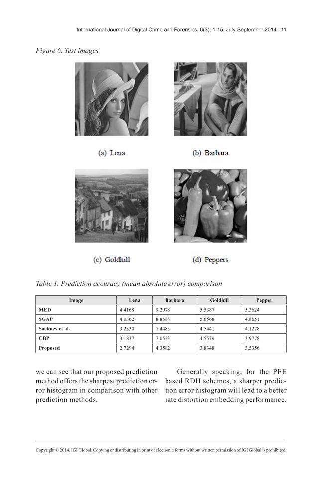
First, the proposed two-step clustering and optimizing scheme is compared to other four prediction methods consid-ered, namely, MED (Thodi & Rodriguez, 2007), Sachnev et al.’s method (2009), the simplified gradient-adjusted pre-dictor (SGAP) (Coltuc, 2011), and the checkerboard based prediction (CBP) (R.M, W, & Guo, 2014), using typical 512 × 512 gray scale images as shown in Figure 6. Table 1 records the comparison results of prediction accuracy in terms of MAE (mean absolute error), which is defined by:

MAEn

b bi i

i

n

= × −=∑1

1

ˆ (13)

Here for simplicity, we only process the Square set pixels for comparison, mean only a quarter of pixels are pre-dicted in the cover image. It can be observed from Table 1 that our cluster-ing and optimizing scheme provides the best prediction accuracy among all the competitors for all the four test images.

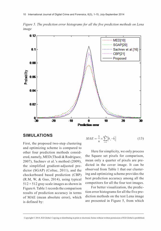
For better visualization, the predic-tion error histograms for all the five pre-diction methods on the test Lena image are presented in Figure 5, from which

Figure 5. The prediction error histograms for all the five prediction methods on Lena image



we can see that our proposed prediction method offers the sharpest prediction er-ror histogram in comparison with other prediction methods.

Generally speaking, for the PEE based RDH schemes, a sharper predic-tion error histogram will lead to a better rate distortion embedding performance.

Figure 6. Test images

Table 1. Prediction accuracy (mean absolute error) comparison

Image Lena Barbara Goldhill Pepper

MED 4.4168 9.2978 5.5387 5.3624

SGAP 4.0362 8.8888 5.6568 4.8651

Sachnev et al. 3.2330 7.4485 4.5441 4.1278

CBP 3.1837 7.0533 4.5579 3.9778

Proposed 2.7294 4.3582 3.8348 3.5356



By observing (2), we can see that the embedding capacity is determined by the total number of prediction errors falling in the interval [ , ]T T

n p, so the

sharper the prediction error histogram is, the higher the embedding capacity can be achieved. And vice versa, for a given embedding payload, the sharper the histogram, the less the number of pixels falling out the interval [ , ]T T

n p,

which will result in less shifting distor-tion.

For our proposed two-step clustering and optimizing scheme, the main weak-ness is the extra bits to record the coded residual bit streams r

skk K, , , , = 0 1 2�

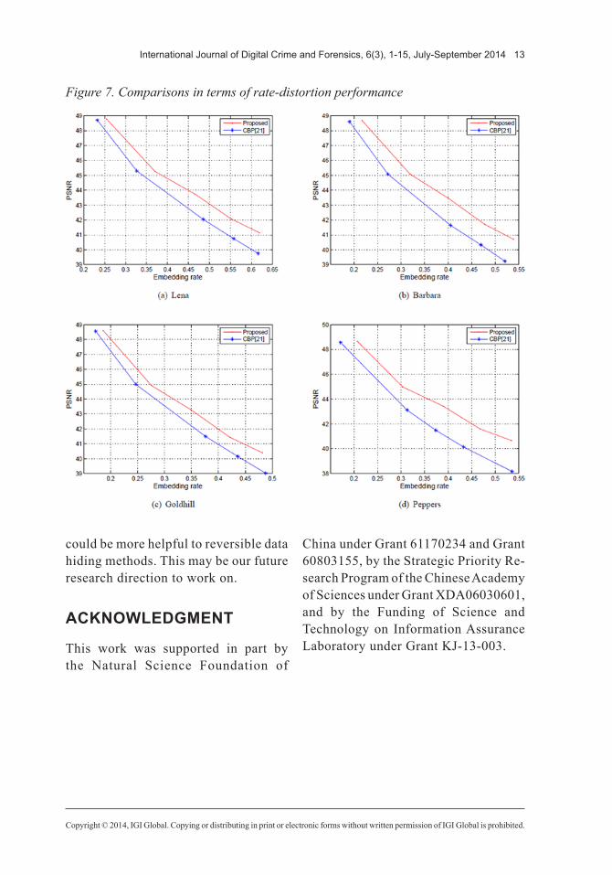
introduced in Section III-C. Next, to demonstrate that prediction accuracy directly influence the embedding per-formance of PEE based RDH methods. We compare our proposed quad-layered embedding scheme with the CBP meth-od (R.M et al., 2014) to process all the pixels in the cover image. Both predic-tion methods are combined with the PEE scheme in Section II to embed mes-sages. For our proposed scheme, the smooth threshold T

v is set to 25, the

cluster parameter K is set to 25, the decimal place parameter d and bit length parameter M in Section III-B are set with d = 2 and M = 3 . Embedding performance comparison results for various embedding rates are demon-strated by Figure 7.

Observing from Figure 7, for the Lena image and the Goldhill image, our proposed scheme earns 1.0dB higher PSNR than the CBP method (R.M et al., 2014) on average. And for the Barbara image and especially the Peppers image, the gains of PSNR increase to 2dB on average. As we can see in Figure 6, the Barbara image and the Peppers image exploit better structural self-similarities than the other two images, and this is why our clustering and optimizing scheme performs much better than the CBP method (R.M et al., 2014) method.

CONCLUSION

This paper presents a two-step clustering and optimizing pixel prediction method for prediction-error expansion (PEE) based reversible data hiding, which ex-ploits self-similarities and group struc-tural information of non-local image patches. And in order to traverse all the pixels in the cover image, a quad-layered embedding scheme is proposed accord-ingly. Compared to other fixed or con-tent adaptive pixel predictors that treat each pixel independently, our proposed method offers the best prediction ac-curacy. Experimental results imply that structural self-similarities of intra non-local image patches is a good property to benefit pixel prediction, so structural self-similarities across multiple images or even between a dataset of images



could be more helpful to reversible data hiding methods. This may be our future research direction to work on.

ACKNOWLEDGMENT

This work was supported in part by the Natural Science Foundation of

China under Grant 61170234 and Grant 60803155, by the Strategic Priority Re-search Program of the Chinese Academy of Sciences under Grant XDA06030601, and by the Funding of Science and Technology on Information Assurance Laboratory under Grant KJ-13-003.

Figure 7. Comparisons in terms of rate-distortion performance



REFERENCES

Bao, F., Deng, R. H., Ooi, B. C., & Yang, Y. (2005, December). Tailored reversible watermarking schemes for authentication of electronic clinical at-las. IEEE Transactions on Information Technology in Biomedicine, 9(4), 554–563. doi:10.1109/TITB.2005.855556 PMID:16379372

Caldelli, R., Filippini, F., & Becarelli, R. (2010, Jan). Reversible watermarking techniques: An overview and a classifi-cation. EURASIP J.Inf. Secur, 2010(2).

Chung, K., Huang, Y.-H., Chang, P.-C., & Liao, H.-Y. M. (2010, November). Reversible data hiding-based approach for intra-frame error concealment in H.264/AVC. IEEE Transactions on Circuits and Systems for Video Technol-ogy, 20(11), 1643–1647. doi:10.1109/TCSVT.2010.2077577

Coltuc, D. (2011, September). Improved embedding for prediction-based re-versible watermarking. IEEE Trans. Inf. Forens. Security, 6(3), 873–882. doi:10.1109/TIFS.2011.2145372

Fallahpour, M. (2008, October). Revers-ible image data hiding based on gradient adjusted prediction. IEICE Electronics Express, 5(20), 870–876. doi:10.1587/elex.5.870

Feng, J. et al. (2006, May). Reversible watermarking: Current status and key issues. International Journal of Network Security, 2(3), 161–171.

Fridrich, J., Goljan, M., & Du, R. (2002, January). Lossless data embedding for all image formats. Proceedings of the Soci-ety for Photo-Instrumentation Engineers, 4675, 572–583. doi:10.1117/12.465317

Hu, X., Zhang, W., Hu, X., Yu, N., Zhao, X., & Li, F. (2013, May). Fast Estimation of Optimal Marked-Signal Distribu-tion for Reversible Data Hiding. IEEE Trans. on Information Forensics and Security, 8(5), 779–788. doi:10.1109/TIFS.2013.2256131

Hu, X., Zhang, W., & Yu, N. (2014, June). Optimizing Pixel Predictors Based on Self-similarities for Reversible Data Hiding. Accepted by International Con-ference on Intelligent Information Hid-ing and Multimedia Signal Processing.

Li, X., Yang, B., & Zeng, T. (2011, December). Efficient reversible water-marking based on adaptive prediction-error expansion and pixel selection. IEEE Transactions on Image Process-ing, 20(12), 3524–3533. doi:10.1109/TIP.2011.2150233 PMID:21550888

Luo, L. et al. (2010, March). Reversible image watermarking using interpolation technique. IEEE Trans. Inf. Forensics Security, 5(1), 187–193. doi:10.1109/TIFS.2009.2035975

Ni, Z., Shi, Y., Ansari, N., & Wei, S. (2006, March). Reversible data hiding. IEEE Transactions on Circuits and Sys-tems for Video Technology, 16(3), 354–362. doi:10.1109/TCSVT.2006.869964

http://dx.doi.org/10.1109/TITB.2005.855556

http://www.ncbi.nlm.nih.gov/pubmed/16379372

http://dx.doi.org/10.1109/TCSVT.2010.2077577


http://dx.doi.org/10.1109/TIFS.2011.2145372

http://dx.doi.org/10.1587/elex.5.870

http://dx.doi.org/10.1587/elex.5.870

http://dx.doi.org/10.1117/12.465317



http://dx.doi.org/10.1109/TIP.2011.2150233








Ou, B., Li, X., Zhao, Y., & Ni, R. (2013, October). Reversible data hiding based on PDE predictor. Journal of Systems and Software, 86(10), 2700–2709. doi:10.1016/j.jss.2013.05.077

Peng, F., Li, X., & Yang, B. (2012, January). Adaptive reversible data hiding scheme based on integer trans-form. Signal Processing, 92(1), 54–62. doi:10.1016/j.sigpro.2011.06.006

Rad, R. M., KokSheik Wong, , & Jing-Ming Guo, R.M. (2014, April). A unified data embedding and scrambling method. IEEE Transactions on Image Process-ing, 23(4), 1463–1475. doi:10.1109/TIP.2014.2302681 PMID:24565789

Sachnev, V., Kim, H., Nam, J., Suresh, S., & Shi, Y. (2009, July). Reversible watermarking algorithm using sorting and prediction. IEEE Transactions on Circuits and Systems for Video Tech-nology, 19(7), 989–999. doi:10.1109/TCSVT.2009.2020257

Shi, Y. (2004). Reversible data hiding. Proc. IWDW (vol. 3304, pp. 1-12).

Shi, Y., Ni, Z., Zou, D., Liang, C., & Xuan, G. (2004, May). Lossless data hiding: fundamentals , algori thms and applications. Proc. IEEE ISCAS (vol. 2, pp. 33-36). doi:10.1109/IS-CAS.2004.1329201

Thodi, D., & Rodriguez, J. (2007, March). Expansion embedding tech-niques for reversible watermarking. IEEE Transactions on Image Process-ing, 16(3), 721–730. doi:10.1109/TIP.2006.891046 PMID:17357732

Tian, J. (2003, August). Reversible data embedding using a difference expansion. IEEE Transactions on Circuits and Sys-tems for Video Technology, 13(8), 890–896. doi:10.1109/TCSVT.2003.815962

Tsai, P., Hu, Y., & Yeh, H. (2009). Reversible image hiding scheme using predictive coding and histogram shifting. Signal Processing, 89(6), 1129–1143. doi:10.1016/j.sigpro.2008.12.017

Wang, C., Li, X., & Yang, B. (2010). Ef-ficient reversible image watermarking by using dynamical prediction-error expan-sion. Proc. IEEE ICIP (pp. 3673-3676).

Wu, H., & Huang, J. (2012, Decem-ber). Reversible image watermarking on prediction errors by efficient histo-gram modification. Signal Processing, 92(12), 3000–3009. doi:10.1016/j.sigpro.2012.05.034

Yang, W., Chung, K., Liao, H., & Yu, W. (2013, February). Efficient reversible data hiding algorithm based on gradient-based edge direction prediction. Journal of Systems and Software, 86(2), 567–580. doi:10.1016/j.jss.2012.09.041

Zhang, W., Hu, X., Li, X., & Yu, N. (2013, July). Recursive Histogram Modifica-tion: Establishing Equivalency between Reversible Data Hiding and Lossless Data Compression. IEEE Transactions on Image Processing, 22(7), 2775–2785. doi:10.1109/TIP.2013.2257814 PMID:23591495

http://dx.doi.org/10.1016/j.jss.2013.05.077

http://dx.doi.org/10.1016/j.sigpro.2011.06.006






http://dx.doi.org/10.1109/ISCAS.2004.1329201

http://dx.doi.org/10.1109/ISCAS.2004.1329201








http://dx.doi.org/10.1016/j.jss.2012.09.041



Documents

Optimizing Non-Local Pixel Predictors for Reversible …staff.ustc.edu.cn/~zhangwm/Paper/2014_3.pdfPixel Predictors for Reversible Data Hiding ... of the differences ... be saved for