Optimization Techniques

M. Fatih Amasyalı

Steepest Descent

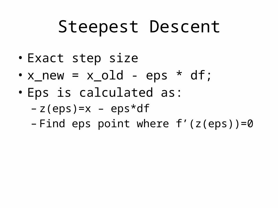
• Exact step size• x_new = x_old - eps * df; • Eps is calculated as:

– z(eps)=x – eps*df– Find eps point where f’(z(eps))=0

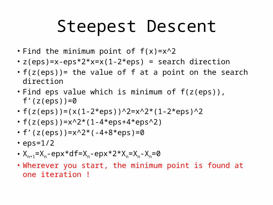
Steepest Descent• Find the minimum point of f(x)=x^2• z(eps)=x-eps*2*x=x(1-2*eps) = search direction• f(z(eps))= the value of f at a point on the search direction• Find eps value which is minimum of f(z(eps)), f’(z(eps))=0• f(z(eps))=(x(1-2*eps))^2=x^2*(1-2*eps)^2• f(z(eps))=x^2*(1-4*eps+4*eps^2)• f’(z(eps))=x^2*(-4+8*eps)=0 • eps=1/2• Xn+1=Xn-epx*df=Xn-epx*2*Xn=Xn-Xn=0• Wherever you start, the minimum point is found at one

iteration !

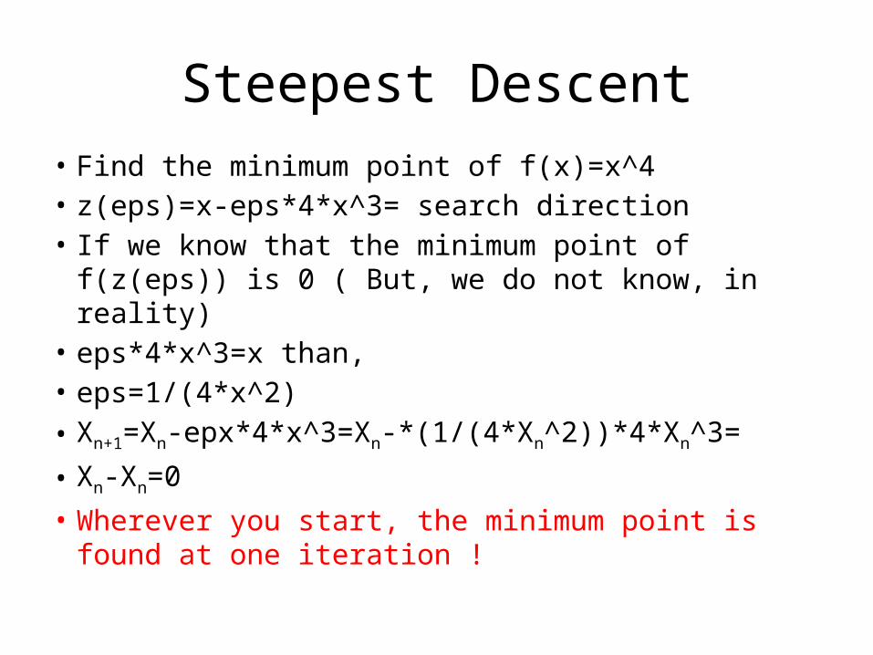
Steepest Descent• Find the minimum point of f(x)=x^4• z(eps)=x-eps*4*x^3= search direction• If we know that the minimum point of f(z(eps)) is 0 ( But,

we do not know, in reality)• eps*4*x^3=x than,• eps=1/(4*x^2)• Xn+1=Xn-epx*4*x^3=Xn-*(1/(4*Xn^2))*4*Xn^3=

• Xn-Xn=0• Wherever you start, the minimum point is found at one

iteration !

Steepest Descent in 2 dims.

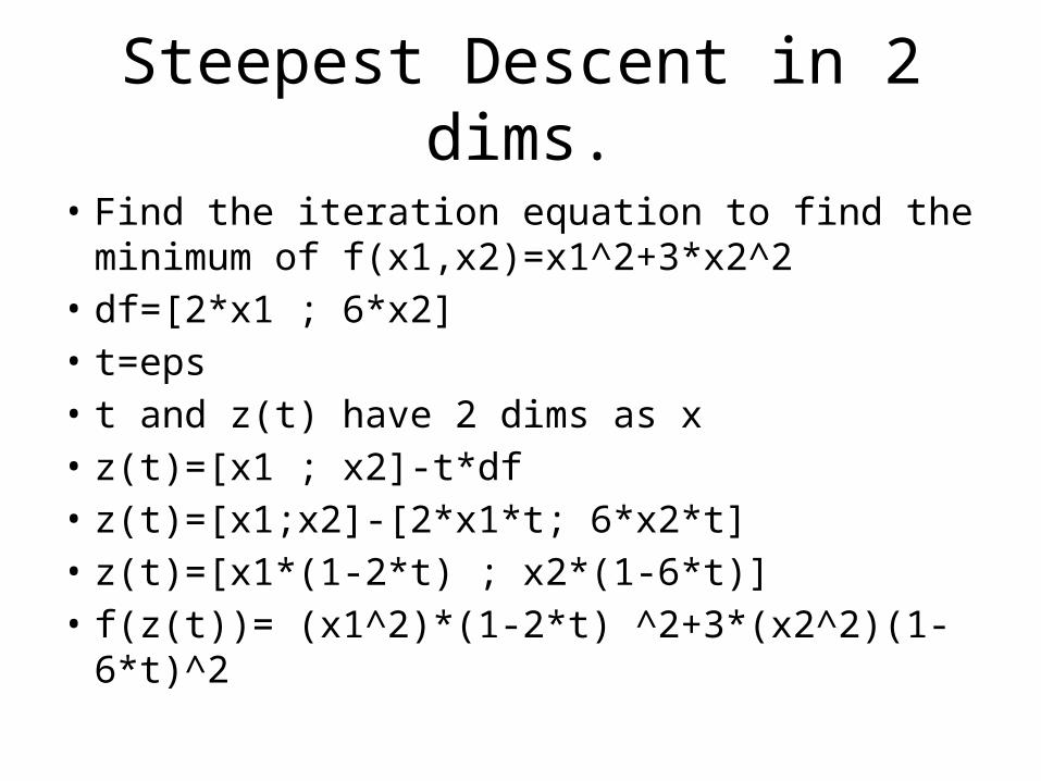
• Find the iteration equation to find the minimum of f(x1,x2)=x1^2+3*x2^2

• df=[2*x1 ; 6*x2]• t=eps • t and z(t) have 2 dims as x• z(t)=[x1 ; x2]-t*df• z(t)=[x1;x2]-[2*x1*t; 6*x2*t]• z(t)=[x1*(1-2*t) ; x2*(1-6*t)]• f(z(t))= (x1^2)*(1-2*t) ^2+3*(x2^2)(1-6*t)^2

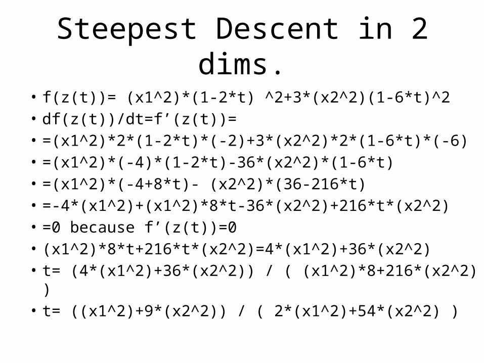
Steepest Descent in 2 dims.

• f(z(t))= (x1^2)*(1-2*t) ^2+3*(x2^2)(1-6*t)^2• df(z(t))/dt=f’(z(t))=• =(x1^2)*2*(1-2*t)*(-2)+3*(x2^2)*2*(1-6*t)*(-6)• =(x1^2)*(-4)*(1-2*t)-36*(x2^2)*(1-6*t)• =(x1^2)*(-4+8*t)- (x2^2)*(36-216*t)• =-4*(x1^2)+(x1^2)*8*t-36*(x2^2)+216*t*(x2^2)• =0 because f’(z(t))=0• (x1^2)*8*t+216*t*(x2^2)=4*(x1^2)+36*(x2^2)• t= (4*(x1^2)+36*(x2^2)) / ( (x1^2)*8+216*(x2^2) )• t= ((x1^2)+9*(x2^2)) / ( 2*(x1^2)+54*(x2^2) )

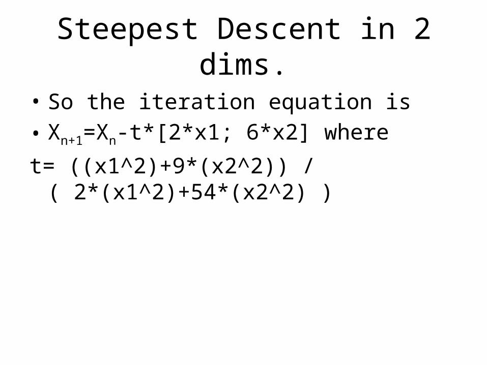
Steepest Descent in 2 dims.

• So the iteration equation is • Xn+1=Xn-t*[2*x1; 6*x2] where

t= ((x1^2)+9*(x2^2)) / ( 2*(x1^2)+54*(x2^2) )

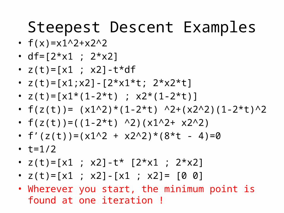
Steepest Descent Examples• f(x)=x1^2+x2^2• df=[2*x1 ; 2*x2]• z(t)=[x1 ; x2]-t*df• z(t)=[x1;x2]-[2*x1*t; 2*x2*t]• z(t)=[x1*(1-2*t) ; x2*(1-2*t)]• f(z(t))= (x1^2)*(1-2*t) ^2+(x2^2)(1-2*t)^2• f(z(t))=((1-2*t) ^2)(x1^2+ x2^2)• f’(z(t))=(x1^2 + x2^2)*(8*t - 4)=0• t=1/2• z(t)=[x1 ; x2]-t* [2*x1 ; 2*x2]• z(t)=[x1 ; x2]-[x1 ; x2]= [0 0]• Wherever you start, the minimum point is found at one

iteration !

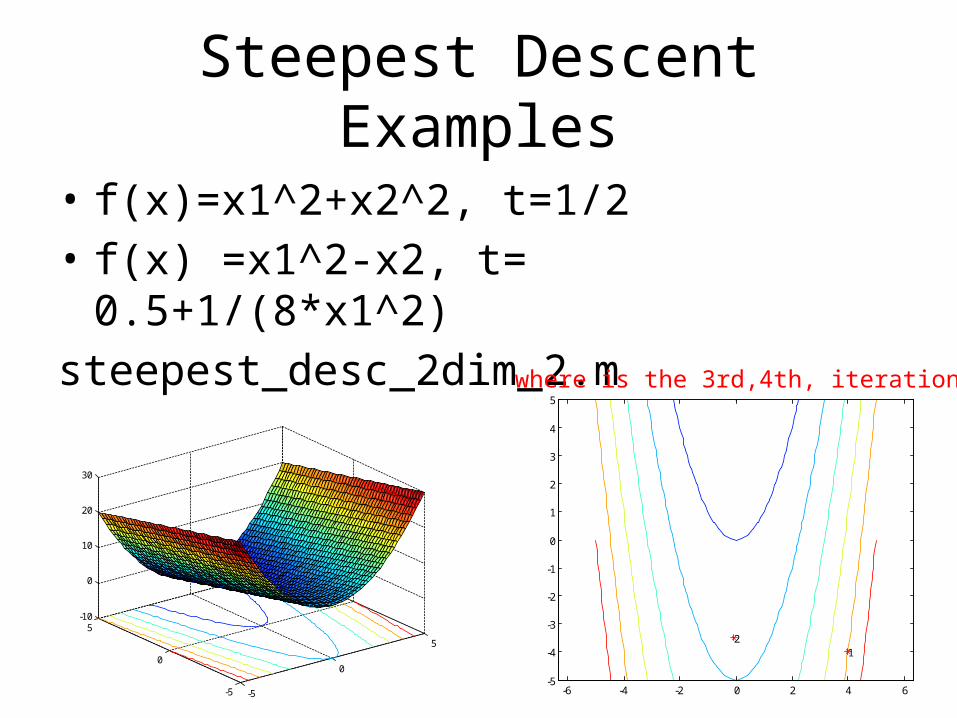
Steepest Descent Examples

• f(x)=x1^2+x2^2, t=1/2• f(x) =x1^2-x2, t= 0.5+1/(8*x1^2) steepest_desc_2dim_2.m

-5

0

5

-5

0

5-10

0

10

20

30

12

-6 -4 -2 0 2 4 6-5

-4

-3

-2

-1

0

1

2

3

4

5

where is the 3rd,4th, iterations…?

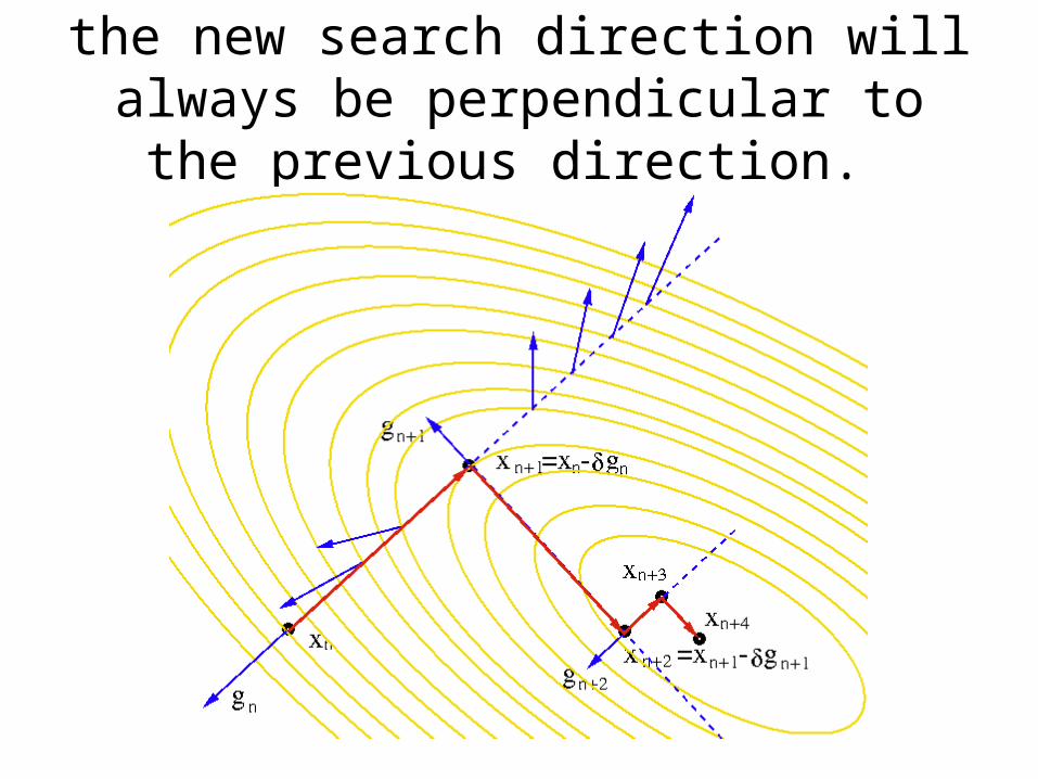
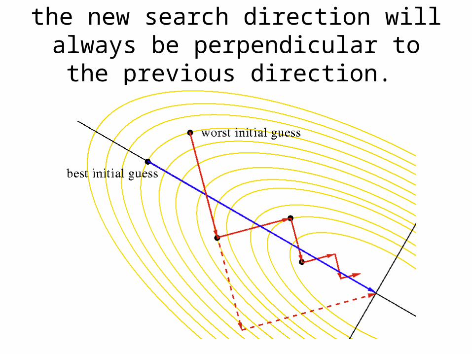
the new search direction will always be perpendicular to the previous direction.

the new search direction will always be perpendicular to the previous direction.

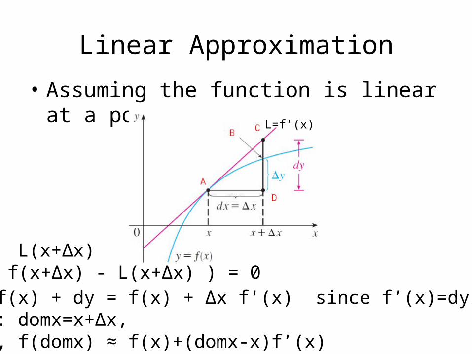
Linear Approximation

• Assuming the function is linear at a point.L=f’(x)

f(x+Δx) ≈ L(x+Δx) lim (Δx0) ( f(x+Δx) - L(x+Δx) ) = 0L(x+Δx) =f(x) + dy = f(x) + Δx f'(x) since f’(x)=dy/dxNew point: domx=x+Δx, Δx=domx-x, f(domx) ≈ f(x)+(domx-x)f’(x)

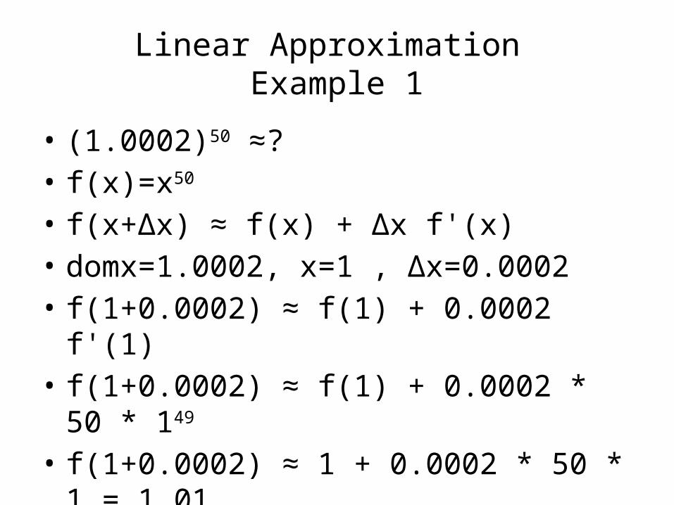
Linear Approximation Example 1

• (1.0002)50 ≈?• f(x)=x50

• f(x+Δx) ≈ f(x) + Δx f'(x)• domx=1.0002, x=1 , Δx=0.0002• f(1+0.0002) ≈ f(1) + 0.0002 f'(1)• f(1+0.0002) ≈ f(1) + 0.0002 * 50 * 149

• f(1+0.0002) ≈ 1 + 0.0002 * 50 * 1 = 1.01

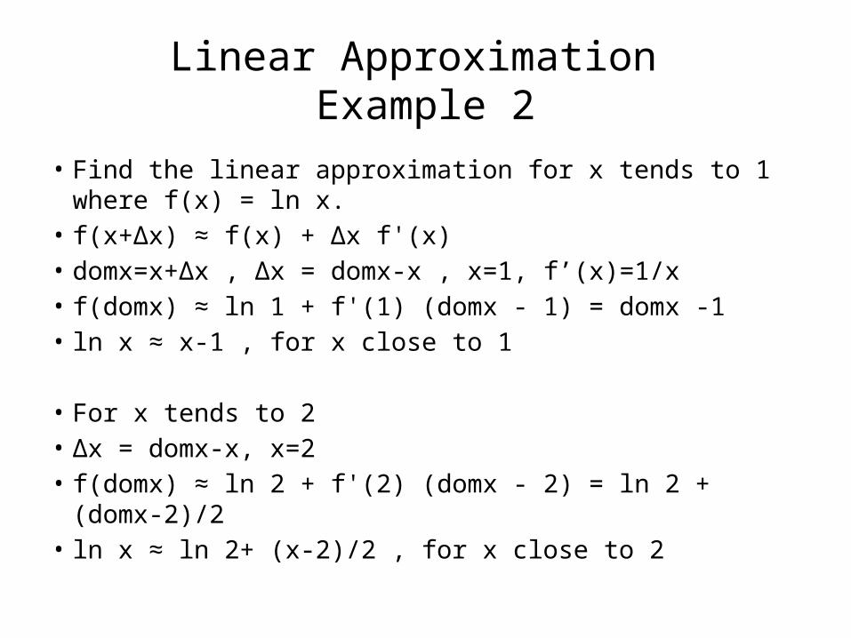
Linear Approximation Example 2

• Find the linear approximation for x tends to 1 where f(x) = ln x.• f(x+Δx) ≈ f(x) + Δx f'(x)• domx=x+Δx , Δx = domx-x , x=1, f’(x)=1/x• f(domx) ≈ ln 1 + f'(1) (domx - 1) = domx -1• ln x ≈ x-1 , for x close to 1

• For x tends to 2• Δx = domx-x, x=2• f(domx) ≈ ln 2 + f'(2) (domx - 2) = ln 2 + (domx-2)/2• ln x ≈ ln 2+ (x-2)/2 , for x close to 2

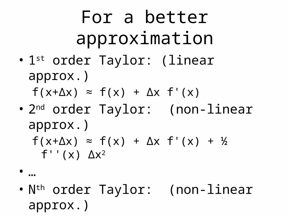
For a better approximation

• 1st order Taylor: (linear approx.)f(x+Δx) ≈ f(x) + Δx f'(x)

• 2nd order Taylor: (non-linear approx.)f(x+Δx) ≈ f(x) + Δx f'(x) + ½ f''(x) Δx2

• …• Nth order Taylor: (non-linear approx.)• f(x+Δx) ≈ ∑ (f (i)’(x) Δxi )/ i! i=0…N

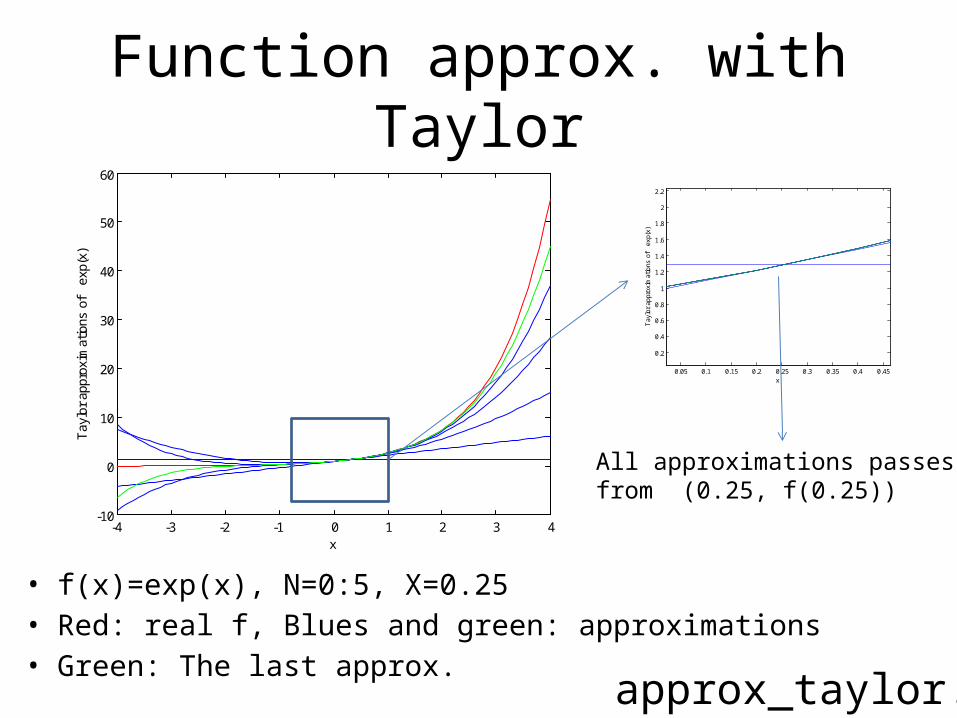
Function approx. with Taylor

• f(x)=exp(x), N=0:5, X=0.25• Red: real f, Blues and green: approximations• Green: The last approx. approx_taylor.m

-4 -3 -2 -1 0 1 2 3 4-10

0

10

20

30

40

50

60

x

Tay

lor

appr

oxim

atio

ns o

f

exp(

x)

0.05 0.1 0.15 0.2 0.25 0.3 0.35 0.4 0.45

0.2

0.4

0.6

0.8

1

1.2

1.4

1.6

1.8

2

2.2

x

Tay

lor

appr

oxim

atio

ns o

f

exp(

x)

All approximations passes from (0.25, f(0.25))

-4 -3 -2 -1 0 1 2 3 4-60

-40

-20

0

20

40

60

x

Tay

lor

appr

oxim

atio

ns o

f

exp(

x)

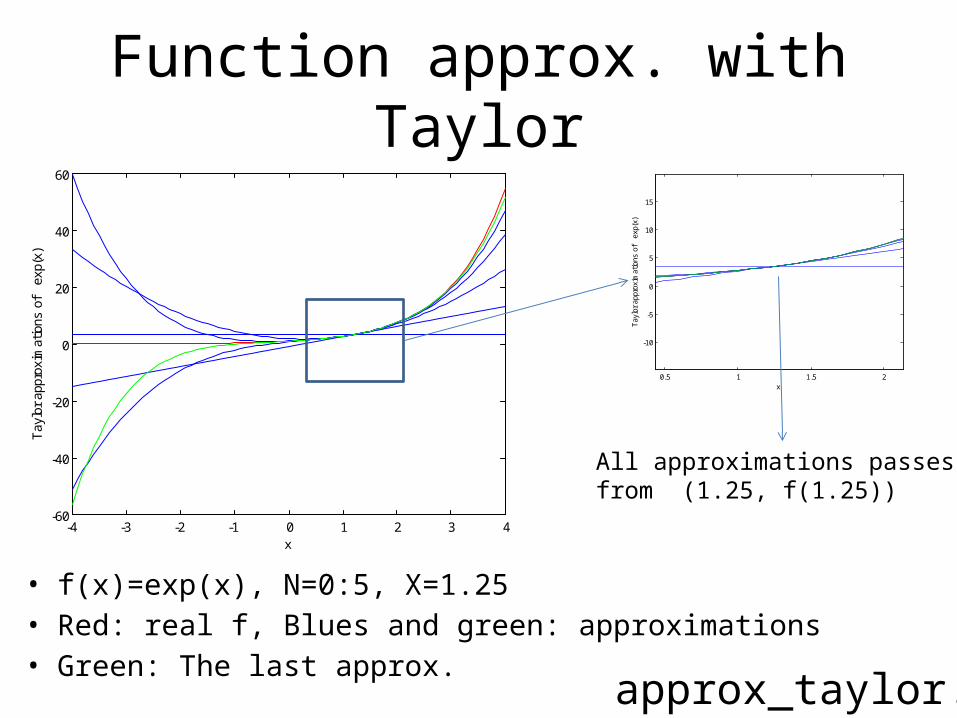
Function approx. with Taylor

• f(x)=exp(x), N=0:5, X=1.25• Red: real f, Blues and green: approximations• Green: The last approx. approx_taylor.m

All approximations passes from (1.25, f(1.25))

0.5 1 1.5 2

-10

-5

0

5

10

15

x

Tay

lor

appr

oxim

atio

ns o

f

exp(

x)

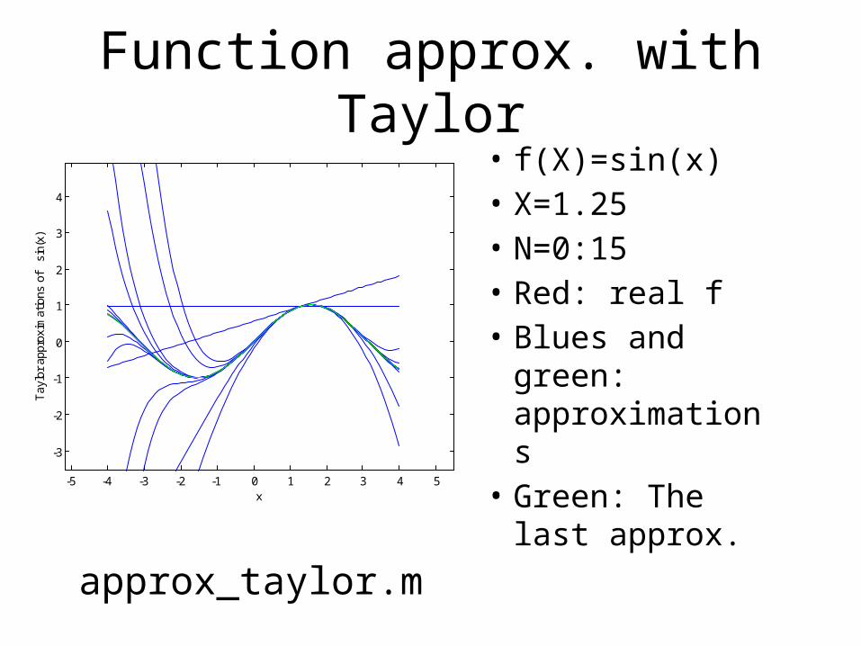
Function approx. with Taylor• f(X)=sin(x)• X=1.25• N=0:15• Red: real f• Blues and green:

approximations• Green: The last

approx.

approx_taylor.m

-5 -4 -3 -2 -1 0 1 2 3 4 5

-3

-2

-1

0

1

2

3

4

x

Tay

lor

appr

oxim

atio

ns o

f

sin(

x)

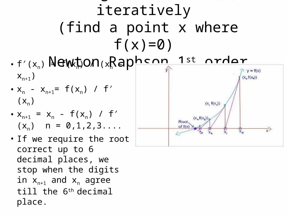
Finding a root of f(x) iteratively (find a point x where f(x)=0) Newton Raphson 1st order

• f (x′ n) = f(xn) / (xn - xn+1)

• xn - xn+1= f(xn) / f (x′ n)

• xn+1 = xn - f(xn) / f (x′ n) n = 0,1,2,3....

• If we require the root correct up to 6 decimal places, we stop when the digits in xn+1 and xn agree till the 6th

decimal place.

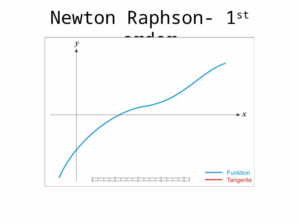
Newton Raphson- 1st order

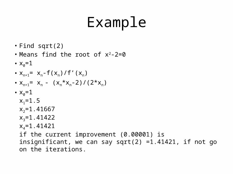
Example• Find sqrt(2)• Means find the root of x2-2=0• x0=1

• xn+1= xn-f(xn)/f’(xn)

• xn+1= xn - (xn*xn-2)/(2*xn)

• x0=1 x1=1.5 x2=1.41667x3=1.41422x4=1.41421if the current improvement (0.00001) is insignificant, we can say sqrt(2) =1.41421, if not go on the iterations.

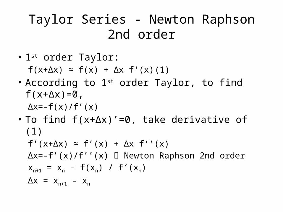
Taylor Series - Newton Raphson 2nd order

• 1st order Taylor: f(x+Δx) ≈ f(x) + Δx f'(x) (1)

• According to 1st order Taylor, to find f(x+Δx)=0, Δx=-f(x)/f’(x)

• To find f(x+Δx)’=0, take derivative of (1) f'(x+Δx) ≈ f’(x) + Δx f‘’(x)Δx=-f’(x)/f’’(x) Newton Raphson 2nd orderxn+1 = xn - f(xn) / f (x′ n)

Δx = xn+1 - xn

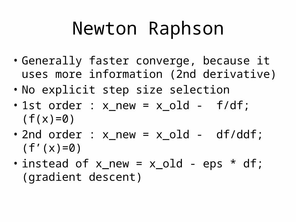
Newton Raphson

• Generally faster converge, because it uses more information (2nd derivative)

• No explicit step size selection • 1st order : x_new = x_old - f/df; (f(x)=0)• 2nd order : x_new = x_old - df/ddf; (f’(x)=0) • instead of x_new = x_old - eps * df; (gradient

descent)

-2 -1 0 1 2 3 4-10

0

10

20

30

40

50

60

70

1

2

3456789101112131415161718192021222324252627282930313233343536373839404142434445464748495051525354555657585960616263646566676869707172737475767778798081828384858687888990919293949596979899100101102103104105106107108109110111112113114115116117118119120121122123124125126127128129130131132133134135136137138139140141142143144145146147148149150151152153154155156157158159160161162163164165166167168169170171172173174175176177178179180181182183184185186187188189190191192193194195196197198199200

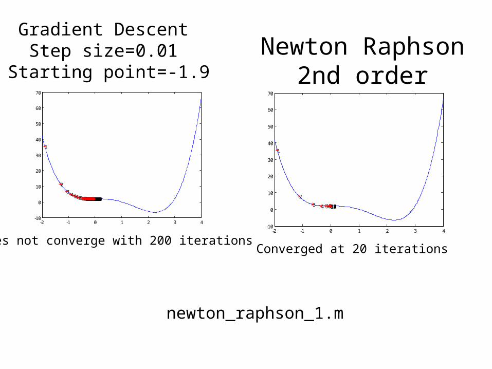
Gradient Descent Step size=0.01

Starting point=-1.9

-2 -1 0 1 2 3 4-10

0

10

20

30

40

50

60

70

1

2

3 4 5678910111213141516171819

Does not converge with 200 iterationsConverged at 20 iterations

Newton Raphson 2nd order

newton_raphson_1.m

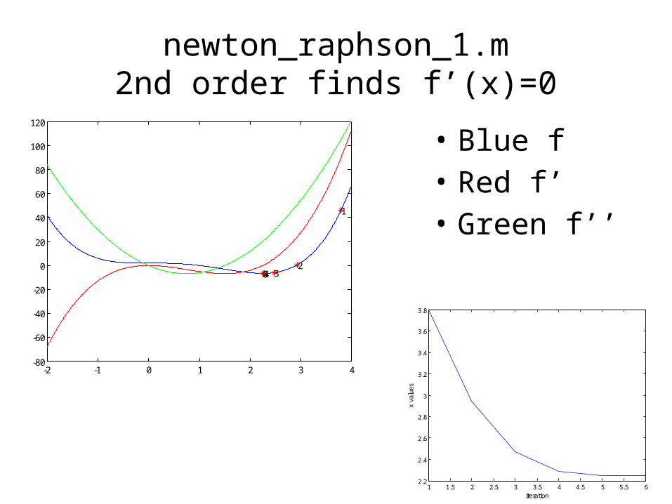
newton_raphson_1.m2nd order finds f’(x)=0

• Blue f• Red f’• Green f’’

-2 -1 0 1 2 3 4-80

-60

-40

-20

0

20

40

60

80

100

120

1

23456

1 1.5 2 2.5 3 3.5 4 4.5 5 5.5 62.2

2.4

2.6

2.8

3

3.2

3.4

3.6

3.8

iteration

x va

lues

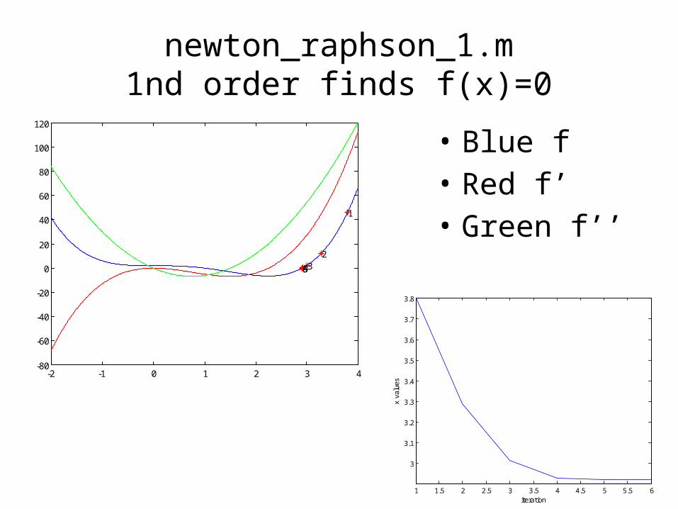
newton_raphson_1.m1nd order finds f(x)=0

• Blue f• Red f’• Green f’’

-2 -1 0 1 2 3 4-80

-60

-40

-20

0

20

40

60

80

100

120

1

23456

1 1.5 2 2.5 3 3.5 4 4.5 5 5.5 6

3

3.1

3.2

3.3

3.4

3.5

3.6

3.7

3.8

iteration

x va

lues

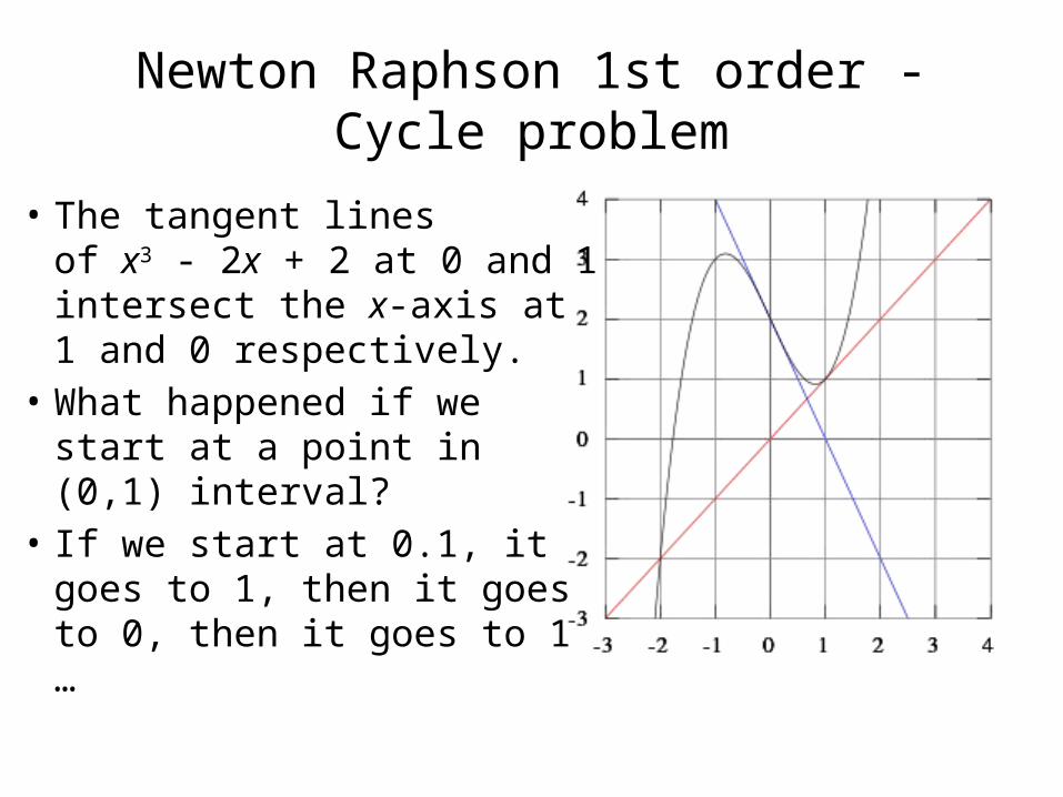
Newton Raphson 1st order -Cycle problem

• The tangent lines of x3 - 2x + 2 at 0 and 1 intersect the x-axis at 1 and 0 respectively.

• What happened if we start at a point in (0,1) interval?

• If we start at 0.1, it goes to 1, then it goes to 0, then it goes to 1 …

Newton Raphson

• Faster convergence (lower iteration number)• But, more calculation for each iteration

References • http://math.tutorvista.com/calculus/newton-raphson-method.html • http://math.tutorvista.com/calculus/linear-approximation.html • http://en.wikipedia.org/wiki/Newton's_method • http://en.wikipedia.org/wiki/Steepest_descent • http://www.pitt.edu/~nak54/Unconstrained_Optimization_KN.pdf • http://mathworld.wolfram.com/MatrixInverse.html • http://lpsa.swarthmore.edu/BackGround/RevMat/MatrixReview.html • http://www.cut-the-knot.org/arithmetic/algebra/Determinant.shtml • Matematik Dünyası, MD 2014-II, Determinantlar• http://www.sharetechnote.com/html/EngMath_Matrix_Main.html • Advanced Engineering Mathematics , Erwin Kreyszig, 10th Edition, John Wiley & Sons, 2011• http://en.wikipedia.org/wiki/Finite_difference • http://ocw.usu.edu/Civil_and_Environmental_Engineering/Numerical_Methods_in_Civil_Engine

ering/NonLinearEquationsMatlab.pdf• http://www-math.mit.edu/~djk/calculus_beginners/chapter09/section02.html • http://stanford.edu/class/ee364a/lectures/intro.pdf • http://fourier.eng.hmc.edu/e176/lectures/NM/node28.html