Embed Size (px)
Citation preview

A350 Take-off Configuration Optimization using aSurrogate-based Steepest Descent Method
Miguel Afonso Rita
Thesis to obtain the Master of Science Degree in
Aerospace Engineering
Supervisors: Prof. Fernando José Parracho LauDr. Julien Delbove
Examination Committee
Chairperson: Prof. Filipe Szolnoky Ramos Pinto CunhaSupervisor: Prof. Fernando José Parracho LauMember of the Committee: Dr. José Lobo do Vale
November 2014

ii

For my family, unconditionally there, always.
iii

iv

Acknowledgments
First and foremost, I would like to express my gratitude to my internship tutor at Airbus, Mr. Julien Del-
bove, for his constant support, expertise and commitment. His overall guidance and trust were what
made it all possible.
I would also like to address a big thank you to Professor Fernando Lau and Professor Jose Vale for
their efforts, feedback and help in preparing this thesis for presentation here in Portugal.
Additionally, a deep thank you in general to the Instituto Superior Tecnico, Sup’Aero and Airbus, namely
to all the teachers and staff who work in these places, and who empower students to take challenges
akin to this one.
Last but certainly not least, here’s to my pals Cardeira, Brinco and Clemente. For your friendship, I
can only be grateful.
v

vi

Resumo
Actualmente, a determinacao de configuracoes de descolagem optimas de uma aeronave e feita recor-
rendo a extensas campanhas de ensaios em voo, com um elevado custo monetario associado. Este
custo limita frequentemente nao so a qualidade dos resultados obtidos, mas tambem o numero de
parametros que sao optimizados. O presente trabalho visa a implementacao de um algoritmo de
optimizacao inovador, baseado no metodo do gradiente, que permita determinar configuracoes optimas
de descolagem de uma maneira sistematica, economica e extensıvel. Para alcancar estes objectivos,
o algoritmo recorre a modelos substitutos e planos de experiencia optimos. Os resultados obtidos
mostram que e de facto possıvel atingir optimos de uma maneira muito mais economica que no pas-
sado, desde que a modelacao dos dados seja feita cuidadosamente. Uma nova funcao objectivo es-
tatıstica baseada num metodo de propagacao de incerteza foi tambem implementada, com resultados
que vem suportar o que foi feito ate entao na industria. Para concluir, o trabalho desenvolvido demon-
strou nao so a aplicabilidade do metodo, mas tambem a sua extensibilidade a problemas diferentes ou
de diferentes dimensionalidades, abrindo as portas a poupancas de tempo e ganhos monetarios muito
significativos nas futuras campanhas de configuracao optima.
Palavras-chave: Performance aviao, Configuracao de descolagem, Optimizacao baseada
em modelos, Plano de experiencia, Metodo do gradiente.
vii

viii

Abstract
At present, determination of optimal aircraft takeoff configurations is done resorting to very expensive
and time-consuming flight testing. This often limits not only the quality of the optima found but also
the number of configuration parameters that can be optimized. The present work implements a novel
gradient steepest descent optimization algorithm to tackle this problem in an economically viable way.
To achieve this, it resorts to surrogate modelling and optimal design of experiment techniques, allowing
for flexibility and optimal information gain in process, respectively. Results obtained show satisfactory
accuracy as long as great care is taken in the modelling and interpolation of data. An innovative statistical
assessment of configuration optimality solidly supports the optima obtained thus far in the industry. This
work confirms the applicability of method for real-time flight testing and, more importantly, its scalability
and adaptability to different configuration problems or problem dimensionality, opening up the door for
potentially large savings in future optimal configuration campaigns.
Keywords: Aircraft Performance, Takeoff configuration, Surrogate-based optimization, Design
of experiment, Gradient steepest descent.
ix

x

Contents
Acknowledgments . . . . . . . . . . . . . . . . . . . . . . . . . . . . . . . . . . . . . . . . . . . v
Resumo . . . . . . . . . . . . . . . . . . . . . . . . . . . . . . . . . . . . . . . . . . . . . . . . . vii
Abstract . . . . . . . . . . . . . . . . . . . . . . . . . . . . . . . . . . . . . . . . . . . . . . . . . ix
List of Tables . . . . . . . . . . . . . . . . . . . . . . . . . . . . . . . . . . . . . . . . . . . . . . xiii
List of Figures . . . . . . . . . . . . . . . . . . . . . . . . . . . . . . . . . . . . . . . . . . . . . xvi
Nomenclature . . . . . . . . . . . . . . . . . . . . . . . . . . . . . . . . . . . . . . . . . . . . . . xvii
Abbreviations . . . . . . . . . . . . . . . . . . . . . . . . . . . . . . . . . . . . . . . . . . . . . . xix
1 Introduction 1
1.1 Context and motivation . . . . . . . . . . . . . . . . . . . . . . . . . . . . . . . . . . . . . . 1
1.2 Problem statement . . . . . . . . . . . . . . . . . . . . . . . . . . . . . . . . . . . . . . . . 2
1.3 Possible solutions . . . . . . . . . . . . . . . . . . . . . . . . . . . . . . . . . . . . . . . . 2
1.4 Thesis outline . . . . . . . . . . . . . . . . . . . . . . . . . . . . . . . . . . . . . . . . . . . 3
2 Aircraft Takeoff Optimization 4
2.1 Overview . . . . . . . . . . . . . . . . . . . . . . . . . . . . . . . . . . . . . . . . . . . . . 4
2.2 Takeoff Configurations . . . . . . . . . . . . . . . . . . . . . . . . . . . . . . . . . . . . . . 5
2.3 Air conditioning . . . . . . . . . . . . . . . . . . . . . . . . . . . . . . . . . . . . . . . . . . 5
2.4 Takeoff Speed Optimization . . . . . . . . . . . . . . . . . . . . . . . . . . . . . . . . . . . 5
2.4.1 Speed Ratios . . . . . . . . . . . . . . . . . . . . . . . . . . . . . . . . . . . . . . . 5
2.4.2 V1/VR Ratio Influence . . . . . . . . . . . . . . . . . . . . . . . . . . . . . . . . . . 6
2.4.3 V2/VS Ratio Influence . . . . . . . . . . . . . . . . . . . . . . . . . . . . . . . . . . 7
2.5 Optimization Process & Results . . . . . . . . . . . . . . . . . . . . . . . . . . . . . . . . . 8
3 Surrogate Modelling 10
3.1 Overview . . . . . . . . . . . . . . . . . . . . . . . . . . . . . . . . . . . . . . . . . . . . . 10
3.2 Techniques . . . . . . . . . . . . . . . . . . . . . . . . . . . . . . . . . . . . . . . . . . . . 11
3.2.1 Linear regression . . . . . . . . . . . . . . . . . . . . . . . . . . . . . . . . . . . . . 11
3.2.2 Response Surface Model . . . . . . . . . . . . . . . . . . . . . . . . . . . . . . . . 12
3.2.3 Gaussian Processes . . . . . . . . . . . . . . . . . . . . . . . . . . . . . . . . . . . 13
3.2.4 Splines in tension . . . . . . . . . . . . . . . . . . . . . . . . . . . . . . . . . . . . 14
xi

4 Design of Experiment 16
4.1 Overview . . . . . . . . . . . . . . . . . . . . . . . . . . . . . . . . . . . . . . . . . . . . . 16
4.2 General DoE Techniques . . . . . . . . . . . . . . . . . . . . . . . . . . . . . . . . . . . . 17
4.3 Optimal DoE Techniques . . . . . . . . . . . . . . . . . . . . . . . . . . . . . . . . . . . . 19
5 Uncertainty Propagation 21
5.1 Overview . . . . . . . . . . . . . . . . . . . . . . . . . . . . . . . . . . . . . . . . . . . . . 21
5.2 Techniques . . . . . . . . . . . . . . . . . . . . . . . . . . . . . . . . . . . . . . . . . . . . 21
5.2.1 Taylor Moment Propagation . . . . . . . . . . . . . . . . . . . . . . . . . . . . . . . 22
5.2.2 Gaussian Quadrature . . . . . . . . . . . . . . . . . . . . . . . . . . . . . . . . . . 22
5.2.3 Monte Carlo Methods . . . . . . . . . . . . . . . . . . . . . . . . . . . . . . . . . . 22
5.2.4 Univariate Reduced Quadrature . . . . . . . . . . . . . . . . . . . . . . . . . . . . 23
6 Optimal Configuration Search 25
6.1 Core Tools . . . . . . . . . . . . . . . . . . . . . . . . . . . . . . . . . . . . . . . . . . . . 25
6.1.1 OCTOPUS . . . . . . . . . . . . . . . . . . . . . . . . . . . . . . . . . . . . . . . . 25
6.1.2 OPTIMA . . . . . . . . . . . . . . . . . . . . . . . . . . . . . . . . . . . . . . . . . . 26
6.1.3 MACROS . . . . . . . . . . . . . . . . . . . . . . . . . . . . . . . . . . . . . . . . . 27
6.2 Overall Architecture . . . . . . . . . . . . . . . . . . . . . . . . . . . . . . . . . . . . . . . 27
6.2.1 Gradient Descent Rationale . . . . . . . . . . . . . . . . . . . . . . . . . . . . . . . 27
6.2.2 Algorithm Description . . . . . . . . . . . . . . . . . . . . . . . . . . . . . . . . . . 28
6.3 Implementation . . . . . . . . . . . . . . . . . . . . . . . . . . . . . . . . . . . . . . . . . . 35
6.3.1 DoE Generator . . . . . . . . . . . . . . . . . . . . . . . . . . . . . . . . . . . . . . 35
6.3.2 FT Simulator . . . . . . . . . . . . . . . . . . . . . . . . . . . . . . . . . . . . . . . 36
6.3.3 Objective Calculator . . . . . . . . . . . . . . . . . . . . . . . . . . . . . . . . . . . 39
6.3.4 Gradient Calculator . . . . . . . . . . . . . . . . . . . . . . . . . . . . . . . . . . . 48
6.3.5 Line Designer . . . . . . . . . . . . . . . . . . . . . . . . . . . . . . . . . . . . . . . 49
6.3.6 Line Builder . . . . . . . . . . . . . . . . . . . . . . . . . . . . . . . . . . . . . . . . 50
6.3.7 Line Optimizer . . . . . . . . . . . . . . . . . . . . . . . . . . . . . . . . . . . . . . 50
7 Results 51
7.1 Overview . . . . . . . . . . . . . . . . . . . . . . . . . . . . . . . . . . . . . . . . . . . . . 51
7.2 Single MTOW, Fixed Runway . . . . . . . . . . . . . . . . . . . . . . . . . . . . . . . . . . 51
7.3 Optimal Configuration, Fixed Runway . . . . . . . . . . . . . . . . . . . . . . . . . . . . . 54
7.4 Different OC, Varying Runway . . . . . . . . . . . . . . . . . . . . . . . . . . . . . . . . . . 67
7.5 Statistically Optimal Configuration . . . . . . . . . . . . . . . . . . . . . . . . . . . . . . . 71
8 Conclusion 72
Bibliography 78
xii

List of Tables
2.1 TO Parameters Categorization . . . . . . . . . . . . . . . . . . . . . . . . . . . . . . . . . 4
2.2 Fixed parameters for V1/VR study . . . . . . . . . . . . . . . . . . . . . . . . . . . . . . . 7
3.1 Different RSM types . . . . . . . . . . . . . . . . . . . . . . . . . . . . . . . . . . . . . . . 12
6.1 CoH steps - module correspondence. . . . . . . . . . . . . . . . . . . . . . . . . . . . . . 35
6.2 FT source data . . . . . . . . . . . . . . . . . . . . . . . . . . . . . . . . . . . . . . . . . . 37
7.1 Optimal Configuration for RL 4000m . . . . . . . . . . . . . . . . . . . . . . . . . . . . . . 54
7.2 3 Configuration Sets, Traditional and Optimal (∗) . . . . . . . . . . . . . . . . . . . . . . . 67
7.3 Different TO network coverage. . . . . . . . . . . . . . . . . . . . . . . . . . . . . . . . . . 70
7.4 Statistical OC results and their standard counterparts. . . . . . . . . . . . . . . . . . . . . 71
xiii

xiv

List of Figures
2.1 V1/VR MTOW limitations. . . . . . . . . . . . . . . . . . . . . . . . . . . . . . . . . . . . . 8
4.1 Optimal and non-optimal latin hypercubes . . . . . . . . . . . . . . . . . . . . . . . . . . . 18
6.1 CoH algorithm basic workflow. . . . . . . . . . . . . . . . . . . . . . . . . . . . . . . . . . 29
6.2 Flap/Slat design space. The optimum configuration is represented by a light yellow star. . 30
6.3 DoE around initial guess. . . . . . . . . . . . . . . . . . . . . . . . . . . . . . . . . . . . . 31
6.4 FT results are used for a MTOW TO optimization. . . . . . . . . . . . . . . . . . . . . . . . 31
6.5 Configuration overloading using OPTIMA. . . . . . . . . . . . . . . . . . . . . . . . . . . . 32
6.6 Sampling along gradient line. . . . . . . . . . . . . . . . . . . . . . . . . . . . . . . . . . . 33
6.7 Maximum over gradient line becomes next guess. . . . . . . . . . . . . . . . . . . . . . . 34
6.8 CoH implementation modular workflow. . . . . . . . . . . . . . . . . . . . . . . . . . . . . 36
6.9 CZ as function of the angle of attack α and Flap deflection. Cut at ISO median. . . . . . . 38
6.10 CX as function of α and Flaps. Cut at ISO median. . . . . . . . . . . . . . . . . . . . . . . 38
6.11 Alpha influence on output. . . . . . . . . . . . . . . . . . . . . . . . . . . . . . . . . . . . . 39
6.12 Flap deflection influence on output. . . . . . . . . . . . . . . . . . . . . . . . . . . . . . . . 40
6.13 CX as function of α and Slat deflection. Cut at ISO max. . . . . . . . . . . . . . . . . . . . 40
6.14 CZ and CX as function of Slat deflection. Cut at ISO max. . . . . . . . . . . . . . . . . . . 41
6.15 CZ and CX as function of Aileron deflection. Cut at ISO mean. . . . . . . . . . . . . . . . 42
6.16 CZ and CX as function of CG (Center of Gravity) position. Cut at ISO mean. . . . . . . . 43
6.17 CZ and CX as function of the Engine setting. Cut at ISO mean. . . . . . . . . . . . . . . . 44
6.18 MTOW calculator architecture. . . . . . . . . . . . . . . . . . . . . . . . . . . . . . . . . . 45
6.19 ACZMAX GP SM label CZMAXVS Flap and Slat deflection 3D hyper-cut, at ISO minimum. 45
6.20 CZMAXsurrogate model. . . . . . . . . . . . . . . . . . . . . . . . . . . . . . . . . . . . . . 46
6.21 Objective Calculator architecture. . . . . . . . . . . . . . . . . . . . . . . . . . . . . . . . . 47
6.22 RL probability density and histogram. . . . . . . . . . . . . . . . . . . . . . . . . . . . . . 47
7.1 RSM and LR interpolation results. . . . . . . . . . . . . . . . . . . . . . . . . . . . . . . . 52
7.2 Lift and drag (CZ and CX ) curve plots. . . . . . . . . . . . . . . . . . . . . . . . . . . . . . 53
7.3 Lift and drag (CZ and CX ) error analysis. . . . . . . . . . . . . . . . . . . . . . . . . . . . 53
7.4 MTOW as function of configuration, using GP SM based on FF limit design. Note the OC,
indicated by a yellow star. . . . . . . . . . . . . . . . . . . . . . . . . . . . . . . . . . . . . 55
xv

7.5 MTOW value progression for the full DS, depending on DoE sample size S and technique. 56
7.6 Absolute MTOW error for the full DS, depending on DoE sample size S and technique. . . 56
7.7 MTOW value progression for a small sampling domain, depending on DoE sample size S
and technique. . . . . . . . . . . . . . . . . . . . . . . . . . . . . . . . . . . . . . . . . . . 57
7.8 Absolute MTOW error for a small sampling domain, depending on DoE sample size S and
technique. . . . . . . . . . . . . . . . . . . . . . . . . . . . . . . . . . . . . . . . . . . . . . 57
7.9 Slat deflection for a small sampling domain, depending on DoE sample size S and tech-
nique. . . . . . . . . . . . . . . . . . . . . . . . . . . . . . . . . . . . . . . . . . . . . . . . 58
7.10 Flap deflection for a small sampling domain, depending on DoE sample size S and tech-
nique. . . . . . . . . . . . . . . . . . . . . . . . . . . . . . . . . . . . . . . . . . . . . . . . 59
7.11 3D GP SM cut at ISO-max of CoH output as function of local DoE pool sample size and
number of iterations. . . . . . . . . . . . . . . . . . . . . . . . . . . . . . . . . . . . . . . . 60
7.12 3D cuts at ISO-average of CoH output as function of gradient line sample size and number
of iterations. . . . . . . . . . . . . . . . . . . . . . . . . . . . . . . . . . . . . . . . . . . . . 62
7.13 2D cuts showing MTOW convergence with increasing number of iterations. . . . . . . . . 63
7.14 CoH full parameterization and run results. . . . . . . . . . . . . . . . . . . . . . . . . . . . 65
7.15 CoH Configuration and Objective convergence. . . . . . . . . . . . . . . . . . . . . . . . . 66
7.16 Traditional and CoH TO complete network coverage for the three different configurations. 68
7.17 Traditional and CoH configuration 1+F TO network detail. . . . . . . . . . . . . . . . . . . 68
7.18 Traditional and CoH configuration 2 TO network detail. . . . . . . . . . . . . . . . . . . . . 69
7.19 Traditional and CoH configuration 3 TO network detail. . . . . . . . . . . . . . . . . . . . . 69
7.20 Optimal Configuration evolution with Runway Length. . . . . . . . . . . . . . . . . . . . . . 70
xvi

Nomenclature
CX Drag coefficient
CZ Lift coefficient
CZMAXMaximum lift coefficient
dinput Number of model inputs
doutput Number of model outputs
g1 Domain border parameter
GS Set of gradient line points
∇G Normalized masked gradient
K1 Local DoE hyperbox size parameter
lk Design space k-th dimension lower bound
mk Local design of experiment k-th dimension lower bound
Mk Local design of experiment k-th dimension upper bound
Pu,v Multi-dimensional box with delimiters u, v
S Training set matrix
Uk Design space k-th dimension upper bound
X Input (design of experiment) part of the training set
Y Output (response) part of the training set
Y Output surrogate estimate
α Angle of attack
α Linear regression coefficients estimate
αi, βi,j RSM coefficients
γX Distribution skewness
ΓX Distribution kurtosis
µf Random variable function mean
µX Distribution mean
ψ RSM design
ρ Minimax interpoint distance
σf Random variable function standard deviation
σX Distribution standard deviation
xvii

xviii

Abbreviations
AFM Aircraft Flight Manual
APU Auxiliary Power Unit
ASD Accelerate-Stop Distance
DD Design Domain
DoE Design of Experiment
DS Design Space
GP Gaussian Process
GQ Gaussian Quadrature
GWN Gaussian White Noise
LHS Latin Hypercube Sampling
LR Linear Regression
MM Method of Moments
MTOW Maximum TakeOff Weight
OF Objective Function
OLHS Optimized Latin Hypercube Sampling
RDO Robust Design Optimization
RRE Ridge Regression Estimate
RS Random Sampling
RSM Response Surface Model
SBO Surrogate Based Optimization
SP Sigma Point
SPLT Splines with Tension
TO TakeOff
TOD TakeOff Distance
TOW TakeOff Weight
UP Uncertainty Propagation
URQ Univariate Reduced Quadrature
xix

xx

Chapter 1
Introduction
The present thesis tackles the issue of developing and implementing a methodology to find optimal
aircraft TakeOff (TO) configurations according to different optimality criteria and budgetary constraints.
In this brief introduction, the context and motivation behind the project are first explained, followed by
a clear problem statement. Possible solution outlines are then advanced, and finally the thesis basic
structure is detailed.
1.1 Context and motivation
Since the advent and recognition of engineering as a science, the search for ways to model and predict
physical phenomena has always been at the heart of the practice. In order to do so, in the past as
well as in the present, empirical experiments and tests are carried out. Nowadays, modern computer
science complements those designs and analyses via computer models and simulations. In certain
cases, these allow us to bypass the elevated monetary costs associated with building concrete, tangible
experiments. However, the complexity and detail of today’s scientific problems, coupled with an ever-
increasing demand for accuracy, accounting for second-order effects, finer discretizations, among other
reasons [1], can potentially render computer simulations very time-consuming. This is particularly true
in a complex, multidisciplinary domain like aerospace engineering [2]. More specifically, looking into
the field of aircraft performance, time-consuming optimization loops in simulators (TO optimization, for
instance) are a reality, as well as the heavy reliance on real flight test campaigns. This exacerbates the
problem, as flight tests are both extremely expensive and very time-consuming to carry out. On top of
this, the dream of eventually developing computer models accurate enough to forgo true flight testing is
not even theoretically possible, since certification bodies in this field are ruthlessly unyielding concerning
the subject. Thus, if there is to be any hope of undertaking any complex problem in this domain, namely
finding and defining optimal TO configurations in a systematic and economic fashion, we will forcefully
have to resort to ingenious and ground breaking approaches. A possible solution is detailed later in this
chapter.
1

1.2 Problem statement
In essence, the aim of this project is to define and implement an efficient, reliable and economical way
to find the optimal TO configuration for an aircraft. This main ultimate goal, however, is rather generic.
Four other more specific key question/objective couples can be derived from our main goal:
1. What does optimal configuration mean? - Define and quantify the optimality criteria.
2. Given a well-defined objective function, how to carry out the actual optimization process? - Imple-
ment an optimization algorithm to find the configuration.
3. After finding possible solutions, how fast/cheap can we be without compromising accuracy? - Take
algorithm implementation and improve its architecture, analyze and discuss results.
4. Is our method compatible or adaptable to existing flight test procedures? - Devise a module to
interface with the flight testing team.
The approach we come up with must be able to deal satisfactorily with all four aforementioned ques-
tions.
1.3 Possible solutions
One increasingly popular and promising method to deal with expensive optimization problems is Surrogate-
Based Optimization (SBO) [3, 4, 5], or something derived from it. Consider the following generic mini-
mization problem:
x∗ = arg minx
f(x) (1.1)
where
• x∈ Rn is our design vector
• x∗ denotes the optimal design vector
• f(x) is our expensive resource or function
Using traditional optimization algorithms, with our simulator integrated on the loop, the number of ”calls”
to this expensive resource f(x) would normally be too expensive to bear. Surrogate models attempt to
circumvent this in a simple away: they are nothing more than ”cheap” approximations of our ”expensive”
function. They offer a relatively high accuracy for a fraction of the cost, since to create the surrogate we
just have to evaluate the expensive function at a few carefully selected points of the domain. This careful
choice of points (also known as the training set) is made resorting to DoE techniques [6]. True SBO
consists on applying traditional optimization techniques to surrogate models, and iteratively refining and
updating those models with new information until ending criteria are met. Another option would consist
on performing just one single iteration of the process, i.e., choosing a training set, building the surrogate
2

and finding its optimum. Yet another possibility, detailed in [7], would be to build our approximation model
itself based on approximated simulations.
In the end, the final algorithm implemented could best be described as a heavily surrogate-dependent
steepest descent method, with an objective function evaluation based on uncertainty propagation tech-
niques. It models the aircraft’s aerodynamic behaviour using surrogate models, whilst at the same time
using a custom real-time gradient-based optimization algorithm that is compatible with the operational
procedures of a real flight test. It has an extensive and complex implementation, the devising of which
constitutes the main goal of the present work. This is thoroughly detailed in Chapter 6. Additionally, SBO
techniques were used to validate, compare with, and complement the main gradient-based approach.
1.4 Thesis outline
This thesis is structured in 8 main chapters, and a brief summary of their contents reads as follows:
Chapter 1 : Introduction
Where the context and motivation behind this project are explained, the problem is stated and a
solution approach is proposed.
Chapter 2 : Aircraft Takeoff Optimization
Presents the concepts and basic ideas behind the TO optimization process, which is at the core of
the solutions later developed.
Chapter 3 : Surrogate Modelling
Exposes the different surrogate modelling techniques used throughout this work, detailing their
limitations and strong points, as well as underlying principles.
Chapter 4 : Design of Experiment
Where different Design of Experiment techniques are presented and discussed, since they are
extensively used in the algorithm implemented.
Chapter 5 : Uncertainty Propagation
Defining a statistically optimal configuration later in the project required using state-of-the-art un-
certainty propagation techniques. These are briefly synthesized here.
Chapter 6 : Optimal Configuration Search
The heart of the subject, extensively describing the algorithm implemented, from both a functional
and modular point of view.
Chapter 7 : Results
Presentation, analysis and validation of the results obtained.
Chapter 8 : Conclusion
Summarizes all work done, with emphasis on key ideas and insights obtained as well as on future
work proposals.
3

Chapter 2
Aircraft Takeoff Optimization
2.1 Overview
In the present project, we are essentially concerned with aircraft TO optimization. The aim of this section
is then to explain all the different elements that are involved in a traditional TO optimization process.
Only a few aircraft performance terms will be explicitly defined here. For a comprehensive list of all
maximum/minimum speeds, runways, weights and other performance elements, please refer to [8].
The TO optimization traditional objective is to obtain the highest possible performance-limited takeoff
weight, whilst at the same time fulfilling all airworthiness requirements. In order to do that, it is neces-
sary to first determine what parameters influence TO performance, and then determine which of those
parameters can/cannot be controlled (free/sustained parameters respectively). Table 2.1 synthesizes
this.
Sustained parameters Free parameters
RunwayClearway Takeoff configurationStopwayElevation
Slope Air conditioningObstacles
TemperaturePressure V1
WindRunway condition
Anti-ice V2Aircraft status (MEL/CDL)
Table 2.1: TO Parameters Categorization
In the following sections an analysis of each of the free parameters is carried out, since those are
the only ones controllable and therefore relevant to the optimization process.
4

2.2 Takeoff Configurations
Traditionally, TO can be accomplished using one of three TO configurations: Conf 1+F, Conf 2 or Conf
3. Each of these configurations is associated with a set of certified performances, and as a result
it is always possible to determine a Maximum TakeOff Weight (MTOW) for each TO configuration. The
optimum/best configuration from among the set of 3 is the one that allows for the highest MTOW. Again,
it should be emphasized that traditionally optimum configuration is spoken about in the sense of best
choice from among the available configurations. In the present project, this definition of optimality
will acquire a different meaning.
For longer runways, a better climb gradient is searched, whereas for shorter runways a shorter
TakeOff Distance (TOD) is wanted. The Conf 1+F, having the best ’finesse’, is thus better suited for long
runways. The Conf 3 sacrifices ’finesse’ for brute lift, and as such is suited for shorter runways. The
Conf 2 represents a natural compromise between climb and runway performance, and may sometimes
be the optimum choice for TO.
2.3 Air conditioning
Air conditioning, when switched on during takeoff, decreases the available power and thus degrades the
takeoff performance. It is then advisable to switch it off during TO, but this is not always possible as
some constraints exist (high air temperature in the cabin or/and company policy), unless Auxiliary Power
Unit (APU) bleed is used.
2.4 Takeoff Speed Optimization
TO speeds play a major role in achieving the maximum TakeOff Weight (TOW) gain. The following
subsections describe how this gain is obtained via speed ratio optimization (V1/VR and V2/VS).
2.4.1 Speed Ratios
Before identifying and defining the speed ratios used in the optimization process, a quick recap of the
definitions of the speeds involved is in due order [9]:
V1 Maximum speed at which the crew can decide to reject the takeoff, and is ensured to stop the aircraft
within the limits of the runway.
VR Rotation speed, the speed at which the pilot initiates the rotation, at the appropriate rate of about
3◦ per second.
V2 Minimum climb speed that must be reached at a height of 35 feet above the runway surface, in case
of an engine failure.
5

VS Conventional stall speed, the speed at which the lift suddenly collapses. At that moment, the load
factor is always less than one.
The first ratio used in a TO optimization is the V1/VR. The rationale behind its usage is detailed here.
The decision speed V1 must always be less than the rotation speed VR, which in turn depends on weight.
As such, the maximum value of V1 is not fixed, but the maximum V1/VR ratio is fixed and is equal to one
(regulatory value). On the minimum side, aircraft manufacturers have shown [8] that V1 speeds less
than 84% of the VR render TO distances too long, and don’t therefore present any TO performance
advantages. The minimum V1/VR ratio is then equal to 0.84 (manufacturer value). This is the reason
why the V1/VR ratio is used as optimization variable, since its range is well-identified:
0.84 ≤ V1VR≤ 1 (2.1)
It should be noted that any change in the V1/VR ratio will qualitatively have the same effect on TO
performance as a corresponding change in the V1 speed.
The second speed ratio used in the TO Optimization process is the V2/VS ratio. The minimum V2
speed is defined by regulations (its value differs depending on the aircraft, see [9]), and VS depends on
weight. In analogy with before, while the minimum V2 is not a fixed value, the minimum ratio is fixed a
priori (for a given aircraft type). And also like before, if the V2 speed is too high, it will lead to long TO
distances and thus poor TO performance. Depending on the aircraft, the manufacturer will place a limit
on the V2/VS ratio. The range of this ratio is now well-defined:
(V2VS
)min
≤ V2VS≤(V2VS
)max
(2.2)
Like with V1/VR, any change in the V2/VS ratio will affect TO performance in the way a similar V2
change would.
2.4.2 V1/VR Ratio Influence
The influence of V1/VR variations on the TO optimization process will now be discussed, considering a
fixed value of V2/VS . A number of other parameters will also be considered fixed, namely:
For a description of all performance related terminology used hereafter, namely abbreviations, please
refer to the Abbreviations section at the beginning of this document.
Looking at the runway limitations, an increase in V1/VR leads to (where the Accelerate-Stop Distance
is denoted by ASD):
• An increase in MTOW limited by TODN−1 and TORN−1,
• A decrease in MTOW limited by ASDNorN−1,
• Not influencing the MTOW limited by TODN and TORN
Let us now consider the climb and obstacle limitations. For the former, the V1 speed has no influence
on climb gradients (first, second and final takeoff segments). For the latter, an obstacle-limited weight
6

Fixed parameters
ElevationRunway data Runway
ClearwayStopway
SlopeObstacles
QNHOutside conditions Outside Air Temperature
Wind component
Flaps/SlatsAircraft data Air conditioning
Anti-ice
Table 2.2: Fixed parameters for V1/VR study
is improved with a higher V1, as TO distance is reduced. Therefore, the start of the takeoff flight path is
obtained at a shorter distance, requiring a lower gradient to clear the obstacles.
For these limitations, an increase in V1/VR leads to:
• An increase in MTOW limited by obstacles,
• Not influencing the MTOW limited by the first, second and final TO segments.
Finally, looking into the brake energy and tire speed limitations, we quickly conclude that a V1/VR
increase leads to:
• A decrease in MTOW limited by brake energy,
• Not influencing the MTOW limited by the tire speed.
Figure 2.1 represents all the aforementioned limitations put together. Clearly an optimum MTOW is
always achievable, most often at the intersection of two limitation curves. The result of this optimization
process is, for a given V2/VS ratio, an optimum MTOW and an associated optimum V1/VR ratio.
2.4.3 V2/VS Ratio Influence
For a given V1/VR ratio, the influence of the V2/VS ratio on the TO optimization process will now be
detailed.
Considering the runway limitations, and as a general rule, for a given V1/VR ratio, any increase in
the V2/VS ratio leads to an increase in the one-engine-out and the all-engine TO distances. Intuitively,
in order to achieve a higher V2 at 35 feet, more energy needs to be acquired on the runway, leading to a
longer acceleration phase. It would seem that the V2 speed has no direct impact on the ASD. However,
a higher V2 results in a higer VR and, therefore, for a given V1/VR ratio, in a higher V1 speed. Hence, the
effect on ASD. A V2/VS increases leads thus to:
• A decrease in MTOW limited by TODN−1, TODN , TORN−1, TORN , ASDN−1 and ASDN .
7

Figure 2.1: V1/VR MTOW limitations.
Source: [8]
For climb and obstacle limitations, increasing V2/VS provides better climb gradients and consequently
a better climb-limited MTOW (first and second segments, and obstacles). Since the final TO segment is
flown at green dot speed, it is not affected by a change in V2. Taking into account these limitations, an
increase in V2/VS will lead to:
• An increase in MTOW limited by the first and second segments, as well as by any obstacles,
• Not influencing the MTOW limited by the final TO segment.
Lastly a look into brake energy and tire speed limitations is due. The V2 indirectly affects the impact
brake energy limitation, since a V2 increase implies a VR increase and therefore a V1 increase (at fixed
V1/VR). Regarding the tire speed limitation, since the VLOF is limited by the tire speed, it limits the V2 to
a maximum value. An increase in V2/VS can then be considered equivalent to a VS reduction (V2 being
fixed), and thus the tire speed-limited MTOW is reduced. In essence, a V2/VS increase will lead to:
• A decrease in MTOW limited by brake energy and tire speed.
2.5 Optimization Process & Results
As discussed in sections 2.4.2 and 2.4.3, given a V2/VS ratio, an optimal MTOW and corresponding
V1/VR ratio can be found. To carry out the optimization all that is needed is to perform this MTOW and
V1/VR optimum determination for each value of V2/VS in the range given by equation 2.2. In the end,
the results of this optimization process are an optimal MTOW and both optimal V1/VR and V2/VS ratios.
8

Once the optimal speed ratios and MTOW are obtained, using the Aircraft Flight Manual (AFM) and
the aforementioned MTOW the VS can be obtained, which yields in turn V2 from the optimal speed ratios.
With this V2 and referring to the AFM the VR can be derived, which will immediately yield V1 via the speed
ratios.
9
Chapter 3
Surrogate Modelling
3.1 Overview
Surrogate modelling [10] refers to the construction of approximations (surrogates) that fit and explain
user-provided data (training set). In this section, a general terminology concerning surrogate modelling is
first presented. Then, a theoretical overview of the techniques used throughout this project is explained,
as well as the strengths and weaknesses of each technique. This section closes with considerations on
the accuracy evaluation of the different techniques used.
Consider our data, a training set S, to be a collection of vectors representing an unknown response
function f :
Y = f(X) (3.1)
where:
• X is a dinput-dimensional vector
• Y is a doutput-dimensional vector
A single element of the training set is denoted by (Xk, Yk), where Yk = f(Xk). We represent the number
of elements in the training set, i.e. its size, by |S|. When referring to the input parts of the training set,
{Xk}|S|k=1, the term Design of Experiment (DoE) will be used. Numerically speaking, S is represented by
|S|, a (dinput × doutput) matrix, henceforth denoted (XY )training. This matrix (XY )training is naturally
divided into two submatrices, Xtraining and Ytraining, corresponding to the DoE and output components
of S respectively.
Given a training set S, the goal of surrogate modelling is to construct a function f ,
f : Rdinput −→ Rdoutput , (3.2)
that approximates our unknown response function f (Eq. 3.1). To achieve this, a range of different
techniques may be employed.
10

3.2 Techniques
For each technique used throughout this project, its principles are herein presented. A brief summary of
the technique’s strengths and weaknesses follows each description.
3.2.1 Linear regression
In implementing a Linear Regression (LR) approximation, we start by assuming that our training set was
generated by the following linear model:
Y = Xα+ ε (3.3)
where:
• α is a dinput-dimensional vector containing the unknown model parameters
• ε ∈ R|S| is a vector generated by a white noise process
The coefficients of α may be estimated using, for instance, a Ridge Regression Estimate (RRE) [11],
as follows:
α = (XTX + λI)−1XTY (3.4)
where:
• I ∈ Rdinput×dinput ,
• λ ≥ 0 is estimated by leave-one-out cross-validation.
Once α is estimated, output prediction for an input X is given by:
Y = Xα (3.5)
A linear regression is a very crude and basic model, albeit a highly universal and simple one. It is fast
to create, even for large sample sizes and problem dimensionality, and is practically insensitive to noise.
In some cases, particularly if the size of the training sample is comparable to the input dimension of the
problem, a LR may suffice (to analyze our response function sensitivity with respect to the independent
variables, for example). It is worth noting that a LR model cannot normally be significantly improved be
adding new training data.
11

3.2.2 Response Surface Model
Historically one of the most popular surrogate techniques [12], a Response Surface Model (RSM) gen-
eralizes the LR technique presented before. The RSM model is defined as follows:
f(X) = α0 +
dinput∑i=1
αi xi +
dinput∑i,j=1
βij xi xj (3.6)
where:
• X ∈ Rdinput
• αi, βij are the unknown model parameters
There are several types of RSM (see table 3.1 below), depending on what coefficients in equation
3.6 we set to zero[6]:
RSM Type Short description
Linear No second-degree terms. All βij = 0.
Linear w/interactions Besides linear terms, the products of pairsof distinct variables are considered. βij = 0, ∀i = j.
Quadratic no interactions Quadratic model that ignores variableinteractions, i.e., βij = 0, ∀i 6= j.
Quadratic Model containing all terms.
Table 3.1: Different RSM types
The RSM model 3.6 can be written as f(X) = φ(X) c, with c = (α, β) being our vector of unknown
model parameters. Let Ψ = ψ(X) be our design matrix. A number of different ways exist for estimating
our coefficients c, such as:
Least Squares [13]
c = (ΨTΨ)−1ΨTY
Ridge Regression (see 3.2.1)
c = (ΨTΨ + λI)−1ΨTY , same as for the LR method.
Multiple ridge [14]
c = (ΨTΨ + Λ)−1ΨTY , where Λ = diag(λ1, λ2, ..., λdinput) is a diagonal matrix of regularization
parameters, estimated sucessively by cross-validation.
Numerous other techniques such as [15] exist, but these suffice for the present work. For a more
exhaustive and complete treatment of the subject please see [16].
The RSM being a generalization of the LR, shares its traits of robustness and unsensivity to noise,
as well as high construction speed. It can handle large training sets and high dimensionality easily. The
number of regression terms used, however, increases rapidly with an increasing number of dimensions.
RSM’s drawbacks are also similar to the LR’s, albeit slightly attenuated: it is still a crude approximation,
and adding more samples to the model will normally not improve its accuracy.
12

3.2.3 Gaussian Processes
Gaussian Process (GP) based modelling, also known as Kriging, is another very popular surrogate
method that has already been widely documented (see [17, 18], for example). In essence, it is a spatial
optimal linear prediction, where the unknown random-process mean is estimated with a linear unbiased
estimator. A GP is thus fully determined by its mean function m(X) = E[f(X)] and covariance function
cov(f(X), f(X ′)) = k(X,X ′) = E[(f(X)−m(X))(f(X ′)−m(X ′))].
Firstly, it is assumed that the training data set S = (X,Y ) was generated by a GP f(X):
Yi = Y (Xi) = f(Xi) + εi, , i = 1, 2, ..., |S| (3.7)
Where εi is a Gaussian White Noise (GWN) with zero mean and variance σ2. A zero mean function
m(X) = E[f(X)] = 0 is also assumed, as well as a covariance function k(X,X ′) belonging to a para-
metric class of covariance functions k(X,X ′|a) (with a being a vector of unknown parameters). For the
present project, two classes of covariance functions are considered:
Squared exponential covariance function [19]:
k(X,X ′|a) = σ2 exp
− dinput∑i=1
θ2i (xi − x′i)s, s ∈ [1, 2] (3.8)
Where a = {σ, θ, i = 1, ..., dinput} is the vector of parameters.
Mahalanobis covariance function [20]:
k(X,X ′|a) = σ2 exp (−(X −X ′)TA (X −X ′)) (3.9)
Where A ∈ Rdinput×dinput is a positive definite matrix and a = {σ,A}.
Under these assumptions, the training set S is modeled by a GP with the following covariance func-
tion:
cov(Y (X), Y (X ′)) = k(X,X ′) + σ2δ(X −X ′) (3.10)
Where δ(X) is a delta function. Thus, the mean value of the process for a test point X∗ is given by
(incorporating our training data):
f(X∗) = k∗(K + σ2 I)−1Y (3.11)
where:
• I ∈ R|S|×|S| is an identity matrix,
• k∗ = k(X∗,X) = [k(X∗, Xj), j = 1, ..., N ], which implies
k(X,X) = [k(Xi, Xj), i, j = 1, ..., N ]
This mean value is the value used for prediction. To measure the accuracy of the prediction at any given
13

point, the covariance function based on the training set can be used:
V[f(X∗)] = k(X∗, X∗) + σ2 − k∗(K + σ2I)−1(k∗)T (3.12)
The sole missing piece now is the unknown vector of parameters a of the covariance function.
The values of a are estimated based on the training sample by maximizing the logarithm of corre-
sponding likelihood [21]:
maxa,σ
log p(Y |X, a, σ) = −1
2Y T (K + σ2I)−1Y − 1
2log |K + σ2I| − |S|
2log 2π, (3.13)
with |K + σ2I| being the determinant of K + σ2I.
GP is a surrogate method that demonstrates very accurate behaviour, provided |S| is of small/moderate
size. This is a method perfectly suited for modelling spatially homogeneous functions, i.e., functions with-
out discontinuities, as well as high dimensionality problems. It is however a resource-intensive method
in terms of memory capacity, and thus does not cope well with large training sets.
3.2.4 Splines in tension
Splines in tension is a shape-preserving spline method for approximation of 1-D functions (dinput = 1
and doutput ≥ 1). A tension parameter σi, i = 1, ..., n will be associated to each abscissa interval
[Xi, Xi+1] of our function. Varying this tension parameter from zero to infinity will alter the fitting curve
from a cubic polynomial to a linear function. A method, presented in [22], can be used to select tension
factors in a way such that concavity and monotonicity are preserved, producing a smooth curve that
avoids oscillations in case of discontinuity in the underlying function. Only the one-dimensional case
output is relevant for the present project, and thus only this particular case will be presented here (the
generalized algorithm can be found in [23]).
For our one-dimensional interpolation problem, consider a sequence of values of abscissas X1 <
X2... < X|S|, and the corresponding function values Yi, i = 1, ..., |S|. The interpolation problem is then
to find the function f(X):
f(Xi) = Yi, i = 1, ..., |S|, (3.14)
f ∈ Cm[X1, X|S|], m = 1 or 2
The generalized definition of a 1-D interpolating tension spline is the following [23]:
f(X) = arg ming(X)
∫ X|S|
X1
[g′′(X)]2dX +
|S|−1∑k=1
σ2k
∆X2k+1,k
∫ Xk+1
Xk
[g′(X)]2dX]
, (3.15)
where:
• g(Xi) = Yi
• ∆Xk+1,k = Xk+1 −Xk
14

• σi is the tension parameter in the interval [Xi, Xi+1], i = 1, ..., |S| − 1.
The tension spline procedure used chooses the minimum tension factors that satisfy constraints
related to the smoothness of the derivatives. When the σi are fixed, the solution of 3.15 is known. For
convenience let us write an explicit expression for f(X), focusing only on the interval [X1, X2]. For this,
let Y1, Y2 and Y ′1 , Y′2 denote the data values and derivatives, respectively, associated with X1, X2, and
define:
h = X2 −X1, b =X2 −X1
h, s =
Y2 − Y1h
, d1 = s− Y ′1 , d2 = Y ′2 − s.
A convenient set of basis functions for the interpolant is obtained from the modified hyperbolic functions:
sinhm(Z) = sinh(Z)− Z and coshm(Z) = cosh(Z)− 1
Further defining:
E = σ · sinh(σ)− 2 coshm(σ)
α1 = σ · coshm(σ) d2 − sinhm(σ)(d1 + d2)
α2 = σ · sinh(σ) d2 − coshm(σ)(d1 + d2)
Thus, for σ > 0, the interpolant is given by:
f(X) = Y2 − Y ′2 h b+h
σE[α1coshm(σb)− α2sinhm(σb)] (3.16)
which, when σ = 0, simplifies to:
f(X) = Y2 − h[Y ′2b+ (d1 − 2d2)b2 + (d2 − d1)b3] (3.17)
For a detailed description of the σ estimation heuristic see [22]. With σ known, evaluation of our predic-
tion at X is trivial using 3.16.
This SPLines in Tension (SPLT) technique is computationally cheap, and as such can be used with
extremely big training sets. Being a combination of linear and cubic splines, it offers both good ro-
bustness and smoothness, being an interpolating technique. It is, however, inadequate for very noisy
problems, and is restricted to 1-D input models (dinput = 1).
15

Chapter 4
Design of Experiment
4.1 Overview
Simply put, DoE [6] is a strategy of experimentation that maximizes learning using a minimum of re-
sources. DoE strategies are of prime importance when each individual experiment run is costly and/or
time-consuming. In this section, some general DoE terminology and concepts are first presented, fol-
lowed by some possible examples of general DoE techniques currently in use. The section closes with
an exposition of optimal DoE techniques applied to RSM models, something that is central to this project.
Let us start by defining some terminology:
Design variables Parameters or quantities to be varied during the experiment. Here each design vari-
able shall be noted xk, an element of the design variable vector x, with k = 1, ..., d, and d being
the number of design variables.
Design space The d-dimensional space defined by the lower and upper bounds of each design vari-
able.
Design vector/Design point A concrete instance of x, where all values in the vector x fall within the
bounds of the design space.
Response Concrete measure or evaluation on a specific design point.
DoE A subset of the design space, denoted X = {xi}Ni=1, where N is the size of the DoE, i.e. number
of design vectors in it.
A DoE technique is then a procedure for choosing efficient DoE in the design space, with the goal of
maximizing information gained from a limited number of design vectors and their responses.
To measure the quality of a given DoE, one of the most important properties that should be consid-
ered is the uniformity of said DoE in the design space. A number of metrics exist in the literature that
attempt to quantify and measure this uniformity. Some of them are presented below. Let our design
space be the normalized hypercube [0, 1]d.
16

Discrepancy [24]
Denoting by Pu,v the d-dimensional box
Pu,v =
d⊗k=1
[uk, vk[,
where 0 ≤ uk < vk < 1 ∀k = 1, ..., d, discrepancy of our set X is defined as:
D(X) = sup0≤uk<vk<1
∣∣∣∣#(X ∩ Pu,v)N
− |Pu,v|∣∣∣∣ , (4.1)
where:
1. #(·) denotes the number of points,
2. |Pu,v| =∏dk=1(vk − uk) is the volume of Pu,v.
Intuitively it can be said that the discrepancy attempts to measure ’how well’ do the points fill the
design space at ’all’ scales.
Minimax Interpoint Distance ρ
A self-explanatory metric, defined as
ρ(X) = maxi
minj:j 6=i
‖xi − xj‖, (4.2)
with ‖ · ‖ being the euclidean norm in Rd. It simply looks at the ’worst-case’ in the DoE, that is,
what is the point of the set for which the longest distance must be bridged to reach its nearest
neighbour.
φ Metric [25]
Defined for p ≥ 1 as
φp(X) =
N∑i<j
‖xi − xj‖−p 1
p
. (4.3)
This is a sort of ’potential energy’-type measure to characterise a DoE.
Evidently, it should be noted that a more uniform DoE corresponds to lower values of the aforementioned
metrics.
4.2 General DoE Techniques
A short description of some currently available DoE techniques will now be presented, coupled with
their strenghts and weaknesses. This is but a short preview of the vast literature on the subject. For a
presentation of more advanced, sequential DoE techniques, please refer to [26, 27, 28].
Random sampling (RS)
RS is arguably the simplest approach possible, consisting in the uniform generation of random
17

(a) Non-optimal LHS design. (b) Optimal LHS design
Figure 4.1: OLHS iterates over various LHS designs to maximize uniformity.
Source: [33]
points in a hypercube. It is thus a low uniformity technique, especially in low dimensions. However,
its a very flexible and universal approach, meaning an existing design can be easily improved by
adding more points.
Latin Hypercube Sampling (LHS)
A very popular and widespread technique [29, 30, 31], LHS is a technique based on the preser-
vation of the uniformity of marginal distributions. It is done by dividing the range of each design
variable into N equal intervals, and placing one point in each. Statistically speaking, a multidi-
mensional grid containing sample positions is a Latin hypercube if (and only if) there is only one
sample in each such interval. N sample points are placed to satisfy the Latin hypercube require-
ments. This forces the number of intervals, N , to be the same for each variable.
One of the main advantages of this LHS scheme is that it does not require more samples for more
dimensions, the existing samples just ’accommodate’ themselves in higher dimensions. It also
has good low-dimensional projection properties, and is extremely fast to generate. Its drawbacks
are mainly twofold: It has a non-zero probability of filling the design space unevenly (although this
probability declines rapidly with increasing N ), and it is not sequential, that is, not extensible by
adding new points without breaking LHS properties.
Optimized Latin Hypercube Sampling (OLHS)
OLHS [32] is an improved version of LHS. One of the drawbacks of LHS is the sometimes uneven
filling of the design space. OLHS corrects this (Figs.4.1a, 4.1b), by iteratively generating LHS
designs and choosing the best one according to one or more uniformity metrics (see section 4.1).
This OLHS is thus more reliable than its counterpart LHS, while keeping the same good low-
dimensional projection properties. However, the optimization process can be quite slow, and the
resulting DoE still cannot be easily extended by adding new points without breaking LHS proper-
ties.
18

Full Factorial (FF)
The FF approach can be viewed as a ”brute-force” DoE, that is, it generates a DoE consisting in
all possible combinations of design variables. For discrete design variables, this is straightforward,
whilst for continuous design variables we need to select a set l of discrete levels - by partitioning
the design variable ranges. Consider the case of d design variables with l levels each. The DoE
will have ld points, rapidly rendering the FF computationally impossible for problems of significant
size.
FF DoE design’s main strengths are its very fast generation and extremely low value of uniformity
metrics (section 4.1). However, the two drawbacks directly related to those advantages are the
very fast growth of ld with d for any reasonable l and the fixed number of points restriction (they
must number exactly ld).
4.3 Optimal DoE Techniques
The purpose of this section is to describe a specific class of DoE techniques, named optimal DoE
designs, applied to Response Surface Models (RSM). An optimal design is constructed by optimizing
some criterion that results in minimizing either the generalized variance of the parameter estimates, or
the variance of the prediction, for a pre-specified RSM model structure (see Sec. 3.2.2). Then, given
a budget of experimental runs, the optimization procedure chooses the optimal set of design points
from a candidate set of possible design points. Optimal designs seek not only to place points in the
design space uniformly, but also to achieve more robust and consistent estimates of our (RSM) model
parameters or its predictions, effectively using a very limited number of points (experiment runs) in the
process.
Chapter 3.2.2 of the present work already treats the subject of RSM models, and as such it will not
be repeated here. Notation used there will, however, be used in what follows. Additionally, let:
• D denote the design space,
• X = (xi : xi ∈ D)Ni=1 be the design matrix,
• ψ(X), as mentioned before, refer to a full RSM design.
A vast number of optimality criteria exist and have been extensively studied (see, for example, [34]).
Here, focus is put into two widespread [35, 36] optimality criteria :
D-optimality
Provides a design that minimizes the determinant of the design inverse covariance matrix, i.e.
finds a design X solution to the problem:
arg minX
det[(ψ(X)Tψ(X))
−1]] (4.4)
This approach allows for a minimizing of the variance of the parameter’s estimates. ”D” stands for
Determinant optimality.
19

IV-optimality
A DoE that minimizes the integrated variance of the prediction throughout the design space, i.e.
finds a DoE X solution of:
arg minX
∫Dψ(x)(ψ(X)Tψ(X))−1ψ(x)Tdx (4.5)
”IV” standing for Integrated Variance optimality.
Solving optimization problems 4.4 and 4.5 can be done using the algorithm detailed in [37]. In essence,
it consists of 3 main steps:
1. Generate a full factorial (FF, see Sec. 4.2) design, called the candidate set for optimal design.
2. Take the required (pre-defined) number of points from the candidate set at random and calculate
the optimality criterion for these points.
3. Iterate by inserting/removing points originating from the candidate set until criterion convergence.
Provided the RSM-like assumption for the system being analysed holds, as well as the specific
RSM type assumed (see Table 3.1 in Sec. 3.2.2), optimal DoE techniques achieve the same level of
accuracy as general techniques with much less experiment points. In the field of aircraft performance,
especially when it comes to flight testing where each design point corresponds to a very expensive and
time-consuming flight of an aircraft, this advantage is of paramount importance.
20

Chapter 5
Uncertainty Propagation
5.1 Overview
Uncertainty Propagation (UP) refers to the study of the effect uncertainty in the input of system has
on its output. At present, it is widely used [38] in the field of Robust Design Optimization (RDO). In
context of this project, UP techniques will be employed in a way that differs from the traditional RDO
framework [39], as UP will be applied in the definition of custom objective functions. This different
approach will be described in Sections 6.3.3 and 7.5. The aim of this section is to provide the essential
background needed for comprehension of the UP techniques used later, as well as detail their strengths
and weaknesses.
Simply put, consider a function f(X), with X ∈ Rn. For continuous variables, let the mean µf and
variance σ2f of f be defined as:
µf = E[f(X)] =
∫ +∞
−∞f(X)pX(X) dX (5.1)
σ2f = E[(f(X)− µf )2] =
∫ +∞
−∞(f(X)− µf )2pX(X) dX (5.2)
A closed-form solution for Equations 5.1 and 5.2 is not available, in general, for problems of practical
interest. The numerical approximation of these statistical moments is the subject of UP, and numerous
techniques exist for carrying this out, offering different compromises between cost and accuracy. A brief
review of these methods will be presented next.
5.2 Techniques
In the present section, let µX , σX , γX ,ΓX represent the mean, standard deviation, skewness and kur-
tosis respectively of the statistical distribution assumed as input X ∈ Rn of f(X). A more detailed
description of the techniques subsequently presented can be found in [40, 41].
21
5.2.1 Taylor Moment Propagation
Provided f(X), our system response, is differentiable a sufficient number of times regarding X (the un-
certain input), µf and σ2f can be approximated by a Taylor expansion around µX . This method is known
as Method of Moments (MM), and can be applied using differently-truncated expansions depending on
the precision/performance desired. Expressions for the expansions of µf and σ2f as well as a thorough
mathematical review of this method is availble at [42, 43].
This is a popular non-linear method, offering a freedom in the choice of the order of the expansion.
A first order MM can yield practical results at a low computational cost [44]. That being said, if f is
non-linear, the accuracy of a first-order MM in terms of µf can be compromised. Retaining higher-order
terms fixes this issue, at a higher computational cost. It is worth noting, however, that in order to improve
accuracy for the σ2f estimate (compared to a 1st order MM) a minimum of a 3rd order MM should be
considered.
5.2.2 Gaussian Quadrature
Gaussian Quadrature (GQ) is method of calculation of the integral of a function (f ) by a properly
weighted sum of particular values f(Xi), i = 1, 2, ..., N where Xi are N selected points in the func-
tion domain. The one-dimensional case is straightforward. For a multivariate integration, the following
generalizing formulas are used:
µf =
N∑i1
Wi1
{N∑i2
Wi2
[· · ·
N∑in
Winf(Xi1,i2,...,in)
]}(5.3)
σ2f =
N∑i1
Wi1
{N∑i2
Wi2
[· · ·
N∑in
Win[f(Xi1,i2,...,in)− µf ]2
]}(5.4)
Where n denotes the dimension of the input and each dimension k has N sampling points corre-
sponding to a weight set Wik. A detailed description of this method is done in [45].
A disadvantage of this method is the generally high number of evaluations of f for multidimensional
integration. That being said, sophisticated techniques have been successfully developed that attempt
to counter this, such as [46]. In low dimensions, GQ are very cost-effective, knowing at present a
widespread use.
5.2.3 Monte Carlo Methods
Monte Carlo (MC) methods, originating from the statistical interpretation of integrals in Equations 5.1
and 5.2, are another option for UP. Probability distributions over the outputs of a process induced by the
probability distributions of over the inputs are obtained by performing m repetions of said process, each
of which corresponds to a sampling point Xi ∈ Input Space. Considering a random sampling, unbiased
estimators for integrals 5.1 and 5.2 are given by:
22

µf =1
m
m∑i=1
f(Xi) (5.5)
σ2f =
1
m− 1
m∑i=1
[f(Xi)− µf ]2 (5.6)
Both 5.5 and 5.6 converge with a normalized error magnitude of O(m−12 ), and thus MC methods
normally require a significant number of evaluations of f . This drawback is compensated by the ease of
implementation of a MC method.
5.2.4 Univariate Reduced Quadrature
The Univariate Reduced Quadrature (URQ) [41] is a quadrature method inspired on Sigma-Point (SP)
methods [47], which aims at obtaining a cheap and accurate univariate integration method for a generic,
non-symmetric distribution.
Using this method, the following expressions for mean and variance of our function f are obtained
[40]:
µf = W0f(µX) +
n∑p=1
Wp
[f(X+
p )
h+p−f(X−p )
h−p
](5.7)
σ2f =
n∑p=1
{W+p
[f(X+
p )− f(µX)
h+p
]2+W+
p
[f(X−p )− f(µX)
h−p
]2
+W±p[f(X+
p )− f(µX)][f(X−p )− f(µX)]
h+p h−p
} (5.8)
where:
• X±p are the sampling points, defined as: X±p = µX + h±p σXpIp,
• Ip is the p-th vector of the identity matrix of size n,
• h±p are given by h±p =γXp
2 ±√
ΓXp−
3γ2Xp
4 .
The weights W must be chosen as follows:
• W0 = 1 +∑np=1
1h+p h−p
,
• Wp = 1h+p −h−p
,
• W+p =
(h+p )2−h+
p h−p −1
(h+p −h−p )2
,
• W−p =(h−p )2−h+
p h−p −1
(h+p −h−p )2
,
• W±p = 2(h+
p −h−p )2.
This URQ method requires 2n + 1 evaluations of f . It has thus a cost similar to that of a lineariza-
tion method (i.e. a MM method where the first-order derivatives are determined by finite differences).
23

However, the accuracy of the URQ is much higher than that of a linear method [40], making it a cheap
and relatively accurate method, suited for application in the context of this flight performance project. It
provides deterministic estimates of µf and σ2f , suitable for use with deterministic optimization algorithms
(such as the one first developed in the present work). It is worth noting that the extra accuracy of the
URQ derives from its use of all first four moments from the input distribution, whereas a MM method
would only use the first two. It is then a key requirement for this method to work that the aforementioned
moments be available.
24

Chapter 6
Optimal Configuration Search
The goal of the present Chapter is to expose in detail the algorithm (henceforth called CoH, for ConfOpt
Hunter) implemented for Optimal Configuration Search, as well as the hypothesis and architectural op-
tions that were made during development. The Chapter’s structure is as follows. Section 6.1 presents
the different Airbus in-house engineering tools that were used to help create CoH. Section 6.2 sum-
marizes CoH’s structure, via a high-level overview. Section 6.3 closes the Chapter with an exhaustive
description of the implementation details on each different CoH module.
6.1 Core Tools
6.1.1 OCTOPUS
OCTOPUS (Operational and Certified TakeOff and landing Performance Universal Software) is a family
of low speed performance tools developed in-house by Airbus. It provides the following main functional-
ities:
• Aircraft Flight Manual (AFM) - A performance calculation kernel,
• TO weight optimization,
• Landing weight optimization,
• Operational Flight Paths (OFP).
It is a comprehensive low-speed performance tool. In the context of this project, however, focus shall
be placed on the TO weight optimization functionality.
Before starting a TO optimization, we need to select an Aircraft Definition File (ADF) to model aircraft
physics. Then, after entering a group of user-defined settings and input conditions (such as temperature
data, pressure altitude, runway information, ...) OCTOPUS performs a TO optimization (see Section
2) and calculates the MTOW for the conditions specified. This single calculation, done for one of the
pre-defined TO configurations, is at the heart of the objective function definition in the CoH optimizer.
25

Internally, OCTOPUS represents the aircraft’s characteristics by a group of Labels, each one being
essentially a set of data. These labels can be accessed and altered by OPTIMA, described next in
Section 6.1.2.
For the present project, only Labels concerning the Lift Coefficient CZ , Drag Coefficient CX and
Maximum Lift Coefficient CZMAXare of interest. Each coefficient is computed in the following fashion:
Lift Coefficient CZ (or CL)
See Confidential Appendix, Data 1. (6.1)
Drag Coefficient CX
See Confidential Appendix, Data 1. (6.2)
Maximum Lift Coefficient CZMAX(or CLMAX
)
See Confidential Appendix, Data 1. (6.3)
From amongst the panoply of terms involved in Eqs. 6.1 to 6.3, only the following are relevant for the
present study (and their respective labels, indicated between [· · · ]):
CL free air [ACZALPHA] Lift coefficient in free air and reference conditions.
CD polar [ACXCZ2] Drag coefficient issued from balanced symmetrical drag polar in free air and ref-
erence conditions.
CLMAXBASIC [ACZMAX] Maximum lift coefficient at reference CG with gear up, including Mach num-
ber effect.
It is by altering (also known as overloading) via OPTIMA the aforementioned labels, and nullifying all
other terms that the three coefficients CZ , CX and CZMAXare manipulated, effectively allowing complete
control over the aircraft’s performance.
6.1.2 OPTIMA
OPTIMA is a project currently in development at Airbus that aims to provide next-generation aircraft
performance modelling and analysis capabilities. From amongst its already available capabilities, the
relevant one for the project at hand is the Python wrapping it provides for OCTOPUS. A Python wrapping
means that OCTOPUS’ computational functionalities can be called and accessed via a Python script.
This is of paramount importance for embedding large performance evaluation black-boxes into larger
computational workflows as well as one of the reasons coding of the CoH algorithm was done in Python.
Other reasons for preferring Python have to do with its versatility, the ample array of 3rd-party scientific
library support and scripting nature of the language itself which facilitates quick prototyping.
26

6.1.3 MACROS
MACROS, developed by the Airbus Group in partnership with DATADVANCE, is a set of software tools
for process integration, predictive modeling, data mining and multidisciplinary optimization. In the scope
of this project, MACROS was used namely in three different areas: DoE, Surrogate Modelling and
Optimization.
Its tools are accessed via Python scripting, thus facilitating integration with OPTIMA and, by exten-
sion, with OCTOPUS.
6.2 Overall Architecture
The final CoH algorithm draws inspiration from the steepest gradient descent method. A brief justification
for this choice is given on Section 6.2.1, before delving into the description of the CoH on Section 6.2.2.
6.2.1 Gradient Descent Rationale
Gradient optimization methods are a standard, widely used and well documented family of optimization
algorithms [48, 49]. The steepest gradient descent is a first-order optimization algorithm, whose basic
principle is given below.
Consider f(X) ∈ C1 to be our multivariate objective function to be minimized, and note that, for a
small enough step γ:
b = a− γ∇f(a) =⇒ f(b) < f(a), (6.4)
for a, b ∈ Df .
Starting with an initial guess X0, the algorithm builds the sequence X0, X1, X2, ..., Xn such that:
Xk+1 = Xk − γk∇f(Xk), k ≥ 0 (6.5)
If the function f is well-behaved [50], local convergence can be guaranteed.
Now, there are several reasons as to why the steepest descent was chosen as a starting point for
the CoH algorithm development, namely:
1. Simplicity of implementation. Being one of simplest methods available, custom tailoring of the
algorithm is made easier. It should be noted that the final CoH differs quite considerably from the
standard algorithm described above.
2. Expected smoothness and good behaviour of the objective functions. Discontinuous or abrupt
performance changes from one configuration to the next are neither common nor expected.
3. Expected accuracy of the initial guess. When optimizing a flight configuration, the initial guess is
based on pre-flight models as well as on the expertise and know-how of performance engineers. It
is thus normally a reasonable guess, which means a more complex heuristic full space-searching
algorithm is not necessary.
27

4. Confirmation/certification nature of the search. Should it happen that the initial guess is accurate
enough, the simple observation of a nearly null gradient is enough to tell that the optimum was
attained, and save on the flight tests.
6.2.2 Algorithm Description
What follows is an overview of one iteration of the CoH algorithm (Fig. 6.1). The steps are presented in
order, starting with an initial guess and up to the stop criteria, where it is decided if another iteration is
needed. For each step only the main idea is explained. Implementation and hypothesis description is
done in Sec. 6.3.
Design Space Description
An optimal TO configuration is defined as a set of control surface deflection angles that maximize some
optimality criteria. Traditionally, this set of surfaces comprises only the Slat and Flap angles, for two
reasons:
• The Slat and Flap deflection explain most of the TO performance, as they play a major aerodynamic
role (Slats increase CZMAX, Flaps increase CZ0
);
• Adding more parameters exponentially increases the number of tests to be done, thus increas-
ing the costs. Examples of such additional surfaces could be the Aileron angles, or making the
distinction between Inboard and Outboard Flaps.
As such, and for the remainder of this Chapter, let us consider a two-dimensional Design Space (DS)
of Slat and Flap angles, defined as:
DS = {(s, f) ∈ R2 : s ∈ [0◦, 27◦], f ∈ [0◦, 35◦]} (6.6)
Where the limitations placed on the Slat and Flap angles (s and f respectively), are geometrical
ones. See Fig. 6.2.
It should be noted that this choice of DS implies absolutely no loss of generality for the process
implemented, i.e., all the tools developed were conceived to work with and be easily extensible to any
given number of design variables.
Initial guess
Before proceeding, the definition of a Flight Point (FP), in the context of flight tests, will be introduced.
As the name suggests, a FP corresponds to a set of speed measurements taken while the aircraft is
airborne at a fixed configuration (or point).
Until now, within Airbus, the optimal configuration was determined in a non-systematic fashion, that
is, by performing a set of flight tests that covered a pre-defined list of FP around the pre-flight config-
28

Figure 6.1: CoH algorithm basic workflow.
uration. The data was then analyzed and a choice was made in terms of which should be the optimal
configuration.
That being said, for the CoH, relatively precise initial guesses can be made for example by analogy
with previous aircraft models, by resorting to wind tunnel testing or CFD pre-flight computations, by
looking at the optimal configurations that were defined for them, or even by asking for the opinion of
Airbus experts.
Initially, for a straightforward MTOW objective function, the chosen initial guess will depend mainly on
29

Figure 6.2: Flap/Slat design space.The optimum configuration is represented by a light yellow star.
the runway length available. This single factor, the runway, is of paramount importance when it comes to
deciding between a ’cleaner’ configuration (higher L/D ratio) or a ’high-lift’ one, as explained in Section
2.2. Later, when defining statistically optimal objectives, providing an initial guess is normally not an
easy task.
Optimal DoE around guess
Having picked an initial guess in the DS, the next step is to calculate the local gradient, to determine
in which direction to continue the exploration. However, in order to calculate a gradient, a local linear
approximation of the objective function must be built in the vicinity of the DS point currently being consid-
ered. To build this approximation, a sampling of points is needed (for the 2-dimensional DS, a minimum
of 3 points, see Fig. 6.3).
To perform that sampling (which is actually a DoE), in the most cost-effective manner possible a linear
RSM-optimal DoE technique was used. Described thoroughly in Section 4.3, this is a DoE procedure
that maximizes information gain at a minimum budget cost, provided the linear RSM assumption holds.
Not only that, applying such a DoE ensures scalability (in case more FP need to be added for
robustness) and generality (in the event more design variables are considered).
First breakpoint: DoE flight test results
This is the most central and significant step in the CoH algorithm. The reason for that is simple: to
evaluate the objective function at any given FP, several flight tests must be conducted (at least at 3
different speeds). At this stage, algorithm execution must stop (hence the designation ’breakpoint’)
and wait for the inflight measurements. The real-time nature of the CoH is due to these necessary
breakpoints, since no a priori knowledge of the next FP locations (besides the initial group) is assumed.
30

Figure 6.3: DoE around initial guess.
Obviously, in order to continue development of the CoH, a solution had to be adopted. A simulator
for flight testing was then conceived, using surrogate modelling techniques to model the aircraft’s flight
physics. A very important word of clarification is due: at this stage of an aircraft performance certification
campaign, when the Optimal Configuration (OC) is not yet fixed, only pre-flight calculations can be made
using OCTOPUS, since no flight tests have been carried out. This means all the aircraft physics comes
from theoretical models. At the time of development of the present project, however, the A350 OC
campaign had already been terminated, meaning flight test (FT) data was available. It was from this
A350 OC campaign FT data that the aforementioned flight test simulator was built, in an attempt to
emulate reality and truly validate the algorithm being developed. Granted, the applicability of the CoH
algorithm for the A350 is limited at best. Nevertheless, it is a potent way to demonstrate the applicability
of the method for future aircraft OC determination.
The FT results for a FP are a number of pairs of aerodynamic coefficients CZ and CX , measured for
different angles of attack α (i.e., different speeds).
Gradient Calculation
At this stage, using OPTIMA (Sec.6.1.2), FT results are injected into OCTOPUS (Sec.6.1.1), and a TO
optimization (Sec.2) is performed at each FP (Fig.6.4).
Figure 6.4: FT results are used for a MTOW TO optimization.
31

OCTOPUS then outputs a simple MTOW for a given custom configuration. This is not a default
functionality of OCTOPUS. Indeed, all performance calculations in OCTOPUS are limited to using one
of the three default available Takeoff configurations. Using OPTIMA, however, it is possible to overload
the flight physics inside OCTOPUS, namely the drag polar and lift curves, and effectively ’turn’ a default
configuration into a custom one (see Fig.6.5). This overloading is done using surrogate models (Sec.3),
with the help of MACROS (Sec.6.1.3). It is explained in detail in Section 6.3.3.
Figure 6.5: Configuration overloading using OPTIMA.
Initially, the objective function to be maximized was precisely the MTOW, for a given runway length.
Later, a statistical objective function was developed, which takes into account the worldwide airport
runway length distribution to optimize the TO configuration. In any case, the output value of the objective
function shall henceforth be referred to as objective.
Having calculated the objective for the selected DoE points around the initial guess, a LR surface
(Sec.3.2.1) is built to approximate the objective function. From this surface, the gradient is analytically
calculated.
Second breakpoint: Gradient line points
With gradient information now available, the direction of increasing objective value can be determined.
However, unlike in a traditional steepest ascent/descent algorithm (Sec.6.2.1), no step is taken in that
direction. Instead, the design space is sampled at N locations over the direction of increasing objective
defined by the gradient (Fig.6.6).
It is worth noting that an accurate gradient estimation greatly facilitates this approach, as sampling
will be done in a really ’relevant’ gradient direction.
This design choice was made mainly for operational reasons, as a step-by-step real-time in-flight
measurements would be impractical. Performing measurements by chunks avails itself as a more prac-
tical and economical approach.
A very important and challenging aspect not yet mentioned is the handling of optima located in the
borders of the domain. This is often the case in the present project, as will be shown later. A number
of measures were put into place to handle gradient calculation and gradient line sampling in the frontier
of the DS, to counter convergence problems (namely slow convergence, which is simply not affordable
when each objective calculation corresponds to a real FP measurement.
A mathematical and exhaustive description of the implementation is done in Sec.6.3.
32

Figure 6.6: Sampling along gradient line.
Maximum over gradient line
Once the set of sampling points to be evaluated over the gradient line is defined, FT can be performed in
each of those FP. Again, in the context of this project, this implies resorting once more to the previously
mentioned flight test simulator.
After obtaining the FT results, objective values are calculated for each FP in the set, using the objec-
tive function under consideration. Interpolation using a spline interpolation (SPLT) technique (Sec.3.2.4)
is then carried out. It is possible to build such a spline since the gradient line is a one-dimensional
manifold regardless of the input dimensionality. That being said, a parametrization scheme was devised
to achieve this.
The SPLT technique yields an analytical expression for the interpolant spline, making it trivial to find
its optimum. Once the point of maximum objective is calculated, it becomes the initial FP for the next
iteration (Fig.6.7).
Flight testing being a heavily budget-constrained process, the stopping criteria for the CoH algorithm
will necessarily be the exhaustion of said budget. Thus, once the pre-allotted flight time or number of FP
evaluations run out, termination of the CoH ensues. In case there is some budget left, another iteration
begins. However, a convergence criteria based on the gradient norm could also be put in place to spare
as much as possible the budget in case the initial guess is good. It should be noted that the CoH can
stop in the midst of an iteration.
33

Figure 6.7: Maximum over gradient line becomes next guess.
34

6.3 Implementation
The division proposed for the CoH algorithm in Section 6.2.2 is the most suited for an explanation of the
idea behind the algorithm. It is not, however, a very practical division when it comes to its implemen-
tation. Although care was taken to identify the two breakpoints in the CoH flow (the two points where
the algorithm waits for the FT results), FT simulations and objective calculations are still done twice per
iteration. This redundancy prompted a different functional division for the coding of CoH. Seven modules
were created, each encapsulating a different functionality. It not only eliminates code redundancy, but
also facilitates the creation of an interface for the FT team. The modules and their correspondence with
the CoH algorithm steps detailed previously are presented in Table 6.1.
Algorithm step Modules usedOptimal DoE around guess DoE Generator
First breakpoint: DoE FT results Flight Test Simulator
Gradient calculation Objective CalculatorGradient Calculator
Second breakpoint: gradient line results Line DesignerFlight Test Simulator
Maximum over gradient lineObjective Calculator
Line BuilderLine Optimizer
Table 6.1: CoH steps - module correspondence.
These modules interact in the fashion depicted on Fig. 6.8. There is no direct data sharing between
two modules. Instead, all information pertaining to the current execution of the CoH is kept stored and
up-to-date on a separate entity. Information flow in CoH must be managed by the high-level script that
is using the modules.
6.3.1 DoE Generator
The purpose of this module is to generate a DoE around a given point of the design space DS. This
point point will be called the design point P = (p1, p2, ..., pn) ∈ DS, with n being the dimensionality of
DS. Given this goal, the procedure followed to achieve it is described next.
First, a rigorous definition of the zone ’around’ P is needed, since this will be the domain for the DoE.
For that purpose, a parameter K1 ∈ [0, 1] was introduced. Let:
• Uk denote the upper bound for the k-th DS dimension,
• lk denote the lower bound for the k-th DS dimension.
The DoE domain (henceforth denoted DD) is then defined as follows:
DD = {(x1, x2, ..., xn) ∈ Rn : ∀k ∈ [1, 2, ..., n], mk ≤ xk ≤Mk}, (6.7)
35

Figure 6.8: CoH implementation modular workflow.
where:
• pk denotes the k-th component of the current FP P .
• mk = max [lk, pk −K1 · (Uk − lk)],
• Mk = min [Uk, pk +K1 · (Uk − lk)].
This definition of the DD is simple and scalable, also handling well design near DS borders.
Once the DD is set, a RSM-optimal DoE (see Section 4.3) is done via MACROS, using either a D or
IV optimality criteria. Depending on the value of K1, a linear or quadratic RSM (see Table 3.1) is used.
For smaller K1, that is, for a smaller hyperbox around P , a linear RSM is a more accurate aproximation
of the local response function shape. Conversely, for bigger K1, a quadratic RSM will perform better (in
which case more FP are necessary).
An important entry parameter for the DoE Generator is the number of points of the DoE, np. For any
meaningful RSM surface to be built, np ≥ n + 1 must be enforced. A higher value of np will necessary
lead to a more robust DoE, at the expense of longer flight testing. An analysis of the influence of np on
CoH performance is to be found in Section 7.3.
The final product of the DoE Generator is thus a set of np points ∈ DD that maximize information
gain, assuming the surface in the vicinity of P is either quadratic or linear.
6.3.2 FT Simulator
The FT Simulator is an essential module for the CoH, even though it is only meant to be a temporary
replacement for real flight testing. It embodies the greatest hypothesis made in the development of this
algorithm, which is: results from the FT Simulator are meant to emulate real FT results. To achieve this,
as mentioned in Section 6.2.2, a complex surrogate model (SM) was built using FT data from the A350
Optimal Configuration campaign.
36

From the FT databanks, only the data represented on Table 6.2 was used for SM construction.
Inputs Outputs
Slats Flaps Ailerons Alpha Engine CG CZ CX
......
......
......
......
Table 6.2: FT source data
Following terminology adopted in Section 3.1, the Input data columns stacked together make up the
Xtraining matrix, and the two output columns constitute the Ytraining matrix.
Regarding the inputs, two additional hypothesis were made:
• The Flap values are taken as the average of the Inboard and Outboard Flap values;
• No distinction was made between left or right engine. Most FT are carried out in a 1-Engine
Inoperative setting, and thus the operating engine during a flight may vary.
A GP SM technique was used used to build the FT model. Simultaneously, RSM and LR SM were
also built, albeit for different reasons. They were used only for an easier sensitivity analysis of the
response to a given input.
The FT SM being a f : R6 7→ R2 function, lower dimension hyperplane cuts were employed for
visualization and model analysis. When representing these hyper-cuts, two issues must be addressed:
• Representation of the data points: All data points are represented by their projections on the
dimension being displayed, meaning some points appearing to be near the SM in the hyper-cut
may be far in reality;
• Values of the non-represented dimensions, i.e., where to cut: When displaying a hyper-cut, the
input dimensions not being represented must be provided with a value. This will be called the ISO
value, and will be indicated for each cut. E.g., a median ISO-value means all non-represented
inputs are kept at the median values of their respective data point values, an average/max/min
ISO-value at their average/max/min values, etc.
Without further ado, the FT model is presented next.
The adequacy of the FT model can be ascertained by looking at Fig. 6.9, where the data points
(in dark blue) are overlapped by the GP surface. The increase in CZ0 with flap deflection is accurately
represented, as well as the linear lift curves CZ vs α.
In terms of drag coefficient CX , Fig. 6.10 once again showcases the accurate fitting of the GP model
with the data. An increasing flap deflection predictably raises drag, and considering the base FT were
performed in the linear CZ vs α zone, far from the stall zone, the quasi-linear CX vs α relation was
expected. A closer look into the outputs CZ and CX is obtained via 2D cuts (Fig. 6.11), where two
additional LR and RSM surfaces SM were built to complement analysis.
Figs. 6.11a and 6.11b represent 2D cuts with other parameters set at their minimum and maximum
values, respectively. The proper model fitting by the GP, RSM and LR SM can be clearly seen in both
37

Figure 6.9: CZ as function of the angle of attack α and Flap deflection. Cut at ISO median.
Figure 6.10: CX as function of α and Flaps. Cut at ISO median.
situations. An analogous observation can be made concerning the flap 2D cuts illustrated in Fig. 6.12,
where the RSM and LR surfaces play a qualitative role. That is, they confirm the expected output trends
of increasing drag and lift with flap deflection, independently of α and other parameters. Note that all
the data points are represented (via their projections) in Fig. 6.12. Also, the fact that there are not many
38

(a) CZ and CX versus α 2D cuts at ISO minimum. (b) CZ and CX versus α 2D cuts at ISO maximum.
Figure 6.11: Two dimensional visualization of the α input parameter influence on output, using 3 differentSM: LR, RSM and GP.
points that match the curves has to do with the way flight tests were performed, meaning that during
FT emphasis was put into varying α, not the configuration, for example. Still, the curves do interpolate
perfectly the few corresponding points.
When it comes to Slat input of the FT Simulator, these are not expected to influence CZ , as the Slats
only increase the critical α (delay the stall). CX , however, is expected to increase with increasing Slat
deflection. Both observations are confirmed in Figs. 6.14 and 6.13. It is by this worsening of finesse
(Lift-to-drag-ratio) that high slat deflections are detrimental to long runway TO performance.
The following three entry parameters: Ailerons, Center of Gravity (CG) position and Engine thrust
are presented next, in Figures 6.15, 6.16 and 6.17 respectively.
See Confidential Appendix, Data 2.
6.3.3 Objective Calculator
Definition of the most relevant Objective Function (OF) for OC optimization was one of the goals of the
present project. This implied a progressive approach to the problem was needed, starting with simple
solutions.
The simplest possible OF corresponds to calculating the MTOW for a given Runway Length (RL),
then maximizing said MTOW. This MTOW calculation process is illustrated in Figure 6.18.
The entry parameters for the calculation are:
39

(a) CZ , CX versus Flaps 2D cuts at ISO minimum. (b) CZ , CX versus Flaps 2D cuts at ISO maximum.
Figure 6.12: Two dimensional visualization of the Flaps input parameter influence on output, using 3different SM: LR, RSM and GP.
Figure 6.13: CX as function of α and Slat deflection. Cut at ISO max.
FT Results Results from flight testing performed at the given FP and RL. These will be used to emulate
the aircraft’s lift and polar curves, namely the ACZALPHA and ACXCZ2 labels.
Runway Length Runway length, a key parameter in TO optimization intimately tied to TO configura-
tions, as described in Section 2.2.
Flight Point Current point (that is, configuration) being considered, belonging to the DS. It is used for
ACZMAX calculation, since for other labels configuration information is implicity contained in the
40

Figure 6.14: CZ and CX as function of Slat deflection. Cut at ISO max.
FT Results.
Outside Conditions Self-explanatory, refers to the myriad of sustained parameters (other than RL,
such as Temperature, Pressure, etc) needing explicit definition (see Section 2.1).
Other settings Other CoH, OPTIMA and OCTOPUS settings.
In the label builder phase, SM are built from the FT results, using LR or RSM surfaces. The ACZAL-
PHA curve is built from the FT input α and FT output CZ , whereas the ACXCZ2 curve is built from two
FT outputs, CZ and CX . This means the FT model isn’t able to produce ACXCZ2 curves, but could
theoretically be directly used for ACZALPHA emulation. Note that even though traditionally these labels
explicitly contained information on the configuration, that is no longer the case. Instead, configuration
information is implicitly contained in the FT results, with the created labels reflecting precisely that.
Having obtained the label models, these are passed on to OCTOSUP via OPTIMA, along with an
ACZMAX model loaded from memory. This model was built using a GP SM based on existing pre-flight
CZMAXdata in OCTOSUP (see Figs. 6.19, 6.20a and 6.20b).
The reason for using pre-flight data to overload the ACZMAX label is simple: the FT Data used to
build the FT Simulator contain no stall information. This represents thus another important hypothesis
made for the CoH, which is: ’The CZMAXemployed from pre-flight is assumed to be the ’real’ CZMAX
of
41
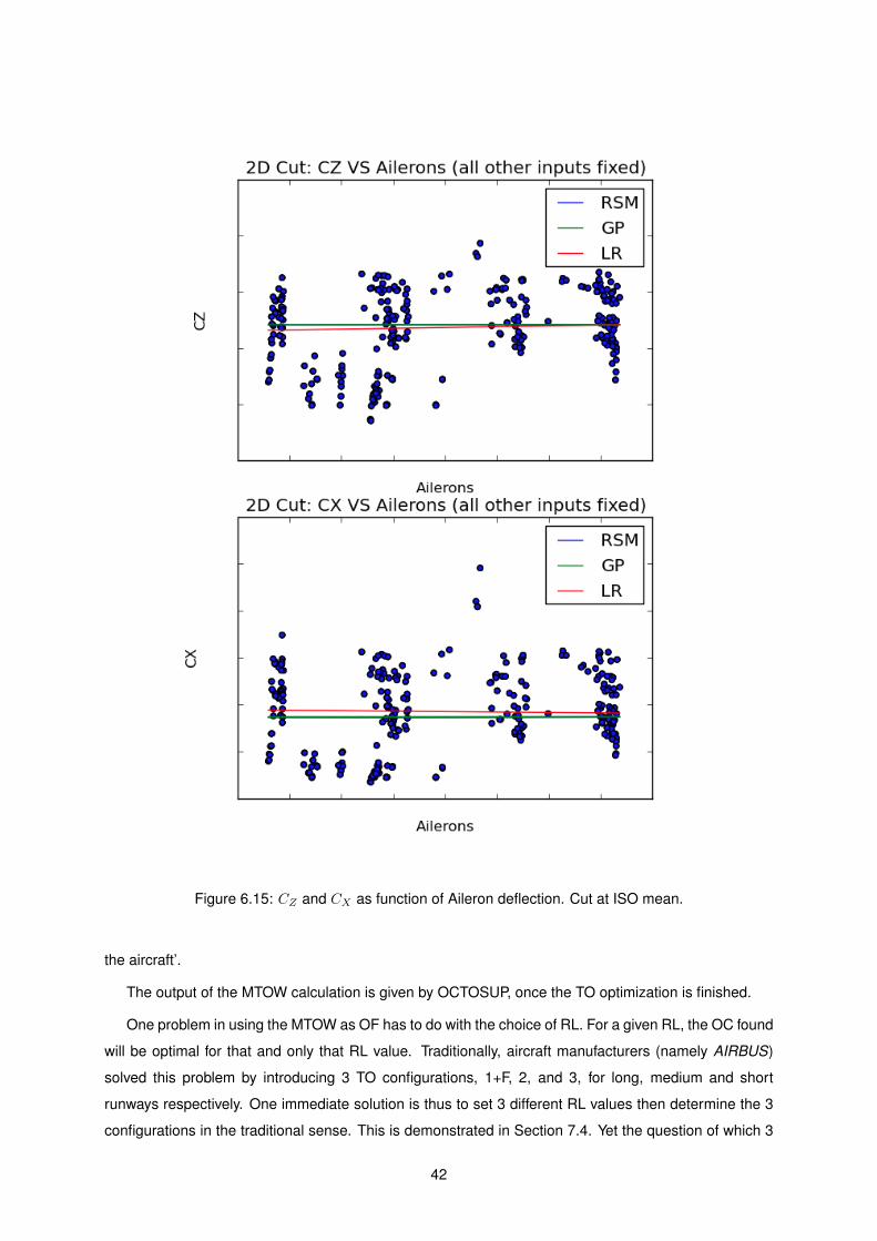
Figure 6.15: CZ and CX as function of Aileron deflection. Cut at ISO mean.
the aircraft’.
The output of the MTOW calculation is given by OCTOSUP, once the TO optimization is finished.
One problem in using the MTOW as OF has to do with the choice of RL. For a given RL, the OC found
will be optimal for that and only that RL value. Traditionally, aircraft manufacturers (namely AIRBUS)
solved this problem by introducing 3 TO configurations, 1+F, 2, and 3, for long, medium and short
runways respectively. One immediate solution is thus to set 3 different RL values then determine the 3
configurations in the traditional sense. This is demonstrated in Section 7.4. Yet the question of which 3
42

Figure 6.16: CZ and CX as function of CG (Center of Gravity) position. Cut at ISO mean.
RL to pick remains. At this stage, engineering experts can come up with educated guesses, wrapping
up the issue for this Objective Function (OF).
However, this OF question begs to be pushed further. Using the OF previously described, the final
aircraft will have 3 TO configurations optimized for 3 different RLs: R1 < R2 < R3. For simplicity, let us
assume R1 = 2000m, R2 = 3000m and R3 = 4000m. Consider now these two scenarios:
• In real life usage, the aircraft will rarely TO from runways measuring exactly R1,R2 or R3 meters.
If, as an example, the aircraft has to serve three airports with 3 RLs R1 = 2500m, R2 = 3500m
43

Figure 6.17: CZ and CX as function of the Engine setting. Cut at ISO mean.
and R3 = 4500m, all its configurations will be non-optimal.
• Suppose the aircraft is to serve 20 airports with RL 4000m and 100 airports with RL 4200m. In
this case, the OC for R1 should really have been defined at a RL closer to 4200m.
These scenarios hint at the need for a more general approach to the OF definition problem. A pos-
sible answer unexpectedly arises from Uncertainty Propagation (UP) methods (see 5), and is detailed
next.
Consider the RL of a given airport served by our aircraft to be a continuous random variable X of
44

Figure 6.18: MTOW calculator architecture.
Figure 6.19: ACZMAX GP SM label CZMAXVS Flap and Slat deflection 3D hyper-cut, at ISO minimum.
unknown distribution, representing the probability of, in case an airport is picked randomly, its RL is near
X. In that case, the MTOW for the hypothetical airport in question will also be a RV, of unknown and
possibly unusual distribution. This distribution is of interest, but before it can be used two questions need
45

(a) CZMAX VS Mach at ISO minimum. (b) CZMAX VS Mach at ISO maximum.
Figure 6.20: Two dimensional visualization of the Mach parameter influence on the ACZMAX label.
to be addressed:
1. How to economically and accurately find the MTOW Distribution (MDist)? It should be reminded
that a TO optimization takes time, and long simulations (using numerous RL values) are unpractical
(read expensive) for a real-time procedure like the CoH.
2. How to exploit this MDist?
Answer to 1 is given by the UP method described in Section 5.2.4. Using only three RL values,
accurate µMDist and σMDist values can be obtained.
Answer to 2 calls for a brief ponderation. The only information about MDist cheaply obtainable are the
µMDist and σMDist moments. Given that nothing else is known about MDist, maximizing or minimizing
σMDist would not be of use. As a measure of dispersion, a bigger σMDist would guarantee an occasional
greater MTOW at the expense of punctual smaller MTOWs. Since aircraft are sold with strict minimum
TOW guarantees for different airports, this maximization could constitute a problem. A minimization
would bring no significant benefits either. Maximizing µMDist, however, is both a simple and relevant
target. It corresponds to finding a OC that would, in average, yield the greatest MTOW at any given
airport. This is the criteria that defined the final choice of OF for the CoH.
Figure 6.21 illustrates the final Objective Calculator architecture that was put into place.
The entries to the module are analogous to those depicted in Fig. 6.18, with the exception of the
Runway range. This is an interval of the form RR = [RLmin, RLmax]. Only airports where RL∈ RR are
considered for uncertainty propagation. It is the input for control of the OF.
In step 1 of UP, the 4 statistical moments µ, σ, γ,Γ (mean, standard deviation, skewness and kurtosis)
of the MDist are computed, taking care to only consider a subset of airport limited by RR. It should be
noted that the Airport Runway Data used to compute these statistical moments comprises a list of only
the airports operated by the aircraft, their RL, as well as the number of flights operated there by time-
period. As a result, the weight or importance attributed to a given runway value X for the distribution is
given by:
Value of X =
ak∑ai=a1
Number of flights operated at ai (6.8)
46

Figure 6.21: Objective Calculator architecture.
Where {a1, a2, ..., ak} is a list of airports with runway length near X. A visualization of the distribution
as well as a histogram are present in Fig.6.22. The distribution was estimated using a Gaussian Kernel
smoothing technique.
Figure 6.22: RL probability density and histogram.
Having this information, the 3 RL values where the TO optimization is to be conducted are calculated
next, using the MTOW calculator described previously.
47

Once all MTOWs are calculated, step 2 of UP deals with the calculation of µMDist and σMDist. For
all practical purposes, µMDist is the output of the Objective Calculator module.
Before closing the module description, a physical interpretation of this statistical objective is due. It
can be said that a statistically optimal configuration for the runway range RR yields the biggest MTOW,
in average, throughout aircraft operation in the airports falling inside the RR range.
6.3.4 Gradient Calculator
In this module, an approximation for the gradient of the OF is calculated at the DoE center P.
First, a LR or RSM-quadratic SM is built using the set of objective values calculated beforehand.
Note that the choice between LR or RSM will depend on the optimal DoE RSM assumption made
before, which itself depends in turn on the chosen value for K1 (Section 6.3.1).
Once the SM surface is constructed, the gradient is trivially determined analytically. For example, for
the LR case (which is the most frequently used case) it follows (Section 3.2.1, LR Model):
Y = Xα+ ε =⇒ ∇Y = α, (6.9)
where α are the coefficients of the LR model.
Now, cases where gradient calculation takes place near the DS border must be carefully considered
and treated. In order to do so, a masking procedure was created, and is described below. Let:
• g1∈ [0, 1] be the near-border parameter. This defines a margin for P to be considered ’near the
border’ of the DS domain. More precisely, P is considered to be bordering the high limit of the k-th
(k ∈ n) dimension of the DS if
|pk − Uk| < g1
(Uk − lk
2
), (6.10)
where Uk, lk, pk are defined as in Section 6.3.1. Similarly, P borders the lower limit of the DS k-th
dimension if
|pk − lk| < g1
(Uk − lk
2
). (6.11)
• P r1,r2,...,roq1,q2,...,qo′denote that P is near the higher limit of DS dimensions r1, r2, ..., ro and near the lower
limit of DS dimensions q1, q2, ..., qo′ , with rs 6= qs ∀s ∈ n (P never near two borders of the domain at
the same time).
• Fk be the gradient flux through the DS k-th dimension at point P. It is defined as Fk = ∇yk|P , with
yk being the k-th component of vector Y .
With these definitions in mind, a masked gradient is defined as ∇Ym = ∇Y · m, where m =
[a1a2 · · · an], ak ∈ {0, 1}. The mask m is calculated as follows:
1. PRQ is calculated, with R = {r1, r2, ...} and Q = {q1, q2, ...} being the sets of dimensions P is
bordering;
2. For each d ∈ (R ∪Q), the d-th component md of the mask is set to zero iff:
48

• d ∈ R and Fd > 0, or
• d ∈ Q and Fd < 0.
If this is not the case, md is set to 1.
This masking of the gradient is necessary for the Line Design process done along the gradient line
as explained in Section 6.3.5.
Finally, the output of this module is then a masked normalized gradient at point P, or ∇Ym(X)
‖∇Ym(X)‖
∣∣∣X=P
.
6.3.5 Line Designer
The Line Designer module aims to produce a set of N points GS = {G1, G2, ..., GN} ∈ DS, with all
the points in GS being along the line of increasing OF values. This line, henceforth referred to as
gradient line (GL), covers the direction defined by the masked gradient of the OF calculated at P, i.e.,∇Ym(X)
‖∇Ym(X)‖
∣∣∣X=P
= ∇G.
The GL can thus be parametrized by a single variable z ∈ R, independently of the DS dimensionality
n:
GL(z) = P + z · ∇G, (6.12)
where z ∈ [ζmin, ζmax], and ζmin, ζmax are a function of P,∇G and the DS boundaries lk, Uk (as defined
in Section 6.3.1).
Calculation of ζmin, ζmax yields the parametrization limits, or the minimum and maximum values ∇G
applied at P can be multiplied by until the DS limits are breached. To carry out this calculation, the
following algorithm was developped:
1. Set ζmax = 0;
2. Set zM = maxk(Uk−lk)‖∇G‖ , X = P + z · ∇G. This ensures X will be a point outside DS, provided
P ∈ DS;
3. Using notation from Section 6.3.4, calculate XRQ . If R and Q are not empty sets, make z = z
2 . Else,
make P = X and ζmax = ζmax + z;
4. If the distance from P to the closest DS border is smaller than the precision required, end ζmax
calculation. Else, return to 1;
5. For ζmin steps 1-3 are analogous, except for X = P +z ·∇ in step 1, which becomes X = P −z ·∇.
This algorithm converges exponentially fast.
Once the ζ are known, sampling of N points along GL is a trivial matter of selecting N values in the
range R = [ζmin, ζmax], as the corresponding points can be calculated via Eq. 6.12. The sampling
method implemented in the CoH is simple: Pick ζmin, ζmax, as well as N-2 randomly-selected points in
R, making the set gs = {ζmin, v1, ..., vN−2, ζmax}.
The output GS of this module is then GS = {G1, G2, ..., GN}, where Gk = GL(gsk) and gsk ∈ gs.
49

6.3.6 Line Builder
The Line Builder is a simple module whose purpose is to produce a SM of the OF (Objective Function)
with its domain restricted to the GL (Gradient Line). This makes the restricted OF (hereby denoted L(x))
a 1-dimensional manifold, with parameterizing variable z ∈ [ζmin, ζmax] as defined in Section 6.3.5.
For construction of the SM, L(x) : R 7−→ R, FT and OF value calculations are carried out at each
point from the Line Designer output set GS. A spline L(x) is built using the SPLT technique described in
Section 3.2.4, with the help of MACROS.
The output of the module is the SPLT SM L(x), represented internally by an array of tension coeffi-
cients.
6.3.7 Line Optimizer
Taking as input the L(x) SM built by the Line Builder, the Line Optimizer’s goal is to find the optimum
objective over L, i.e., X∗ = arg maxX L(X).
L being an analytical SM, optimization is performed near-instantaneously using a Quasi-Newton
descent optimization tool provided by MACROS.
Problems often arise near domain boundaries in optimization problems. For the CoH problem, this
issue arises often. As such, the semi-random sampling method implemented ensures that convergence
is not slowed down when optimizing different L over different iterations of the CoH on a boundary k of
the DS, if the flux Fk is outward-bound. If it is inward-bound, no issue arises since line design will be
done into the domain.
The output of this module is of course X∗.
50

Chapter 7
Results
7.1 Overview
The purpose of this Section is to present and validate the results obtained from the CoH algorithm.
Validation of the results is of paramount importance for an expensive real-time procedure such as the
one developed here. Validation comprises two distinct phases, each accompanied by a set of results:
1. Validation of the core performance calculations, that is, a simple MTOW calculation. Being the
underlying foundation of the CoH, any divergences found here would impact all the subsequent
results.
2. Validation of the process itself, that is, the CoH algorithm. For this, results from CoH executions
are compared to optimum values determined via an ’unlimited-budget’ surrogate modelling. This
consists in using the FT Simulator coupled with the Objective Calculator to exhaustively sample
the DS, a sampling from which a very accurate SM is built. It is over this ’unlimited-budget’ SM
model that optimization is then performed. Optimum obtained this way are considered the true
optimum, against which the CoH output can be meaningfully compared.
Regarding what follows, Section 7.2 addresses the aforementioned phase 1, whilst Sections 7.3-7.5
all tackle phase 2.
7.2 Single MTOW, Fixed Runway
The validation and results analysis process starts with simple MTOW calculations, amounting to testing
of a subpart of the Objective Calculator module. In this Section, 4000m is adopted as RL value, and
other sustained parameters are defined according to the FT data used to build the FT Simulator. As
explained earlier in the present work, no CZMAXFT data was available for the FT Simulator, hence the
4000m RL, assuring the segment under consideration is not limited by CZMAX.
This first MTOW calculation is done at a 1+F Configuration, defined in pre-flight as (Confidential)
Slat deflection, (Confidential) Flap deflection, using the pre-flight model. Next, still at (Confidential),
51

calculations are launched using LR and RSM interpolation techniques for the labels, with a varying
number of interpolation points and full overload of all label models. Results are displayed in Fig. 7.1.
(a) MTOW as function of interpolation technique.
(b) Interpolation error.
Figure 7.1: RSM and LR interpolation results.
See Confidential Appendix, Data 3.
Thus, the question that truly needs to be answered is: which interpolation method better represents
the FT data?
To attempt to answer this, the Lift and Drag polars used by OCTOSUP during the TO optimization
loop for all three cases (pre-flight, LR, RSM) were extracted and visualized (Fig. 7.2). Keep in mind this
was done using 4 different speed measures for each FP.
Bearing in mind that only the continuous, more dense parts of the curves are of importance, two
comments can be made regarding Fig. 7.2:
See Confidential Appendix, Data 4.
A look at the absolute modelling errors involved (Fig. 7.3) yields an important insight into MTOW
calculation sensibility versus label modelling errors.
See Confidential Appendix, Data 5.
This is an aspect of the utmost importance in the CoH algorithm: a proper sampling along the alphas
during FP measurement is vital for result accuracy. A RSM interpolation is adopted in the Sections that
follow.
52

Figure 7.2: Lift and drag (CZ and CX ) curve plots.
Figure 7.3: Lift and drag (CZ and CX ) error analysis.
53

7.3 Optimal Configuration, Fixed Runway
In the present Section, CoH algorithm results are compared against the so-called ’true’ results. These
true results are obtained from optimization over the DS using a SM, which in turn is built for a fixed RL.
This is known as Surrogate-Based Optimization (SBO). The SM takes as input a configuration, and it
outputs the corresponding MTOW. Keep in mind a sampling (training) set of the DS is needed to build
the SM.
At this stage two factors need now to be considered: the sample size S and DoE Technique. Ideally,
for purposes of comparison with CoH results, a SM where S → ∞ with a Full Factorial DoE would be
best, as it would be the closest to reality. However, it is of major interest to determine if a comparable
accuracy could be obtained with a significantly smaller S or not. A small enough S the generates an
accurate SM would qualify this Surrogate-based Optimization process as a worthy alternative to the
CoH.
The S∞ SM, henceforth considered as the reference, was built using a S = 225 FF DoE. From it,
the true OC and respective MTOW for a RL of 4000m were derived, and are both depicted in Figure 7.4.
More precisely, the OC found is indicated in Table 7.1.
Slats –Flaps –MTOW –
Table 7.1: Optimal Configuration for RL 4000m
See Confidential Appendix, Data 6.
A similar process was then carried out using smaller S values and different DoE techniques, taking
care to always sample the entire DS. The results obtained are shown in Figures 7.5 and 7.6.
See Confidential Appendix, Data 7.
54

(a) 3D view.
(b) Top view of the surrogate.
Figure 7.4: MTOW as function of configuration, using GP SM based on FF limit design. Note the OC,indicated by a yellow star.
55

Figure 7.5: MTOW value progression for the full DS, depending on DoE sample size S and technique.
Figure 7.6: Absolute MTOW error for the full DS, depending on DoE sample size S and technique.
56

Figure 7.7: MTOW value progression for a small sampling domain, depending on DoE sample size Sand technique.
Figure 7.8: Absolute MTOW error for a small sampling domain, depending on DoE sample size S andtechnique.
57

Even for a small (Confidential) sample, extremely precise results are obtained, regardless of the DoE
technique used. This fact, coupled with the Slat and Flap configuration convergence depicted in Figs.
7.9 and 7.10 respectively, position small-DS SBO as a valid tool for confirmation purposes. If a very
precise initial guess is already known (from a same-family aircraft, for example) confirmation of the OC
location could be quickly and cheaply carried out this way.
Figure 7.9: Slat deflection for a small sampling domain, depending on DoE sample size S and technique.
58

Figure 7.10: Flap deflection for a small sampling domain, depending on DoE sample size S and tech-nique.
59

At this stage, having obtained the ’true’ OC for reference (Table 7.1), all that is left to determine is the
correct parameterization for the CoH algorithm, namely:
• The minimum number of iterations needed until a satisfactory (small enough) error is obtained;
• Optimal number of Flight Points (FP) to use around each Design Point (DP) for gradient calculation;
• Optimal number of FP to use in the creation of the gradient line.
To accomplish this, a DoE OLHS set was first created using these 3 parameters (NumRuns, DoeSize,
LineSize). Additionally, a set of 10 random start-points (SP) was also created. Then, for each SP and
for each configuration in OLHS set, the CoH algorithm was launched, with the average over the SP set
of the results obtained being used to build a SM.
Figure 7.11 shows the MTOW (objective) evolution versus the number of iterations and DoE size.
Convergence to the true OC MTOW value with the increasing number of runs was expected, and is
clearly observable. Yet, the influence of the DoE size used in gradient calculation is very small, with
bigger gradient DoEs appearing to slightly slow convergence (mayhap due to gradient ’pollution’).
Figure 7.11: 3D GP SM cut at ISO-max of CoH output as function of local DoE pool sample size andnumber of iterations.
60

Similar 3D cuts for the number of points along the gradient line (LineSize) are depicted in Figs. 7.12a
and 7.12b. Besides the convergence with increasing number of iterations, the line size shows this time
a significant influence on convergence speed. The RSM model in Fig. 7.12b underlines this point, better
capturing the trend. Using only (Confidential) points to build the gradient line seems to be something to
avoid.
Concerning convergence speed, that is, how many runs are really needed to attain the true ’OC’, a
2D cut provides a good first answer (see Fig. 7.13). After just (Confidential) iterations, a very precise
estimate is already obtained, improving marginally from there onwards.
61

(a) GP 3D cut.
(b) RSM 3D cut.
Figure 7.12: 3D cuts at ISO-average of CoH output as function of gradient line sample size and numberof iterations.
62

Figure 7.13: 2D cuts showing MTOW convergence with increasing number of iterations.
63

Now, in order to quantify CoH performance, two curves are of paramount importance, and they are
described next:
Error Vs FP Budget
Consider the FP Budget of an entire CoH execution to be defined as
FP Budget = (DoE Size + Nb Grad Line Points)× Nb of Iterations + 1, (7.1)
where the last FP to be evaluated is the last optimum over the gradient line. To obtain a curve
relating the error obtained (compared to the ’true’ OC) with the total number of FP used, the
following optimization problem is posed:
minimized,g,n
FP Budget(d, g, n)
subject to |MTOW (d, g, n)−MTOW ∗| ≤ E, E = e1, . . . , em.
(7.2)
Where d, g are the number of FP used in each DoE and Gradient Line, respectively, and n is the
number of iterations. The problem is solved for different values of admissible error E, namely
e1, . . . , em. The parametric model constructed before is used to carry out the optimization. Recall
that the model was built using results averaged over 10 different random starting points.
Error Vs Number of Runs This second curve is a by-product of the optimization process previously
described, illustrating the effect of the error allowed on the number of CoH iterationS;
Note that curves describing the evolution of d and g also arise naturally from the optimization process.
Everything is depicted in Figures 7.14a and 7.14b.
Figure 7.14a shows results for CoH executions with a large error allowed. Possible conclusions are:
See Confidential Appendix, Data 8.
Analysis of Fig. 7.14b, traced for smaller error allowances, yields greater insights on the aforemen-
tioned results. A number of observations can be made:
See Confidential Appendix, Data 9.
This being said, from a business perspective the fundamental question is the grand total of FP used
to reach the OC. Figure 7.15 attempts to address this question showing the configuration and objective
convergence throughout CoH execution (as the number of FP increases). The green lines are the ’true’
optima.
Once again, after (Confidential) FP a satisfying result is already obtained (less than (Confidential) of
error). Flap behaviour, despite converging, behaves oddly. This can be explained both by the relative
’flatness’ of the objective function near the optimum as well as by the natural oscillations present in the
GP parametric SM used.
64

(a) Large error allowance parameterization results.
(b) Small error allowance parameterization results.
Figure 7.14: CoH full parameterization and run results.
65

(a) CoH Slap deflection convergence.
(b) CoH Flap deflection convergence.
(c) CoH MTOW objective convergence.
Figure 7.15: CoH Configuration and Objective convergence.
66
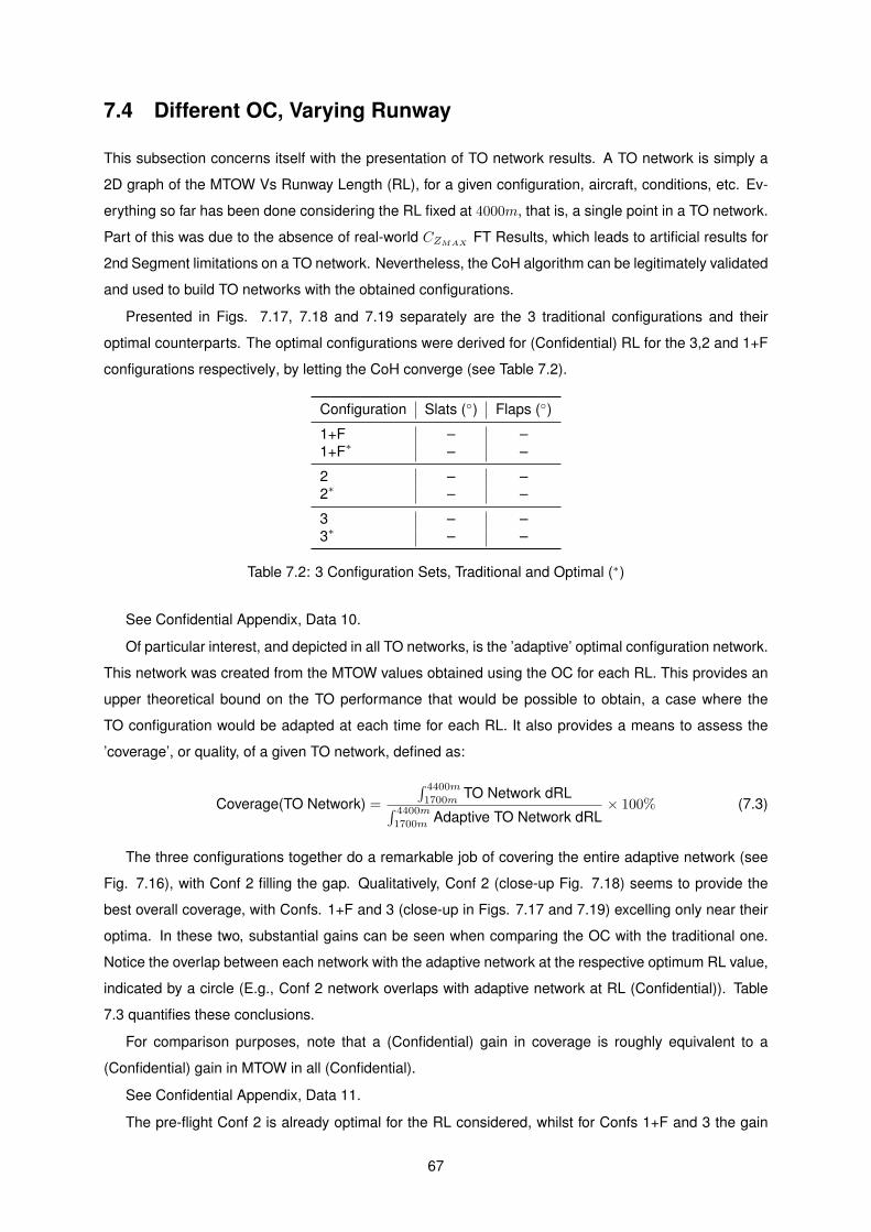
7.4 Different OC, Varying Runway
This subsection concerns itself with the presentation of TO network results. A TO network is simply a
2D graph of the MTOW Vs Runway Length (RL), for a given configuration, aircraft, conditions, etc. Ev-
erything so far has been done considering the RL fixed at 4000m, that is, a single point in a TO network.
Part of this was due to the absence of real-world CZMAXFT Results, which leads to artificial results for
2nd Segment limitations on a TO network. Nevertheless, the CoH algorithm can be legitimately validated
and used to build TO networks with the obtained configurations.
Presented in Figs. 7.17, 7.18 and 7.19 separately are the 3 traditional configurations and their
optimal counterparts. The optimal configurations were derived for (Confidential) RL for the 3,2 and 1+F
configurations respectively, by letting the CoH converge (see Table 7.2).
Configuration Slats (◦) Flaps (◦)
1+F – –1+F∗ – –
2 – –2∗ – –
3 – –3∗ – –
Table 7.2: 3 Configuration Sets, Traditional and Optimal (∗)
See Confidential Appendix, Data 10.
Of particular interest, and depicted in all TO networks, is the ’adaptive’ optimal configuration network.
This network was created from the MTOW values obtained using the OC for each RL. This provides an
upper theoretical bound on the TO performance that would be possible to obtain, a case where the
TO configuration would be adapted at each time for each RL. It also provides a means to assess the
’coverage’, or quality, of a given TO network, defined as:
Coverage(TO Network) =
∫ 4400m
1700mTO Network dRL∫ 4400m
1700mAdaptive TO Network dRL
× 100% (7.3)
The three configurations together do a remarkable job of covering the entire adaptive network (see
Fig. 7.16), with Conf 2 filling the gap. Qualitatively, Conf 2 (close-up Fig. 7.18) seems to provide the
best overall coverage, with Confs. 1+F and 3 (close-up in Figs. 7.17 and 7.19) excelling only near their
optima. In these two, substantial gains can be seen when comparing the OC with the traditional one.
Notice the overlap between each network with the adaptive network at the respective optimum RL value,
indicated by a circle (E.g., Conf 2 network overlaps with adaptive network at RL (Confidential)). Table
7.3 quantifies these conclusions.
For comparison purposes, note that a (Confidential) gain in coverage is roughly equivalent to a
(Confidential) gain in MTOW in all (Confidential).
See Confidential Appendix, Data 11.
The pre-flight Conf 2 is already optimal for the RL considered, whilst for Confs 1+F and 3 the gain
67

Figure 7.16: Traditional and CoH TO complete network coverage for the three different configurations.
Figure 7.17: Traditional and CoH configuration 1+F TO network detail.
68

Figure 7.18: Traditional and CoH configuration 2 TO network detail.
Figure 7.19: Traditional and CoH configuration 3 TO network detail.
69

Configuration Coverage (%) Gain (%)
1+F 97.89881+F∗ 98.6999 +0.8011
2 99.47102∗ 99.4565 -0.01450
3 98.62393∗ 98.9310 +0.3071
1+F and 3 99.57991+F∗ and 3∗ 99.8036 +0.2237
All 99.8157All∗ 99.8971 +0.0814
Table 7.3: Different TO network coverage.
is considerable, as mentioned before. However, considering individual configuration gains may not be
the most appropriate metric to judge a configuration, since those configurations are only expected to
perform well in a vicinity of their respective optimal RLs. Thus, a coverage improvements for Confs
1+F/3 together, as well as for all Confs, are also calculated in Table 7.3. The final gain is small, which
was expected given the use of a pre-flight CZMAX.
Thanks to the adaptive TO network, it is now possible to trace the evolution of the OC deflections
with varying RL. This is shown in Figure 7.20.
Figure 7.20: Optimal Configuration evolution with Runway Length.
See Confidential Appendix, Data 12.
70

7.5 Statistically Optimal Configuration
To go a bit further in the definition of optimal configuration, and as thoroughly discussed in Section 6.3.3,
a redefinition of the objective function was needed. Results using a statistically optimal OF are here pre-
sented and discussed in Table 7.4.
RL Range (m) Slats (◦) Flaps (◦) E(MTOW ) (kg)
[1700, 3000] – – –[3000, 3500] – – –[3500, 4400] – – –[1700, 4400] – – –
Table 7.4: Statistical OC results and their standard counterparts.
See Confidential Appendix, Data 13.
The first column on the left indicates the range of airport RLs that was considered for uncertainty
propagation. The rationale behind the four chosen ranges was simple: picking three ranges that roughly
corresponds to each of the 3 traditional configuration domains and a range encompassing all the domain,
to see which would be the ideal TO configuration if only one configuration was allowed.
The last column on the right is the OF value. In this case, it answers the following question: ”Taking-
Off at random from airports with runway ∈ RL Range, and considering more important airports to have
more TakeOffs, what is the expected average MTOW the aircraft can offer?”
Interestingly enough, the configuration values found for each of the first three ranges are not far from
the corresponding OC found before for the 3 Confs in Table 7.2 in Section 7.4.
See Confidential Appendix, Data 14.
However, the 3 configurations determined before do NOT take into account the runway importance
distribution, making the results obtained even more relevant.
Additionaly, for the full domain range, something close to a Conf 2 avails itself as the optimal con-
figuration. This underscores the previously made remark that the Conf 2 is the configuration with the
highest coverage.
Finally, a word of caution is due. This statistically optimal procedure requires thrice the amount of
time an ordinary CoH execution would, meaning it may render execution in real-time for flight testing
impractical.
71

Chapter 8
Conclusion
The present work’s contribution to the state-of-the-art in the Aircraft Performance domain consisted in
the definition, implementation and validation of a novel gradient-based procedure for systematic deter-
mination of the optimal takeoff configurations of an aircraft. In addition, a second SBO procedure was
proposed, mainly for validation purposes, and its viability was also demonstrated. Both procedures were
shown to not only meet the requirements of finding an optimal solution, but also of making it possible to
do so in an easily extensible and economical way. An innovative statistical objective function was finally
proposed, its merits and feasibility discussed.
Firstly, the main idea behind TO optimization was presented, along with key elements and tech-
niques on surrogate modelling, design of experiment and uncertainty propagation. This comprised the
theoretical backbone of the algorithms implemented.
Next the gradient-based solution architecture, along with its implementation, was described in detail.
The algorithm developed, named CoH for ConfOpt Hunter, was then validated resorting to a second
SBO procedure.
Validation, presentation and discussion of the results and insights discovered was done gradually in
4 steps, synthesized next.
Stage 1 consisted on the validation of simple MTOW calculation capabilities, resorting to surrogate
models to model internal aerodynamic labels. This allowed for MTOW calculation at any given contin-
uous point in the configuration design space. It was found that RSM label interpolation provided better
results than a LR interpolation. The key insight to retain at this stage is the importance of an adequate
representation of the basic aerodynamic coefficients, meaning proper choice of alphas and interpolation
technique, in order to get sensible MTOW values for any general TO configuration. This is true since
relatively small interpolation errors on drag coefficients were found to have a heavy impact on the output.
Stage 2 handled the optimal configuration determination itself, albeit for a fixed runway. At this point,
the viability of a SBO procedure was assessed. This SBO procedure, consisting in sampling the entire
configuration domain and optimizing over a model built from those samples, was also used to evaluate
its gradient-based counterpart. To do this, an extensive sampling pool was used to build a very high-
fidelity model, from which the ’true’ optimum was derived. Using this ’true’ optimum, the gradient method
72

was demonstrated to be a viable and flexible choice to find the OC. However, and this is the key idea to
take from this step, a SBO done over a restricted domain of the design space is also an equally good
alternative for this purpose.
Stage 3 introduced varying runway values, making it possible to validate the CoH algorithm for the
general case. CoH results were used to build different TO networks, and significant gains were shown
to be possible to obtain. The most valuable contribution this step provided was the possibility to trace an
adaptive TO network, that is, a network showing the maximum attainable MTOW at each runway length.
The importance of this adaptive network is significant, as it provides an upper bound against which to
compare all other networks and assess the quality of a particular set of configurations.
The fourth and final step was the statistical objective function definition. Although powerful, due to
the need for more calculations, this statistical OF might prove to be too slow for real-time applications.
Nevertheless, the most important information this step provided was one of confirmation. In other words,
the optima found using this OF are close to those found before, despite the fact that now information
on the relative importance of each runway length is incorporated in the calculation. This valuable infor-
mation was previously ignored. Eventually, this method will allow for slight non-intuitive corrections on
future OC settings.
Despite this being essentially an optimization work, the absolute most valuable insight the project
offered was not one of how much ’better’ the optimal configurations found are. Instead, the current work
proved those optima can be reached faster and cheaper than in the past, using a method that is easily
expandable to any number of problem dimensions. This means that if in the future AIRBUS envisions
optimizing more than 2 parameters for the OC, that can be easily done. Not only that, the methods
implemented, using state-of-art tools, are only the tip of the iceberg regarding the possibilities in this
domain: for example, cruise flight configurations, which resort to Variable Camber (DFS flap settings),
could be optimized using this method.
Future work directions on this topic are thus numerous, with a non-exhaustive list of three examples
reading as follows:
• Determination of an effective real-time alpha/speed selection method for label interpolation, or
interpolation solutions in general. It was found that even minor label interpolation errors could lead
to grave errors in the objective functions. A full-proof method of interpolation would be an essential
first step in rendering the CoH algorithm 100% robust.
• Study of the optimal number of configurations to include in the aircraft. Although the more configu-
rations are included the better the overall coverage of the TO network, these incur extra costs that
are not limited to the Performance domain. The possibility of using only one or two configurations
remains open.
• Algorithm innovations at a real-time level. Due to the real-time nature of flight-testing, different
procedures and/or order of evaluation of FP can be put into place to minimize aircraft idle flight
time.
73

74

Bibliography
[1] S. Koziel, D. E. Ciaurri, and L. Leifsson, “Surrogate-based methods,” in Computational Optimization,
Methods and Algorithms, pp. 33–59, Springer, 2011.
[2] J. Gray, K. T. Moore, T. A. Hearn, and B. A. Naylor, “A standard platform for testing and compari-
son of mdao architectures,” in 8th AIAA multidisciplinary design optimization specialist conference
(MDO), Honolulu, pp. 1–26, 2012.
[3] J. Sacks, W. J. Welch, T. J. Mitchell, and H. P. Wynn, “Design and analysis of computer experi-
ments,” Statistical science, pp. 409–423, 1989.
[4] N. V. Queipo, R. T. Haftka, W. Shyy, T. Goel, R. Vaidyanathan, and P. Kevin Tucker, “Surrogate-
based analysis and optimization,” Progress in aerospace sciences, vol. 41, no. 1, pp. 1–28, 2005.
[5] A. I. Forrester and A. J. Keane, “Recent advances in surrogate-based optimization,” Progress in
Aerospace Sciences, vol. 45, no. 1, pp. 50–79, 2009.
[6] S. R. Schmidt and R. G. Launsby, Understanding industrial designed experiments. Air Academy
Press, 1989.
[7] Z. Qian, C. C. Seepersad, V. R. Joseph, J. K. Allen, and C. J. Wu, “Building surrogate models
based on detailed and approximate simulations,” Journal of Mechanical Design, vol. 128, no. 4,
pp. 668–677, 2006.
[8] A. G. Airbus, Getting to Grips with Aircraft Performance. Customer Services, Blagnac, 2002.
[9] J. A. Authorities, “Joint aviation requirements. jar-25. large aeroplanes,” Civil Aviation Authority
Printing & Publication Services, Greville House, vol. 37, 1994.
[10] A. Forrester, A. Sobester, and A. Keane, Engineering design via surrogate modelling: a practical
guide. John Wiley & Sons, 2008.
[11] T. Hastie, R. Tibshirani, J. Friedman, and J. Franklin, “The elements of statistical learning: data
mining, inference and prediction,” The Mathematical Intelligencer, vol. 27, no. 2, pp. 83–85, 2005.
[12] G. E. Box and N. R. Draper, Empirical model-building and response surfaces. John Wiley & Sons,
1987.
[13] C. L. Lawson and R. J. Hanson, Solving least squares problems, vol. 161. SIAM, 1974.
75

[14] E. Burnaev, M. Belyaev, and A. Lyubin, “Construction of approximation based on linear expansion
in heterogeneous nonlinear functions,”
[15] T. Zou, M. Cai, and X. Shu, “Response surface methodology and improved interval analysis
method—for analyzing uncertainty in accident reconstruction,” Forensic science international,
vol. 222, no. 1, pp. 306–312, 2012.
[16] R. H. Myers, D. C. Montgomery, and C. M. Anderson-Cook, Response surface methodology: pro-
cess and product optimization using designed experiments, vol. 705. John Wiley & Sons, 2009.
[17] M. L. Stein, Interpolation of spatial data: some theory for kriging. Springer, 1999.
[18] N. Cressie, “The origins of kriging,” Mathematical geology, vol. 22, no. 3, pp. 239–252, 1990.
[19] C. Paciorek and M. Schervish, “Nonstationary covariance functions for gaussian process regres-
sion,” Advances in neural information processing systems, vol. 16, pp. 273–280, 2004.
[20] P. C. Mahalanobis, “On the generalized distance in statistics,” Proceedings of the National Institute
of Sciences (Calcutta), vol. 2, pp. 49–55, 1936.
[21] C. K. Williams and C. E. Rasmussen, “Gaussian processes for machine learning,” the MIT Press,
vol. 2, no. 3, p. 4, 2006.
[22] R. Renka, “Interpolatory tension splines with automatic selection of tension factors,” SIAM Journal
on Scientific and Statistical Computing, vol. 8, no. 3, pp. 393–415, 1987.
[23] S. Pruess, “An algorithm for computing smoothing splines in tension,” Computing, vol. 19, no. 4,
pp. 365–373, 1978.
[24] L. Finschi, “Quasi-monte carlo: An empirical study on low-discrepancy sequences,” tech. rep.,
Working paper, Swiss Federal Institute of Technology, 1996.
[25] F. A. C. Viana, V. Steffen Jr, G. Venter, and V. Balabanov, “On how to implement an affordable
optimal latin hypercube,” 2007.
[26] H. Faure, “Discrepance de suites associees a un systeme de numeration (en dimension s),” Acta
Arithmetica, vol. 41, no. 4, pp. 337–351, 1982.
[27] J. H. Halton, “Algorithm 247: Radical-inverse quasi-random point sequence,” Communications of
the ACM, vol. 7, no. 12, pp. 701–702, 1964.
[28] I. M. Sobol, “Uniformly distributed sequences with an additional uniform property,” USSR Compu-
tational Mathematics and Mathematical Physics, vol. 16, no. 5, pp. 236–242, 1976.
[29] M. Stein, “Large sample properties of simulations using latin hypercube sampling,” Technometrics,
vol. 29, no. 2, pp. 143–151, 1987.
[30] J. C. Helton and F. J. Davis, “Latin hypercube sampling and the propagation of uncertainty in analy-
ses of complex systems,” Reliability Engineering & System Safety, vol. 81, no. 1, pp. 23–69, 2003.
76

[31] R. L. Iman, Latin hypercube sampling. Wiley Online Library, 2008.
[32] J.-S. Park, “Optimal latin-hypercube designs for computer experiments,” Journal of statistical plan-
ning and inference, vol. 39, no. 1, pp. 95–111, 1994.
[33] F. A. Viana, “Things you wanted to know about the latin hypercube design and were afraid to ask,”
in 10th World Congress on Structural and Multidisciplinary Optimization, Orlando, Florida, USA (cf.
p. 69), 2013.
[34] Proceedings of the 58th ISI world statistics congress, (Dublin, Ireland), 2011.
[35] R. S. John and N. R. Draper, “D-optimality for regression designs: a review,” Technometrics, vol. 17,
no. 1, pp. 15–23, 1975.
[36] H. Dette and T. E. O’Brien, “Optimality criteria for regression models based on predicted variance,”
Biometrika, vol. 86, no. 1, pp. 93–106, 1999.
[37] N.-K. Nguyen and A. J. Miller, “A review of some exchange algorithms for constructing discrete
d-optimal designs,” Computational Statistics & Data Analysis, vol. 14, no. 4, pp. 489–498, 1992.
[38] W. Chen, J. K. Allen, K.-L. Tsui, and F. Mistree, “A procedure for robust design: minimizing varia-
tions caused by noise factors and control factors,” Journal of Mechanical Design, vol. 118, no. 4,
pp. 478–485, 1996.
[39] G.-J. Park, T.-H. Lee, K. H. Lee, and K.-H. Hwang, “Robust design: an overview,” AIAA journal,
vol. 44, no. 1, pp. 181–191, 2006.
[40] M. Padulo, M. S. Campobasso, and M. D. Guenov, “Novel uncertainty propagation method for robust
aerodynamic design,” AIAA journal, vol. 49, no. 3, pp. 530–543, 2011.
[41] P. Mattia, C. M. Sergio, G. M. Dimitrov, et al., “Comparative analysis of uncertainty propagation
methods for robust engineering design,” Guidelines for a Decision Support Method Adapted to
NPD Processes, 2007.
[42] L. Lewis and A. Parkinson, “Robust optimal design using a second-order tolerance model,” Re-
search in Engineering Design, vol. 6, no. 1, pp. 25–37, 1994.
[43] L. L. Green, H.-Z. Lin, and M. R. Khalessi, “Probabilistic methods for uncertainty propagation ap-
plied to aircraft design,” AIAA Paper, vol. 3140, p. 2002, 2002.
[44] A. Parkinson, C. Sorensen, and N. Pourhassan, “A general approach for robust optimal design,”
Journal of Mechanical Design, vol. 115, no. 1, pp. 74–80, 1993.
[45] S. J. Julier and J. K. Uhlmann, “A general method for approximating nonlinear transformations
of probability distributions,” tech. rep., Technical report, Robotics Research Group, Department of
Engineering Science, University of Oxford, 1996.
77

[46] H. Xu and S. Rahman, “A generalized dimension-reduction method for multidimensional integra-
tion in stochastic mechanics,” International Journal for Numerical Methods in Engineering, vol. 61,
no. 12, pp. 1992–2019, 2004.
[47] M. Cioffi, A. Formisano, R. Martone, G. Steiner, and D. Watzenig, “A fast method for statistical
robust optimization,” Magnetics, IEEE Transactions on, vol. 42, no. 4, pp. 1099–1102, 2006.
[48] D. G. Luenberger, Introduction to linear and nonlinear programming, vol. 28. Addison-Wesley Read-
ing, MA, 1973.
[49] J. Snyman, Practical mathematical optimization: an introduction to basic optimization theory and
classical and new gradient-based algorithms, vol. 97. Springer, 2005.
[50] P. Wolfe, “Convergence conditions for ascent methods,” SIAM review, vol. 11, no. 2, pp. 226–235,
1969.
78