Journal of Water Resource and Protection, 2015, 7, 715-729 Published Online July 2015 in SciRes. http://www.scirp.org/journal/jwarp http://dx.doi.org/10.4236/jwarp.2015.79059

How to cite this paper: Mansouri, R., Torabi, H., Hoseini, M. and Morshedzadeh, H. (2015) Optimization of the Water Dis-tribution Networks with Differential Evolution (DE) and Mixed Integer Linear Programming (MILP). Journal of Water Re-source and Protection, 7, 715-729. http://dx.doi.org/10.4236/jwarp.2015.79059

Optimization of the Water Distribution Networks with Differential Evolution (DE) and Mixed Integer Linear Programming (MILP)

Ramin Mansouri1, Hasan Torabi1, Mohammd Hoseini1, Hosein Morshedzadeh2 1Water Engineering Department, Lorestan University, Khoram Abad, Iran 2Economics and Management Department, Tehran University, Tehran, Iran Email: ramin_mansouri@yahoo.com Received 20 April 2015; accepted 6 July 2015; published 9 July 2015

Copyright © 2015 by authors and Scientific Research Publishing Inc. This work is licensed under the Creative Commons Attribution International License (CC BY). http://creativecommons.org/licenses/by/4.0/

Abstract

Nowadays, due to increasing population and water shortage and competition for its consumption, especially in the agriculture, which is the largest consumer of water, proper and suitable utilization and optimal use of water resources is essential. One of the important parameters in agriculture field is water distribution network. In this research, differential evolution algorithm (DE) was used to optimize Ismail Abad water supply network. This network is pressurized network and includes 19 pipes and 18 nodes. Optimization of the network has been evaluated by developing an optimization model based on DE algorithm in MATLAB and the dynamic connection with EPANET software for network hydraulic calculation. The developing model was run for the scale factor (F), the crossover constant (Cr), initial population (N) and the number of generations (G) and was identified best adeptness for DE algorithm is 0.6, 0.5, 100 and 200 for F and Cr, N and G, respec-tively. The optimal solution was compared with the classical empirical method and results showed that Implementation cost of the network by DE algorithm 10.66% lower than the classical empiri-cal method.

Keywords

Differential Evolution Algorithm, Optimization, Distribution Systems, Crossover Constant, Scale Factor

R. Mansouri et al.

716

1. Introduction Nowadays, due to increasing population and water shortage and competition for its consumption, proper and suitable utilization and optimal use of water resources is essential. Distribution networks are an essential part of all water supply systems. A water distribution network is a system containing pipes, reservoirs, pumps, and valves of different types, which are connected to each other to provide water to consumers.

The water distribution system is one of the major requirements in urban and regional economic development. For any agency dealing with the design of the water distribution network, an economic design will be an objec-tive. Attempts should be made to reduce the cost and energy consumption of the distribution system through op-timization in analysis and design. A water distribution network that includes booster pumps mounted in the pipes, pressure reducing valves, and check-valves can be analyzed by several common methods such as Hardy- Cross, linear theory, and Newton-Raphson (Stephenson, [1]).

Traditionally, pipe diameters are chosen according to the average economical velocities (Hardy-Cross method) (Cross, [2]). This procedure is cumbersome, uneconomical, and requires trials, seldom leading to an economical and technical optimum.

In the case of the design of a pipe network the optimization problem can be stated as follows: minimize the cost of the network components subject to the satisfactory performance of the water distribution system (mainly, the satisfaction of the allowable pressures).

Numerous optimization techniques are used in water distribution systems. These include the deterministic op-timization techniques such as linear programming (for separable objective functions and linear constraints), and non-linear programming (when the objective function and the constraints are not all in the linear form), and the stochastic optimization techniques such as genetic algorithms, simulated annealing, Deferential Algorithm, Par-ticle Swarm Optimization and etc.

Numerous works were reported in the literature for optimal design and some of them considered certain relia-bility aspects too. In optimization models, continuous diameters (Pitchai [3]; Jacoby [4]; Varma et al. [5]) and split pipes (Alperovits & Shamir [6]; Quindry et al. [7]; Goulter et al. [8]; Fujiwara et al. [9] [10]; Kessler & Shamir [11]; Bhave & Sonak [12]) were more prominently used.

Mays and Tung [13] recommended strongly the use of the linear programming (LP) technique in designing the pipe networks due to the capability of the LP in handling more decision variables than other optimization techniques. Dandy and Hassanli [14] developed a nonlinear model for optimum design and operation of multiple subunit drip irrigation systems on flat terrains.

Applications of the genetic algorithm (Dandy and Hassanli [14]; Savic & Walters [15]; Vairavamoorthy & Ali [16] [17]), the modified genetic algorithm (Montesinos et al. [18]; Neelakantan & Suribabu [19]; Kadu et al. [20]), the simulated annealing algorithm (Cunha & Sousa [21]), the shuffled leapfrog algorithm (Eusuff & Lan-sey [22]), ant colony optimization (Maier et al. [23]; Zecchin et al. [24]; Ostfeld & Tubaltzev [25]), novel cellu-lar automata (Keedwell & Khu [26]) and the particle swarm algorithm (Suribabu & Neelakantan [27] [28]) for optimal design of water distribution systems are some of them.

Mansouri et al. [29] by using differential evolution algorithm (DE), CU equation (water distribution unifor-mity coefficient in zb sprinkler irrigation) was optimized and the best optimized coefficients obtained.

Shahinezhad et al. [30] presented a mixed integer linear programming (MILP) model for optimization of pressurized branched irrigation networks. Detailed analysis of the results is reported and compared with those generated based on trial-and-error method. The proposed method results in a reduction of 12.5% in costs.

In this paper, DE algorithm is developed to obtain the optimum pipe size and inlet pressure head that produce the least cost design of Shahinezhad et al. [30] networks. In this study, the hydraulic analysis of the network is based on continuity at nodes and Hazen-Williams formula for head loss calculations by using link between Epanet and Matlab Software. The results of this investigation compared with absolute optimization are obtained by mixed integer linear programming (MILP) model that is presented by Shahinezhad et al. [30].

2. Material and Methods 2.1. Case Study The Ismail Abad irrigation network is located in 7 kilometers North West of Noorabad city in Lorestan province. Land area of this project is 1000 ha. Figure 1 depicts the schematic network of Ismael Abad. This network

R. Mansouri et al.

717

Figure 1. Ismael Abad water distribution network.

consists of 18 pipes and 19 nodes are. In Table 1, the hydraulic details and arrangement of pipes for water dis-tribution networks Ismael Abad is presented.

This project consists of two kinds of steel pipe that is used. Polyethylene pipe material is used for pipe sizes equal or less than 500 mm and GRP for greater sizes. Pipe specifications are given in Table 2.

2.2. Water Distribution Network Constraints 2.2.1. Pressure Constraint Minimum Allowable pressure head required for each node is considered to be 50 m.

2.2.2. Velocity Constraint In order to prevent sediment deposition in low flow velocities and avoid water hammer at high velocities, mini-mum and maximum allowable flow velocities in pipes are considered to be 0.7 m/s and 2 m/s, respectively.

2.3. Differential Evolution Algorithm (DE) Differential Evolution (DE) algorithm is a branch of evolutionary programming developed by Rainer Storn and Kenneth Price [31] [32] for optimization problems over continuous domains. In DE, each variable’s value is represented by a real number. The advantages of DE are its simple structure, ease of use, speed and robustness. DE is one of the best genetic type algorithms for solving problems with the real valued variables. Differential Evolution is a design tool of great utility that is immediately accessible for practical applications. DE has been used in several science and engineering applications to discover effective solutions to nearly intractable prob-lems without appealing to expert knowledge or complex design algorithms. Differential Evolution uses mutation as a search mechanism and selection to direct the search toward the prospective regions in the feasible region. Genetic Algorithms generate a sequence of populations by using selection mechanisms. Genetic Algorithms use

R. Mansouri et al.

718

Table 1. Main and sub main pipe line data of Ismail Abad Network.

Pipe Pipe No. Length (m) Discharge (L/s) Beginning Elevation (m) End Elevation (m)

Res.-J1 P1 - - - -

J2-J3 P2 558 856.56 1791 1816.54

J3-J4 P3 558 856.56 1816.54 1842.08

J4-J5 P4 1430 429.8 1842.08 1847.57

J4-J6 P5 955 52.9 1842.08 1838.71

J4-J7 P6 1100 128.94 1842.08 1856.52

J4-J8 P7 200 244.92 1842.08 1847.05

J8-J9 P8 201 190.34 1847.05 1846.32

J9-J10 P9 390 128.94 1846.32 1841.18

J10-J11 P10 806 58.33 1841.18 1811.32

J11-J12 P11 575 21.49 1811.32 1810.94

J5-J13 P12 550 165.8 1847.57 1853.21

J13-J14 P13 700 132 1853.21 1861.89

J5-J15 P14 670 98.24 1847.57 1821.48

J15-J16 P15 840 33.77 1821.48 1814.43

J5-J17 P16 720 119.73 1847.57 1826.47

J17-J18 P17 660 49.12 1826.47 1847.95

J5-J19 P18 110 46.05 1847.57 1847.57

Table 2. Pipe specifications data of Ismail Abad Network.

Cost ($/m) Outer Diameter (mm) Internal Diameter (mm) Material No.

5.895 110 93.8 PE80 1

7.895 125 106.6 PE80 2

9.495 140 119.4 PE80 3

12.375 160 136.4 PE80 4

15.705 180 153.4 PE80 5

19.305 200 170.6 PE80 6

24.525 225 191.8 PE80 7

30.150 250 213.2 PE80 8

37.800 280 238.8 PE80 9

47.700 319 268.6 PE80 10

60.525 355 302.8 PE80 11

76.725 400 341.2 PE80 12

97.200 450 383.8 PE80 13

108.820 500 426.4 PE80 14

111.323 600 600.0 GRP 15

137.997 700 700.0 GRP 16

170.633 800 800.0 GRP 17

204.289 900 900.0 GRP 18

R. Mansouri et al.

719

crossover and mutation as search mechanisms. The principal difference between Genetic Algorithms and Diffe-rential Evolution is that Genetic Algorithms rely on crossover, a mechanism of probabilistic and useful ex-change of information among solutions to locate better solutions, while evolutionary strategies use mutation as the primary search mechanism.

Differential Evolution (DE) is a parallel direct search method which utilizes NP D-dimensional parameter vectors.

, , 1, 2, ,i Gx i NP= (1)

As a population for each generation G. NP does not change during the minimization process. The initial vec-tor population is chosen randomly and should cover the entire parameter space. As a rule, we will assume a uni-form probability distribution for all random decisions unless otherwise stated. In case a preliminary solution is available, the initial population might be generated by adding normally distributed random deviations to the no-minal solution xnom,0. DE generates new parameter vectors by adding the weighted difference between two pop-ulation vectors to a third vector. Let this operation be called mutation. The mutated vector’s parameters are then mixed with the parameters of another predetermined vector, the target vector, to yield the so-called trial vector. Parameter mixing is often referred to as “crossover” in the ES-community and will be explained later in more detail. If the trial vector yields a lower cost function value than the target vector, the trial vector replaces the target vector in the following generation. This last operation is called selection. Each population vector has to serve once as the target vector so that NP competitions take place in one generation. More specifically DE’s ba-sic strategy can be described as follows:

2.3.1. Mutation For each target vector , , 1, 2, ,i Gx i NP= , a mutant vector is generated according to:

( ), 1 1, 2, 3,i G r G r G r GV x F x x+ = + × − (2)

With random indexes r1, r2, r3 ∈ {1, 2, ⋅⋅⋅, NP} integer, mutually different and F > 0. The randomly chosen integers r1, r2 and r3 are also chosen to be different from the running index i, so that NP must be greater or equal to four to allow for this condition. F is a real and constant factor ∈ [0, 2] which controls the amplification of the differential variation (xr2,G − xr3,G). Figure 2 shows a two-dimensional example that illustrates the differ-ent vectors which play a part in the generation of Vi,G+1.

2.3.2. Crossover In order to increase the diversity of the perturbed parameter vectors, crossover is introduced. To this end, the tri-al vector:

( ), 1 1 , 1 2 , 1 , 1, , ,i G i G i G Di Gu u u u+ + + += (3)

Is formed, where:

( ) ( ), 1, 1

,

if randb or ranbr 1, 2, , .

otherwise ji G

ji Gji G

V j CR j iu j D

x+

+

≤ == =

(4)

In Equation (5), randb(j) is the jth evaluation of a uniform random number generator with outcome ∈ [0; 1]. CR is the crossover constant ∈[0; 1] which has to be determined by the user. rnbr(i) is a randomly chosen index ∈ 1, 2, …, D which ensures that ui,G+1 gets at least one parameter from Vi,G+1.

2.3.3. Selection To decide whether or not it should become a member of generation G + 1, the trial vector ui,G+1 is compared to the target vector xi,G using the greedy criterion. If vector ui,G+1 yields a smaller cost function value than xi,G, then xi,G+1 is set to ui,G+1; otherwise, the old value xi,G is retained.

( ) ( ), 1 , 1 ,, 1

,

if

if otherwise ji G i G i G

ji Gji G

u f u f xx

x+ +

+

≤=

(5)

R. Mansouri et al.

720

Figure 2. An example of a two-dimensional cost function showing its contour lines and the process for generating Vi,G+1.

Finally, this process continues to reach new generations to the number of NP. Then the same process is re-

peated to reach termination condition. Figure 3 schematically overview of differential evolution algorithm for numerical model, the entire above

process is specified numerically in this figure.

2.4. Mixed Integer Linear Programming (MILP) In general, an optimization problem either linear or nonlinear consists of an objective function which is sub-jected to some constraints. The classical linear optimization method may results in a branch which consists of many pipe sizes. In practice, this is considered as a strong weak point. On the other hand, linear optimization methods yields pipe sizes which are not commercially available. This leads to choose the pipe size close to that obtained by optimization. Consequently, the hydraulic conditions and cost of the network system will be differ-ent from that obtained by the optimization technique which means that the design is not optimum any more. The developed model guarantees obtaining the global optimum of pressurized branched irrigation networks.

Objective Function The total annual cost of a pressurized branched irrigation network system can be introduced as:

( ) ( ) ( )1 1

NP NPU

i i i I en PIi I

f D L CP CRF CPU CRF C H= =

= ⋅ ⋅ + ⋅ + ⋅∑ ∑ (6)

where, LN = length of pipe number N, N = subscript representing pipe number in the network, CPN = unit length cost of pipe N, which is a function of pipe diameter, NP = Number of pipes, CPUI = cost of the Ith pump which is a function of the total power of the pump required, NPU = Number of pumps in the network system, Cen = annual energy cost per unit head,

The annual energy cost per unit head of the pump can be expressed as:

e102fu s t

en

C Q Q EAEC

η⋅ ⋅ ⋅

= (7)

In which, Cfu is the fuel cost ($/kWh); Ot is the number of annual system operating in hours; EAE is the equivalent annualized escalating energy cost factor; ηe is the overall pump efficiency in fraction.

( ) ( )( ) ( ) ( )1 e 11 e 1 1 1

y y

y

r rEAEr r

+ − +=

+ − + + − (8)

R. Mansouri et al.

721

Figure 3. Computational module for differential evolution algorithm.

R. Mansouri et al.

722

In which, e is the decimal equivalent annual rate of energy escalation; y is the life time of the design in years, and r is the decimal equivalent annual interest rate. HPI = total dynamic head of the Ith pump, CRF = capital re-turn factor which is calculated as below:

( )( )

1

1 1

y

y

r rCRF

r

+=

+ − (9)

I ICPU P K= ⋅ (10) where, PI = total power of the Ith pump and K = pump station cost per unit total power ($/KW).

Multiplying the terms of the first summation of equation (1) by zero-unity variables such as XNJ, and adding for all commercially available pipes yields:

( ) ( ) ( ), ,1 1 1

NP ND NPU

i i i j i j I en PIi j I

f D L CP CRF X CPU CRF C H= = =

= ⋅ ⋅ ⋅ + ⋅ + ⋅∑∑ ∑ (11)

ND = number of commercially available pipe Diameter, Shahinezhad et al. [30] to ensure of performance the model, MILP model was used for four different branch

network. This study showed that MILP method, with the above objective function is the ability to provide abso-lute optimum for branch network.

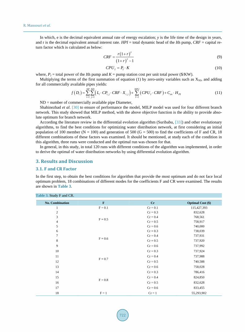
According the literature review in the differential evolution algorithm (Suribabu, [33]) and other evolutionary algorithms, to find the best conditions for optimizing water distribution network, at first considering an initial population of 100 member (N = 100) and generation of 500 (G = 500) to find the coefficients of F and CR, 18 different combinations of these factors was examined. It should be mentioned, at study each of the condition in this algorithm, three runs were conducted and the optimal run was chosen for that.

In general, in this study, in total 120 runs with different conditions of the algorithm was implemented, in order to derive the optimal of water distribution networks by using differential evolution algorithm.

3. Results and Discussion 3.1. F and CR Factor In the first step, to obtain the best conditions for algorithm that provide the most optimum and do not face local optimum problem, 18 combinations of different modes for the coefficients F and CR were examined. The results are shown in Table 3.

Table 3. Study F and CR.

No. Combination F Cr Optimal Cost ($) 1 F = 0.1 Cr = 0.1 115,427,393 2

F = 0.5

Cr = 0.3 832,628 3 Cr = 0.4 768,561 4 Cr = 0.5 758,917 5 Cr = 0.6 740,000 6

F = 0.6

Cr = 0.3 738,039 7 Cr = 0.4 737,931 8 Cr = 0.5 737,920 9 Cr = 0.6 737,992 10

F = 0.7

Cr = 0.3 737,924 11 Cr = 0.4 737,988 12 Cr = 0.5 740,588 13 Cr = 0.6 758,028 14

F = 0.8

Cr = 0.3 786,416 15 Cr = 0.4 824,850 16 Cr = 0.5 832,628 17 Cr = 0.6 833,455 18 F = 1 Cr = 1 55,293,902

R. Mansouri et al.

723

The Results show that median values for the coefficients of F and Cr provide the optimum situation and cause DE algorithm not to be trapped in local optimum. The most optimal answers for coefficients are 0.6 and 0.5 for F and Cr coefficients, respectively. These values matched with the results of Suribabu [33].

Scale factor (F) can increase the accuracy of the search. The smaller coefficient, the shorter steps needs to be taken for an accurate research. But the problem is that the algorithm may be trapped in local optimum and it cannot be withdrawn. On the other hand, the higher value of F, the more area will be searched, but the best op-timum situation may not be obtained.

3.2. Population and Generation After finding the best combination of coefficients values F and CR, algorithms for solving the independent pop-ulations were examined. For this purpose, the population of 4, 25, 50, 100, 500 and 1000 members were studied in two generations (G = 50 and 100). Figure 3 shows these results.

Based on the DE algorithm, the initial population is very important to select the initial three members, when the population gets more, the selection of four initial members has more variety, which causes the algorithm to reach convergence.

According to Figure 4, it is clear that by increasing population, the optimal cost will be lower. In addition It is proved that the increasing population will extend the domain of the search; and more members are used for op-timization.

Finally, the best combination of coefficients and population were used to examine the effect of generations’ number, so ten generations (30, 40, 50, 100, 200, 300, 500, 1000, 2000, and 3000) were studied. The results are shown in Table 4.

Figure 4. Optimization cost in different populations.

Table 4. The effect of generation on optimization cost.

No. Generation Optimal cost ($) Runtime (s)

30 55,293,902 629

40 2,065,347 780

50 1,222,823 1005

100 786,416 1950

200 737,920 4024

300 737,931 6164 500 737,920 9324

1000 737,924 20,163

2000 737,920 39,826

3000 737,920 53,911

R. Mansouri et al.

724

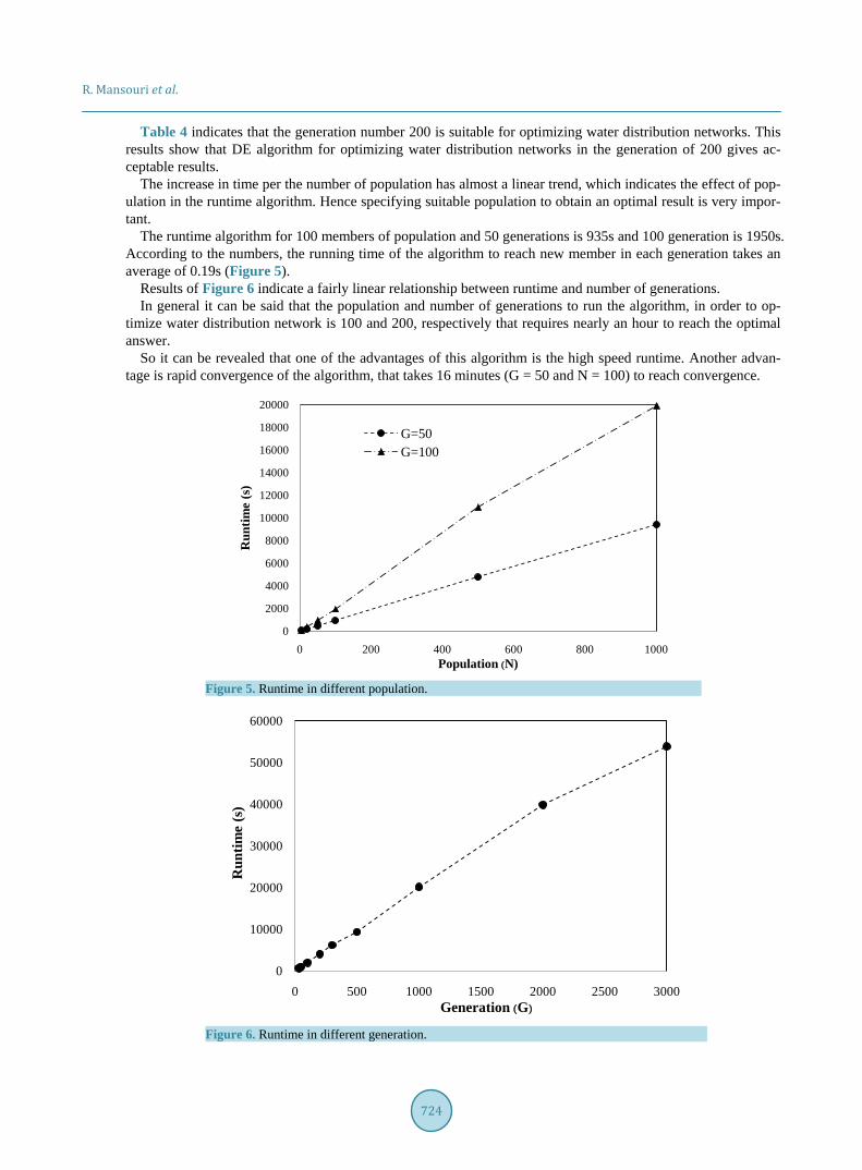
Table 4 indicates that the generation number 200 is suitable for optimizing water distribution networks. This results show that DE algorithm for optimizing water distribution networks in the generation of 200 gives ac-ceptable results.

The increase in time per the number of population has almost a linear trend, which indicates the effect of pop-ulation in the runtime algorithm. Hence specifying suitable population to obtain an optimal result is very impor-tant.

The runtime algorithm for 100 members of population and 50 generations is 935s and 100 generation is 1950s. According to the numbers, the running time of the algorithm to reach new member in each generation takes an average of 0.19s (Figure 5).

Results of Figure 6 indicate a fairly linear relationship between runtime and number of generations. In general it can be said that the population and number of generations to run the algorithm, in order to op-

timize water distribution network is 100 and 200, respectively that requires nearly an hour to reach the optimal answer.

So it can be revealed that one of the advantages of this algorithm is the high speed runtime. Another advan-tage is rapid convergence of the algorithm, that takes 16 minutes (G = 50 and N = 100) to reach convergence.

Figure 5. Runtime in different population.

Figure 6. Runtime in different generation.

0

2000

4000

6000

8000

10000

12000

14000

16000

18000

20000

0 200 400 600 800 1000

Run

time

(s)

)N(Population

G=50G=100

0

10000

20000

30000

40000

50000

60000

0 500 1000 1500 2000 2500 3000

Run

time

(s)

)G(Generation

R. Mansouri et al.

725

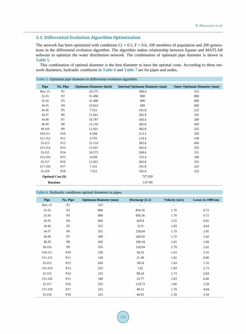
3.3. Differential Evolution Algorithm Optimization The network has been optimized with conditions Cr = 0.5, F = 0.6, 100 members of population and 200 genera-tions in the differential evolution algorithm. The algorithm makes relationship between Epanet and MATLAB software to optimize the water distribution network. The combination of optimum pipe diameter is shown in Table 5.

This combination of optimal diameter is the best diameter to have the optimal costs. According to these net-work diameters, hydraulic conditions in Table 6 and Table 7 are for pipes and nodes.

Table 5. Optimum pipe diameter in differential evolution algorithm.

Pipe No. Pipe Optimum Diameter (inch) Internal Optimum Diameter (mm) Outer Optimum Diameter (mm) Res.-J1 P1 10.575 268.6 315 J2-J3 P2 31.496 800 800 J3-J4 P3 31.496 800 800 J4-J5 P4 23.622 600 600 J4-J6 P5 7.551 191.8 225 J4-J7 P6 11.921 302.8 355 J4-J8 P7 16.787 426.4 500 J8-J9 P8 15.110 383.8 450

J9-J10 P9 11.921 302.8 355 J10-J11 P10 8.394 213.2 250 J11-J12 P11 4.701 119.4 140 J5-J13 P12 15.110 383.8 450 J13-J14 P13 11.921 302.8 355 J5-J15 P14 10.575 268.6 315 J15-J16 P15 6.039 153.4 180 J5-J17 P16 11.921 302.8 355 J17-J18 P17 7.551 191.8 225 J5-J19 P18 7.551 191.8 225 Optimal Cost ($) 737,920

Runtime 1:07:00

Table 6. Hydraulic conditions optimal diameters in pipes.

Pipe No. Pipe Optimum Diameter (mm) Discharge (L/s) Velocity (m/s) Losses in 1000 (m) Res.-J1 P1 315 - - - J2-J3 P2 800 856.56 1.70 0.72 J3-J4 P3 800 856.56 1.70 0.72 J4-J5 P4 600 429.8 1.52 0.81 J4-J6 P5 225 52.9 1.83 4.64 J4-J7 P6 355 128.94 1.79 2.45 J4-J8 P7 500 244.92 1.72 1.62 J8-J9 P8 450 190.34 1.65 1.69

J9-J10 P9 355 128.94 1.79 2.61 J10-J11 P10 250 58.33 1.63 3.32 J11-J12 P11 140 21.49 1.92 8.80 J5-J13 P12 450 165.8 1.43 1.31 J13-J14 P13 355 132 1.83 2.73 J5-J15 P14 315 98.24 1.73 2.84 J15-J16 P15 180 33.77 1.83 6.00 J5-J17 P16 355 119.73 1.66 2.28 J17-J18 P17 225 49.12 1.70 4.04 J5-J19 P18 225 46.05 1.59 3.59

R. Mansouri et al.

726

Table 7. Hydraulic conditions optimal diameters in nodes.

No. Node Discharge (L/s) Hydraulic Elevation (m) Pressure (m-water)

Res. −856.69 1789.00 0.00

J1 0.00 1788.71 −1.29

J2 0.00 1926.02 134.69

J3 0.00 1924.71 109.44

J4 0.00 1923.39 84.98

J5 0.00 1919.57 73.19

J6 52.90 1908.85 73.73

J7 128.94 1914.55 60.20

J8 54.58 1922.32 80.93

J9 61.40 1921.21 77.91

J10 70.61 1917.86 79.37

J11 36.84 1909.08 100.03

J12 21.49 1892.48 84.97

J13 33.80 1917.20 65.51

J14 132.01 1910.93 50.48

J15 64.57 1913.33 91.90

J16 33.77 1896.79 83.39

J17 70.61 1914.18 88.77

J18 49.12 1905.42 59.08

J19 46.05 1918.27 70.25

Due to the hydraulic conditions in the pipes, it can be seen from Table 6, each pipe is in standard conditions

and velocity in each pipe is in permitted range. Table 7 shows pressure in each node in permitted range. So itcan be said in this optimized network the constraint of pressure and velocity is considered.

3.4. Comparison of Differential Evolution Algorithm Optimization and a Mixed Integer Linear Programming and Classical Methods

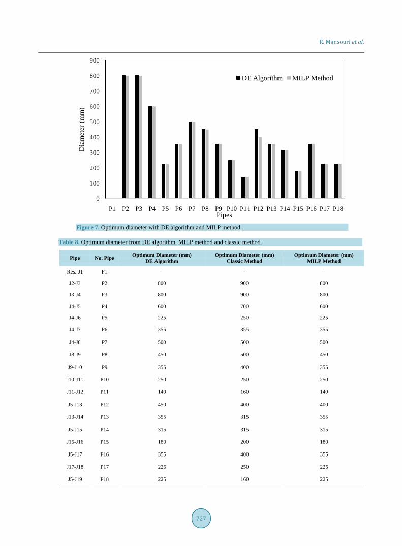
Shahinezhad et al. [30] optimize this network by using mixed integer linear programming method. In this paper the network is optimized by differential evolution algorithm (DE) and the results are compared with absolute optimum that is obtained from mixed integer linear programming (MILP) by Shahinezhad et al. [30]. Table 8 shows the results of optimizing from differential evolution algorithm, MILP and classic method.

In all optimization methods, the factor of time is important. MILP method to find absolute optimum needs more time than DE algorithm, that it’s one of the disadvantages of this method. Although MILP Method achieves the absolute optimum, this method is not recommended in the engineering works that the time is im-portant. The biggest problem in this method is that this method cannot be used in the loop network.

So you cannot use this method to networks that combine the loop and branched network. Figure 7 shows Schematic comparison between optimum diameter of the DE algorithm and MILP method. On the other hand, MILP method is able to solve the tree network and gives absolute optimum, but is unable

to solve loop and complex network (loop and branch). In this study, we compared the algorithm (DE) with this method, Therefore, According to great potential of DE, the algorithm can be used in the loop, branch and com-plex network.

In Table 9 optimal cost obtained by each method can be seen. According to Table 9, it can be said that algorithm presents very good results for optimizing water distribu-

tion network. So that Differential Evolution algorithm estimates cost, 1.57% more than the lowest cost (MILP

R. Mansouri et al.

727

Figure 7. Optimum diameter with DE algorithm and MILP method.

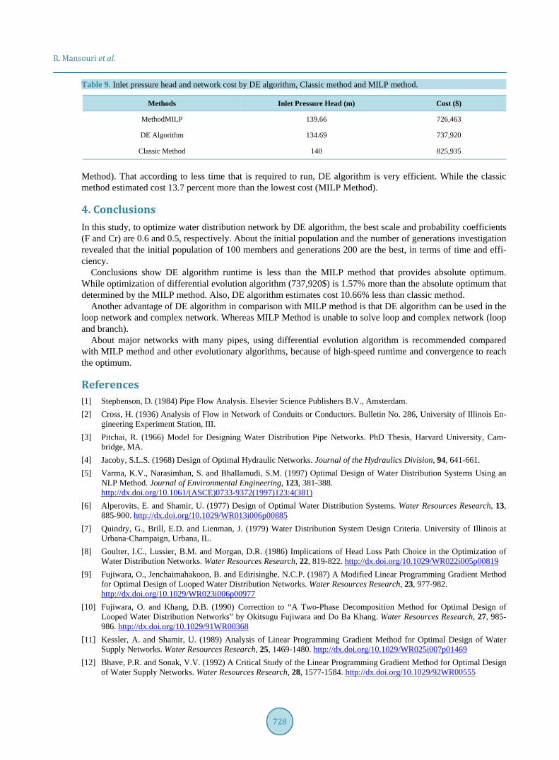
Table 8. Optimum diameter from DE algorithm, MILP method and classic method.

Pipe No. Pipe Optimum Diameter (mm) DE Algorithm

Optimum Diameter (mm) Classic Method

Optimum Diameter (mm) MILP Method

Res.-J1 P1 - - -

J2-J3 P2 800 900 800

J3-J4 P3 800 900 800

J4-J5 P4 600 700 600

J4-J6 P5 225 250 225

J4-J7 P6 355 355 355

J4-J8 P7 500 500 500

J8-J9 P8 450 500 450

J9-J10 P9 355 400 355

J10-J11 P10 250 250 250

J11-J12 P11 140 160 140

J5-J13 P12 450 400 400

J13-J14 P13 355 315 355

J5-J15 P14 315 315 315

J15-J16 P15 180 200 180

J5-J17 P16 355 400 355

J17-J18 P17 225 250 225

J5-J19 P18 225 160 225

0

100

200

300

400

500

600

700

800

900

P1 P2 P3 P4 P5 P6 P7 P8 P9 P10 P11 P12 P13 P14 P15 P16 P17 P18

Dia

met

er (m

m)

Pipes

DE Algorithm MILP Method

R. Mansouri et al.

728

Table 9. Inlet pressure head and network cost by DE algorithm, Classic method and MILP method.

Cost ($) Inlet Pressure Head (m) Methods

726,463 139.66 MethodMILP

737,920 134.69 DE Algorithm

825,935 140 Classic Method

Method). That according to less time that is required to run, DE algorithm is very efficient. While the classic method estimated cost 13.7 percent more than the lowest cost (MILP Method).

4. Conclusions In this study, to optimize water distribution network by DE algorithm, the best scale and probability coefficients (F and Cr) are 0.6 and 0.5, respectively. About the initial population and the number of generations investigation revealed that the initial population of 100 members and generations 200 are the best, in terms of time and effi-ciency.

Conclusions show DE algorithm runtime is less than the MILP method that provides absolute optimum. While optimization of differential evolution algorithm (737,920$) is 1.57% more than the absolute optimum that determined by the MILP method. Also, DE algorithm estimates cost 10.66% less than classic method.

Another advantage of DE algorithm in comparison with MILP method is that DE algorithm can be used in the loop network and complex network. Whereas MILP Method is unable to solve loop and complex network (loop and branch).

About major networks with many pipes, using differential evolution algorithm is recommended compared with MILP method and other evolutionary algorithms, because of high-speed runtime and convergence to reach the optimum.

References [1] Stephenson, D. (1984) Pipe Flow Analysis. Elsevier Science Publishers B.V., Amsterdam. [2] Cross, H. (1936) Analysis of Flow in Network of Conduits or Conductors. Bulletin No. 286, University of Illinois En-

gineering Experiment Station, III. [3] Pitchai, R. (1966) Model for Designing Water Distribution Pipe Networks. PhD Thesis, Harvard University, Cam-

bridge, MA. [4] Jacoby, S.L.S. (1968) Design of Optimal Hydraulic Networks. Journal of the Hydraulics Division, 94, 641-661. [5] Varma, K.V., Narasimhan, S. and Bhallamudi, S.M. (1997) Optimal Design of Water Distribution Systems Using an

NLP Method. Journal of Environmental Engineering, 123, 381-388. http://dx.doi.org/10.1061/(ASCE)0733-9372(1997)123:4(381)

[6] Alperovits, E. and Shamir, U. (1977) Design of Optimal Water Distribution Systems. Water Resources Research, 13, 885-900. http://dx.doi.org/10.1029/WR013i006p00885

[7] Quindry, G., Brill, E.D. and Lienman, J. (1979) Water Distribution System Design Criteria. University of Illinois at Urbana-Champaign, Urbana, IL.

[8] Goulter, I.C., Lussier, B.M. and Morgan, D.R. (1986) Implications of Head Loss Path Choice in the Optimization of Water Distribution Networks. Water Resources Research, 22, 819-822. http://dx.doi.org/10.1029/WR022i005p00819

[9] Fujiwara, O., Jenchaimahakoon, B. and Edirisinghe, N.C.P. (1987) A Modified Linear Programming Gradient Method for Optimal Design of Looped Water Distribution Networks. Water Resources Research, 23, 977-982. http://dx.doi.org/10.1029/WR023i006p00977

[10] Fujiwara, O. and Khang, D.B. (1990) Correction to “A Two-Phase Decomposition Method for Optimal Design of Looped Water Distribution Networks” by Okitsugu Fujiwara and Do Ba Khang. Water Resources Research, 27, 985- 986. http://dx.doi.org/10.1029/91WR00368

[11] Kessler, A. and Shamir, U. (1989) Analysis of Linear Programming Gradient Method for Optimal Design of Water Supply Networks. Water Resources Research, 25, 1469-1480. http://dx.doi.org/10.1029/WR025i007p01469

[12] Bhave, P.R. and Sonak, V.V. (1992) A Critical Study of the Linear Programming Gradient Method for Optimal Design of Water Supply Networks. Water Resources Research, 28, 1577-1584. http://dx.doi.org/10.1029/92WR00555

R. Mansouri et al.

729

[13] Mays, W.L. and Tung, Y.K. (1992) Hydro Systems Engineering and Management. McGraw-Hill, New York. [14] Dandy, G.C., Simpson, A.R. and Murphy, L.J. (1996) An Improved Genetic Algorithm for Pipe Network Optimization.

Water Resources Research, 32, 449-458. http://dx.doi.org/10.1029/95WR02917 [15] Savic, D.A. and Walters, G.A. (1997) Genetic Algorithms for Least Cost Design of Water Distribution Networks.

Journal of Water Resources Planning and Management, 123, 67-77. http://dx.doi.org/10.1061/(ASCE)0733-9496(1997)123:2(67)

[16] Vairavamoorthy, K. and Ali, M. (2005) Pipe Index Vector: A Method to Improve Genetic-Algorithm-Based Pipe Op-timization. Journal of Hydraulic Engineering, 131, 1117-1125. http://dx.doi.org/10.1061/(ASCE)0733-9429(2005)131:12(1117)

[17] Vairavamoorthy, K. and Ali, M. (2000) Optimal Design of Water Distribution Systems Using Genetic Algorithms. Computer-Aided Civil and Infrastructure Engineering, 15, 374-382. http://dx.doi.org/10.1111/0885-9507.00201

[18] Montesinos, P., Guzman, A.G. and Ayuso, J.L. (1999) Water Distribution Network Optimization Using a Modified Genetic Algorithm. Water Resources Research, 35, 3467-3473. http://dx.doi.org/10.1029/1999WR900167

[19] Neelakantan, T.R. and Suribabu, C.R. (2005) Optimal Design of Water Distribution Networks by a Modified Genetic Algorithm. Journal of Civil & Environmental Engineering, 1, 20-34.

[20] Kadu, M.S., Rajesh, G. and Bhave, P.R. (2008) Optimal Design of Water Networks Using a Modified Genetic Algo-rithm with Reduction in Search Space. Journal of Water Resources Planning and Management, 134, 147-160. http://dx.doi.org/10.1061/(ASCE)0733-9496(2008)134:2(147)

[21] Cunha, M. and Sousa, J. (1999) Water Distribution Network Design Optimization: Simulated Annealing Approach. Journal of Water Resources Planning and Management, 125, 215-221. http://dx.doi.org/10.1061/(ASCE)0733-9496(1999)125:4(215)

[22] Eusuff, M.M. and Lansey, K.E. (2003) Optimization of Water Distribution Network Design Using the Shuffled Frog Leaping Algorithm. Journal of Water Resources Planning and Management, 129, 210-225. http://dx.doi.org/10.1061/(ASCE)0733-9496(2003)129:3(210)

[23] Maier, H.R., Simpson, A.R., Zecchin, A.C., Foong, W.K., Phang, K.Y., Seah, H.Y. and Tan, C.L. (2003) Ant Colony Optimization for Design of Water Distribution Systems. Journal of Water Resources Planning and Management, 129, 200-209. http://dx.doi.org/10.1061/(ASCE)0733-9496(2003)129:3(200)

[24] Zecchin, A.C., Maier, H.C., Simpson, A.R., Leonard, M. and Nixon, J.B. (2007) Ant Colony Optimization Applied to Water Distribution System Design: Comparative Study of Five Algorithms. Journal of Water Resources Planning and Management, 133, 87-92. http://dx.doi.org/10.1061/(ASCE)0733-9496(2007)133:1(87)

[25] Ostfeld, A. and Tubaltzev, A. (2008) Ant Colony Optimization for Least Cost Design and Operation of Pumping and Operation of Pumping Water Distribution Systems. Journal of Water Resources Planning and Management, 134, 107-118. http://dx.doi.org/10.1061/(ASCE)0733-9496(2008)134:2(107)

[26] Keedwell, E. and Khu, S.T. (2006) Novel Cellular Automata Approach to Optimal Water Distribution Network Design. Journal of Computing in Civil Engineering, 20, 49-56.

[27] Suribabu, C.R. and Neelakantan, T.R. (2006) Design of Water Distribution Networks Using Particle Swarm Optimiza-tion. Urban Water Journal, 3, 111-120. http://dx.doi.org/10.1080/15730620600855928

[28] Suribabu, C.R. and Neelakantan, T.R. (2006) Particle Swarm Optimization Compared to Other Heuristic Search Tech-niques for Pipe Sizing. Journal of Environmental Informatics, 8, 1-9.

[29] Mansouri, R., Torabi, H. and Mirshahi, D. (2014) Differential Evolution Algorithm (DE) to Estimate the Coefficients of Uniformity of Water Distribution in Sprinkler Irrigation. Scientific Journal of Pure and Applied Sciences, 3, 335- 342.

[30] Shahinezhad, B. (2011) Optimal Design of Water Distribution Networks Using Mixed Integer Linear Programming. PhD Thesis, Shahid Chamran University of Ahvaz, Ahvaz. (In Persian)

[31] Storn, R. and Price, K. (1997) Differential Evolution—A Simple and Efficient Heuristic for Global Optimization over Continuous Spaces. Journal of Global Optimization, 11, 341-359. http://dx.doi.org/10.1023/A:1008202821328

[32] Storn, R. and Price, K. (1995) Differential Evolution—A Simple and Efficient Adaptive Scheme for Global Optimiza-tion over Continuous Spaces. Technical Report, International Computer Science Institute, Berkeley.

[33] Suribabu, C.R. (2010) Differential Evolution Algorithm for Optimal Design of Water Distribution Networks. Journal of Hydroinformatics, 12, 66-82. http://dx.doi.org/10.2166/hydro.2010.014