Embed Size (px)
Citation preview

Faculdade de Ciências e Tecnologia da Universidade de Coimbra
Optimization of the focal plane for the Gamma-Ray Imager mission
Master’s Thesis
João Bernardo Pena Madeira Gouveia de Campos
Supervisor: Doutor Rui Miguel Curado Silva
September 2010


Abstract On April 2004, the European Space Agency (ESA) called for proposals to decide which science themes would have the greatest impact in the future. On 2005, those themes were established and the program Cosmic Vision 2015-2025 was launched. Several missions were proposed within this program to address the different themes. A consortium of several institutions from different countries was formed, and the Gamma--Ray Imager (GRI) mission was proposed. This mission’s aim is to gather information on specific sources of gamma radiation. This work is a small part of the significant effort required for this mission’s development. . The main focus of the present thesis is the main instrument’s sensitivity. From the Compton Gamma Ray Observatory (CGRO) mission in the early 90’s to the International Gamma-Ray Astrophysics Laboratory (INTEGRAL) mission, launched in 2002, the increase in sensitivity was obtained by increasing the photon’s collection area. However, it is no longer possible to increase the sensitivity by enlarging the photon’s collection area. The GRI mission would overcome this problem by making use of Laue lenses, which would focus the incident radiation into the focal plane. Nonetheless, some works allow the supposition that an increase in sensitivity can also be obtained by stacking the detector in several layers. This means that there would be two ways of increasing sensitivity and it is important to quantify which solution would have the greatest impact in the sensitivity’s improvement: the Laue lens or stacking the detector. Various tasks were performed during this work. The first main task performed was the behavior of the signal/noise ratio when different geometries are exposed to different energy distributions. The second main task was testing different geometries corresponding to the same volume divided in a different number of planes; observe how the sensitivity evolves with the increasing number of planes and compare this results with the ones already obtained for Laue lenses. The last main task was the calculation of the Minimum Detectable Polarization (MDP) for the GRI geometry for a beam that suffered the influence of a Laue lens. . All the analysis in this work were performed with the software library Geant4, released by CERN and with MEGAlib, created by Dr. Andreas Zoglauer.


Resumo Em Abril de 2004, a Agência Espacial Europeia (ESA) lançou uma chamada para decidir os temas científicos que teriam maior impacto no futuro. Em 2005, esse conjunto de temas foi estabelecido e deu-se início ao programa Cosmic Vision 2015-2025. Várias missões foram propostas no âmbito deste programa. Um consórcio de várias instituições provenientes de diferentes países formou-se e a missão Gamma-Ray Imager (GRI) foi proposta. O objectivo desta missão é reunir informações sobre fontes específicas de radiação gama. O seu desenvolvimento tem implicado um esforço significativo desde a sua proposta. Este trabalho enquadra-se nesse esforço. A sensibilidade do instrumento principal desta missão é o assunto principal deste trabalho. Desde a missão CGRO (Compton Gamma Ray Observatory), lançada no início da década de 90 do século passado, à missão INTEGRAL (International Gamma-Ray Astrophysics Laboratory), lançada em 2002, o aumento da sensibilidade foi conseguido através do aumento da área de colecção dos fotões. Contudo, já não é possível melhorar a sensibilidade através do aumento da área de colecção. A missão GRI pretende ultrapassar este problema através do uso de lentes de Laue que foquem a radiação incidente num plano focal. No entanto, alguns trabalhos indiciam uma melhoria da sensibilidade através da estratificação do volume activo em várias camadas. Isto significa que poderão existir duas soluções que podem ser usadas para melhorar a sensibilidade e é importante quantificar o impacto de cada uma delas no valor da mesma. A realização deste trabalho passou por um conjunto de tarefas. A primeira foi estudar o comportamento da razão sinal/ruído ao expor diferentes geometrias a diferentes fontes com diferentes distribuições de energia. Seguidamente, estudou-se a variação da sensibilidade com o aumento do número de placas de volume sensível, mantendo constante o volume de detecção, com o fim de comparar os resultados obtidos com o aumento de sensibilidade que se pode esperar através do uso de uma lente de Laue. A última grande tarefa foi o cálculo da polarização mínima detectável (MDP - Minimum Detectable Polarization) para uma geometria simplificada do plano focal a utilizar na missão GRI. Todos os resultados que constam deste trabalho foram obtidos através da livraria de software Geant4, lançada pelo CERN, e do software MEGAlib, criado pelo Dr. Andreas Zoglauer.


Aknowledgements Without Professor Doutor Carlos Alberto Nabais Conde, I would have never met my supervisor and I would have never come to GIAN. This work would not be possible without his intervention.
I would like to thank is my supervisor, Senhor Doutor Rui Silva. He acquainted me with the library software Geant4, without which this work would have never seen light. I also thank him for reviewing different versions of my work, helping me to improve it. I would also like to thank Colin Paul Gloster for his help in dealing with software in front of which I would do little if I was left alone. I would also like to thank Professora Doutora Maria Margarida Ramalho da Costa, Professor Doutor Victor Hugo Rodrigues and Professora Doutora Ana Maria Matos Beja for providing me credible references for the materials’ properties concerning the materials considered in this work. I also owe Dr. Paulo Gomes a debt of gratitude for the different times I asked for his help. He assisted me with software installation and provided me the necessary tools to write this thesis. To Dr.ª Maria Fernanda Fava, Senhora D. Adélia Camarneiro Matos and Senhora D. Rosa Cândida Luís, my warm thanks for their willingness to provide me with the articles I requested, no matter how old they were. Dr. Andreas Zoglauer provided me some hints in how to use the software he created. I am grateful for his assistance. I would like to thank my colleagues, Susana Santos, Inês Ochoa, Edward Santos and Paulo Marques, for making my journey in this department lighter. Finally, I could not forget my family that endured my bad moods. Without their support my task would be much harder to complete. I acknowledge the support given by “Fundação para a Ciência e Tecnologia”, through the project PTDC/CTE-SPA/65803/2006.


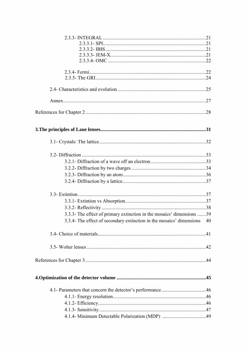
Contents 1.The beginning of a new gamma-ray mission .............................................................. 1
1.1- The Cosmic Vision program .......................................................................... 2
1.1.1- What are the conditions for planet formation and the emergence of life? ............................................................................................................ 2 1.1.2- How does the Solar System work? .................................................. 2 1.1.3- What are the fundamental physical laws of the Universe? .............. 3 1.1.4- How did the Universe originate and what is it made of? ................. 3
1.2- The specific science questions ....................................................................... 4
1.2.1- How do Supernovae explode? ......................................................... 4 1.2.2- What is the origin of the soft gamma-ray cosmic background radiation? .................................................................................................... 4 1.2.3- What links jet ejection to accretion in black hole and neutron star systems? ..................................................................................................... 5 1.2.4- How are particles accelerated to extreme energies in the strong magnetic fields? ......................................................................................... 5
1.3- The mission .................................................................................................... 6
1.3.1- Is it necessary to go to space to observe gamma-rays? ................... 6 1.3.2- What are the mission’s requirements? ............................................. 7
1.4- Organization of the present work ................................................................... 7 References for Chapter 1 ....................................................................................... 9
2.Gamma-ray detection: Materials and Missions ....................................................... 11
2.1 – The Great Struggle ...................................................................................... 12
2.1.1- Crystal scintillators ........................................................................ 12 2.1.2- Gaseous detectors .......................................................................... 13 2.1.3- Semiconductor detectors ................................................................ 14 2.1.4- Coded masks .................................................................................. 15
. 2.2- The different materials ................................................................................. 15
2.2.1- Silicon (Si) ..................................................................................... 15 2.2.2- Germanium (Ge) ............................................................................ 16 2.2.3- Cadmium Telluride (CdTe) ........................................................... 16
2.3- Missions ........................................................................................................ 17
2.3.1- CGRO ............................................................................................ 17 2.3.1.1- BATSE ............................................................................ 17 2.3.1.2- OSSE ............................................................................... 18 2.3.1.3- COMPTEL ...................................................................... 19 2.3.1.4- EGRET ........................................................................... 20
2.3.2- RHESSI ......................................................................................... 20
2.3.3- INTEGRAL ................................................................................... 21
2.3.3.1- SPI ................................................................................... 21 2.3.3.2- IBIS ................................................................................. 21 2.3.3.3- JEM-X ............................................................................. 21 2.3.3.4- OMC ............................................................................... 22
2.3.4- Fermi .............................................................................................. 22
2.3.5- The GRI ......................................................................................... 24 2.4- Characteristics and evolution ....................................................................... 25 Annex ................................................................................................................... 27
References for Chapter 2 ................................................................................................. 28 3.The principles of Laue lenses ..................................................................................... 31
3.1- Crystals: The lattice ...................................................................................... 32 3.2- Diffraction .................................................................................................... 33
3.2.1- Diffraction of a wave off an electron ............................................. 33 3.2.2- Diffraction by two charges ............................................................ 34 3.2.3- Diffraction by an atom ................................................................... 36 3.2.4- Diffraction by a lattice ................................................................... 37
3.3- Extintion ....................................................................................................... 37
3.3.1- Extintion vs Absorption ................................................................. 37 3.3.2- Reflectivity .................................................................................... 38 3.3.3- The effect of primary extinction in the mosaics’ dimensions ....... 39 3.3.4- The effect of secondary extinction in the mosaics’ dimensions 40
3.4- Choice of materials ....................................................................................... 41 3.5- Wolter lenses ................................................................................................ 42
References for Chapter 3 ................................................................................................. 44
4.Optimization of the detector volume ........................................................................ 45
4.1- Parameters that concern the detector’s performance .................................... 46
4.1.1- Energy resolution ........................................................................... 46 4.1.2- Efficiency....................................................................................... 46 4.1.3- Sensitivity ...................................................................................... 47 4.1.4- Minimum Detectable Polarization (MDP) ................................... 49
4.2- Previous simulations on the focal instrument’s optimization .................... 49
4.3- The material’s influence in the detector’s intrinsic efficiency ..................... 51 4.4- Geometry optimization ................................................................................. 54
4.4.1- CdTe detector with decreasing exponential distribution ............... 56 4.4.2- CdTe detector with increasing exponential distribution ................ 58 4.4.3- CdTe detector with uniform distribution ....................................... 61 4.4.4- Si detector with uniform distribution............................................. 63
4.5- Summary ...................................................................................................... 65
References for Chapter 4 ................................................................................................. 67
5.Sensitivity: Comparison between two solutions ....................................................... 69
5.1- Introduction .................................................................................................. 70
5.2- The MEGAlib and event reconstruction ...................................................... 72 5.3- The simulations ............................................................................................ 74 5.4- Background noise ......................................................................................... 75
5.5- Efficiency ..................................................................................................... 79 5.6- Sensitivity ..................................................................................................... 81 5.7- Conclusion .................................................................................................... 83
References for Chapter 5 ................................................................................................. 85
6.Polarimetry.................................................................................................................. 87
6.1 - The Q factor ................................................................................................. 88
6.2 - The Q factor for a specific geometry exposed to monoenergetic sources 89
6.3 - The MDP achieved with Laue lens ............................................................. 92
6.4 - Summary ..................................................................................................... 95 References for Chapter 6 ................................................................................................. 96

7. Conclusions ................................................................................................................. 97
7.1 - Conclusions ................................................................................................. 98 References for Chapter 7 ................................................................................................. 99

Chapter 1
The beginning of a new gamma-ray mission
1

In order to increase European achievements in space, in April 2004, the European Space Agency (ESA) launched a call for different themes concerning many different scientific issues that deserved to be studied. 1.1 - The Cosmic Vision program On 2005 the Cosmic Vision 2015 - 2025 program was launched. Its purpose is to select several scientific missions whose aim is to enlighten four main scientific questions that were based on the themes previously presented. The four questions are: 1 - What are the conditions for planet formation and the emergence of life? 2 - How does the Solar System work? 3 - What are the fundamental physical laws of the Universe? 4 - How did the Universe originate and what is it made of? Each one of these questions covers a wide field of knowledge. The Gamma-Ray Imager mission (GRI) was proposed to ESA in 2007 as an answer to the Cosmic Vision 2015-2025 call and this work can be understood as a contribute to answer questions concerning this mission’s development. 1.1.1 - What are the conditions for planet formation and the emergence of life? The sequential events that give raise to life and the mechanism behind its appearance are still not completely understood. Of course, this cannot be done without clarifying the process that makes gas and dust clouds turn into stars and planets. As life needs a source of energy, only planets orbiting a star are possible candidates for places where life can be found. Nonetheless it is important to find signs of life in their atmospheres and study the habitability in the solar system. Thus, it is important to establish the criteria that make a planet habitable and study in which way the conditions favorable for life appearance and maintenance can change in time. The following issues are presented in [1]. 1.1.2 - How does the Solar System work? The Sun is a fundamental piece of the Solar System. Thus, the way in which our solar system works will never be fully understood if the characteristics of its main star are
2

ignored. Concerning the Sun, the origin of its magnetic field is one of the issues that deserve attention, but also the plasma environment that surrounds it. Another system whose mechanism is still largely ignored is the Jovian System. Its constituents are Jupiter and its moons, and it can be seen as a small model for the solar system. Beyond this aspect, very little is known about the internal structure of gaseous giants, like Jupiter or Saturn. Finally, asteroids and other small bodies deserve attention, since they carry information on the conditions in which the Solar System was born [2]. 1.1.3 - What are the fundamental physical laws of the Universe? Physics is not a complete science. For example, a satisfactory unification theory of all fundamental forces is yet to be found. Thus, it is important to look for deviations from the predictions of the present Standard Model that may give clues for the unified theory so hardly sought. Gravitational waves were predicted by Einstein’s General Relativity Theory and their detection could bring information about black holes, since, according to Hawking’s Theory [5], these objects evaporate by emitting this type of waves. Neutron stars, along with white dwarfs and black holes, are compact objects, whose nature will be explained later (subsection 1.2.4). The first two represent extreme dense form of matter, which could explain some features of matter’s behavior during the first Universe’s moments [3]. 1.1.4 - How did the Universe originate and what is it made of? The current universe theory accepts that the Universe had a period of strong accelerated expansion a very short time after it was formed. It was expected that gravitational forces would make different galaxies closer. However, recent data allows the assumption that the Universe is expanding and different galaxies are becoming distant from each other at an increasing rate. Another purpose of this question is to understand what happened at an early age of the Universe, when first luminous sources were formed and galaxies began to take shape. Finally, the evolving violent Universe requires study. Compact objects, which will be explained later (subsection 1.2.4), phenomena like Supernovae or accretion mass into black holes, are objects and processes that may help to explain the formation of stars and the matter’s behavior at the Universe formation. The Gamma-Ray Imager (GRI) mission was thought to help answering questions related with themes presented in this sub-section and in the previous one. Its purpose is to study the non-thermal Universe [4].
3
1.2 - The specific science questions The GRI mission’s purpose can be summarized in four main themes [6]: 1.2.1 - How do Supernovae explode? Supernovae are violent explosions that expel large amount of matter into the interstellar medium. However, these explosions may have different sources, and, according to the source of the explosion, supernovae are classified according to different classes. Type II supernovae are due to the collapse of regular massive stars (over eight solar masses) [7] once they reach the end of their lives, when thermal pressure due to nucleosynthesis is no longer enough to balance the pressure due to the gravitational force. When a regular light star (less than eight solar masses) collapses it can give rise to a white dwarf. In a binary system it is possible for a white dwarf to accrete matter from a companion star and, in such cases; the Chandrasekhar limit may be crossed. When this happens, there is a thermonuclear explosion: a type Ia supernova. The gamma-rays emitted during this process can give information on the radioactive species produced in these events. For example, it would be interesting to investigate a possible connection between light curves of different supernovae and their explosion mechanism. 1.2.2 - What is the origin of the soft gamma-ray cosmic background radiation? An active galaxy is one that is responsible for the emission of large amounts of energy [8]. It is believed that at the center of these galaxies are supermassive accreting black holes; these are called Active Galactic Nuclei (AGN). The main contribution to Gamma-ray Cosmic Background Radiation (GCBR) is thought to come mainly from them. GCBR is important since its spectral and spatial distributions give information on the origin and growth of stars and galaxies [6]. The energy distribution of the process mentioned above is, to first order, a power law. For present theories, this kind of distribution is due to the inverse Compton scattering of soft photons off hot electrons. The exponent of the distribution and the cut-off energy can give information on the temperature and optical depth of the hot plasma. Thus, these parameters can enlighten the source’s primary emission mechanism, its geometry and the plasma’s physics in the region near it. The determination of these parameters is one of the main objects of the detector in question in this work. Finally, it is believed that violent processes such as accretion of matter onto a supermassive black hole emit polarized photons. If it was possible to measure the degree of polarization, it would be possible to know the angle between the photon’s direction and the disk plane
4

and the optical depth of the emitting region. That is the reason why it is important to build a detector capable of measuring the degree of polarization. 1.2.3 - What links jet ejection to accretion in black hole and neutron star systems? Black holes cannot be observed, but that situation changes if they accrete gas that may have its source in a companion star. The space around rotating black holes is described by the Kerr metric or the Kerr-Newman metric [9], if they also have charge. In this case, the space around the black hole is divided in two places: one outside the ergosphere surface, and one between it and the black hole’s surface. The ergosphere is a region where no stable motion is possible and where jets are accelerated to relativistic energies. Jets are outflows of matter that leave the accretion disk that forms around a black hole. The mechanism by which an outflow of matter comes out of the accretion disk is not clear and gamma-ray observations could give insight on such mechanism. 1.2.4 - How are particles accelerated to extreme energies in the strong magnetic fields? Compact objects can be devised in mainly three groups: white dwarfs, neutron stars and black holes. They represent the collapse of regular stars after nucleosynthesis’ end. White dwarfs are believed to result from the collapse of stars whose mass is less than approximately 8 solar masses, the collapse of stars between approximately 8 and 25 solar masses is believed to originate neutron stars and above this threshold, black holes’ appearance is expected [7]. The mechanism behind white dwarfs and neutron stars is quite complex, but it is possible to state that both represent extreme states of matter. In order for a great system of matter to survive, it is necessary that some kind of pressure balances gravity. In the case of regular stars, the pressure comes from radiation whose origins can be found in nucleosynthesis processes. However, when it comes to compact objects, the balancing pressure comes from particle’s degeneracy pressure, electrons for white dwarfs and neutrons for neutrons stars. In other words, being electrons and neutrons Fermi particles, only two particles with opposite spins can occupy the same phase space, by the Pauli Exclusion Principle. This means that, if a certain gravitational pressure was allowed to be surpassed, particles with the exactly same characteristics would have to occupy the same energy level, and the Pauli Exclusion Principle would be violated. Actually, that threshold can be surpassed; and the result will not be a star, but a black hole instead. Neutron stars can appear alone, spinning around themselves. This type of neutron stars is called “pulsar”. However, pulsars may appear alone or orbiting around another object that may be another pulsar. This is what is called a “binary system”.
5

A magnetar is a highly magnetized neutron star, apparently powered by a huge magnetic field (B>1014G). Such a huge field affects processes like synchrotron emission or Compton scattering. It was observed that these objects emit most of their energy in the soft-gamma ray band. The determination of their spectra more accurately would put constrains on models that explain what happens at such extreme fields. There are also questions about regular pulsars that need answers [6]. One of them is the place where high-energies photons are produced. There are two main models that anticipate where these photons might be produced: the polar cap models assume they are produced in the magnetic pole and the outer gap models, assume they are produced near vacuum gaps in the outer magnetosphere. These two models make different predictions concerning polarization or pulse morphology and thus, accurate measures of the emitted photons might help to eliminate one of these two theories. 1.3 - The mission Once the main purposes of the GRI are explained, it is important to give a brief explanation on the mission itself. 1.3.1 - Is it necessary to go to space to observe gamma-rays? As shown in the following picture, Earth atmosphere is responsible for the absorption of a great part of the gamma radiation that arrives on Earth. That is the reason why the study of the electromagnetic spectra in the keV range and above is associated with development of vehicles capable of going beyond Earth’s atmosphere. It is necessary to reach an altitude greater than 30km to detect photons with energy over 1MeV.
Fig. 1: Absorption of the electromagnetic radiation by the atmosphere [14].
6

However, in space, a telescope is subject to radiation capable of damaging its electrical components. Although it is important to evaluate the impact of this radiation in the telescope’s electrical components, this will not be done in the present work.
Another consequence of the damaging radiation is the detector’s sensitivity loss. As will be seen on Chapter 4, sensitivity worsens with the rise of background. One way to deal with this situation is implementing an active shield that covers the detector. Once the shield detects a background particle, it prevents the detector from measuring the energy depositions for a certain time by marking the data acquired with a veto. 1.3.2 - What are the mission’s requirements? It is important that the mission represents an improvement relatively to its predecessors, namely INTEGRAL [10]. The mission requirements are given in Table 1:
Table 1: The new mission’s requirements [11] Parameter Requirement Goal
Energy band (keV) 20 - 900 10 - 1300 Continuum sensitivity
(ph cm-2s-1keV-1) 10-7 3 x 10⁻⁸
Narrow line sensitivity (ph cm-2s-1) 3 x 10⁻⁶ 10-6
Energy resolution 3% 0.5% Field of view (arcmin) 5 10
Angular resolution (arcsec) 60 30 Time resolution (µs) 100 100
Polarization MDP (for 10 mCrab in 100ks) 5% 1%
As will be seen, one of the main important features of this mission is to enlarge the energy range of its predecessor. One important feature is sensitivity since there is still a great margin for improvement. As stated in [11], one of this mission’s requirements is that its sensitivity is ~30 times better than the one achieved by INTEGRAL (please, see Chapter 2). 1.4 - Organization of the present work Since the first gamma-ray missions in the 60’s [15], several gamma-ray missions have been launched. The most recent ones are presented in the next chapter. In a mission like INTEGRAL (Chapter 2), the area in which photons are collected is the same area used to detect them. The GRI mission will use Laue lenses (Chapter 3) to collect the photons observed into a focal plane. Thus, unlike a mission such as INTEGRAL, in the GRI mission, the 7

decoupling between the collecting area and the detecting area is used as a way to increase sensitivity [13]. The detection area must be designed so that sensitivity achieved is the best possible for a given collecting area. The use of Laue lenses represents a major step in the gamma-ray detection technology. However, in [12] a way to increase sensitivity without the mentioned decoupling is presented. In this reference, slicing the detection volume in several layers is presented as a solution to increase sensitivity. It is important to quantify the sensitivity gain obtained by using this solution and by using the decoupling solution. In Chapter 4 the materials that may allow a better efficiency are studied and the detector’s thickness values’ that allow the best signal/noise ratio are determined. In Chapter 5, I will compare the sensitivity obtained for different detectors sharing the same volume but not the same number of layers. An improvement in the sensitivity’s value is expected. The results obtained are compared to the improvement that may be accomplished by making use of a Laue lens. In Chapter 3 I will present the concept of Laue lenses, since these will be part of the GRI mission and, in Chapter 6, I will present the polarization sensitivity behavior of the geometry proposed for the GRI mission.
8

References for Chapter 1 [1] - http://sci.esa.int/science-e/www/object/index.cfm?fobjectid=38646 [2] - http://sci.esa.int/science-e/www/object/index.cfm?fobjectid=38656 [3] - http://sci.esa.int/science-e/www/object/index.cfm?fobjectid=38657 [4] - http://sci.esa.int/science-e/www/object/index.cfm?fobjectid=38658 [5] - Hawking, S. W., Black holes and thermodynamics, Phys. Rev. D, vol. 13, 2, 191-197 [6] - P.I. Jürgen Knödlseder, “GRI exploring the extremes”, submitted proposal to Cosmic Vision 2015-2025 call for missions, June 2007 [7] - Woosley, S. E., Heger, A., “The evolution and explosion of massive stars”, Rev. Mod. Phys., 74, 1015 (2002) [8] - Kaufmann, W., Freedman, R., “Universe”, 5th edition, W. H. Freeman and Company (1998) [9] - Shapiro, L. S., Teukolsky, S. A., “Black Holes, white dwarfs and neutron stars”, John Wiley & Sons, 1983 [10] - Carli, R. et al.,“The INTEGRAL Spacecraft”, 3rd INTEGRAL Workshop 'The Extreme Universe', Taormina, Italy, 14-18 Sept 1998 [11] - Knödlseder, J., “GRI: The Gamma-Ray Imager mission”, A.S.R., vol. 40, 1263 – 1267 (2007) [12] - Takahashi, T., “A Si/CdTe Compton Camera for gamma-ray lens experiment”, Exp. Astro., vol. 20, 317-331 (2006) [13] - Frontera, F. et al., “Exploring the hard X-/soft gamma-ray continuum spectra with Laue lenses”, Proc. 39th ESLAB Symposium, in press, 2005 (astro-ph/0507175) [14] - Léna, P., “Astrophysique – Méthodes physiques de l’observation”, 2nd edition, InterÉdition/CNRS Éditions (1996) [15] - Meuris, A.,“Étude et optimization du plan de detection de haute énergie en Cd(Zn)Te de la mission spatiale d’astronomie X et gamma Simbol-X”, PhD Thesis (2009)
9


Chapter 2
Gamma-ray detection: Materials and Missions
11
In this chapter I will analyze the gamma-ray telescopes’ evolution in the last years and the technologies used to improve the sensitivity of these devices. In section 2.1 I will present the theoretical principles of the technologies used, in section 2.2 I will present some typical materials used in gamma-ray detection. In section 2.3 I will present some missions that marked the evolution of gamma-ray detection and, in section 2.4 I will present the evolution of sensitivity achieved in different missions. 2.1 - The Great Struggle Many different technologies were applied in order to improve the gamma-ray detectors’ performance. Some of them are crystal scintillators, gaseous detectors, semiconductor detectors and coded masks, although these are not part of the detectors’ family. 2.1.1 - Crystal scintillators As can be noticed in [1], scintillator detectors are a vast field. Thus, I will only consider crystal scintillators since they are the main type of scintillators used in the missions whose description follows. In a crystal, atoms are organized in a regular pattern, which implies a well defined energy band structure. This structure is composed of band energies accessible to electrons separated by energy gaps that cannot be occupied. The two energy bands considered are the valence band, where all electrons would be at a temperature of 0K and the conduction band, which can be occupied if electrons gain enough energy to leave the valence band. These two bands are separated by an energy gap and the reason why they are the only ones considered is that energy bands below the valence band are all occupied and energy bands above the conduction bands are all empty. Thus, the crystal’s conductivity will be determined by the electrons present in the conducting band, the holes left in the valence band and the energy gap. In a crystal scintillator, a particle deposits energy in the material, exciting an electron from the valence band to the conduction band, and, in the de-excitation process, a photon is emitted. However, this process lacks efficiency since the photon emitted would not lie in the visible range. Thus, some atoms that will play the role of impurities called activators are added to the crystal in order to deform the energy band’s structure locally, allowing intermediate energy levels to appear in the forbidden band. In this way, the process is slightly changed. When a particle deposits energy in the material, an electron is excited, leaving a hole in the valence band. The hole will ionize the activator, and, because of the distortion in the energy band structure, the excited electron that will encounter the ionized activator will lose its energy by emitting a photon in the visible range.
12

This is the basic principle behind the scintillation mechanism in inorganic crystals. In the case of NaI(Tl), for example, this means NaI represents the atoms that compose the crystal structure and Tl will be the element that will act as an activator. 2.1.2 - Gaseous detectors The principle behind gaseous detectors is quite simple: a charged particle passes through the gas contained in a chamber and ionizes neutral molecules, originating an ion and an electron per molecule ionized. However, the energy deposited is known due to the charges created by the ionizing particle, and if the generated charges are not collected, there will be no detection. So an electrical field is applied in order to make the electrons generated drift to the anode. If the electrical field is too weak, the charges collected are less than the charges created due to recombination processes. As the applied field increases the recombination events are suppressed and all charges are collected. This is the “ion saturation” region where ion chambers operate. In this case, the energy transmitted by the field to the generated electron by the field is only enough to make it reach the anode. If the electrical field’s value is increased, the generated electron will have enough energy to not only reach the anode, but also ionizing other particles in its way, originating an avalanche. The number of charges collected will be proportional to the charges initially generated. This is the region where proportional counters operate. It is also possible to further increase the field applied, but that would lead to a situation where the number of charges collected is not proportional to the number of charges generated. It is obvious that avalanches will only be produced if the colliding electron has an energy superior to the ionizing energy [1]. In spark chambers, the gas is contained between two conducting plates [3]. When a charged particle crosses the gas, provoking a discharge, a spark arises, marking the particle’s path. There are also hybrid detectors that combine characteristics from proportional counters and scintillators. In this case, the purpose is not to ionize the gas’ molecules, but to excite them, so they emit light by decaying to their ground state [1,2]. The gases usually used for this purpose are noble gases, such as Xenon or Helium. Normally, their emission is in the ultraviolet region. In this situation, photomultiplier tubes sensitive to this emission are used or a process to shift the wavelength is used. This process can be the covering the walls of the container with diphenylstilbene (DPS)
13

[2] or adding another gas, like Nitrogen. The idea is to absorb the ultraviolet photons and emitting light at a longer wavelength [1]. 2.1.3 - Semiconductor detectors According to [1], the scintillation process suffers from serious problems. The most evident is its low energy resolution. The production of one information carrier requires an energy deposition of the order of 100eV, this results in a relatively small amount of charges produced, in the order of tens of thousands, At this point, a clarification should be made. In a metal, the valence band is not fully filled and only electrons will contribute to the conductivity of the material. In a semiconductor, at a temperature of 0 K, the valence band is fully filled, but as the temperature rises, more electrons will pass to the conduction band, leaving holes in the valence band. So, in a semiconductor, electrons and holes will both contribute to conductivity. The only difference between an insulator and a semiconductor is the size of the forbidden band. In an insulator, the energy gap is big enough to ensure that an electron cannot be thermally excited to the conduction band and, as a consequence, no current is allowed to flow in such materials. Semiconductors can be doped with donors, atoms that will increase the number of electrons or acceptors, atoms that will increase the number of holes or both. Generally, for detection purposes, there is a semiconductor doped with donors (type n) coupled to a semiconductor doped with acceptors (type p). This forms a p-n junction. It is important to portrait what happens in this situation. At first, there is no electric field in the coupling region, but this is an unstable situation, since the charges’ concentration is not uniform through the coupling region. Thus, holes migrate to the side which has more electrons and vice-versa and, when this process ends, the charges’ concentration within this region is uniform, but an electrical field is now present. This electrical field will guarantee that charges generated by thermal excitation will leave the coupling region and it also guarantees that, if a particle interacts in this region, the charges generated are due exclusively to the interaction [4]. This coupling region is commonly known as depletion zone and its volume can be modified by the application of an external electric field. It is in the depletion zone that particles will be detected and this explains its importance. The number of charge carriers generated by this process outweighs the number of carriers that would be produced in a scintillation process, allowing an increase in energy resolution.
14

2.1.4 - Coded masks In real conditions, events in a telescope are due to signal and noise. Actually, most of the events are due to noise. In order to partly solve this problem, the instrument is pointed in the direction of the source observed, and then pointed in a direction in which only noise is detected. Then, it is possible to remove the noise from the overall events and extract the signal. A coded mask is a filter placed above a detector, and made of a pseudo-random pattern that allow, or not, radiation to pass [4]. The radiation emitted by the source will create a specific pattern in the detection plane which characterizes its position. In a mathematical sense, it is possible to consider the image of the sky to be a function; the mask will be a known mathematical transform that will give the image of the sky in the detection plane, which is also a known function. Knowing the resulting function and the mathematical transform that originates it, it is possible to recover the original function. This is conceptually more complicated than the first method, but allows the background noise to be measured in the same conditions as the source, making it easier to subtract it from the signal, allowing sensitivity’s increment. 2.2 - The main materials used in gamma-ray detection In this section, the most common materials used in gamma-ray semiconductor detectors are presented. 2.2.1 - Silicon (Si) Si is the 14th element of the periodic table and its crystalline structure is equal to the structure of diamond [21,25]:
Its lattice constant is 5.43Å at 20ºC [21]. The cross-sections for photon interactions are given in the annex given at the end of the chapter for all the materials considered.
Fig. 1: Diamond’s crystalline structure [24]
15

As can be seen in the cross-section graphic presented in annex, in the energy range considered (102keV-103keV), the Compton scattering is much more important than photo-electric absorption. As a consequence, the number of photons that leaves the detector without interacting or leaves only part of their energy in the detector increases. 2.2.2 - Germanium (Ge) The structure of this material is the same as the precedent one (Fig. 1) [21,25]. However, its lattice constant is 5.66Å at 20ºC [21]. Although Compton scattering is the most important interaction in the energy range considered, the photo-electronic absorption cross-section for Ge is higher than the one for Si, as can be seen in the graphics presented in annex. This explains why this material has a better efficiency than the previous one. It is also worth noting that Ge is the material which presents the best energy resolution [11], but needs to be cooled. 2.2.3 - Cadmium Telluride (CdTe) This material has a crystalline structure that equals the Zincblend’s [21,23]: Fig. 2: Diamond’s crystalline structure [23].
Its lattice constant is 6.48Å [21]. The photon cross-section for CdTe (presented in annex) explains why this material can be used as a scatterer for high energies. Until ~400keV, the photo-electric process is the dominant process, but above this energy, the Compton scattering effect prevails.
16

2.3 - Missions In this section I will present four missions that stand as an example of how the technologies above presented were used to increase the sensitivity from the dawn of the last decade of the 20th century to the present. These four examples are: CGRO, RHESSI, INTEGRAL and Fermi. 2.3.1 - CGRO The CGRO [5] stands for Compton Gamma Ray Observatory and was a mission maintained by NASA between April 5, 1991 and June 4, 2000. The satellite was equipped with different types of detectors that allowed it to gather information over a large range of the electromagnetic spectrum: from 30keV to 30GeV. These detectors are BATSE, OSSE, COMPTEL and EGRET. 2.3.1.1 - BATSE The Burst And Transient Spectrometer Experiment (BATSE) [6] is an instrument which is composed of two NaI(Tl) scintillation detectors: one is used for sensitivity and directional response (LAD) and the other is used for energy coverage and energy resolution (SD). The LAD is a scintillation disk with a diameter of 20-inches (~50.8cm) and a thickness of 0.5-inches (~1.27cm) separated of a light collector by a circular layer of quartz. The light collector is responsible for bringing the scintillation light into three photo-multiplier tubes (PMT) each one having a diameter of 5-inches (~12.7cm). Their signals are summed within the detector. The background from charged particles is reduced due to a plastic scintillation detector that acts as an anticoincidence shield in front of the LAD. Inside the light collector is also a thin lead and tin shield responsible for reducing the background due to scattered radiation. This device is sensitive to an energy range that between 20 keV and 1.9 MeV. The SD is a circular uncollimated NaI(Tl) scintillation detector with a diameter of 5-inches and a thickness of 3-inches (~7.62). A photo-multiplier tube is directly connected to the scintillation detection window and its housing has the same lead/tin shield already present is LAD. This device is sensitive to an energy range that between 10 keV and 100 MeV. The satellite carried eight BATSE instruments, one at each corner of the space craft.
17

2.3.1.2 - OSSE The Oriented Scintillation Spectrometer Experiment [7] is an instrument designed to undertake observations in an energy range between 0.05MeV and 10MeV. It is composed of four detectors that have the same internal structure and are almost independent from each other, being synchronized by the central electronics, also responsible for the data acquisition, timing and coordinating pointing directions. These four devices are placed in pairs in parallel axis (Fig. 4). Each of these four devices is composed of two circular scintillation crystals NaI(Tl) and CsI(Na), optically coupled, both having a diameter of 330mm. The NaI(Tl) portion has a thickness of 102mm and the CsI(Na) portion has a thickness of 76mm. The CsI face is linked to seven photomultiplier tubes, each having a diameter of 89mm and directly above the NaI portion is placed a tungsten alloy passive slat collimator which defines the gamma-ray aperture of the detection crystal. A plastic scintillator with 508mm2 and a thickness of 6mm that covers the aperture is used to reject background due to charged particles and is linked to four PMT each having a diameter of 51mm. The collimator and the two crystal portions are surrounded by an annular shield made of NaI(Tl) scintillation crystals that is 349mm long and 85mm thick, divided in four independent segments, each linked to three 51mm-diameter PMT. This annular shield, the plastic scintillator and the CsI(Na) portion of the crystal piece act as an anticoincidence shield for background rejection.
Fig. 3: The BATSE [6].
18

2.3.1.3 - COMPTEL The Compton Telescope (COMPTEL) [8] is an instrument that operates in a range between 0.8MeV and 30MeV. It consists of two detector arrays. Seven cylinders with a diameter of 27.6cm and 8.5cm thick each one linked to eight PMT compose the first array. At a distance of 1.5m below this array it is placed the second one, consisting of 14 cylinders made of NaI(Tl) 7.5cm thick and with a diameter of 28cm. Below this array are found seven PMT. Two domes 1.5cm-thick, made of plastic scintillator NE-110 act as anticoincidence shields. This geometry allows the photon to be scattered in the first layer and absorbed in the second layer, the direction of the incoming photon is calculated easily by applying the Compton formula.
Fig. 4: The OSSE [7].
Fig. 5: The COMPTEL [8].
19

2.3.1.4 - EGRET The Energetic Gamma-Ray Experiment Telescope (EGRET) [9] is sensitive to an energy range from 20MeV to 30GeV. The main devices involved in the composition of this instrument are spark chambers, a NaI(Tl) calorimeter and a plastic scintillator. Two spark chambers, each one mounted on top of a NaI(Tl) calorimeter, surrounded by a plastic scintillator dome, constitute the bulk of the instrument. The upper spark chamber allows the conversion of a photon into electron-positron pair. The lower one allows the trajectories of the particles formed to be followed and provides information on how the energy is shared between them. Thus, the determination of the total energy of the photon will depend heavily on measurements made in the lower calorimeter. The energy resolution can suffer for energies above several GeV and below 100MeV. In the first case, the scintillator does not fully absorb the particle’s energy, thus degrading energy resolution. In the second case, energy can be lost in the spark chamber due to ionization processes.
2.3.2 - RHESSI RHESSI [10] stands for Reuven Ramaty High Energy Solar Spectroscopy Imaging and is a mission maintained by NASA launched on February 5, 2002. The satellite is mainly composed of two parts: the first is an imaging system and the second is the spectroscopy system. The imaging system is made of nine pair grids supported by a grid tray. If there is an X-ray source that is not aligned with the detector’s axis of symmetry, as the detector rotates, the signal will be modulated differently by the nine pair grids. This modulation
Fig. 6: The EGRET instrument [9].
20

is important to separate background from the signal since noise signal will not be modulated. As the patterns generated change with the angle between the source and the detector’s axis of rotation, the modulation will also be used to get information about the source’s position. The Ge detectors consist of nine cylinders with a diameter of 7.1cm and a height of 8.5cm. They are prepared to cover a range that goes from 3keV to 20MeV and are cooled down to 75K due to a cryocooler that uses the Stirling cycle to achieve this purpose. 2.3.3 - INTEGRAL The INTEGRAL (International Gamma-Ray Astrophysics Laboratory) [11] is a mission supported by ESA, launched on October 17, 2002. Its energy range covers the visible light up to photons with 10MeV. In order to do so, the satellite makes use of two main detectors: SPI and IBIS and two secondary ones, which will be presented briefly. 2.3.3.1 - SPI The first of the main detectors is the SPI (Spectrometer on INTEGRAL) [12]. It is a device made of 19 hexagonal Ge detectors cooled to a temperature of 85K, intended to make observation within the energy range of 20keV-8MeV. Its energy resolution is 2.2keV (FWHM) at 1.33MeV. It makes use of a Tungsten mask 1.7m above the detection plane. 2.3.3.2 - IBIS The second main detector is IBIS (Imager on Board INTEGRAL) [13]. This detector makes use of two layers of different materials to perform observations. The first layer is made of 16384 CdTe pixels whose dimensions are 4x4x2mm3 and 9cm below, it’s placed the second layer, made of 4096 9x9x30mm3 CsI pixels. This device is intended to perform observations in the 15keV-10MeV range with a spectral resolution of 9% at 100keV. Like SPI, it has a Tungsten mask 3.2m above the detection plane. 2.3.3.3 - JEM-X The third detector used is JEM-X (Joint European X-Ray Monitor) [14]. It is a double gas camera with a mixture of Xe and methane with a pressure that equals 1.5 of the atmospheric pressure at sea level. It’s prepared to make observations within the range of 3keV-35keV with a resolution of 1.2keV (FWHM) at 10keV.
21
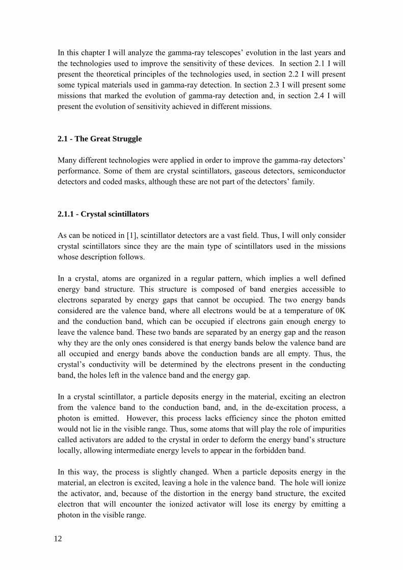
2.3.3.4 - OMC The last detector used in this mission is the OMC (Optical Monitoring Camera) [15] and is conceived to make observations in the range of visible light (500nm-600nm). This device is, in its simplest form, a 5cm diameter lens with a charge-coupled device in its focal plane. Although this detector has 2055x1056 pixels, only 1024x1024 pixels constitute the imaging area. Fig. 7: The INTEGRAL mission payload [16]:
2.3.4 - Fermi The Fermi mission [17] is named after the scientist Enrico Fermi [26] and is a mission launched by NASA on 11th June 2008. It is quite special since it works in the energy range of 20MeV-300GeV and it is, in some sense, the EGRET’s successor [18]. Like this instrument, Fermi’s main instrument is also based on photon-pair conversion, but the principle is quite different. The Fermi’s tracker is made of 16 modules, each one being 37.3cm wide and 66cm high [18]. Each module is made of 18 composite layers made of a tungsten foil, responsible
22

for promoting the conversion photon pair and two Si strips, one responsible for giving the x coordinate and another for the y coordinate. As stated in [18], the tungsten foils are responsible for the conversion of 63% of the normal incident photons. The next figure gives a better visualization of the principle behind the detection:
It is worth noting that, according to [18] the tungsten foils do not have the same thickness. Actually, the first twelve have a thickness of 0.095mm and the next four foils have a thickness of 0.72mm. The last two composite layers do not have a tungsten foil. This happens because it is necessary to find a balance between the maximization of the effective area at high energies and the need to obtain a good Point Spread Function (PSF) at lower energies. The PSF is the probability distribution of the reconstructed direction of an incident gamma-ray. A calorimeter is placed below the tracker. Its purpose is to record the energy deposition of the pair electron-positron, just like in EGRET, and help eliminating background noise. The calorimeter has 16 modules, each having 96 CsI(Tl) crystals (in EGRET, the material used was NaI(Tl)) with a dimension of 2.7cmx2.0cmx32.6cm. Each module is made of 8 layers of 12 crystals each. Both the calorimeter and the tracker are part of the Large Area Telescope (LAT), Fermi’s main instrument.
Fig. 8: A photon entering the Fermi tracker [18].
23

2.3.5 - The GRI The Gamma-Ray Imager (GRI) is the last mission presented. Its concept is still in study and this work is part of the effort to make it a reality. It is important to notice that in traditional gamma-ray telescopes, the area that collects photons is the same that detects them. The INTEGRAL is the maximum exponent of this technique. However, it is not possible to further increase the sensitivity in the energy range 10keV-1.3MeV recurring to this technique due to weight and budget constraints. The idea behind this telescope is to decouple the detection area from the collecting area, by using a focusing system – a Laue lens. In the next chapter the idea behind the focusing system will be explained. The purpose of this section is to expose the main concern of this work: the focal plane. In the proposition submitted to ESA, the focal plane is made of four CZT layers. The first has a thickness of 5mm, to promote photoelectric absorption in the energy range 10keV-250keV, and the other three layers have a thickness of 20mm to allow efficiency better than 75% for photons below 1MeV. The next table presents the characteristics of the four layers taken from [20]:
Table 1
Number of crystals
in each layer Numbers of pixels in
each layer Pixels’ dimensions
First layer 129 33024 0.8 x 0.8 x 5 mm3
Second layer 688 8384 1.6 x 1.6 x 20 mm3
Third layer 688 8384 1.6 x 1.6 x 20 mm3
Fourth layer 688 8384 1.6 x 1.6 x 20 mm3
Fig. 9: The Fermi telescope [17].
24

The next image presents an image of how the satellite GRI will look like: Fig. 10: Na artist view of the GRI mission taken from [19]:
This mission consists in a flight formation of two different spacecrafts: the Optics Spacecraft (OSC), which carries the lenses, and the Detector Spacecraft (DSC), which carries the detector payload [20]. The distance between the lenses and the focal plane is 100m. Theoretically, the axis of both spacecrafts should coincide and the detector area should be parallel to the lens’ surface. In practice it is only possible to know if the axes coincide within ±0.2mm and if the misalignment between the detection area and the lenses is within ±1º. Its orbit will be an ellipse whose perigee is between 15000km and 20000km and its apogee is 183000km. The Earth will be at one focus. This orbit will help to decrease the amount of propellant needed to keep the flight formation and the re-orientation. As a result, the scientific mission can last at least 3 years, plus one for follow-up studies. As this orbit is above the proton radiation belts (10000km high) the material’s activation due to proton bombardment is decreased. 2.4 - Characteristics and evolution The next table presents the characteristics of some devices used in different missions, what type of detectors they are and the magnitude of their sensitivity [6,7,8,9,12,13,14,15]:
´
25

Table 2
Missions’
Instruments Type of detector Energy range
Confidence level (σ)
Sensitivity (cm-2s-1)
CGRO
COMPTEL scintillator 0.8MeV-30MeV
3
6 x 10⁻⁵ (1 MeV)
1.5 x 10⁻⁵ (7 MeV)
EGRET spark chamber/crystal
scintillator 20MeV-30GeV
- 6 x 10⁻⁸
(E > 100 MeV)
OSSE crystal scintillator 0.05MeV-
10MeV -
~10-4
(1MeV)
INTEGRAL
SPI semiconductor
detector 0.02MeV-
8MeV 3
2.8 x 10⁻⁵ (511 keV)
IBIS semiconductor
detector 0.015MeV-
10MeV 3
2.0 x 10⁻⁵ (100 keV)
JEM-X gas chamber 3keV-35keV 3 1.7 x 10⁻⁵ (6 keV)
GLAST LAT semiconductor
detector 20MeV-300GeV
5 3 x 10⁻⁹
(>100 MeV)
GRI DSC semiconductor
detector 20keV-900keV
3 3 x 10⁻⁶
Sensitivity is the minimum flux that allows the counts from the source to be a certain number of times above the standard deviation. The confidence level is this number. Its value could not be traced for EGRET and OSSE. BATSE was not used to observe a permanent source, but gamma-ray bursts. Its sensitivity is measured in erg cm-2 and its value is 3 x 10⁻⁸ ergs/cm2 for a burst lasting 1 second [6].
26

Annex - Cross sections
Legend:
10-1
10010
-6
10-4
10-2
100
102
Photon Energy (MeV)
(cm2/g)
Compton Scattering for Si
Compton Scattering for Ge
Compton Scattering for CdTe
Photo-electric Absorption for Si
Photo-electric Absorption for Ge
Photo-electric Absorption for CdTe
27

References for Chapter 2 [1] - Knoll, G., “Radiation Detector and Measurement” (3rd edition), John Wiley & Sons, 2000 [2] - Leo, W. R., “Techniques for Nuclear and Particle Physics Experiment” (2nd edition), Springer-Verlag, 1994 [3] - R. P. Shutt (editor),"Bubble and Spark Chambers", academic press, vo1. 1, 3-12 (1967) [4] - Meuris, A.,“Étude et optimization du plan de detection de haute énergie en Cd(Zn)Te de la mission spatiale d’astronomie X et gamma Simbol-X”, PhD Thesis (2009) [5] - http://heasarc.gsfc.nasa.gov/docs/cgro/index.html [6] - http://heasarc.gsfc.nasa.gov/docs/cgro/batse/ [7] - http://heasarc.gsfc.nasa.gov/docs/cgro/osse/ [8] - http://heasarc.gsfc.nasa.gov/docs/cgro/comptel/ [9] - http://heasarc.gsfc.nasa.gov/docs/cgro/egret/ [10] - http://hesperia.gsfc.nasa.gov/hessi/ [11] - http://sci.esa.int/science-e/www/area/index.cfm?fareaid=21 [12] - http://sci.esa.int/science-e/www/object/index.cfm?fobjectid=31175&fbodylongid=719 [13] - http://sci.esa.int/science-e/www/object/index.cfm?fobjectid=31175&fbodylongid=720 [14] - http://sci.esa.int/science-e/www/object/index.cfm?fobjectid=31175&fbodylongid=721 [15] -http://sci.esa.int/science-e/www/object/index.cfm?fobjectid=31175&fbodylongid=722 [16] - http://integral.esa.int/Exploded_view.jpg
28

[17] - Atwood W. D. et al., “The Large Area Telescope on the Fermi Gamma-Ray Space Telescope Mission”, ApJ, 697, 1071–1102 (2009) [18] - Atwood W. D. et al., “Design and initial tests of the Tracker-converter of the Gamma-ray Large Area Space Telescope”, Astrop. Phys., 28, 422–434 (2007) [19] - Knödlseder, J., “Prospects in space-based Gamma-Ray Astronomy”, 39th ESLAB symposium (2005) [20] - Knödlseder, J. et al, “GRI: focusing on the evolving violent universe”, Exp. Astron., 23, 121–138 (2009) [21] - Pearson, W. B., “A handbook of Lattice and Structures of Metals and Alloys”, Pergamon Press, reprinted with corrections (1964) [22] - http://www.nist.gov/physlab/data/xcom/index.cfm [23] - http://cst-www.nrl.navy.mil/lattice/struk/b3.html [24] - http://newton.ex.ac.uk/research/qsystems/people/sque/diamond/structure/
[25] - http://cst-www.nrl.navy.mil/lattice/struk/A4.html [26] - http://www-glast.stanford.edu/
29


Chapter 3
The principles of Laue lenses
31

As was mentioned earlier in this work, one way to increase sensitivity is to decouple the sensitive area from the collecting area. In a direct-view telescope, the area where particles impinge is the same area where they deposit their energy. In the GRI mission, Laue lens will be used to focus photons. Thus, it is important to explain what are they and how crystallographic concepts influence their conception. 3.1 - Crystals: The lattice A crystal is characterized by the fact that its atoms are organized in a specific pattern called lattice. Because of this pattern it is always possible to find three vectors a, b, c, so that every point in the lattice can be given by a vector in the form: r ua vb wc, where u,v and w are integers. This pattern allows different planes to be considered, being dhkl the distance between the planes of a single family characterized by a vector G ha kb lc , perpendicular to the planes of the family considered, where h, k and l are the Miller indices. It is important to clarify that:
a · (3.1a)
b · (3.1b)
c · (3.1c)
While the vectors without asterisk characterize the lattice, the vectors that carry it characterize the reciprocal lattice. The Bragg law is given by the following expression 2d sin θ! nλ . Its meaning is quite simple: considering a wave impinging on a lattice, only the waves with a wavelength λ or its multiples will not suffer destructive interference by the plane family (h,k,l), where 2θB is the angle between the direction of the incident wave and the diffracted wave. Bearing this in mind, it is possible to explain what a Laue lens is. The Laue lens is an assemblage of small crystals. But this assemblage is not random. If all the planes (h,k,l) in each small crystal made the same angle with the direction of the incident beam, this would mean, according to Bragg law, that only one value of energy would be focused at the chosen point. But if these small crystals are slightly misaligned, the energy range refracted into a focal plane will increase. As a consequence of the Bragg law, the more significant the misalignment is, the larger the energy range the lens can refract is, but the area in the focal plane in which they will refract the photons will also increase.
32

This was a first approach in order to make the basic principles of a Laue lenses more evident. In the next section, the diffraction of photons will be considered in more detail and the extinction phenomenon will be explained in order to understand the limits required on the small crystals’ dimensions. 3.2 - Diffraction The main purpose of this section is to study the diffraction of a wave or, in order words, the mechanism behind Laue lenses. This study will follow a specific order: the diffraction off an electron, an atom and a crystal lattice. 3.2.1 - Diffraction of a wave off an electron An electromagnetic wave travelling along the x axis with the electric field along the z axis can be described by the expression: E$r, t& E'e)$·*+,-&e./ (3.2) An electron that suffers the influence of such a field will radiate according to the following equations [1]: B µ'H (3.3)
H 3456789: $r. p& < B =µ>
?>34567
89: $r. p& (3.4)
E 3456789?>: $r. p& r. (3.5)
Considering a charge at the origin of a coordinate system, the fields E and B will be the electric and magnetic field emitted by the oscillating charge at a distant point given by the vector r, fig. 3.1. The vector p is the dipole vector of the oscillating charge:
Fig. 1: Dipole radiation (after [1]).
33

Finally, through the Pointing vector S A!Bµ> it is possible to obtain the expression for
the intensity diffracted [1]:
ID I' E F389?>GH3:IB $$sin J&B $cos J&B$cos θ&B& (3.6)
If the beam in question is not polarized, an average over the angle J must be made, resulting in the expression:
ID I' E F389?>GH3:IB ELM$NO P&3
B I (3.7)
This last expression will be the intensity diffracted by a single electron. 3.2.2 - Diffraction by two charges The treatment given here is in [2]. The expression
φ$r, t& RST:+:′T e)UV·U:+:′W+,-WXYZ[\S (3.8)
can be used to describe the strength of the electric field emitted by a charge exposed to an electromagnetic wave. This expression is an approximation valid only for large distances. It tells what a detector in a position given by r “sees” when the scattering particle is at a position r ′. The factor XYZ[\S is due to the fact that the strength of the field emitted must take into account the strength of the incident wave at the particle’s position. It is worth noting that this phase difference will depend in k), the wave vector before scattering and r ′, the atom’s position. This means that the phase introduced in the emitted wave will depend only on proprieties of the wave before the interaction and on the crystal structure, something that makes sense. The diffraction pattern of two emitting particles at positions rL and rB, is the sum of two waves given by the expression above. The value of Tr ] rL′ T is close to Tr ] rB′ T, since both particles will be far from the detector. Although, a slight variation of this value will not change significantly the wave’s amplitude, it will have a strong impact in the exponent. After some calculations and taking into account eq. 3.8, it is possible to obtain the waves emitted by particles 1 and 2:
34

φL$r, t& Ae)UV·:+,-WX+Y∆Z\S (3.9) φB$r, t& Ae)UV·:+,-WX+Y∆Z\3S (3.10) ∆a ab ] aY (3.11) The wave corresponding to the wave scattered by two neighboring atoms in two different positions rL and rB is represented by equations 3.12 and 3.13: cd cL cB (3.12)
cd eXYUZf·\+gdW hX+Y∆Z·\′ X+Y∆Z·\3′ i (3.13) The following picture illustrates the situation: Making all the calculations, the intensity will be given by:
cdcd 4|e|B Ecos hLB ∆a · $lL ] lB&iIB
(3.14) From this equation, it is possible to deduce the Bragg law. This law is obtained considering that a maximum of intensity will be obtained only if LB ∆a · $lL ] lB& mn < ∆a · $lL ] lB& 2mn; m p q (3.15) The vectors ab and aY are the wave vectors of the diffracted and incident wave respectively, λ is the wavelength. Considering that the distance between two neighboring atoms of different planes is:
Fig. 2: The vectors rB and rL represent the point charges’ positions. The vectors krB and k)B represent the final and initial wave vectors of the second wave (φB). The vectors krL and k)L are the equivalent vectors for the first wave (φL).
35

d |rL ] rB| (3.16) And the following:
U∆kWB Ukr]k)WB (3.17)
TkrT Tk)T B9
s (3.18) It is easy to conclude that:
U∆kWB EB9s IB $1 ] cos 2θ!& (3.19)
Where the angle 2θ! is the angle between the incident and diffracted directions. The final result will be: T∆kT B9
s sin θ! (3.20) Squaring equation 3.19, the Bragg law is obtained: 2d sin θ nλ (3.21) Where θB is the Bragg angle. This angle corresponds to half of the angle between the incident and diffracted directions for which the intensity is maximal. 3.2.3 - Diffraction by an atom This section will be a short one. However it implies a conceptual jump. In the last section the expression for a wave diffracted by two charges was obtained:
φ- Ae)UV·:+,-W he+)∆·:` e+)∆·:3i (3.22) How will this expression change for a cloud of charges? It is a matter of summing different wavelets diffracted by charges at a distance r) from the nucleus [2]: φ- Ae)UV·:+,-W ∑ e+)∆·:5v)wL (3.23) But, in the atomic cloud, the charges can be distributed according to a certain density n$r&, so the sum can be replaced by an integral: φ- Ae)UV·:+,-W x n$r&e+)∆·:5y
' dV (3.24)
36

The form factor is: f)U∆kW x n$r&e+)∆·:5y
' dV (3.25) This factor depends on the atom in question. The form factor, which expresses the influence of an atom on an incident wave, is different for a germanium atom or a copper atom. 3.2.4 - Diffraction by a lattice To obtain the effect of a lattice on an impinging wave, the procedure of expression 3.23 is applied. Knowing that an atom has a position r) in the lattice and knowing its form factor fi, it is possible to write, applying the same method used previously: φ- Ae)UV·:+,-W ∑ f)e+)∆·:5|)wL (3.26) This last expression is the resulting wave diffracted by the crystal. It is important to mention that F ∑ f)e+)∆·:5|)wL (3.27). The form factor will depend on the Miller indices since (see section 3.1): ∆k G (3.28) 3.3 - Extintion In the last section I considered the mechanism of diffraction. At this moment one parameter must be considered: reflectivity. The concepts of primary and secondary extinction and absorption should also be examined. The reason for considering these different aspects is related to the fact that they will define the size of the small crystals that make the lens. 3.3.1 - Extintion and Absorption This section is based on the Darwin’s papers that first gave a mathematical model for the extinction process [3,4,5] and on [6]. If a beam impinges on a crystal it will lose some of its energy after having crossed the sample. It is possible to imagine that the sample consists of a perfect crystal, which occupies its entire volume. The interference
37

of the incident beam within the sample will be responsible for the loss of part of the beam’s energy. This phenomenon is called primary extinction. On the other hand, it is possible to imagine that the sample is made of little small domains having each one a well organized lattice. In this case, the sample is considered as ideally imperfect. However, each of these domains will be responsible for diffracting parts of the incident beam in different directions. This will, of course, decrease the beam’s intensity when it leaves the sample. This phenomenon is called secondary extinction. Normally a true sample does not behave like an ideally perfect or imperfect crystal. Its behavior will be something between these two extreme cases. If the main objective is to study the material’s properties, some corrections must be applied to the diffracted pattern obtained. Although these correction factors are important is solid state physics, this is not the purpose of this work. What I intend to show is how primary and secondary extinction will be used to determine the size of the crystals that are used to build the lens. There is also the absorption process that will contribute to the loss of energy from the impinging beam. Absorption can be due to photoelectric effect or Compton scattering [7]. In the photoelectric effect, the photon is absorbed by an atom, and an electron is emitted. In the Compton scattering, a photon of the incident beam changes its direction, but unlike in the diffraction case, this change in direction is completely independent of the material’s structure or organization. These effects must be taken into account when considering the dimensions of the crystals that will be used to make the lens. 3.3.2 - Reflectivity Integrated reflectivity is given by [1]:
R x $A,P&6>$A&
PP5 dθ (3.29)
The meaning of this expression is quite simple: P'$E& is the power of the incident beam, and P$E, θ& is the power diffracted in a direction given by θ by a plane family identified by the Miller indices (h,k,l). This is not a contradiction since the Bragg law was derived assuming the maximal’s positions of the diffraction’s pattern (eq. 3.15), but this maximum is in fact a peak, and it makes sense to consider that the intensity diffracted is important over a small rangeθ! ] ∆θ, θ! ∆θ .
38

3.3.3 - The effect of primary extinction in the mosaics’ dimensions In this section it will be seen how the primary extinction affects the dimensions of the mosaic crystals that compose the lens. According to [1,8], the expression given for reflectivity must be corrected when primary extinction is important. In the present case, the reflectivity is:
R′ f$A& · R < R′ f$A& x $A,P&6>$A&
PP5 dθ (3.30)
Where R is the maximum integrated reflectivity a crystal can have. The values of f(A) and A are given below:
f$A& - RM|NO BP| -|R NO BP|R$LM$NO BP&3& (3.31)
A :Hsy |F| -
NO P> (3.32)
Where r4, the classical electron radius, is ~2.82x10⁻⁵ (Å), λ is is the wavelength of the photon, |F| is the structure factor, t is the mosaic’s thickness, θ' is the angle between the incident direction and the normal of the plane’s surface and V is the volume of the lattice’s cell. The following graphic shows the function f$A& as a function of A for different values of |cos 2θ!|:
Graphic 1: f$A& is represented on the y axis and, on the x axis, is represented e. This graphic was built using Matlab [13].
0 0.1 0.2 0.3 0.4 0.5 0.6 0.7 0.8 0.9 10.75
0.8
0.85
0.9
0.95
1
A
f(A)
f(A) vs A|cos(2theta)|=0|cos(2theta)|=0.1
|cos(2theta)|=0.2|cos(2theta)|=0.3|cos(2theta)|=0.4
|cos(2theta)|=0.5|cos(2theta)|=0.6|cos(2theta)|=0.7
|cos(2theta)|=0.8|cos(2theta)|=0.9
39
As can be seen, when the value of A tends to zero, the value of f$A& tends to unity. This means that the lower the value of A is, the lesser will be the influence of primary extinction in the integrated reflectivity. So, the upper bound for mosaic thickness is given by: e 1 \
|Z| dNO > 1 NO >
\|| (3.33)
3.3.4 - The effect of secondary extinction in the mosaics’ dimensions Considering a crystal with its perfect domains slightly misaligned around a specific angle with a distribution that follows a Gauss law:
W$∆& L√B9 e+ ∆3
33 (3.34)
The mean reflectivity of a single layer of the crystal will be [1,7]:
x W$∆& 6>
$θ ] θ! ] ∆&d∆ W$θ! ] θ&R (3.35)
R is the integrated reflectivity of a single block. The reflecting power of a layer with thickness dT is given by: σdT W$θ! ] θ& 6
- dT (3.36) Where t is the mean thickness of the mosaics and σ the power reflected per thickness unit. In fact this is nothing more than the mean reflectivity of one mosaic times the number of mosaics crossed by the beam. The next step is to consider that, in this geometry; the incident beam will impinge on the crystal in a surface perpendicular to the crystal’s planes. This type of situation is called Laue geometry. The equations that give the power diffracted (Phkl) and the incident power (P0) are: D>D¡ ] µ>>
NO P> ] σP' σP (3.37)
D6
D¡ ] µ>6NO P6
] σP σP' (3.38)
The first term of the second member of both equations represents the part of the beam that was absorbed. The second term, the part of the energy lost to the other beam and
40
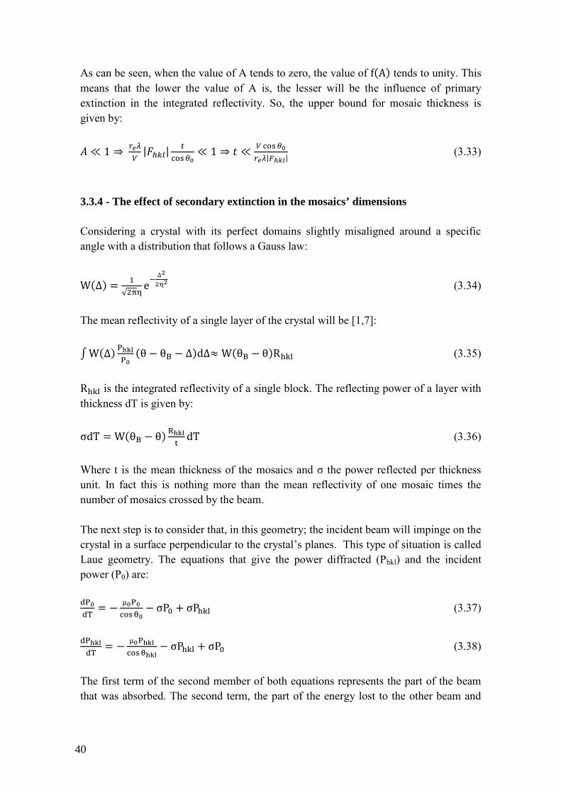
the third is the energy gained to the other beam. The following figure presents both beams impinging on a mosaic:
By solving these equations and considering that the boundary conditions are P'$T& P'$0& at T=0 and P$T& 0 at T=0, it is possible to write: 6$¡>&
>$'& sinh$σT'&e+E µ>£¤¥ ¦>M§I¡> (3.39)
For the lens’ purpose it is important that the power diffracted is the greatest possible. The exponent of this expression can be rewritten as:
] E1 § NO P>µ> I ¡>
µ> £¤¥ ¦> (3.40)
The extinction must be small compared to absorption. This implies: § NO P>
µ> 1 W 6-
NO P>µ> 1 6
µ> t (3.41)
From this section and from the last section it is possible to conclude that: 6
µ> t y NO P>:Hs|¨6| (3.42)
3.4 - Choice of materials The material used to build the lenses must be carefully chosen. It must be easy to find on the market and grown in the right amounts for the purposes in question .They should also have a mosaic configuration [7].
Fig. 3: Na incident beam impinging on a mosaic (after [7]).
41

The material of interest should have a high cell volume. This would result in the decrease in parameter A, thus diminishing the impact of primary extinction over the lens’ performance. Copper and Germanium are well suited for the purpose in question, Highly Oriented Pyrolytic Graphite was also considered, but it was dismissed since technical difficulties prevented mosaic crystals to be properly oriented [9]. The following picture, taken from [7] helps to visualize the idea behind a Laue lens:
´ 3.5 - Wolter lenses Wolter lenses were first described in two articles by Hans Wolter in 1952 [11,12]. This focusing configuration is made with two conic surfaces a parabolic and a hyperbolic surface that are assembled in such way that they share a focal point. The mirror radius, the focal distance and the incident angle are related by the equation: tan 4θ
r . If the incident angle becomes larger than a certain value of θ depending on the beam’s energy, the mirror’s ability to diffract it will fall off quickly. The angle at which a beam is no longer reflected (θ) depends on the material’s density (ρ) and on its energy (E) [10]:
θ © ª«A (3.43)
It is also possible to show that the collecting area of a Wolter I mirror is[10]: AN πηB$f sin 4θ&B (3.44) Where η is the mirror’s reflectivity. The next image presents a scheme of the Wolter I lens:
Fig. 4: The Laue lens.
42

Fig. 5: This image, adapted from [10], is intended to show the Wolter mirror’s focusing principle.
43

References for Chapter 3 [1] - Zachariasen, W. H., "Theory of X-ray diffraction in crystals", Dover Publications, 2004 [2] - Christman, J. R., “Fundamentals of solid state physics”, John Wiley & Sons, 1988 [3] - Darwin, C. G., “The Theory of X-Ray Reflection”, Phil. Mag., series 6, vol. 27, Issue 158, 315-333 (1914) [4] - Darwin, C. G., “The Theory of X-Ray Reflection. Part I”, Phil. Mag., series 6, vol. 27, Issue 158, 675-690 (1914) [5] - Darwin, C. G., “The Theory of X-Ray Reflection. Part II”, Phil. Mag., series 6, vol. 43, Issue 257, 800-829 (1922) [6] - James, R. W., "The optical principles of the diffraction of X-rays", Ox Bow Press, 1962 [7] - Pisa, A.,"Hard X–ray Optics Development: Feasibility Study of a Laue Lens", PhD Thesis, 2004 [8] - De Chiara, P., Frontera, F., "Bragg diffraction technique for the concentration of hard x-rays for space astronomy", Appl. Opt., Vol. 31, nº 10, 1361-1369 (1992) [9] - Pisa, A., e tal., “Feasibility study of a Laue lens for hard X–rays for space astronomy”, arXiv:astro-ph/0411574v2 [10] - Meuris, A.,“Étude et optimization du plan de detection de haute énergie en Cd(Zn)Te de la mission spatiale d’astronomie X et gamma Simbol-X”, PhD Thesis (2009) [11] - Wolter H, “Spiegelsysteme streifenden Einfalls als abbildende Optiken für Röntgenstrahlen”, Annalen der Physik, vol. 10, 94–114 (1952) [12] - Wolter H, “Verallgemeinerte Schwarzschildsche Spiegelsysteme streifender Reflexion als Optiken für Röntgenstrahlen”, Annalen der Physik, vol. 10, 286–295 (1952)
[13] - MATHWORKS, INC. MATLAB user’s guide. Natick, Mass.: MathWorks, Inc., 2010
44

Chapter 4
Optimization of the detector volume
45
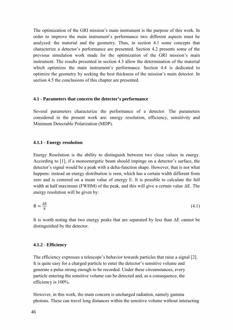
The optimization of the GRI mission’s main instrument is the purpose of this work. In order to improve the main instrument’s performance two different aspects must be analyzed: the material and the geometry. Thus, in section 4.1 some concepts that characterize a detector’s performance are presented. Section 4.2 presents some of the previous simulation work made for the optimization of the GRI mission’s main instrument. The results presented in section 4.3 allow the determination of the material which optimizes the main instrument’s performance. Section 4.4 is dedicated to optimize the geometry by seeking the best thickness of the mission’s main detector. In section 4.5 the conclusions of this chapter are presented.
4.1 - Parameters that concern the detector’s performance
Several parameters characterize the performance of a detector. The parameters considered in the present work are: energy resolution, efficiency, sensitivity and Minimum Detectable Polarization (MDP). 4.1.1 - Energy resolution Energy Resolution is the ability to distinguish between two close values in energy. According to [1], if a monoenergetic beam should impinge on a detector’s surface, the detector’s signal would be a peak with a delta-function shape. However, that is not what happens: instead an energy distribution is seen, which has a certain width different from zero and is centered on a mean value of energy E. It is possible to calculate the full width at half maximum (FWHM) of the peak, and this will give a certain value ∆E. The energy resolution will be given by: R
(4.1) It is worth noting that two energy peaks that are separated by less than ∆E cannot be distinguished by the detector. 4.1.2 - Efficiency The efficiency expresses a telescope’s behavior towards particles that raise a signal [2]. It is quite easy for a charged particle to enter the detector’s sensitive volume and generate a pulse strong enough to be recorded. Under these circumstances, every particle entering the sensitive volume can be detected and, as a consequence, the efficiency is 100%. However, in this work, the main concern is uncharged radiation, namely gamma photons. These can travel long distances within the sensitive volume without interacting
46

and consequently, without generating a pulse. In this case efficiency would be the parameter used to relate the number of particles detected in the sensitive volume to the number of particles impinging on it. This parameter is not uniquely defined. There is an absolute efficiency, defined by equation 4.2 and an intrinsic efficiency, defined by equation 4.3.
(4.2)
(4.3)
Through the rest of the work the word efficiency will be used to refer to intrinsic efficiency, since this will be the parameter I am concerned with. 4.1.3 - Sensitivity At a first approach, sensitivity can be defined as the minimum flux a source must have in order to be detected with a certain level of confidence. The following derivation can be found in [3] and it helps to clarify this concept. Considering a telescope with a collecting area Ad, a background flux B in counts/cm2/s, an observation time t in seconds, a detection efficiency d and a source that has a flux F, given in the same units as B, it is possible to calculate the number of events on the detector due to background noise (N) and due to the source (N): N FAt (4.4) N BAt (4.5) But it is impossible at a first look to separate these two quantities. The signal obtained is: N N ! N (4.6) So, N can be written as: N "N ! N# $ N (4.7) The reason for this is that, although it is not possible to isolate the signal from the background, it is possible to point the detector towards a region where only background noise can be observed. The standard deviation will be:
47

∆N &∆"N ! N#' ! ∆N'()* (4.8)
At this point some assumptions must be made, F and B are not correlated and variations in B are small compared to statistical fluctuations. Finally, when background noise is much greater than the signal, F ++ ,, which is realistic since in the energy range in question (100keV - 1000keV) the signal/noise ratio is about 1:300. Thus, the major contribution to the error comes from fluctuations in B: ∆N √2∆N /2N /2BAt (4.9) Since the uncertainty is given by Poissonian statistics, ∆N √N (4.10) At this moment, it possible to state a minimum detectable flux Fmin. This minimum detectable flux will be the flux that will allow N to be a certain number S above the standard deviation. This means: S 12
∆12 (4.11)
Replacing the values found for Ns and ∆Ns it is possible to obtain the value of sensitivity:
3456 789 : ';
<9= (4.12)
Now that the principle behind sensitivity is explained, it is time to introduce a different situation. In the previous case, it was accepted that the collecting area would be the same as the detecting area. This is not the case for a focusing telescope. For a focusing telescope, the expression for the events generated by the background is the same as in the previous case. However, the value of N changes: N FAt (4.13) In this situation the value of is the fraction of photons that are focused by the optical system and A is its effective area. The demonstration above remains the same for the expression of ∆N, but Ns is now different. This results in a different expression for the sensitivity:
F >?@?ABCAA
:'B@ (4.14)
48

In this case, the value of sensitivity depends on DEFFGH . In the case of a direct-view telescope, sensitivity decreases only with DIGJ.L. This leads to the conclusion that a focusing system will improve a detector’s sensitivity. As it was noticed earlier, there was an attempt from CGRO to INTEGRAL to lower the value of Fmin by increasing the detector’s area. However, that strategy is at its limits due to weight and budget constraints. Nowadays, there are two solutions envisaged to increase sensitivity, which is the same as lowering the flux Fmin: one is presented in [4] and it consists on slicing a detector’s volume in various layers the other is to use Laue lens [5]. 4.1.4 - Minimum Detectable Polarization (MDP) The minimum detectable polarization is the minimum polarization degree a beam must have in order to be recognized as a polarized beam. Its expression is [9]:
MDP 4.29QRs :Rs!RBT (4.15)
Where Q is the modulation factor for a 100% polarized beam. The signal and background count rates RS and RB are in counts/s. As stated in [15], for a pixilated detector, Q 1UG1||
1UW1|| (4.16)
The parameters N|| and NX represent the number of integrated counts in two orthogonal directions for an impinging beam with a polarization degree of 100%. 4.2 - Previous simulations on the focal instrument’s optimization Some simulation work concerning the optimization of the GRI mission’s main instrument has already been done. In [8] five different geometries have been considered and compared in terms of sensitivity and in [11] a polarimeter’s behavior is tested. The purpose of the works considered was to test the behavior of finished configurations. The results obtained would not change the detectors tested. That is particularly true for the experiment presented in [11]. This work’s purpose is to optimize a geometry that is not yet a reality. The following paragraphs concern the work presented in [8]. Geometry 1 corresponds to a stacked detector of 6 CZT layers. Each one is made of 6 x 6 crystals, each having a dimension of 20 x 20 x 7 mm3 divided by 10 x 10 pixels.
49

The energy resolution of a single layer is 9.6keV (FWHM) at 662keV at the first layer and it raises to 19.2keV at the detector’s bottom. The same happens with the trigger threshold: 10keV at the top layer 40keV at the last. The shield is made of BGO and its thickness is 5cm at the bottom and 2cm on the sides. Its trigger threshold is 70keV. The shield’s entry window is covered by a plastic scintillator, whose thickness is 0.95cm and its trigger threshold is 200keV. The detector corresponding to geometry 2 is equal to the previous one in every aspect, except that it has five collimators in front of its window. Their purpose is to protect the detector against lower-energy cosmic photons. Each collimator is made of 0.9cm lead, 0.2cm cadmium and 0.04cm copper. The detector corresponding to geometry 3 is a stacked detector has 35 layers of double-sided silicon-strip detectors, their dimensions are: 100 x 100 x 1.5 mm3. Under these, there are 10 CZT layers. 4 layers of this material surround the detector. The BGO shield and the plastic scintillator have the same characteristics as in the previous detectors. The detectors corresponding to geometries 4 and 5 have the same characteristics: they both have an energy resolution of 1.5keV FWHM at 662keV, a noise threshold of 8keV and a trigger threshold of 15keV. They don’t have any active shield. Geometry 4 is made of 4 Ge Crystals whose dimensions are 80 x 80 x 15 mm2 and a 2mm strip pitch. Geometry 5 consists of 12 crystals whose dimensions are 130 x 70 x 17.5 mm3 and a 1mm strip pitch. The results are presented in the following graphic:
Graphic 1: Sensitivity for geometries studied in [8].
50

Geometry 3 presents the best sensitivity for most of the energy range. This allows the conclusion that the use of Si for the GRI main instrument’s payload may help to improve sensitivity. Another work concerns the performance’s improvement in what concerns polarimetry. CIPHER (Coded Imager and Polarimeter for High Energy Radiation) is a detector described in [11] designed to perform polarimetric measurements. Its energy range covers the values from 100keV to 1000keV. This detector is made of 4 modules placed in two pairs side by side. None of the 4 modules is symmetrical. Each of the 4 modules is made of 32 linear modules, which are 0.5mm thick Al2O3 parallel planes, separated by 3mm. Each plane gives support to a row of 32 pixels separated by 0.1mm aligned in a direction perpendicular to the direction defined by the planes’ normal vector. The pixels have a squared surface (2 x 2 mm2), a thickness of 10mm and are made of CdTe. In each module, the path between two pixels is different in the two orthogonal directions. Because of this fact, the placement of the 4 modules was made in such a way that they were rotated 90º in relation to their nearest neighbor. Each module was irradiated with the same beam and the double events obtained in each module were summed in a 32x32 matrix. This method takes into account the rotation of the modules. This study validates the rotation technique to correct the asymmetry and Q values above 0.5 were obtained between 200keV and 400keV. This geometry proved to be better than the one used for the GIPSI polarimeter [12], since although a Q factor of 0.7 can be obtained, its energy range is much narrower (70keV - 300keV). The geometry used on the INTEGRAL mission allows a much wider energy range than CIPHER (200keV - 3MeV) but the Q factor is lower than 0.3 [13]. 4.3 - The material’s influence in the detector’s intrinsic efficiency Using the toolkit simulation [6], I considered two situations: a detector having a shape of a plate with dimensions of 128x128x5mm3 and another with 128x128x10mm3. For each of these situations, I considered three typical materials used on gamma-ray detectors for satellite missions: Ge (germanium), Si (silicon) and CdTe (cadmium telluride). In my work I restricted myself to the case of perfect charge collection. The detector samples were irradiated with a circle shaped source with 0.5 mm radius and whose radius center coincides with the sample’s surface center. As the samples sizes’ are 128mm, the source can be considered point-like.
51

The results obtained are contained in the following tables. The main point of this section is to confirm which material is best suited to increase the detector’s efficiency. It is important to notice that P.I. stands for Photons that Interacted, which means photons that left part or all of their energy within the detector, P.T stands for Photons that left their Total energy within the detector and i. efficiency stands for intrinsic efficiency. The symbol σ represents the estimated error:
Table 1
Ge 5mm thickness plate E(keV) P.I. σP.I. P.T. σP.T. i. efficiency σi.eff.
100 369800 608 344105 587 0.931 0.002 400 106083 326 21305 146 0.201 0.002 700 83190 288 8191 91 0.098 0.001
1000 70134 265 4852 70 0.069 0.001
Table 2
Ge 10mm thickness plate E(keV) P. I. σP.I. P. T. σP.T. i. efficiency σi.eff.
100 232862 483 224300 474 0.963 0.003 400 94610 308 29115 171 0.308 0.002 700 75827 275 13637 117 0.180 0.002
1000 65360 256 8803 94 0.135 0.002
Table 3
Si 5mm thickness plate E(keV) P.I. σP.I. P.T. σP.T. i. efficiency σi.eff.
100 106160 326 22665 151 0.213 0.002 400 62839 251 504 22 0.0080 0.0004 700 84337 290 265 16 0.0031 0.0002
1000 358908 599 812 28 0.0023 0.0001
Table 4 Si 10mm thickness plate
E(keV) P.I. σP.I. P.T. σP.T. i. efficiency σi.eff. 100 193171 440 52734 230 0.273 0.001 400 119478 346 1857 43 0.0155 0.0004 700 96614 311 635 25 0.0066 0.0003
1000 82999 288 383 20 0.0046 0.0002
52

Table 5 CdTe 5mm thickness plate
E(keV) P.I. σP.I. P.T. σP.T. i. efficiency σi.eff. 100 9908 100 9846 99 0.99 0.01 200 5967 77 5308 73 0.89 0.02 300 3600 60 2468 50 0.69 0.02 400 2804 53 1440 38 0.51 0.02 500 2410 49 968 31 0.40 0.02 600 2101 46 742 27 0.35 0.02 700 1896 44 592 24 0.31 0.01 800 1778 42 459 21 0.26 0.01 900 1638 40 380 19 0.23 0.01
1000 1536 39 333 18 0.22 0.01
Table 6 CdTe 10 mm thickness plate
E(keV) P.I. σP.I. P.T. σP.T. i. efficiency σi.eff. 100 10000 100 9945 100 0.99 0.01 200 8384 92 7865 89 0.94 0.01 300 6016 78 4732 69 0.79 0.02 400 4804 69 3048 55 0.63 0.01 500 4151 64 2240 47 0.54 0.01 600 3825 62 1790 42 0.47 0.01 700 3509 59 1492 39 0.43 0.01 800 3293 57 1293 36 0.39 0.01 900 3071 55 1073 33 0.35 0.01
1000 2984 55 1004 32 0.34 0.01 The uncertainties in the values of P.I and P.T were obtained considering these variables obeyed Poissonian statistics, so, the values of σP.I. and σP.T. were calculated considering the square root of these two values respectively. Y represents the efficiency, xP.I. the value of P.I., xP.T. the value of P.T. and considering the efficiency’s expression (4.17) and the propagation error formula (4.18): ε [\.].
[\.^. (4.17)
∆ε :_ ?[\.^.`
' "σb.c.#' ! _ ?[\.].`
' "σb. .#' (4.18)
53

∆Y can be calculated as:
∆Y :_de.f.de.g.* `' "σb.c.#' ! _ H
de.g.`' "σb. .#' (4.19)
This formula is used through this entire chapter and also in the next one. The following graphic contains all the information presented in the previous tables, and helps to take conclusions:
Graphic 2
As expected the efficiency increases with the thickness for all the three materials tested. It is possible to verify that the efficiency increases with the material’s density since CdTe, which is the densest material (5.866gcm-3), presents the greatest efficiency. Ge, whose density is 5.323gcm-3, presents lower efficiency values than CdTe. Si, whose density is 2.328gcm-3, presents the lowest efficiency values. The materials’ densities were taken from [16]. 4.4 - Geometry optimization In the previous section, it was concluded that CdTe is the most suitable material to increase the detector’s efficiency. In this section, detectors with the same rectangular surface (40x40cm2) with different thicknesses are irradiated with a point source that may have different energy distributions. These lateral dimensions guarantee that the number of photons that escape
-20%
0%
20%
40%
60%
80%
100%
0 200 400 600 800 1000 1200
CdTe, 5mm thickness
CdTe, 10mm thickness
Ge, 5mm thickness
Ge, 10mm thickness
Si, 5mm thickness
Si, 10mm thickness
Efficiency (%) vs Energy (keV)
Energy (keV)
Effic
ienc
y
54

through the sides is negligible. Each sub-section presents the results for a different energy distribution or detection material. The celestial gamma-ray sources can have different characteristics and their behavior can be approximated by different energy distributions: exponential, uniform, Gaussian (for gamma-ray bursts) or a combination of these. The energy distributions considered in the following sub-sections are exponential and uniform. As the background noise is proportional to the volume, as stated in [4], and the volume is proportional to the thickness, the ratio signal/thickness will behave in the same way as the signal/noise ratio. The graphics signal/thickness can be used to reproduce the signal/noise ratio’s behavior. If I consider several detectors with the same surface and different thicknesses and a beam with the same characteristics impinging on each detector, the efficiency’s value will be the highest for the detector that will have the greatest thickness. However, a better efficiency does not mean a better performance. Considering eq. 4.3, it is possible to see that this parameter increases with the number of particles detected. But the number of particles detected can increase due to the background noise detected. The purpose of optimization is to guarantee that the raise in the number of particles detected is due to particles from the observed source. If the value of efficiency increases, but the signal/noise ratio is stable, it is possible to conclude that the increase in efficiency is mainly due to the increase of the noise. If the signal/noise ratio presents a maximum for a specific thickness, which may not be the highest possible, then it is possible to conclude that, before that value of thickness is reached, the efficiency increases due to an increase in the counts from the observed source and is useless to further increase the thickness in order to improve efficiency. The purpose of this section is to have an idea in which cases it is useful to increase efficiency and in which cases it is not. In each of these sub-sections I will expose the detector to point sources, having different energy distributions. The photons emitted will impinge at the center of the detector’s surface. The results were obtained using the Geant4 toolkit [6]. After each graphic the corresponding table is presented. As a final remark, it is not possible to grow crystals with dimensions superior to ~10mm in each direction. Thus, when a simulated thickness is greater than that value, a stacked detector is implied.
55
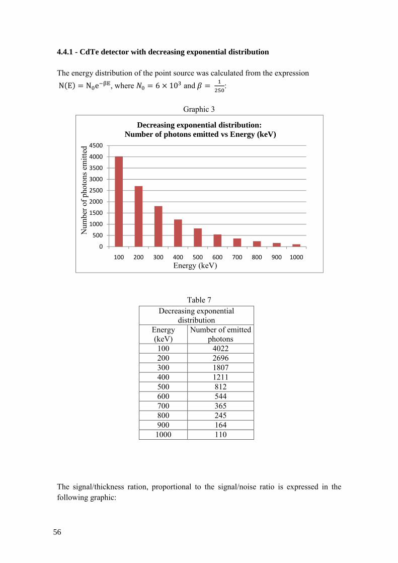
4.4.1 - CdTe detector with decreasing exponential distribution The energy distribution of the point source was calculated from the expression N"E# NJeGj, where kJ 6 m 10p and q H
'LJ:
Graphic 3
Table 7 Decreasing exponential
distribution Energy (keV)
Number of emitted photons
100 4022 200 2696 300 1807 400 1211 500 812 600 544 700 365 800 245 900 164
1000 110 The signal/thickness ration, proportional to the signal/noise ratio is expressed in the following graphic:
0
500
1000
1500
2000
2500
3000
3500
4000
4500
100 200 300 400 500 600 700 800 900 1000
Decreasing exponential distribution:Number of photons emitted vs Energy (keV)
Num
ber o
f pho
tons
emitt
ed
Energy (keV)
56

Graphic 8
Table 9 Thickness
(cm) Signal σS Signal/Thickness
(cm-1) σS/T
(cm-1) 12.55 11647 108 928 9 11.5 11641 108 1012 9
10.75 11637 108 1083 10 9.4 11585 108 1232 11 8.3 11529 107 1389 13
6.91 11400 107 1650 15 5.37 11164 106 2079 20 3.46 10496 102 3034 30 1.54 8793 94 5710 61
0.256 4821 69 18832 271 The thickness values considered were obtained by adjusting it so the detector would absorb ~90% of the photons emitted for a specific energy. For example, for a 100keV monoenergetic beam, a detector with a depth of 0.256 cm absorbs ~90% of the photons emitted. The signal represents the photons that left all their energy in the detector. This process obeys a Poissonian statistics and so, the error in the signal is considered to be the square root of the value. These results allow the conclusion that there is no preferable depth, since there is no thickness value that maximizes the ratio signal/noise. Concerning the efficiency, the results are:
0
2000
4000
6000
8000
10000
12000
14000
16000
18000
20000
0 2 4 6 8 10 12 14
Sinal/Thickness (cm-1) vs Thickness (cm) Decreasing exponential energy distribution
Thickness (cm)
Sign
al/T
hick
ness
(cm
-1)
57

Graphic 10
Table 11
Thickness (cm) P.I. σP.I. P.T. σP.T. i. efficiency σi.eff.
12.55 11967 109 11647 108 0.97 0.01 11.5 11961 109 11641 108 0.97 0.01
10.75 11962 109 11637 108 0.97 0.01 9.4 11945 109 11585 108 0.97 0.01 8.3 11917 109 11529 107 0.97 0.01
6.91 11852 109 11400 107 0.96 0.01 5.37 11728 108 11164 106 0.95 0.01 3.46 11303 106 10496 102 0.93 0.01 1.54 9837 99 8793 94 0.89 0.01
0.256 5431 74 4821 69 0.89 0.02 As expected, the efficiency increases with thickness, but remains almost constant after a certain point around a thickness of 8cm. This means that increasing the volume in order to increase the efficiency is useless since this volume increase would not be translated into a gain in the signal/noise ration. In order words, the gain in efficiency would be due mainly to the increase in the noise. 4.4.2 - CdTe detector with increasing exponential distribution The point source emits according to the following distribution law, obtained from the expression N"E# NJej, where kJ 70 and q H
'LJ:
0%
20%
40%
60%
80%
100%
0 2 4 6 8 10 12 14
Efficiency (%) vs Thickness (cm)Decreasing exponential energy distribution
Thickness (cm)
Effic
ienc
y (%
)
58

Graphic 6
Table 12 Increasing exponential
distribution Energies
(keV) Number of
photons 100 104 200 156 300 232 400 347 500 517 600 772 700 1151 800 1717 900 2562
1000 3822
0
500
1000
1500
2000
2500
3000
3500
4000
4500
100 200 300 400 500 600 700 800 900 1000
Increasing exponential distribution:Number of photons emitted vs Energy (keV)
Num
ber o
f pho
tons
emitt
ed
Energy (keV)
59

The signal/thickness ratio is given by the next graphic whose data is presented on table 13:
Graphic 7
Table 13
Thickness (cm) Signal σS
Signal/Thickness (cm-1)
σS/T (cm-1)
12.55 10465 102 834 8 11.5 10341 102 899 9
10.75 10234 101 952 9 9.4 9958 100 1059 11 8.3 9625 98 1160 12
6.91 8906 94 1289 14 5.37 7898 89 1471 17 3.46 5895 77 1704 22 1.54 2723 52 1768 34
0.256 361 19 1410 74 The result here obtained concerning the signal/noise ratio is interesting since there is a depth around 2cm that maximizes the signal/noise ratio. The next step is to investigate the efficiency, whose results are presented in the following graphic:
0
200
400
600
800
1000
1200
1400
1600
1800
2000
0 2 4 6 8 10 12 14
Sinal/Thickness (cm-1) vs Thickness (cm) Increasing exponential energy distribution
Thickness (cm)
Sign
al/T
hick
ness
(cm
-1)
60

Graphic 8
Table 14
These results show that between 0cm and 2cm, the increase in efficiency is mainly due to the increase in the signal. It is possible to conclude that increasing the depth over 2cm will not increase the detector’s performance. 4.4.3 - CdTe detector with uniform distribution In this case, I considered a source whose energy distribution is uniform between 100keV and 1000keV. The signal/thickness ratio is given by the following graphic:
0%
10%
20%
30%
40%
50%
60%
70%
80%
90%
100%
0 2 4 6 8 10 12 14
Efficiency (%) vs Thickness (cm)Increasing exponential energy distribution
Thickness (cm)
Effic
ienc
y (%
)
Thickness (cm) P.I. σP.I. P.T. σP.T. i. efficiency σi.eff.
12.55 11280 106 10465 102 0.93 0.01 11.5 11227 106 10341 102 0.92 0.01
10.75 11207 106 10234 101 0.91 0.01 9.4 11077 105 9958 100 0.90 0.01 8.3 10934 105 9625 98 0.88 0.01
6.91 10601 103 8906 94 0.84 0.01 5.37 10041 100 7898 89 0.79 0.01 3.46 8562 93 5895 77 0.69 0.01 1.54 5460 74 2723 52 0.50 0.01
0.256 1275 36 361 19 0.28 0.02
61

Graphic 9
Table 15 Thickness
(cm) Signal σS Signal/Thickness
(cm-1) σS/T
(cm-1) 12.55 9485 97 756 8 11.5 9408 97 818 8
10.75 9357 97 870 9 9.4 9238 96 983 10 8.3 9016 95 1086 11
6.91 8782 94 1271 14 5.37 8143 90 1516 17 3.46 6943 83 2007 24 1.54 4446 67 2887 43
0.256 1506 39 5883 152 Concerning the efficiency, the results obtained are given in graphic 10 and the corresponding data in presented in table 16:
0
1000
2000
3000
4000
5000
6000
7000
0 2 4 6 8 10 12 14
Sinal/Thickness (cm-1) vs Thickness (cm) Uniform energy distribution
Thickness (cm)
Sign
al/T
hick
ness
(cm
-1)
62

Graphic 10
Table 16 Thickness
(cm) P.I. σP.I. P.T. σP.T. i. efficiency σi.eff.
12.55 9964 100 9485 97 0.95 0.01 11.5 9947 100 9408 97 0.95 0.01
10.75 9927 100 9357 97 0.94 0.01 9.4 9864 99 9238 96 0.94 0.01 8.3 9778 99 9016 95 0.92 0.01
6.91 9653 98 8782 94 0.91 0.01 5.37 9372 97 8143 90 0.87 0.01 3.46 8486 92 6943 83 0.82 0.01 1.54 6195 79 4446 67 0.72 0.01
0.256 2247 47 1506 39 0.67 0.02
Once again, the results show that an improvement in the detector’s efficiency will not improve its performance, i. e., its signal/noise ratio. 4.4.4 - Si detector with uniform distribution Silicon is a material that may be used in the GRI mission’s payload for low energies. Thus, it is important to test this material. In this subsection I will do the same thing as I did in the previous one, except that this time, the material considered is different (silicon) and the thickness values considered
0%
20%
40%
60%
80%
100%
0 2 4 6 8 10 12 14
Efficiency (%) vs Thickness (cm)Uniform energy distribution
Thickness (cm)
Effic
ienc
y (%
)
63
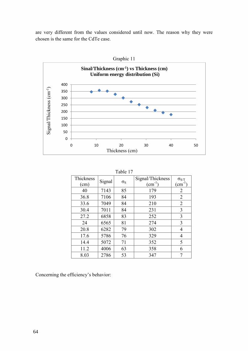
are very different from the values considered until now. The reason why they were chosen is the same for the CdTe case.
Graphic 11
Table 17
Thickness (cm) Signal σS
Signal/Thickness (cm-1)
σS/T (cm-1)
40 7143 85 179 2 36.8 7106 84 193 2 33.6 7049 84 210 2 30.4 7011 84 231 3 27.2 6858 83 252 3 24 6565 81 274 3
20.8 6282 79 302 4 17.6 5786 76 329 4 14.4 5072 71 352 5 11.2 4006 63 358 6 8.03 2786 53 347 7
Concerning the efficiency’s behavior:
0
50
100
150
200
250
300
350
400
0 10 20 30 40 50
Sinal/Thickness (cm-1) vs Thickness (cm) Uniform energy distribution (Si)
Thickness (cm)
Sign
al/T
hick
ness
(cm
-1)
64
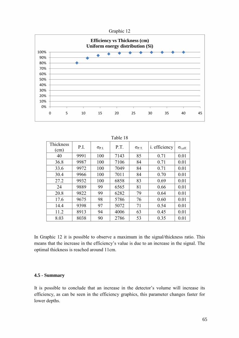
Graphic 12
Table 18
Thickness (cm) P.I. σP.I. P.T. σP.T. i. efficiency σi.eff.
40 9991 100 7143 85 0.71 0.01 36.8 9987 100 7106 84 0.71 0.01 33.6 9972 100 7049 84 0.71 0.01 30.4 9966 100 7011 84 0.70 0.01 27.2 9932 100 6858 83 0.69 0.01 24 9889 99 6565 81 0.66 0.01
20.8 9822 99 6282 79 0.64 0.01 17.6 9675 98 5786 76 0.60 0.01 14.4 9398 97 5072 71 0.54 0.01 11.2 8913 94 4006 63 0.45 0.01 8.03 8038 90 2786 53 0.35 0.01
In Graphic 12 it is possible to observe a maximum in the signal/thickness ratio. This means that the increase in the efficiency’s value is due to an increase in the signal. The optimal thickness is reached around 11cm. 4.5 - Summary It is possible to conclude that an increase in the detector’s volume will increase its efficiency, as can be seen in the efficiency graphics, this parameter changes faster for lower depths.
0%
10%
20%
30%
40%
50%
60%
70%
80%
90%
100%
0 5 10 15 20 25 30 35 40 45
Efficiency vs Thickness (cm)Uniform energy distribution (Si)
65
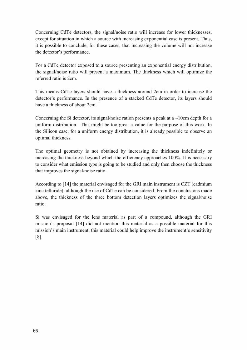
Concerning CdTe detectors, the signal/noise ratio will increase for lower thicknesses, except for situation in which a source with increasing exponential case is present. Thus, it is possible to conclude, for these cases, that increasing the volume will not increase the detector’s performance. For a CdTe detector exposed to a source presenting an exponential energy distribution, the signal/noise ratio will present a maximum. The thickness which will optimize the referred ratio is 2cm. This means CdTe layers should have a thickness around 2cm in order to increase the detector’s performance. In the presence of a stacked CdTe detector, its layers should have a thickness of about 2cm. Concerning the Si detector, its signal/noise ration presents a peak at a ~10cm depth for a uniform distribution. This might be too great a value for the purpose of this work. In the Silicon case, for a uniform energy distribution, it is already possible to observe an optimal thickness. The optimal geometry is not obtained by increasing the thickness indefinitely or increasing the thickness beyond which the efficiency approaches 100%. It is necessary to consider what emission type is going to be studied and only then choose the thickness that improves the signal/noise ratio. According to [14] the material envisaged for the GRI main instrument is CZT (cadmium zinc telluride), although the use of CdTe can be considered. From the conclusions made above, the thickness of the three bottom detection layers optimizes the signal/noise ratio. Si was envisaged for the lens material as part of a compound, although the GRI mission’s proposal [14] did not mention this material as a possible material for this mission’s main instrument, this material could help improve the instrument’s sensitivity [8].
66

References for Chapter 4 [1] - Leo, W. R., "Techniques for Nuclear and Particle Physics Experiments"(2nd revised edition), Springer-Verlag, 1994 [2] - Knoll, G., “Radiation Detector and Measurement” (3rd edition), John Wiley & Sons, 2000 [3] - Pisa, A.,"Hard X–ray Optics Development: Feasibility Study of a Laue Lens", PhD Thesis, 2004 [4] - Takahashi, T., “A Si/CdTe Compton Camera for gamma-ray lens experiment”, Exp. Astro., vol. 20, 317-331 (2006) [5] - Frontera, F. et al., “Exploring the hard x-/soft gamma-ray continuum spectra with Laue lenses”, 39TH ESLAB Symposium on Trends in Space Science and Cosmic Vision 2020, 2005 [6] - Agostinelli, S., et al., “Geant4 – a simulation toolkit”, N.I.M. A, vol. 506, 250-303 (2003) [7] - Caroli, E., et al., “Polarisation measurements with a CdTe pixel array detector for Laue hard X-ray focusing telescopes”, Exp. Astron., vol. 20, 353–364 (2005) [8] - Zoglauer, A., et al., “Simulated Performance of CZT-Based Focal Plane Detectors for Gamma-Ray Lenses”,2006 IEEE Nuclear Science Symposium Conference Record (2006) [9] - Weisskopf, M. C., et al.,“On understanding the figures of merit for detection and measurement of x-ray polarization” (arXiv:1006.3711v2) [10] - P.I. Jürgen Knödlseder, “GRI exploring the extremes”, submitted proposal to Cosmic Vision 2015-2025 call for missions, June 2007 [11] - Curado da Silva, R. M., et al., “Cipher: a polarimeter telescope concept for hard x-ray astronomy”, Exp. Astron., vol. 15, 45-65 (2003) [12] - Kroeger, R. A., et al., “Gamma ray instrument for polarimetry, spectroscopy and imaging (GIPSI), SPIE proceedings on Gamma-Ray and Cosmic-Ray Detectors, Techniques, and Missions, vol. 2806, 52-63 (1996)
67

[13] - Stephen, J. B., et al., “Gamma-ray polarization and measurements with INTEGRAL/IBIS”, AIP Conference Proceedings series, presented in Gamma-Ray Astrophysics 2001, Baltimore, Maryland, U.S.A. [14] - P.I. Jürgen Knödlseder, “GRI exploring the extremes”, submitted proposal to Cosmic Vision 2015-2025 call for missions, June 2007 [15] - Lei, F., Dean, A.J., and Hills, G.L., “Compton Polarimetry in Gamma-Ray Astronomy”, Space Science Reviews, vol. 82, 309-388 (1997) [16] - Pearson, W. B., “A handbook of Lattice and Structures of Metals and Alloys”, Pergamon Press, reprinted with corrections (1964)
68

Chapter 5
Instrument sensitivity: Comparison between two solutions
69

In this chapter, one of the major results of this work is presented. Sensitivity is a parameter that must be considered when improving an instrument’s performance. Laue lens are a technical development that will accomplish this purpose. However, another approach can be considered. A stacked detector is presented in [1] and, according to this reference, it is possible to increase sensitivity by dividing the detection’s volume in several layers. Thus, it is important to confront the two approaches in order to verify which one could have more impact in improving sensitivity, since, in terms of technical complexity and cost, both solutions have different implications when setting up a gamma-ray mission. 5.1 - Introduction The simulations presented in this chapter were made in order to verify the hypothesis presented in [1], since its basis have never been duly presented in works. This hypothesis states that a stacked detector will present a better sensitivity than a monolithic one. This is acceptable, since it is easier to trace a photon’s path inside a stacked detector than in a monolithic one. I will consider three different geometries, all made of squared surface layers with equal area. However, their thicknesses change with the number of layers, since the detector’s volume is the same for all the geometries used. The geometries tested are based on [1]. In fact, one of these geometries (geometry 3) presents almost the same characteristics as the geometry present in [1], except that, in this work, a ceramic sheet between layers was not simulated. The separation between layers is 0.7mm for all cases. The next table and figures present the characteristics of each geometry considered.
Table 1
Geometry
Number of
layers
Layers’
dimensions (mm3)
Pixels
dimensions (mm3)
Distance
between Pixels (mm)
Distance between last pixel and the layer’s
border (mm)
1
4
21.5 x 21.5 x 5
2.0x2.0x5.0
0.15
0.075
2
20
21.5 x 21.5 x 1.0
2.0x2.0x1.0
0.15
0.075
3
40
21.5 x 21.5 x 0.5
2.0x2.0x0.5
0.15
0.075
70

For all the geometries considered, the material volume is the same: 9.245cm3. The figures below present information that helps to visualize the geometries in question.
Fig. 1: This figure represents each layer’s surface, which is the same for all the geometries considered. The yellow squares represent the pixels and the brown areas represent the separations between pixels and between a pixel and the detector’s border. All the dimensions are presented in the amplified circle.
Fig. 3: The brown line represents the position at which the source is centered: (0,0, 5cm). The dotted line marks the height attained by the detector’s surface: 1.105cm (geometry 1), 1.665cm (geometry 2) or 2.365cm (geometry 3). Thus, the distance between the source and the detector’s surface can be 3.895cm (geometry 1), 3.335cm (geometry 2) or 2.635cm (geometry 3). The distances mentioned are independent of the source used.
Fig. 2: This figure represents two adjacent layers. Their separation is 0.7mm for all cases. However, the value represented by the letter “d” can be 5mm (geometry 1), 1mm (geometry 2) or 0.5mm (geometry 3).
71

As was seen in Chapter 4, the sensitivity’s expression is:
F
(5.1)
βs+a and βs are the events reconstructed from simulations performed with a photons’ source with and without the material’s activation respectively. The source’s observation time was the same for all the simulations performed and it is possible to evaluate the counts corresponding to background noise. By knowing the time during which these counts were observed ∆t and the detector’s sensitive area A, it is possible to write: B
∆ (5.2)
η ~ β β (5.3) With the MEGAlib package [3] it is possible to know the values of βs+a and βs. Thus, using eq. 5.2 it is possible to calculate B, since all the other variables are known. The exact relationship between the variable η and the total number of background events (β β) will be explained in section 5.4. With the Geant4 toolkit [1] it is possible to obtain the efficiency’s value. By using eq. 5.1 and the value of B previously calculated, it is possible to calculate the sensitivity. This was the task performed and described in this chapter. 5.2 - The MEGAlib and event reconstruction An event can be considered as the particle’s history, from the time it is created until it is absorbed or leaves the detector. As stated in [4], an event is a collection of hits and each hit is characterized by the coordinates of the position where an interaction took place and a value for the energy deposited. Organizing these hits in the correct order by making use or statistics and physical laws is the event reconstruction’s aim. In the considered energy range, a photon can interact with matter by three possible ways: photoelectric absorption, pair production and Compton interaction. According to [4], events that correspond to pair production leave a distinctive mark in a tracker: an inverted “V” shape. Generally, a hit corresponding to an interaction can be found in one layer and two hits appear in the next layers. A Compton interaction is more complicated to analyze, since there might be a large number of hits that must be organized. If there are n hits, there will be n! ways to organize them. It is worth noting that, due computational limitations, an event can be
72

excluded from reconstruction if it is the result of too many hits. In the simulations performed, n was limited to 5. In order to choose what is the most likely option among the n! possible ways, it is necessary to appeal to statistical tools. In statistics, the correlation coefficient indicates the strength of the linear dependence between two variables. [5]. If X and Y are two probabilistic variables, this coefficient can be written as: covX, Y X · Y%%%%%% X& · Y& (5.4) If this coefficient equals 0, the two variables are independent, if it equals 1 they vary in the same sense: if X increases, Y will also increase. If it equals -1, the variables will vary in opposite senses: X decreases while Y increases. The event reconstruction, in this work, was performed using the Pearson correlation coefficient (cP), which means that the correlation coefficients used have the following expression:
c'X, Y ()*+,,-.-/ (5.5)
Where σ+ and σ, are the variances of X and Y respectively. The variables considered for reconstruction are the energy deposited by the particle (Edep), the change in the electron’s direction along the track (∆α) and “i”, the hit ID along it. The Pearson correlation coefficient is considered for a two pairs of probabilistic variables: (Edep, i) and (∆α, i). For the correct sequence, positive correlation coefficients for both pairs are expected [4]:
c'12)3E516,i8 9:;·<%%%%%%%%%= 9:;%%%%%%%·<>9:;?%%%%%%%=9:;%%%%%%%?@<?& =<>?
(5.6)
c'12)Δα, i CD·<%%%%%%= CD%%%%%·<>@CD?%%%%%%=CD%%%%?@<?& =<>? (5.7)
For each Compton event a quality factor can be defined as:
Q9,'12) 1 (G:HIJK39:;,8(G:HIJK∆D,L (5.8)
The lower the quality factor is, the better the track obtained agrees with the physics considered. In this study only events with a Q factor between 0 and 0.05 were accepted. MEGAlib (Medium Energy Gamma-ray Astronomy library) [4] is a software toolkit that allows the simulation of a detector’s response and the data analysis, including event reconstruction. Cosima (Cosmic Simulator for MEGAlib) is part of MEGAlib [4] and it is the software that was used to simulate the detector’s response to the sources
73

considered. Revan (Real event analyzer) [6] was the program used to perform event reconstruction and is also part of MEGAlib [4]. 5.3 - The simulations It is quite important to state which assumptions were made for the simulations. Due to time and CPU constraints, simulations performed with Geant4 did not take into account pixels. However, those were simulated when using MEGAlib [4], since pixels would have a much greater impact in the events’ reconstruction than in efficiency. Considering a stacked detector, dividing a layer into several sensitive volumes (pixels) is expected to increase the number of events reconstructed, since the volume within which the interaction was registered is smaller for a pixel than for the entire layer’s volume. Thus, the interaction’s position can be determined more accurately, making the event’s reconstruction more efficient. The geometries considered were exposed to two kinds of sources: a source that covered only a circle with a 2mm radius (point source) and a source that covered the entire detector’s surface. For each geometry and source, the value of βs+a was obtained by simulating the exposure of the detector to photons from the source and from the material’s activation. The value of βs was obtained by exposing the detector to the source only. The next table presents characteristics common to all three geometries considered for simulation. They are part of the input parameters used by Cosima [4]. The values considered for energy resolution were taken from [1].
Table 2 Noise threshold (keV) 10keV
Signal Threshold (keV) 10keV Energy resolution at 1.17 MeV (FWHM) 1.6% Energy resolution at 1.33MeV (FWHM) 1.7%
Photons Flux (particles/s) 10 Proton Flux (particles/s) 3.73
Irradiation time for photons (s) 5000 Irradiation time for protons (s) 3.1556736 x 10⁷ (~1year)
The two first entries state that no energy depositions under 10keV (typical setup value) were considered for event reconstruction in order to minimize CdTe noise. The values for energy resolution were based on [1]. The protons’ flux (responsible for the material’s activation) and the irradiation time for protons are typical values for gamma-ray astronomy. Simulations with and without activation were performed and, for the second case, the Proton Flux and the Irradiation time for protons were not considered.
74

In section 5.4, the background flux is calculated by making use of the MEGAlib [4] toolkit. In section 5.5 the results obtained with Geant4 for efficiency are presented. In section 5.6 the results of the previous sections are combined in order to perform the sensitivity’s calculation. In section 5.7 the conclusions of this chapter are presented. 5.4 - The background flux The background flux was calculated by making use of equation 5.2. The value of βs+a corresponds to the events reconstructed in a situation where the detector is irradiated with photons from the source and activation and the value of βs corresponds to the events reconstructed when the detector is exposed only to photons from the source. βs+a- βs corresponds to the reconstructed background noise events. Due to time constraints, the only background flux considered is due to the material’s activation, but, from a qualitative point of view, considering other background sources would change the results by a scale factor only. The first step is to obtain the value of βs+a - βs. However, this value needs to be corrected since, as it is possible to trace events that are due to background, and, because the source’s position is known, only those background events crossing the first layer cannot be clearly separated from the events due to the source only. Thus, the value of βs+a - βs was multiplied by the solid angle subtended by the detector’s surface exposed to the source divided by 4M. The variable η was this value multiplied by a factor of two since it is not possible to distinguish a background event entering the detector or coming out of it. The solid angle was calculated by integration the expression: NΩ sin RNRNS (5.9) In which the angle θ varies from zero to the angle formed by the vertical axis and the line between the detector’s corner and its center. The angle φ varies from zero to 2M. In fact, since the detectors’ surface is a square, the limiting angle θ will depend on φ, but the approximation considered is reasonable. The value of η was used to calculate the background flux. Tables 3 and 4 present the calculation of η and tables 5 and 6 present the background flux obtained.
Table 3 Plane source
4 layers
E(keV) βs+a σ(βs+a) βs σ(βs) βs+a - βs σ(βs+a - βs) TΩ4MV η σ(η)
100 89031 597 40384 402 48647 720 0.2060 20045 296
75

400 25921 322 12491 224 13430 392 5534 162 700 8948 189 3912 125 5036 227 2075 93
1000 4831 139 1880 87 2951 164 1216 68 20 layers
100 84664 1301 39791 892 44873 1577
0.1308
11736 413 400 25509 714 11296 475 14213 858 3717 224 700 8040 401 3424 262 4616 479 1207 125
1000 4126 287 1464 171 2662 334 696 87 40 layers
100 84566 1839 38995 1249 45571 2223
0.0794
7237 353 400 21559 929 10137 637 11422 1126 1814 179 700 7112 533 2792 334 4320 629 686 100
1000 3571 378 1163 216 2408 435 382 69
Table 4 Point source
4 layers
E(keV) βs+a σ(βs+a) βs σ(βs) βs+a - βs σ(βs+a - βs) TΩ4MV η σ(η)
100 86507 588 41793 409 44714 716
0.2060
18425 295 400 23400 306 10265 203 13135 367 5412 151 700 6418 160 3100 111 3318 195 1367 80
1000 3232 114 1249 71 1983 134 817 55 20 layers
100 86613 1316 41039 906 45574 1598
0.1308
11919 418 400 19312 621 8431 411 10881 745 2846 195 700 5127 320 2268 213 2859 384 748 101
1000 2364 217 814 128 1550 252 405 66 40 layers
100 76865 1753 38425 1240 38440 2147
0.0794
6105 341 400 16621 815 7062 531 9559 973 1518 155 700 3774 389 1675 259 2099 467 333 74
1000 1565 250 475 138 1090 286 173 45 The columns marked with the symbol σ represent the estimated error for the variable presented in the previous column. The errors of the variables marked with β were calculated by dividing the number of reconstructed events by the number of layers, thus obtaining the average number of events in one layer. Taking the square root would give the estimated error for one layer, so this number was again multiplied by the number of layers. By applying the propagation error formulae, it is possible to calculate the error in βs+a - βs:
Table 3 (cont.)
76

σβ β @σβs W a W σβs (5.10) The propagation error formula states that, if f(x,y,z,..) is a function of the measured variables x, y, z, … Then, the error in the function f depends on the error of each measured variable according to eq. 5.10:
∆f Z[\[]^ ∆x W Z[\
[`^ ∆y W Z[\[b^ ∆z W d (5.11)
No error were considered in the variables ∆t, As, ∆E, which means that the error of B was calculated by dividing the values in the column marked as σ(βs+a - βs) by the three variables already mentioned. The next tables present the background noise flux calculated from η. The observation time ∆t corresponds to the time during which the background was observed: 3.1556736 x 10⁷ (~1year). The results obtained are presented for both sources in the following tables (the units of B and σB are 10-6cm-2s-1):
Table 5 Plane source
4 layers E
(keV) η σ(η) ∆t (s) B σ(B)
100 20045 296
31556736
13.2 0.2 400 5534 162 3.7 0.1 700 2075 93 1.37 0.06
1000 1216 68 0.80 0.04 20 layers
100 11736 413
31556736
2.11 0.07 400 3717 224 0.67 0.04 700 1207 125 0.22 0.02
1000 696 87 0.13 0.02 40 layers
100 7237 353
31556736
0.68 0.03 400 1814 179 0.17 0.02 700 686 100 0.065 0.009
1000 382 69 0.036 0.007
77

Table 6 Point Source
4 layers E
(keV) η σ(η) ∆t (s) B σ(B)
100 18425 295
31556736
12.2 0.2 400 5412 151 3.6 0.1 700 1367 80 0.90 0.05
1000 817 55 0.54 0.04 20 layers
100 11919 418
31556736
2.15 0.08 400 2846 195 0.51 0.04 700 748 101 0.13 0.02
1000 405 66 0.07 0.01 40 layers
100 6105 341
31556736
0.58 0.03 400 1518 155 0.14 0.01 700 333 74 0.03 0.01
1000 173 45 0.016 0.004 The value of B for all cases is present in the following graphic:
Graphic 1
The value of the background noise flux needed for the sensitivity’s calculation was obtained and it is possible to see that it decreases with energy and with the number of
0
2
4
6
8
10
12
14
0 500 1000 1500
4 layers - Plane source
20 layers - Plane source
40 layers - Plane source
4 layers - Point source
20 layers - Point source
40 layers - Point source
Energy (keV)
Bac
kgro
und
nois
e flu
x (1
0-6cm
-2s-1
)
Background noise flux (10-6cm-2s-1) vs Energy (keV)
78

layers. The next table presents the percentage of reconstructed events due to background noise (activation) in the total reconstructed events.
Table 7
Planar source Point source 4 layers
E (keV) βs+a βs (βs+a - βs)/ βs+a (%) βs+a βs (βs+a - βs)/ βs+a (%) 100 89031 40384 54.64 86507 41793 51.69 400 25921 12491 51.81 23400 10265 56.13 700 8948 3912 56.28 6418 3100 51.70
1000 4831 1880 61.08 3232 1249 61.36 20 layers
100 84664 39791 53.00 86613 41039 52.62 400 25509 11296 55.72 19312 8431 56.34 700 8040 3424 57.41 5127 2268 55.76
1000 4126 1464 64.52 2364 814 65.57 40 layers
100 84566 38995 53.89 76865 38425 50.01 400 21559 10137 52.98 16621 7062 57.51 700 7112 2792 60.74 3774 1675 55.62
1000 3571 1163 67.43 1565 475 69.65
Generally, the number of background noise (activation) reconstructed events increases with the number of layers. Thus it is possible to know the trajectories of more events due to activation and subtract them to the signal (source+activation) obtained. This will contribute to improve sensitivity since more events from background noise can be traced and eliminated. 5.5 - Efficiency The next tables present the results and calculations obtained for efficiency. P.I. stands for Photons that Interacted, which means photons that left part or all of their energy within the detector, P.T stands for Photons that left their Total energy within the detector. The symbol ed corresponds to the efficiency value present in eq. 5.1 and the estimated errors for this variable are given in the column signaled by σ(ed).
Table 8 Plane source
4 layers E (keV) P. I. σP.I. P. E. σP.E. ed σ(ed)
100 100000 632 99217 630 0.992 0.009 400 72893 540 43976 419 0.603 0.007 700 57779 481 20895 289 0.362 0.006
1000 50068 448 13251 230 0.265 0.005
79
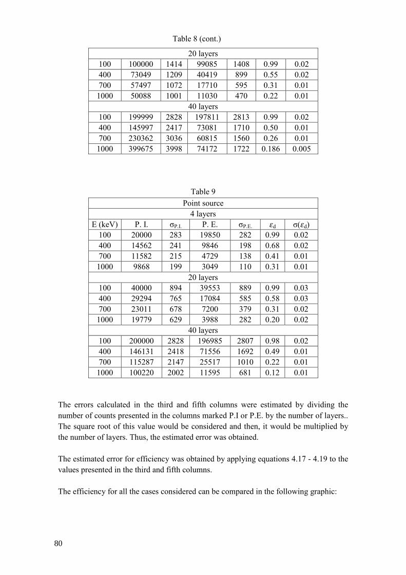
20 layers 100 100000 1414 99085 1408 0.99 0.02 400 73049 1209 40419 899 0.55 0.02 700 57497 1072 17710 595 0.31 0.01
1000 50088 1001 11030 470 0.22 0.01 40 layers
100 199999 2828 197811 2813 0.99 0.02 400 145997 2417 73081 1710 0.50 0.01 700 230362 3036 60815 1560 0.26 0.01
1000 399675 3998 74172 1722 0.186 0.005
Table 9 Point source
4 layers E (keV) P. I. σP.I. P. E. σP.E. ed σ(ed)
100 20000 283 19850 282 0.99 0.02 400 14562 241 9846 198 0.68 0.02 700 11582 215 4729 138 0.41 0.01
1000 9868 199 3049 110 0.31 0.01 20 layers
100 40000 894 39553 889 0.99 0.03 400 29294 765 17084 585 0.58 0.03 700 23011 678 7200 379 0.31 0.02
1000 19779 629 3988 282 0.20 0.02 40 layers
100 200000 2828 196985 2807 0.98 0.02 400 146131 2418 71556 1692 0.49 0.01 700 115287 2147 25517 1010 0.22 0.01
1000 100220 2002 11595 681 0.12 0.01 The errors calculated in the third and fifth columns were estimated by dividing the number of counts presented in the columns marked P.I or P.E. by the number of layers.. The square root of this value would be considered and then, it would be multiplied by the number of layers. Thus, the estimated error was obtained. The estimated error for efficiency was obtained by applying equations 4.17 - 4.19 to the values presented in the third and fifth columns. The efficiency for all the cases considered can be compared in the following graphic:
Table 8 (cont.)
80

Graphic 2
The efficiency decreases with the number of layers. This behavior is expected since the detector with 4 layers is the closest to a monolithic detector. 5.6 - Sensitivity With the background noise values obtained in section 5.4, the efficiency values obtained in section 5.5 and using eq. 5.1, the sensitivity (F) was calculated. The following tables contain all the data used to perform this calculation (the units of B and σB are 10-6cm-2s-1 and the units of F and σF are 10-5cm-2s-1):
Table 10 Plane source
4 layers E (keV) ed σ(ed) B σB S t (s) Ad (cm2) F σF
100 0.992 0.009 13.2 0.2
3 5000 4
11.0 0.2 400 0.603 0.007 3.7 0.1 9.5 0.3 700 0.362 0.006 1.37 0.06 9.7 0.5
1000 0.265 0.005 0.80 0.04 10.1 0.6 20 layers
100 0.99 0.02 2.11 0.07
3 5000 4
4.4 0.2 400 0.55 0.02 0.67 0.04 4.5 0.3 700 0.31 0.01 0.22 0.02 4.5 0.5
1000 0.22 0.01 0.13 0.02 4.8 0.6
0%
10%
20%
30%
40%
50%
60%
70%
80%
90%
100%
0 500 1000 1500
4 layers - Plane source
20 layers - Plane source
40 layers - Plane source
4 layers - Point source
20 layers - Point source
40 layers - Point source
Energy (keV)
Effic
ienc
y
Efficiency (%) vs Energy (keV)
81

40 layers 100 0.99 0.02 0.68 0.03
3 5000 4
2.5 0.1 400 0.50 0.01 0.17 0.02 2.5 0.2 700 0.26 0.01 0.065 0.009 2.9 0.4
1000 0.186 0.005 0.036 0.007 3.1 0.6
Table 11
Point source 4 layers
E (keV) ed σ(ed) B σB S t (s) Ad (cm2) F σF 100 0.99 0.02 12.2 0.2
3 5000 4
10.6 0.3 400 0.68 0.02 3.6 0.1 8.3 0.3 700 0.41 0.01 0.90 0.05 7.0 0.4
1000 0.31 0.01 0.54 0.04 7.1 0.5 20 layers
100 0.99 0.03 2.15 0.08
3 5000 4
4.4 0.2 400 0.58 0.03 0.51 0.04 3.7 0.3 700 0.31 0.02 0.13 0.02 3.6 0.5
1000 0.20 0.02 0.07 0.01 4.1 0.8 40 layers
100 0.98 0.02 0.58 0.03
3 5000 4
2.3 0.1 400 0.49 0.01 0.14 0.01 2.3 0.2 700 0.22 0.01 0.03 0.01 2.4 0.5
1000 0.12 0.01 0.016 0.004 3.2 0.9 The following graphic presents a comparison between sensitivity for all cases:
Graphic 3
0
2
4
6
8
10
12
0 500 1000 1500
4 layers - Plane source
20 layers - Plane source
40 layers - Plane source
4 layers - Point source
20 layers - Point source
40 layers - Point source
Energy (keV)
Sens
itivi
ty (1
0-5cm
-2s-1
)
Sensitivity (10-5cm-2s-1) vs Energy
Energy (keV)
Table 10 (cont.)
82

Generally, sensitivity improves with the number of layers since its value decreases. 5.7 - Conclusion The next tables present the number of times sensitivity is improved by passing from 4 to 20 layers and from 20 to 40 layers.
Table 12 Plane source
Increase in the number of layers 100keV 400keV 700keV 1000keV 4->20 2.50 2.13 2.15 2.10
20->40 1.76 1.80 1.54 1.58
Table 13 Point source
Increase in the number of layers 100keV 400keV 700keV 1000keV 4->20 2.38 2.25 1.96 1.75
20->40 1.91 1.60 1.47 1.27 Tables 12 and 13 indicate that increasing the number of layers from 4 to 20 has a greater impact in the sensitivity gain than increasing the number of layers from 20 to 40. The increase in the number of layers has more impact in the case of a plane source, especially for higher energies. The INTEGRAL mission is an example of a mission that was used to give an overview of the sky. However, it is also important a mission that observes specific objects so that non-thermal processes can be studied and the questions that originated the Cosmic Vision program (Chapter 1) can be answered. This can only be achieved by improving the sensitivity. As the GRI mission’s purpose is to study specific process and not map the sky, it is important to ensure that the GRI’s main instrument has the highest possible sensitivity. According to [7] a Laue mission can achieve a sensitivity of 10-6 cm-2s-1 at 511keV. Comparing this value with the sensitivity given for the SPI instrument on INTEGRAL: 2.8 x 10⁻⁵ cm-2s-1 at 511keV [11], it is seen that a Laue lens allows an improvement of 28 times in the sensitivity’s value. Dividing the detection volume doesn’t seem to have that impact, since sensitivity would increase by a value between ~1.27 to ~2.50 times. By combining the two solutions, an increase of sensitivity between ~35.56 and ~70 times would be expected. Nowadays, both solutions have already been tested. The results presented in section 5.6 for sensitivity have the same order of magnitude than the SPI’s sensitivity, indicating that dividing the volume in layers has much less impact on the sensitivity values than the use of Laue lens.
83

The CLAIRE project [8] was an experiment in which the performance of a Laue lens during a balloon flight was tested. The lenses consisted of 556 germanium-silicon crystals mounted on a titanium frame with a diameter of 45cm. The lens focused 170keV into a focal spot at a distance of 277cm. This was a major step to prove the Laue lens’ feasibility According to [9] the lens payload could cost from 20 to 30 million Euros. The benefit would be an improvement in sensitivity of 28 times over INTEGRAL’s sensitivity. Dividing the detection volume in several layers would not be so expensive, in comparison; however, only a small gain in sensitivity would be obtained, since 2.5 is much lower than 28. A Laue lens is more difficult to implement since, according to [10], the planes of every single mosaic crystal must be aligned according to a very specific angle. As for the stacking solution, it is important to ensure that there are no inactive regions at the bottom of each layer, so the charges generated within the layer can be completely collected [1]. Concerning the field of view, the stacked detector considered in [1] had a copper collimator that restricted it to 30’ for energies lower than 100keV. An opening angle of 4 degrees at 500keV is possible due to a BGO shield. As for the lens tested in the CLAIRE, the field of view is 90’’ [8] and, according to [9] it will be 5’ for the GRI mission’s optics. For a mission designed to study specific objects it is quite important to have a narrow field of view, since an incident gamma-ray whose incident direction is not within it can be considered as background. Taking into account the values obtained for the field of view concerning different solutions, it is possible to verify that the Laue lenses have a lower field of view, making this solution more interesting as a way to increase sensitivity. As a final remark, it should be noted that the use of the MEGAlib software [4] is quite recent in this Physics Department. Thus, further studies are required to verify the accuracy of the results obtained with this software. Although it is possible that different values for βs+a and βs may be obtained, it is unlikely that this fact will change the conclusions obtained in this work.
84

References for Chapter 5 [1] - Takahashi, T., “A Si/CdTe Compton Camera for gamma-ray lens experiment”, Focusing Telescopes in Nuclear Astrophysics, Section III, 317-331 (2006) [2] - Agostinelli, S., et al., “Geant4 – a simulation toolkit”, N.I.M. A, vol. 506, 250-303 (2003) [3] - Zoglauer, A., Andritschke, R., Schopper, F, "MEGAlib - The Medium Energy Gamma-ray Astronomy Library", New Astronomy Reviews, Vol. 50, Issues 7-8, Pages 629-632 (2006) [4] - Zoglauer, A., "First Light for the Next Generation of Compton and Pair Telescopes", Doctoral thesis, TU Munich, 2005 [5] - Pestana, D.D., Velosa, S. F., "Introdução à Probabilidade e à Estatística", Fundação Calouste Gulbenkian, 2002 [6] - http://www.mpe.mpg.de/MEGA/software/MEGAlib.pdf [7] - Wunderer, C., “γ-Ray lenses – taking a deeper look at sites of nucleosynthesis”, New Astro. Rev., vol 50, 613–618 (2006) [8] - von Ballmoos, P., et al., “CLAIRE’s first light”, New Astron. Rev., 48, 243–249 (2004) [9] - P.I. Jürgen Knödlseder, “GRI exploring the extremes”, submitted proposal to Cosmic Vision 2015-2025 call for missions, June 2007 [10] - Pisa, A., e tal., “Feasibility study of a Laue lens for hard X–rays for space astronomy”, arXiv:astro-ph/0411574v2 [11] - http://sci.esa.int/science-e/www/object/index.cfm?fobjectid=31175&fbodylongid=719
85


Chapter 6
Polarimetry
87

This last chapter is to report some conclusions about polarization measurements obtained using a simplified version of the GRI main detector’s geometry. 6.1 - The Q factor According to [1], in a medium where the electrons’ density is 1cm-3, the probability that a polarized photon with energy E suffers a Compton interaction is given by dσ. If dΩ is the solid angle within which the scattered photon will appear with energy given by E’, then, the polarimetric differential cross-section is given by: Ω
2sinθcosφ (6.1)
The constant r is the classical electron radius. The angle θ is the angle between the incident direction and the scattering direction and the angle φ is the azimuthal scatter angle. It is possible to conceive a beam of a polarized photons impinging on one of the detectors considered in the previous chapter. The distance between pixels in these detectors is symmetrical in the XY directions. If a beam of 100% polarized photons impinges on a layer, and considering only photons that are scattered in a pixel and absorbed in another, their distribution will depend on . Fig.1: Scattering of a particle in a pixel.
88

The Q factor can be expressed as:
Q !"#º%& !"º% !"#º%' !"º% (6.2)
Rewritting this using eq. 6.1:
Q ()*+,, ' ,
,&()*+ (6.3)
Eq. 6.3 expresses the fact that, if the scattering angle is null, the Q factor will be zero and there will be no difference between the behavior of a polarized and a non-polarized particle. A polarimeter cannot measure a Q factor higher than the one given by eq. 6.3
for a specific values of the scattering angle and ε . However, due to geometrical
constraints, the Q value measured by a real polarimeter is always inferior to this number. The maximum Q values obtained for three angles are given in the following table:
Table 1 Scattering angle (θ) Maximum Q(.) value
0 0
/0 (45º)
8. 4. 1% 15
/ (90º)
4. 2. 1% 3
Thus, for an given incident angle, the higher the Q value measured, the better is the polarimeter, since its ability to identify a beam as polarized is greater. 6.2 - The Q factor for a specific geometry exposed to monoenergetic sources The Point Spread Function (PSF) is the reconstructed direction’s probability distribution of the gamma-rays that have their origin in a point source [2]. The detector considered in this chapter has one top layer 5mm thick and 3 bottom layers 20mm thick. All layers are separated by 20mm and divided in 64 x 64 pixels, each pixel having an area of 2.5x2.5mm2. This detector was irradiated with photons generated by a PSF corresponding to photons emitted by the Crab source passing through a Laue lenses. There were four different situations simulated corresponding to a low (LE) and high energy Laue lens (HE) combined with a source aligned with the detector’s axis or misaligned by 20’. The results for each layer are presented in the following table. Layer 1 corresponds to the top layer exposed to the source and layer 4 is the bottom one.
89
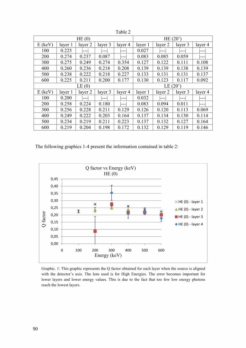
Table 2 HE (0) HE (20’)
E (keV) layer 1 layer 2 layer 3 layer 4 layer 1 layer 2 layer 3 layer 4 100 0.225 |---| |---| |---| 0.027 |---| |---| |---| 200 0.274 0.237 0.087 |---| 0.083 0.085 0.059 |---| 300 0.275 0.249 0.274 0.354 0.127 0.122 0.111 0.108 400 0.260 0.236 0.218 0.208 0.139 0.139 0.138 0.139 500 0.238 0.222 0.218 0.227 0.133 0.131 0.131 0.137 600 0.225 0.211 0.200 0.177 0.130 0.123 0.117 0.092
LE (0) LE (20’) E (keV) layer 1 layer 2 layer 3 layer 4 layer 1 layer 2 layer 3 layer 4
100 0.200 |---| |---| |---| 0.032 |---| |---| |---| 200 0.258 0.224 0.180 |---| 0.083 0.094 0.011 |---| 300 0.256 0.228 0.211 0.129 0.126 0.120 0.113 0.069 400 0.249 0.222 0.203 0.164 0.137 0.134 0.130 0.114 500 0.234 0.219 0.211 0.223 0.137 0.132 0.127 0.164 600 0.219 0.204 0.198 0.172 0.132 0.129 0.119 0.146
The following graphics 1-4 present the information contained in table 2:
0,00
0,05
0,10
0,15
0,20
0,25
0,30
0,35
0,40
0,45
0 100 200 300 400 500 600
HE (0) - layer 1
HE (0) - layer 2
HE (0) - layer 3
HE (0) - layer 4
Q factor vs Energy (keV)HE (0)
Q fa
ctor
Energy (keV)
Graphic. 1: This graphic represents the Q factor obtained for each layer when the source is aligned with the detector’s axis. The lens used is for High Energies. The error becomes important for lower layers and lower energy values. This is due to the fact that too few low energy photons reach the lowest layers.
90

Graphic. 2: This graphic represents the Q factor obtained for each layer when the source is aligned with the detector’s axis. The lens used is for Low Energies. The error becomes important for the reason pointed for the previous case.
Graphic. 3: This graphic represents the Q factor obtained for each layer when the source is 20’ off from the detector’s axis. The lens used is for High Energies. The error becomes important for the reason pointed for first case.
0
0,05
0,1
0,15
0,2
0,25
0,3
0 100 200 300 400 500 600
LE (0) layer 1
LE (0) layer 2
LE (0) layer 3
LE (0) layer 4Q fa
ctor
Energy (keV)
Q factor vs Energy (keV)LE (0)
-0,1
-0,05
0
0,05
0,1
0,15
0,2
0 100 200 300 400 500 600
HE (20') layer 1
HE (20') layer 2
HE (20') layer 3
HE (20') layer 4Q fa
ctor
Energy (keV)
Q factor vs Energy (keV)HE (20')
91
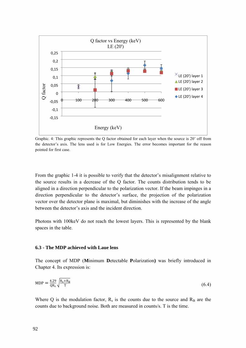
Graphic. 4: This graphic represents the Q factor obtained for each layer when the source is 20’ off from the detector’s axis. The lens used is for Low Energies. The error becomes important for the reason pointed for first case. From the graphic 1-4 it is possible to verify that the detector’s misalignment relative to the source results in a decrease of the Q factor. The counts distribution tends to be aligned in a direction perpendicular to the polarization vector. If the beam impinges in a direction perpendicular to the detector’s surface, the projection of the polarization vector over the detector plane is maximal, but diminishes with the increase of the angle between the detector’s axis and the incident direction. Photons with 100keV do not reach the lowest layers. This is represented by the blank spaces in the table. 6.3 - The MDP achieved with Laue lens The concept of MDP (Minimum Detectable Polarization) was briefly introduced in Chapter 4. Its expression is:
MDP 4.29QRs <RsRBT (6.4)
Where Q is the modulation factor, Rs is the counts due to the source and RB are the counts due to background noise. Both are measured in counts/s. T is the time.
-0,15
-0,1
-0,05
0
0,05
0,1
0,15
0,2
0,25
0 100 200 300 400 500 600
LE (20') layer 1
LE (20') layer 2
LE (20') layer 3
LE (20') layer 4Q fa
ctor
Energy (keV)
Q factor vs Energy (keV)LE (20')
92
In the simulations performed in this section, the geometry used was intended to be a simplified version of the one used in the GRI mission [4]: 4 layers made of 64x64 pixels with a surface of 2.5 x 2.5 mm2. The first layer was 5mm thick and the last three were 20mm thick. The distance between adjacent pixels is 0mm and the layers are separated by 20mm. However, for simulation purposes, there was an extra line of pixels added to the sides of the layers, so the central part of the surface would be a pixel, not a division between sensitive volumes. Thus, the layers had a surface area of 162.5x162.5mm2 (65 x 65 pixels). Using the Geant4 [5] toolkit, this geometry was irradiated with a PSF corresponding to two different kinds of lenses: a High Energy lens and a Low Energy lens. The beam simulated corresponds to the Crab nebula. The result obtained with Geant4 was a matrix of numbers representing the interactions that occurred in all the detector’s planes. Using the IDL, version 7.0.0 [5] it was possible to analyze those maps and obtain a Q factor for all the detector’s planes. After having obtained an expression for the Q factor, it is possible to replace it in the MDP expression. For the calculation of Q only double events (events that are described by only two hits) were considered. The Q factors obtained for each layer for each lens type and inclination are present in the following table:
Table 3 HE (0) HE (20’)
layer 1 layer 2 layer 3 layer 4 Qm layer 1 layer 2 layer 3 layer 4 Qm 0.274 0.252 0.254 0.240 0.255 0.091 0.114 0.112 0.128 0.111
LE (0) LE(20’) layer 1 layer 2 layer 3 layer 4 Qm layer 1 layer 2 layer 3 layer 4 Qm 0.252 0.223 0.229 0.117 0.206 0.098 0.112 0.099 0.052 0.090
In this table the Qm represents the average of the Q values for every layer. Each section of the table presents the type of lens used HE (High Energy) or LE (Low Energy) and the angle between the source’s axis and the detector axis: 0 or 20’. The energy distribution of the Crab nebula was considered to be: N E% A
cm&s&AkeV&A (6.5) Integrating this expression over the energy range 100keV- 600keV, it is possible to obtain a flux of 0.0833cm-2s-1.
93

The background noise spectrum considered is given in [6]. Its expression is: N E% 1.5 F E&A.0cm&s&AkeV&A (6.6) Integrating over the same energy range as previously, the background flux calculated is: 0.0243cm-2s-1. The following table contains the information needed to perform the calculation for the MDP for the different cases.
Table 4 Background
flux (cm-2s-1)
Detector’s area cm2
Background count rate
(s-1)
Source flux
(cm-2s-1)
Lens area (cm2)
Source count rate (s-1)
Efficiency for double
events
0.0243 264.0625
(65 x0.25cm) 2
6.42 0.0833 500 41.67 0.1393
The RB and Rs count rates present in the MDP’s formula are presented in the columns labeled “Background counts” and “Source counts” respectively. The count rates were obtained by multiplying the fluxes by the area that collected the particles. These values had to be multiplied by the efficiency for double events, so only particles that interacted were taken into account. The detector’s area collected background events and the lens’ are collected source events. The MDP calculated are present in table 5. MDP will be presented as a percentage. Thus, the MDP values were obtained by using eq. 6.4 multiplied by 100.
Table 5 t (s) HE(0) LE(0) HE(20) LE (20)
1 749.641 930.817 1718.839 2122.061 10 237.057 294.350 543.545 671.055
100 74.964 93.082 171.884 212.206 1000 23.706 29.435 54.354 67.105
10000 7.496 9.308 17.188 21.221 100000 2.371 2.944 5.435 6.711
1000000 0.750 0.931 1.719 2.122
94

The following graphic presents the information contained in table 5:
Graphic 5
6.4 - Summary The source’s inclination degrades the Q factor by a value between 1.5 and 8.2 for the high energy lenses (HE) and between 1.2 and 15.7 for the low energy lenses (LE). These values were obtained considered the Q value for the case with no inclination divided by the corresponding case where the source was misaligned. Concerning the MDP, it is possible to conclude that a source with an intensity that equals the Crab nebula, the polarization can be detected with a degree of 0.750% for HE (0), 0.931% for LE (0), 1.719% for HE (20’) and 2.122% for LE (20’) with a confidence level of 99%.
0
10
20
30
40
50
60
70
80
90
100
1 100 10000 1000000
HE (0)
LE (0)
HE (20)
LE (20)
MDP (%) vsM
DP(
%)
T(s)
95

References for Chapter 6 [1] - Lei, F., Dean, A.J., and Hills, G.L., “Compton Polarimetry in Gamma-Ray Astronomy”, Space Science Reviews, vol. 82, 309-388 (1997) [2] - Atwood W. D. et al., “The Large Area Telescope on the Fermi Gamma-Ray Space Telescope Mission”, ApJ, 697, 1071–1102 (2009) [3] - Weisskopf, M. C., et al.,“On understanding the figures of merit for detection and measurement of x-ray polarization” (arXiv:1006.3711v2) [4] - P.I. Jürgen Knödlseder, “GRI exploring the extremes”, submitted proposal to Cosmic Vision 2015-2025 call for missions, June 2007 [5] - http://www.ittvis.com/ProductServices/IDL.aspx
96

Chapter 7
Conclusions
97
7.1 - Conclusions From the preceding chapters it is possible to conclude that CdTe is one of the best suited materials to increase the performance of a focal plane for the GRI mission. Efficiency increases with thickness, but this is not always a positive fact if this increase is due to detected noise. For a Si detector with uniform energy distribution and a CdTe detector with increasing exponential energy distribution increasing thickness beyond ~11cm and ~2cm respectively, worsens the signal/noise ratio. The sensitivity improves with the use of Laue lenses by a factor of 28. However, the lens payload will cost 20-30 M€ [1]. Stacking the sensitive volume would improve sensitivity by a factor between ~1.27 and ~1.50, but is a much cheaper solution. It may be advantageous to the detector’s performance to implement it, since sensitivity will slightly improve for a cost that is much lesser than the lens’.
Finally, the geometry of the GRI can be used as a polarimeter. It was tested by using Laue lens point spread functions. For a PSF from a high energy lens, the Q worsened by a factor between 1.5 and 8.2. For low energy lens this factor is between 1.2 and 15.7. Concerning the MDP, it is possible to conclude that a source with an intensity that equals the Crab nebula, the polarization can be detected with a degree of 1.719% and 0.750% for high energy lens with and without inclination. The respective values for low energy lens are 2.122% and 0.931%. The confidence level considered was 99%.
98

References for Chapter 7 [1] - P.I. Jürgen Knödlseder, “GRI exploring the extremes”, submitted proposal to Cosmic Vision 2015-2025 call for missions, June 2007
99